wp54 calibration and validation - circabc.europa.eu · bfg german federal institute of hydrology...
TRANSCRIPT

Project FRESHMON
Update for Report on FRESHMON data quality and
comparability
Issue/Rev 1.0 2013-10-31 FM_PH3_WP54_D543_Update_PR
2013-10-31 1
Title:
WP54 Calibration
and validation Update for Report on FRESHMON data quality and data comparability
Subtitle: WP 5.4, Deliverable D54.3_2
Related to: WP4
Prepared by: Finnish Environment Institute (SYKE)
Doc: FM_PH3_WP54_D543_Update_PR
Issue/Rev: 1.0
Date: 2013-10-31

Project FRESHMON
Update for Report on FRESHMON data quality and
comparability
Issue/Rev 1.0 2013-10-31 FM_PH3_WP54_D543_Update_PR
2013-10-31 2
Involved Consortium Partners
Partner Who? Task/Role
SYKE Sampsa Koponen, Kari Kallio, Timo Pyhälahti, Jenni Attila, Hanna Piepponen, Vesa Keto
Coordination, Input
BC Kerstin Stelzer Input
EOMAP Karin Schenk, Thomas Heege, Sebastian Krah
Input
Document Status
Issue Date Who? What?
0.1 2013-05-30 Sampsa Koponen Initial version
0.2 2013-10-02 Kerstin Stelzer Input MV Lakes
0.5 2013-10-23 Sampsa Koponen Kari Kallio, Timo Pyhälahti, Jenni Attila, Hanna Piepponen
Input from Finland (SYKE) and Germany (EOMAP)
0.6 2013-10-25 Karin Schenk, Thomas Heege, Sebastian Krah
Input South German rivers and lakes
0.7 2013-10-28 Sampsa Koponen Compiled version
0.8 2013-10-29 Kari Kallio, Karin Schenk, Kerstin Stelzer
Input from Finland, comments for executive summary and conclusions
1.0 2013-10-31 Sampsa Koponen Final version
Reference Documents
Issue Date What?
1.0 2010-12-13 DOW

Project FRESHMON
Update for Report on FRESHMON data quality and
comparability
Issue/Rev 1.0 2013-10-31 FM_PH3_WP54_D543_Update_PR
2013-10-31 3
Contents
List of Abbreviations ................................................................................................................................. 4
1 Scope of this document .................................................................................................................... 5
2 Executive Summary .......................................................................................................................... 5
3 Validation in Finland (SYKE) .............................................................................................................. 6
3.1 MERIS Chl-a .............................................................................................................................. 7 3.1.1 MERIS data processing ................................................................................................................... 7 3.1.2 Land and cloud masks .................................................................................................................... 9 3.1.3 In situ data ..................................................................................................................................... 9 3.1.4 Data aggregation and visualization .............................................................................................. 10 3.1.5 Effects of CDOM on Chl-a estimation .......................................................................................... 13 3.1.6 User comments ............................................................................................................................ 15
3.2 High resolution water depth products near Hanko and Kotka ..............................................19 3.2.1 Study area and satellite data ....................................................................................................... 19 3.2.2 Satellite data processing .............................................................................................................. 19 3.2.3 Results .......................................................................................................................................... 20 3.2.4 User comments ............................................................................................................................ 24
4 Validation in Germany (EOMAP and BC) ........................................................................................25
4.1 Lakes in South Germany-MERIS vs. Landsat ...........................................................................25 4.1.1 Satellite data validation ............................................................................................................... 25 4.1.2 Data Comparison ......................................................................................................................... 26 4.1.3 Summary of the results ................................................................................................................ 26
4.2 Bavarian Rivers .......................................................................................................................28 4.2.1 Satellite data validation ............................................................................................................... 28 4.2.2 Data comparison .......................................................................................................................... 28 4.2.3 Summary of the results ................................................................................................................ 28
4.3 River Rhein (Germany) ...........................................................................................................31 4.3.1 Satellite data processing .............................................................................................................. 31 4.3.1 Data comparison .......................................................................................................................... 31 4.3.2 Summary of the results ................................................................................................................ 34 4.3.1 User comments ............................................................................................................................ 34
4.4 Lakes in Mecklenburg-Vorpommern ......................................................................................35 4.4.1 In situ data ................................................................................................................................... 35 4.4.2 MERIS data ................................................................................................................................... 35 4.4.3 Time Series Extraction & statistics ............................................................................................... 35 4.4.4 Results .......................................................................................................................................... 39 4.4.5 Conclusions .................................................................................................................................. 46
5 Conclusions .....................................................................................................................................47
5.1 Quality of in situ data .............................................................................................................47
5.2 Quality of satellite products ...................................................................................................47
5.3 Quality of data from in situ devices .......................................................................................48
6 Validation lessons learnt ................................................................................................................49
References ..............................................................................................................................................50
Project FRESHMON
Update for Report on FRESHMON data quality and
comparability
Issue/Rev 1.0 2013-10-31 FM_PH3_WP54_D543_Update_PR
2013-10-31 4
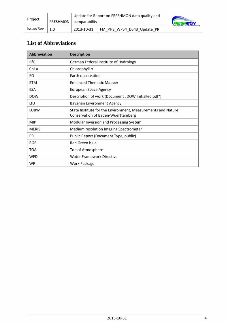
List of Abbreviations
Abbreviation Description
BfG German Federal Institute of Hydrology
Chl-a Chlorophyll a
EO Earth observation
ETM Enhanced Thematic Mapper
ESA European Space Agency
DOW Description of work (Document „DOW Initialled.pdf“)
LfU Bavarian Environment Agency
LUBW State Institute for the Environment, Measurements and Nature Conservation of Baden-Wuerttemberg
MIP Modular Inversion and Processing System
MERIS Medium resolution Imaging Spectrometer
PR Public Report (Document Type, public)
RGB Red Green blue
TOA Top of Atmosphere
WFD Water Framework Directive
WP Work Package

Project FRESHMON
Update for Report on FRESHMON data quality and
comparability
Issue/Rev 1.0 2013-10-31 FM_PH3_WP54_D543_Update_PR
2013-10-31 5
1 Scope of this document
This document is an update to D54.3 “Report on FRESHMON data quality and data comparability”.
The original D54.3 described the results of the validation activities performed in FRESHMON until
October 2012. This document describes the validation done between November 2012 and October
2013. It includes results for three satellite instruments (MERIS, Landsat ETM+, and WorldView-2). The
in situ data used in the validation includes measurements done by FRESHMON partners and data
provided by user organizations.
Related FRESHMON-documents:
- D54.1 Radiometric and in situ measurements of the ground truth for assessing the services
(delivered 11/2011) describes the measurements made during the 1st phase of the project.
- D54.2 Radiometric and in situ measurements of the ground truth for assessing the services
(delivered 10/2012) describes the measurements made during the 2nd phase of the project.
- D54.3 Report on FRESHMON data quality and data comparability (delivered 10/2012)
describes the results of the validation effort until October 2012.
- D52.1 Report on Case Studies for practicability (delivered 10/2012) will describe in detail the
in situ measurements made by EAWAG for the Lake Constance Field Campaign.
2 Executive Summary
Satellite products from FRESHMON phase 3 have been validated with in situ data in Finland (MERIS
Chl-a and WorldView-2 water depth) and Germany (MERIS Chl-a, and MERIS and Landsat 7 ETM+
turbidity and suspended matter).
In situ data suitable for EO validation is still lacking in many places since the collection of field
samples has not been optimized for EO purposes. Due to this, it is convenient to present the results
for Chl-a and turbidity/TSM as time series plots since with those the behavior of EO estimates and in
situ measurements can be compared from season to season and year to year. The time series plots
make it is possible to analyze where the EO methods work well and where more research (or another
instrument) is needed. Problematic areas are small lakes where the resolution of MERIS is not
sufficient and in Finland the humic lakes where the absorption by CDOM affects the retrieval of Chl-a.
The water depth estimation works well down to a depth of 2 to 3 m. Turbidity in water and
atmospheric effects can limit the usability of images.
As result of the validation, the EO based products – both MERIS based data with a high temporal
resolution and Landsat based with high spatial resolution – generate very valuable additional
information for monitoring aspects and scientific questions.
Lessons learnt in the FRESHMON product validation include taking care about time coincidence,
location dependence and measurement depth information. Further improvements can be made
using pixel wise quality control and data aggregation in the validation process.

Project FRESHMON
Update for Report on FRESHMON data quality and
comparability
Issue/Rev 1.0 2013-10-31 FM_PH3_WP54_D543_Update_PR
2013-10-31 6
3 Validation in Finland (SYKE)
In Finland the validation of satellite products took place in the areas shown in Figure 1. In the area
Southern Finland, MERIS Chl-a products were compared with in situ observations. In Hanko and
Kotka areas water depth products derived from WorldView-2 data were tested.
Figure 1. Satellite data validation areas in Finland (indicated with red).
Southern Finland
Hanko
Kotka
Project FRESHMON
Update for Report on FRESHMON data quality and
comparability
Issue/Rev 1.0 2013-10-31 FM_PH3_WP54_D543_Update_PR
2013-10-31 7
3.1 MERIS Chl-a
Finland has over 56 000 lakes (size > 1 ha) and the number of lake water bodies defined by the Water
Framework Directive (WFD) is almost 4300. About 60% of them were not ecologically classified in the
last WFD reporting due to lack of monitoring data. E.g. Chlorophyll a (Chl-a), a measure algal biomass
and indicates lake’s trophic status, is annually measured only in about 1400 lakes.
Hence, in Finland, the main objective for the 3rd phase of FRESHMON was to provide data for inland
water body classification performed under the WFD. We took advantage of the work done for coastal
areas, where product types suitable for WFD monitoring had already been drafted. In addition to
providing water quality (Chl-a, turbidity, SST) maps from the Baltic Sea, SYKE has provided EO and in
situ time series plots and histograms of Chl-a for 188 (out of 214) coastal monitoring areas.
This chapter describes the steps taken to process the satellite and in situ data, and shows examples
of the results for lakes.
3.1.1 MERIS data processing
During the second phase of FRESHMON, MERIS Chl-a products were processed with BEAM and then
calibrated with raft data (see D54.3 for details). The results show that there is a good correlation
between satellite observations and the values measured by an in situ fluorometer. In D54.3 the
equation used to calibrate satellite data was:
Chl-aCalib = 0.346* Chl-aSatellite + 3.76, (1) where Chl-aSatellite is the original estimate from the processing chain. While the calibration leads to
good results with the lake where the raft is, it causes some problems when the method is used for
other water bodies. First of all, the bias term of 3.76 g/l sets the lower limit of the estimation range.
This is too high since there are lakes in Finland that have Chl-a concentrations of about 1 g/l and for
some lake types the classification limit between classes High and Good is 2 g/l (for lakes in northern
Lapland), 3 g/l (for humus-poor lakes) or 3.3 g/l (for Shallow humus-poor lakes). So, with Equation
(1), Chl-a concentrations belonging to the High class would never be obtained in these lake types.
The higher end of the estimation range of the FUB processor is 120 g/l for Chl-a so the slope term of
0.346 (and the bias) set the maximum calibrated value to about 45 g/l. This in turn is too low for
many eutrophic lakes where the concentration measured with in situ laboratory samples have been
over 100 g/l.
Due to this the processing steps of MERIS data were revised for the inland WFD water bodies and are
the following (with BEAM 4.10.3):
1. AMORGOSS for improved geolocation
2. Radiometry correction (Smile, & Equalization, as the MERIS data was from the 3rd
reprocessing the Calibration step was not included)
3. FUB/WeW 1.2.8 (water quality processing)
4. Rectification
5. Land and cloud masking (see below)
6. Product generation

Project FRESHMON
Update for Report on FRESHMON data quality and
comparability
Issue/Rev 1.0 2013-10-31 FM_PH3_WP54_D543_Update_PR
2013-10-31 8
The new processing does not include empirical correction. The products were stored as GeoTiff files,
which were used in the further processing and published through a WMS.
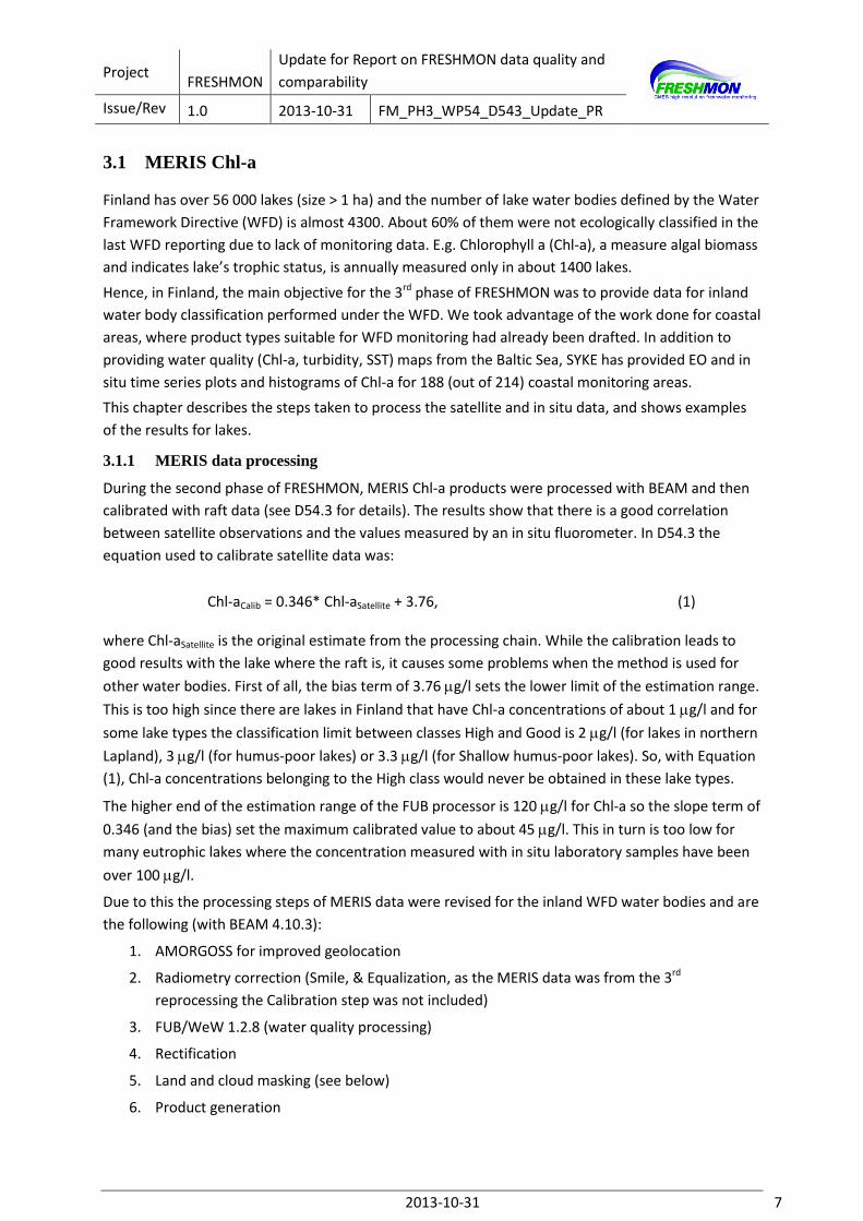
So far the summer months (June-Sep) of years 2006, 2009 and 2011 have been processed from
Southern Finland. Figure 2 shows an example Chl-a map. Figure 3 shows the effect of AMORGOS on
the products. When AMORGOS is not included in the processing there are more red (non-valid high-
concentration) pixels near the shore. Hence, the results are better with AMORGOS included in the
processing.
MERIS data used in this analysis were provided by ESA.
Figure 2. MERIS Chl-a map of Southern Finland on June 16, 2006.
Project FRESHMON
Update for Report on FRESHMON data quality and
comparability
Issue/Rev 1.0 2013-10-31 FM_PH3_WP54_D543_Update_PR
2013-10-31 9
Without AMORGOS With AMORGOS
Figure 3. The effect of AMORGOS on the Chl-a products. The number of erroneous red (high concentration) pixels is reduced when AMORGOS is used in the processing.
3.1.2 Land and cloud masks
Land (and Baltic Sea) areas are masked from the product images using a mask derived from shore
line data. The mask is made with a regular grid (300 m pixels) which is also used in the rectification
step and is the same for all products. If a pixel contains even a small amount of land according to the
shore line data, it is classified as land.
The cloud mask is derived from the processed data. All pixels with Chl-a value of 100 000 (as
generated by FUB) are classified as clouds. This initial cloud mask is then buffered by 4 pixels in each
direction in order to reduce the errors caused by cloud shadows and thin clouds that often surround
thick clouds and are difficult to detect.
3.1.3 In situ data
The in situ data used in this analysis come from the routine monitoring programme implemented in
Finland. Under the programme, water samples are collected by regional environmental authorities
and companies (who often outsource the sample collection and analysis to consulting companies)
required to monitor water bodies as part of their environmental license to operate e.g. a factory. Chl-
a concentrations, representing a 0-2 m surface layer, were analyzed from the samples in a laboratory
with spectrophotometric determination after extraction with hot ethanol (ISO 10260, GF/C filter).

Project FRESHMON
Update for Report on FRESHMON data quality and
comparability
Issue/Rev 1.0 2013-10-31 FM_PH3_WP54_D543_Update_PR
2013-10-31 10
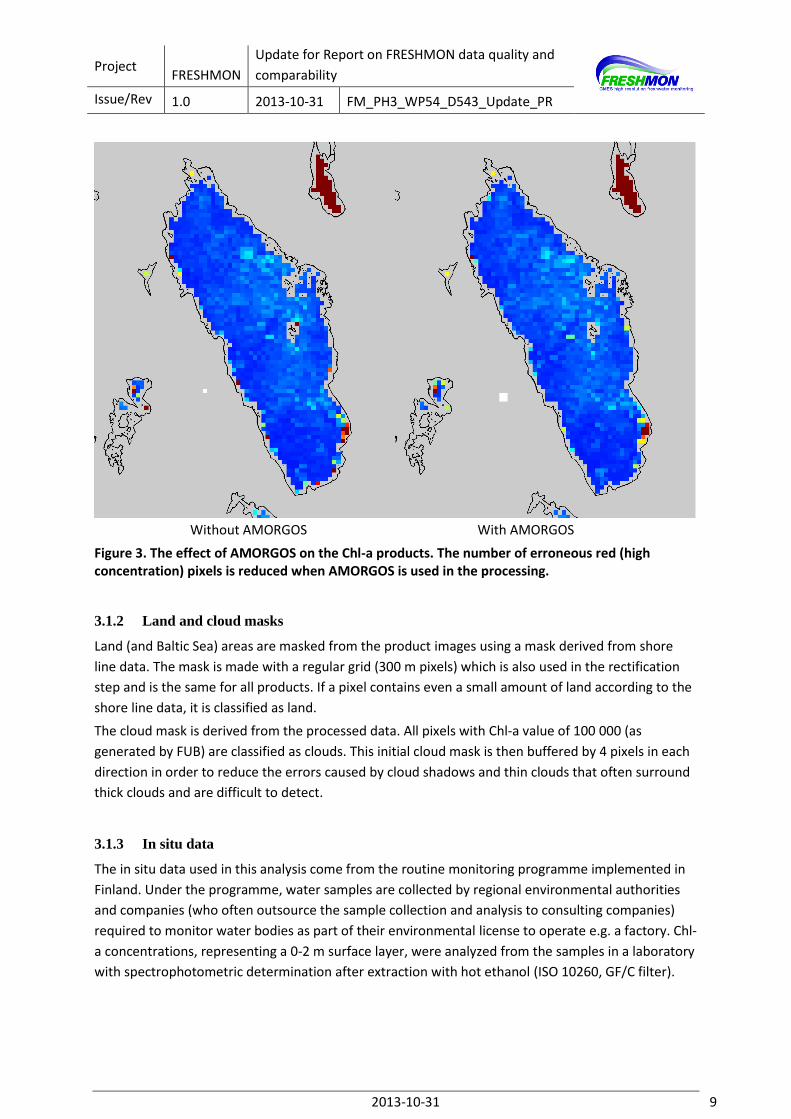
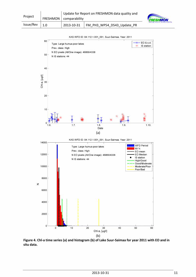
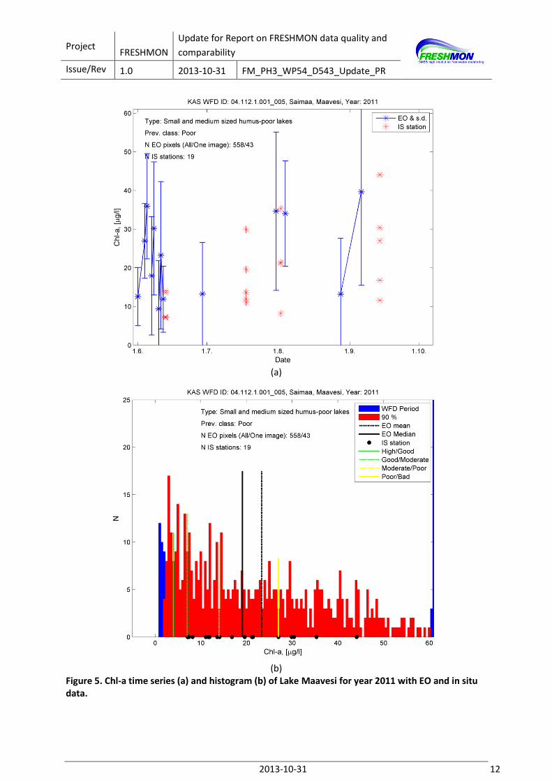
3.1.4 Data aggregation and visualization
The monitoring areas of WFD are defined as vectors in shape files. These were used to extract the
pixel values found within each monitoring area and from each GeoTiff image.
The mean and standard deviation of the pixel values were computed and once the whole year was
processed time series and histogram plots were generated for each monitoring area in Southern
Finland. Example results are shown in Figure 4 and Figure 5.
The number of WFD water bodies within the study area (Figure 1) is 2271. Due to the limited
resolution of MERIS (300 m) small lakes cannot be monitored with it. For this processing, we set a
size limit so that the water body must contain at least 3 MERIS pixels before it is included in the
analysis. After this restriction the number of water bodies was 662. For all these the time series and
histogram plots were generated. It should be noted the number of lakes might vary slightly, if the
coordinate grid of reference for defining the rectified MERIS data was shifted with distance less than
half of the nominal resolution, or if different coordinate systems were used in rectification. As the
number of small lakes is high, and they are effectively randomly located, this does not have
significant impact on the results.
In addition, if the number of cloud free pixels extracted from the water body was less than 90% of
the maximum number of pixels for that water body (based on the landmask) the values from that
day were included in the result plots. This will further reduce the effects of cloud cover on the time
series analysis.
When this analysis was performed the number WFD of water bodies defined for the whole Finland
was 4276. Figure 6 shows how many of these can be monitored with a 300 m pixel instrument (e.g.
MERIS and Sentinel-3 OLCI) as a function of the minimum number of pixels that fit into the water
bodies. At least one 300 m pixel can be found from over 2100 water bodies, however, one pixel is
rarely enough for a reliable estimate of water quality. If the minimum number of pixels per water
body is set to 10 the number of possible water bodies is less than 700. Furthermore, this
computation is theoretical in nature and includes shallow and other areas that may be impossible to
monitor with EO. This will slightly reduce the number of water bodies suitable for EO monitoring.
Project FRESHMON
Update for Report on FRESHMON data quality and
comparability
Issue/Rev 1.0 2013-10-31 FM_PH3_WP54_D543_Update_PR
2013-10-31 11
(a)
(b)
Figure 4. Chl-a time series (a) and histogram (b) of Lake Suur-Saimaa for year 2011 with EO and in situ data.
Project FRESHMON
Update for Report on FRESHMON data quality and
comparability
Issue/Rev 1.0 2013-10-31 FM_PH3_WP54_D543_Update_PR
2013-10-31 12
(a)
(b)
Figure 5. Chl-a time series (a) and histogram (b) of Lake Maavesi for year 2011 with EO and in situ data.

Project FRESHMON
Update for Report on FRESHMON data quality and
comparability
Issue/Rev 1.0 2013-10-31 FM_PH3_WP54_D543_Update_PR
2013-10-31 13
0 10 20 30 40 50 60 70 80 90 100 1100
200
400
600
800
1000
1200
1400
1600
1800
2000
2200
Minimum number of MERIS pixels in the water body
Nu
mb
er
of w
ate
r b
od
ies
2102
391
1296
303
695
201266
83172
54
3
Normal landmask
Buffered landmask
Figure 6. The number of Finnish lake WFD water bodies as a function of the minimum number of MERIS pixels that fit inside the water body with two land masks. In the buffered land mask, the mask is extended by one extra pixel from the shore.
3.1.5 Effects of CDOM on Chl-a estimation
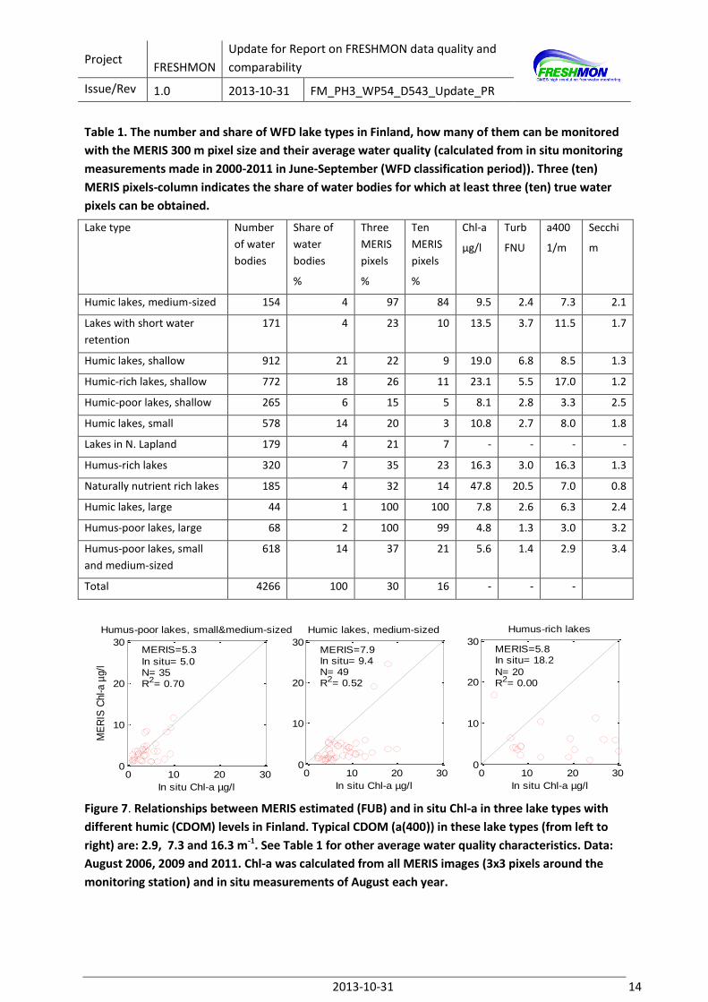
Finnish lakes are in WFD divided into 12 lake types, the main criteria being humic level, size and
depth (Table 1). The share of those water bodies that can be monitored with MERIS varies
considerably by lake type.
The impact of humic concentration in the estimation of Chl-a by FUB is demonstrated in Figure 7. In
humic-poor lakes FUB is able to estimate Chl-a quite realistically, while in humic-rich lakes FUB
systematically underestimates Chl-a and there is no correlation. In humic lakes, with CDOM (a400)
typically between 3.3 and 11 m-1, the FUB underestimates Chl-a, but there is linear correlation with
the in situ Chl-a. This indicates that Chl-a can be estimated with FUB in humic lakes, but estimates
must be empirically corrected or the processor must be modified in order to get correct absolute
concentrations.
There are two high-CDOM lake types (with a400>11 m-1) in the Finnish typology: humic-rich lakes and
shallow humic-rich lakes (Table 1). These lake types represent 7 and 18% of all water bodies,
respectively. The impact of high CDOM on remote sensing based estimation of Chl-a also depends on
the concentration of particles in water. The limitations must be further studied particularly in the
shallow humic lakes where water quality varies more than in the deep lakes.
Project FRESHMON
Update for Report on FRESHMON data quality and
comparability
Issue/Rev 1.0 2013-10-31 FM_PH3_WP54_D543_Update_PR
2013-10-31 14
Table 1. The number and share of WFD lake types in Finland, how many of them can be monitored
with the MERIS 300 m pixel size and their average water quality (calculated from in situ monitoring
measurements made in 2000-2011 in June-September (WFD classification period)). Three (ten)
MERIS pixels-column indicates the share of water bodies for which at least three (ten) true water
pixels can be obtained.
Lake type Number
of water
bodies
Share of
water
bodies
%
Three
MERIS
pixels
%
Ten
MERIS
pixels
%
Chl-a
µg/l
Turb
FNU
a400
1/m
Secchi
m
Humic lakes, medium-sized 154 4 97 84 9.5 2.4 7.3 2.1
Lakes with short water
retention
171 4 23 10 13.5 3.7 11.5 1.7
Humic lakes, shallow 912 21 22 9 19.0 6.8 8.5 1.3
Humic-rich lakes, shallow 772 18 26 11 23.1 5.5 17.0 1.2
Humic-poor lakes, shallow 265 6 15 5 8.1 2.8 3.3 2.5
Humic lakes, small 578 14 20 3 10.8 2.7 8.0 1.8
Lakes in N. Lapland 179 4 21 7 - - - -
Humus-rich lakes 320 7 35 23 16.3 3.0 16.3 1.3
Naturally nutrient rich lakes 185 4 32 14 47.8 20.5 7.0 0.8
Humic lakes, large 44 1 100 100 7.8 2.6 6.3 2.4
Humus-poor lakes, large 68 2 100 99 4.8 1.3 3.0 3.2
Humus-poor lakes, small
and medium-sized
618 14 37 21 5.6 1.4 2.9 3.4
Total 4266 100 30 16 - - -
Figure 7. Relationships between MERIS estimated (FUB) and in situ Chl-a in three lake types with
different humic (CDOM) levels in Finland. Typical CDOM (a(400)) in these lake types (from left to
right) are: 2.9, 7.3 and 16.3 m-1. See Table 1 for other average water quality characteristics. Data:
August 2006, 2009 and 2011. Chl-a was calculated from all MERIS images (3x3 pixels around the
monitoring station) and in situ measurements of August each year.
0 10 20 300
10
20
30
In situ Chl-a µg/l
ME
RIS
Chl-a µ
g/l
Humus-rich lakes
MERIS=5.8In situ= 18.2
N= 20R2= 0.00
0 10 20 300
10
20
30
In situ Chl-a µg/l
ME
RIS
Chl-a µ
g/l
Humic lakes, medium-sized
MERIS=7.9In situ= 9.4N= 49R2= 0.52
0 10 20 300
10
20
30
In situ Chl-a µg/l
ME
RIS
Chl-a µ
g/l
Humus-poor lakes, small&medium-sized
MERIS=5.3
In situ= 5.0N= 35R2= 0.70
Project FRESHMON
Update for Report on FRESHMON data quality and
comparability
Issue/Rev 1.0 2013-10-31 FM_PH3_WP54_D543_Update_PR
2013-10-31 15
Figure 8 shows the in situ remote sensing reflectance spectra (Rrs) measured from five lakes in
Finland with a portable spectrometer (ASD Pro Jr.), while Table 2 shows the corresponding results of
the lab measurements. In lakes Säkylän Pyhäjärvi and Vesijärvi the CDOM absorption is low and
reflectance values high. In lakes Lammin Pääjärvi and Keravanjärvi the situation is the opposite.
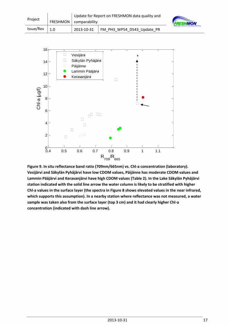
One important feature of the spectra is the peak near 700 nm and the dip near 670 nm. The size of
the peak in relation to the dip has been observed to grow with increasing Chl-a concentrations and
several Chl-a estimation algorithms that take advantage of this have been developed (starting with
Dekker (1993) and Gitelson et al. (1993)). Figure 9 shows a comparison of a reflectance band ratio vs.
Chl-a concentration for the five lakes. While the number of data points is small and the results are
preliminary, the correlation between the band ratio and Chl-a concentration appears to be high if the
data points are grouped according to CDOM class. Same behavior has been noted with reflectance
data simulated with a large in situ concentration dataset measured from Finnish lakes (Kallio 2006).
This also indicates that the Chl-a estimation can be improved, if information about the CDOM
absorption is available.
The situation becomes more complex when algorithms based on neural networks trained with
simulated data (such as the FUB processor) are used in the estimation. They contain nodes which
convert the input values (reflectances and other parameters) into output values (water quality
parameters) using weights defined during the training. Once the network has been trained it is not
possible to modify it and if the measured water type is not included in the training data the results
can be unreliable.
In addition, atmospheric correction, which is the most critical part of the water quality processing, is
typically also based on neural networks. Strong CDOM absorption is usually not included in the
models and the FUB processor regularly processes negative reflectances for humic lakes.
3.1.6 User comments
Based on the user comments in D54.3 several topics for further research were identified. These are
shown in Table 3 together with the current status of the research. Table 4 in turn shows the user
comments for the data provided in Phase 3 and the response of FRESHMON to these comments.

Project FRESHMON
Update for Report on FRESHMON data quality and
comparability
Issue/Rev 1.0 2013-10-31 FM_PH3_WP54_D543_Update_PR
2013-10-31 16
Figure 8. In situ remote sensing reflectance spectra from Finland measured with ASD spectrometer.
Table 2. In situ measurements from Finland in 2007, 2011 and 2013.
Lake and station number
Date (YYYYMMDD) Local time
Secchi depth (m)
Chl a (ug/l)
Turbidity (FNU)
aCDOM(400) (1/m)
TSM (mg/l)
Vesijärvi 1 20070604 11:20 2,9 3,7 3 1,76 2,6
Vesijärvi 2 20070604 13:10 3,7 2,9 2,3 1,38 2
Vesijärvi 3 20070807 11:10 2,9 4,6 1,9 1,1 2,2
Vesijärvi 4 20070807 12:20 4,6 1,7 1,1 0,9 1,2
Vesijärvi 5 20110609 11:15 2,8 5,4 2,4 1,57 3,4
Vesijärvi 6 20110609 12:30 3,1 5,1 2,3 1,52 3
Vesijärvi 7 20130905 11:30 2,4 11 3,6 1,80 2,5
Päijänne 1 20070604 1130 5 2,1 0,86 2,82 0,8
Päijänne 2 20070807 10:53 4,9 1,9 0,62 2,5 0,7
Säkylän Pyhäjärvi 1 20070823 11:05 3,5 5,3 1,7 1,6 2
Säkylän Pyhäjärvi 2 20070823 11:40 3,6 5,4 1,5 1,5 2
Säkylän Pyhäjärvi 3 20070823 12:15 3,6 7,2 2,3 1,5 2
Lammin Pääjärvi 1 20110629 10:10 2,3 3,2 1,3 9,63 1,9
Lammin Pääjärvi 2 20130618 09:45 2,2 3 1,7 12,10 1,2
Lammin Pääjärvi 3 20130823 10:40 2,1 1,59 0,76 11,23 0,9
Keravanjärvi 1 20130806 11:05 1,3 8,2 2,1 20,43 2,1
Project FRESHMON
Update for Report on FRESHMON data quality and
comparability
Issue/Rev 1.0 2013-10-31 FM_PH3_WP54_D543_Update_PR
2013-10-31 17
0.4 0.5 0.6 0.7 0.8 0.9 1 1.10
2
4
6
8
10
12
14
16
R709
/R665
Ch
l-a
( g
/l)
Vesijärvi
Säkylän Pyhäjärvi
Päijänne
Lammin Pääjärvi
Keravanjärvi
Figure 9. In situ reflectance band ratio (709nm/665nm) vs. Chl-a concentration (laboratory).
Vesijärvi and Säkylän Pyhäjärvi have low CDOM values, Päijänne has moderate CDOM values and
Lammin Pääjärvi and Keravanjärvi have high CDOM values (Table 2). In the Lake Säkylän Pyhäjärvi
station indicated with the solid line arrow the water column is likely to be stratified with higher
Chl-a values in the surface layer (the spectra in Figure 8 shows elevated values in the near infrared,
which supports this assumption). In a nearby station where reflectance was not measured, a water
sample was taken also from the surface layer (top 3 cm) and it had clearly higher Chl-a
concentration (indicated with dash line arrow).
Project FRESHMON
Update for Report on FRESHMON data quality and
comparability
Issue/Rev 1.0 2013-10-31 FM_PH3_WP54_D543_Update_PR
2013-10-31 18
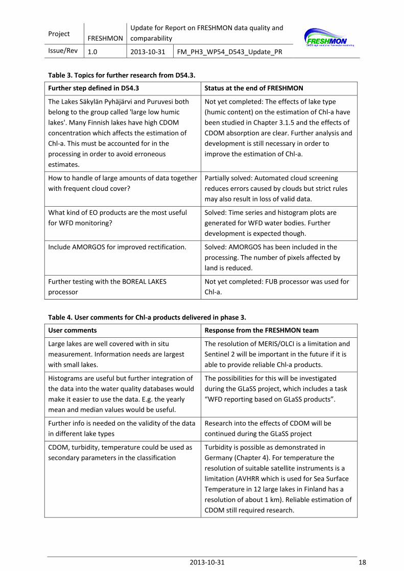
Table 3. Topics for further research from D54.3.
Further step defined in D54.3 Status at the end of FRESHMON
The Lakes Säkylän Pyhäjärvi and Puruvesi both
belong to the group called 'large low humic
lakes'. Many Finnish lakes have high CDOM
concentration which affects the estimation of
Chl-a. This must be accounted for in the
processing in order to avoid erroneous
estimates.
Not yet completed: The effects of lake type
(humic content) on the estimation of Chl-a have
been studied in Chapter 3.1.5 and the effects of
CDOM absorption are clear. Further analysis and
development is still necessary in order to
improve the estimation of Chl-a.
How to handle of large amounts of data together
with frequent cloud cover?
Partially solved: Automated cloud screening
reduces errors caused by clouds but strict rules
may also result in loss of valid data.
What kind of EO products are the most useful
for WFD monitoring?
Solved: Time series and histogram plots are
generated for WFD water bodies. Further
development is expected though.
Include AMORGOS for improved rectification. Solved: AMORGOS has been included in the
processing. The number of pixels affected by
land is reduced.
Further testing with the BOREAL LAKES
processor
Not yet completed: FUB processor was used for
Chl-a.
Table 4. User comments for Chl-a products delivered in phase 3.
User comments Response from the FRESHMON team
Large lakes are well covered with in situ
measurement. Information needs are largest
with small lakes.
The resolution of MERIS/OLCI is a limitation and
Sentinel 2 will be important in the future if it is
able to provide reliable Chl-a products.
Histograms are useful but further integration of
the data into the water quality databases would
make it easier to use the data. E.g. the yearly
mean and median values would be useful.
The possibilities for this will be investigated
during the GLaSS project, which includes a task
“WFD reporting based on GLaSS products”.
Further info is needed on the validity of the data
in different lake types
Research into the effects of CDOM will be
continued during the GLaSS project
CDOM, turbidity, temperature could be used as
secondary parameters in the classification
Turbidity is possible as demonstrated in
Germany (Chapter 4). For temperature the
resolution of suitable satellite instruments is a
limitation (AVHRR which is used for Sea Surface
Temperature in 12 large lakes in Finland has a
resolution of about 1 km). Reliable estimation of
CDOM still required research.
Project FRESHMON
Update for Report on FRESHMON data quality and
comparability
Issue/Rev 1.0 2013-10-31 FM_PH3_WP54_D543_Update_PR
2013-10-31 19
3.2 High resolution water depth products near Hanko and Kotka
The objective of this chapter was to find out how well satellite based (WorldView-2) water depth
maps match with in situ observations.
3.2.1 Study area and satellite data
Two different test sites were selected for this study. One site is located near Hanko, in the Western
Gulf of Finland where the bottom is sandy and sandbanks are common. Another test site located at
the Easter part of Gulf of Finland characterized by steep rock shores and esker islands. Field data of
water depth was collected in VELMU-program (Finnish Marine Underwater Nature Inventory
Programme) during sampling seasons 2008-2012 and values were corrected with sea level measured
by the Finnish Meteorological Institute.
The WorldView-2 images used in the analysis were taken on 29.4.2011 (Hanko) and 4.9.2012 (Kotka).
WorldView-2 is multispectral satellite sensor with eight optical bands and 2m spatial resolution.
Compared to other very high resolution satellites it has three new interesting bands: violet (coastal),
yellow and red edge. Satellite images were georectified by using shoreline-layer.
3.2.2 Satellite data processing
EOMAP generated water depth product for 29.4.2011 (Hanko) and 4.9.2012 (Kotka) and images with
the MIP processor, comprising a coupled retrieval of atmospheric and in-water optical properties
(Ohlendorf et al. 2011). As the result of atmospheric correction, the subsurface reflectance is
retrieved.
The transformation of the subsurface reflectance to bottom reflectance is based on the equations
published by Albert and Mobley (2003). The water depth, which is originally an input value for these
equations, is iteratively calculated in combination with the spectral unmixing of the corresponding
bottom reflectance. By minimizing the residual error the final water depth is determined. This
processing step results in two output images, one image containing water depth and another image
containing bottom reflectances.
The production of water depth products was tested also at SYKE (by the Marine Research Centre) for
the two images. Based on the idea that light is attenuating exponentially when the depth is
increasing, Lyzenga (1978) showed the equation between the remote sensing reflectance and the
water depth. Lyzenga’s model shows that light will penetrate water depending on its wavelength and
this information can be used to determine depth from satellite images. The model however assumes
that water quality is homogeneous throughout the image and it requires information about the
reflection properties of different bottom types. Stumpf et al. (2003) proposed “a ratio method”
which reduces the effect of bottom substrate. The method is based on the Lyzenga’s algorithm but it
utilizes two bands to derive the depth. By using this method the change in attenuation of different
colored light is much greater than the change affected by bottom reflectance in different bands. This
method can then be used to derive depth over varying bottom substrates.
At SYKE the Stumpf et al. (2003) model was applied to both satellite images. Changes in water quality
were taken into account by dividing satellite images into several smaller processing areas based on
their turbidity. The best band combinations were tested and some local changes in the equation
were done with a set of field measurements (N=249 in Hanko and N=88 in Kotka). Half of the field
measurements were used for calibration and half for validation (see below).

Project FRESHMON
Update for Report on FRESHMON data quality and
comparability
Issue/Rev 1.0 2013-10-31 FM_PH3_WP54_D543_Update_PR
2013-10-31 20
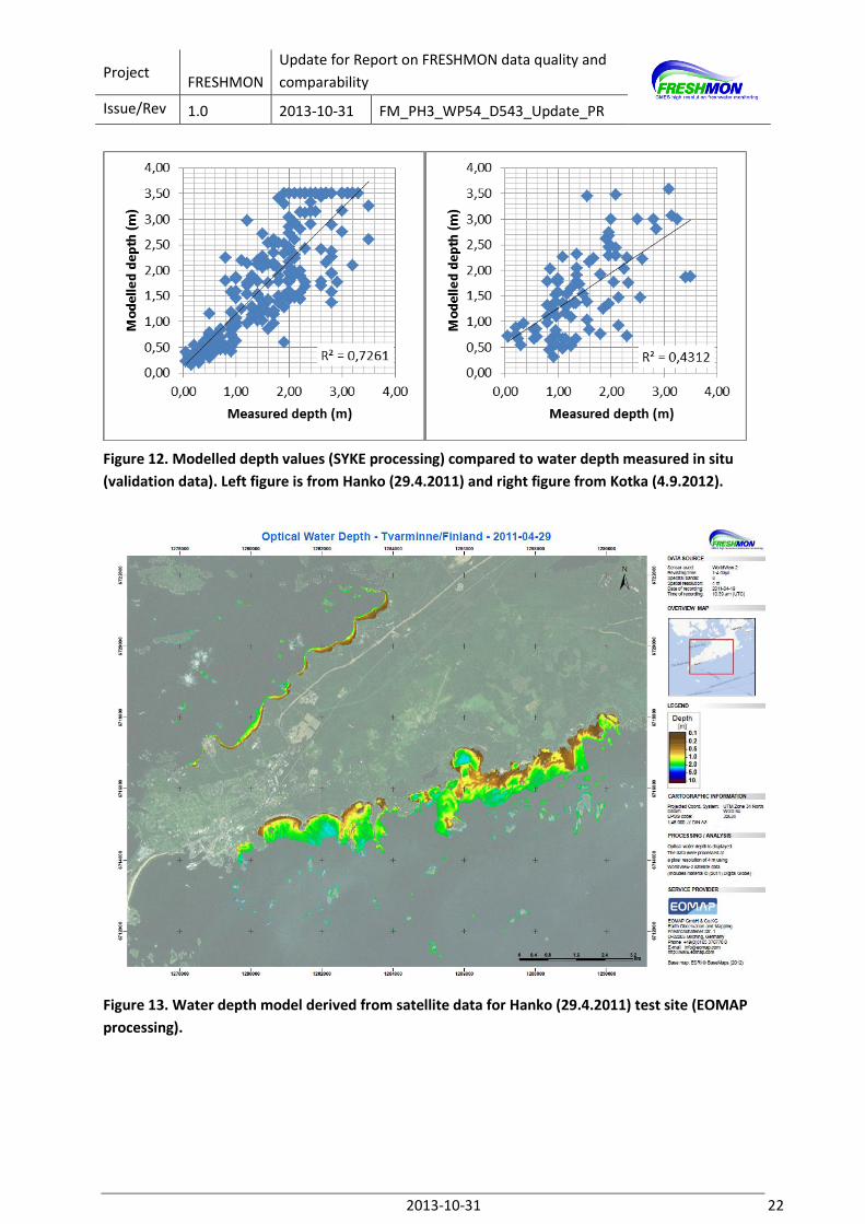
3.2.3 Results
The results of the model used by SYKE are shown in Figure 10 (Hanko) and Figure 11 (Kotka). The
accuracy of the model was tested by comparing the estimated values with field samples (Figure 12).
In Hanko the SYKE model was shown to be quite accurate at least in shallow areas but the error was
increasing with the depth. In Kotka the model was less accurate than in Hanko due to turbid water
and unclear atmosphere. The shallowest areas have too high depth values which may be due the
steep shores and the reflection from the land areas. The model is still capable of finding ecologically
important shallow areas and gives accurate estimates of water depth in those areas.
The result of the processing done at EOMAP is shown in Figure 13 for the 29.4.2011 (Hanko) image.
The results of the comparison of EO values vs. in situ values are shown in Figure 14 (with all available
stations). Due to high turbidity in water, the processing was successful only for a small portion of the
4.9.2012 (Kotka) image and the results did not cover the study area well. Thus, a comparison with in
situ data was not possible. Instead, the results by EOMAP were compared with the results from SYKE
(Figure 15).
According to the results, the EOMAP processing works well for shallow water areas (<2 m). As
evident in the plots, the EO values are slightly underestimated but this can be corrected by
calibrating the result with in situ observations when those are available. Since water depth does not
change quickly, the in situ measurements do not have to be concurrent with the satellite overpass if
information about the sea level is available (i.e. data from different years can be used). For deeper
water the estimation errors are larger. Fortunately, the users were more interested in shallow water
areas. The cut-off depth (the largest estimated depth) appears to be about 2.5 to 3.5 m depending
on the processing and the area (differences in water quality).

Project FRESHMON
Update for Report on FRESHMON data quality and
comparability
Issue/Rev 1.0 2013-10-31 FM_PH3_WP54_D543_Update_PR
2013-10-31 21
Figure 10. Water depth model derived from satellite data for Hanko (29.4.2011) test site (SYKE
processing).
Figure 11. Water depth model derived from satellite data for a small part of Kotka (4.9.2012) test
site (SYKE processing).
Project FRESHMON
Update for Report on FRESHMON data quality and
comparability
Issue/Rev 1.0 2013-10-31 FM_PH3_WP54_D543_Update_PR
2013-10-31 22
Figure 12. Modelled depth values (SYKE processing) compared to water depth measured in situ
(validation data). Left figure is from Hanko (29.4.2011) and right figure from Kotka (4.9.2012).
Figure 13. Water depth model derived from satellite data for Hanko (29.4.2011) test site (EOMAP
processing).

Project FRESHMON
Update for Report on FRESHMON data quality and
comparability
Issue/Rev 1.0 2013-10-31 FM_PH3_WP54_D543_Update_PR
2013-10-31 23
Figure 14. Modeled depth values compared to water depth measured in situ from Hanko
(29.4.2011) with EOMAP processing (validation data).
Figure 15. Water depth values estimated from satellite data by EOMAP compared to water depth
values estimated from satellite data by SYKE from the Kotka (4.9.2012) image.
Project FRESHMON
Update for Report on FRESHMON data quality and
comparability
Issue/Rev 1.0 2013-10-31 FM_PH3_WP54_D543_Update_PR
2013-10-31 24
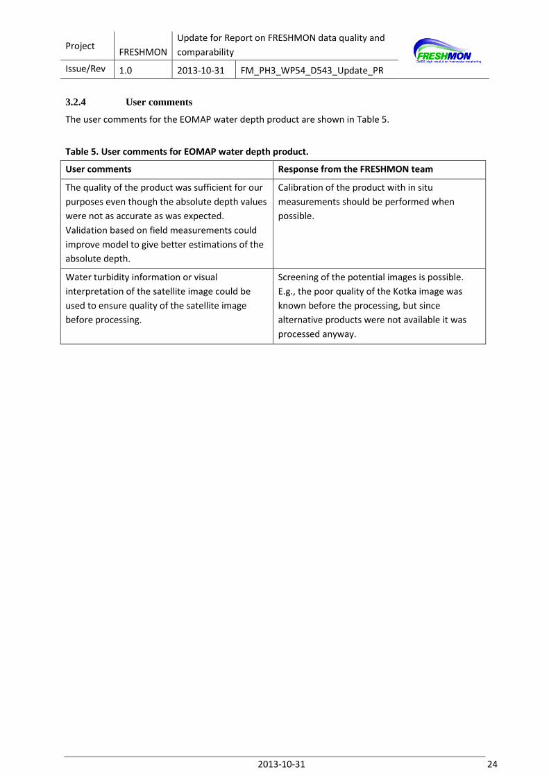
3.2.4 User comments
The user comments for the EOMAP water depth product are shown in Table 5.
Table 5. User comments for EOMAP water depth product.
User comments Response from the FRESHMON team
The quality of the product was sufficient for our
purposes even though the absolute depth values
were not as accurate as was expected.
Validation based on field measurements could
improve model to give better estimations of the
absolute depth.
Calibration of the product with in situ
measurements should be performed when
possible.
Water turbidity information or visual
interpretation of the satellite image could be
used to ensure quality of the satellite image
before processing.
Screening of the potential images is possible.
E.g., the poor quality of the Kotka image was
known before the processing, but since
alternative products were not available it was
processed anyway.

Project FRESHMON
Update for Report on FRESHMON data quality and
comparability
Issue/Rev 1.0 2013-10-31 FM_PH3_WP54_D543_Update_PR
2013-10-31 25
4 Validation in Germany (EOMAP and BC)
4.1 Lakes in South Germany-MERIS vs. Landsat
4.1.1 Satellite data validation
In continuation of the validation conducted for the MERIS data in various lakes in South Germany in
the FRESHMON deliverable D54.3, we compared the results of the Landsat 7 ETM+ processing
products with the results of a set of selected lakes (Lake Constance station FU, Ammersee and
Walchensee, see Figure 16).
For the validation, we selected the available Landsat 7 ETM+ imagery with suitable cloud coverage
for the years 2004-2012.
Figure 16. Lake Constance station FU, Ammersee and Walchensee
Project FRESHMON
Update for Report on FRESHMON data quality and
comparability
Issue/Rev 1.0 2013-10-31 FM_PH3_WP54_D543_Update_PR
2013-10-31 26
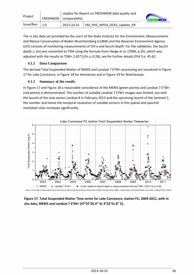
The in situ data set provided by the users of the State Institute for the Environment, Measurements
and Nature Conservation of Baden-Wuerttemberg (LUBW) and the Bavarian Environment Agency
(LfU) consists of monitoring measurements of Chl-a and Secchi depth. For the validation, the Secchi
depth zs [m] was converted to TSM using the formula from Heege et al. (1998, p.25), which was
adjusted with the results to TSM= 2.65*(1/ln zs-0.28), see for further details D54.3 p. 45-62.
4.1.2 Data Comparison
The derived Total Suspended Matter of MERIS and Landsat 7 ETM+ processing are visualized in Figure
17 for Lake Constance, in Figure 18 for Ammersee and in Figure 19 for Walchensee.
4.1.3 Summary of the results
In Figure 17 and Figure 18 a reasonable coincidence of the MERIS (green points) and Landsat 7 ETM+
(red points) is demonstrated. The number of suitable Landsat 7 ETM+ images was limited, but with
the launch of the new sensor Landsat 8 in February 2013 and the upcoming launch of the Sentinel 2,
the number and hence the temporal resolution of suitable sensors in this spatial and spectral
resolution class increases significantly.
Figure 17. Total Suspended Matter Time series for Lake Constance, station FU, 2004-2011, with in
situ data, MERIS and Landsat 7 ETM+ (47°37’26.4’’ N, 9°22’31.8’’ E).

Project FRESHMON
Update for Report on FRESHMON data quality and
comparability
Issue/Rev 1.0 2013-10-31 FM_PH3_WP54_D543_Update_PR
2013-10-31 27
Figure 18. Total Suspended Matter Time series for Lake Ammersee, 2004-2011, with in situ data,
MERIS and Landsat 7 ETM+ (47°58’55.71’’ N, 11°7’20.62’’ E).
Figure 19. Total Suspended Matter Time series for Walchensee 2003-2011, with in situ data, MERIS
and Landsat 7 ETM+ (47°36’5.74’’ N, 11°20’46.66’’ E).
Project FRESHMON
Update for Report on FRESHMON data quality and
comparability
Issue/Rev 1.0 2013-10-31 FM_PH3_WP54_D543_Update_PR
2013-10-31 28
4.2 Bavarian Rivers
For the validation of the satellite based turbidity product in Bavarian Rivers, we analyzed the in situ
data of suspended matter provided by the Bavarian Environment Agency LfU (production series
S_cMess) in mg/m³ in comparison to the turbidity product derived from the MIP (EOMAP) processing
of Landsat 7 ETM+ data, see Table 6 for the overview of the data set.
The in situ data until end of 2008 are considered as tested/checked values, after this date the data
have to be considered as raw data (comment by LfU). To collect a reasonable data set with
coincident dates, we chose the stations Füssen for river Lech, Passau Ingling for river Inn and
München for river Isar, see Figure 20 all stations and the selected ones in red.
4.2.1 Satellite data validation
For the validation, EOMAP selected all available Landsat 7 ETM+ imagery with suitable cloud
coverage for the years 2004-2012. The satellite data have been processed with MIP-EWS for
turbidity, sum of organic absorption, yellow substances and Z90 (signal penetration depth) together
with quality and extracted metadata. As unit for the satellite turbidity product we introduce here the
Earth Observation Turbidity unit ETU, based on backscattering properties.
4.2.2 Data comparison
For several rivers and stations in Bavaria we compared the same day matches of in situ data with
satellite data, see Figure 21 for river Lech, Figure 22 for river Inn and Figure 23 for river Isar. Most of
the data also matches in the sampling time plus/minus half an hour. If the time differs too much, we
considered the median in situ value of the day. As an exception, highly variable in situ values within a
few hours have been sorted out.
4.2.3 Summary of the results
The summary of the results will be analyzed together with the Rhine results in the next chapter
(4.3.2.).
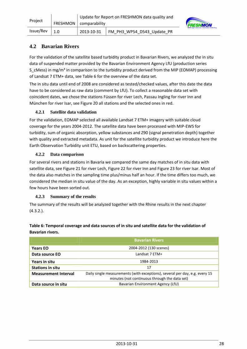
Table 6: Temporal coverage and data sources of in situ and satellite data for the validation of
Bavarian rivers.
Bavarian Rivers
Years EO 2004-2012 (130 scenes)
Data source EO Landsat 7 ETM+
Years in situ 1984-2013
Stations in situ 17
Measurement Interval Daily single measurements (with exceptions), several per day, e.g. every 15 minutes (not continuous through the data set)
Data source in situ Bavarian Environment Agency (LfU)

Project FRESHMON
Update for Report on FRESHMON data quality and
comparability
Issue/Rev 1.0 2013-10-31 FM_PH3_WP54_D543_Update_PR
2013-10-31 29
Figure 20. Overview of the all stations for Bavarian Rivers, stations selected for validation are
marked in dark red/ bold.
Figure 21. Comparison of Satellite derived turbidity and in situ measured Total Suspended Matter
for river Lech at station Füssen (47°33’57.32’’N, 10°42’1.06’’E).
Project FRESHMON
Update for Report on FRESHMON data quality and
comparability
Issue/Rev 1.0 2013-10-31 FM_PH3_WP54_D543_Update_PR
2013-10-31 30
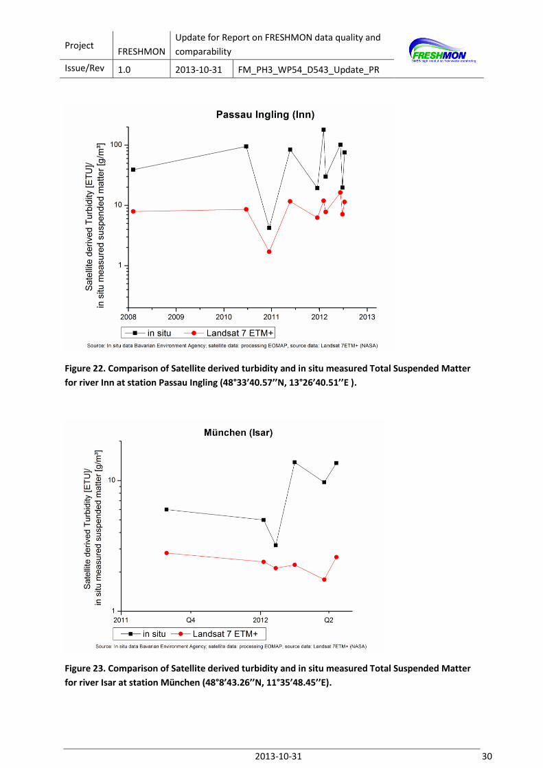
Figure 22. Comparison of Satellite derived turbidity and in situ measured Total Suspended Matter
for river Inn at station Passau Ingling (48°33’40.57’’N, 13°26’40.51’’E ).
Figure 23. Comparison of Satellite derived turbidity and in situ measured Total Suspended Matter
for river Isar at station München (48°8’43.26’’N, 11°35’48.45’’E).
Project FRESHMON
Update for Report on FRESHMON data quality and
comparability
Issue/Rev 1.0 2013-10-31 FM_PH3_WP54_D543_Update_PR
2013-10-31 31
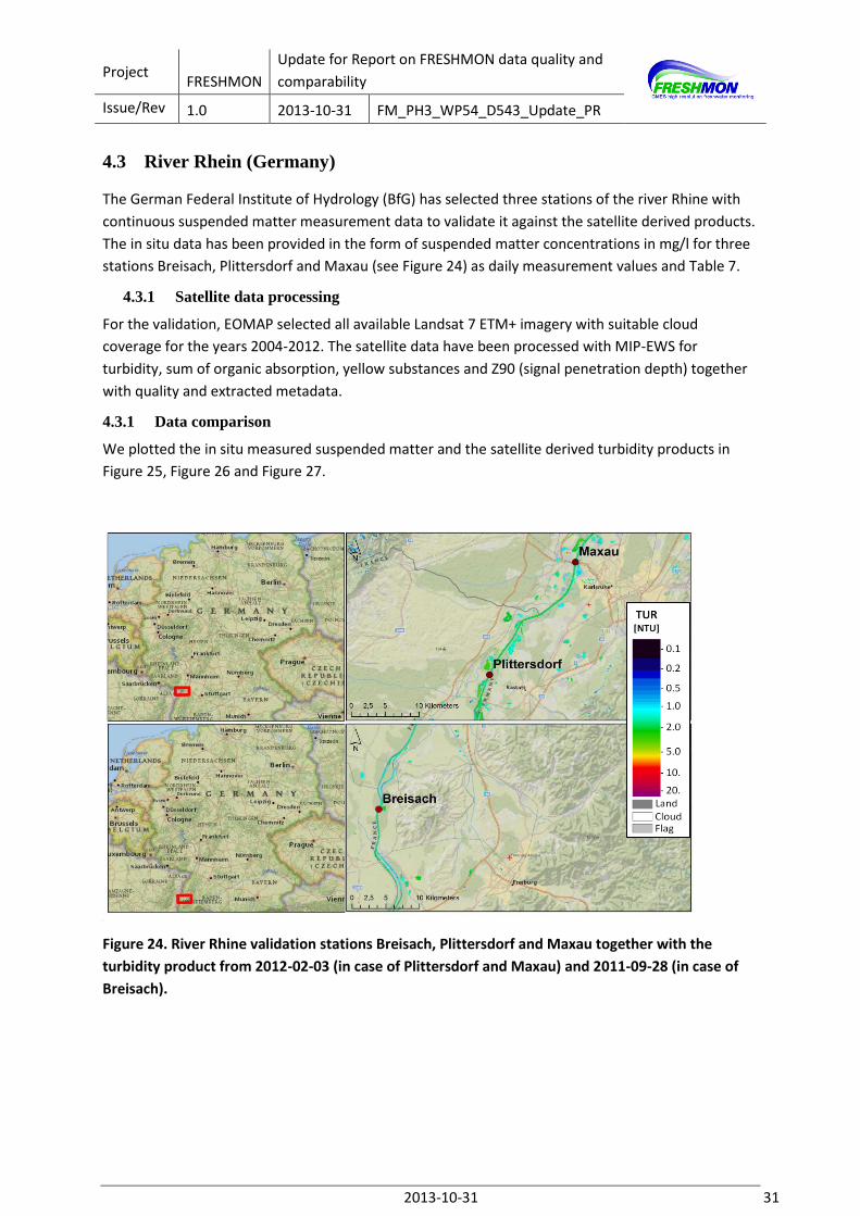
4.3 River Rhein (Germany)
The German Federal Institute of Hydrology (BfG) has selected three stations of the river Rhine with
continuous suspended matter measurement data to validate it against the satellite derived products.
The in situ data has been provided in the form of suspended matter concentrations in mg/l for three
stations Breisach, Plittersdorf and Maxau (see Figure 24) as daily measurement values and Table 7.
4.3.1 Satellite data processing
For the validation, EOMAP selected all available Landsat 7 ETM+ imagery with suitable cloud
coverage for the years 2004-2012. The satellite data have been processed with MIP-EWS for
turbidity, sum of organic absorption, yellow substances and Z90 (signal penetration depth) together
with quality and extracted metadata.
4.3.1 Data comparison
We plotted the in situ measured suspended matter and the satellite derived turbidity products in
Figure 25, Figure 26 and Figure 27.
n
Figure 24. River Rhine validation stations Breisach, Plittersdorf and Maxau together with the
turbidity product from 2012-02-03 (in case of Plittersdorf and Maxau) and 2011-09-28 (in case of
Breisach).

Project FRESHMON
Update for Report on FRESHMON data quality and
comparability
Issue/Rev 1.0 2013-10-31 FM_PH3_WP54_D543_Update_PR
2013-10-31 32
Table 7: Temporal coverage and data sources of in situ and satellite data for the validation of river
Rhine.
Rhine
Years EO 2004-2012 (72 scenes)
Data source EO Landsat 7 ETM+
Years in situ 1984-2011
Stations in situ 3
Measurement Interval Daily mean until July 2011
Data source in situ German Federal Institute of Hydrology (BfG)
Figure 25. Comparison of Satellite derived turbidity and in situ measured Total Suspended Matter
for river Rhine at station Maxau.

Project FRESHMON
Update for Report on FRESHMON data quality and
comparability
Issue/Rev 1.0 2013-10-31 FM_PH3_WP54_D543_Update_PR
2013-10-31 33
Figure 26. Comparison of Satellite derived turbidity and in situ measured Total Suspended Matter
for river Rhine at station Plittersdorf.
Figure 27. Comparison of Satellite derived turbidity and in situ measured Total Suspended Matter
for river Rhine at station Breisach.

Project FRESHMON
Update for Report on FRESHMON data quality and
comparability
Issue/Rev 1.0 2013-10-31 FM_PH3_WP54_D543_Update_PR
2013-10-31 34
4.3.2 Summary of the results
In situ data and satellite derived turbidity indicate the same temporal trends and dynamics for all
three stations in the different Bavarian rivers and for the river Rhine stations. Due to different
methodologies of the measures - satellite turbidity, in situ derived suspended matter (using again
different methodologies) – we observe quantitative differences, so each in situ methodology should
be related to always the same satellite derived ETU.
Figure 28 shows this when comparing different in situ stations with matching satellite derived
turbidity: The calibration to in situ measured suspended matter vary for some stations. This may be
due to different in situ methodologies, or also due to different optical backscattering properties (e.g.
varying particle size distributions) specific to the different locations. We furthermore expect that the
location of the in situ sampling point has a dominant impact for unsystematic difference: Locations
close to the shore (which is the case in most of the analyze in situ stations) or closer to the seafloor
are highly impacted by resuspension and localized hydrodynamic effects, and may not always
represent the values of the main river volume. Another methodological difference is the sampling
depth: The satellite based turbidity reflects the values close to the water surface (typically the first
30cm to 100cm in rivers), while the in situ sampling points are frequently deeper located.
4.3.1 User comments
The results have not been presented to the users so far, but will be discussed at the upcoming user
workshop in Munich on the 6th of November 2013.
Figure 28. Satellite derived turbidity vs. In Situ measured Total Suspended Matter for river Rhine
and Bavarian rivers.
Project FRESHMON
Update for Report on FRESHMON data quality and
comparability
Issue/Rev 1.0 2013-10-31 FM_PH3_WP54_D543_Update_PR
2013-10-31 35
4.4 Lakes in Mecklenburg-Vorpommern
4.4.1 In situ data
The validation in Mecklenburg-Vorpommern (North-East of Germany) has been performed for MERIS
water quality products and in situ measurements provided by the Ministerium für Landwirtschaft,
Umwelt und Verbraucherschutz Mecklenburg-Vorpommern, Abteilung 4. The in situ measurements
cover the years from 2003 – 2011 and are taken from different lakes. Figure 29 shows the area of
interest, while Figure 30 is zooming to the positions of the stations.
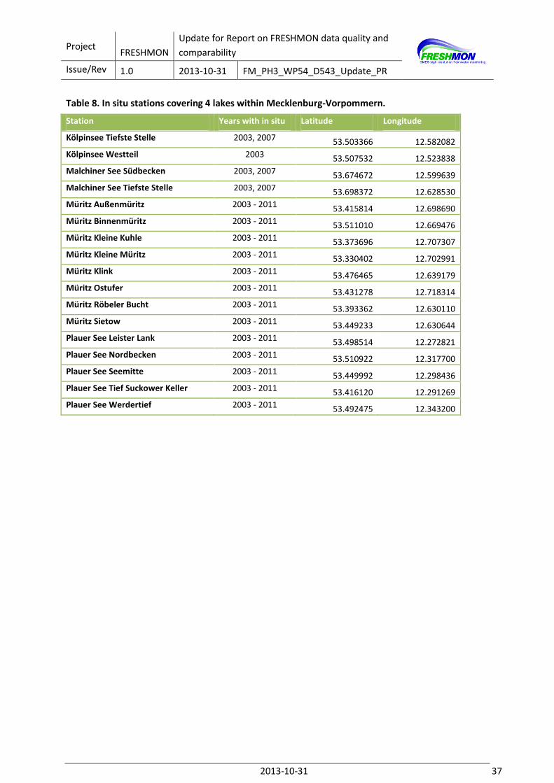
Table 8 lists the stations we received data from and the years they are covering. The data included
Secchi depths and chlorophyll concentration.
4.4.2 MERIS data
MERIS FR data have been processed with the FRESHMON processing chain at BC, including an
advanced pre-processing, water constituents retrieval with the FUB algorithm and a post-
processing/flagging for erasing invalid pixels. The processing has been performed on the calvalus
cluster for the archived MERIS data, only processing the pixels around the measurement stations.
4.4.3 Time Series Extraction & statistics
The chlorophyll concentration and KD values have been extracted around the stations using a 3x3
macro-pixel around the respective positions. The values within the macro pixels have been averaged
after the removal of invalid pixels and outliers. Subsequently, the time series have been plotted for
each station, sorted by lakes. Figure 32 demonstrates the resulting plots, which are presented in
chapter 4.4.4.3 for the different stations.
Furthermore, lakes statistics have been calculated. Here, averages of the data at the different
stations were calculated for the single years. Furthermore, the stations within one lake have been
compiled for the retrieval of a yearly average. For the in situ data, these were 5 to 6 measurements
per year, while the averages from the MERIS data have been received from up to 87 values, most of
them between 30 and 50 per year.
Match-up extraction of the exact measurement points provides the possibility to directly compare
the pixel and point values. The derived scatter plots supply a first guess of the agreement of data, but
should not be overestimated due to the constraints of comparing point and pixel data. Time
differences of in situ and MERIS where up to 4 hours.

Project FRESHMON
Update for Report on FRESHMON data quality and
comparability
Issue/Rev 1.0 2013-10-31 FM_PH3_WP54_D543_Update_PR
2013-10-31 36
Figure 29. Area of Interest covering the largest lakes in Mecklenburg-Vorpommern, North-East
Germany.
Figure 30. Position of in situ measurement stations of 4 lakes in Mecklenburg-Vorpommern;
Background map: NatGeo_World_Map - National Geographic, Esri, DeLorme, NAVTEQ, UNEP-
WCMC, USGS, NASA, ESA, METI, NRCAN, GEBCO, NOAA, iPC; image within the lakes: MERIS RGB
Image from 26.03.2007.
Project FRESHMON
Update for Report on FRESHMON data quality and
comparability
Issue/Rev 1.0 2013-10-31 FM_PH3_WP54_D543_Update_PR
2013-10-31 37
Table 8. In situ stations covering 4 lakes within Mecklenburg-Vorpommern.
Station Years with in situ Latitude Longitude
Kölpinsee Tiefste Stelle 2003, 2007 53.503366 12.582082
Kölpinsee Westteil 2003 53.507532 12.523838
Malchiner See Südbecken 2003, 2007 53.674672 12.599639
Malchiner See Tiefste Stelle 2003, 2007 53.698372 12.628530
Müritz Außenmüritz 2003 - 2011 53.415814 12.698690
Müritz Binnenmüritz 2003 - 2011 53.511010 12.669476
Müritz Kleine Kuhle 2003 - 2011 53.373696 12.707307
Müritz Kleine Müritz 2003 - 2011 53.330402 12.702991
Müritz Klink 2003 - 2011 53.476465 12.639179
Müritz Ostufer 2003 - 2011 53.431278 12.718314
Müritz Röbeler Bucht 2003 - 2011 53.393362 12.630110
Müritz Sietow 2003 - 2011 53.449233 12.630644
Plauer See Leister Lank 2003 - 2011 53.498514 12.272821
Plauer See Nordbecken 2003 - 2011 53.510922 12.317700
Plauer See Seemitte 2003 - 2011 53.449992 12.298436
Plauer See Tief Suckower Keller 2003 - 2011 53.416120 12.291269
Plauer See Werdertief 2003 - 2011 53.492475 12.343200
Project FRESHMON
Update for Report on FRESHMON data quality and
comparability
Issue/Rev 1.0 2013-10-31 FM_PH3_WP54_D543_Update_PR
2013-10-31 38
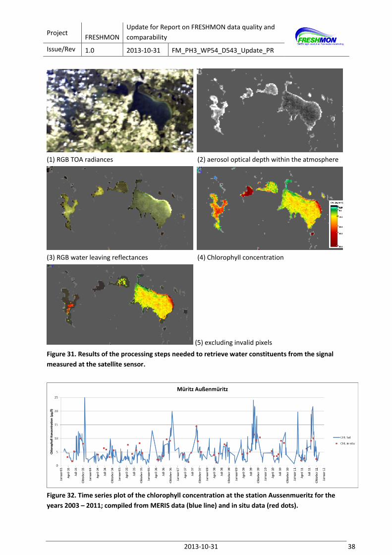
(1) RGB TOA radiances (2) aerosol optical depth within the atmosphere
(3) RGB water leaving reflectances (4) Chlorophyll concentration
(5) excluding invalid pixels
Figure 31. Results of the processing steps needed to retrieve water constituents from the signal
measured at the satellite sensor.
Figure 32. Time series plot of the chlorophyll concentration at the station Aussenmueritz for the
years 2003 – 2011; compiled from MERIS data (blue line) and in situ data (red dots).
Project FRESHMON
Update for Report on FRESHMON data quality and
comparability
Issue/Rev 1.0 2013-10-31 FM_PH3_WP54_D543_Update_PR
2013-10-31 39
4.4.4 Results
4.4.4.1 Match-Up statistics
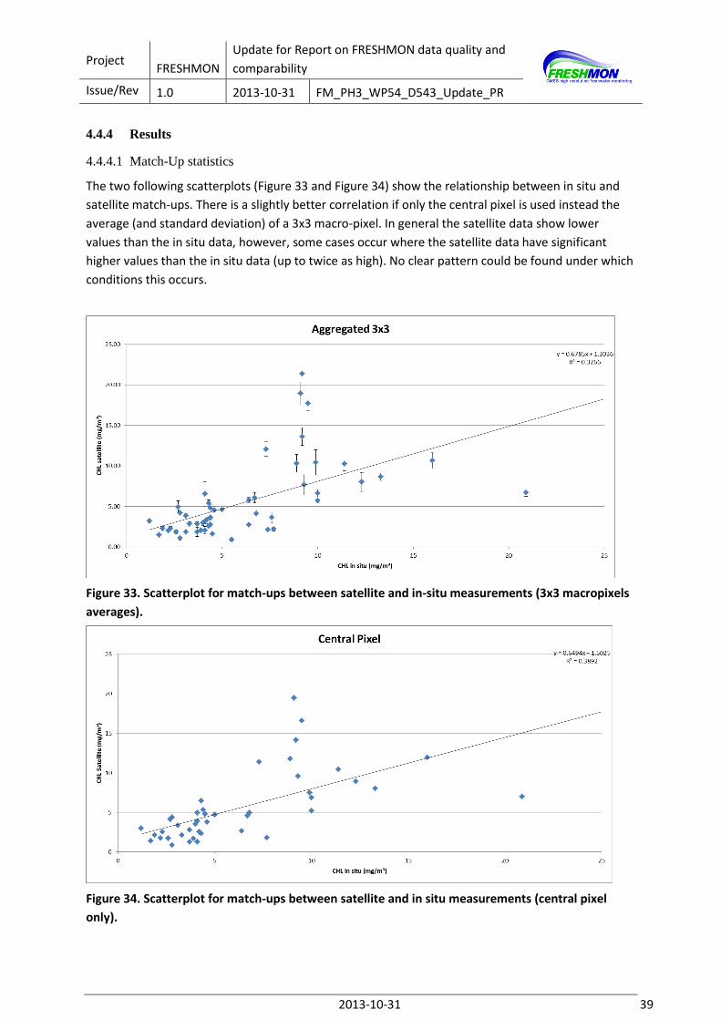
The two following scatterplots (Figure 33 and Figure 34) show the relationship between in situ and
satellite match-ups. There is a slightly better correlation if only the central pixel is used instead the
average (and standard deviation) of a 3x3 macro-pixel. In general the satellite data show lower
values than the in situ data, however, some cases occur where the satellite data have significant
higher values than the in situ data (up to twice as high). No clear pattern could be found under which
conditions this occurs.
Figure 33. Scatterplot for match-ups between satellite and in-situ measurements (3x3 macropixels
averages).
Figure 34. Scatterplot for match-ups between satellite and in situ measurements (central pixel
only).
Project FRESHMON
Update for Report on FRESHMON data quality and
comparability
Issue/Rev 1.0 2013-10-31 FM_PH3_WP54_D543_Update_PR
2013-10-31 40
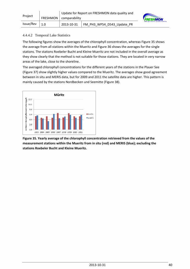
4.4.4.2 Temporal Lake Statistics
The following figures show the averages of the chlorophyll concentration, whereas Figure 35 shows
the average from all stations within the Mueritz and Figure 36 shows the averages for the single
stations. The stations Roebeler Bucht and Kleine Mueritz are not included in the overall average as
they show clearly that the method is not suitable for those stations. They are located in very narrow
areas of the lake, close to the shoreline.
The averaged chlorophyll concentrations for the different years of the stations in the Plauer See
(Figure 37) show slightly higher values compared to the Mueritz. The averages show good agreement
between in situ and MERIS data, but for 2009 and 2011 the satellite data are higher. This pattern is
mainly caused by the stations Nordbecken und Seemitte (Figure 38).
Figure 35. Yearly average of the chlorophyll concentration retrieved from the values of the
measurement stations within the Mueritz from in situ (red) and MERIS (blue); excluding the
stations Roebeler Bucht and Kleine Mueritz.

Project FRESHMON
Update for Report on FRESHMON data quality and
comparability
Issue/Rev 1.0 2013-10-31 FM_PH3_WP54_D543_Update_PR
2013-10-31 41
Figure 36. Comparison of the yearly averages of chlorophyll concentration at the different stations
within the Mueritz, in situ: red; MERIS: blue.
Figure 37. Yearly average of the chlorophyll concentration retrieved from the values of the
measurement stations within the Plauer See from in situ (red) and MERIS (blue).

Project FRESHMON
Update for Report on FRESHMON data quality and
comparability
Issue/Rev 1.0 2013-10-31 FM_PH3_WP54_D543_Update_PR
2013-10-31 42
Figure 38. Comparison of the yearly averages of chlorophyll concentration at the different stations
within the Plauer See, in situ: red; MERIS: blue.
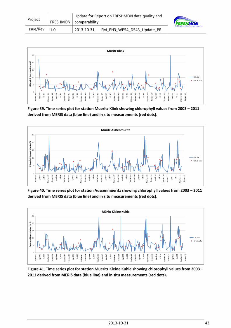
4.4.4.3 Time Series Plots
Mueritz
In total, there are eight measurement stations within the
Mueritz. T time series plots of four stations are shown below.
The map on the left is showing the position of the respective
stations. Best agreement between in situ and satellite
chlorophyll data can be seen for the stations Kleine Kuhle,
Außenmueritz, Mueritz Klink. An overall good agreement can
be seen in the yearly development as well as the absolute
levels of the chlorophyll concentration. The satellite data
provide a larger number of measurements, but also showing a
higher scatter of the data. The stations with good agreement
are located in the central area of the lake. For stations located
closer to the shoreline or within narrow areas of the lake, both
measurements do not agree. One example is the station Roebeler Bucht where only few chlorophyll
retrievals from MERIS are valid and show much too low values compared to the in situ
measurements. For the Station Mueritz Ostufer many data could be extracted from the satellite data
but showing a high scatter. This could be due to the fact that the station is located in an area where
bottom reflection might occur, due to water conditions. Therefore, the identification and excluding
of pixels with bottom reflection will be in the focus for future work.
Project FRESHMON
Update for Report on FRESHMON data quality and
comparability
Issue/Rev 1.0 2013-10-31 FM_PH3_WP54_D543_Update_PR
2013-10-31 43
Figure 39. Time series plot for station Mueritz Klink showing chlorophyll values from 2003 – 2011
derived from MERIS data (blue line) and in situ measurements (red dots).
Figure 40. Time series plot for station Aussenmueritz showing chlorophyll values from 2003 – 2011
derived from MERIS data (blue line) and in situ measurements (red dots).
Figure 41. Time series plot for station Mueritz Kleine Kuhle showing chlorophyll values from 2003 –
2011 derived from MERIS data (blue line) and in situ measurements (red dots).

Project FRESHMON
Update for Report on FRESHMON data quality and
comparability
Issue/Rev 1.0 2013-10-31 FM_PH3_WP54_D543_Update_PR
2013-10-31 44
Figure 42. Time series plot for station Mueritz Ostufer showing chlorophyll values from 2003 –
2011 derived from MERIS data (blue line) and in situ measurements (red dots).
Figure 43. Time series plot for station Roebeler Bucht showing chlorophyll values from 2003 – 2011
derived from MERIS data (blue line) and in situ measurements (red dots).
Plauer See
There are five monitoring stations within the Plauer See, while
suitable data could be extracted for 4 of them and only a few valid
measurements are available for station Werdertief.

Project FRESHMON
Update for Report on FRESHMON data quality and
comparability
Issue/Rev 1.0 2013-10-31 FM_PH3_WP54_D543_Update_PR
2013-10-31 45
Figure 44. Time series plot for station Plauer See Seemitte Keller showing chlorophyll values from
2003 – 2011 derived from MERIS data (blue line) and in situ measurements (red dots).
Figure 46. Time series plot for station Plauer See Suckower Keller showing chlorophyll values from
2003 – 2011 derived from MERIS data (blue line) and in situ measurements (red dots).
Figure 45. Time series plot for station Plauer See Nordbecken showing chlorophyll values from
2003 – 2011 derived from MERIS data (blue line) and in situ measurements (red dots).

Project FRESHMON
Update for Report on FRESHMON data quality and
comparability
Issue/Rev 1.0 2013-10-31 FM_PH3_WP54_D543_Update_PR
2013-10-31 46
Figure 47. Time series plot for station Plauer See Werdertief showing chlorophyll values from 2003
– 2011 derived from MERIS data (blue dots) and in situ measurements (red dots).
4.4.5 Conclusions
The above demonstrated comparisons between in situ measurements and satellite based retrieval of
chlorophyll concentration shows the overall good agreement of both methods – where applicable -
and the complementarity of the techniques. The opportunities that can be retrieved from a
combined usage and analysis would provide a very valuable data set for lake monitoring.

Project FRESHMON
Update for Report on FRESHMON data quality and
comparability
Issue/Rev 1.0 2013-10-31 FM_PH3_WP54_D543_Update_PR
2013-10-31 47
5 Conclusions
5.1 Quality of in situ data
SYKE:
In Finland, the Chl-a in situ data came from the national monitoring programme. Since the analyses
are done in certified laboratories, we assume the quality of in situ data to be high. However, the
locations of the stations are not always optimal for EO validation and simultaneous match-ups are in
practice only possible at automatic stations.
EOMAP:
The situ data differs a lot in terms of temporal resolution, e.g. daily measurements vs. two-weekly or
monthly measurements. Furthermore, we receive either daily mean values or exact measurement
times as input, which have to be compared. For one example we only received non-calibrated data
from a specific date onwards, therefore the validation has to be considered with caution. In a lot of
cases, we have not found enough matching dates to validate the products in an effective way. As we
have demonstrated in D54.3, the time difference can play an important role in the comparability of
the measurements.
BC:
The in situ data and the procedure of sampling are dedicated for the monitoring requirements of
Mecklenburg-Vorpommern. The sampling was not dedicated to be suitable for the validation of
satellite data. While using these data for validation, we perform a validation fit of purpose showing
the users how the satellite derived chlorophyll values agree with their monitoring measurements.
5.2 Quality of satellite products
SYKE:
According to the validation results the MERIS Chl-a product works well in non-humic lakes. In humic
lakes the EO method underestimates the concentrations. The magnitude of the effect is still unclear
and this caused some concerns with the users. The effects of CDOM on Chl-a estimation will be
studied further in the GLaSS project.
The limited resolution of MERIS (300 m) is a problem as it cannot be used with small lakes where the
information needs are the largest.
The water depth products performed well for depths less than 2 to 3 m.
EOMAP:
For the high resolution products, the results are comparable with the moderate resolution products.
Therefore, the satellite product can –again- be considered as a harmonized product, independent
from the sensor resolution.
The number of validated Landsat 7 ETM+ images was limited. But the satellite products reflect the
temporal trends and dynamics of the in situ measured suspended matter quite well. With the launch

Project FRESHMON
Update for Report on FRESHMON data quality and
comparability
Issue/Rev 1.0 2013-10-31 FM_PH3_WP54_D543_Update_PR
2013-10-31 48
of the new sensor Landsat 8 in February 2013 and the upcoming launch of the Sentinel 2, the number
and hence the temporal resolution of suitable sensors in this spatial and spectral resolution class
increases significantly.
BC:
The processing of the MERIS products has been performed with the FRESHMON processing chain
which is based on the FUB processor without any local adjustment or calibration. Thus, the good
agreement to the in situ data is very promising and the processing seems to be very suitable for
these kind of lakes. The spatial resolution of the data is the limiting factor and only stations with a
certain distance to land were suitable for the comparison. On the other hand, the high temporal
resolution of the MERIS data provides very valuable additional information for monitoring aspects
and / or scientific questions.
5.3 Quality of data from in situ devices
The quality of data from in situ devices was not included in this update.

Project FRESHMON
Update for Report on FRESHMON data quality and
comparability
Issue/Rev 1.0 2013-10-31 FM_PH3_WP54_D543_Update_PR
2013-10-31 49
6 Validation lessons learnt
Important issues to take into account when comparing satellite and in situ measurements are:
Qualitative temporal trends and dynamics are more in focus than quantitative comparisons
of values when generated with different methodologies. This is mainly due to the lack of
simultaneous match-ups.
Possible time coincidence of the measurements in areas with highly variable conditions, e.g.
rivers or river inflows, is highly recommended when comparing same day measurements.
Location of the sampling stations, e.g. near the shore, can influence the results.
Different sampling depths occur in most cases when comparing satellite with in situ
measurements.
Feasibility check of suitable images (turbidity, atmospheric conditions) for water depth
processing.
Pixel wise quality control (the quality levels of data points in result images are indicated with
e.g. different symbols) of the satellite product plays an important role for the validation.
Temporal vs. spatial resolution needs to be demonstrated to the users and the advantages/
disadvantages needs to be discussed especially with respect to their requirements.
Further aggregation of products may bring the products closer to the requirements of the
users and the validation results also are less sensitive to single pixel to point comparisons.
In situ data which would follow the recommendations for validation purposes are not always
available. Routine in situ data is often acquired with different focus. Nevertheless, our
validation activities show that it is possible to compare the two data sources in useful way.

Project FRESHMON
Update for Report on FRESHMON data quality and
comparability
Issue/Rev 1.0 2013-10-31 FM_PH3_WP54_D543_Update_PR
2013-10-31 50
References
Albert, A. and Mobley, C.D., “An analytical model for subsurface irradiance and remote sensing
reflectance in deep and shallow case-2 waters,” Optics Express 11(22), 2873-2890 (2003)
Dekker, A.G. and Peters, S.W.M., The use of the Thematic Mapper for the analysis of eutrophic lakes:
A case study in The Netherlands. International Journal of Remote Sensing, vol. 14, no. 5, pp. 799-821,
1993.
Gitelson, A., Garbuzov, G., Szilagyi, F., Mittenzwey, K-H., Karnieli, K., and Kaiser, A., Quantitative
remote sensing methods for real-time monitoring of inland waters quality. International Journal of
Remote Sensing, vol. 14, no. 7, pp. 1269-1295, 1993.
Kallio, K. 2006. Optical properties of Finnish lakes estimated with simple bio-optical models and
water quality monitoring data. Nordic Hydrology 37: 183-204.
Lyzenga, D. R. 1978. Passive remote sensing techniques for mapping water depth and bottom
features. Applied Optics 17: 379-383.
Ohlendorf, S. , Müller, A. Heege, T., Cerdeira-Estrada, S. Kobryn, H.T. (2011): "Bathymetry mapping
and sea floor classification using multispectral satellite data and standardized physics-based data
processing", Proc. SPIE 8175, 817503; doi:10.1117/12.898652
Stumpf, R. P. & Holderied, K. 2003. Determination of water dept with high-resolution satellite
imagery over variable bottom types. Limnology and Oceanography 48(1-2): 547-556.