wp/21/ - international monetary fund

WP/21/10

Bank Balance Sheets and External Shocks in Asia: The Role of FXI, MPMs and CFMs

by Zefeng Chen, Sanaa Nadeem, and Shanaka J. Peiris

IMF Working Papers describe research in progress by the author(s) and are published to elicit comments and to encourage debate. The views expressed in IMF Working Papers are those of the author(s) and do not necessarily represent the views of the IMF, its Executive Board, or IMF management.

©International Monetary Fund. Not for Redistribution

© 2021 International Monetary Fund WP/21/10

IMF Working Paper

Asia and Pacific Department

Bank Balance Sheets and External Shocks in Asia: The Role of FXI, MPMs and CFMs

Prepared by Zefeng Chen, Sanaa Nadeem, and Shanaka J. Peiris

Authorized for distribution by Lamin Leigh

January 2021

Abstract

In emerging Asia, banks constitute the dominant source of financing consumption and investment, and bank balance sheets comprise large gross FX assets and liabilities. This paper extends the DSGE model of Gertler and Karadi (2011) to incorporate these key features and estimates a panel vector autoregression on ten Asian economies to understand the role of the banking sector in transmitting spillovers from the global financial cycle to small open economies. It also evaluates the effectiveness of foreign exchange intervention (FXI) and other macroeconomic policies in responding to external financing shocks. External financial shocks affect net external liabilities of banks and the exchange rate, leading to changes in credit supply by banks and investment. For example, a capital outflow shock leads to a deprecation that reduces the net worth and intermediation capacity of banks exposed to foreign currency liabilities. In such cases, the exchange rate acts as shock amplifier and sterilized FXI, often deployed by Asian economies, can help cushion the economy. By contrast, with real shocks, the exchange rate serves as a shock absorber, and any FXI that weakens that function can be costly. We also explore the effectiveness of the monetary policy interest rate, macroprudential policies (MPMs) and capital flow management measures (CFMs).

JEL Classification Numbers: E32, E44, F32, F41

Keywords: Capital flows, bank balance sheets, foreign exchange intervention, macroprudential policy, capital flows measures

Author’s E-Mail Address: [email protected], [email protected], [email protected]

IMF Working Papers describe research in progress by the author(s) and are published to elicit comments and to encourage debate. The views expressed in IMF Working Papers are those of the author(s) and do not necessarily represent the views of the IMF, its Executive Board, or IMF management.


Table of Contents

Abstract ..................................................................................................................................... 2

I. Introduction ........................................................................................................................... 4

II. The Role of Bank Balance Sheets in Emerging Asia: Empirical Evidence ......................... 8

III. Model ................................................................................................................................ 13

A. Household ...................................................................................................................... 13

B. Producers ........................................................................................................................ 14

Non-traded Good ............................................................................................................ 14

Capital Good ................................................................................................................... 16

C. Banks .............................................................................................................................. 17

Banker’s optimal choice ................................................................................................. 18

Aggregation..................................................................................................................... 19

D. Foreign Investor ............................................................................................................. 19

E. Government .................................................................................................................... 20

Monetary Policy .............................................................................................................. 20

Fiscal Policy .................................................................................................................... 20

Foreign Exchange Intervention ....................................................................................... 20

F. Market Equilibrium ........................................................................................................ 20

IV. Calibration ........................................................................................................................ 21

A. Capital Flow Shock ........................................................................................................ 21

B. Productivity Shock ......................................................................................................... 22

V. Alternative Policies ............................................................................................................ 23

A. Capital Flow Measures (CFMs) ..................................................................................... 23

B. Augmented Monetary Policy ......................................................................................... 24

C. Macroprudential Measures ............................................................................................. 24

D. Comparison Across Policies .......................................................................................... 25

E. Optimal Policy ................................................................................................................ 26

VI. Conclusion ........................................................................................................................ 27

Annex I. Summary Statistics................................................................................................... 29

Annex II: Panel VAR Estimates ............................................................................................. 30

Annex III. Panel VAR Impulse Response Functions.............................................................. 31

Annex IV. Schematic Description of Model ........................................................................... 35

VII. References ....................................................................................................................... 40


Underline

4

I. INTRODUCTION1

For small open economies that are increasingly integrated with the global economy, the international financial cycle, with its large and volatile cross-country capital flows, has become a vital consideration.2 Indeed, for emerging Asia, the substantial trade and financial linkages that have supported the region’s robust growth may also constitute a source of risk. Since the Global Financial Crisis (GFC), large surges in liquidity and a search for yield drove capital flows to emerging markets, notably in Asia (see IMF 2019a), together with sharp declines hand-in-hand with risk-off sentiment, such as the 2013 Taper Tantrum and the 2020 coronavirus pandemic. Such swings of capital—surges and sudden stops—can have disruptive macrofinancial consequences (Bruno and Shin 2015, Cechetti et al. 2020, Gelos et al. 2019). Thus, a central question is what makes some emerging market economies (EMs) more vulnerable to the effects of capital flows than others? An understanding of the key transmission channels through which the global financial cycle is propagated—or insulated against—in an emerging economy can bear important lessons for policymakers. In many Asian economies, banks form the central pillar of the financial system serving as the dominant source of financing for investment and consumption.3 A notable feature of these banking systems is that gross foreign assets and liabilities are sizeable, reflecting the region’s considerable trade and financial flows (Figure 1). Several Asian EMs maintain large net foreign asset positions, with gross foreign assets above foreign liabilities (Figure 2); foreign assets tend to be more volatile than liabilities, and both are more volatile in Asian EMs than in advanced economies (AEs) (Annex I). One rationale behind these holdings of FX assets by EM banks could be that such assets help ease collateral constraints to access foreign funding, particularly in times of stress, providing a cushion against foreign funding shocks. Given the rising importance of dollar-invoicing, non-US banks may still have limited access to FX deposits, and may have to rely on US wholesale funding market which can in many cases be volatile and dependent on financial conditions in the domestic economy (IMF 2019b). Given these features, bank balance sheets can serve as an important transmission mechanism for propagating external shocks to Asian economies. Indeed, in many Asian EMs, FX liabilities of banks are large when compared to corporates (Figure 3). External shocks, such as funding and exchange rate shocks, can affect the size, cost, and mix of banks’ balance sheets, which could in turn affect the amount of credit extended by banks to the private sector, and thereby—given banks’ dominant role in financing—investment and output. For Asia, whereas several transmission channels have been documented, such as corporate balance sheets and the price competitiveness of exports, and their effect on credit, investment, and growth, there is less evidence on the role of bank balance sheets.

1 This paper has benefited from feedback received from Andrew Berg, Davide Furceri, Nobuhiro Kiyotaki, Lamin Leigh, Machiko Narita, Jonathan Ostry, and seminars at the IMF (Asia Pacific Department (APD) and Internal Capacity Development (ICD) department) and Stanford University. 2 See for example, Lane and Milesi Ferretti (2007), and Avdjiev, Hardy, Kalemli-Ozcan and Serven (2018). 3 At end-2017, for 13 Asian economies (6 advanced (Australia, Hong Kong, Japan, Korea, New Zealand and Singapore) and 7 emerging (China, India, Indonesia, Malaysia, Philippines, Thailand, and Vietnam)), bank assets to GDP comprised an average of 168 and 102 percent of GDP respectively (World Bank Global Financial Development Database).


5

A second—and highly debated—question centers on the optimal policy response by EMs to these large and volatile capital flows. As noted in IMF 2019a, Asian economies have used a variety of policy instruments to target multiple objectives. This could reflect a landscape shaped by increasing financial integration, which has introduced new sources of shocks to EMs. Considerations of the international financial cycle and its spillovers can alter the objective functions of policymakers, including by introducing financial stability among its objectives (see Blanchard, Adler, and de Carvalho Filho 2015). This can generate new tradeoffs between different macroeconomic objectives and policies, thereby motivating policymakers to use a combination of instruments given the circumstances, such as foreign exchange intervention (FXI), macroprudential measures (MPMs) and capital flows measures (CFMs) in addition the monetary policy interest rate, as opposed to the mix generally suggested in standard monetary policy frameworks (Rey, 2018; Miranda-Agrippino and Rey, 2019; Obstfeld, Ostry and Qureshi 2019; Basu et al. 2020).

Figure 1: Foreign Assets and Liabilities of Banks in Select Asian Economies Foreign assets, as a share of GDP, 2001q4-2019q4 Foreign liabilities, as a share of GDP, 2001q4-2019q4

Source: Haver, IMF Monetary and Financial Statistics Database, authors’ calculations.

Figure 2: Banks' Foreign Assets as a Share of Foreign Liabilities

Figure 3: FX Liabilities of Financial and Nonfinancial Corporates, 2018 (percent of GDP)

Note: Average over period. Data for New Zealand available from 2013m3. Source: Haver, IMF Monetary and Financial Statistics Database, authors’ calculations.

Source: BIS, staff calculations


6

With these questions in mind, the overarching objective of this paper is to develop a framework to understand the role of the banking sector as a transmission channel for external shocks and thereby inform macroeconomic policy choices. First, we estimate a panel vector autoregression (VAR) following Abrigo and Love (2015) for ten Asian economies to explore the role of bank balance sheets in propagating external shocks. We use a panel VAR specification as it can better address the endogeneity between variables while benefiting from the cross-country variation in a panel setting. We consider two kinds of shocks: external financial shocks and real shocks. For the former, as a proxy for the global financial cycle, we consider an exogenous US monetary policy shock as in Albrizio et al. (forthcoming). For the latter, we consider shocks to foreign demand and productivity. We also estimate the panel VAR for two subsamples, advanced and emerging Asian economies to capture the differences in financial sector structure and depth between these two groups. Empirical analysis on Asia outside of Japan, Australia and New Zealand has been limited; similarly, most recent work has focused on the impact of such shocks on financial rather than macroeconomic variables (see Hong et al. 2019, IMF 2019a, IMF 2019b). Overall, our empirical analysis informs our understanding of whether and why the bank balance sheet channel matters, thereby leveraging the Asian experience for broader lessons for other EMs. Tracing the transmission of external shocks—in this case through banks—is key to informing policy. For small open economies, the exchange rate is generally regarded as the first line of defense against external financial shocks (Kalemli-Ozcan 2019). For example, a depreciation in response to capital outflows makes exporting goods cheaper, improving international competitiveness and boosting economic activity (competitiveness channel). However, the short-term response of trade flows to exchange rate movements can be asymmetric, reducing imports but exerting little immediate effect on exports due to trade pricing in dominant currencies (Gopinath 2015 and IMF 2019b). Further, exchange rate fluctuations can in some cases aggravate corporate vulnerabilities and discourage investment, especially in the presence of FX liabilities (corporate financial channel). Another channel (the bank lending channel) operates in the same direction: a depreciation can weaken bank balance sheets and impair their capacity to lend and reduce firms’ access to finance (Bruno and Shin 2015). More broadly, in acting as a shock amplifier rather than a shock absorber, exchange rate movements can sharpen the tradeoff between price stability and financial stability (Aoki et al. 2018). Our panel VAR finds evidence for the exchange rate amplifying shocks through the bank lending channel, suggesting that a capital outflow shock leads to a depreciation of the currency, which reduces the net worth and intermediation capacity of banks that have foreign currency liabilities. This reduces the extension of credit by banks to the private sector and thereby investment. To further explore these dynamics, this paper extends a canonical New-Keynesian DSGE model of a small open economy (Gertler and Karadi 2011) with a banking sector that can access both domestic and foreign funds. We use this to investigate the transmission of external real and financial shocks to the economy and the relative performance of alternative macro-financial policies (namely the monetary policy interest rate, FXI, MPMs and CFMs). As in Aoki et al. (2018), in the banking sector, home deposits are denominated in the home currency while foreign borrowing is denominated in foreign currency. In addition, this paper allows banks to hold FX-denominated assets (e.g. US Treasuries) as a safe asset which allows them to more readily access foreign funding, a key feature observed in the data for Asian EMs. Non-tradable goods prices are


7

subject to adjustment costs as in Rotemberg (1982) while traded goods are priced in foreign currency (U.S. dollar invoicing) consistent with Gopinath (2015). As in standard New-Keynesian models, a decline in the policy interest rate increases consumption and investment, depreciates the currency and boosts exports over time. However, banks’ balance sheets are an additional channel through which the real economy is impacted by shocks, real or financial, and the resulting changes in bank credit affect domestic investment and output. In comparison to Aoki et al. 2018, to capture particularly relevant features of Asian EMs, we introduce US dollar invoicing, allow for an incentive for banks to hold foreign assets as safe assets, and introduce the FXI as an additional policy instrument. In comparing the different policy responses, this model contributes to the literature on the appropriate mix and effectiveness of monetary policy interest rate, MPMs, FXI, and CFMs for small open economies in managing shocks. Of main interest to Asian EMs, this paper contributes to the emerging literature on the effectiveness of FXI in securing external stability and responding to external shocks. Despite the popularity of FXI in practice, theoretical work to guide its implementation is only now emerging while empirical evidence has on the effectiveness of FXI has been mixed (see Basu et al. 2020, Liu and Spiegel 2015; Cavallino 2019). Some work finds limited use of FXI for a broad sample of countries (Chamon et al. 2019, Brendao-Marques et al. 2020); while a more focused look at Asian EMs highlighting these economies’ particular financial frictions finds that FXI can be effective for financial shocks (Deb et al. 2020). This paper takes a closer look at the rationale for FXI—in combination with other policies—in Asian EMs in response to the global financial cycle, following a number of studies on EMs (see Benes et al. 2013; Escude 2013; Ostry, Ghosh, and Chamon 2012). Another key question is the role of MPMs, specifically, whether they can help ease the tension between monetary and financial stability objectives. Some of the growing literature suggests the use of monetary policy interest rate to lean against the wind (LATW) has limited effectiveness for small open economies, as such measures can trigger movements in capital flows and worsen the tradeoff between macro- and financial stability (Unsal 2013, Medina and Roldos 2014, Aoki et al. 2018; Sahay and others 2014; Menna and Tobal 2017); others show gains from attaching a weight on the real exchange rate under country risk-premia shocks (Mimir and Sunel 2015). Using the policy interest to LATW alone may be insufficient to appropriately target financial vulnerabilities, making MPMs a critical complement (see Shin 2013 and Chung et al. 2014). On the empirical side Brendao-Marques et al. 2020 find evidence for the effectiveness of MPMs in EMs, and for Asia, a few papers assess the role of loan-to-value ratios (Oktiyanto and others 2014) and counter-cyclical capital requirements (Corbacho and Peiris 2018, Ghilardi and Peiris 2016); Alam et al. (2019) provide a cross-county review of MPMs used. In this paper to highlight this tradeoff, we consider a tax on foreign borrowing and differential reserve requirements on foreign borrowing by banks, which may constitute CFMs and/or MPMs. Overall, this paper seeks to contribute to the literature on the optimal combination of policies used by EMs to manage external shocks by developing a model exploring the role of banks, which is calibrated to Asian EMs to provide quantitative policy assessments in a realistic policy setting. A panel VAR finds evidence for the role of bank balance sheets in propagating external shocks in Asian EMs relative to AEs, where the exchange rate can act as a shock amplifier rather than a shock absorber. We then study the role of FXI, MPMs (a reserve requirement on bank


8

foreign liabilities), and CFMs (a cyclical tax on foreign currency borrowing) and their interaction with the policy interest rate. Model simulations suggest that economies similar to Asian EMs, the efficacy of FXI depends upon the relative importance of financial versus non-financial shocks. If external financial shocks are important, the use of FXI can improve overall welfare. FXI can mitigate sharp exchange rate declines in response to such shocks, preserving bank balance sheets, credit and investment. In contrast, any counterbalancing increase in competitiveness is relatively muted due to dollar price invoicing. If non-financial shocks are more important, a standard Taylor rule improves welfare relative to other policy instruments. We also find there can be welfare gains from cyclical macroprudential policies and CFMs as such measures could help stabilize the bank balance sheet and external exposures respectively, allowing room for monetary policy to focus on the more traditional macro stability objective, leading to welfare gains.

II. THE ROLE OF BANK BALANCE SHEETS IN EMERGING ASIA: EMPIRICAL EVIDENCE

We estimate a panel vector autoregression (VAR) as in Abrigo and Love (2015) to assess the effect of external shocks and the role of bank balance sheets in propagating these shocks on key macroeconomic variables in Asian economies. The panel VAR uses system-GMM estimators to examine the relationship between external financing shocks, banks’ foreign assets and liabilities, the real exchange rate, credit and investment. We estimate the panel VAR using quarterly data from 2002Q1 to 2019Q4 for ten Asian economies: four advanced (Australia, Korea, Japan, and New Zealand) and six emerging (China, India, Indonesia, Malaysia, the Philippines, and Thailand), using the following specification:

𝑌𝑖𝑡 = 𝑌𝑖𝑡−1𝐴1 + 𝑌𝑖𝑡−2𝐴2 + ⋯ + 𝑌𝑖𝑡−𝑇𝐴𝑇 + 𝑋𝑖𝑡𝐵 + 𝑢𝑖𝑡 + 𝑒𝑖𝑡 (1)

where 𝑌𝑖𝑡 is the vector of endogenous variables: growth in foreign assets, growth in foreign liabilities, change in the real exchange rate, growth in credit to the private sector, and growth in real investment; 𝑋𝑖𝑡 is a vector of exogenous variables (US GDP growth, inflation, terms of trade, and an external financing shock); 𝑢𝑖𝑡 and 𝑒𝑖𝑡 are dependent variable specific fixed effects and idiosyncratic errors respectively.4 All growth rates are quarterly growth rates. We fit a second-order VAR (𝑇 = 2) as it generally yields smaller MBIC, MAIC, and MQIC values, following Andrews and Lu (2001). To better investigate transmission channels of bank balance sheets and as an added robustness check, we also estimate the model at a monthly frequency over the period 2001M12 and 2020M2, using foreign assets and liabilities, the real exchange rate, credit, and the index of industrial production (IIP) as the real variable in lieu of investment due to data availability at this frequency.5

4 Data on banks’ gross foreign (nonresident) assets (claims) and liabilities and credit to the private sector are taken from the depository corporations (ODC) survey from the IMF’s Monetary and Financial Sector database, where they are available at a monthly and quarterly frequency; data on ODC FX assets and liabilities for China and India are from Haver. GDP and investment growth is calculated as the change in real output and gross fixed capital formation respectively from Haver. The real exchange rate is the quarter on quarter change in the CPI-based REER from the IMF Information Notice System database. 5 We cannot use the monthly model to assess the effect of exogenous external shocks, which are only available at a quarterly frequency, hence we limit its use to a robustness check. The specification has a 12-period lag.


9

We expect bank balance sheets to serve as an amplification mechanism for different types of external shocks. First, for a positive external financial shock (such as a loosening in global financial conditions), we expect bank external borrowing and deposits to rise; this expansion in the banks’ balance sheets as well as a real exchange rate appreciation (which further relaxes banks’ funding constraints) together drive increased credit extension by banks and investment by firms in the economy over time. Second, for a positive external real shock, such as an increase in the U.S. GDP growth rate (foreign demand) or an improvement in the terms of trade, we expect a similar relaxation in banks’ collateral constraints through higher foreign funding (either by increased foreign investment resources or improved sentiment), which would raise bank lending and investment in the domestic economy. It would be instructive to assess the relative importance of these two types of shocks; it would appear that in EMs, the link between financial shocks to bank balance sheets is stronger through valuation effects from the exchange rate, thereby having a more pronounced effect on credit and investment. We estimate equation (1) and generate impulse response functions (IRFs) in response to shocks to different endogenous and exogenous variables; confidence bands are estimated using Gaussian approximation based on 200 Monte Carlo draws from standard errors of the estimated panel VAR. We order the variables based on a Cholesky decomposition (Sims 1980), as real exchange rate, foreign liabilities, foreign assets, credit and investment. The IRFs are robust to alternate orderings of foreign assets and liabilities. We estimate (1) at a quarterly frequency, and estimation at the monthly frequency confirms the direction of these findings. External financing shocks We consider several measures of external financing shocks. First, we use the exogenous monetary policy variable as in Albrizio et al. (forthcoming);6 we prefer this over the VIX, a widely used measure of global risk aversion, as it may itself be endogenous.7 We find that a negative shock (tightening of external financial conditions) reduces foreign liabilities and assets, decreases the supply of bank credit, and lowers investment for both advanced and emerging Asia (Figure 4a and Annex II). We also test several alternative measures of external financial shocks, the excess bond premium as in Gilchrist and Zakrajsek 2012, the VIX, and the US federal funds rate with similar results (Annex III.2). This result is supported using the monthly panel VAR using the VIX and the US federal funds rate (FFR) as proxies for the external financial shock (Annex III.1).8 External real shock We compare the above external financial shocks to a real foreign demand shock, proxied by US growth. We find that an increase in US growth increases foreign liabilities and assets in domestic banks, as foreign investors have more resources to invest, but leads to a small depreciation in the real exchange rate (given the appreciation in the US dollar), leading to a net lower increase in credit than suggested by the financial conditions scenario above (Figure 4b). We also use the

6 The monetary policy shock is estimated using the residual of the one-year government bond rate regression with the 30-min changes of the one-month ahead Fed funds futures around FOMC announcements. 7 When using the VIX as the financial shock variable, we find that it has a less significant effect via bank balance sheets (particularly for advanced economies), though with a stronger magnitude of an effect on the exchange rate and credit. 8 The monthly VAR supports in the contraction in the balance sheet due to a shock to the VIX and FFR, and whereas the effect on IIP is in the same direction has investment, it has large error bands.


10

terms of trade as an additional external real shock, with similar directional results, with the exception of the real exchange rate, where a positive terms of trade shock leads to a domestic real exchange rate appreciation, strengthening the increase in credit, but with lower overall level of significance (Annex III.2). Foreign liabilities As foreign liabilities are likely a key transmission channel of external financing shocks in EM Asia, we focus on direct foreign bank funding shocks to evaluate the amplification through the banking system. A positive shock to foreign liabilities (proxying a capital inflow) raises foreign assets and leads to a real exchange rate appreciation and an increase in credit to the private sector and investment to GDP (Figure 4c). Given the larger size of foreign liabilities in advanced than in emerging Asia, we find a more significant effect on bank assets and the exchange rate in these economies. In EM Asia, the effect of a foreign funding shock on the exchange rate is less clear, which could reflect the use of policies to mitigate movements in the exchange rate. The monthly panel VAR supports the increase in foreign assets and credit from higher foreign liabilities (Annex III.1). Foreign assets We next test a positive shock to foreign assets. Here, there is some evidence of an increase in foreign liabilities, albeit with a lag, followed by credit and investment, particularly for the EM subsample. This suggests an additional amplification channel through bank balance sheets, through which banks have an incentive to hold foreign “safe” assets such as US Treasuries. Holding such safe assets may encourage foreign deposits and funding, where foreign investors believe such banks are more likely to meet external obligations, as well as provide a buffer against foreign funding shocks, thereby loosening banks’ financing constraints. This could explain the observation in the data where several Asian economies hold foreign assets above foreign liabilities, particularly in times of stress. Real exchange rate Another transmission channel is through the real exchange rate itself. The exchange rate affects bank balance sheets through valuation effects (with a real appreciation relaxing funding constraint, as in the positive foreign liabilities shock above), but also directly to the economy, say via competitiveness or corporate balance sheets. We find that controlling for the bank balance sheet, the real exchange rate appreciation affects credit but with wider confidence intervals on foreign assets and liabilities (Figure 4e). Splitting the sample between Asian EMs and advanced economies generally reveals that the role of the exchange rate on bank balance sheets is stronger for EMs than for advanced economies. A forecast error variance decomposition for foreign assets and liabilities, the real exchange rate, credit, and investment highlight the relative important role of financial versus real variables. As highlighted in Figure 5 banking financial shocks (such as capital inflows proxied by foreign liabilities and assets), and the external financing shocks more directly have a larger contribution to the forecast variance than real shocks (such as US growth and terms of trade). It also appears that the real exchange rate responds to both real and financial shocks but seems to be more susceptible to financial shocks in EM Asia, though one would need to consider the potential role of policies that could temper movements in the exchange rate to make a definite conclusion. This


11

could suggest that the bank balance sheet channel serves as a stronger shock amplifier for financial shocks than nonfinancial shocks. In an additional robustness check, we introduce into the specification nonfinancial corporate FX borrowing to assess the importance of bank balance sheet channel controlling for corporate balance sheets (Annex II.3). It could be that the effect on credit and investment stems from corporate activity independent of the increased lending via banks due to the loosening of the latter’s financing constraints. Here, we find that controlling for corporate FX debt, the bank balance sheet channels remain significant under a capital inflow shock, while corporate FX debt has large standard errors. Under the real shocks as well, corporate FX debt has the expected signs, but has lower significance. This would suggest that the bank balance sheet remains an important transmission channel even when controlling for corporate FX debt. The panel VAR has emphasized three key findings: (i) the impact on credit and investment through bank balance sheets from an external financial shock appears more pronounced than from a real shock; (ii) banks (particularly in EMs) appear to have an incentive to hold foreign assets as they draw increased foreign funding, and foreign assets and liabilities impact credit independently; and, (iii) the real exchange rate plays a key role in the ultimate impact of bank funding shocks on credit. To tease out the dynamics suggested by this empirical analysis, Section III develops a DSGE model of the banking sector. Such a model could help explain banks’ lending behavior in response to external shocks, as well as how macroeconomic policies—such as the policy interest rate, macroprudential measures and FXI—can limit the macroeconomic impact of the bank balance sheet transmission channel in the face of adverse shocks.


12

Figure 4: Panel VAR Estimated Impulse Response Functions External shocks

(a) External financial shock

(b) External demand shock

Amplification Channels (c) Foreign liabilities

(d) Foreign assets


13

Figure 4 (cont’d): Panel VAR Impulse Response Functions (e) Real exchange rate

Note: This panel shows cumulative, orthogonalized impulse response functions estimated from the quarterly model over 10 quarters of a (a) negative external financial shock (tightening); and a positive shock to (b) foreign demand (proxied by US growth). We also show IRFs to highlight amplification channels through bank balance sheets via (c) foreign liabilities, (d) foreign assets) and (e) the real exchange rate. The response variables are foreign assets, foreign liabilities, the real exchange rate, credit growth, the change in real investment.

Figure 5: Share of Variance Attributable to External Shocks Credit Investment

Note: This figure displays the share of forecast error variance from the panel VAR accounted for by the differnet explanatory variables in the model.

III. MODEL

We follow Gertler and Karadi (2011), Gertler and Kiyotaki (2015) and Aoki, Benigno and Kiyotaki (2018) to build a small open economy model with an active banking sector. Time is infinite and discrete. One period is defined as the interval between subsequent realizations of shocks. All kinds of shocks are realized simultaneously.

A. Household

There is a representative household consisting of workers and bankers. We assume the household has Greenwood-Hercowitz-Huffman preferences with habit formulation. The representative household chooses traded and non-traded consumption CT,t, CN,t, and labor Lt to maximize its lifetime utility function:


14

𝑈 = 𝐸𝟘 [∑ 𝛽𝑡 log [𝐶𝑁,𝑡1−𝛼𝑇𝐶𝑇,𝑡

𝛼𝑇 − 𝜃𝐻𝐻𝑡 − 𝜒𝐿𝑡

1+𝜂𝐿

1 + 𝜂𝐿]

∞

𝑡=0

]

subject to the budget constraint:

𝐶𝑁,𝑡 + 𝑠𝑡𝐶𝑇,𝑡 + 𝐷𝑡 ≤ 𝑅𝑡𝐷𝑡−1 + 𝑤𝑡𝐿𝑡 + Π𝑡 − 𝑇𝑡

Here Π𝑡 is the aggregate profit from producers. Tt is the transfer to the government. st is the real exchange rate between the home country and the rest of the world (ROW). Dt is the real value of the household’s deposits stored in the banks, and Rt is the real return on deposits. The relationship between nominal interest rate it and inflation πt is given by:

𝑅𝑡 =1 + 𝑖𝑡−1

π𝑡 (1)

The external habit process Ht follows: 𝐻𝑡 = ρ𝐻𝐻𝑡−1 + (1 − ρ𝐻)𝐶𝑁𝑡−1

1−α𝑇𝐶𝑇𝑡−1α𝑇 (2)

The first order condition of the household gives the stochastic discount factor:

Λt,t+1 = βCNt

1−αTCTtαT − θHHt − χ

Lt1+ηL

1 + ηL

CNt+11−αTCTt+1

αT − θHHt+1 − χLt+1

1+ηL

1 + ηL

∙ CNt+1

−αT

CNt−αT

∙ CTt+1

αT

CTtαT

(3)

which leads to the standard Euler equation

𝐸[Λ𝑡,𝑡+1𝑅𝑡] = 1 (4)

The substitution between traded and non-traded goods is given by

𝑠𝑡(1 − α𝑇)𝐶𝑇,𝑡 = α𝑇𝐶𝑁,𝑡 (5)

The labor supply function is given by

χ𝐿η = (1 − α𝑇)1−α𝑇α𝑇α𝑇𝑠𝑡

−α𝑇𝑤𝑡 (6)

B. Producers

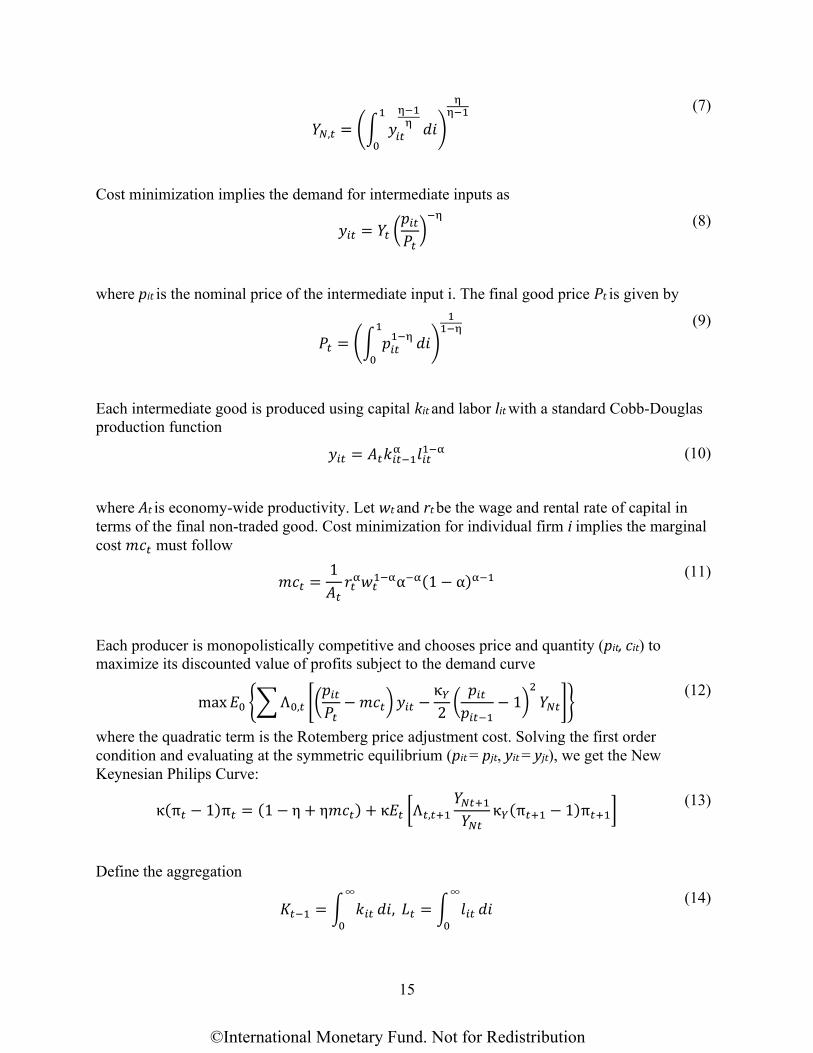
Non-traded Good A final non-traded good YN,t is produced from a continuum i ∈ [0,1] of intermediate inputs yit

under perfect competition. The production technology is given as:


15

𝑌𝑁,𝑡 = (∫ 𝑦𝑖𝑡

η−1η

1

0

𝑑𝑖)

ηη−1

(7)

Cost minimization implies the demand for intermediate inputs as

𝑦𝑖𝑡 = 𝑌𝑡 (𝑝𝑖𝑡

𝑃𝑡)

−η

(8)

where pit is the nominal price of the intermediate input i. The final good price Pt is given by

𝑃𝑡 = (∫ 𝑝𝑖𝑡1−η

1

0

𝑑𝑖)

11−η

(9)

Each intermediate good is produced using capital kit and labor lit with a standard Cobb-Douglas production function

𝑦𝑖𝑡 = 𝐴𝑡𝑘𝑖𝑡−1α 𝑙𝑖𝑡

1−α (10)

where At is economy-wide productivity. Let wt and rt be the wage and rental rate of capital in terms of the final non-traded good. Cost minimization for individual firm i implies the marginal cost 𝑚𝑐𝑡 must follow

𝑚𝑐𝑡 =1

𝐴𝑡𝑟𝑡

α𝑤𝑡1−αα−α(1 − α)α−1

(11)

Each producer is monopolistically competitive and chooses price and quantity (pit, cit) to maximize its discounted value of profits subject to the demand curve

max 𝐸0 {∑ Λ0,𝑡 [(𝑝𝑖𝑡

𝑃𝑡− 𝑚𝑐𝑡) 𝑦𝑖𝑡 −

κ𝑌

2(

𝑝𝑖𝑡

𝑝𝑖𝑡−1− 1)

2

𝑌𝑁𝑡]} (12)

where the quadratic term is the Rotemberg price adjustment cost. Solving the first order condition and evaluating at the symmetric equilibrium (pit = pjt, yit = yjt), we get the New Keynesian Philips Curve:

κ(π𝑡 − 1)π𝑡 = (1 − η + η𝑚𝑐𝑡) + κ𝐸𝑡 [Λ𝑡,𝑡+1

𝑌𝑁𝑡+1

𝑌𝑁𝑡κ𝑌(π𝑡+1 − 1)π𝑡+1]

(13)

Define the aggregation

𝐾𝑡−1 = ∫ 𝑘𝑖𝑡

∞

0

𝑑𝑖,  𝐿𝑡 = ∫ 𝑙𝑖𝑡

∞

0

𝑑𝑖 (14)


16

Since under the symmetric equilibrium we have kit = kjt and lit = ljt, we can simply aggregate the production function as

𝑌𝑁,𝑡 = 𝐴𝑡𝐾𝑡−1α 𝐿𝑡

1−α (15)

and the cost minimization of individual firms gives the relationship between the factor prices 𝑟𝑡

𝑤𝑡=

α

1 − α

𝐿𝑖𝑡

𝐾𝑡−1

(16)

Traded Good

The household receives endowments of the traded good when the non-traded good is produced. We assume the endowment is proportional to the amount of non-traded good produced, a simple reduced-form specification to capture the fact that production of the traded and non-traded goods are both correlated with the performance of the aggregate economy. Endowments are thus given by:

𝑌𝑇,𝑡 = χ𝑇𝑌𝑁,𝑡 (17)

The endowed traded good can be freely traded in the world open market. Each period, the household sells all its endowments to the world market, and then buys the traded good consumption bundle. The difference between the two is the net export of the home country.

1

𝑠𝑡𝐸𝑋𝑡 = 𝑌𝑇,𝑡 − 𝐶𝑇,𝑡

(18)

Capital Good The law of motion for the aggregate capital used by the intermediate good producers is:

𝐾𝑡 = (1 − δ)𝐾𝑡−1 + 𝐼𝑡 (19)

where δ is the capital depreciation rate, and It is the new capital investment. We assume

producing It amount of capital good incurs a total investment cost of (1 + Φ (𝐼𝑡

𝐼�̅�)) 𝐼𝑡 in terms of

non-traded good, where 𝐼�̅� is the steady state level of new capital investment. The particular

function form we use is Φ (𝐼𝑡

𝐼̅) =

κ𝐼

2(

𝐼𝑡

𝐼̅− 1)

2

.

The capital good producer produces It amount of capital using non-traded good and sells to the market at price 𝑄𝑡

𝐾 to maximize its profit:

max𝐼𝑡

𝑄𝑡𝐾𝐼𝑡 − (1 + Φ (

𝐼𝑡

𝐼 ̅)) 𝐼𝑡

(20)

Solving the first order condition gives the equilibrium price of capital:


17

𝑄𝑡𝐾 = 1 +

κ𝐼

2(

𝐼𝑡

𝐼 ̅− 1)

2

+ κ𝐼 (𝐼𝑡

𝐼 ̅− 1)

𝐼𝑡

𝐼 ̅

(21)

The total return for holding capital consists of two parts: collecting rents from firms using the capital and selling depreciated capital:

𝑅𝑡𝐾 = (1 − δ)𝑄𝑡

𝐾 + 𝑟𝑡 (22)

C. Banks

The setup of the banks follows Gertler and Karadi (2011). In each period, there is a unit measure of bankers. Each banker runs a bank. At the end of each period, each banker has a probability σ to continue in the next period as a banker and a probability 1 − σ of retiring. The retired bankers transfer all their net worth back to the household and are replaced by new bankers, who get start-up funds from the households. This retirement ensures bankers do not accumulate an infinite amount of wealth.

The role of bankers is crucial in this economy. As households do not directly invest in the firms, bankers channel funds from households as deposits and funding from foreign investors to make investments in the real economy. The objective of one individual banker in recursive form is:

𝑉(𝑛𝑗𝑡) = max 𝐸[Λ𝑡,𝑡+1((1 − σ)𝑛𝑡+1 + σ𝑉(𝑛𝑗,𝑡+1))] (23)

where njt is the banker j’s net worth, Λt,t+1 is the discount factor inherited from the representative household, and V (njt) is the value of the banker with net worth nt. In each period, bank j’s balance sheet is

𝑠𝑡𝑏𝑗𝑡∗ + 𝑏𝑗𝑡 + 𝑄𝑡

𝐾𝑘𝑗𝑡 = 𝑑𝑗𝑡 + 𝑠𝑡𝑑𝑗𝑡∗ + 𝑛𝑡 (24)

The liability side of the balance sheet includes 𝑑𝑗𝑡 and 𝑠𝑡𝑑𝑗𝑡

∗ . 𝑑𝑗𝑡 is the deposit from domestic households. 𝑠𝑡𝑑𝑗𝑡

∗ is home value of foreign funding 𝑑𝑗𝑡∗ denominated in the world currency. 𝑛𝑡 is

the banks’ net worth. The bank holds three types of assets: 𝑏𝑗𝑡 is home government bond, 𝑠𝑡𝑏𝑗𝑡∗

is the home value of foreign safe assets, and 𝑄𝑡

𝐾𝑘𝑗𝑡 is the value of capital. Aside from the balance sheet, banks face an additional financial constraint that limits their ability to raise funds, closely related to the participation constraint in Gertler and Karadi (2011). We frame the microfoundation of the constraint in the following moral hazard problem: in any period after receiving funds and buying assets, banks can either operate normally, or immediately liquidate their assets and take a fraction of the capital away for personal use. Investors would only supply funds to the banker if they believe the banker has no incentive to divert assets. We assume investors’ belief on the fraction of capital bank j can divert as:

γ(𝑥) = θ0 exp(−θ1𝑥) (25)


18

where 𝑥 =𝑠𝑡𝑏𝑗𝑡

∗

𝑛𝑡 is the relative amount of the foreign safe assets to net worth. The parameters θ0

and θ1 are both greater than 0. This setup resembles one in Aoki, Benigno and Kiyotaki (2018). It is one simple way to rationalize the empirical observation that banks around the world hold low-yield US treasury securities, even though domestic government bonds and capital may bring higher returns.

The participation constraint for bank j is then

𝑉(𝑛𝑡) ≥ γ (𝑠𝑡𝑏𝑗𝑡

∗

𝑛𝑡) (𝑄𝑡

𝐾𝑘𝑗𝑡) (26)

The left hand side is the value of operating normally, and the right hand side is the amount the banker can take away if diverting, from the perspective of investors’ belief. So, if the bank holds more foreign safe assets, it would have better credibility for investors who believe the banker can divert less assets, which relaxes the funding constraint for the bank, enabling it to raise more funds. Conditional on surviving, the banker’s net worth evolves as

𝑛𝑡+1 = 𝑅𝑡+1𝐾 𝑘𝑗𝑡 + 𝑅𝑡+1

𝐵 𝑏𝑗𝑡 + 𝑠𝑡𝑅𝑡+1𝐵∗ 𝑏𝑗𝑡

∗ − 𝑅𝑡+1𝑑𝑗𝑡 − 𝑠𝑡𝑅𝑡+1∗ 𝑑𝑗𝑡

∗ (27)

The banker’s budget constraint is the combination of its balance sheet and its net worth evolution. The banker’s optimization problem is to choose its asset and liability positions to maximize its value, under the balance sheet constraint (equation 24), the net worth evolution (equation 27) and the participation constraint (equation 26). Banker’s optimal choice Since in the banker’s balance sheet, net worth evolution and the participation constraint are all constant return to scale, it is straight forward to show that each banker’s value is 𝑉(𝑛𝑗𝑡) = ψ𝑡𝑛𝑗𝑡, so the objective function becomes

ψ𝑡 = 𝐸𝑡 [Λ𝑡,𝑡+1Λ(1 − σ + σψ𝑡+1ψ)𝑛𝑗𝑡+1

𝑛𝑗𝑡]

(28)

The participation constraint becomes

ψ𝑡 ≥ θ0 exp (−θ1

𝑠𝑡𝑏𝑗𝑡∗

𝑛𝑗𝑡)

𝑄𝑡𝐾𝑘𝑗𝑡

𝑛𝑗𝑡

(29)

Since we can scale all asset and liability positions by net worth n, the banker’s problem can be reduced to choose these positions as a fraction of net worth n. Thus, given that bankers are the same except how much net worth they originally have, all bankers choose the same fractions. Let the multiplier on the participation constraint be λt. Then it is straightforward to deduce the asset pricing equations from the first order conditions:

𝑅𝑡+1𝐵 = 𝑅𝑡+1 (30)

𝐸𝑡[Λ𝑡,𝑡+1(1 − σ + σψ𝑡+1) (𝑠𝑡+1

∗

𝑠𝑡𝑅𝑡+1

∗ − 𝑅𝑡+1) = 0 (31)


19

𝐸𝑡[Λ𝑡,𝑡+1(1 − σ + σψ𝑡+1)(𝑅𝑡+1𝐾 − 𝑅𝑡+1)] = λ𝑡θ0 exp (−θ1

𝑠𝑡𝐵𝑡∗

𝑁𝑡) 𝑄𝑡

𝐾 (32)

𝐸𝑡 [Λ𝑡,𝑡+1(1 − σ + σψ𝑡+1) (𝑠𝑡+1

𝑠𝑡𝑅𝑡+1

𝐵∗ − 𝑅𝑡+1)] = −λ𝑡θ0θ1 exp (−θ1

𝑠𝑡𝐵𝑡∗

𝑁𝑡)

𝑄𝑡𝐾𝐾𝑗𝑡

𝑁𝑡

(33)

Aggregation Summing up all banks’ balance sheets, we get the aggregate balance sheet of the whole banking sector:

𝑠𝑡𝐵𝑡∗ + 𝐵𝑡 + 𝑄𝑡

𝐾𝐾𝑡 = 𝐷𝑡 + 𝑠𝑡𝐷𝑡∗ + 𝑁𝑡 (34)

We assume the new banker gets a fraction ξ of the retiring bank’s capital holdings, so the aggregate banking sector’s net worth evolution is:

𝑁𝑡 = σ[𝑅𝑡𝐾𝐾𝑡−1 + 𝑅𝑡

∗𝐵𝑡−1 + 𝑠𝑡𝑅𝑡𝐵∗𝐵𝑡−1

∗ − 𝑅𝑡𝐷𝑡−1 − 𝑠𝑡−1𝑅𝑡𝐷𝑡−1∗ ] + ξ(𝑅𝑡

𝐾𝐾𝑡−1) (35) The objective function and the participation constraint can similarly be aggregated

ψ𝑡 = 𝐸𝑡 [Λ𝑡,𝑡+1(1 − σ + σψ𝑡+1)(𝑅𝑡+1𝐾 𝐾𝑡 + 𝑅𝑡+1

𝐵 𝐵𝑡 + 𝑠𝑡+1𝑅𝑡+1𝐵∗ 𝐵𝑡

∗ − 𝑅𝑡+1𝐷𝑡

− 𝑠𝑡𝑅𝑡+1𝐷𝑡∗)

1

𝑁𝑡]

(36)

ψ𝑡 ≥ θ0 exp (−θ1

𝑠𝑡𝐵𝑡∗

𝑁𝑡)

𝑄𝑡𝐾𝐾𝑗𝑡

𝑁𝑡

(37)

D. Foreign Investor

We model the foreign investments into the home country as a single representative risk-neutral foreign investor supplying foreign credit to the domestic banking sector. This is a simplifying assumption that enables analyzing the effect of capital flow shocks easily. The risk neutral foreign investor has problem:

max𝐷∗

𝐸 [(𝑅𝑡∗ − 𝑅𝑡

𝐵∗)𝐷𝑡∗] −

1

2χ𝑑,𝑡

(𝐷𝑡∗)2

(38)

Here we assume foreign funding incurs a quadratic cost 1

2χ𝑑,𝑡(𝐷𝑡

∗)2 to the foreign investors,

depending on the amount of credit extended to the home banking sector. The solution to the problem gives the foreign credit supply function:

𝐷𝑡∗ = χ𝑑,𝑡(𝑅𝑡

∗ − 𝑅𝑡𝐵∗) (39)

We observe that the amount of foreign credit supply depends on two quantities: the expected excess return over foreign interest rate (𝐸 [

𝑠𝑡

𝑠𝑡+1] 𝑅𝑡 − 𝑅𝐵∗) and the cost parameter χd,t. We use

these two quantities to capture two kinds of capital flows. The first is the passive capital flow generated by a shock on the foreign interest rate. Capital inflows to emerging markets due to a relative decline in the U.S. policy rate falls in this category. The second is the active capital flow


20

generated by a shock on the parameter χd,t. This can capture capital flow fluctuations without a change in the interest rate, which can include “hot money” inflows and speculation.

E. Government For simplification, the government in this model is a combination of the fiscal and monetary authorities and deploys only rule-based policies. It conducts three types of policies: monetary policy, fiscal policy and foreign exchange intervention policy. The government’s budget constraint is:

𝑠𝑡𝐹𝑡 = 𝑅𝑡𝐵∗𝑠𝑡𝐹𝑡−1 + 𝐵𝑡 − 𝑅𝑡𝐵𝑡−1 + 𝑇𝑡 (40)

where Ft is the government’s reserve holding, which is in the foreign safe asset with a return 𝑅𝑡𝐵∗.

Bt is the domestic bond issued by the government, which has domestic return Rt. Since the return of the domestic bond is higher than that of foreign reserves, the government charges a tax so its debt position would not explode. Monetary Policy We consider the government follows a simple standard Taylor rule.

it = i̅ + ρπ(πt − π̅) + ρy(YN,t − YN,t̅̅ ̅̅ ̅) (41)

Fiscal Policy In the model, as fiscal policy is not of our primary interest, we assume the function of fiscal policy is to finance the government budget by implementing a lump-sum tax, as:

𝑇𝑡 = ρ𝑇(𝐵𝑡−1 − �̅�) (42) Foreign Exchange Intervention We are interested in rule-based sterilized FX intervention. In the baseline specification, we assume no intervention, so

Ft = �̅� The sterilized FX intervention is specified as

𝐹𝑡 = �̅� + ρ𝐹𝑆(𝑠𝑡 − �̅�) + ρ𝐹𝐷(𝐷𝑡∗ − 𝐷∗̅̅̅̅ ) (43)

The amount of reserves the government wishes to hold depends on both exchange rate movements and capital flow fluctuations. Choosing a reserve amount Ft is automatically sterilized because the government budget constraint must hold and the tax Tt only responds to the previous time period Bt−1, so the government must change the corresponding amount in Bt.

F. Market Equilibrium Non-traded output is either consumed or invested in the capital good production

𝑌𝑁,𝑡 = 𝐶𝑁,𝑡 + 𝐼𝑡 +κ𝐼

2(

𝐼𝑡

𝐼 ̅− 1)

2

𝐼𝑡 +κ

2(π𝑡 − 1)2𝑌𝑁,𝑡

(44)

Traded endowment is either consumed or exported

𝑌𝑇̅̅ ̅ = 𝐶𝑇,𝑡 +

1

𝑠𝑡𝐸𝑋𝑡

(45)


21

The balance of payments must clear

𝐹𝑡 + 𝐵𝑡∗ − 𝐷𝑡

∗ = 𝑅𝑡𝐵∗𝐹𝑡−1 + 𝑅𝑡

∗𝐵𝑡−1∗ − 𝑅𝑡

∗𝐷𝑡−1∗ +

1

𝑠𝑡𝐸𝑋𝑡

(46)

The exogenous shocks of the model are the productivity shock At, the foreign interest rate shock 𝑅𝑡

𝐵∗ and the capital flow shock χDt . The competitive equilibrium of the model is given by a set of sequences of allocations 𝐶𝑁,𝑡, 𝐶𝑇,𝑡, 𝐿𝑡, 𝐷𝑡, 𝐸𝑋𝑡, 𝑇𝑡, 𝑌𝑇,𝑡, 𝐻𝑡 , 𝑚𝑐𝑡, 𝑌𝑁,𝑡, 𝐼𝑡 , 𝑁𝑡, 𝐵𝑡, 𝐵𝑡

∗, 𝐷𝑡∗, 𝐾𝑡, 𝐹𝑡 (17

variables), prices 𝑠𝑡, 𝑤𝑡, π𝑡 , 𝑖𝑡, 𝑅𝑡, 𝑅𝑡∗, 𝑄𝑡

𝐾, 𝑅𝑡𝐾, 𝑅𝑡

𝐵, 𝑟𝑡 (10 variables), auxiliary variables Λ𝑡,𝑡+1, ψ𝑡, and multiplier λt satisfying equations (1) to (46). The household budget constraint is automatically satisfied given the resource constraints and budget constraints from the other agents. Annex IV presents a schematic overview of the model.

IV. CALIBRATION Table AV.1 lists the parameter values used in our calibration exercise. We normalize the steady-state total output to 1 in the model, so other quantity variables are expressed in fractions of GDP. Table AV.2 lists the non-stochastic steady state level of variables in the model. We use an Asian EM average as a benchmark for our baseline calibration, for which we use data from the post-crisis low interest rate period (2009 to 2018) because this period is our primary focus. 9 The frequency of the model is quarterly. The parameters of the household are mostly standard in the literature. We set the parameters of the banking sector (σ, ξ, θ0, θ1) such that they match the average interest rate differential and the banking sector gross FX assets and liabilities in our EM Asia dataset. For simplicity, the outside world is normalized to have zero inflation and real exchange rate 1 in the steady state. We use the US 3-month T-bill rates as the foreign interest rate, which includes the convenience premium of holding safe US treasuries. As a common case of multiplicity of steady state in small open economy models, in our model each level of steady state FX reserves is associated with one different steady state. We pin it down by choosing the steady state FX reserves level as 1.5 times GDP as the ten-year average for EM Asia data, which is also large enough for implementing FX intervention under the size of shock observed in the data. We also calibrate the size of FX intervention such that they match the volatility of change of FX reserves in the data (8.9 percent of GDP).

A. Capital Flow Shock Figure AV.1 shows the impulse responses to a temporary capital outflow shock with and without FXI. Because the primitive capital flow shock variable χ is not directly observable in the data, we choose the size of one standard deviation of the shock such that it leads to one standard deviation of banks’ gross external assets over GDP observed in the data. The responses of all the variables are proportional to their steady state values.

9 We use Indonesia, Malaysia, Philippines, and Thailand.


22

In the figure, the solid blue line shows the response of different macroeconomic variables to the capital outflow shock without any policy intervention. The shock to foreign investors lowers the foreign credit supply function (equation 39), leading them to take FX funding out of the home economy. This tightens bank balance sheets and net worth (equations 34 and 35), leading to a 27 percent drop in bank external borrowing and a 29 percent drop in bank external assets relative to their steady state levels. The involuntary decline in the bank’s external balance sheet leads to a significant financial tightening via the asset side, with liquidity value falling by 52 percent, forcing banks to cut investment to the real sector by 7.4 percent. As a result, output falls by 0.6 percent. All sides of the real sector are affected. Labor, wages, the price of capital and marginal cost all significantly drop, leading to deflation. A central bank conducting a conventional monetary policy now lowers the interest rate to stimulate the economy, though this is not enough to restore output. The observed exchange rate dynamics are in contrast to the conventional risk sharing mechanism predicted in Backus and Smith (1993), where a fall in output should lead to an appreciation of the exchange rate, serving as a shock absorber to offset the drop on consumption. In the model simulation, the real exchange rate depreciated by 2.2 percent, further hurting the welfare of the representative consumer. The red dashed line is the response if the central bank reacts to the capital outflow shock with FX intervention. Here, according to the intervention rule (equation 43), the central bank should sell reserves to support the domestic financial sector. Accordingly, the central bank sells 8.9 percent of FX reserves to the economy, which greatly improves the gross external position of banks by substituting out banks’ foreign borrowing with the FX injection. Therefore, although gross FX liability falls further than without policy intervention, gross FX assets decline only by half. Financial conditions are no longer as tight and the resulting decline in investment and output is lower. In general, we argue that sterilized FXI is an effective policy tool targeting exchange rate depreciation caused by shocks to the financial sector, as experienced by many Asian emerging markets. These countries share a similar structure of financial markets: large FX positions together with financial systems which are generally less developed, with limited hedging opportunities, while being highly integrated into international financial markets. Consistent with practical insight from policy makers in Asia, we show that FXI can stabilize the domestic financial system when faced with a large external capital outflow shock.

B. Productivity Shock Figure AV.2 shows the impulse responses with and without FXI to a TFP shock of size 1 percent. Output falls by 0.96 percent, with investment and labor and output all falling. Though both the productivity and the capital outflow shocks lead to a recession, the mechanism that drives the recession is vastly different. Under TFP shock, the conventional risk sharing channel dominates. The response of the financial sector is quite small compared to the case with capital outflow shock. Bank gross FX assets fall only by 5 percent, which is about 1.8 percent of GDP. Gross FX liabilities fall only by 3 percent.


23

Without a large financial channel, the exchange rate indeed appreciates, serving as a shock absorber as in conventional wisdom. Although the productivity shock affects the value of equities banks hold, thereby tightening their financing constraint, given the size and structure of balance sheets, a productivity shock does not yield the same exchange rate dynamics as in the direct funding shock discussed above. In this case, we arrive at the same conclusion to that of conventional wisdom: FXI is not effective where the exchange rate is a shock absorber. We see here if the central bank wants to stabilize the exchange rate, it needs to buy reserves from the market to offset the appreciation. If its primary target is to stabilize the exchange rate, then the central bank could be seen as successful. However, buying reserves during a recession would certainly worsen the economy. In the figure, we can clearly see that with FXI the output response is lower than without FXI. This constitutes our second argument: FXI can be costly when the exchange rate is indeed a shock absorber. Implementing FXI in this case switches off the risk sharing channel, which invalidates the primary role of the exchange rate in the financial market. This would suggest that the decision whether to deploy FXI should depend on the nature of shock that the economy is facing. It is important to underscore the key role the structural characteristics of bank balance sheets in Asian EMs play in driving these results. Banks have high FX exposures on their balance sheets, and financial markets are generally less developed, limiting the availability of FX hedging in the broader economy, making the effect of the exchange rate on balance sheets nontrivial. Both the financial and real shocks affect bank’s net worth through the value of equities banks hold. However, with high FX assets and liabilities positions, the calibration of the model is such that under a real shock, the exchange rate still works as a shock absorber, while for the financial shock, the exchange rate depreciates to directly tighten banks’ financing constraints. Indeed with a different structure of bank balance sheets, we would get varying results.

V. ALTERNATIVE POLICIES

Although FXI is the most widely used measure in responding to external shocks for Asian emerging markets, it is certainly not the only one (IMF 2019a). Other measures commonly deployed include macroprudential policies (MPM), capital flow measures (CFMs), and augmented monetary policy targeting external conditions. Indeed, these policies are not mutually exclusive and may not share the same primary goal. In this section, we focus on the question of how these policies compare when reacting to external financial shocks.

A. Capital Flow Measures (CFMs)

CFMs are generally used in a limited context and in extraordinary times. There are many distinct types of CFM, and the specific CFM we consider in this model is a tax on foreign funding, which corresponds to tax on portfolio inflows in real-world implementation. Here the foreign investor’s maximization of her after-tax expected return gives the credit supply function,

𝑑𝑡∗ = 𝜒𝑑,𝑡 ((1 − 𝜏𝑑,𝑡)𝑅𝑡

∗ − 𝑅𝑡𝐵∗)


24

where 𝜏𝑑,𝑡 is the tax rate on foreign investment in domestic banks. We consider the following rule-based CFM:

𝜏𝑑,𝑡 = 𝜌{𝜏𝑠}(𝑠𝑡 − �̅�) + 𝜌{𝜏𝑑}(𝐷𝑡∗ − 𝐷∗̅̅̅̅ )

Under such a rule, the government imposes a higher tax when the exchange rate is appreciating and/or with larger FX liabilities and a lower tax when the exchange rate is depreciating and/or with lower FX liabilities.

B. Augmented Monetary Policy

Empirical studies have shown that monetary policy in Asian emerging markets not only considers standard objectives (inflation and output gap), but also additional unconventional considerations such as the global financial cycle. In the model, we consider the following augmented Taylor rule:

𝑖𝑡 = 𝑖̅ + 𝜌𝜋(𝜋𝑡 − �̅�) + 𝜌𝑦(𝑌{𝑁𝑡} − {𝑌𝑁}̅̅ ̅̅ ̅̅ ) + 𝜌𝑖𝑑(𝐷𝑡∗ − 𝐷∗̅̅̅̅ ) + 𝜌𝑖𝑠(𝑠𝑡 − �̅�)

Under such a rule, the central bank raises the interest rate following a depreciation and with lower FX liabilities, and lowers the interest rate following an appreciation and with greater FX liabilities.

C. Macroprudential Measures

MPMs are the widely used among Asian EMEs and can take several forms. Among the different types of MPMs, reserve requirement (RR) is mostly used in Asian emerging markets (IMF 2019c). In the model, we consider the MPM to be the reserve requirement on FX borrowing of banks. Now the bank balance sheet becomes:

𝐵𝑡 + 𝑠𝑡𝐵𝑡∗ + 𝑄𝑡

𝐾𝐾𝑡 = 𝐷𝑡 + 𝑠𝑡(1 − 𝜏𝑚,𝑡 )𝐷𝑡∗ + 𝑁𝑡

where 𝜏𝑚,𝑡𝐷𝑡∗ is the amount of reserve that the bank must deposit at the central bank. We assume

the bank reserves earn the same return as the FX reserves held by central bank. So banks’ evolution of net worth becomes

𝑁𝑡 = 𝜎[𝑅𝑡𝐾𝐾𝑡−1 + 𝑅𝑡𝐵𝑡−1 + 𝑠𝑡𝑅𝑡

𝐵∗𝐵𝑡−1∗ + 𝑠𝑡𝜏𝑚,𝑡−1𝑅𝑡

𝐵∗𝐷𝑡−1∗ − 𝑅𝑡𝐵𝐷𝑡−1 − 𝑠𝑡𝑅𝑡

𝐵∗𝐷𝑡−1∗ ]

The government budget constraint now becomes

𝑠𝑡𝐹𝑡 = 𝑅𝑡𝐵∗𝑠𝑡𝐹𝑡−1 + 𝐵𝑡 − 𝑅𝑡𝐵𝑡−1 + 𝑠𝑡𝜏𝑚,𝑡𝐷𝑡

∗ − 𝑅𝑡𝐵∗𝑠𝑡𝜏𝑚,𝑡−1𝐷𝑡−1

∗ + 𝑇𝑡

From the government budget constraint, it seems that changing the value of 𝜏𝑚,𝑡 could have the same effect of changing the value of F̅t in the case of FXI. However, they are different because changing 𝜏𝑚,𝑡 also changes the asset pricing equation for the banks through 𝑁𝑡. We consider the following rule-based policy for reserve requirements:


25

𝜏𝑚,𝑡 = 𝜌𝑚𝑠(𝑠𝑡 − �̅�) + 𝜌𝑚𝑑(𝐷𝑡∗ − 𝐷∗̅̅̅̅ )

Here, the government imposes higher reserve requirements when the exchange rate appreciates and with larger FX liabilities and lower reserve requirements when the exchange rate depreciates and with lower FX liabilities.

D. Comparison Across Policies

To compare the alternative policies, we use our calibration from Section IV as a benchmark. Our exercise shows that all alternative policies are effective in smoothing the recession caused by a capital outflow shock. For each of the alternative policies, we calibrate the parameters of the policies to match the output response of our baseline FXI case. Our objective is to compare the response of other variables for these policies under the capital outflow shock. Table AV.3 summarizes our result. We first compare FXI with MPM. The responses are quite similar because they both target the relationship between the banking sector and foreign investors. The only difference is that MPM distorts domestic banks’ demand for foreign funds via their marginal propensity to receive FX borrowing. Under a reduction of the reserve requirement, banks are willing to incur more FX borrowing. Since borrowing is more costly than getting funding from central bank reserves, there is a consumption loss compared to FXI. Our computation shows that the difference is at most moderate. CFM, on the other hand is a distortion on the foreign investor, affecting the supply of foreign funding. Reducing the tax on the foreign investors is essentially a subsidy to them, shifting the foreign funding supply function to the right. Thus, we observe a drop in foreign borrowing amounting to about half of that in the FXI case. The subsidy must come from consumer welfare, and therefore there is a cost to consumption. Augmented monetary policy has some distinct features when compared to the other policies, because the mechanism of monetary policy is fundamentally different. Unlike other policies that directly interfere with banks’ reaction functions, using monetary policy can stimulate the economy to offset the loss caused by the financial sector. In our case, augmented monetary policy drives inflation up, causing households to work more under sticky prices. This stimulus then spills over to the banks. Naturally, this policy would experience similar side effects from economic stimulus. Here, the increase in labor hours is a direct cost to welfare. In summary, we argue that in some cases FXI may be a preferred policy response under capital outflow shocks. This is because FXI purely targets capital flows without creating additional distortions as compared to alternative policies, which affect banks’ propensity to borrow. In practice, however, we rarely observe an economy being subject a single, identifiable shock. Other policies, or coordination of multiple policies may be optimal if the distortion they create is able to offset other shocks or frictions. We also do not consider other costs to the use of FXI; for inflation targeters, consistent use of FXI could distort signaling about the monetary policy framework and compromise the credibility of the central bank, unanchoring inflation expectations, and there may be costs from persistent sterilization on financial market development. This would be a fruitful avenue for further research.


26

E. Optimal Policy

We suppose the central bank faces a policy objective of minimizing the following loss function:

𝐿 = min 𝐸 [𝑦𝑡′𝑊𝑦𝑡]

where y includes a vector of variables that are the central banks’ target deviated from the steady state, and W is the weighting matrix. As in our framework, the central bank implements two policies: monetary policy to set the domestic interest rate, and one of setting the exchange rate in response to external shocks. We assume that the central bank uses monetary policy solely for domestic conditions and implement exchange rate policy in response to external shocks. Thus, we face a two-stage problem of finding the respective optimal policies. We first consider monetary policy. We assume the central bank targets the inflation and output when setting the domestic interest rate. We set external shocks to zero and leave only the productivity shocks. This gives the optimal monetary policy parameters ρy = 0.08 and ρπ = 1.2. Next, we consider each of the exchange rate policies. We study the optimal exchange rate policy in two settings, of which one is the more realistic case with both shocks, and the others are the hypothetical case where there is only an external shock or only a productivity shock. We include the hypothetical cases to highlight the trade-offs of implementing exchange rate policy. Specifically, we let the government’s objectives be output, inflation and the exchange rate 𝑦 ={𝑌, π, 𝑠}. This simple specification captures the idea that the government’s policy stance toward external conditions is to target output, internal stability and external stability. In reality the government would certainly have a broader range of targets. This specification nevertheless captures the most important categories of government objectives.

Table 2: Comparison of Loss Function Loadings by Type of Shock FXI CFM MPM Augmented MP

Shocks Both D* A Both D* A Both D* A Both D* A Loading

on D* 0.938 0.96 0.879 0.24 0.09 0.24 0.06 -0.04 -1.20 0.09 0.036 0.049

Loading on S

-10.1 27 -12.7 0.8 -0.06 1.17 -2.01 -3.84 -0.25 0.78 -0.68 1.28

Loss 0.007 9.0e-06 0.007 0.017 0.001 0.016 0.040 0.018 0.022 0.009 0.001 0.006 Note: Three types of shocks are considered: productivity shocks (A), capital flow shocks (D*) and both productivity and capital flow shocks simultaneously (“Both”).

The table above compares the parameters and loss functions for alternative policies under different shocks: both shocks (productivity (A) and capital flows (D*)) and the individual, independent shocks (A and D*). The results are broadly consistent with insights given in the previous sections.


27

First, we see FXI works well when the economy faces only an external shock (D*). The loss function gives a value very close to 0, implying that FXI can nearly fully stabilize the economy to external volatility. The loss for CFM and MPM cases are significantly higher because they react to the external shock by introducing additional distortions (the marginal cost of capital) that increases the overall loss. Second, we see that FXI is not as effective under a productivity shock as compared to an external shock, yielding a much higher loss. The loading on the exchange rate sign is the opposite, consistent with our insight in the previous section that under a productivity shock, applying the same FXI as under external shock would make the economy even worse. The other policies also show a similar pattern, further suggesting any effort to stabilize the exchange rate can be counterproductive when the exchange rate is indeed a shock absorber. For the more realistic case of both shocks occurring, we see that FXI alone is not sufficient as it cannot eliminate the losses caused by the productivity shock. Policies that bring extra distortions (CFMs and MPMs) perform even worse. Indeed in practice, not only may shocks occur simultaneously, but it is difficult for policymakers to identify which type of shock they are facing. This illustrative exercise highlights that in there are indeed limits to the reach of FXI, and complementary policies must be used to address the myriad shocks EMs are exposed to.

VI. CONCLUSION

Emerging market economies are increasingly integrated with the global economy and the international financial cycle, including through large and volatile capital flows, which play a defining role in economic fluctuations. This paper has highlighted the important role banks (and financial intermediaries more broadly) can play in transmitting external shocks to the real economy in such countries. Banking systems with large FX exposures on both sides of their balance sheets, as in emerging Asia, can serve as a key shock propagation mechanism. We show that adverse external financial shocks, such as capital outflows, can directly affect banks’ funding with an exchange rate depreciation tightening their financing constraints, causing a contraction in credit extended by banks, which leads to a decline in investment and output. Under such shocks, the exchange rate acts as a shock amplifier rather than a shock absorber. By contrast, the impact of adverse nonfinancial shocks, such as productivity or terms of trade shocks, is generally less severe given bank balance sheets are not directly affected; here the exchange rate behaves more conventionally as a shock absorber. This paper has also examined policy options available to such economies to mitigate the macrofinancial impact of external shocks. We argue that FXI can play an important role in mitigating external financial shocks by providing FX funding during times of stress and dampening the effect of exchange rate fluctuations on bank balance sheets. However, it is important to stress that FXI is no silver bullet. In the case of nonfinancial shocks, where the exchange rate continues to act as a shock absorber, a standard Taylor rule improves welfare. We also abstract more generally from the potential longer-term costs to FXI, such as to central bank credibility and financial market development, which are key considerations. Similarly, there is also some role for cyclical macroprudential policies (a reserve requirement on foreign bank liabilities) and CFMs (cyclical tax on foreign borrowing) in managing external shocks. Such measures can help stabilize the bank balance sheet and external exposures respectively, allowing


28

room for policy interest rate to focus on the more traditional macro stability objective, and leading to welfare gains. This would support the assignment of traditional monetary policy interest rate for price and output, and macroprudential policy for financial stability risks. However, such policies can induce welfare losses due their distortionary effects on banks’ propensity to borrow. Ultimately, the optimal policy response to external shocks depends heavily on the characteristics of the economy together with the types of shocks it faces, which may be difficult to identify in practice. The operational costs of alternative policies must also be weighed.


29

ANNEX I. SUMMARY STATISTICS

Table AI.1. Monthly Frequency

Table AI.2. Quarterly Frequency

Country Mean St. Dev Freq Mean St. Dev Freq Mean St. Dev Freq Mean St. Dev Freq Mean St. Dev FreqEmerging 1.15 10.99 1254 0.85 5.58 1254 0.15 1.33 1308 0.94 2.09 1254 0.62 6.30 1308Advanced 1.09 5.90 716 0.64 3.31 716 0.04 2.07 872 0.51 3.00 716 0.44 7.53 435

AUS 1.46 6.17 210 1.02 3.31 210 0.11 2.09 218 0.89 3.42 210CHN 0.95 3.66 169 0.91 5.26 169 0.11 1.20 218 1.16 1.40 169 1.10 7.13 218IDN 0.66 9.21 218 0.95 6.23 218 0.16 2.13 218 1.20 2.50 218 0.54 5.40 218IND 2.79 22.06 218 0.46 5.38 218 0.51 0.66 218 1.04 2.44 218 0.61 5.67 218JPN 0.47 2.71 215 0.42 3.29 215 -0.13 2.24 218 0.15 2.62 215 0.35 8.31 217KOR 0.95 4.00 206 0.69 3.31 206 0.02 1.89 218 0.64 2.83 206 0.53 6.69 218MSY 1.07 7.98 218 1.25 5.19 218 -0.08 1.20 218 0.62 1.92 218 0.40 4.85 218NZL 2.11 11.90 85 0.19 3.32 85 0.15 2.04 218 0.18 3.09 85PHL 0.80 5.03 213 0.84 6.03 213 0.10 1.29 218 0.87 2.15 213 0.40 6.40 218THA 0.60 4.86 218 0.69 5.28 218 0.11 1.03 218 0.78 1.77 218 0.65 7.87 218

Note: All variables are expressed in m/m growth, with the broadest coverage from 2001M12-2020M2

Foreign assets Foreign liabilities REER Credit to private sector IIP

Country Mean St. Dev Freq Mean St. Dev Freq Mean St. Dev Freq Mean St. Dev Freq Mean St. Dev FreqEmerging 3.05 17.11 414 2.59 9.77 414 0.27 2.48 438 2.87 3.96 414 1.82 3.15 428Advanced 3.15 10.20 240 2.08 6.86 240 0.13 3.79 291 1.68 5.44 240 0.70 2.20 284

AUS 4.29 9.36 70 3.08 5.95 70 0.40 3.84 73 2.70 6.36 70 0.96 2.16 71CHN 2.87 6.76 55 3.13 11.46 55 0.32 2.24 73 3.45 3.06 55 2.52 2.19 71IDN 1.80 15.93 72 2.73 9.10 72 0.38 3.54 73 3.72 4.49 72 1.70 2.12 71IND 6.28 32.98 72 1.64 11.54 72 0.33 2.63 73 3.18 4.42 72 2.30 3.21 71JPN 1.50 5.75 71 1.49 8.45 71 -0.43 4.21 73 0.50 5.31 71 0.02 1.56 71KOR 2.71 6.92 72 2.23 6.43 72 0.10 3.51 73 2.21 4.49 72 0.75 2.06 71MSY 3.07 12.80 72 3.68 8.22 72 -0.22 2.02 73 1.92 3.46 72 1.31 2.68 71NZL 5.68 22.04 27 0.60 5.17 27 0.45 3.57 72 0.70 4.98 27 1.06 2.74 71PHL 2.27 7.13 71 2.38 8.82 71 0.35 2.30 73 2.66 4.49 71 1.94 4.01 71THA 1.96 9.88 72 2.11 9.61 72 0.44 1.81 73 2.45 3.18 72 1.17 3.96 73

Note: All variables are expressed in q/q growth, with the broadest coverage from 2001Q4-2019Q4

Foreign assets Foreign liabilities REER Credit to private sector Investment


30

ANNEX II: PANEL VAR ESTIMATES

Notes: A quarterly panel VAR is estimated by GMM. Reported numbers show the coefficients of regressing the column variables on the row variables. Coefficients and p-values are reported. Endogenous variables are g_fl: growth in foreign liabilities, g_fa: growth in foreign assets, g_reer: change in the real effective exchange rate, positive values are an appreciation; g_credit: growth in credit to the private sector, and g_inv: growth in real investment (GFCF). All growth rates are computed quarter on quarter. Exogenous variables are inflation: CPI inflation; g_us: US growth; g_tot: change in the terms of trade index, and an external financing shock (the exogenous monetary policy shock e_mp shown in this table; excess bond premium, the VIX, and the US federal funds rate are used as alternative measures). L and L2 are the first and second period lags, respectively.

(1) (2) (3) (4) (5) (1) (2) (3) (4) (5) (1) (2) (3) (4) (5)VARIABLES g_reer g_fl g_fa g_credit g_inv g_reer g_fl g_fa g_credit g_inv g_reer g_fl g_fa g_credit g_inv

L.g_reer 0.0842* -0.122 0.306 -0.0118 -0.0532 0.127** -0.197 0.301 -0.0483 -0.0112 -0.113 -0.193 -0.0452 0.0237 -0.104*-0.0843 -0.458 -0.309 -0.908 -0.34 -0.0424 -0.407 -0.54 -0.714 -0.909 -0.259 -0.408 -0.879 -0.904 -0.0885

L2.g_reer -0.0715 0.0787 -0.101 -0.1 -0.0136 -0.108 0.318 -0.181 -0.0743 0.0279 -0.0051 0.0363 -0.0683 -0.0114 -0.0721*-0.309 -0.583 -0.708 -0.326 -0.735 -0.122 -0.163 -0.722 -0.49 -0.702 -0.965 -0.821 -0.676 -0.935 -0.0553

L.g_fl -0.0299** 0.0311 0.0538 -0.0188 -0.000404 -0.0203 0.0488 0.0203 -0.027 0.0105 -0.0911 -0.105 -0.0514 0.0329 -0.0215-0.0387 -0.595 -0.499 -0.422 -0.979 -0.115 -0.484 -0.836 -0.264 -0.545 -0.144 -0.352 -0.668 -0.709 -0.432

L2.g_fl -0.0148 0.105** 0.130* -0.00708 -0.0332*** 0.00132 0.127** 0.125* 0.0101 -0.0310** -0.158*** -0.177 -0.177 -0.148 -0.0518***-0.237 -0.0383 -0.0578 -0.715 -0.00666 -0.927 -0.0305 -0.0906 -0.613 -0.0352 -0.00723 -0.204 -0.157 -0.11 -0.00909

L.g_fa 0.00451 -0.0363 -0.11 0.00828 0.0128 0.0144* -0.0409 -0.145* 0.0138 0.0109 -0.0422 -0.0147 0.149 -0.0478 0.00607-0.611 -0.158 -0.143 -0.624 -0.266 -0.0767 -0.138 -0.0569 -0.436 -0.372 -0.382 -0.86 -0.189 -0.505 -0.817

L2.g_fa 0.0169* 0.00309 0.0349 0.00875 -0.00659 0.0195** -0.00696 0.00985 0.00591 -0.00808 0.0823 0.275*** 0.376*** 0.131 0.0133-0.0512 -0.914 -0.672 -0.627 -0.418 -0.0253 -0.818 -0.911 -0.755 -0.352 -0.135 -0.0079 -0.000334 -0.154 -0.56

L.g_credit 0.255*** 0.197* -0.381* 0.0429 0.0721** 0.167*** 0.19 -0.708** 0.0523 0.117** 0.475*** 0.393** 0.0473 0.0615 0.0667**-9.09E-10 -0.0914 -0.0537 -0.496 -0.0194 -0.0000753 -0.238 -0.0168 -0.499 -0.013 -3.72E-08 -0.0137 -0.799 -0.627 -0.0391

L2.g_credit -0.0355 0.00815 -0.218 0.0544 0.0922** 0.0127 -0.164 -0.363 0.0629 0.0341 0.0275 0.208 0.0284 0.0411 0.173***-0.358 -0.951 -0.373 -0.384 -0.0107 -0.781 -0.398 -0.332 -0.407 -0.476 -0.71 -0.123 -0.879 -0.735 -0.000313

L.g_inv -0.0599 0.166 -0.542* 0.126 -0.095 -0.0311 0.191 -0.558 0.126 -0.126 -0.0699 0.0938 0.23 0.137 0.0123-0.207 -0.319 -0.0619 -0.14 -0.165 -0.499 -0.336 -0.116 -0.199 -0.13 -0.622 -0.701 -0.536 -0.544 -0.87

L2.g_inv -0.00116 0.106 0.109 0.091 0.0402 0.0279 0.239 0.143 0.165** 0.0424 -0.184 -0.490* -0.015 -0.252 0.0402-0.979 -0.442 -0.708 -0.195 -0.499 -0.47 -0.133 -0.682 -0.0236 -0.541 -0.257 -0.0754 -0.965 -0.305 -0.662

e_mp 0.0516 -1.588* 0.195 -1.510*** -0.365* 0.338 -1.855** 0.88 -1.163** -0.302 -0.354 -1.103 -0.997 -1.885* -0.498**-0.891 -0.0582 -0.889 -0.00159 -0.0988 -0.212 -0.0383 -0.675 -0.0114 -0.359 -0.669 -0.454 -0.425 -0.0664 -0.011

g_tot 0.0213 0.117 0.121 0.0920** 0.0282 0.0089 0.0955 0.0993 0.125*** 0.0275 0.132 0.282 0.307 -0.06 0.0374-0.513 -0.156 -0.29 -0.0347 -0.256 -0.722 -0.201 -0.438 -0.00121 -0.328 -0.34 -0.294 -0.131 -0.757 -0.287

g_us 0.345 0.826 1.73 0.551 0.865*** 0.441 1.985 1.939 0.868 1.104** 0.106 -0.713 1.509 -0.127 0.485*-0.285 -0.376 -0.254 -0.258 -0.00424 -0.185 -0.12 -0.388 -0.105 -0.0173 -0.863 -0.524 -0.241 -0.89 -0.0981

inf 0.00815 0.151 0.177 0.332** -0.0346 0.0515 0.0766 0.206 0.327** -0.0753 -0.213 1.520** 0.678 0.558 0.161-0.947 -0.611 -0.731 -0.0247 -0.708 -0.682 -0.819 -0.722 -0.0389 -0.464 -0.523 -0.0139 -0.341 -0.337 -0.373

Observations 487 487 487 487 487 308 308 308 308 308 179 179 179 179 179pval in parentheses *** p<0.01, ** p<0.05, * p<0.1

Full Sample Emerging Economies Advanced Economies


31

ANNEX III. PANEL VAR IMPULSE RESPONSE FUNCTIONS

Figure AIII.1. Monthly Frequency

A. Specification with IIP (a) External financial shock (VIX)

(b) Foreign assets

(c) Foreign liabilities

(d) Real exchange rate appreciation

Note: This panel shows cumulative orthogonalized impulse response functions depicting the impact over 10 quarters of the following shocks: (a) a tightening in external financial conditions (VIX); and an increase in (b) foreign assets, (c) foreign liabilities, and (d) the real exchange rate, on foreign assets, foreign liabilities, the real exchange rate, credit growth and the index of industrial production (IIP) respectively. IRFs are estimated at a monthly frequency for the full sample (blue lines), EMs (red lines) and AEs (black line). All shocks are of one standard deviation size.


32

B. Specification without IIP

(a) External financial shock (VIX)

(b) Foreign assets


(d) Real exchange rate appreciation

Note: This panel shows cumulative orthogonalized impulse response functions depicting the impact over 10 quarters of the following shocks: (a) a tightening in external financial conditions (VIX); and an increase in (b) foreign assets, (c) foreign liabilities, and (d) the real exchange rate, on foreign assets, foreign liabilities, the real exchange rate, and credit growth respectively. IRFs are estimated at a monthly frequency for the full sample (blue lines), EMs (red lines) and AEs (black line). All shocks are of one standard deviation size.


33

Figure AIII.2. Quarterly Frequency

A. Alternative external shocks (i) increase in VIX (tightening of external financial conditions)

(ii) increase in terms of trade

B. Alternate specification including corporate debt (a) External financial shock

(a) External financial shock

Notes: A: This panel shows cumulative orthogonalized impulse response functions depicting the impact over 10 quarters of an increase in (a) the VIX and (b) the terms of trade on foreign assets, foreign liabilities, the real exchange rate, credit growth and investment respectively. IRFs are estimated at a quarterly frequency for the full sample (blue lines), EMs (red lines) and AEs (black line). B: This panel shows cumulative orthogonalized impulse response functions depicting the impact over 10 quarters of an (a) external financial shock (tightening); and (b) a positive shock to foreign liabilities; (on foreign liabilities, foreign assets, the real exchange rate, credit growth and the change in real investment. All shocks are of one standard deviation size.


34

B. Alternate specification including Corporate Debt (a) External financial shock


(d) Foreign assets


35

ANNEX IV. SCHEMATIC DESCRIPTION OF MODEL


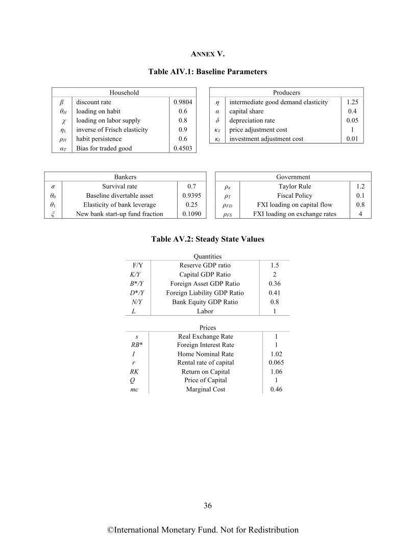
36

ANNEX V.

Table AIV.1: Baseline Parameters

Household Producers β discount rate 0.9804 η intermediate good demand elasticity 1.25 θH loading on habit 0.6 α capital share 0.4 χ loading on labor supply 0.8 δ depreciation rate 0.05

ηL inverse of Frisch elasticity 0.9 κY price adjustment cost 1 ρH habit persistence 0.6 κI investment adjustment cost 0.01 αT Bias for traded good 0.4503

Bankers Government σ Survival rate 0.7 ρπ Taylor Rule 1.2 θ0 Baseline divertable asset 0.9395 ρT Fiscal Policy 0.1 θ1 Elasticity of bank leverage 0.25 ρFD FXI loading on capital flow 0.8 ξ New bank start-up fund fraction 0.1090 ρFS FXI loading on exchange rates 4

Table AV.2: Steady State Values

Quantities F/Y Reserve GDP ratio 1.5

K/Y Capital GDP Ratio 2 B*/Y Foreign Asset GDP Ratio 0.36 D*/Y Foreign Liability GDP Ratio 0.41 N/Y Bank Equity GDP Ratio 0.8 L Labor 1

Prices

s RB*

Real Exchange Rate Foreign Interest Rate

1 1

I r

Home Nominal Rate Rental rate of capital

1.02 0.065

RK Q

Return on Capital Price of Capital

1.06 1

mc Marginal Cost 0.46


37

Figure AV.1: Impulse Responses to Capital Outflow Shock

Note: These figures show the impact of macrofinancial variables to a capital outflow shock under two scenarios: one with no FXI (blue lines) and the other with FXI (red lines).


38

Figure AV.2: Impulse Responses to Negative Productivity Shock

Note: These figures show the impact of macrofinancial variables to a decrease in productivity under two scenarios: one with no FXI (blue lines) and the other with FXI (red lines).


39

Table AV.3: Average Response to One Standard Deviation of Capital Outflow Shock Across Policies (in percentage)

Baseline FXI CFM MPM MP Output -0.61 -0.40 -0.40 -0.40 -0.40 Consumption Investment Labor Inflation FX rate FX borrowing Net worth

-0.27 -3.10 -0.46 -0.19 0.39 -6.70 -0.41

-0.14 -2.10 -0.30 -0.13 0.37 -8.20 -0.25

-0.19 -2.10 -0.32 -0.11 0.29 -4.20 -0.30

-0.19 -2.10 -0.31 -0.12 0.26 -7.70 -0.19

-0.16 -2.20 -0.26 0.96 0.31 -7.6 0.26


40

VII. REFERENCES

Abrigo, M.R.M and I. Love, 2016. "Estimation of Panel Vector Autoregression in Stata,” The Stata Journal, 778-804 (2016).

Ajello, A., T. Laubach, D. Lopez-Salido, and T. Nakata. 2019. “Financial Stability and Optimal Interest Rate Policy.” International Journal of Central Banking, 15(1): 279-326.

Alam, Z., A. Alter, J. Eiseman, G. Gelos, H. Kang, M. Narita, E. Nier, and N. Wang, 2019. “Digging Deeper—Evidence on the Effects of Macroprudential Policies from a New Database.” IMF Working Paper 19/66.

Albrizio, S., J. Flores and D. Furceri, (forthcoming). “Non-linear Macro and Distributional Effects of US Monetary Policy.”

Andrews, D. and B. Lu, 2001. “Consistent Model and Moment Selection Procedures for GMM Estimation with Application to Dynamic Panel Data Models,” Journal of Econometrics, 101(1), pp. 123-164.

Angeloni, I. & Faia, E., 2013. "Capital Regulation and Monetary Policy with Fragile banks," Journal of Monetary Economics, 60(3), pp. 311-324.

Aoki, K., G. Benigno, and N. Kiyotaki, 2016. “Monetary and financial policies in emerging markets.” Unpublished paper, London School of Economics.

Avdjiev, S., B. Hardy, S. Kalemli-Ozcan, and L. Servén, 2018. “Gross Capital Flows by Banks, Corporates and Sovereigns,” BIS Working Paper, No. 760.

Basu, S., E. Boz, G. Gopinath, F. Roch, and F. Unsal, 2020. “A Conceptual Model for the Integrated Policy Framework,” IMF Working Paper, No. 20/121.

Benes, J., A. Berg, R. Portillo, and D. Vavra, 2013. “Modeling Sterilized Interventions and Balance Sheet Effects of Monetary Policy in a New Keynesian Framework,” IMF Working Paper, No. 13/11.

Blanchard, O., G. Adler, I. de Carvalho Filho, 2015. “Can Foreign Exchange Intervention Stem Exchange Rate Pressures from Global Capital Flow Shocks?” NBER Working Paper 21427.

Brandao-Marques, Luis, G. Gelos, M. Narita, and E. Nier, 2020. “Leaning Against the Wind: A Cost-Benefit Analysis for an Integrated Policy Framework,” IMF Working Paper No. 20/123.

Bruno, V. and H. Shin, 2015. “Capital flows and the Risk-Taking Channel of Monetary Policy”, Journal of Monetary Economics, 71(15), pp. 119-132.

Cavallino, P., 2019. "Capital Flows and Foreign Exchange Intervention," American Economic Journal: Macroeconomics, American Economic Association, 11(2), pp. 127-170.


41

Cecchetti, S., T. Mancini-Griffoli, M. Narita, and R. Sahay, 2020. “U.S. or Domestic Monetary Policy: Which Matters More for Financial Stability?”, IMF Economic Review, 68(1), pp. 35-65.

Chamon, M., D. Hofman, N. Magud, and A. Werner, 2019. Foreign Exchange Intervention in Inflation Targeters in Latin America, International Monetary Fund: Washington, DC.

Chung, K., J. Lee, E. Loukoianova, H. Park, and H. Shin, 2014. “Global Liquidity through the Lens of Monetary Aggregates," IMF Working Paper, 14/9.

Corbacho, A., and S. Peiris (eds.), 2018. The ASEAN Way: Sustaining Growth and Stability, Washington, DC: International Monetary Fund.

Curdia, V. and M. Woodford, 2010. “Credit Spreads and Monetary Policy," Journal of Money, Credit and Banking, 2010, 42(6), pp 3-35.

Deb, P., S. Nadeem, and S. Peiris 2020. “The Transmission of External Shocks in Asia: Country Characteristics and Policy Responses,” IMF Working Paper, 20/3.

Escude, G., 2013. “A DSGE Model for a SOE with Systematic Interest and Foreign Exchange Policies in Which Policymakers Exploit the Risk Premium for Stabilization Purposes,” Economics: The Open-Access, Open-Assessment E-Journal, 7 (2013-30), pp. 1-110.

Filardo, A. and P. Rungcharoenkitkul, 2016. “A Quantitative Case for Leaning Against the Wind,” BIS Working Papers, No. 594.

Gabaix X, and M. Maggiori. “International Liquidity and Exchange Rate Dynamics,” Quarterly Journal of Economics, 130 (3), pp. 1369-1420.

Gambacorta, L., and F. M. Signoretti. 2014. “Should Monetary Policy Lean against the Wind?” Journal of Economic Dynamics and Control 43 (2014): 146–74.

Gelos, G., L. Gornicka, R. Koepke, R. Sahay, and S. Sgherri (2019). “Capital Flows at Risk: Taming the Ebbs and Flows,” IMF Working Paper 19/279.

Gertler, M., and P. Karadi, 2011. "A Model of Unconventional Monetary Policy," Journal of Monetary Economics, 58(1) pp. 17-34.

–––––, and N. Kiyotaki. 2015. "Banking, Liquidity, and Bank Runs in an Infinite Horizon Economy," American Economic Review, 105 (7), pp. 2011-43.

Ghilardi, M. and S. Peiris, 2014. " Capital Flows, Financial Intermediation and Macroprudential Policies," IMF Working Paper, No. 14/157.

Gopinath, G. 2015. “The International Price System.” In Jackson Hole Symposium, Volume 27. Kansas City: Federal Reserve Bank at Kansas City.


42

Hong, G., A. Oeking, K. Kang and C. Rhee, 2019. "What Do Deviations from Covered Interest Parity and Higher FX Hedging Costs Mean for Asia," IMF Working Paper, No. 19/169.

IMF, 2019a. “Facing the Tides: Managing Capital Flows in Asia.” APD Departmental Paper

–––––, 2019b. "Banks' Dollar Funding: A Source of Financial Vulnerability. Global Financial Stability Report, October 2019

Kalemli-Özcan, S., 2019. “U.S. Monetary Policy and International Risk Spillovers.” Jackson Hole Economic Policy Symposium.

Kannan, P., P. Rabanal, and A. Scott, 2012. "Monetary and Macroprudential Policy Rules in a Model with House Price Booms," The B.E. Journal of Macroeconomics, 12(1), pp. 1-44.

Kearns, J. and R. Rigobon, 2005. "Identifying The Efficacy Of Central Bank Interventions: Evidence From Australia And Japan," Journal of International Economics, 66(1), pp. 31-48.

Lane, P. and G. Milesi-Ferretti, 2017. " International Financial Integration in the Aftermath of the Global Financial Crisis," IMF Working Paper, No. 17/115.

Liu, Z. and M. Spiegel, 2015. "Optimal Monetary Policy and Capital Account Restrictions in a Small Open Economy," Federal Reserve Bank of San Francisco, Working Paper 2013-33.

Medina, J. and J. Roldos, 2014. " Monetary and Macroprudential Policies to Manage Capital Flows," IMF Working Paper, No. 14/30.

Menna, L. and M. Tobal, 2018. "Financial and Price Stability in Emerging Markets: The Role of the Interest Rate," BIS Working Paper, No. 717.

Mimir, Y, and Sunel, E., 2015. " External Shocks, Banks and Optimal Monetary Policy in an Open Economy," BIS Working Paper, No. 528.

Miranda-Agrippino, Silvia, and Hélène Rey. 2019. “Monetary Policy and the Global Financial Cycle.” NBER Working Paper No. 21722

Obstfeld, M., 2015. "Trilemmas and Tradeoffs: Living with Financial Globalization," BIS Working Paper, No 480.

–––––, J. Ostry, and M. Qureshi, 2019. “A Tie that Binds: Revisiting the Trilemma in Emerging Market Economies.” Review of Economics and Statistics, 101(2): 279–293

Oktiyanto, F., Harmanta, N. Purwanto, and A. Rachmanto, 2014. "Monetary Macroprudential Policy Mix under Financial Frictions Mechanism with DSGE Model," EcoMod2014 6840.


43

Ostry, J., A. Ghosh, and M. Chamon, 2012. "Two Targets, Two Instruments: Monetary and Exchange Rate Policies in Emerging Market Economies," IMF Staff Discussion Note, 12/01, International Monetary Fund, Washington, DC.

Rey, H., 2018. "Dilemma not Trilemma: The Global Financial Cycle and Monetary Policy Independence," NBER Working Paper No. 21162

Sahay, R., V. B. Arora, A. V. Arvanatis, H. Faruqee, P. N’Diaye, and T. Mancini-Griffoli. 2014. “Emerging Market Volatility: Lessons from the Taper Tantrum.” IMF Staff Discussion Note.

Shin, H., 2013. "Adapting Macro Prudential Approaches to Emerging and Developing Economies," in Dealing with the Challenges of Macro Financial Linkages in Emerging Markets, World Bank Group, Washington, DC.

Sims, C., 1980. "Macroeconomics and Reality," Econometrica, 48(1), pp. 1-48.

Unsal, F., 2013. " Capital Flows and Financial Stability: Monetary Policy and Macroprudential Responses," International Journal of Central Banking, 9(1), pp. 233-285.


wp/21/ - international monetary fund

Documents