wp spatial ieb 22 07 16 - dipòsit digital de la...

SPATIAL INTERACTION IN LOCAL EXPENDITURES AMONG ITALIAN

MUNICIPALITIES: EVIDENCE FROM ITALY 2001-2011

Massimiliano Ferraresi, Giuseppe Migali, Francesca Nordi, Leonzio Rizzo

IEB Working Paper 2016/22

Fiscal Federalism



MUNICIPALITIES: EVIDENCE FROM ITALY 2001-2011


The IEB research program in Fiscal Federalism aims at promoting research in the

public finance issues that arise in decentralized countries. Special emphasis is put on

applied research and on work that tries to shed light on policy-design issues. Research

that is particularly policy-relevant from a Spanish perspective is given special

consideration. Disseminating research findings to a broader audience is also an aim of

the program. The program enjoys the support from the IEB-Foundation and the IEB-

UB Chair in Fiscal Federalism funded by Fundación ICO, Instituto de Estudios Fiscales

and Institut d’Estudis Autonòmics.

The Barcelona Institute of Economics (IEB) is a research centre at the University of

Barcelona (UB) which specializes in the field of applied economics. The IEB is a

foundation funded by the following institutions: Applus, Abertis, Ajuntament de

Barcelona, Diputació de Barcelona, Gas Natural, La Caixa and Universitat de

Barcelona.

Postal Address:

Institut d’Economia de Barcelona

Facultat d’Economia i Empresa

Universitat de Barcelona

C/ John M. Keynes, 1-11

(08034) Barcelona, Spain

Tel.: + 34 93 403 46 46

[email protected]

http://www.ieb.ub.edu

The IEB working papers represent ongoing research that is circulated to encourage

discussion and has not undergone a peer review process. Any opinions expressed here

are those of the author(s) and not those of IEB.

mailto:[email protected]

http://www.ieb.ub.edu/



MUNICIPALITIES: EVIDENCE FROM ITALY 2001-2011*


ABSTRACT: We investigate the existence of spatial interaction in spending decisions

among Italian municipalities. We estimate a spatial autoregressive dynamic panel data

model, using information on 5,564 Italian municipalities over the period 2001-2011,

exploiting their border contiguity as a measure of spatial neighborhood. We find a

positive effect of neighboring expenditures on total, capital and current expenditures of

a given municipality. We do not find any evidence of yardstick competition when we

take account of political effects, while we find a negative relationship between spatial

interaction and the size of the municipality for current expenditure. Thus, we conclude

that spillover effects drive the strategic interaction.

JEL Codes: C23, H72

Keywords: Local public spending interaction, spillovers, yardstick competition,

spatial econometrics, dynamic panel data, system GMM.

Massimiliano Ferraresi

University of Ferrara

Department of Economics

and Management

Via Voltapaletto, 11

44121 Ferrara, Italy

e-mail: [email protected]

Giuseppe Migali

University of Lancaster & University

Magna Graecia


Bailrigg Lancaster, LA1 4YX, UK


Francesca Nordi

University of Messina & University

of Ferrara


and Management




Leonzio Rizzo

University of Ferrara & IEB


and Management




∗ Leonzio Rizzo thankfully acknowledge financial support from the Spanish Ministry of Economy and

Competitiveness (ECO2015-63591-R).





Introduction

Many studies in the last two decades aimed to assess the existence of spatial effects influencing local expenditure decisions. In particular, there is a line of empirical works (Case et al., 1993; Revelli, 2002; Revelli, 2003; Baicker, 2005; Solé-Ollé, 2006; Werck et al., 2008; Costa et al., 2015) that investigates whether governments make their spending decision taking into account the behavior of their neighbors. In such a framework, expenditures decisions would depend not only on income, grants, socio-demographic and political characteristics of municipalities, but also on spending decision of neighboring municipalities.

If municipalities choose their expenditures/taxes - which can affect the welfare of their neighbor’s – by maximizing their own welfare and so not taking into account their neighbor’s welfare they end up into inefficient levels of expenditure and/or taxes (Gordon, 1983). The existence of strategic interaction between municipalities is theoretically explained by several models, e.g. yardstick competition, tax and welfare competition, spillover effects (Brueckner, 2003; Revelli, 2005). In the yardstick competition model, voters with no complete information on the cost of public goods and services compare expenditures and taxes in their jurisdiction with those of nearby jurisdictions (Salomon, 1987). Therefore, the local policy makers mimic each other’s behavior. The second source of spatial interdependence arises in tax competition models. Municipalities face mobile tax bases, which depend on both their own tax rate and their neighbors’ tax rate giving rise to tax competition (Kanbur and Keen, 1993; Devereux et al., 2008; Rizzo, 2010). Finally, in the traditional “spillover” model, public expenditures of a municipality may have positive or negative effects beyond its own boundary, thus affecting the welfare of residents in neighboring municipalities (Case et al 1993; Revelli, 2002; Revelli, 2003; Baicker, 2005; Solé-Ollé, 2006; Werck et al., 2008; Costa et al., 2015). As a result, municipalities might decide the level of their own expenditure, by strategically taking into account the expenditures of their neighbors.

In our work, we first assess the existence of spatial effects influencing the expenditure decisions of Italian municipalities and then we identify the sources of this interdependence. We use information on all Italian municipalities (except for those in autonomous regions) over the period 2001-2011. By employing the Arellano-Bond estimator, we estimate an empirical model where the public expenditure in a given municipality depends on the average of their own border municipalities’ expenditures and on a set of control variables. We find a positive horizontal interdependence in spending decisions of Italian municipalities and we argue that this strategic interaction is mainly due to spillover effects and not to yardstick competition. However, some political variables turn out to be important determinants of local expenditure. In fact, the election year positively affects both total and current expenditure, implying the presence of a political budget cycle among Italian municipalities. Moreover, municipalities where the mayor wins the election with a strong majority, show higher level of expenditure. Finally, for current expenditure we find that the population size of the municipality negatively affects the impact of neighbors’ expenditure on its own expenditure, and above a certain population level the positive horizontal interdependence vanishes.

At the best of our knowledge, this is the first study on spatial interactions in local spending decisions, using data on all Italian municipalities. Bordignon et al. (2003) performed a spatial analysis of the Italian municipal property tax, by using data on municipalities belonging to the Lombardy region. They found that municipalities engage in yardstick competition when setting their property tax rate, but only when the mayor can run for re-election and the electoral outcome is uncertain. Ermini and Santolini (2010), found a positive and significant spillover effect for current expenditure, by relying on a sample of municipalities belonging to the Marche region. Finally, Santolini and Bartolini (2012), by using again a sample of municipalities belonging to the Marche region, found evidence of yardstick competition when they control for both the domestic stability pact and pre-electoral years.

2

The paper is organized as follows: Section 1 illustrates the institutional framework. Section 2 discusses the econometric strategy and Section 3 describes the data. Section 4, 5 and 6 illustrate the estimation results. Section 7 concludes.

1. Institutional framework: a brief analysis of Italian municipalities’ spending

The Italian Constitution defines four administrative government layers: central government, regions, provinces and municipalities. While most regions and provinces are ruled by ordinary statutes, some of them – the autonomous regions and provinces – are ruled by special statutes3. Furthermore, Italy counts 110 provinces, that have recently been reformed by the law 56/2014, which reduced their public competences and eliminated the possibility of direct elections of their own representatives. Finally, municipalities are the smallest level of jurisdiction and are around 8,000, although this number is decreasing because the law 56/2014 is incentivizing amalgamation. Most municipalities (around 90%) have less than 15,000 inhabitants and the average size is around 6,400 inhabitants.

Municipalities in Italy are responsible for several public functions such as social welfare services, territorial development, local transport, infant school education, sports and cultural facilities, local police services, water delivery, rubbish as well as most infrastructural spending. In our data, municipalities’ total expenditure accounts, on average, for about 8.7% of all total public expenditure in Italy during the period 2001-2011.

Municipalities’ current expenditure, on average, accounts for 71% of the municipalities’ total expenditure, which corresponds to 63 billion of euros per year during 2001-2011. Among current expenditure, approximately 75% is concentrated on four main functions: Administration and Management, Roads & Transport Services, Planning and Environment and Social welfare. The remaining 25% of the current expenditure is allocated to the Municipal police, Education, Culture, Sport, and Tourism. Finally, a very low amount of resources goes to three functions, Economic development, In-house production services and Justice, managed by many medium-sized and small municipalities networking with other municipalities.

Municipalities are also responsible for investments, which are on average 29% of the total expenditure in the period 2001-2011. However, it is worth noting that the share of these expenditures sharply decreased in the period 2006-2011, switching from 34% to 21% of total expenditures. At the same time, the share of current expenditure has increased. Looking at the specific functions, municipalities allocate resources for investments mainly to Administration and Management (16.7% of the capital expenditure) Roads & Transport Services (26%), Planning and Environment (27.5%) and Education (9%).

2. Empirical framework

Our econometric strategy is based on the estimation of a spatial autoregressive dynamic panel model (Anselin et al., 2008), which takes the following form:

!"# = % + '!("#)*) + ,-!)"# + ./"# + 0" + 1# + 2"#, (1)

where !"# is the per capita expenditure of municipality i at year t, and !("#)*) is its one year lagged value.

3 In Italy there are five autonomous regions (Sicilia and Sardegna, which are insular territories, and Valle d’Aosta, Trentino Alto Adige and Friuli Venezia Giulia, which are northern boundary territories) and two autonomus provinces (Trento and Bolzano).

3

-!)",# = ∑ 5"6!6#67" is the weighted per capita average expenditure of the neighboring municipalities j at timet; ω9: are exogenously chosen weights that aggregate the per capita expenditure of neighboring municipalitiesinto a single variable WG)9,=. The ω9: are normalized so that ∑ ω9::79 = 1. /"# is a matrix of exogenousdemographic, socio-economic and political characteristics of municipality i at time t. µi is an unobservedmunicipal specific effect, τt is a year specific intercept and εit is a mean zero, normally distributed random error.

In equation (1), the coefficient β measures the degree of inertia of the municipal expenditure. Whereas thecoefficient γ captures the horizontal interdependence in the municipal expenditure, that is the reaction of theexpenditure of a given municipality to a one-euro increase in the average expenditure of its neighbors. There are three possible cases:

i) γ =0: no horizontal interdependence.ii) γ< 0: negative horizontal interdependence. A one-euro increase in the average expenditure of

neighboring municipalities leads to a reduction in the municipal expenditure.iii) γ> 0: positive horizontal interdependence. A one-euro increase in the average expenditure of

neighboring municipalities leads to an increase in the municipal expenditure.

Since equation (1) includes endogenous variables, the OLS estimation is inappropriate and generates biased estimates. The average neighboring expenditure, -!)"#, is endogenous because expenditure interactions aresymmetric and simultaneous: each municipalities’ behavior affects that of its neighbors and it is affected by their behavior in the same way. The lagged dependent variable, !("#)*), which is an important determinant of themunicipal expenditure (Veiga and Veiga, 2007; Larcinese et al., 2013), is correlated with the municipality fixed effects in the error term, leading to biased and inconsistent fixed effects estimations (Nickell, 1981). Thus, we use the system GMM (SYS-GMM) dynamic panel estimator (Arellano and Bover,1995; Blundell and Bond, 1998).

This estimator is an augmented version of the difference GMM (Arellano and Bond, 1991) and is considered more efficient (Blundell and Bond, 1998). The SYS-GMM, differently from the difference GMM which just employs the difference equation, builds a stacked dataset, one in levels and one in differences. Then the differences equations are instrumented with levels, while the levels equations are instrumented with differences4.

The consistency of the GMM estimator depends on the assumption that the error term is serially uncorrelated, otherwise the instruments are not valid. Hence, to check for the absence of first-order serial correlation in levels in a dataset expressed in differences, as that used in a SYS-GMM, we need to check for the absence of second order correlation in differences. In fact, we are able to detect first order serial correlation in level between 2"#)*and 2"#)A by looking at the correlation between ∆2"#(∆2"# = 2"# − 2"#)*) and ∆2"#)A(∆2"#)A = 2"#)A − 2"#)D).For this reason, we test, using the differenced estimating equation, for first order autoregressive (AR(1)) serial correlation in the residuals, which we expect negative and significant5 and for second order autoregressive (AR(2)) serial correlation in the residuals, which we expect not significant (Arellano and Bond, 1991), where in both tests the null hypothesis is the absence of serial correlation in the residuals.6

4 As a generic example, consider the following model in first difference: ∆E"# = %∆E"#)* + ∆F"#G ' + ∆H"#, then the term E"#)* in ∆E"#)*(∆E"#)* = E"#)* − E"#)A) is correlated with the term H"#)* in ∆H"# (∆H"# = H"# − H"#)*), so the choice of E"#)* as instrument would biasthe estimates. As a results, for the equation in differences, we may use lagged values of E"# to form instruments as long as E"#is laggedtwo periods or more (E"#)A, E"#)D ,… ). Notice that, for other endogenous variables, the natural candidate instrument for ∆F"# is F"#)A, thesecond lag of endogenous variable, which again is not correlated to the error term ∆H"#. As concerns the level equations, the laggedendogenous variables (E"#)*) can be instrumented with ∆E"#)* since it is not correlated with H"#. For the same reason, if F"# isendogenous, ∆F"#)* (∆F"#)* = F"#)* − F"#)A), is a valid instrument since it is not correlated with the error term H"#.5 Since ∆2"# is analytically related to ∆2"#)* via the term 2"#)*, a negative first-order serial correlation is always expected in differences. Infact, E(∆2"#, ∆2"#)*)=E(2"# − 2"#)*) E (2"#)* − 2"#)A) = -Var2"#)*.

6 In fact E(∆2"#, ∆2"#)A)=E(2"# − 2"#)*) E (2"#)A − 2"#)D) =0.

4

In order to check the validity of the instruments, we employ the standard Hansen test whose null hypothesis is the exogeneity of the corresponding instrument (or group of instruments). However, as Roodman (2009) points out, the power of the Hansen test might be weakened if the number of instruments is high. Consequently, we test the validity of a subset of instruments by using a C-test (Baum, 2006). The C-test estimates the SYS-GMM with and without a subset of instruments and uses the difference between the two respective Hansen tests distributed as a chi2 and, allowing to test the null hypothesis that the excluded instrument are valid, namely they are exogenous.

The SYS-GMM requires an additional assumption with respect to the difference GMM: the first differenced instruments for the level equations must be not correlated with the fixed effects. For this reason we apply the C-test to the level equation and so comparing the Hansen test of this last equation with that of the SYS-GMM. The null hypothesis is that the instruments (which are taken in difference) for the level equations are valid and so the SYS-GMM is preferred to the difference GMM.

Finally, we use a two-step SYS-GMM, which makes the covariance matrix more robust to panel specific autocorrelation and heteroskedasticity, so the estimator is more efficient (Arellano and Bond, 1991; Blundell and Bond 1998). However, by using this procedure the standard errors might be severely downward biased (Roodman, 2009), hence, in order to correct the bias, we apply the correction made by Windmeijer (2005).

3. Data

The data on Italian municipalities used in our work result from a combination of different archives provided by the Italian Ministry of Internal Affairs, the Ministry of Economy and the Institute of National Statistics.

The data so obtained include a full range of information for the period 2001-2011 and are organized into two sections: 1) municipality financial data and 2) municipality demographic, socio-economic and electoral data, such as population size, age structure, average income of inhabitants, years of election. We restrict our sample to municipalities located in ordinary statute regions. We exclude municipalities that have a specific status of metropolitan areas (law 56/2014)7, because they usually provide a wider range of services compared to other municipalities. Our final sample includes 5,564 municipalities8, observed from 2001 to 2011, which generates a balanced panel data set of 61,204 observations.

All financial variables are expressed in 2011 real per capita value.

The Italian municipality balance sheet reports expenditures either in accrual basis or in cash basis. In this system of public accountability there is usually a gap (exceeding, sometimes, more than one financial year) between the payment (registered on cash basis) and the commitment to it (registered on accrual basis). For this reason, we prefer to use the cash basis classification, since the value is reported only if the payment has effectively been made.

3.1 Dependent variables and variables of interest.

We estimate equation (1) using three different dependent variables: per capita total expenditure (total expenditure), per capita current expenditure (current expenditure) and, per capita capital expenditure (capital expenditure). We use these aggregate measures of expenditure and not those disaggregated by functions, because many municipalities (especially the small ones) have expenditure crossing more than one function, but often registered only in one function.

7 Milano, Roma, Napoli, Torino, Bari, Firenze, Bologna, Genova, Venezia and Reggio Calabria. 8 We have removed all those municipalities with missing values in the dependent variables defined at section 3.l.

5

To isolate the independent impact of neighboring expenditures on the expenditure of a given municipality, we use the neighbors’ expenditures variable (neigh expenditure). In order to obtain this variable, as mentioned in Section 2, we use a contiguity matrix, implying 5"6 = 1/J" where J" is the number of municipalitiescontiguous to i and 5"6 = 0 otherwise. Hence, for each municipality i in period t, the average value of its ownneighbors’ per capita expenditure is given by -!)",# = ∑ 5"6!6#67" .

3.2 Control variables

The municipality expenditure can be affected by other factors, accounting for demographic, socio-economic and electoral characteristics. In particular, we include a set of time-varying variables, which characterizes the municipality’s demographic and economic situation. We include municipality population (population/100) and per capita area (area) - square kilometers divided by population - which can capture the presence of scale economies and/or congestion effects. The proportion of citizens aged between 0 and 5 (children) and the proportion of citizens aged over 65 (aged) can control for some specific public needs (e.g., nursery school, nursing homes for the elderly).

In terms of economic and financial controls, we include the per capita personal income tax base (income/100), i.e. a proxy of per capita average income, and per capita transfers (current, capital or total grants) from upper tiers of governments (transfers), that vary according to the dependent variable adopted in the estimation.9 The variable transfers might also be endogenous as simultaneously decided with municipalities’ expenditures, and we take into account this potential issue by applying the SYS-GMM.

Furthermore, we use a set of political variables that may influence local budgets. In particular, we define a dummy variable (election), which is equal to 1 for a given municipality in the year of election, during the period 2001-2011. We measure the political power of the mayor by using the percentage of votes that have been necessary to win an election (vote-share). Since Italian law establishes a limit of no more than two consecutive terms in office for a mayor, we use a dummy variable (term-limit) which is equal to 1 for all the years a mayor is at her second term (and hence she cannot be re-elected) and it is equal to 0 when the mayor is at her first term.

From 200110, the Italian central government – in order to fulfill the obligations of the European Stability and Growth Pact – imposes to each municipality above 5,000 inhabitants the so-called Domestic Stability Pact. Depending on the year, it implies a constrained municipal deficit or a threshold on the municipal expenditure. Hence, we include a dummy (domestic stability pact) equal to one if a municipality has to fulfill the Domestic Stability Pact (i.e. it has more than 5,000 inhabitants) and 0 otherwise.

The summary statistics of all the variables used in the analysis are reported in Table 1.

9 In the year 2008-2011 we subtract the compensative transfer from the central state that has been introduced to replace the missing revenue from the abolished property tax on owner-occupied dwellings.

10 See law 388/2000, article 53.

6

Table 1.Summary statistics

Variable Number of observations Mean Standard

deviation. Minimum Maximum

Total expenditure 61,204 1,251.95 1,101.98 30.17 43,906.23 Current expenditure 61,204 742.04 390.06 5.63 13,023.92 Capital expenditure 61,204 509.91 851.44 0 42,127.01 Total transfers 61,204 620.43 834.36 7.14 33,814.22 Current transfers 61,204 277.61 234.39 1.10 14,177.54 Capital transfers 61,204 342.82 714.18 0.00 32,906.61 Population/100 61,204 64.75 13.97 0.04 2653.68 Children (0-5 years old) 61,204 0.05 0.01 0 0.13 Aged (>65 years old) 61,204 0.22 0.06 0.04 0.63 Area 61,204 0.02 0.04 0 1.15 Income/100 61,204 109.34 36.79 2.13 1965.78 Domestic stability pact 61,204 0.31 0.46 0 1 Election 61,204 0.20 0.40 0 1 Term-limit 61,204 0.38 0.49 0 1 Vote-share 61,204 0.59 0.16 0.16 1 Notes: All the variables are averages for the period 2001-2011. The financial variables are in real, per capita and cash flows terms. Children, aged, area and income are divided by population.

4. Results

We first estimate equation (1) by using the OLS estimator, with and without neighboring expenditure variable (col. 1 and 2, Table 2), then we replicate the previous estimation by applying the FE estimator (col. 3 and 4, Table 2) and, finally, we perform the SYS-GMM estimator (col. 5 and 6, Table 2).

The coefficient of the lagged dependent variable in the OLS estimation without the neighboring expenditure (col. 1, Table 2), is positive (0.52) and statistically significant at 1% level, implying that expenditure shows a certain degree of inertia. This is also confirmed when we introduce the neighboring expenditure (neigh expenditure), whose coefficient, which accounts for the spatial interdependence of municipal expenditures, is positive (0.08) and statistically significant at 1% (col. 2, Table 2).

These results remain the same when we include municipality fixed effects. In particular, without neighboring expenditure, the estimated coefficient of the lagged dependent variable is positive (0.26) and statistically significant at 1% (col. 3, Table 2). When we include the neighboring expenditure, its estimated coefficient is positive (0.11), statistically significant at 1% (col. 4, Table 2) and higher than that obtained by using the OLS.

As previously discussed, the estimation of equation (1) by both OLS and FE estimators leads to biased and inconsistent estimations, hence we apply the SYS-GMM estimator. In this case the coefficient of the lagged dependent variable is positive and statistically significant at 1%, both in the specification without neighboring expenditure (0.32; col. 5, Table 2) and in that with neighboring expenditure (0.31; col. 6, Table 2). This confirms the inertia of the municipal expenditure. The coefficient of neighboring expenditure is positive (0.16) and statistically significant at 10%. What this simply suggests is that there is a positive horizontal interdependence in the expenditure of Italian municipalities, such that a one-euro increase in the average expenditure of the neighbors generates, ceteris paribus, an increase in the expenditure of municipality i of 0.16 euro.

Looking at the other control variables, we find that the coefficient of total transfers is always positive in all specifications. In particular, in the SYS-GMM (col. 6; Table 2), the estimated coefficient of total transfers is

7

positive (0.38) and statistically significant at 1%, implying that grants have an important impact on spending decision at the municipal level.11 Moreover, municipalities’ geographic and demographic characteristics have also an effect on total expenditures. The coefficient of per capita area (area) is positive and statistically significant at 1% (col. 6; Table 2), suggesting that a 50% increase of per capita area (e.g. from its average value of 0.02 to 0.03) would increase per capita expenditure by 43.09 euro. The variable area per capita captures the effect of economies of scale, i.e. the less populated a municipality is the higher the expenditure.

The coefficient of population (population/100) is positive (0.12) and statistically significant at 1% (col. 6; Table 2), accounting for the presence of congestion effects. Per capita income of residents (income/100) has a coefficient of around 1.79, statistically significant at 1% (col. 6, Table 2).

The coefficient of children is negative and highly significant, and it implies that an increase of children’s share in the population by, for example, 20% (from the average value of 0.05 to 0.06) corresponds to a reduction of 20.23 euro in the per capita expenditure. This is also an economy of scale effect.

All our specifications include political and institutional variables as well. Focusing on the SYS-GMM, the dummy variable election has a positive coefficient (20.24), vote-share is also positive (75.86) and they are both significant at 1% (col. 6, Table 2). Finally, the dummy variable domestic stability pact shows a negative coefficient (-38.08) and statistically significant at 1% (col. 6, Table 2). This result confirms the strength of the Domestic Stability Pact in constraining local expenditures, in line with recent findings (Grembi et al., 2016).12

11 Transfers from upper level of government represent a significant part, appoximatley around 25%, of the Italian municipal financing system.

12 This result should be read with some warning. In fact, the variable domestic stability pact (which is 0 if population is lower than 5,000 inhabitants and 1 otherwise) also accounts for other municipal rules. For example the mayor’s salary and the amount of transfers received from the central government change if the municipality is above the threshold of 5,000 inhabitants.

In Table 3 we report the results of the estimations using as dependent variable the two components of total expenditures: current expenditure (col. 1) and capital expenditure (col. 2). We only apply our favorite econometric model, the SYS-GMM, with the specification including the neighbors’ expenditure. We still instrument our lagged dependent variable and the other endogenous variables (neigh expenditure and transfers). Looking at the estimates for current expenditure (col. 1, Table 3), the coefficient of the lagged dependent variable is positive (0.11), statistically significant at 10% and smaller than the one estimated for total expenditure (col. 6, Table 2). The estimated coefficient associated with current expenditure of neighboring muncipalities (neigh expenditure) is positive (0.65), statistically significant at 1% and increases considerably with respect to the one estimated for total expenditure.

8

Table 2 Estimation results for total expenditure with OLS, FE estimator and SYS-GMM

(1) (2) (3) (4) (5) (6) Dependent variable Total expenditure Total expenditure Total expenditure Total expenditure Total expenditure Total expenditure Model OLS OLS FE FE SYS-GMM SYS-GMM

Expenditure (-1) 0.52*** 0.50*** 0.26*** 0.25*** 0.32*** 0.31*** (0.03) (0.03) (0.03) (0.03) (0.06) (0.06)

Neigh expenditure 0.08*** 0.11*** 0.16* (0.01) (0.02) (0.10)

Transfers 0.55*** 0.54*** 0.61*** 0.60*** 0.41*** 0.38*** (0.03) (0.03) (0.04) (0.04) (0.09) (0.10)

Population/100 0.10*** 0.06*** -2.15*** -1.90*** 0.10*** 0.12*** (0.01) (0.01) (0.40) (0.38) (0.02) (0.02)

Children -1,406.81*** -1,410.96*** -1,115.82 -1,068.08 -2,055.45*** -2,023.64*** (416.62) (414.55) (774.43) (766.87) (551.51) (517.72)

Aged -200.26* -311.72*** 74.93 98.73 478.51*** 228.99 (120.79) (112.81) (307.60) (302.87) (181.54) (243.16)

Area 1,793.84*** 1,469.89*** 9,070.05*** 8,637.67*** 5,351.47*** 4,309.18*** (310.08) (308.65) (3,405.03) (3,280.87) (641.12) (949.25)

Income/100 2.16*** 2.15*** 3.46*** 3.33*** 1.90*** 1.79*** (0.13) (0.13) (0.83) (0.82) (0.33) (0.39)

Domestic stability pact -9.99** -6.23 -77.19*** -73.39** -49.52*** -38.08*** (4.40) (4.08) (28.96) (29.09) (9.82) (11.04)

Election 11.59** 11.66** 22.54*** 22.13*** 20.86*** 20.24*** (4.89) (4.85) (3.93) (3.92) (4.52) (4.87)

Term-limit 1.98 3.11 7.30* 7.15* 1.52 3.03 (4.01) (3.10) (4.15) (4.14) (3.95) (3.96)

Vote-share 4.69 4.32 20.18 21.43 88.70*** 75.86*** (15.87) (15.82) (20.69) (20.73) (27.91) (28.11)

Constant 149.47*** 104.7*** 189.42 69.40 287.19*** 181.99** (35.38) (36.37) (155.31) (155.64) (49.79) (73.11)

Number of observations 55,640 55,640 55,640 55,640 55,640 55,640 R-squared 0.83 0.84 0.45 0.46 Number of municipalities 5,564 5,564 AR1 (p-value) 0.00 0.00 Hansen (p-value) 0.78 0.50 AR2 (p-value) 0.86 0.73

Notes: *** p < 0.01, ** p < 0.05, * p < 0.1 Robust standard errors in parentheses. In all regressions, we control for time fixed effects. In regression (3), (4), (5) and (6) we also control for municipal fixed effects. In regression (5) and (6) Expenditure (-1), neigh expenditure and total transfers are instrumented using SYS-GMM. In col. (5) the variable Expenditure (-1) is instrumented applying difference GMM, by using lags 1, 2 and 3; the variable transfers (total transfers) is instrumented applying SYS-GMM by using lags 3 and 4. In col. (6) the variable Expenditure (-1) is instrumented applying difference GMM by using lags 1, 2 and 3; the variable neigh expenditure is instrumented applying SYS-GMM, by using lags 3 and 4; the variable transfers (total transfers) is instrumented applying SYS-GMM by using lags 3 and 4. The validity of the instruments is checked by using the standard Hansen test and the C test (results are available upon request).

9

Moving to capital expenditure (col. 2, Table 3), the estimated coefficient of the lagged dependent variable is positive (0.31), statistically significant at 1% and very similar to the one estimated for total expenditure (col. 6, Table 2). The coefficient of capital expenditure of neighboring muncipalities is sligthly lower than the one estimated for total expenditure (0.10), and statistically significant at 5%.

These results suggest the presence of positive horizontal interdependence of both current and capital expenditure among Italian municipalities, and such an effect is more pronounced for current expenditure. Indeed, a one-euro increase in the average current expenditure of the neighbors generates, ceteris paribus, an increase of 0.65 euro in the municipality’s current expenditure. Whereas, a one-euro increase in the average capital expenditures of the neighbors generates, ceteris paribus, an increase of 0.10 euro in municipality’s capital expenditure.

Control variables are also very informative about the determinants of both current and capital municipal expenditure. In particular, the coefficient associated with population/100 is positive and statistically significant, showing the presence of congestion effects, and the coefficient of per-capita area (area) is positive and statistically significant, implying the presence of economies of scale. The coefficient associated with vote-share is positive and statistically significant and the dummy variable domestic stability pact shows a negative and significant (at 1%) coefficient.

Other control variables, such as current transfers, income/100 and election are not statistically significant when using current expenditure (col. 1, Table 3). When we use capital expenditure (col. 2, Table 3), the coefficients of capital transfers (0.47), income/100 (0.26) and election (17.57) are all positive and significant at 1%.

To sum up, all our results show the presence of a positive horizontal interdependence in spending decision among Italian municipalities, especially for current expenditure. We also find a degree of inertia of the expenditure. Furthermore, political variables are important factors of municipal expenditure. The percentage of votes (vote-share) obtained by a mayor in an election is always statistically significant and positively impacts on expenditures. This means that a mayor with a strong majority in a municipality council spends more than a mayor with a weak leadership. In the year of election, we find an increase of total expenditure, driven by capital expenditure.

4.1 Robustness check

We re-estimate the previous models by using different neighbor’s matrices. In particular, we define this new neighbors’ variable (neigh expenditure) by using two weighted matrices. We first consider neighbors all municipalities distant up to 25 km from a given municipality and we weigh the corresponding expenditure with the inverse of that distance; above 25 km the weight is 0. Then, by using the same procedure, we classify as neighbors all municipalities whose distance from a given municipality is no more than 50 km.

We perform the estimations for the total expenditure and its two components (current expenditure and capital expenditure) using the two spatial matrices, separately. The estimates obtained using a neighbor’s distance less than 25 km confirm the results we have obtained in the previous analysis (col. 1, 2 and 3, Table 4). The strategic interaction between expenditures persists with each type of expenditure. The coefficient of neighboring expenditure (neigh expenditure) is 0.22 and significant at 10% when using total expenditure, and it is very similar (0.20) for capital expenditure; however it becomes significant at 1% and increases to 0.77 with current expenditure. When we use a neighbor’s distance up to 50 km, the estimates confirm again our previous results, for all types of expenditure (col. 4, 5 and 6, Table 4). Precisely, when we use total expenditure (col. 4, Table 4) the coefficient of neighbor’s expenditure (neigh expenditure) is 0.34 and statistically significant at 1%. In the other two cases, neighboring expenditures have coefficients of 0.88 (at 1% significance) and 0.21 (at 10% significance), for current and capital expenditures, respectively.

10

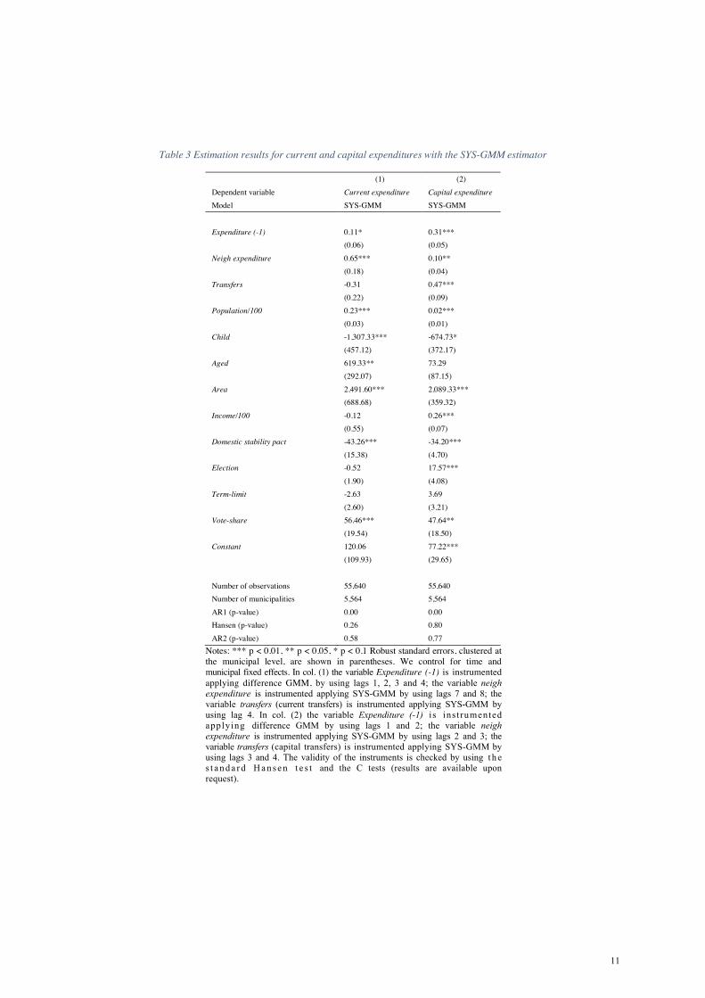
Table 3 Estimation results for current and capital expenditures with the SYS-GMM estimator

(1) (2)Dependent variable Current expenditure Capital expenditure Model SYS-GMM SYS-GMM

Expenditure (-1) 0.11* 0.31*** (0.06) (0.05)

Neigh expenditure 0.65*** 0.10** (0.18) (0.04)

Transfers -0.31 0.47*** (0.22) (0.09)

Population/100 0.23*** 0.02*** (0.03) (0.01)

Child -1,307.33*** -674.73* (457.12) (372.17)

Aged 619.33** 73.29 (292.07) (87.15)

Area 2,491.60*** 2,089.33*** (688.68) (359.32)

Income/100 -0.12 0.26*** (0.55) (0.07)

Domestic stability pact -43.26*** -34.20*** (15.38) (4.70)

Election -0.52 17.57*** (1.90) (4.08)

Term-limit -2.63 3.69 (2.60) (3.21)

Vote-share 56.46*** 47.64** (19.54) (18.50)

Constant 120.06 77.22*** (109.93) (29.65)

Number of observations 55,640 55,640 Number of municipalities 5,564 5,564 AR1 (p-value) 0.00 0.00 Hansen (p-value) 0.26 0.80 AR2 (p-value) 0.58 0.77

Notes: *** p < 0.01, ** p < 0.05, * p < 0.1 Robust standard errors, clustered at the municipal level, are shown in parentheses. We control for time and municipal fixed effects. In col. (1) the variable Expenditure (-1) is instrumented applying difference GMM, by using lags 1, 2, 3 and 4; the variable neigh expenditure is instrumented applying SYS-GMM by using lags 7 and 8; the variable transfers (current transfers) is instrumented applying SYS-GMM by using lag 4. In col. (2) the variable Expenditure (-1) i s ins t rumented applying difference GMM by using lags 1 and 2; the variable neigh expenditure is instrumented applying SYS-GMM by using lags 2 and 3; the variable transfers (capital transfers) is instrumented applying SYS-GMM by using lags 3 and 4. The validity of the instruments is checked by using t h e s t a n d a r d H a n s e n t e s t and the C tests (results are available upon request).

11

Table 4. Estimation results for total, current and capital expenditure with SYS-GMM using different type of neighbors’ matrices

(1) (2) (3) (4) (5) (6)

Weighting matrix -ALMN -LOMN

Dependent variable Total expenditure Current expenditure

Capital expenditure Total expenditure Current

expenditure Capital expenditure

Model SYS-GMM SYS-GMM SYS-GMM SYS-GMM SYS-GMM SYS-GMM

Expenditure (-1) 0.35*** 0.10* 0.34*** 0.31*** 0.15 0.33***

(0.06) (0.06) (0.07) (0.06) (0.22) (0.06)

Neigh expenditure 0.22* 0.77*** 0.20* 0.34*** 0.88*** 0.21**

(0.12) (0.20) (0.11) (0.12) (0.29) (0.10)

Transfers 0.31*** -0.22 0.40*** 0.36*** -0.21 0.47***

(0.10) (0.23) (0.11) (0.09) (0.37) (0.09)

Population/100 0.12*** 0.22*** 0.03*** 0.11*** 0.19*** 0.02*

(0.02) (0.03) (0.01) (0.02) (0.07) (0.01)

Child -2,270.74*** -1,317.45*** -611.47 -1,946.55*** -1,244.68* -842.77**

(566.61) (440.09) (393.31) (525.01) (684.46) (393.44)

Aged 154.45 454.63 45.03 30.08 334.33 -44.46

(249.82) (298.53) (120.89) (231.42) (405.33) (120.55)

Area 4,650.75*** 2,632.93*** 2,221.82*** 4,916.38*** 3,069.51*** 2,041.17***

(833.76) (614.97) (440.93) (774.87) (1,153.48) (406.78)

Income/100 1.72*** 0.21 0.32*** 1.91*** 0.14 0.38***

(0.36) (0.57) (0.10) (0.31) (0.84) (0.10)

Domestic stability pact -33.69** -28.14* -26.63*** -28.33** -27.12 -26.93***

(13.66) (15.90) (8.11) (12.37) (22.48) (7.25)

Election 19.36*** -0.96 17.17*** 20.51*** -0.84 18.15***

(4.71) (2.15) (4.28) (4.67) (2.75) (4.09)

Term-limit 4.13 -2.63 3.67 3.59 -3.71 3.10

(3.91) (2.56) (3.25) (3.91) (4.28) (3.25)

Vote-share 94.28*** 45.12** 50.91*** 80.98*** 37.47 50.38***

(26.43) (20.30) (17.23) (27.31) (32.73) (18.33)

Constant 124.69 19.46 39.36 -19.18 -68.83 41.52

(117.91) (118.79) (51.86) (121.60) (106.10) (55.89)

Number of observations 55,640 55,640 55,640 55,640 55,640 55,640

Number of municipalities 5,564 5,564 5,564 5,564 5,564 5,564

AR1 (p-value) 0.00 0.00 0.00 0.00 0.04 0.00

Hansen (p-value) 0.83 0.18 0.50 0.38 0.23 0.58

AR2 (p-value) 0.76 0.89 0.72 0.70 0.89 0.84

Notes: *** p < 0.01, ** p < 0.05, * p < 0.1 Robust standard errors, clustered at the municipal level, are shown in parentheses. We control for time and municipal fixed effects. The variables neigh expenditure and transfers are always instrumented using SYS-GMM, instead Expenditure (-1) in all the regressions is instrumented using difference GMM. Instruments: (1) lags 1 and 2 for the variable Expenditure (-1), lags 4 and 5 for the variables neigh expenditure and transfers (total transfers); (2) lags 1, 2, 3 and for the variable Expenditure (-1), lags 7 and 8 for the variable neigh expenditure, lags 4 and 5 for the variable transfers (current transfers); (3) lags 1, 2, 3 and 4 for the variable Expenditure (-1), lags 4 and 5 for the variable neigh expenditure and lag 4 for the variable transfers (capital transfers); (4) lags 1 and 2 for the variable Expenditure (-1), lags 3 and 4 for the variable neigh expenditure and for the variable transfers (total transfers); (5) lags 1 for the variable Expenditure (-1), lags 4, 5 and 6 for the variable neigh expenditure and lag 5 for the variable transfers (current transfers); (6) lags 1, 2 and 3 for the variable Expenditure (-1), 4 and 5 for the variable neigh expenditure and lags 3 and 4 for the variable transfers (capital transfers). The validity of the instruments is checked by using the standard Hansen test and the C tests (results are available upon request).

12

The estimates presented so far show that there is a strategic interaction between spending decisions at local level. This feature holds for both current and capital expenditure. The presence of strategic interaction might be reasonably due to the fact that citizens living in the neighboring municipalities can enjoy the provision of local public goods in a given municipality. This implies the presence of spillover effects (Case et al., 1993). However, the strategic interaction can also be justified by yardstick competition between municipalities (Besley and Case, 1995): voters judge expenditure levels (and so local public good provision) by looking at what comparable municipalities do.

The empirical studies on yardstick competition link the spending interaction with the political process. In particular, they assume that the interdependence may be effective in pre-electoral and electoral years (Bordignon et al., 2003; Solé-Ollé, 2003), when politicians mimic the behavior of their neighbor’s to capture voters’ preferences and to win the elections. This behavior is more pronounced when politicians are not lame duck, which implies that they are interested in obtaining voters’ confidence (Bordignon et al., 2003). Voters with no complete information about the type of incumbent, in fact, compare their municipal expenditures with those of nearby municipalities (Salmon, 1987).

We test whether the spatial interaction found in the baseline regressions is due to yardstick competition, by interacting the neighboring expenditure variable with political dummies. Therefore, we consider the following model:

!"# = % + '!("#)*) + ,-!)"# + P(QRSTUTVWS_YZJJE"# ∗ -!)"#) + ./"# + 0" + 1# + 2"#. (2)

We estimate equation (2) using SYS-GMM and instrumenting our lagged dependent variable and the other endogenous variables (neighboring expenditure, neigboring expenditure interacted with political dummy and transfers). We separately estimate equation (2) using two different specifications where in one case we use as political dummy term-limit and in the other case we use election. As dependent variable we cosider the total expenditure and its two components (current expenditure and capital expenditure). In the first specification (Table 5), if there is yardstick competition we expect the interaction between term-limit and neighbors’ expenditure to be negative, because a lame-duck mayor should not have any electoral concern. However, the interaction term (neigh expenditure*termlim) is not statistically significant for total (col. 1), current (col. 2) and capital (col. 3) expenditures.

5. Testing for political sources of the interdependence

In the second specification (Table 6), we expect the interaction between election and neighbors’ expenditure to be positive (Costa et al., 2015). However, the interaction term (neigh expenditure*election) is never statistically significant.

These results reveal the absence of yardstick competition as source of interaction: municipalities do not mimic each other to get votes and the spatial interdependence is not sensitive to the electoral cycle. Thus, we can conclude that the strategic interaction found in the baseline specification is due to spillovers of the provided public goods.

13

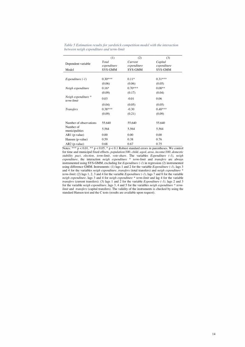
Table 5 Estimation results for yardstick competition model with the interaction between neigh expenditure and term-limit

(1) (2) (3)

Dependent variable Total expenditure

Current expenditure

Capital expenditure

Model SYS-GMM SYS-GMM SYS-GMM

Expenditure (-1) 0.30*** 0.11* 0.31*** (0.06) (0.06) (0.05)

Neigh expenditure 0.16* 0.70*** 0.08**(0.09) (0.17) (0.04)

Neigh expenditure * term-limit 0.03 -0.01 0.06

(0.04) (0.05) (0.05) Transfers 0.38*** -0.30 0.48***

(0.09) (0.21) (0.09)

Number of observations 55,640 55,640 55,640 Number of municipalities 5,564 5,564 5,564

AR1 (p-value) 0.00 0.00 0.00 Hansen (p-value) 0.59 0.38 0.76 AR2 (p-value) 0.68 0.67 0.75

Notes: *** p < 0.01, ** p < 0.05, * p < 0.1 Robust standard errors in parentheses. We control for time and municipal fixed effects, population/100, child, aged, area, income/100, domestic stability pact, election, term-limit, vote-share. The variables Expenditure (-1), neigh expenditure, the interaction neigh expenditure * term-limit and transfers are always instrumented using SYS-GMM, excluding for Expenditure (-1) in regression (2) instrumented using difference GMM. Instruments: (1) lags 1 and 2 for the variable Expenditure (-1), lags 3 and 4 for the variables neigh expenditure, transfers (total transfers) and neigh expenditure * term-limit; (2) lags 1, 2, 3 and 4 for the variable Expenditure (-1), lags 7 and 8 for the variable neigh expenditure, lags 3 and 4 for neigh expenditure * term-limit and lag 4 for the variable transfers (current transfers); (3) lags 1 and 2 for the variable Expenditure (-1), lags 2 and 3 for the variable neigh expenditure, lags 3, 4 and 5 for the variables neigh expenditure * term-limit and transfers (capital transfers). The validity of the instruments is checked by using the standard Hansen test and the C tests (results are available upon request).

14

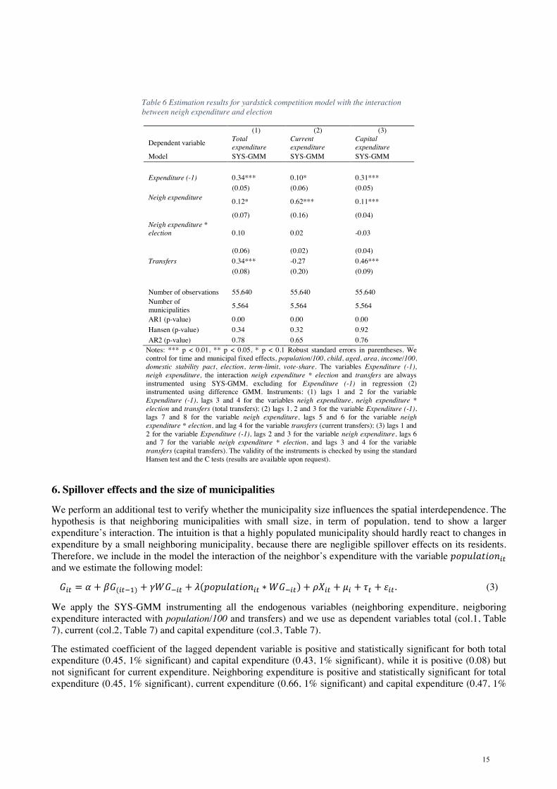
Table 6 Estimation results for yardstick competition model with the interaction between neigh expenditure and election

(1) (2) (3)

Dependent variable Total expenditure

Current expenditure

Capital expenditure

Model SYS-GMM SYS-GMM SYS-GMM

Expenditure (-1) 0.34*** 0.10* 0.31*** (0.05) (0.06) (0.05)

Neigh expenditure 0.12* 0.62*** 0.11***

(0.07) (0.16) (0.04) Neigh expenditure * election 0.10 0.02 -0.03

(0.06) (0.02) (0.04) Transfers 0.34*** -0.27 0.46***

(0.08) (0.20) (0.09)

Number of observations 55,640 55,640 55,640 Number of municipalities 5,564 5,564 5,564

AR1 (p-value) 0.00 0.00 0.00 Hansen (p-value) 0.34 0.32 0.92 AR2 (p-value) 0.78 0.65 0.76

Notes: *** p < 0.01, ** p < 0.05, * p < 0.1 Robust standard errors in parentheses. We control for time and municipal fixed effects, population/100, child, aged, area, income/100, domestic stability pact, election, term-limit, vote-share. The variables Expenditure (-1), neigh expenditure, the interaction neigh expenditure * election and transfers are always instrumented using SYS-GMM, excluding for Expenditure (-1) in regression (2) instrumented using difference GMM. Instruments: (1) lags 1 and 2 for the variable Expenditure (-1), lags 3 and 4 for the variables neigh expenditure, neigh expenditure * election and transfers (total transfers); (2) lags 1, 2 and 3 for the variable Expenditure (-1), lags 7 and 8 for the variable neigh expenditure, lags 5 and 6 for the variable neigh expenditure * election, and lag 4 for the variable transfers (current transfers); (3) lags 1 and 2 for the variable Expenditure (-1), lags 2 and 3 for the variable neigh expenditure, lags 6

and 7 for the variable neigh expenditure * election, and lags 3 and 4 for the variable transfers (capital transfers). The validity of the instruments is checked by using the standard Hansen test and the C tests (results are available upon request).

6. Spillover effects and the size of municipalities

We perform an additional test to verify whether the municipality size influences the spatial interdependence. The hypothesis is that neighboring municipalities with small size, in term of population, tend to show a larger expenditure’s interaction. The intuition is that a highly populated municipality should hardly react to changes in expenditure by a small neighboring municipality, because there are negligible spillover effects on its residents. Therefore, we include in the model the interaction of the neighbor’s expenditure with the variable QRQZSWUTR\"#and we estimate the following model:

!"# = % + '!("#)*) + ,-!)"# + ](QRQZSWUTR\"# ∗ -!)"#) + ./"# + 0" + 1# + 2"#. (3)

We apply the SYS-GMM instrumenting all the endogenous variables (neighboring expenditure, neigboring expenditure interacted with population/100 and transfers) and we use as dependent variables total (col.1, Table 7), current (col.2, Table 7) and capital expenditure (col.3, Table 7).

The estimated coefficient of the lagged dependent variable is positive and statistically significant for both total expenditure (0.45, 1% significant) and capital expenditure (0.43, 1% significant), while it is positive (0.08) but not significant for current expenditure. Neighboring expenditure is positive and statistically significant for total expenditure (0.45, 1% significant), current expenditure (0.66, 1% significant) and capital expenditure (0.47, 1%

15

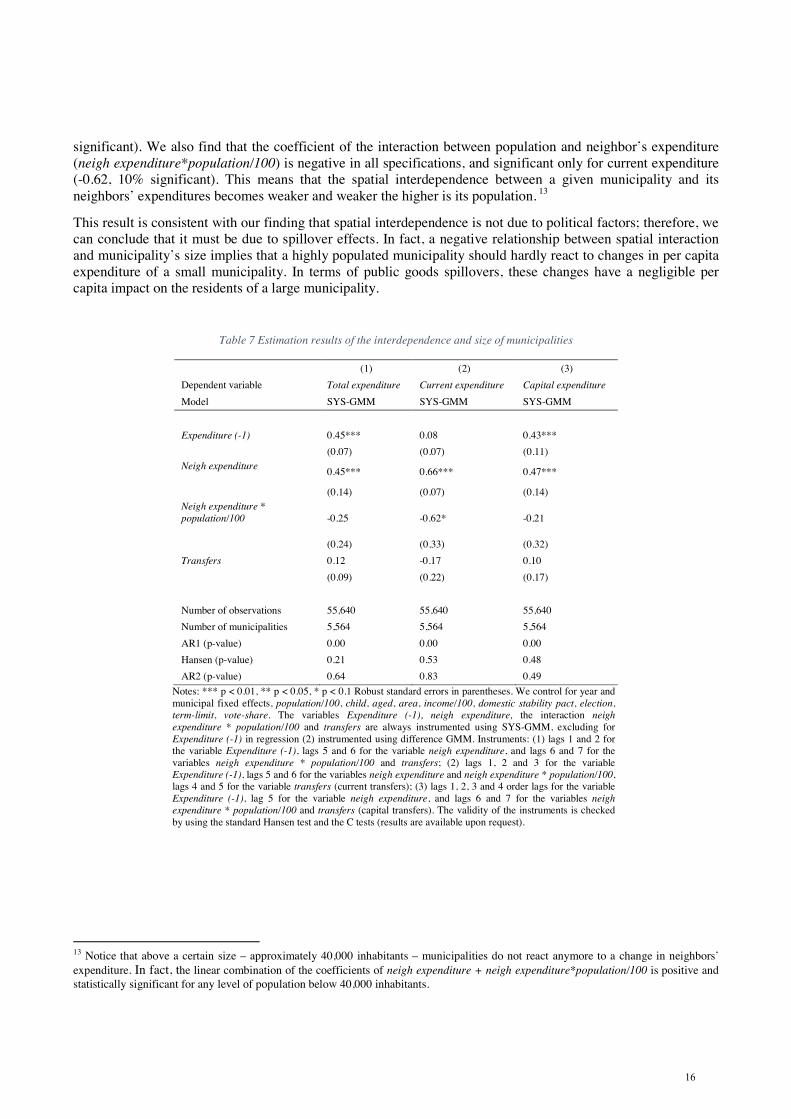
significant). We also find that the coefficient of the interaction between population and neighbor’s expenditure (neigh expenditure*population/100) is negative in all specifications, and significant only for current expenditure (-0.62, 10% significant). This means that the spatial interdependence between a given municipality and its neighbors’ expenditures becomes weaker and weaker the higher is its population. 13

This result is consistent with our finding that spatial interdependence is not due to political factors; therefore, we can conclude that it must be due to spillover effects. In fact, a negative relationship between spatial interaction and municipality’s size implies that a highly populated municipality should hardly react to changes in per capita expenditure of a small municipality. In terms of public goods spillovers, these changes have a negligible per capita impact on the residents of a large municipality.

Table 7 Estimation results of the interdependence and size of municipalities

(1) (2) (3) Dependent variable Total expenditure Current expenditure Capital expenditure Model SYS-GMM SYS-GMM SYS-GMM

Expenditure (-1) 0.45*** 0.08 0.43*** (0.07) (0.07) (0.11)

Neigh expenditure 0.45*** 0.66*** 0.47***

(0.14) (0.07) (0.14) Neigh expenditure * population/100 -0.25 -0.62* -0.21

(0.24) (0.33) (0.32) Transfers 0.12 -0.17 0.10

(0.09) (0.22) (0.17)

Number of observations 55,640 55,640 55,640 Number of municipalities 5,564 5,564 5,564 AR1 (p-value) 0.00 0.00 0.00 Hansen (p-value) 0.21 0.53 0.48 AR2 (p-value) 0.64 0.83 0.49

Notes: *** p < 0.01, ** p < 0.05, * p < 0.1 Robust standard errors in parentheses. We control for year and municipal fixed effects, population/100, child, aged, area, income/100, domestic stability pact, election, term-limit, vote-share. The variables Expenditure (-1), neigh expenditure, the interaction neigh expenditure * population/100 and transfers are always instrumented using SYS-GMM, excluding for Expenditure (-1) in regression (2) instrumented using difference GMM. Instruments: (1) lags 1 and 2 for the variable Expenditure (-1), lags 5 and 6 for the variable neigh expenditure, and lags 6 and 7 for the variables neigh expenditure * population/100 and transfers; (2) lags 1, 2 and 3 for the variable Expenditure (-1), lags 5 and 6 for the variables neigh expenditure and neigh expenditure * population/100, lags 4 and 5 for the variable transfers (current transfers); (3) lags 1, 2, 3 and 4 order lags for the variable Expenditure (-1), lag 5 for the variable neigh expenditure, and lags 6 and 7 for the variables neigh expenditure * population/100 and transfers (capital transfers). The validity of the instruments is checked by using the standard Hansen test and the C tests (results are available upon request).

13 Notice that above a certain size – approximately 40,000 inhabitants – municipalities do not react anymore to a change in neighbors’ expenditure. In fact, the linear combination of the coefficients of neigh expenditure + neigh expenditure*population/100 is positive and statistically significant for any level of population below 40,000 inhabitants.

16

7. Conclusion

In this paper we explored the existence of spatial interactions in spending decisions among Italian municipalities. We estimated a spatial autoregressive dynamic panel data model, by using data on 5,564 Italian municipalities for the period 2001-2011, and exploiting their border contiguity. We found a positive and statistically significant effect of neighbors’ expenditure on the expenditure of a given municipality, for total, capital and current expenditure. We did not find any evidence of yardstick competition, and therefore we are confident that spillover effects drive the strategic interaction. This conclusion is confirmed by the results of a negative relationship between spatial interaction and municipality’s size for current expenditures. A highly populated municipality should hardly react to changes in per capita expenditure of a small municipality, because public goods spillovers are negligible on the residents of a large municipality.

Appendix

Dependent variables

• ^FQ_\YTUZ`_"# (total, current, capital); !",#. Per capita expenditures of municipality i at time t, expressed in2011 Euros and in cash flow terms. These financial data are taken from the official municipality balancesheets available on http://finanzalocale.interno.it/ser/i_banchedati.html provided by the Italian Ministry ofInternal Affairs.

Endogenous variables

• a_Tbℎ_FQ_\YTUZ`_"# (total, current, capital) ; -!)",# = ∑ 5"6!6#67" . It is the per capita averageexpenditure of neighboring municipalities of the municipality i at time t, expressed in 2011 Euros and incash flow terms. The concept of neighbors varies across specifications of the model: border municipalities,25 km distant municipalities and 50 km distant municipalities.

• ^FQ_\YTUZ`_(−1)"#(URUWS, VZ``_\U, VWQTUWS); !",#)*. One year lagged value of the variable^FQ_\YTUZ`_"#.

• e`W\fg_`f"# (total, current and capital). Per capita upper tier governments’ transfers to municipality i attime t, expressed in 2011 Euros and in cash flow terms. These financial data are taken from the officialmunicipality balance sheets. Transfers vary according to the dependent variable adopted in the estimation.For the years 2008-2011 we subtract the compensative transfer from the central government that has beenintroduced to replace the missing revenue from the abolished property tax on owner-occupied dwellings.

Demographic and socio-economic variables

• hRQZSWUTR\/100"# is the number of inhabitants of municipality i at time t, taken fromhttp://www.istat.it/it/archivio/113712 provided by the Institute of National Statistics.

• iℎTSY`_\"# is the ratio of individuals aged 0-5 years to the total population of municipality i at time t, takenfrom http://www.istat.it/it/archivio/113712 provided by the Institute of National Statistics.

• jb_Y"# is the ratio of individuals over 65 years of age to the total population of municipality i at time t,taken from http://www.istat.it/it/archivio/113712 provided by the Institute of National Statistics.

• j`_W"# is the area of the municipality i divided by its own population. Area data were taken fromhttp://www.istat.it/it/archivio/113712 provided by the Institute of National Statistics.

• k\VRJ_/100"# is the per capita income for municipality i at time t. Income data were taken from theMinistry of Economy.

• ^S_VUTR\"# dummy=1 in the year of election. Data are taken from http://elezionistorico.interno.it/ providedby the Italian Ministry of Internal Affairs.

17

• e_`J− STJTU"# dummy=1 if the mayor cannot run for reelection, taken from http://elezionistorico.interno.it/provided by the Italian Ministry of Internal Affairs.

• lRU_ − fℎW`_"# is the percentage share of the mayor in the vote for the election. If a municipality have morethan 15,000 inhabitants and the electoral system is a double ballot system, the vote-share refers to the firstround of election. Data are taken from http://elezionistorico.interno.it/ provided by the Italian Ministry ofInternal Affairs.

• mRJ_fUTVfUWnTSTUEQWVU"# dummy=1 if a municipality is imposed the Domestic Stability Pact, namely ithas more than 5,000 inhabitants.

References

Anselin, L., Le Gallo, J., & Jayet, H. (2008). Spatial panel econometrics. In The econometrics of panel data (pp. 625-660). Springer Berlin Heidelberg.

Arellano, M. and Bover, O. (1995) Another look at the instrumental variable estimation of error-components models, Journal of Econometrics, 68(1): 29-51

Arellano, M. and Bond, S. (1991) Some Tests of Specification for Panel Data: Monte Carlo Evidence and an Application to Employment Equations, Review of Economic Studies, 58: 277-297

Baicker, K. (2005). The spillover effects of state spending. Journal of public economics, 89(2): 529-544.

Bartolini, D. and Santolini, R. (2012) Political yardstick competition among Italian municipalities on spending decisions, Annals of Regionals Science, 49:213-235, DOI 10.1007/s00168-011-0437-5

Baum, C. F. (2006). An introduction to modern econometrics using Stata. Stata press.

Besley, T. and Case A. (1995). Does electoral accountability affect economic policy choices? Evidence from gubernatorial term limits, The Quarterly Journal of Economics, 769-798

Blundell, R. and Bond, S. (1998) Initial conditions and moment restrictions in dynamic panel data models, Journal of Econometrics, 87: 115-143

Bordignon, M., Cerniglia, F. and Revelli, F. (2003) In search of yardstick competition: a spatial analysis of Italian municipality property tax setting, Journal of Urban Economics, 54: 199-217

Brueckner, J. K. (2003). Strategic interaction among governments: An overview of empirical studies. International regional science review, 26(2): 175-188.

Case, A. C., Hines, J. R. J. and Rosen H. S. (1993) Budget spillovers and fiscal policy interdependence. Evidence from the states, Journal of Public Economics, 52: 285-307

Costa, H., Veiga, G. and Portela, M. (2015) Interactions in Local Governments’ Spending Decisions: Evidence from Portugal, Regional Studies, 49:9, 144-1456, DOI: 10.1080/00343404.2013.835798

Devereux, M. P., Lockwood, B. and Redoano, M. (2008) Do countries compete over corporate tax rates?, Journal of Public Economics, 92(5-6): 1210-1235

Ermini, B. and Santolini, R. (2010) Local Expenditure interaction in Italian municipalities: do local partnership make a difference?, Local Government Studies, 36(5), 655-677

Gordon R. H. (1983) An optimal taxation approach to fiscal federalism, Quarterly Journal of Economics, 98, 567-587.

18

Grembi, V., Nannicini, T. and Troiano, U. (2016) "Do Fiscal Rules Matter?" American Economic Journal: Applied Economics, 8(3): 1-30. DOI: 10.1257/app.20150076

Kanbur, R. and Keen, M. (1993) Jeux Sans Frontieres: Tax Competition and Tax Coordination When Countries Differ in Size, American Economic Review, 83(4): 877-92

Larcinese, V., Rizzo, L. and Testa, C. (2013). Why Do Small States Receive More Federal Money? U.S. Senate Representation and the Allocation of Federal Budget, Economics and Politics, 25(3): 257-282

Nickell, S. (1981) Biases in Dynamic Models with Fixed Effects, Econometrica, 49(6):1417-1426

Solé-Ollé, A. (2003). Electoral accountability and tax mimicking: the effects of electoral margins, coalition government, and ideology. European Journal of Political Economy, 19(4): 685-713.

Solé-Ollé, A. (2006). Expenditure spillovers and fiscal interactions: Empirical evidence from local governments in Spain. Journal of Urban Economics, 59(1): 32-53.

Revelli, F. (2002) Testing the tax mimicking versus expenditure spillover hypotheses using English data, Applied Economics, 34:14, 1723-1731. DOI:10.1080/00036840210122353

Revelli, F. (2003) Reaction or interaction? Spatial process identification in multi-tiered government structures, Journal of Urban Economics, 53: 29-53, DOI:10.1016/S0094-1190(02)00512-0

Revelli, F. (2005) On Spatial Public Finance Empirics, International Tax and Public Finance, 12: 4751-1492

Rizzo, L. (2010). Interaction between federal taxation and horizontal tax competition: theory and evidence from Canada. Public Choice, 144(1-2): 369-387.

Roodman, D. (2009). A note on the theme of too many instruments. Oxford Bulletin of Economics and statistics, 71(1): 135-158.

Salmon, P. (1987) Decentralisation as an Incentive Scheme, Oxford Review of Economic Policy, Oxford University Press, 3(2): 24-43

Veiga, L. and Veiga, F. (2007) Political business cycles at the municipal level, Public Choice, 131(1): 45-64

Werck, K., Heyndels, B., & Geys, B. (2008). The impact of ‘central places’ on spatial spending patterns: evidence from Flemish local government cultural expenditures. Journal of Cultural Economics, 32(1): 35-58.

Windmeijer, F. (2005). A finite sample correction for the variance of linear efficient two-step GMM estimators. Journal of econometrics, 126(1), 25-51.

19

IEB Working Papers

2012

2012/1, Montolio, D.; Trujillo, E.: "What drives investment in telecommunications? The role of regulation, firms’

internationalization and market knowledge"

2012/2, Giesen, K.; Suedekum, J.: "The size distribution across all “cities”: a unifying approach"

2012/3, Foremny, D.; Riedel, N.: "Business taxes and the electoral cycle"

2012/4, García-Estévez, J.; Duch-Brown, N.: "Student graduation: to what extent does university expenditure

matter?"

2012/5, Durán-Cabré, J.M.; Esteller-Moré, A.; Salvadori, L.: "Empirical evidence on horizontal competition in

tax enforcement"

2012/6, Pickering, A.C.; Rockey, J.: "Ideology and the growth of US state government"

2012/7, Vergolini, L.; Zanini, N.: "How does aid matter? The effect of financial aid on university enrolment

decisions"

2012/8, Backus, P.: "Gibrat’s law and legacy for non-profit organisations: a non-parametric analysis"

2012/9, Jofre-Monseny, J.; Marín-López, R.; Viladecans-Marsal, E.: "What underlies localization and

urbanization economies? Evidence from the location of new firms"

2012/10, Mantovani, A.; Vandekerckhove, J.: "The strategic interplay between bundling and merging in

complementary markets"

2012/11, Garcia-López, M.A.: "Urban spatial structure, suburbanization and transportation in Barcelona"

2012/12, Revelli, F.: "Business taxation and economic performance in hierarchical government structures"

2012/13, Arqué-Castells, P.; Mohnen, P.: "Sunk costs, extensive R&D subsidies and permanent inducement

effects"

2012/14, Boffa, F.; Piolatto, A.; Ponzetto, G.: "Centralization and accountability: theory and evidence from the

Clean Air Act"

2012/15, Cheshire, P.C.; Hilber, C.A.L.; Kaplanis, I.: "Land use regulation and productivity – land matters:

evidence from a UK supermarket chain"

2012/16, Choi, A.; Calero, J.: "The contribution of the disabled to the attainment of the Europe 2020 strategy

headline targets"

2012/17, Silva, J.I.; Vázquez-Grenno, J.: "The ins and outs of unemployment in a two-tier labor market"

2012/18, González-Val, R.; Lanaspa, L.; Sanz, F.: "New evidence on Gibrat’s law for cities"

2012/19, Vázquez-Grenno, J.: "Job search methods in times of crisis: native and immigrant strategies in Spain"

2012/20, Lessmann, C.: "Regional inequality and decentralization – an empirical analysis"

2012/21, Nuevo-Chiquero, A.: "Trends in shotgun marriages: the pill, the will or the cost?"

2012/22, Piil Damm, A.: "Neighborhood quality and labor market outcomes: evidence from quasi-random

neighborhood assignment of immigrants"

2012/23, Ploeckl, F.: "Space, settlements, towns: the influence of geography and market access on settlement

distribution and urbanization"

2012/24, Algan, Y.; Hémet, C.; Laitin, D.: "Diversity and local public goods: a natural experiment with exogenous

residential allocation"

2012/25, Martinez, D.; Sjögren, T.: "Vertical externalities with lump-sum taxes: how much difference does

unemployment make?"

2012/26, Cubel, M.; Sanchez-Pages, S.: "The effect of within-group inequality in a conflict against a unitary threat"

2012/27, Andini, M.; De Blasio, G.; Duranton, G.; Strange, W.C.: "Marshallian labor market pooling: evidence

from Italy"

2012/28, Solé-Ollé, A.; Viladecans-Marsal, E.: "Do political parties matter for local land use policies?"

2012/29, Buonanno, P.; Durante, R.; Prarolo, G.; Vanin, P.: "Poor institutions, rich mines: resource curse and the

origins of the Sicilian mafia"

2012/30, Anghel, B.; Cabrales, A.; Carro, J.M.: "Evaluating a bilingual education program in Spain: the impact

beyond foreign language learning"

2012/31, Curto-Grau, M.; Solé-Ollé, A.; Sorribas-Navarro, P.: "Partisan targeting of inter-governmental transfers

& state interference in local elections: evidence from Spain"

2012/32, Kappeler, A.; Solé-Ollé, A.; Stephan, A.; Välilä, T.: "Does fiscal decentralization foster regional

investment in productive infrastructure?"

2012/33, Rizzo, L.; Zanardi, A.: "Single vs double ballot and party coalitions: the impact on fiscal policy. Evidence

from Italy"

2012/34, Ramachandran, R.: "Language use in education and primary schooling attainment: evidence from a

natural experiment in Ethiopia"

2012/35, Rothstein, J.: "Teacher quality policy when supply matters"

2012/36, Ahlfeldt, G.M.: "The hidden dimensions of urbanity"

2012/37, Mora, T.; Gil, J.; Sicras-Mainar, A.: "The influence of BMI, obesity and overweight on medical costs: a

panel data approach"

2012/38, Pelegrín, A.; García-Quevedo, J.: "Which firms are involved in foreign vertical integration?"

IEB Working Papers

2012/39, Agasisti, T.; Longobardi, S.: "Inequality in education: can Italian disadvantaged students close the gap? A

focus on resilience in the Italian school system"

2013

2013/1, Sánchez-Vidal, M.; González-Val, R.; Viladecans-Marsal, E.: "Sequential city growth in the US: does age

matter?"

2013/2, Hortas Rico, M.: "Sprawl, blight and the role of urban containment policies. Evidence from US cities"

2013/3, Lampón, J.F.; Cabanelas-Lorenzo, P-; Lago-Peñas, S.: "Why firms relocate their production overseas?

The answer lies inside: corporate, logistic and technological determinants"

2013/4, Montolio, D.; Planells, S.: "Does tourism boost criminal activity? Evidence from a top touristic country"

2013/5, Garcia-López, M.A.; Holl, A.; Viladecans-Marsal, E.: "Suburbanization and highways: when the Romans,

the Bourbons and the first cars still shape Spanish cities"

2013/6, Bosch, N.; Espasa, M.; Montolio, D.: "Should large Spanish municipalities be financially compensated?

Costs and benefits of being a capital/central municipality"

2013/7, Escardíbul, J.O.; Mora, T.: "Teacher gender and student performance in mathematics. Evidence from

Catalonia"

2013/8, Arqué-Castells, P.; Viladecans-Marsal, E.: "Banking towards development: evidence from the Spanish

banking expansion plan"

2013/9, Asensio, J.; Gómez-Lobo, A.; Matas, A.: "How effective are policies to reduce gasoline consumption?

Evaluating a quasi-natural experiment in Spain"

2013/10, Jofre-Monseny, J.: "The effects of unemployment benefits on migration in lagging regions"

2013/11, Segarra, A.; García-Quevedo, J.; Teruel, M.: "Financial constraints and the failure of innovation

projects"

2013/12, Jerrim, J.; Choi, A.: "The mathematics skills of school children: How does England compare to the high

performing East Asian jurisdictions?"

2013/13, González-Val, R.; Tirado-Fabregat, D.A.; Viladecans-Marsal, E.: "Market potential and city growth:

Spain 1860-1960"

2013/14, Lundqvist, H.: "Is it worth it? On the returns to holding political office"

2013/15, Ahlfeldt, G.M.; Maennig, W.: "Homevoters vs. leasevoters: a spatial analysis of airport effects"

2013/16, Lampón, J.F.; Lago-Peñas, S.: "Factors behind international relocation and changes in production

geography in the European automobile components industry"

2013/17, Guío, J.M.; Choi, A.: "Evolution of the school failure risk during the 2000 decade in Spain: analysis of

Pisa results with a two-level logistic mode"

2013/18, Dahlby, B.; Rodden, J.: "A political economy model of the vertical fiscal gap and vertical fiscal

imbalances in a federation"

2013/19, Acacia, F.; Cubel, M.: "Strategic voting and happiness"

2013/20, Hellerstein, J.K.; Kutzbach, M.J.; Neumark, D.: "Do labor market networks have an important spatial

dimension?"

2013/21, Pellegrino, G.; Savona, M.: "Is money all? Financing versus knowledge and demand constraints to

innovation"

2013/22, Lin, J.: "Regional resilience"

2013/23, Costa-Campi, M.T.; Duch-Brown, N.; García-Quevedo, J.: "R&D drivers and obstacles to innovation in

the energy industry"

2013/24, Huisman, R.; Stradnic, V.; Westgaard, S.: "Renewable energy and electricity prices: indirect empirical

evidence from hydro power"

2013/25, Dargaud, E.; Mantovani, A.; Reggiani, C.: "The fight against cartels: a transatlantic perspective"

2013/26, Lambertini, L.; Mantovani, A.: "Feedback equilibria in a dynamic renewable resource oligopoly: pre-

emption, voracity and exhaustion"

2013/27, Feld, L.P.; Kalb, A.; Moessinger, M.D.; Osterloh, S.: "Sovereign bond market reactions to fiscal rules

and no-bailout clauses – the Swiss experience"

2013/28, Hilber, C.A.L.; Vermeulen, W.: "The impact of supply constraints on house prices in England"

2013/29, Revelli, F.: "Tax limits and local democracy"

2013/30, Wang, R.; Wang, W.: "Dress-up contest: a dark side of fiscal decentralization"

2013/31, Dargaud, E.; Mantovani, A.; Reggiani, C.: "The fight against cartels: a transatlantic perspective"

2013/32, Saarimaa, T.; Tukiainen, J.: "Local representation and strategic voting: evidence from electoral boundary

reforms"

2013/33, Agasisti, T.; Murtinu, S.: "Are we wasting public money? No! The effects of grants on Italian university

students’ performances"

2013/34, Flacher, D.; Harari-Kermadec, H.; Moulin, L.: "Financing higher education: a contributory scheme"

2013/35, Carozzi, F.; Repetto, L.: "Sending the pork home: birth town bias in transfers to Italian municipalities"

IEB Working Papers

2013/36, Coad, A.; Frankish, J.S.; Roberts, R.G.; Storey, D.J.: "New venture survival and growth: Does the fog

lift?"

2013/37, Giulietti, M.; Grossi, L.; Waterson, M.: "Revenues from storage in a competitive electricity market:

Empirical evidence from Great Britain"

2014

2014/1, Montolio, D.; Planells-Struse, S.: "When police patrols matter. The effect of police proximity on citizens’

crime risk perception"

2014/2, Garcia-López, M.A.; Solé-Ollé, A.; Viladecans-Marsal, E.: "Do land use policies follow road

construction?"

2014/3, Piolatto, A.; Rablen, M.D.: "Prospect theory and tax evasion: a reconsideration of the Yitzhaki puzzle"

2014/4, Cuberes, D.; González-Val, R.: "The effect of the Spanish Reconquest on Iberian Cities"

2014/5, Durán-Cabré, J.M.; Esteller-Moré, E.: "Tax professionals' view of the Spanish tax system: efficiency,

equity and tax planning"

2014/6, Cubel, M.; Sanchez-Pages, S.: "Difference-form group contests"

2014/7, Del Rey, E.; Racionero, M.: "Choosing the type of income-contingent loan: risk-sharing versus risk-

pooling"

2014/8, Torregrosa Hetland, S.: "A fiscal revolution? Progressivity in the Spanish tax system, 1960-1990"

2014/9, Piolatto, A.: "Itemised deductions: a device to reduce tax evasion"

2014/10, Costa, M.T.; García-Quevedo, J.; Segarra, A.: "Energy efficiency determinants: an empirical analysis of

Spanish innovative firms"

2014/11, García-Quevedo, J.; Pellegrino, G.; Savona, M.: "Reviving demand-pull perspectives: the effect of

demand uncertainty and stagnancy on R&D strategy"

2014/12, Calero, J.; Escardíbul, J.O.: "Barriers to non-formal professional training in Spain in periods of economic

growth and crisis. An analysis with special attention to the effect of the previous human capital of workers"

2014/13, Cubel, M.; Sanchez-Pages, S.: "Gender differences and stereotypes in the beauty"

2014/14, Piolatto, A.; Schuett, F.: "Media competition and electoral politics"

2014/15, Montolio, D.; Trillas, F.; Trujillo-Baute, E.: "Regulatory environment and firm performance in EU

telecommunications services"

2014/16, Lopez-Rodriguez, J.; Martinez, D.: "Beyond the R&D effects on innovation: the contribution of non-

R&D activities to TFP growth in the EU"

2014/17, González-Val, R.: "Cross-sectional growth in US cities from 1990 to 2000"

2014/18, Vona, F.; Nicolli, F.: "Energy market liberalization and renewable energy policies in OECD countries"

2014/19, Curto-Grau, M.: "Voters’ responsiveness to public employment policies"

2014/20, Duro, J.A.; Teixidó-Figueras, J.; Padilla, E.: "The causal factors of international inequality in co2

emissions per capita: a regression-based inequality decomposition analysis"

2014/21, Fleten, S.E.; Huisman, R.; Kilic, M.; Pennings, E.; Westgaard, S.: "Electricity futures prices: time

varying sensitivity to fundamentals"

2014/22, Afcha, S.; García-Quevedo, J,: "The impact of R&D subsidies on R&D employment composition"

2014/23, Mir-Artigues, P.; del Río, P.: "Combining tariffs, investment subsidies and soft loans in a renewable

electricity deployment policy"

2014/24, Romero-Jordán, D.; del Río, P.; Peñasco, C.: "Household electricity demand in Spanish regions. Public

policy implications"

2014/25, Salinas, P.: "The effect of decentralization on educational outcomes: real autonomy matters!"

2014/26, Solé-Ollé, A.; Sorribas-Navarro, P.: "Does corruption erode trust in government? Evidence from a recent

surge of local scandals in Spain"

2014/27, Costas-Pérez, E.: "Political corruption and voter turnout: mobilization or disaffection?"

2014/28, Cubel, M.; Nuevo-Chiquero, A.; Sanchez-Pages, S.; Vidal-Fernandez, M.: "Do personality traits affect

productivity? Evidence from the LAB"

2014/29, Teresa Costa, M.T.; Trujillo-Baute, E.: "Retail price effects of feed-in tariff regulation"

2014/30, Kilic, M.; Trujillo-Baute, E.: "The stabilizing effect of hydro reservoir levels on intraday power prices

under wind forecast errors"

2014/31, Costa-Campi, M.T.; Duch-Brown, N.: "The diffusion of patented oil and gas technology with

environmental uses: a forward patent citation analysis"

2014/32, Ramos, R.; Sanromá, E.; Simón, H.: "Public-private sector wage differentials by type of contract:

evidence from Spain"

2014/33, Backus, P.; Esteller-Moré, A.: "Is income redistribution a form of insurance, a public good or both?"

2014/34, Huisman, R.; Trujillo-Baute, E.: "Costs of power supply flexibility: the indirect impact of a Spanish

policy change"

IEB Working Papers

2014/35, Jerrim, J.; Choi, A.; Simancas Rodríguez, R.: "Two-sample two-stage least squares (TSTSLS) estimates

of earnings mobility: how consistent are they?"

2014/36, Mantovani, A.; Tarola, O.; Vergari, C.: "Hedonic quality, social norms, and environmental campaigns"

2014/37, Ferraresi, M.; Galmarini, U.; Rizzo, L.: "Local infrastructures and externalities: Does the size matter?"

2014/38, Ferraresi, M.; Rizzo, L.; Zanardi, A.: "Policy outcomes of single and double-ballot elections"

2015

2015/1, Foremny, D.; Freier, R.; Moessinger, M-D.; Yeter, M.: "Overlapping political budget cycles in the

legislative and the executive"

2015/2, Colombo, L.; Galmarini, U.: "Optimality and distortionary lobbying: regulating tobacco consumption"

2015/3, Pellegrino, G.: "Barriers to innovation: Can firm age help lower them?"

2015/4, Hémet, C.: "Diversity and employment prospects: neighbors matter!"

2015/5, Cubel, M.; Sanchez-Pages, S.: "An axiomatization of difference-form contest success functions"

2015/6, Choi, A.; Jerrim, J.: "The use (and misuse) of Pisa in guiding policy reform: the case of Spain"

2015/7, Durán-Cabré, J.M.; Esteller-Moré, A.; Salvadori, L.: "Empirical evidence on tax cooperation between

sub-central administrations"

2015/8, Batalla-Bejerano, J.; Trujillo-Baute, E.: "Analysing the sensitivity of electricity system operational costs

to deviations in supply and demand"

2015/9, Salvadori, L.: "Does tax enforcement counteract the negative effects of terrorism? A case study of the

Basque Country"

2015/10, Montolio, D.; Planells-Struse, S.: "How time shapes crime: the temporal impacts of football matches on

crime"

2015/11, Piolatto, A.: "Online booking and information: competition and welfare consequences of review

aggregators"

2015/12, Boffa, F.; Pingali, V.; Sala, F.: "Strategic investment in merchant transmission: the impact of capacity

utilization rules"

2015/13, Slemrod, J.: "Tax administration and tax systems"

2015/14, Arqué-Castells, P.; Cartaxo, R.M.; García-Quevedo, J.; Mira Godinho, M.: "How inventor royalty

shares affect patenting and income in Portugal and Spain"

2015/15, Montolio, D.; Planells-Struse, S.: "Measuring the negative externalities of a private leisure activity:

hooligans and pickpockets around the stadium"

2015/16, Batalla-Bejerano, J.; Costa-Campi, M.T.; Trujillo-Baute, E.: "Unexpected consequences of

liberalisation: metering, losses, load profiles and cost settlement in Spain’s electricity system"

2015/17, Batalla-Bejerano, J.; Trujillo-Baute, E.: "Impacts of intermittent renewable generation on electricity

system costs"

2015/18, Costa-Campi, M.T.; Paniagua, J.; Trujillo-Baute, E.: "Are energy market integrations a green light for

FDI?"

2015/19, Jofre-Monseny, J.; Sánchez-Vidal, M.; Viladecans-Marsal, E.: "Big plant closures and agglomeration

economies"

2015/20, Garcia-López, M.A.; Hémet, C.; Viladecans-Marsal, E.: "How does transportation shape

intrametropolitan growth? An answer from the regional express rail"

2015/21, Esteller-Moré, A.; Galmarini, U.; Rizzo, L.: "Fiscal equalization under political pressures"

2015/22, Escardíbul, J.O.; Afcha, S.: "Determinants of doctorate holders’ job satisfaction. An analysis by

employment sector and type of satisfaction in Spain"

2015/23, Aidt, T.; Asatryan, Z.; Badalyan, L.; Heinemann, F.: "Vote buying or (political) business (cycles) as

usual?"

2015/24, Albæk, K.: "A test of the ‘lose it or use it’ hypothesis in labour markets around the world"

2015/25, Angelucci, C.; Russo, A.: "Petty corruption and citizen feedback"

2015/26, Moriconi, S.; Picard, P.M.; Zanaj, S.: "Commodity taxation and regulatory competition"

2015/27, Brekke, K.R.; Garcia Pires, A.J.; Schindler, D.; Schjelderup, G.: "Capital taxation and imperfect

competition: ACE vs. CBIT"

2015/28, Redonda, A.: "Market structure, the functional form of demand and the sensitivity of the vertical reaction

function"

2015/29, Ramos, R.; Sanromá, E.; Simón, H.: "An analysis of wage differentials between full-and part-time

workers in Spain"

2015/30, Garcia-López, M.A.; Pasidis, I.; Viladecans-Marsal, E.: "Express delivery to the suburbs the effects of

transportation in Europe’s heterogeneous cities"

2015/31, Torregrosa, S.: "Bypassing progressive taxation: fraud and base erosion in the Spanish income tax (1970-

2001)"

IEB Working Papers

2015/32, Choi, H.; Choi, A.: "When one door closes: the impact of the hagwon curfew on the consumption of

private tutoring in the republic of Korea"

2015/33, Escardíbul, J.O.; Helmy, N.: "Decentralisation and school autonomy impact on the quality of education:

the case of two MENA countries"

2015/34, González-Val, R.; Marcén, M.: "Divorce and the business cycle: a cross-country analysis"

2015/35, Calero, J.; Choi, A.: "The distribution of skills among the European adult population and unemployment: a

comparative approach"

2015/36, Mediavilla, M.; Zancajo, A.: "Is there real freedom of school choice? An analysis from Chile"

2015/37, Daniele, G.: "Strike one to educate one hundred: organized crime, political selection and politicians’

ability"

2015/38, González-Val, R.; Marcén, M.: "Regional unemployment, marriage, and divorce"

2015/39, Foremny, D.; Jofre-Monseny, J.; Solé-Ollé, A.: "‘Hold that ghost’: using notches to identify manipulation

of population-based grants"

2015/40, Mancebón, M.J.; Ximénez-de-Embún, D.P.; Mediavilla, M.; Gómez-Sancho, J.M.: "Does educational

management model matter? New evidence for Spain by a quasiexperimental approach"

2015/41, Daniele, G.; Geys, B.: "Exposing politicians’ ties to criminal organizations: the effects of local government

dissolutions on electoral outcomes in Southern Italian municipalities"

2015/42, Ooghe, E.: "Wage policies, employment, and redistributive efficiency"

2016

2016/1, Galletta, S.: "Law enforcement, municipal budgets and spillover effects: evidence from a quasi-experiment

in Italy"

2016/2, Flatley, L.; Giulietti, M.; Grossi, L.; Trujillo-Baute, E.; Waterson, M.: "Analysing the potential

economic value of energy storage"

2016/3, Calero, J.; Murillo Huertas, I.P.; Raymond Bara, J.L.: "Education, age and skills: an analysis using the

PIAAC survey"

2016/4, Costa-Campi, M.T.; Daví-Arderius, D.; Trujillo-Baute, E.: "The economic impact of electricity losses"

2016/5, Falck, O.; Heimisch, A.; Wiederhold, S.: "Returns to ICT skills"

2016/6, Halmenschlager, C.; Mantovani, A.: "On the private and social desirability of mixed bundling in

complementary markets with cost savings"

2016/7, Choi, A.; Gil, M.; Mediavilla, M.; Valbuena, J.: "Double toil and trouble: grade retention and academic

performance"

2016/8, González-Val, R.: "Historical urban growth in Europe (1300–1800)"

2016/9, Guio, J.; Choi, A.; Escardíbul, J.O.: "Labor markets, academic performance and the risk of school dropout:

evidence for Spain"

2016/10, Bianchini, S.; Pellegrino, G.; Tamagni, F.: "Innovation strategies and firm growth"

2016/11, Jofre-Monseny, J.; Silva, J.I.; Vázquez-Grenno, J.: "Local labor market effects of public employment"

2016/12, Sanchez-Vidal, M.: "Small shops for sale! The effects of big-box openings on grocery stores"

2016/13, Costa-Campi, M.T.; García-Quevedo, J.; Martínez-Ros, E.: "What are the determinants of investment

in environmental R&D?"

2016/14, García-López, M.A; Hémet, C.; Viladecans-Marsal, E.: "Next train to the polycentric city:

The effect of railroads on subcenter formation"

2016/15, Matas, Anna; Raymond, José-Luis; Dominguez, Andrés: "Changes in fuel economy: An analysis of

the Spanish car market"

2016/16, Leme, Alfonso; Escardíbul, Josep-Oriol: "The effect of a specialized versus a general upper secondary

school curriculum on students’ performance and inequality. A difference-in-differences cross country country

comparison"

2016/17, Scandurra, Rosario Ivano; Calero, Jorge: “Modelling adult skills in OECD countries”

2016/18, Fernández-Gutiérrez, Marcos; Calero, Jorge: “Leisure and education: insights from a time-use analysis”

2016/19, Del Rio, Pablo; Mir-Artigues, Pere; Trujillo-Baute, Elisa: “Analysing the impact of renewable energy

regulation on retail electricity prices”

2016/20, Taltavull de la Paz, Paloma; Juárez, Francisco; Monllor, Paloma: “Fuel Poverty: Evidence from

housing perspective”

2016/21, Ferraresi, Massimiliano; Galmarini, Umberto; Rizzo, Leonzio; Zanardi, Alberto: “Switch towards tax

centralization in Italy: A wake up for the local political budget cycle”

Fiscal Federalism [email protected]

www.ieb.edu


wp spatial ieb 22 07 16 - dipòsit digital de la...

Documents