Workplace Project Portfolio

for

Master of Biostatistics

University of Sydney

Effect of lymph node yield in sentinel node biopsy for

cutaneous melanoma on survival and recurrence

Dr Tony Pang

Sydney Melanoma Unit

November 2009

Statistics Supervisor: Prof Judy Simpson

Scientific Supervisor: A/Prof Andrew Spillane

Principle investigators: Dr Nicholas Lee, Dr Tony Pang

Contents

Table of Contents Declarations ......................................................................................................................... iv

Student Declaration ..................................................................................................................... iv

Supervisor’s Declaration .............................................................................................................. iv

Context of project and the student’s role ................................................................................ v

Preface ................................................................................................................................ vii

Project Report ..................................................................................................................... 12

Abbreviations list ........................................................................................................................ 13

Abstract ...................................................................................................................................... 14

Background ................................................................................................................................. 16

Hypothesis .............................................................................................................................. 18

Aims of the study .................................................................................................................... 18

Methods ...................................................................................................................................... 19

Brief scientific methods .......................................................................................................... 19

Definitions .............................................................................................................................. 20

Data acquisition and management ........................................................................................ 21

Data cleaning .......................................................................................................................... 22

Statistical methods ................................................................................................................. 24

Results ........................................................................................................................................ 28

Description of subjects ........................................................................................................... 28

Overall survival and disease-free survival .............................................................................. 30

Multivariate modelling of overall survival .............................................................................. 36

Model diagnostics (for overall survival model) ...................................................................... 39

Multivariate modelling of disease-free survival ..................................................................... 46

Model diagnostics for the disease-free survival model ......................................................... 47

Comparison with complete data only analysis ....................................................................... 52

Interpretation of results for a non-statistical audience ......................................................... 53

Discussion ................................................................................................................................... 57

Missing data ........................................................................................................................... 57

Limitations of results .............................................................................................................. 59

Conclusion ................................................................................................................................... 62

References .................................................................................................................................. 63

Appendix – Excel data manipulation ..................................................................................... 65

iv

Declarations

Student Declaration I declare this project is evidence of my own work, with direction and assistance provided by

my project supervisors. This work has not been previously submitted for academic credit

Supervisor’s Declaration I declare that to my knowledge, this project has been the student, Tony Pang’s own work.

Tony Pang

Date

Prof Judy Simpson

Date

v

Context of project and the student’s role This project was not the project I originally arranged for my Workplace Portfolio. After

that project with the Cancer Council fell through due to issues with granting me security to

their premises after-hours, I found this project through one of the surgeons currently

supervising my surgical training, Associate Professor Andrew Spillane. He is an academic

melanoma surgeon at the Sydney Melanoma Unit and Royal North Shore Hospital.

The hypothesis of the project arose from the known common practice of some

surgeons of retrieving only the lymph nodes which were detectable at operation rather

than attempting to retrieve all the nodes detected at lymphoscintigraphy. Hand-held

gamma probe, blue dye and surgical intuition were used to find these nodes. It was

hypothesized that this surgical (mal)practice may lead to missed detection of nodal

involvement and therefore potentially poorer patient outcomes.

At the time of my involvement, the project had already commenced with data

collection by Dr Nicholas Lee, a junior surgical trainee. My role was therefore:

• to advise Dr Nicholas Lee regarding important missing data from his dataset

and how to obtain them most efficiently;

• Data cleaning and manipulation of data from a datasheet with significant flaws

in its original design;

• discussing with Dr Nicholas Lee and A/Prof Spillane regarding the appropriate

analysis and implementing it;

• Assisting their interpretation of the results.

vi

Most of my time involved data manipulation to extract information efficiently from the

relatively large dataset. All data manipulation and statistical analysis were performed by

me.

Due to problems with initial data collection necessitating re-collection of much of the

data from a dataset of more than 3000 patients, there were significant delays in

commencing data manipulation and analysis. This significantly hampered my ability to

consult my statistics supervisor regarding the details of analysis. Despite this, the project

was eventually successfully completed albeit slightly late compared to the original timeline.

vii

Preface This project has been very instructive for my development as a biostatistician. It has

allowed me to appreciate that in addition to considering the statistical aspects, there are

many other aspects to the biostatistician’s work. My reflections on the whole learning

experience is documented below.

I played a dual role in this project. Being from a clinical background (surgical trainee in

general surgery) I had a unique insight into the aims of the current project and how it may

affect future surgical practice. I also had an understanding of what important variables

affect survival of melanoma patients and what results are clinically important. However,

this advantage was also initially a disadvantage as it made me feel that I should try to

handle all aspects of the project myself. This especially occurred in the early part of this

project. It also meant that I wrongly assumed that other clinical staff involved in this

project had a good grasp of statistical and data management issues.

Communication skills

This led to a major problem when I received the Excel datasheet for analysis. To my

surprise the survival and recurrence data collected consisted of a yes/no column of survival

and recurrence at 5 years (ie, a binary indicator variable which indicated if death or

recurrence occurred within 5 years). At that point I realized the importance of the role of

the biostatistician to educate and guide the other team members regarding data and

statistical aspects of the project. So after discussion with Dr Lee the main investigator, data

collection was recommenced.

From that point on, I started to take a much more active role in communicating with

other members of the research team. This included:

viii

• frequent discussion with Dr Lee, who was involved in data collection regarding

his progress and how the data can be rapidly retrieved as a large quantity of

data required recollection despite a rapidly approaching deadline;

• discussion with the database manager regarding what kind of data is available

and how it could be extracted from the database in a form that can be easily

manipulated;

• my scientific supervisor regarding the exact question he wanted this study to

answer and how we may go about analysing the data to answer this.

As a result, my communication skills were enhanced greatly during the course of this

project.

There was a constant great pressure to complete this project as quickly as possible as

the unsuccessful commencement of the original project with the Cancer Council meant that

this current project only commenced mid-semester. Adding to this narrow timeline was

the failure of the initial data collection, and the need to recollect data for more than 3100

patients.

Work patterns/planning

As Dr Lee, A/Prof Spillane and I worked at the same hospital, we were able to arrange

frequent communication to ensure no delays in the project. Because of this frequent

communication, we were able to deal with any potential delaying issues rapidly. For

instance, when it was apparent that follow-up data had to be recollected for all 3113

patients, A/Prof Spillane was able to rapidly arrange a meeting between the database

manager, Dr Phil Brown and myself to discuss how the necessary data could be extracted

without having to access all 3113 records manually.

ix

One of the major differences between real life datasets and datasets in books and

courses on survival modelling was the presence of missing data. This project greatly

increased my understanding in this area, especially in realizing the differences between

data MCAR (missing completely at random) and MAR (missing at random). Through

additional reading of texts and journal articles, I also learnt of different strategies of dealing

with missing data (eg, exclusion, indicator method, single imputation, multiple imputation)

and the advantages and disadvantages of each of these. In addition, the experience of

multivariate modelling of a disease process with which I am familiar gave me an

appreciation of the importance of clinical input in this process rather than relying on a

purely mechanical stepwise approach.

Statistical issues, principles and computing

This project has also furthered my familiarity with using Stata in applying descriptive

analysis (Kaplan-Meier curves), univariate analysis (log rank test), multivariate analysis (Cox

proportional hazards models) and model diagnostics (Cox-Snell residuals, Martingale

residuals, etc) for survival analysis.

Finally, data manipulation of poorly coded datasets has greatly improved my Excel skills

especially in the use of conditional (IF statements) formulae, logical (AND/OR etc) formulae,

data lookup formulae (VLOOKUP), and text search and manipulation formulae (MID, FIND

commands).

Teaching has become a major part of my role in the team. I was involved in educating

the clinical team members and the database manager about some basic survival analysis

principles and the data requirements of survival analysis. Also, I noted problems with

Teamwork

x

coding the data on the datasheet and was able to educate the clinical team member

involved in data collection regarding how best to organize and code the data. For instance,

when I noticed that some columns in the Excel datasheet consisted of 2 pieces of

information, such as “SSM 1.5mm”, I was able to educate the team member that it is best

to have a column with a code for the tumour type (SSM) and a separate numerical column

for depth in mm (1.5).

Ethical considerations are also an important part of statistical analysis. This is especially

important in experimental studies which involve treatments that are considered non-

standard. It is less of an issue in retrospective database analyses like the current study.

Ethical considerations

For the present study, potential ethical issues were considered. However, according

to NHMRC guidelines, as this satisfies the criteria as an audit of an existing database,

independent Human Research Ethics Committee (HREC) approval was not required.1

Confidentiality is an important aspect of any study. As far as possible, data were

identified with patient identification numbers (PIN) rather than their names. Addresses and

other non-essential personal information were not extracted from the database.

Confidentiality and professional responsibility

Security of the data depends both on the security of database access and that of the

data extracted from the database. Database access was strictly available for investigators

of the Sydney Melanoma Unit (SMU) approved research projects. It is available either on

site at the SMU or offsite through a password encrypted Citrix platform on the internet.

User-specific passwords were issued to the investigators of this project. Data contained

within the Excel files were de-identified to ensure patient confidentiality.

xi

Finally, important professional responsibilities such as not accessing unnecessary

personal information of subjects, keeping the data secure, and not professing to know or

have the ability to do something that I do not know were also adhered to.

Overall, I have learnt a lot from this project. In addition to putting what I have learnt in

the Master of Biostatistics into practice, and sharpening my statistical ability, I have learnt

much about the non-statistical and professional aspects of being a biostatistician.

Conclusion

12

Project Report

13

Abbreviations list • AL – Acral lentiginous melanoma

• HR – Hazards ratio

• HREC – Human Research Ethics Committee

• LMM – Lentigo maligna melanoma

• LN – lymph node(s)

• LSG – (number of) lymph nodes detected on lymphoscintigraphy

• MAR – (data) Missing at random

• MCAR – (data) Missing completely at random

• MI – Multiple imputation

• NM – nodular melanoma

• PIN – patient identity numbers

• SLN – (number of) sentinel lymph node(s)

• SLNB – Sentinel lymph node biopsy

• SMU – Sydney Melanoma Unit

• SSM – Superficial spreading melanoma

14

Glossary of medical terms • Gamma camera – a device used to image a gamma radiation source. It produces an

image of the distribution of radionuclide (eg, technetium-99) in the area of interest

(eg, lymph node basin);

• Intradermal injection – an injection into the dermal layer of the skin (the layer

between the epidermis and subcutaneous tissues);

• Lymph node basin – the collection of lymph nodes where lymph drains into from an

anatomical site (eg, the lymph node basin of the arm is the axilla)

• Lymphoscintigraphy – a nuclear medicine imaging test that provides a picture of

the lymphatic system using small amounts of radioactive material injected into the

skin. This radioactive material travels in the lymph vessels and the radiation

released is captured using a gamma camera and recorded to form an image.

• Patent blue dye – a pigment material which is carried in the lymph vessels and dyes

them blue temporarily, allowing their identification at surgery.

• Peritumoural injection – an injection of a substance into the vicinity of, but not into,

the tumour.

• SPECT (Single Photon Emission Computed Tomography) – is a special type of

nuclear scan which produces a 3-dimensional view of the distribution of

radionuclide in the body. It uses a gamma camera to acquire multiple 2-

dimensional images at different angles which are then combined by a computer to

form a 3 dimensional model.

• Abstract

Introduction: During sentinel lymph node biopsy (SLNB), the yield of sentinel lymph nodes

(SLN) is not always equal to the number of nodes identified at lymphoscintigraphy. We

hypothesise that this (the “completeness” of SLNB) is related to patient outcome.

15

Methods: Retrospective case series of 3113 consecutive patients with cutaneous

melanoma and SLNB at Sydney Melanoma Unit, a tertiary referral centre. Study period:

January 1995-April 2008. Missing data was assumed to be missing at random and multiple

imputation (5 imputations) was used to estimate this missing data. Proportional hazards

model was used for multivariate analysis. Appropriate model diagnostics were performed.

Stratification was used to overcome violations to the proportional hazards assumption.

Results: Median follow-up was 47 (IQR 24 -71) months. Median overall-survival was not

reached. Overall 75% survival time was 74 months. 75% disease-free survival time was 44

months. Univariate analysis demonstrated that lymph node yield was associated with

improved overall and disease-free survival (P=0.011 and 0.0052 respectively). The

multivariate overall survival model was stratified for lymph node location and presence of

positive lymph nodes at SLNB. It showed that the lymph node yield did not significantly

affect survival (P=0.21, HR=0.88 (95% CI 0.72-1.08)). Male sex, old age, presence of

ulceration, high mitotic count, and thicker tumours were associated with poorer overall

survival. The multivariate disease-free survival was stratified for age, presence of positive

lymph nodes and ulceration. LN yield was again not found to significantly affect disease-

free survival (P=0.17, HR=0.90 (95%CI 0.76-1.05). Sex, lymph node location, mitotic count

and Breslow thickness were found also to significantly affect disease-free survival.

Conclusion: Lymph node yield at SLNB was not found to significantly affect either overall

survival or disease-free survival.

16

Background Cutaneous melanoma is a malignant neoplasm of skin melanocytes. In 2002, it was

ranked as the 4th most common malignant neoplasm and ninth most common cancer

causing death in Australia and New Zealand. Over the period 1991-2003, the incidence of

melanoma in Australia showed an upward trend.2

The management of melanoma can be divided into the management of:

(1) The primary tumour

(2) The draining lymph node basin

(3) Locoregional recurrence

(4) Distant recurrences/metastases.

The topic of the current study is sentinel lymph node biopsy which is one strategy in the

management of occult lymph node disease.

Sentinel lymph node biopsy is a technique used in cancer treatment where the first

draining lymph node(s) from the site of the primary tumour, the sentinel node, is sampled

to look for metastatic disease. The rationale for this arose from the observation that there

is a tendency for melanoma and other cancers to progress in a stepwise orderly manner

from primary tumour site, through the local lymph drainage basin then beyond. This

stepwise concept of tumour spread was thought also to occur within lymph node basins, in

that the first lymph node draining the primary tumour would have a high probability of

being involved if lymph node metastasis has occurred.

The very early evidence for this was presented by Morton and colleagues.3 This was

supported by the finding that positive sentinel lymph nodes are associated with early

locoregional and distant recurrence.4

17

Despite this, controversy still surrounds sentinel node biopsy and its potential benefits

in melanoma patients. While many studies have reported low false negative rates, a recent

study has suggested that this may be much higher (between 10-20%).5 In addition, the

third interim analysis of the Multicenter Selective Lymphadenectomy Trial (MSLT1)

suggested that, while there was a small melanoma-specific survival improvement at 3 years

in the sentinel lymph node group, there was no overall survival benefit.6

Could the inconsistencies in the literature be related to quality of surgery, specifically,

the lymph node yield at surgery?

18

Hypothesis

Complete excision of all lymphoscintigraphy-detected sentinel lymph

nodes at surgery is associated with improved patient outcomes (overall

survival and disease-free survival).

Aims of the study The three aims of this study are:

• To describe the patients undergoing sentinel lymph node biopsy at the Sydney

Melanoma Unit (SMU), particularly, to determine the frequency of incomplete

sentinel node biopsies (SNB);

• To assess whether complete SNB is associated with improved disease-free

survival; and

• To assess whether complete SNB is associated with improved overall survival.

19

Methods This study is a retrospective case series of 3113 consecutive patients who had

cutaneous melanoma and a sentinel lymph node biopsy at the Sydney Melanoma Unit

(SMU), a tertiary referral centre for melanoma treatment. The study period was from

January 1995 to April 2008. These patients were identified from the SMU melanoma

patient database, which is a prospectively maintained database of all patients treated at

the SMU and includes demographic, clinical, operative, pathological and follow-up data.

Data collected from the database included demographic characteristics (sex, age),

sentinel node data (date of sentinel lymph node dissection, area of lymph node basin,

number of nodes detected at lymphoscintigraphy, number of nodes actually sampled,

number of nodes positive) and primary tumour characteristics (type of growth pattern,

Breslow thickness, presence of ulceration, mitotic count).

Formal ethics committee approval was not obtained for this study as it is within the

NHMRC definition of an audit.1

Brief scientific methods All patients with biopsy-proven melanoma of thickness greater than 1mm should

undergo sentinel lymph node biopsy according to the Clinical Practice Guidelines for the

Management of Melanoma.2

On the morning of surgery, these patients attended the local nuclear medicine

department to undergo lymphoscintigraphy. In this procedure, the primary tumour site

was injected intradermally with technetium 99m-labelled colloid and the lymph drainage

basins were imaged with a gamma camera. Routine SPECT (Single Photon Emission

Computed Tomography) scanning was not utilized. The skin areas over the imaged sentinel

nodes (“hot” areas) were marked to assist intraoperative localization.

20

In the operating theatre just before the commencement of the operation, a 2mL

intradermal peritumoral injection of Patent Blue dye (Patent Blue V, Aspen Pharmacare)

was performed. A skin incision was placed over the image-detected sentinel nodes and

these nodes are carefully dissected out, guided by blue-dyed lymphatic vessels. The

sentinel nodes are detected at operation visually (they should be stained blue) and by the

use of a hand-held gamma probe. These lymph nodes are excised. Ex-vivo radioactive

counts were performed with the gamma probe and any other nodes with a count more

than 10% of that of the hottest node or which are dyed blue are considered sentinel nodes

even if they were not preoperatively identified by lymphoscintigraphy.

Definitions Lymph node yield was defined as the number of lymph nodes extracted at surgery

divided by the number of lymph nodes detected at lymphoscintigraphy. The number of

lymph nodes extracted at surgery was defined as the number of lymph nodes counted on

histopathological examination of the operative specimen.

In this study, death was defined as all-cause death. Locoregional recurrence was

defined as recurrence at the site of the primary melanoma, in-transit metastases and

regional lymph node recurrence. Distant recurrence was defined as distant organ

metastases or lymphatic metastases distant from the primary draining lymphatic basin.

For the analysis of overall survival, the event of “failure” was defined as death from any

cause. Disease-free survival was defined as survival with no sign of recurrence. For

disease-free survival analysis, 3 events were considered “failures”: death from any cause,

locoregional recurrence or distant recurrence. Survival times of patients who did not

experience any of the relevant failures for each analysis were censored at the time of last

follow-up.

21

Data acquisition and management The database was located on-site at the Sydney Melanoma Unit, but was accessible

remotely through the internet via a secure Citrix server. It is managed by a database

manager, Dr Phil Brown. Data were acquired by searching the database for all patients who

underwent SNB during the study period. 3127 patients were initially identified.

Microsoft Excel 2007 and Intercooled Stata 9.1 (Statacorp TX USA) were used for data

management and cleaning. Intercooled Stata 9.1 was used for all data analysis. The Stata

routine, ice, was downloaded and used for multiple imputation of missing data.7

The data for the study comprised 2 parts:

• Patient demographic characteristics and details of the operation and pathology

findings

• Survival related data (events table) from another table in the database.

Before these data could be analysed, the following procedure had to be followed to

extract the appropriate data into an integrated datasheet which could be analysed using

Stata.

The basic demographic characteristics and the survival/recurrence data were generated

from the database by the database manager using an SQL command to merge a list of

patient ID numbers with the relevant tables within the database. However, this meant that

there were two Microsoft Excel data tables – an Excel file with 3127 patient and tumour

details and a separate Excel file of 25991 separate “events” (ie, treatments, recurrences

and deaths) for these 3127 patients. Using a combination of conditional and lookup Excel

formulae, I extracted appropriate lists of events (death, recurrence, last follow-up) and

copied them into the main dataset.

22

Two of the original variables were “compound” variables comprised of more than one

piece of information for each patient. These were:

• Number of positive lymph nodes, recorded as

o the number of positive nodes at pathology/number of nodes retrieved,

eg, ‘1/2’ or ‘2/3’

• Histological type, recorded as

o Type and Breslow thickness – eg, ‘SSM 2.3’ for superficial spreading

melanoma 2.3mm deep.

These “compound variables” were divided into their separate component variables

using conditional FIND and MID text search commands in Excel. Using conditional

statements, any inconsistencies were flagged by the text “error” which could be searched

for and corrected manually. Any missing data were completed where possible by retrieving

the patient’s medical record to extract the relevant data.

Details of Excel commands used in this project are given in Appendix 1.

Data cleaning Data obtained from the database were checked for errors. The following procedure

was undertaken:

• Duplicate records were checked for. The unique key for each patient was the

variable “PIN”. This was checked to ensure no duplicates were present in the

data.

• Frequency tables were produced for each categorical variable to ensure only

possible values were recorded. For example, to ensure that sex was coded

either 1 (males) or 0 (females); Clark levels can only be coded 1, 2, 3, 4, 5.

23

• If a logical relationship exists between variables, this was checked for

consistency. For example, there must be fewer positive nodes than the

number of lymph nodes extracted at surgery (as the former is a subset of the

latter).

• The variable “histological type” was checked to ensure all patients indeed had

malignant melanoma.

• For continuous variables, values outside a reasonable or expected range were

identified and checked with Dr Lee to confirm accuracy of the data. For

example, age outside the range 5-95 years old or Breslow thickness <0 or

>15mm. If an error was found in the database and the value could not be

confirmed but was considered “impossible”, it was replaced by “.” (missing

value).

• Dates were checked to be in the correct order such that:

o Date of birth < date of sentinel lymph node biopsy < date of recurrence

< date of death or last follow-up.

At the completion of data cleaning and acquisition the following variables were imported

into Stata for analysis.

• PIN – patient identification number (unique identifier)

• codemf – patient sex: 1=Male; 0=Female

• dob – Date of birth

• datesnb – Date of sentinel lymph node biopsy

• Age – Age in years calculated as (datesnb-dob)/365.25

• lnarea – lymph node area (1=axilla/upper limb; 2=groin/lower limb;

3=head/neck/axial; 4=multiple)

24

• lr – left or right side (0=left; 1=right; 2=bilateral)

• LSG – number of lymph nodes detected by lymphoscintigraphy

• SLN – number of lymph nodes removed at surgery

• LNpos – number of sentinel nodes positive for metastatic cancer

• mitosis – number of mitosis per square millimetre

• clarklev – Clark level (1=intraepidermal with intact basement membranes;

2=invasion to papillary dermis; 3=to junction between papillary and reticular

dermis; 4=invasion into reticular dermis; 5=invasion into subcutaneous fat)

• ulcer – presence of ulceration (0=absence of ulceration; 1=presence of ulceration)

• Breslow – Breslow thickness (in millimetres)

• type – tumour type (1=superficial spreading; 2=nodular melanoma, 3=acral

lentiginous melanoma, 4=lentigo maligna melanoma, 5=desmoplastic)

• lastfup – date of last follow-up or death

• death – censoring variable for last follow-up = status at last follow-up (0=alive;

1=death)

• datedisfree – date of recurrence or last follow-up

• disfree – censoring variable for disease-free survival = status at datedisfree

(0=censored; 1=recurrence or death)

Statistical methods Descriptive statistics were obtained for each variable and tabulated. The number of

missing values of each variable was calculated. Median follow-up time was calculated using

the actual follow-up periods of each patient, this being the difference in months between

the date of sentinel node biopsy and the date of last follow-up. The distribution of each

variable was then examined and noted by checking its histogram. Any outliers identified at

this point were clarified with the research team.

25

After data cleaning, imported dates were converted into date format. The time-to-

event variables were converted to months from SNB. Overall survival was plotted against

months from SNB using a Kaplan-Meier curve with Greenwood 95% confidence interval

bands. Descriptive statistics of the overall survival experience were also produced.

Univariate survival analysis of each covariate was performed. Continuous variables

were first converted into categorical variables by dividing each into 3 groups of roughly

equal size. A log-rank test was then used to compare the survival of groups for each

covariate.

Multiple imputation was performed to estimate the missing values. The user-supplied

Stata program by Royston (command ice) was used.7 This Stata routine performs

imputation by a series of univariable regression models for the conditional distribution of

the missing values.8 The complete dataset was used for the imputation including all

patients who had no follow-up data as well as all variables collected for this study. This was

so that as much data as possible could be accounted for during the imputation process.

Missing values of the time-to-event variable and the censoring variable were included. The

time-to-event variables were transformed logarithmically. Count data were also

transformed logarithmically as the regression routine of ice performs best with normally

distributed data. A total of 5 imputed datasets were generated. Missing data were

generated by the use of linear regression for continuous data, multilevel logistic regression

for categorical data, and ordinal logistic regression for ordered categorical data. The details

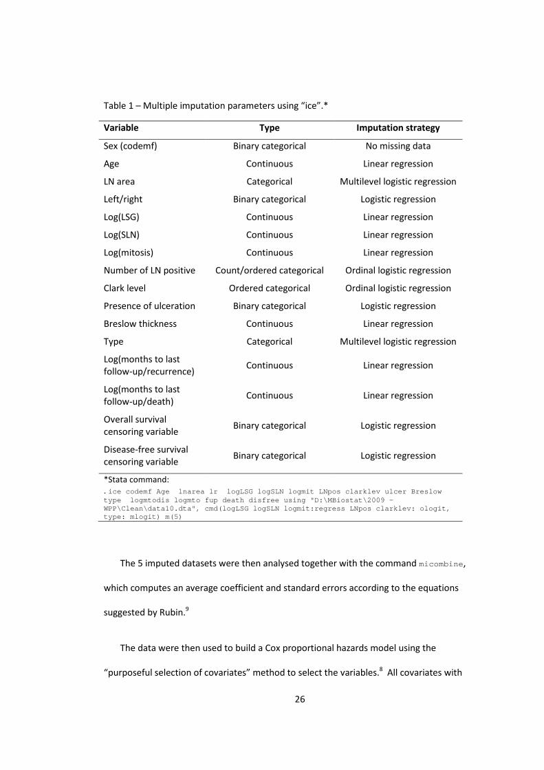
of the settings for the imputation command are shown in Table 1.

26

Table 1 – Multiple imputation parameters using “ice”.*

Variable Type Imputation strategy

Sex (codemf) Binary categorical No missing data

Age Continuous Linear regression

LN area Categorical Multilevel logistic regression

Left/right Binary categorical Logistic regression

Log(LSG) Continuous Linear regression

Log(SLN) Continuous Linear regression

Log(mitosis) Continuous Linear regression

Number of LN positive Count/ordered categorical Ordinal logistic regression

Clark level Ordered categorical Ordinal logistic regression

Presence of ulceration Binary categorical Logistic regression

Breslow thickness Continuous Linear regression

Type Categorical Multilevel logistic regression

Log(months to last follow-up/recurrence) Continuous Linear regression

Log(months to last follow-up/death) Continuous Linear regression

Overall survival censoring variable Binary categorical Logistic regression

Disease-free survival censoring variable Binary categorical Logistic regression

*Stata command: . ice codemf Age lnarea lr logLSG logSLN logmit LNpos clarklev ulcer Breslow type logmtodis logmto fup death disfree using "D:\MBiostat\2009 - WPP\Clean\data10.dta", cmd(logLSG logSLN logmit:regress LNpos clarklev: ologit, type: mlogit) m(5)

The 5 imputed datasets were then analysed together with the command micombine,

which computes an average coefficient and standard errors according to the equations

suggested by Rubin.9

The data were then used to build a Cox proportional hazards model using the

“purposeful selection of covariates” method to select the variables.8 All covariates with

27

P<0.25 on univariate analysis were selected for the initial multivariate model, along with

those covariates considered important in answering our research question. The least

significant terms were progressively removed from this model. Variables were retained in

the final multivariate model if P<0.05 or they were confounding the effect of other

variables on the outcome.

First degree interactions were added to the final reduced model to investigate the

presence of effect modification.

The final model was then assessed for:

• presence of appropriate form for continuous variables, by assessing the

linearity of the Martingale residuals of a model excluding the covariate of

interest;

• validity of the assumption of proportional hazards using Shoenfeld residuals;

• Goodness-of-fit using Cox-Snell residuals.

Note that Stata does not allow the performance of model diagnostics across all five

imputed datasets, so the above were only performed on the first imputed dataset. Due to

this, it is expected that the residuals calculated would be higher than expected, as the final

model is based upon the combined estimate from the models of each imputed dataset

rather than on the particular dataset used for residual analysis.

28

Results

Description of subjects 3127 patients were initially identified in the database. Of these, 14 patients were

identified on final pathology to have either a blue naevus or melanoma in-situ. These

ineligible patients were excluded, leaving 3113 patients for analysis. The median follow-up

time for these subjects was 46.5 months.

Data cleaning resulted in the following adjustments:

• 12 corrected ages

• 1 patient with Clark level “6” (does not exist) was changed to level “5”

• 1 patient where the recurrence date was later than the last follow-up date –

the last follow-up date was therefore adjusted to be equal to the date of

recurrence.

• 17 tumour types were incorrectly typed in (eg, entered in the datsheet as SM

rather than SSM for superficial spreading melanoma).

Patient characteristics are summarised in Table 2. Of note is that there is a

predominance of males. Most common lymph node basin is in the axilla and the upper

limb nodal basins. The median number of nodes detected at LSG and removed at sentinel

node surgery was the same (2 (IQR 1-3)) but the actual range was much greater for the

latter (1-9 vs 1-31). The consequent lymph node yield at surgery varied from 0.25 to 15.

The Clark levels and Breslow thicknesses found in the specimen reflect a predominance

of intermediate thickness melanoma in our patient population which is the group in which

sentinel node surgery is most beneficial.

29

Table 2 – Summary of patient characteristics and the number of missing data for each variable. Number of

observations Number missing (%)

Demographic characteristics Male/female 3113 0 (0%) Female 1224

Male 1889

Age 3111 2 (0%) Mean 56.3 (SD 15.8)

Follow-up 2953 160 (5.1%) Median 46.5 (IQR 24.1-71.2) Lymph node characteristics LN areas 2965 148 (4.8%) Axilla/upper limb 1365

Groin/lower limb 886 Neck/axial 492 Multiple 202

Left/right 2963 150 (4.8%) Left 1359 Right 1368 Bilateral 236

Number of nodes on LSG

2961 152 (4.9%) Median 2 (IQR 1-3) nodes

Number of nodes at surgery

3110 3 (0%) Median 2 (IQR 1-3) nodes

LN positive for cancer 3110 3 (0%) 0 (0-0) nodes Characteristics of primary cancer Mitoses/mm2 3069 44 (1.4%) Median 3 (IQR 1-6)

Clark level 3027 86 (2.8%) level 1 4

level 2 97 level 3 776 level 4 1912 level 5 238

Presence of ulceration 3070 43 (1.4%) non-ulcerated 2337 ulcerated 733

Breslow thickness (mm) 3075 38 (1.2%) Mean 2.43 (SD 1.85)

Tumour type 2540 573 (18.4%)

SSM 1048 NM 1145 AL 56 LMM 48 Desmoplastic 243

Abbreviations: AL = Acral lentiginous melanoma; IQR = interquartile range; LMM = Lentigo maligna melanoma; LN = Lymph node; LSG = Lymphoscintigraphy; NM = nodular melanoma; SSM = Superficial spreading melanoma

30

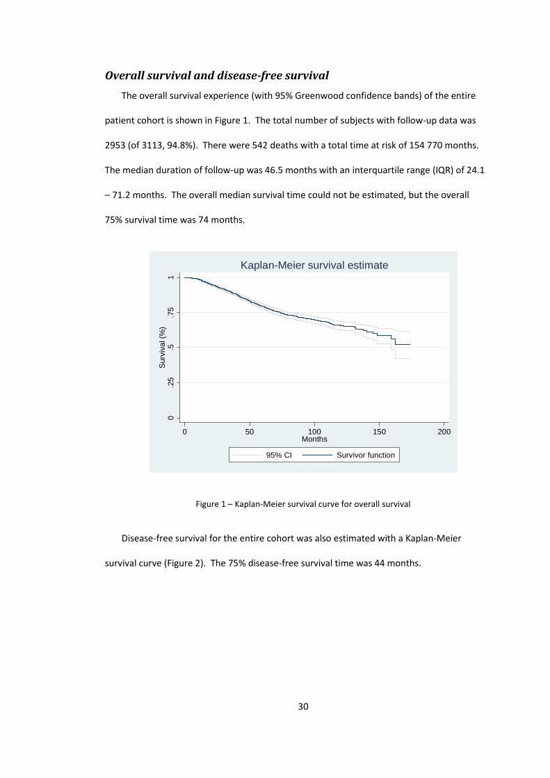
Overall survival and disease-free survival The overall survival experience (with 95% Greenwood confidence bands) of the entire

patient cohort is shown in Figure 1. The total number of subjects with follow-up data was

2953 (of 3113, 94.8%). There were 542 deaths with a total time at risk of 154 770 months.

The median duration of follow-up was 46.5 months with an interquartile range (IQR) of 24.1

– 71.2 months. The overall median survival time could not be estimated, but the overall

75% survival time was 74 months.

0.2

5.5

.75

1Su

rviv

al (%

)

0 50 100 150 200Months

95% CI Survivor function

Kaplan-Meier survival estimate

Figure 1 – Kaplan-Meier survival curve for overall survival

Disease-free survival for the entire cohort was also estimated with a Kaplan-Meier

survival curve (Figure 2). The 75% disease-free survival time was 44 months.

31

0.2

5.5

.75

1D

isea

se fr

ee s

urvi

val

0 50 100 150 200Months

95% CI Survivor function

Kaplan-Meier survival estimate

Figure 2 – Kaplan-Meier survival curve for disease-free survival

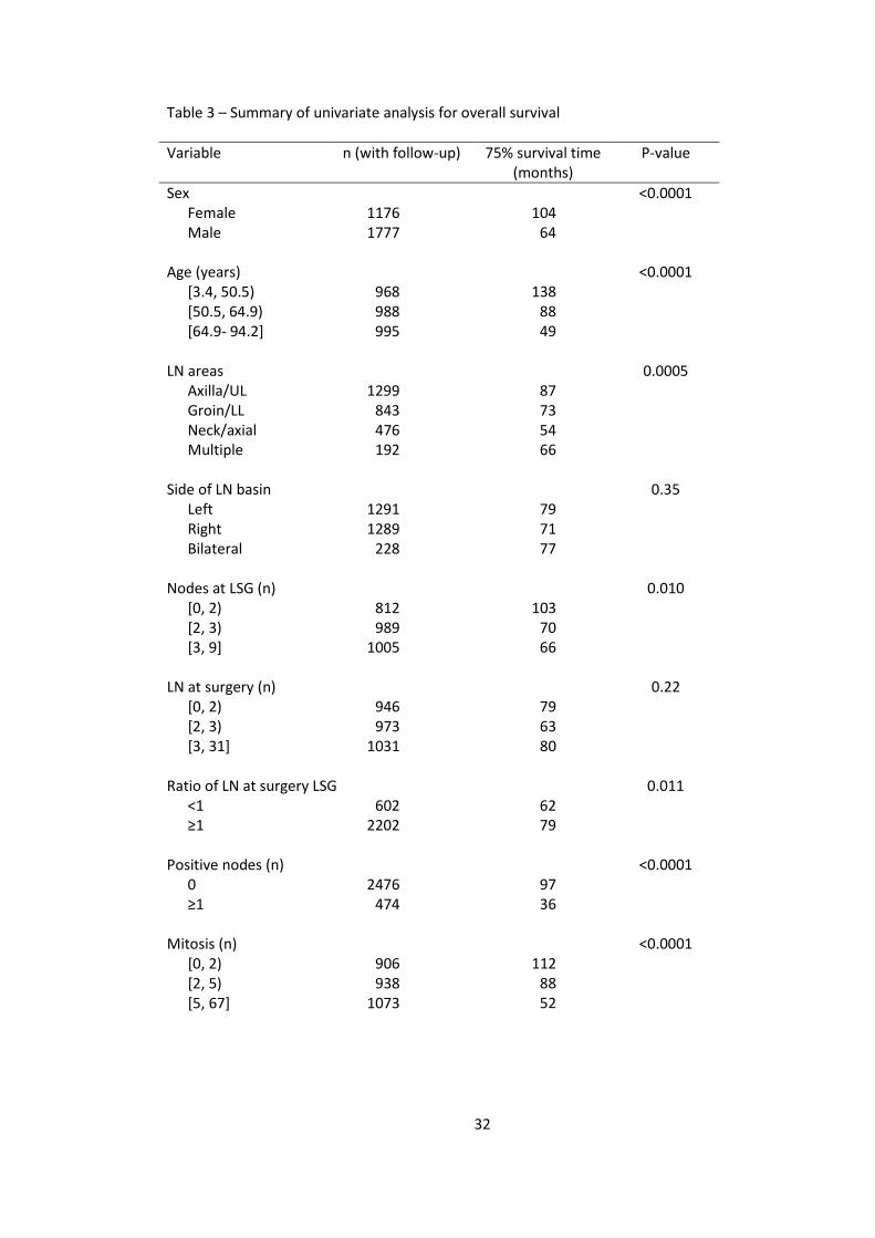
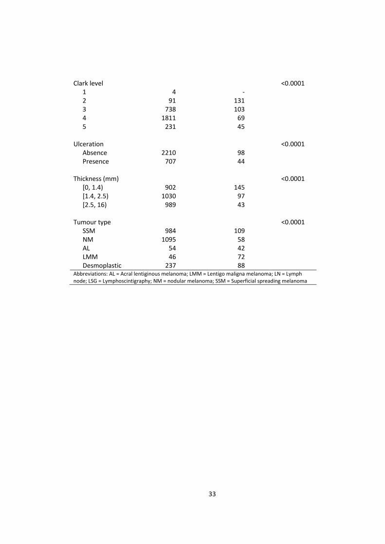
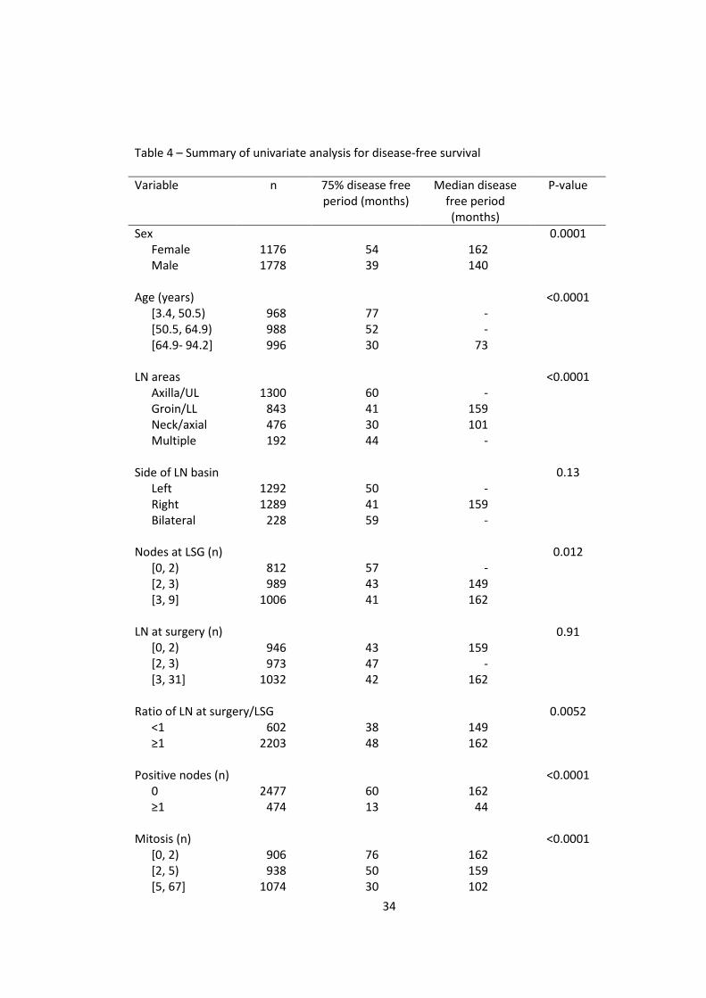
The results of univariate analysis and the cut-points used for categorisation are shown

in the following table (Table 3). Note that the left square bracket means that the value is

included and right round bracket means it is not included in range.

In addition to the known factors associated with poor outcome (male sex, old age,

presence of ulceration, thickness of tumour, positive lymph nodes), the number of nodes

found at initial lymphoscintigraphy and the subsequent yield of lymph nodes at surgery

were also found to be predictive factors of survival on univariate analysis. The same factors

that significantly affected overall survival also affected disease-free survival significantly.

32

Table 3 – Summary of univariate analysis for overall survival Variable n (with follow-up) 75% survival time

(months) P-value

Sex Female Male

1176 1777

104 64

<0.0001

Age (years) [3.4, 50.5) [50.5, 64.9) [64.9- 94.2]

968 988 995

138 88 49

<0.0001

LN areas Axilla/UL Groin/LL Neck/axial Multiple

1299 843 476 192

87 73 54 66

0.0005

Side of LN basin Left Right Bilateral

1291 1289 228

79 71 77

0.35

Nodes at LSG (n) [0, 2) [2, 3) [3, 9]

812 989 1005

103 70 66

0.010

LN at surgery (n) [0, 2) [2, 3) [3, 31]

946 973 1031

79 63 80

0.22

Ratio of LN at surgery LSG

0.011

<1 ≥1

602 2202

62 79

Positive nodes (n) 0 ≥1

2476 474

97 36

<0.0001

Mitosis (n) [0, 2) [2, 5) [5, 67]

906 938 1073

112 88 52

<0.0001

33

Clark level 1 2 3 4 5

4 91 738 1811 231

- 131 103 69 45

<0.0001

Ulceration Absence Presence

2210 707

98 44

<0.0001

Thickness (mm) [0, 1.4) [1.4, 2.5) [2.5, 16)

902 1030 989

145 97 43

<0.0001

Tumour type SSM NM AL LMM Desmoplastic

984 1095 54 46 237

109 58 42 72 88

<0.0001

Abbreviations: AL = Acral lentiginous melanoma; LMM = Lentigo maligna melanoma; LN = Lymph node; LSG = Lymphoscintigraphy; NM = nodular melanoma; SSM = Superficial spreading melanoma

34

Table 4 – Summary of univariate analysis for disease-free survival Variable n 75% disease free

period (months) Median disease

free period (months)

P-value

Sex Female Male

1176 1778

54 39

162 140

0.0001

Age (years) [3.4, 50.5) [50.5, 64.9) [64.9- 94.2]

968 988 996

77 52 30

- - 73

<0.0001

LN areas Axilla/UL Groin/LL Neck/axial Multiple

1300 843 476 192

60 41 30 44

- 159 101 -

<0.0001

Side of LN basin Left Right Bilateral

1292 1289 228

50 41 59

- 159 -

0.13

Nodes at LSG (n) [0, 2) [2, 3) [3, 9]

812 989 1006

57 43 41

- 149 162

0.012

LN at surgery (n) [0, 2) [2, 3) [3, 31]

946 973 1032

43 47 42

159 - 162

0.91

Ratio of LN at surgery/LSG

0.0052

<1 ≥1

602 2203

38 48

149 162

Positive nodes (n) 0 ≥1

2477 474

60 13

162 44

<0.0001

Mitosis (n) [0, 2) [2, 5) [5, 67]

906 938 1074

76 50 30

162 159 102

<0.0001

35

Clark level 1 2 3 4 5

4 91 739 1811 231

- 52 65 42 19

- 131 - 159 71

<0.0001

Ulceration Absence Presence

2210 708

58 20

167 70.9

<0.0001

Thickness (mm) [0, 1.4) [1.4, 2.5) [2.5, 16)

902 1030 990

126 51 23

- 162 70.9

<0.0001

Tumour type SSM NM AL LMM Desmoplastic

984 1096 54 46 237

73 33 13 40 51

- 105 47 131 -

<0.0001

Abbreviations: AL = Acral lentiginous melanoma; LMM = Lentigo maligna melanoma; LN = Lymph node; LSG = Lymphoscintigraphy; NM = nodular melanoma; SSM = Superficial spreading melanoma

36

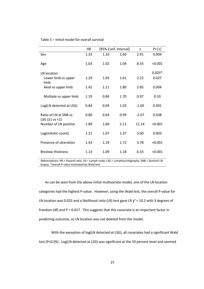
Multivariate modelling of overall survival After performing multiple imputation, a multivariate proportional hazards model was

fitted. The initial model for overall survival included the following covariates: sex, age,

lymph node basin, nodes found at lymphoscintigraphy, nodes extracted at surgery, whether

lymph node yield was 100% or greater (primary outcome of interest), number of positive

nodes, number of mitosis, presence of ulceration and tumour thickness. Using the criterion

of P<0.25 on univariate analysis, all but “side of LN basin” were eligible to be included.

However, the following covariates were not included in the initial multivariate model:

• logSLN as this is a figure which is unknown at time of surgery. Also, by knowing

LSG and the ratio, logSLN can be defined. Therefore there is duplication of

information if it is included.

• Clark levels and tumour types were not included in the initial model despite

having a significant effect on outcome on univariate analysis because it is well

known clinically that these factors affect patient outcome through the

influence of tumour thickness. These two covariates if included will complicate

the modelling as each of them is a multilevel categorical variable, with Clark

levels being ordered. In addition, both have at least 2 categories with very few

patients.

The initial model is shown in Table 5.

37

Table 5 – Initial model for overall survival HR [95% Conf. Interval] z P>|z| Sex

1.33 1.10 1.60 2.91 0.004

Age

1.03 1.02 1.04 8.55 <0.001

LN location 0.025* Lower limb vs upper limb

1.29 1.03 1.61 2.22 0.027

Axial vs upper limb

1.42 1.11 1.80 2.85 0.004

Multiple vs upper limb

1.19 0.84 1.70 0.97 0.33

Log(LN detected at LSG)

0.84 0.69 1.03 -1.69 0.091

Ratio of LN at SNB vs LSG (≥1 vs <1)

0.80 0.64 0.99 -2.07 0.038

Number of LN positive

1.89 1.69 2.12 11.14 <0.001

Log(mitotic count)

1.21 1.07 1.37 3.00 0.003

Presence of ulceration

1.43 1.19 1.72 3.78 <0.001

Breslow thickness

1.13 1.09 1.18 6.33 <0.001

Abbreviations: HR = Hazard ratio; LN = Lymph node; LSG = Lymphoscintigraphy; SNB = Sentinel LN biopsy. *overall P-value estimated by Wald test

As can be seen from the above initial multivariate model, one of the LN location

categories had the highest P-value. However, using the Wald test, the overall P-value for

LN location was 0.025 and a likelihood ratio (LR) test gave LR χ² = 10.2 with 3 degrees of

freedom (df) and P = 0.017. This suggests that this covariate is an important factor in

predicting outcome, so LN location was not deleted from the model.

With the exception of log(LN detected at LSG), all covariates had a significant Wald

test (P<0.05). Log(LN detected at LSG) was significant at the 10 percent level and seemed

38

to be a relatively important clinical variable, so we checked its importance by refitting a

model without it. The resulting model is shown in table 6.

Table 6 – Comparison of models with and without log(LN detected at LSG) Coeff P>|z| Coeff P>|z| Sex

0.28 0.004 0.27 0.005

Age

0.03 <0.001 0.03 <0.001

LN location 0.025* 0.065*

Lower limb vs upper limb

0.25 0.027 0.20 0.071

Axial vs upper limb

0.35 0.004 0.31 0.011

Multiple vs upper limb

0.18 0.33 0.10 0.59

Log(LN detected at LSG)

-0.17 0.091 - -

Ratio of LN at SNB vs LSG (≥1 vs <1)

-0.23 0.038 -0.15 0.14

Number of LN positive

0.64 <0.001 0.62 <0.001

Log(mitotic count)

0.19 0.003 0.19 0.002

Presence of ulceration

0.36 <0.001 0.36 <0.001

Breslow thickness

0.12 <0.001 0.12 <0.001

Abbreviations: Coeff = log(HR); HR = Hazard ratio; LN = Lymph node; LSG = Lymphoscintigraphy; SNB = Sentinel LN biopsy. *overall P-value estimated by Wald test

The coefficients for most variables above demonstrate minimal change, but the

coefficients for variables describing LN location and the coefficient for LN ratio have

changed markedly (>20%). This suggests that log(LN detected at LSG) is an important

confounding factor. The LR test (LR χ² = 3.08; 1 df) gave P = 0.079. The above therefore

suggests that log(LN detected at LSG) is an important covariate which should not be

removed from the final model.

39

At this point, no further variable can be deleted. First-order interactions between LN

ratio and other covariates were found not to be significant. Therefore the above formed

the final model.

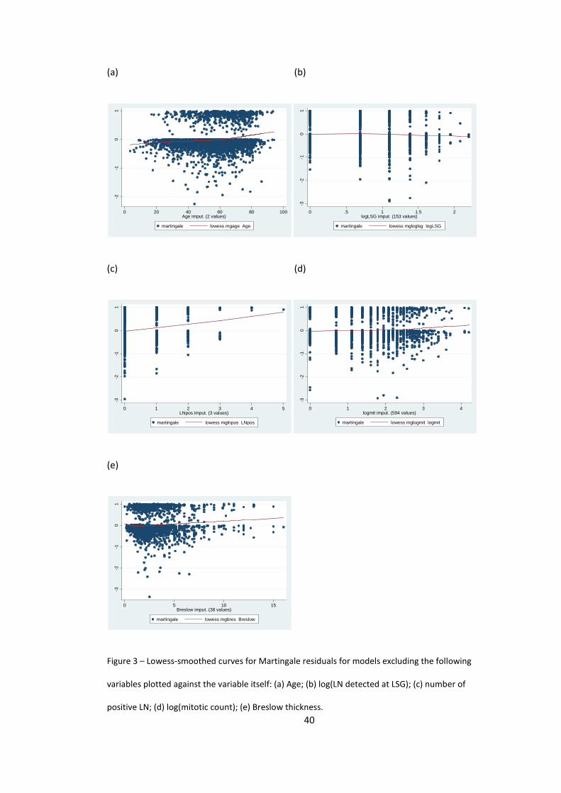
Model diagnostics (for overall survival model) The functional form of the continuous covariates was checked by plotting the

Martingale residuals against the covariate of interest after fitting the Cox model without

that covariate.

40

(a) (b)

-2-1

01

0 20 40 60 80 100Age imput. (2 values)

martingale lowess mgage Age

-3-2

-10

1

0 .5 1 1.5 2logLSG imput. (153 values)

martingale lowess mgloglsg logLSG

(c) (d)

-3-2

-10

1

0 1 2 3 4 5LNpos imput. (3 values)

martingale lowess mglnpos LNpos

-3-2

-10

1

0 1 2 3 4logmit imput. (594 values)

martingale lowess mglogmit logmit

(e)

-3-2

-10

1

0 5 10 15Breslow imput. (38 values)

martingale lowess mgbres Breslow

Figure 3 – Lowess-smoothed curves for Martingale residuals for models excluding the following

variables plotted against the variable itself: (a) Age; (b) log(LN detected at LSG); (c) number of

positive LN; (d) log(mitotic count); (e) Breslow thickness.

41

The plots for the continuous variables, age, log(LN detected at LSG), number of positive

LN, log(mitotic count) and Breslow thickness all demonstrated a close to linear Lowess

smoothed curve for the Martingale residuals (figure 3). This suggests that the covariates

are in an appropriate form and do not require transformation.

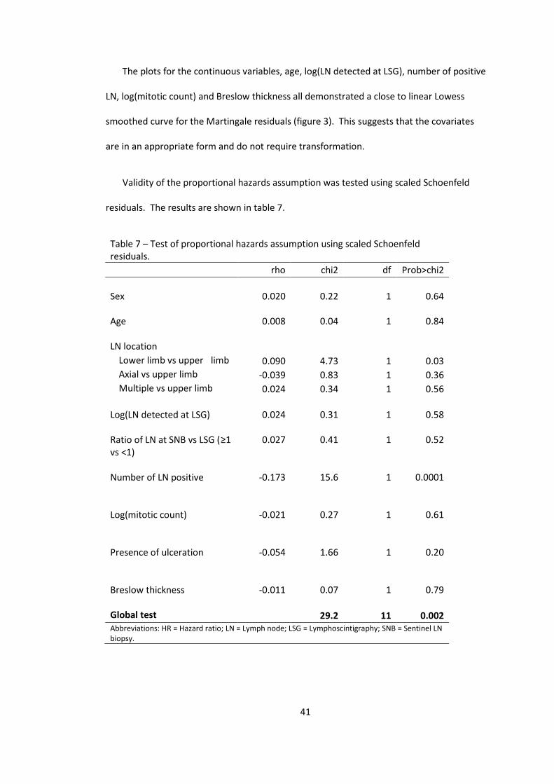
Validity of the proportional hazards assumption was tested using scaled Schoenfeld

residuals. The results are shown in table 7.

Table 7 – Test of proportional hazards assumption using scaled Schoenfeld residuals. rho chi2 df Prob>chi2 Sex

0.020

0.22

1

0.64

Age

0.008 0.04 1 0.84

LN location Lower limb vs upper limb 0.090 4.73 1 0.03 Axial vs upper limb -0.039 0.83 1 0.36 Multiple vs upper limb 0.024 0.34 1 0.56 Log(LN detected at LSG)

0.024

0.31

1

0.58

Ratio of LN at SNB vs LSG (≥1 vs <1)

0.027 0.41 1 0.52

Number of LN positive

-0.173 15.6 1 0.0001

Log(mitotic count)

-0.021 0.27 1 0.61

Presence of ulceration

-0.054 1.66 1 0.20

Breslow thickness

-0.011 0.07 1 0.79

Global test 29.2 11 0.002 Abbreviations: HR = Hazard ratio; LN = Lymph node; LSG = Lymphoscintigraphy; SNB = Sentinel LN biopsy.

42

The above demonstrates that the proportional hazards assumption of the model has

been violated. This appears to be mainly due to “number of positive LN” (P=0.0001) but

also to the indicator variable for lower limb vs upper limb LN location (P =0.03).

The model was therefore refitted after stratifying for location of lymph nodes and the

number of positive LN. Note however that the distribution of the number of positive lymph

nodes, shown in figure 4, suggests that while it is in theory a continuous variable, in fact the

vast majority of patients had a value of 0 and very few had values greater than 1.

050

001.

0e+0

41.

5e+0

4Fr

eque

ncy

0 1 2 3 4 5No of positive LN (5 imputation sets)

Figure 4 – Histogram demonstrating the distribution of the number of positive lymph nodes found in

patients in the study (note that this is a histogram of 5 imputation datasets, therefore, the total

number of observations is 15565).

Therefore, I decided to convert this into an indicator variable with 1 indicating the

presence of positive lymph nodes and use this binary categorical variable to stratify the

data. However, before stratifying the data, the new binary variable was used to refit the

model and it was confirmed that this new model still violates the proportional hazards

assumption.

43

After stratifying for lymph node location and the presence of positive lymph nodes at

SLNB, the resulting model is shown in table 8.

Table 8 – Stratified final model for overall survival HR [95% Conf. Interval] z P>|z| Sex

1.35 1.11 1.63 3.08 0.002

Age

1.03 1.02 1.03 8.02 <0.001

Ratio of LN at SNB vs LSG (≥1 vs <1)

0.88 0.72 1.08 1.25 0.21

Log(mitotic count)

1.21 1.07 1.37 3.06 0.002

Presence of ulceration

1.42 1.18 1.71 3.76 <0.001

Breslow thickness

1.13 1.08 1.17 6 <0.001

Abbreviations: HR = Hazard ratio; LN = Lymph node; SNB = Sentinel LN biopsy.

The baseline survival curves for the 8 strata are shown in figure 5. As can be seen, LN

positive and LN negative curves are quite different from each other. Also, in the LN positive

group, different lymph node location groups have different survival curves as well. This is

reassuring as it justifies our decision to stratify the data.

44

.9.9

51

0 50 100 150 200_t

LN neg + upper limb LN neg + lower limbLN neg + axial LN neg + multiple sitesLN pos + upper limb LN pos + lower limbLN pos + axial LN pos + multiple sites

Figure 5 – “Baseline” survival curves for the 8 strata in the final model.

The proportional hazards assumption was tested again using scaled Schoenfeld

residuals. This stratified model no longer violates this assumption.

Table 9 – Test of proportional hazards assumption of stratified model using scaled Schoenfeld residuals. rho chi2 df Prob>chi2 Sex

0.013 0.09 1 0.76

Age

0.030 0.57 1 0.45

Ratio of LN at SNB vs LSG (≥1 vs <1)

-0.012 0.08 1 0.78

Log(mitotic count)

-0.024 0.34 1 0.56

Presence of ulceration

-0.047 1.22 1 0.27

Breslow thickness

-0.015 0.11 1 0.74

Global test 2.94 6 0.82 Abbreviations: HR = Hazard ratio; LN = Lymph node; LSG = Lymphoscintigraphy; SNB = Sentinel LN biopsy.

Overall goodness of fit of the model with Cox-Snell residuals gives the following plot.

45

01

23

0 1 2 3Cox-Snell residual

Nelson-Aalen cumulative hazard Cox-Snell residual

Figure 6 – Cumulative hazard function with Cox-Snell residuals as failure times to test goodness-of-fit

of the model.

This indicates that for the vast majority of observations, the goodness of fit of the

model is high. Only 4 observations out of 3113 appear not to be fit by the model quite so

well.

46

Multivariate modelling of disease-free survival The covariates of the initial model (Table 10) were the same as for the initial overall

survival model.

Table 10 – Initial model for disease-free survival HR [95% Conf. Interval] z P>|z| Sex

1.20 1.03 1.40 2.33 0.02

Age

1.02 1.02 1.03 9.26 <0.001

LN location 0.0038* Lower limb vs upper limb

1.29 1.08 1.53 2.83 0.005

Axial vs upper limb

1.33 1.10 1.60 2.93 0.003

Multiple vs upper limb

1.04 0.78 1.39 0.28 0.779

Log(LN detected at LSG)

0.94 0.80 1.09 -0.84 0.402

Ratio of LN at SNB vs LSG (≥1 vs <1)

0.84 0.71 1.00 -1.94 0.053

Number of LN positive

1.79 1.62 1.97 11.5 <0.001

Log(mitotic count)

1.18 1.08 1.29 3.7 <0.001

Presence of ulceration

1.34 1.15 1.55 3.79 <0.001

Breslow thickness

1.12 1.09 1.16 7.06 <0.001

Abbreviations: HR = Hazard ratio; LN = Lymph node; LSG = Lymphoscintigraphy; SNB = Sentinel LN biopsy. *overall P-value estimated by Wald test

The model was reduced by in turn removing the log(LN detected at LSG), as shown in

table 11.

47

Table 11 – Reduced model for disease-free survival HR [95% Conf. Interval] Z P>|z| Sex

1.20 1.03 1.40 2.29 0.022

Age

1.02 1.02 1.03 9.24 <0.001

LN location 0.0053* Lower limb vs upper limb

1.26 1.07 1.49 2.7 0.007

Axial vs upper limb

1.30 1.08 1.57 2.82 0.005

Multiple vs upper limb

1.01 0.76 1.34 0.07 0.94

Ratio of LN at SNB vs LSG (≥1 vs <1)

0.87 0.74 1.02 -1.75 0.081

Number of LN positive

1.77 1.61 1.95 11.55 <0.001

Log(mitotic count)

1.19 1.08 1.30 3.75 <0.001

Presence of ulceration

1.34 1.15 1.56 3.8 <0.001

Breslow thickness

1.12 1.09 1.16 7.01 <0.001

Abbreviations: HR = Hazard ratio; LN = Lymph node; LSG = Lymphoscintigraphy; SNB = Sentinel LN biopsy. *overall P-value estimated by Wald test

In this model, the largest P-value is 0.081 for LN ratio. As this is the variable of interest

of the study it was kept in the model. No further reduction in this model is possible. First-

order interactions of LN ratio with other covariates were not significant, so this model

forms the final model.

Model diagnostics for the disease-free survival model The functional form of the continuous covariates was checked in the same way as for

the overall survival model. The plots for age, number of positive LN, log(mitotic count) and

Breslow thickness all demonstrated a close to linear Lowess smoothed curve suggesting

that the covariates are in an appropriate form and do not require transformation (figure 7).

48

(a) (b)

-3-2

-10

1

0 20 40 60 80 100Age imput. (2 values)

martingale lowess mgage2 Age

-3-2

-10

1

0 1 2 3 4 5LNpos imput. (3 values)

martingale lowess mglnpos2 LNpos

(c) (d)

-4-3

-2-1

01

0 1 2 3 4logmit imput. (594 values)

martingale lowess mglogmit2 logmit

-3-2

-10

1

0 5 10 15Breslow imput. (38 values)

martingale lowess mgbreslow2 Breslow

Figure 7 – Lowess-smoothed curves for Martingale residuals for models excluding the following

variables plotted against the variable itself: (a) Age; (b) number of positive LN; (c) log(mitotic count);

(d) Breslow thickness.

Using Schoenfeld residuals, the proportional hazards assumption was tested (Table 12).

Age, presence of ulceration, and number of lymph nodes positive were found to have

violated this assumption.

49

Table 12 – Test of proportional hazards assumption with Schoenfeld residuals.

rho chi2 df Prob>chi2 Sex

0.012 0.1 1 0.720

Age

0.068 4.9 1 0.026

LN location Lower limb vs upper limb

0.018 0.3 1 0.594

Axial vs upper limb

-0.060 3.2 1 0.074

Multiple vs upper limb

-0.042 1.6 1 0.21

Ratio of LN at SNB vs LSG (≥1 vs <1)

0.016 0.2 1 0.63

Number of LN positive

-0.149 18.0 1 <0.0001

Log(mitotic count)

-0.030 0.9 1 0.348

Presence of ulceration

-0.104 9.6 1 0.002

Breslow thickness

-0.009 0.1 1 0.797

Global test 49.28 10 <0.0001 Abbreviations: HR = Hazard ratio; LN = Lymph node; LSG = Lymphoscintigraphy; SNB = Sentinel LN biopsy. *overall P-value estimated by Wald test

The model was therefore stratified according to the above variables. The number of

lymph node positive was categorised as for the analysis of overall survival. Age was also

categorised into the 3 categories used in univariate analysis (table 3). This new model with

12 strata is shown in table 13.

50

Table 13 – Stratified model for disease-free survival HR [95% Conf. Interval] Z P>|z| Sex

1.22 1.05 1.43 2.53 0.011

LN location 0.0076* Lower limb vs upper limb

1.24 1.05 1.47 2.53 0.011

Axial vs upper limb

1.32 1.09 1.58 2.9 0.004

Multiple vs upper limb

1.04 0.78 1.38 0.25 0.805

Ratio of LN at SNB vs LSG (≥1 vs <1)

0.90 0.76 1.05 -1.38 0.17

Log(mitotic count)

1.18 1.08 1.30 3.71 <0.001

Breslow thickness

1.12 1.08 1.16 6.83 <0.001

Abbreviations: HR = Hazard ratio; LN = Lymph node; LSG = Lymphoscintigraphy; SNB = Sentinel LN biopsy. *overall P-value estimated by Wald test

Rechecking the proportional hazards assumption gives table 14. This demonstrates

that whilst two LN location dummy variables were almost significant for violation of the

proportional hazards assumption, neither was. The global test also was non-significant

(P=0.24). We also investigated the possibility of refitting the model with LN location

stratified, but found that the coefficients and P-values of the remaining variables were

minimally changed but the model had 3 times the number of strata of the existing model

(ie, 36 strata). Therefore, by the principle of parsimony, we decided not to further stratify

the model.

51

Table 14 – Proportional hazards assumption tested for the final stratified model for disease-free survival

rho chi2 df Prob>chi2 Sex

0.007 0.04 1 0.84

LN location Lower limb vs upper limb

0.011 0.12 1 0.73

Axial vs upper limb

-0.062 3.36 1 0.07

Multiple vs upper limb

-0.063 3.56 1 0.06

Ratio of LN at SNB vs LSG (≥1 vs <1)

0.014 0.18 1 0.67

Log(mitotic count)

-0.022 0. 48 1 0.49

Breslow thickness

-0.002 0.00 1 0.96

Global test 9.19 7 0.24 Abbreviations: HR = Hazard ratio; LN = Lymph node; LSG = Lymphoscintigraphy; SNB = Sentinel LN biopsy. *overall P-value estimated by Wald test

Overall goodness of fit of the model with Cox-Snell residuals gives the following plot.

01

23

0 .5 1 1.5 2 2.5Cox-Snell residual

Nelson-Aalen cumulative hazard Cox-Snell residual

Figure 8 - Cumulative hazard function with Cox-Snell residuals as failure times to test goodness-

of-fit of the model for disease-free survival.

52

Again, like the overall survival model, the goodness-of-fit is high for the vast majority of

the observations (except for one out of 3113).

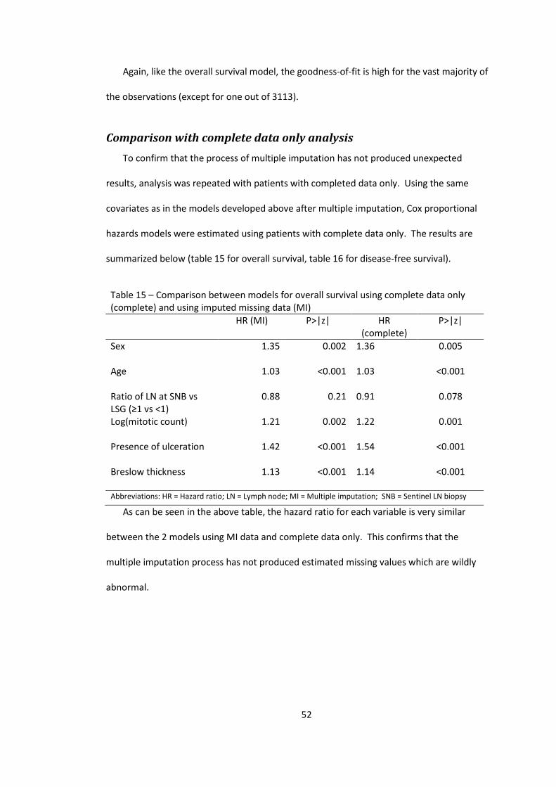
Comparison with complete data only analysis To confirm that the process of multiple imputation has not produced unexpected

results, analysis was repeated with patients with completed data only. Using the same

covariates as in the models developed above after multiple imputation, Cox proportional

hazards models were estimated using patients with complete data only. The results are

summarized below (table 15 for overall survival, table 16 for disease-free survival).

Table 15 – Comparison between models for overall survival using complete data only (complete) and using imputed missing data (MI)

HR (MI) P>|z| HR

(complete) P>|z|

Sex

1.35 0.002 1.36 0.005

Age

1.03 <0.001 1.03 <0.001

Ratio of LN at SNB vs LSG (≥1 vs <1)

0.88 0.21 0.91 0.078

Log(mitotic count)

1.21 0.002 1.22 0.001

Presence of ulceration

1.42 <0.001 1.54 <0.001

Breslow thickness

1.13 <0.001 1.14 <0.001

Abbreviations: HR = Hazard ratio; LN = Lymph node; MI = Multiple imputation; SNB = Sentinel LN biopsy As can be seen in the above table, the hazard ratio for each variable is very similar

between the 2 models using MI data and complete data only. This confirms that the

multiple imputation process has not produced estimated missing values which are wildly

abnormal.

53

Table 16 – Comparison between models using complete data only (complete) and using imputed missing data (MI) for disease-free survival

HR (MI) P>|z| HR

(complete) P>|z|

Sex

1.22 0.011 1.16 0.09

LN location 0.0076* 0.012* Lower limb vs upper limb

1.24 0.011 1.30 0.006

Axial vs upper limb

1.32 0.004 1.32 0.010

Multiple vs upper limb

1.04 0.805 1.03 0.865

Ratio of LN at SNB vs LSG (≥1 vs <1)

0.90 0.168 0.96 0.433

Log(mitotic count)

1.18 <0.001 1.23 <0.001

Breslow thickness

1.12 <0.001 1.14 <0.001

Abbreviations: HR = Hazard ratio; LN = Lymph node; MI = Multiple imputation; SNB = Sentinel LN biopsy. *Overall P-value estimated by Wald test.

Again, for disease-free survival, the models using the different data are similar,

although less so than for overall survival.

Interpretation of results for a non-statistical audience

Hazard ratio is a way of conceptualizing the risk of “failure” – in this case, it represents

the ratio of the risk of dying at any one time in one group of patients compared to another.

The 95% confidence interval represents the range of hazard ratios that would be found in

95% (ie, 19 of 20) of studies if one were to repeat the study many times. That is, one is 95%

confident that the true hazard ratio lies within the given range.

Overall Survival

The final model for overall survival with hazard ratios, P-values and confidence intervals

is shown in table 8. Note that this model is stratified according to the presence of positive

54

LN and the location of the sentinel LN. That is, the following results can only be interpreted

by comparing patients with the same combination of the above two factors.

According to this final model, we found that:

• Male sex is associated with a 35% higher risk of death than females. Had we

repeated the study 20 times, the increased risk will be found to be between 11%

and 63% greater in men than women in 19 studies, on average.

• There is an increasing risk with increasing age. For 2 people with an age difference

of 1 year, the risk is 3% higher for the older person. This will be found to be

between 2-3% in 95% of times.

o The hazard ratio for a 10-year age difference can also be calculated by:

HR10y = exp(10b1y) = exp(0.272) = 1.31

o Therefore, in 2 people with an age difference of 10 years, the risk of death

in the older person is 31% greater than that of the younger person.

Similarly, the 95% confidence interval can be worked out to be 23% to

40%.

• The presence of ulceration is also an important factor, those patients with

ulceration having a 42% higher risk of death at any time. We are 95% confident

that this lies between 18 and 71%.

• The thicker the tumour, the higher the risk of death. For each 1mm increase in

thickness, the risk of death is increased by 13%. We are 95% confident that the

increase in the risk of death is between 8 and 17% for each 1mm increase in depth.

• In relation to the number of mitoses found at histology, for each logarithmic unit

difference increase of mitoses, the risk of death increases by 21%. That is, for each

2.7 times increase in the number of mitoses detected on histopathology, the risk of

55

death increases by 21%. We can be 95% certain that this is between 7% and 37%

increase in risk with increasing mitotic count.

• Finally, in relation to the outcome of interest, the lymph node yield was not found

to have a statistically significant effect on survival. The P-value was 0.21, which

means that there is a 21% chance that the observed magnitude of change could

have occurred purely by chance alone. This is greater than our preset upper limit

of 5% which we consider statistically significant. In the currently sampled patients,

it seems that the presence of a high lymph node yield (>1) at surgery will lead to a

12% decrease of the risk of death. However if we repeated this study many times,

95% of times we will get a result that ranges from improving the risk of death by

28% to increasing the risk of death by 8% (95% CI 0.72-1.08%).

We therefore cannot conclude that a high lymph node yield at surgery (LN at SNB/LN at

LSG>1) is associated with improved overall survival.

The final model for disease-free survival is detailed in table 13. This model is stratified by

age, lymph node positive status, and presence of ulceration.

Disease-free survival

Therefore, this study shows that:

• Male sex is associated with a 22% higher risk of recurrence or death compared to

females. Had we repeated the study 20 times, the increased risk would have been

found to be between 5% and 43% greater in men than women in 19 times, on

average.

• Compared to patients who have their sentinel nodes found in the upper limb

nodes, those who have sentinel nodes found in the lower limb will have a 24%

higher risk of recurrence/death. If we repeated this study many times, we would

56

find that this increase in risk lies between 5 and 47% in 95% of the times. Sentinel

nodes being found in the neck or torso is also associated with an increased risk of

recurrence or death of 32%. We are 95% confident that this increase in risk is

between 9 and 58%.

• The thicker the tumour, the higher the risk of recurrence or death. For each 1mm

increase in thickness, the risk of recurrence or death is increased by 12%. We are

95% confident that the increase in the risk of recurrence or death is between 8 and

16% for each 1mm increase in depth.

• In relation to the number of mitoses found at histology, for each logarithmic unit

increase in mitoses, the risk of recurrence or death increases by 18%. That is, for

each 2.7 times increase in the number of mitoses detected on histopathology, the

risk of recurrence or death increases by 19%. We can be 95% certain that this is

between 8% and 30% increase in risk with increasing mitotic count.

• Finally, in relation to the outcome of interest, the lymph node yield was not found

to have a statistically significant effect on disease-free survival. The P-value was

0.17, which means that there is a 17% chance that the observed magnitude of

change could have occurred by pure chance alone. This is greater than our preset

upper limit of 5% which we consider statistically significant. However, on average,

the presence of a high lymph node yield (>1) at surgery would lead to a 10% lower

risk of recurrence/death. The 95% confidence interval in this case is between 24%

decrease and 5% increase in risk of the same.

We therefore cannot conclude that a high lymph node yield at surgery (LN at

SNB/LN at LSG>1) is associated with improved disease-free survival.

57

Discussion

Missing data Missing data are almost inevitable in large datasets such as this one. Missing data can

be classified into 3 categories10:

• Missing completely at random (MCAR) – these missing data are thought to

arise completely randomly in that the property of “missingness” does not

relate to any known information in the data but rather to extraneous factors

(such as missing patient weight variable if that is due to malfunction of the

scales on that visit.)

• Missing at random (MAR) – this kind of missing data is the most commonly

assumed kind. Whilst the missing data arise apparently randomly, any

systematic difference between missing values and observed values can be

explained by differences in observed data. For instance, patients with poor

outcomes may be less likely to return for follow-up, so these patients would

have missing follow-up data.

• Not missing at random (NMAR) occurs when it is known that certain data are

missing in a non-random fashion.

It is important to distinguish between these types of missing data as they affect the

analysis.

There are many different ways of dealing with missing data. The most commonly used

way to deal with incomplete data is either to exclude the subjects with missing data from

the analysis or to use the indicator method. The former method may be acceptable if the

data is indeed MCAR, however, it is often impossible to know that this is the case. This

method will also generate unbiased estimates if the missing data are for:

58

• an outcome variable that is measured once in each individual

• a predictor variable that is unrelated to the outcome.

However, even in cases where such a method generates unbiased estimates, analysing the

data this way will lead to a loss of precision and power.10

Another possible method of dealing with missing data is to use an “indicator method”.

In this method, an indicator variable is added as an extra level for each variable with

missing data. The problem with this is that it inevitably causes bias and it also causes a

large number of new variables.11, 12

The best way to deal with missing data is the use of multiple imputation.10 The

principle of this technique is based on the fact that MAR data are related to other variables,

so their distribution can be estimated from the other measured variables. A new set of

data can therefore be generated with the missing data thus estimated. Essentially, the

estimated population distribution of the variables with missing values is re-sampled to

create a new sample. As the imputed data and the actual data come from the same

population distribution, modelling using the new completed dataset would yield non-

biased estimates.

The variance of the estimates however, would be increased compared to modelling of

the complete data. This additional variance from the “resampling” (imputation) process is

minimised by combining the estimates from models of each of the imputed datasets, which

is why multiple is preferable to single imputation.

Important issues that need to be considered in using this technique include:

• The number of imputations required: it is said that 5 imputations is usually

adequate8, 9

59

• Selecting the variables used for analysis – as many variables should be used as

possible, especially the outcome variable as it often carries information about

the missing variable.13

• Non-normally distributed variables – these should be transformed to

approximate normality before imputation.

Limitations of results

Retrospective studies are often limited by the design and the data that are available for

researchers. This is also the case in this study.

Limitations related to study design and data

Being an observational study rather than a randomised controlled trial, there may be

additional confounding factors which may not have been accounted for by the multivariate

model. These unknown factors may lead to bias of the result.

One of the issues in this study is the short follow-up period after sentinel lymph node

biopsy. Whilst the median follow-up was 46.5 months, median survival was not able to be

estimated when calculating the overall survival. Median disease-free survival was just able

to be calculated. However, the natural history of melanoma is that recurrences or even

mortality do occur many years after the primary diagnosis. This may lead to inaccuracies in

estimating median survival as there are few patients with more than 10 years of data.

Another limitation of the data arises from the accuracy of the collected data. In many

cases, clinical databases are maintained by one individual, but the data are input by a

variety of clinical and non-clinical staff. There is great variation in the accuracy of the data

entered into the database depending on who enters the data. This is a potential source of

bias, especially in a multi-clinician, multi-disciplinary institution such as the Sydney

Melanoma Unit. If, for example, different clinicians with interests in different types of

60

melanomas (eg, metastatic or high grade) record data with different quality or

completeness, then this will bias the data. However, this was partly ameliorated by the

fact that consecutive patients were examined, and careful data cleaning was in place to

review any inconsistencies in the data.

Another important limitation to consider is that the study setting in this case is at a

specialist melanoma unit, which may see a different population of melanoma patients than

that encountered in more general surgical/dermatology units. As sentinel node biopsy is

most beneficial in patients who have intermediate thickness melanoma, this may affect the

external applicability of this study.

However, one good point of the current study is that the sample size is relatively large,

which will reduce the probability of making a type 2 error. This is important especially

since we have found that lymph node ratio did not affect patient outcome. Note that this

does not impact on the potential biasing effects of unrecognised confounders.

As this study is retrospective one is unable to determine for certain whether all sentinel

nodes have been removed, so we utilize the lymph node yield as a surrogate for this. A

ratio of more than 1 does not necessarily reflect complete sentinel lymph node excision.

Furthermore, lymphoscintigraphy is imperfect, which may also bias the outcome. The

quality of lymphoscintigraphy is as important in this study as the quality of surgery.

Limitations related to scientific methodology (lymphoscintigraphy)

Whilst multiple imputation was used to estimate missing data, there are limitations to

this technique. The first is the assumption that the missing data are MAR. If there were

data that were NMAR, then the imputed missing values would be biased. Also, imputing

Limitations relating to analysis

61

values of variables with a non-normal distribution may lead to imputation of extreme or

impossible values which again may lead to bias.

Finally, when multiple imputation is used with modelling, it is not clear whether the

values should be imputed before the model-building process or if it should be performed

after. The former may lead to bias by not incorporating into the imputation process what

can only be known after modelling (eg, non-linear functional forms of continuous

covariates) whilst the latter can lead to bias by restricting the model-building process to

observations with complete data.8

In this study, we have attempted to evaluate the effect of multiple imputation by

comparing the resulting analysis with an analysis restricted to complete data only. The

results confirm that multiple imputation has not led to very abnormal results in this study.

The discrepancies seen between the two analyses probably reflect the bias due to

restricting analysis to observations with complete data only.

62

Conclusion Complete extraction of all sentinel lymph nodes identified at preoperative

lymphoscintigraphy was not found to be associated with statistically significant

improvements in overall or disease-free survival.

Other well-known risk factors (male sex, older age, presence of involved nodes,

presence of ulceration, increased Breslow thickness, high mitotic count, and location of

tumour) were once again confirmed to affect outcome.

63

References 1. Australian Health Ethics Committee. When does quality assurance in health care require independent ethical review? National Health and Medical Research Council: Canberra, 2003. 2. Australian Cancer Network Melanoma Guidlines Revision Working Party. Clinical Practice Guidlines for the Management of Melanoma in Australia and New Zealand. . Cancer Council Australia and Australian Cancer Network, Sydney and New Zealand Guidlines Group: Wellington, 2008. 3. Kelley MC, Ollila DW, Morton DL. Lymphatic mapping and sentinel lymphadenectomy for melanoma. Semin Surg Oncol 1998;14(4): 283-290. 4. Chao C, Wong SL, Ross MI, Reintgen DS, Noyes RD, Cerrito PB, Edwards MJ, McMasters KM. Patterns of early recurrence after sentinel lymph node biopsy for melanoma. Am J Surg 2002;184(6): 520-524; discussion 525. 5. Testori A, De Salvo GL, Montesco MC, Trifiro G, Mocellin S, Landi G, Macripo G, Carcoforo P, Ricotti G, Giudice G, Picciotto F, Donner D, Di Filippo F, Soteldo J, Casara D, Schiavon M, Vecchiato A, Pasquali S, Baldini F, Mazzarol G, Rossi CR. Clinical considerations on sentinel node biopsy in melanoma from an Italian multicentric study on 1,313 patients (SOLISM-IMI). Ann Surg Oncol 2009;16(7): 2018-2027. 6. Faries M. Survival and the Sentinel Lymph Node in Melanoma. Ann Surg Oncol 2009. 7. Royston P. Multiple imputation of missing values: update of ice. Stata J 2005;5: 527-536. 8. Hosmer D, Lemeshow S, May S. Applied survival analysis: Regression modeling of time-to-event data (2nd edn). John Wiley & Sons, Inc: New Jersey, 2008. 9. Rubin D. Multiple imputation for nonresponse in Surveys. . Joh Wiley & Sons, Inc.: New York, 1987. 10. Sterne JA, White IR, Carlin JB, Spratt M, Royston P, Kenward MG, Wood AM, Carpenter JR. Multiple imputation for missing data in epidemiological and clinical research: potential and pitfalls. BMJ 2009;338: b2393. 11. Vach W, Blettner M. Biased estimation of the odds ratio in case-control studies due to the use of ad hoc methods of correcting for missing values for confounding variables. Am J Epidemiol 1991;134(8): 895-907. 12. Donders AR, van der Heijden GJ, Stijnen T, Moons KG. Review: a gentle introduction to imputation of missing values. J Clin Epidemiol 2006;59(10): 1087-1091.

64

13. Moons KG, Donders RA, Stijnen T, Harrell FE, Jr. Using the outcome for imputation of missing predictor values was preferred. J Clin Epidemiol 2006;59(10): 1092-1101.

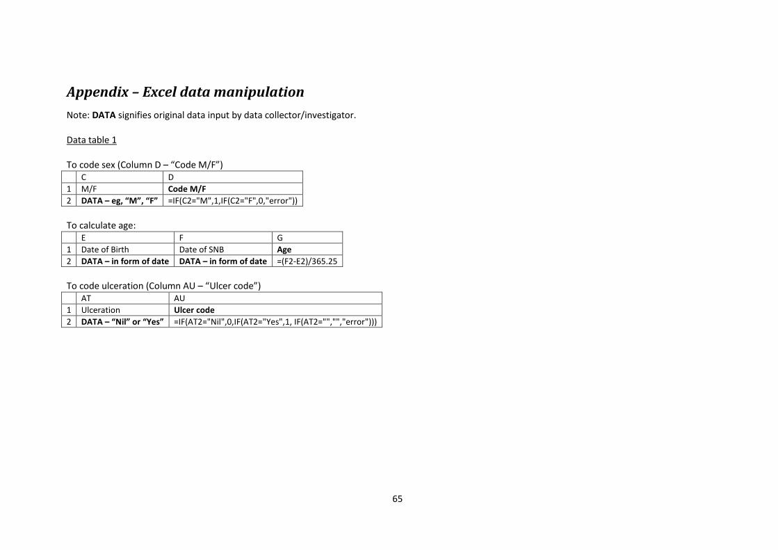
65

Appendix – Excel data manipulation Note: DATA signifies original data input by data collector/investigator.

Data table 1

To code sex (Column D – “Code M/F”) C D 1 M/F Code M/F 2 DATA – eg, “M”, “F” =IF(C2="M",1,IF(C2="F",0,"error")) To calculate age: E F G 1 Date of Birth Date of SNB Age 2 DATA – in form of date DATA – in form of date =(F2-E2)/365.25 To code ulceration (Column AU – “Ulcer code”) AT AU 1 Ulceration Ulcer code 2 DATA – “Nil” or “Yes” =IF(AT2="Nil",0,IF(AT2="Yes",1, IF(AT2="","","error")))

66

To code side (Column J – “Left or right”) and area of lymph node basin (Column T – “Final LN Area”) I J K L M N O P Q R S T 1 Area of

lymph node

Left or Right

Lnarea Groin Popliteal Axilla Epitrochlear

Triangular space

Neck Other Reclass Final LN area

2 DATA, eg, Rgroin, Laxilla

=IF(COUNTA(I2)=1,IF(ISERR(FIND("R",I2)=TRUE),IF(ISERR(FIND("L",I2))=TRUE,"error",IF(FIND("L",I2)=1,"0","2")),IF(FIND("R",I2)=1,"1","2")),"")

=IF(COUNTA(I2)=1,IF(ISERR(FIND("/",I2))=TRUE,IF(ISERR(FIND("axilla",I2))=TRUE,IF(ISERR(FIND("groin",I2))=TRUE,IF(ISERR(FIND("neck",I2))=TRUE,"error",3),2),1),4),"")

=IF($K2=4,IF(ISERR(FIND("groin",$I2))=FALSE,TRUE,FALSE),"")

=IF($K2=4,IF(ISERR(FIND("pop",$I2))=FALSE,TRUE,FALSE),"")

=IF($K2=4,IF(ISERR(FIND("axil",$I2))=FALSE,TRUE,FALSE),"")

=IF($K2=4,IF(ISERR(FIND("epit",$I2))=FALSE,TRUE,FALSE),"")

=IF($K2=4,IF(ISERR(FIND("triang",$I2))=FALSE,TRUE,FALSE),"")

=IF($K2=4,IF(ISERR(FIND("neck",$I2))=FALSE,TRUE,FALSE),"")

=IF($K2=4,IF(OR(L2,M2,N2,O2,P2,Q2)=TRUE,"",1),"")

=IF(K2=4,IF(AND(OR(L2,M2),NOT(OR(N2,O2,P2,Q2))),2,IF(AND(OR(N2,O2,P2),NOT(OR(M2,L2,Q2))),1,IF(AND(Q2,NOT(OR(P2,O2,N2,M2,L2))), 3,4))),"")

=IF(K2=4,S2,K2)

To extract number of positive lymph node (Column Y – “NoPos”) X Y 1 Histology NoPos 2 DATA, in the form of: “0\2”, “1\2” etc =IF(COUNTA(X2)=1,MID(X2,1,FIND("\",X2,1)-1),"") To extract tumour type code (Column AR – “Type code”) and thickness (Column AS – “Thickness”) from original data input (Column AP) AP AQ AR AS 1 Type, Thickness Type Type code Thickness 2 DATA, in the form of “SSM 1.3”, “NM

2.9”, etc =IF(COUNTA(AP2)=1,IF(COUNT(AP2)=1,"",MID(AP2,1,FIND(" ",AP2,1)-1)),"")

=IF(AQ2="","",IF(AQ2="SSM",1,IF(OR(AQ2="SSM/NM",AQ2="NM"),2,IF(AQ2="AL",3,IF(AQ2="LM",4,IF(AQ2="Des",5,IF(OR(AQ2="MIS",AQ2="Blue"),9,"error")))))))

=IF(COUNTA(AP2)=1,IF(COUNT(AP2)=1,AP2,MID(AP2,FIND(" ",AP2,1)+1,4)),"")

67

Table 2 – Events datasheet – working out a list of dates of distant recurrences

B C D E F G H I J K L M N O P Q R 1 PIN … … … … Date of

SNB This shaded area is a copy of a limited area

of the main datasheet (datasheet 1). This is simply to supply a list of SNB dates for lookup in the main data area below

2 741 2/1/2001 3128

… … … … … …

3132

PIN locoregional recurrence

PIN distant recurrence

PIN any recurrence

SNB date Event date Event type

Event description

Recurrence

Event description 2

Local/regional

distant

3133

=IF(AND(J3132=1,Q3132=1,G3132>F3132),B3132,"")

=IF(AND(J3132=1,R3132=1,G3132>F3132),B3132,"")

=IF(AND(J3132=1,G3132>F3132),B3132,"")

=VLOOKUP(B3132,$A$2:$G$3128,7,FALSE)

DATA – in form of date

DATA – in form of event colde

DATA – eg, “Treatment”, “Recurrence”

=IF(I3132="Recurrence",1,0)

=IF(I3132="Date of birth",1,0)

=IF(I3132="Primary Melanoma",1,0)

=IF(I3132="Treatment",1,0)

=IF(I3132="Last status",1,0)

=SUM(J3132:N3132)

DATA – eg, “Surgery: local” or “Dead melanoma”

=IF(J3132=1,IF(OR(NOT(ISERR(FIND("Regional",P3132)))=TRUE,NOT(ISERR(FIND("Local",P3132)))=TRUE,NOT(ISERR(FIND("locoregional",P3132)))=TRUE,NOT(ISERR(FIND("Extracapsular",P3132)))=TRUE,NOT(ISERR(FIND("transit",P3132)))=TRUE),1,""),"")

=IF(J3132=1,IF(ISERR(FIND("Distant",P3132))=FALSE,1,""),"")

68

..

. ... … … … …

29140

PIN 4 6 13 7 This shaded area of the data table is the output area. It was then copied to the main datasheet in Excel (Sheet 1), then to Stata. This represents a table with a list of PINs, date of distant recurrence, and a censoring variable with 1 representing the occurrence of distant metastasis. A similar table was produced on a separate worksheet for locoregional recurrence.

29141

741 =IF(ISNA(VLOOKUP($B29140,$D$3131:$Q$29122,C$29139,FALSE))=TRUE, "",VLOOKUP($B29140,$D$3131:$Q$29122,C$29139,FALSE))

=IF(ISNA(VLOOKUP($B29140,$D$3131:$Q$29122,D$29139,FALSE))=TRUE, "",VLOOKUP($B29140,$D$3131:$Q$29122,D$29139,FALSE))

=IF(ISNA(VLOOKUP($B29140,$D$3131:$Q$29122,E$29139,FALSE))=TRUE, "",VLOOKUP($B29140,$D$3131:$Q$29122,E$29139,FALSE))

=IF(ISNA(VLOOKUP($B29140,$D$3131:$Q$29122,F$29139,FALSE))=TRUE, "",VLOOKUP($B29140,$D$3131:$Q$29122,F$29139,FALSE))

… … … … …