world urbanization prospects the 2014 revision · 4 united nations department of economic and...

E c o n o m i c &

World Urbanization Prospects The 2014 Revision Methodology

United Nations New York, 2014

S o

c i a

l A f f a

i r s

ESA/P/WP/238

Department of Economic and Social Affairs Population Division

World Urbanization Prospects The 2014 Revision Methodology

United Nations New York, 2014

DESA

The Department of Economic and Social Affairs of the United Nations Secretariat is a vital interface between global policies in the economic, social and environmental

spheres and national action. The Department works in three main interlinked areas: (i) it compiles, generates and analyses a wide range of economic, social and environmental data and information on which States Members of the United Nations

draw to review common problems and take stock of policy options; (ii) it facilitates the negotiations of Member States in many intergovernmental bodies on joint courses of action to address ongoing or emerging global challenges; and (iii) it advises interested

Governments on the ways and means of translating policy frameworks developed in United Nations conferences and summits into programmes at the country level and, through technical assistance, helps build national capacities.

Note

The designations employed in this report and the material presented in it do not imply the expression of any opinion whatsoever on the part of the Secretariat of the United Nations concerning the legal status of any country, territory, city or area or of its authorities, or concerning the delimitation of its frontiers or boundaries.

Symbols of United Nations documents are composed of capital letters combined with figures.

Suggested citation:

United Nations, Department of Economic and Social Affairs, Population Division (2014). World Urbanization Prospects: The 2014 Revision, Methodology Working Paper No. ESA/P/WP.238

This publication has been issued without formal editing.

United Nations Department of Economic and Social Affairs/Population Division 3 World Urbanization Prospects: The 2014 Revision, Methodology

PROCEDURES TO ESTIMATE AND PROJECT THE POPULATION OF URBAN AREAS AND URBAN AGGLOMERATIONS

Within the World Urbanization Prospects, the estimation and projection of the urban population is based on observed changes in the proportion of the population living in urban areas. Consequently, the quality of the estimates and projections depends on the quality of the basic information enabling the calculation of the proportion urban. Such information normally consists of complete counts of both the total population in a country and the total population living in urban areas. Censuses or population registers are the most common sources of those counts. To be accurate, the proportion urban should be based on counts of the total and the urban population that achieve similar levels of coverage and that reflect correctly the division of territory into urban and rural areas. Because of the complexity and variety of situations in which the urbanization process occurs, it is not always straightforward to divide the inhabited territory into urban and rural areas. Indeed, the criteria used to identify urban areas vary from country to country and may not be consistent even between different data sources within a given country. Furthermore, as the process of urbanization proceeds, the number and extension of the areal units qualifying as urban generally expand. Therefore, keeping an urban versus rural division of territory constant over time would be misleading and would likely result in a major underestimation of the actual proportion of the population living in areas with urban characteristics. In preparing estimates and projections of the urban population, the United Nations relies on the data produced by national sources, which reflect the definitions and criteria established by national authorities. Given the variety of situations in the world, it is not currently possible (or indeed even desirable) to adopt uniform criteria to distinguish urban areas from rural areas (see, for instance, United Nations, 1967 and 1969). For example, stipulating that any areal unit with at least 5,000 inhabitants should be considered urban is not appropriate in populous countries such as China or India where rural settlements with none of the characteristics typical of urban areas often have large numbers of inhabitants. Overall, national statistical offices are in the best position to establish the most appropriate criteria to characterize urban areas in their respective countries. No attempts have been made to impose consistency in definitions across countries. However, several efforts are underway at different institutions to produce globally comparable estimates of the urban population with uniform criteria to define urban areas based on satellite imagery of land cover or night-time lights. Nonetheless, to date, these approaches have not generated the long historical time series of urbanization estimates required for this report. The urban and city projections presented in this report are based on the definitions used for statistical purposes by the countries and areas themselves – except for cases lacking clear definitions, or historical changes that prevent reconstruction of consistent time series (e.g., Netherlands, Gambia, Kenya). One hundred and twenty-five of the 233 countries or areas considered use administrative criteria to distinguish between urban and rural areas. Sixty-five of these countries use administrative designations as the sole criterion (table 1). In 121 cases, the criteria used to characterize urban areas include population size or population density, and in 49 cases such demographic characteristics are the sole criterion. However, the lower limit above which a settlement is considered urban varies considerably, ranging between 200 and 50,000 inhabitants. Economic characteristics were part of the criteria used to identify urban areas in 32 countries or areas, including all the successor states of the former Union of Soviet Socialist Republics. Criteria related to the functional nature of urban areas, such as the existence of paved streets, water-supply systems, sewerage systems or electric lighting, were part of the definition of urban in 54 cases, but only in ten cases were such criteria used alone. Lastly, in seven cases no definition of “urban” was available and in eight cases the entire population of a country or area was considered to be urban.

4 United Nations Department of Economic and Social Affairs/Population Division World Urbanization Prospects: The 2014 Revision, Methodology

TABLE 1. DISTRIBUTION OF COUNTRIES ACCORDING TO THE CRITERIA USED IN DEFINING URBAN AREAS, 2014 REVISION

Number and type of criteria Sole use

Used in conjunction with

other criteria

Percentage according to

sole use

Percentage according to use in conjunction with

other criteria

1 criterion Administrative 65 60 27.9 25.8 Economic — 32 13.7 Population size/density 49 87 21.0 37.3 Urban characteristics 10 44 4.3 18.9 2 criteria Administrative and population size/density 26 — 11.2 — Administrative and economic — — — — Administrative and urban characteristics 12 — 5.2 — Economic and population size/density 14 — 6.0 — Economic and urban characteristics — — — —

Population size/density and urban characteristics 15 — 6.4 —

3 criteria Administrative, economic and population size/density 5 — 2.1 —

Administrative, economic and urban characteristics — — — —

Administrative, urban characteristics and population size/density 4 — 1.7 —

Economic, urban characteristics and population size/density — — — —

4 criteria Administrative, economic, population size/density and urban characteristics 13 — 5.6 —

Entire population size 10 10 4.3 4.3

Unclear definition 3 3 0.9 0.9

No definition 7 7 3.0 3.0

Total number of countries or areas 233 — 100.0 —

Despite the variety of criteria used to distinguish urban from rural areas and the resulting heterogeneity, no independent adjustment of national statistics was undertaken in this revision unless it was clear that the definitions used by a given country had changed over time in ways that would have led to inconsistencies. When applied, such adjustments typically eliminated the erratic peaks and troughs in urban growth resulting from changes in definition. Despite efforts to avoid inconsistencies within countries, it was not always possible to adjust the available data in ways that ensured consistency. In some cases, inconsistencies remained precisely because the data needed to make the necessary adjustment were lacking. In cases where adjustment was possible, every effort was made to adjust earlier data so that they conformed to the most recent definition. In the case of cities, population statistics are often reported in terms of the territory delimited by administrative boundaries that do not necessarily coincide with the extent of the urbanized territory as delimited by other standards. Thus, the “city proper” as defined by administrative boundaries may not include suburban areas where an important proportion of the population working or studying in the city resides. Furthermore, in some cases, two or more adjacent cities may be separately administered, although they might form jointly a single urbanized region. Alternatively, administrative boundaries of some cities may cover large tracts of land primarily devoted to agriculture. Because of these problems it is advisable to base the measurement of a city’s population on territorial boundaries that may differ from those established by the accidents of administrative history. Since they are less affected by changes in administrative boundaries, two auxiliary concepts have also been used to improve the comparability of


measurements of city populations across countries and over time. The first is the concept of an urban agglomeration, which refers to the population contained within the contours of contiguous territory inhabited at urban levels of residential density. The second is the concept of the metropolitan region, which includes both the contiguous territory inhabited at urban levels of residential density and additional surrounding areas of lower settlement density that are under the direct influence of the city (for example, through established transport networks, road linkages or commuting patterns). In compiling information on city population size for this revision, the Population Division endeavoured to use data or estimates based on the concept of urban agglomeration. When those data were not consistently available, population data that refer to the city as defined by its administrative boundaries were used. However, where administrative boundaries remain fixed for long periods of time, reliance on them can often result in an underestimation of the actual growth of a city with respect to both its territory and its population. Only when administrative boundaries change with relative frequency can one assume that they reflect the actual territorial expansion of the urbanized area. For a number of cities, the data available refer to two concepts: the city proper, as defined by administrative boundaries, and its metropolitan area. In those instances, the data referring to the metropolitan area were usually preferred because they are thought to approximate better the territory associated with the urban agglomeration than the data based on administrative boundaries. However, the population of the metropolitan area is also likely to be larger than that of the urban agglomeration associated with it, so an upward bias may have been introduced in specific cases. For many cities, an effort was made to ensure that the time series of population estimates derived from national sources conformed to the same definition over time. Adjustments were made when necessary to achieve internal consistency. In some cases, the availability of data determined that the criterion on which the population of a city is based should be changed. That was the case, for example, when data on a city in terms of the urban agglomeration were available for only one or two points in time, while a longer and more consistent series of data on the population of the city proper was readily available.

TABLE 2. DISTRIBUTION OF COUNTRIES OR AREAS ACCORDING TO THE CRITERIA USED IN DEFINING CITY POPULATIONS, 2014 REVISION

Criterion Sole use

Used in conjunction with

other criteria

City proper .................................... 89 48 Urban agglomeration .................... 79 48 Metropolitan area .......................... 11 10

Capital is urban agglomeration; other cities are city proper, urban agglomerations or metropolitan areas ......................... 28 —

Capital is city proper; other cities are city proper, urban agglomerations or metropolitan areas .............................................. 11 —

Capital is metropolitan area; other cities are city proper, urban agglomerations or metropolitan areas ......................... 13 — Not defined ................................... 1 1 Total number of countries or areas 232 —

In the 2014 Revision, the city data for 79 of the 232 countries or areas considered were based on the concept of urban agglomeration (table 2, above). In a further 28 countries, data for the capital city were reported in terms of urban agglomeration, whereas data for other cities referred to city proper, urban


agglomeration or metropolitan area. For an additional 89 countries or areas the city data available reflected a definition of a city proper. In 48 countries or areas different definitions were used for different cities. Adjustment of city data was carried out when information for a particular city had changed over time. Where possible, the urban agglomeration concept was used. However, when recent data were based on the concept of city proper and there was insufficient information to adjust the data to reflect the population in the urban agglomeration, a time series based on the city proper definition was used.

A. THE ESTIMATION OF URBAN INDICATORS OVER THE ESTIMATION PERIOD In addition to variations in the definition of what constitutes an urban area, the data available for different countries may also vary in terms of their time reference. Because census dates are not the same for all countries, estimates of the proportion urban or of city populations derived from census data typically refer to different points in time and are not directly comparable among countries. Similarly, there is no consistency among countries with respect to the reference dates of official estimates of urban or city populations. Consequently, in order to complete the 2014 revision of World Urbanization Prospects, estimates for specific points in time had to be derived. Interpolation or extrapolation based on the data available was used to produce estimates of the proportion urban or of city populations that referred to 1 July of the relevant calendar year, starting in 1950. The most recent mid-year estimate referred to the year that preceded the reference date of the most recent data available. From that point on, the projection procedure was used to complete the time series until 2050 for the proportion urban and until 2030 for city populations. Among the 233 countries or areas considered in this Revision, the proportion urban was analysed for over 1,850 observations with 8 observations per country on average. As seen on figure I, the proportion urban is most often available in the years around the start of each decade, due to the availability of new census data.

Figure I. Annual distribution of percentage urban

For 188 countries (81 per cent), the most recent data available refer to 2005 and later (table 3). Only for three countries (Myanmar, Democratic Republic of Congo, and Seychelles) did the most recent data refer to the 1980s. Clearly, when recent information on the proportion urban is available for a given country or area, it is more likely that projections over the short-term approximate true trends.

020

4060

80N

umbe

r of

obs

erve

d da

ta p

oint

s

1950 1960 1970 1980 1990 2000 2010 2020year


TABLE 3. DISTRIBUTION OF COUNTRIES OR AREAS ACCORDING TO MOST RECENT INFORMATION AVAILABLE

Date of most recent information

Number of countries or

areas Percentage

Before 1990 ............... 3 1.3

1990-1994 .................. 2 0.9

1995-1999 .................. 7 3.0

2000-2004 .................. 33 14.2

2005-2009 .................. 59 25.3

2010 and later ............ 129 55.4

TOTAL 233 100 .0

The proportion of the population living in urban areas was estimated and projected by country or area for the period 1950-2050 in single-year intervals. Once values of the proportion urban at the national level were established for the 1950-2050 period, they were applied to the estimates and projections of the total national population of each country or area derived from World Population Prospects: The 2012 Revision (United Nations, 2013) so as to obtain the corresponding urban population for 1950 to 2050. At a later stage, country-level estimates and projections were aggregated to obtain figures corresponding to regions, major areas and the world as a whole. Calculation of the proportion urban during the estimation period involved interpolation between recorded figures, and extrapolation back to 1 July 1950 when the earliest recorded figures referred to a later date. Such interpolation or extrapolation to 1950 is based on the urban-rural ratio (URRt), defined as the ratio of the urban to the rural population, that is:

tt

t

UURR

R=

(1)

where Ut and Rt denote the size at time t of the urban and the rural populations, respectively. The urban-rural ratio at time t is directly related to the percentage urban (PUt) because:

( ) ( )1

t tt

t t t

U URRPU

R U URR= =

+ + (2)

Let nrurt denote the growth rate of the urban-rural ratio between times t and t+n:

1 t nn t

t

URRrur ln

n URR+

= × (3)


Then, substituting URRt for its equivalent according to (1), it follows that:

( ) ( )

t n tn t

t n t

t+n t+n t t

t n t n

t t

t n t n

t t

n t n t

1 U Urur = ln - ln

n R R

1= ln U - ln R - ln(U ) + ln(R )

n

1 U R= ln - ln

n U R

1 U 1 R= ln - ln

n U n R

= u - r

+

+

+ +

+ +

×

×

×

× ×

(4)

where nut denotes the growth rate of the urban population between times t and t+n, and nrt is the growth rate of the rural population over the same interval. That is, the growth rate of the urban-rural ratio is equivalent to the difference between the growth rates of the urban and the rural populations. Therefore, nrurt is known as the urban-rural growth difference and is the basis for the interpolation and extrapolation of the proportion urban. Assuming a constant growth rate, if T is any time point within the intercensal period (t, t+n), it follows that:

( )n trur (T-t)T tURR = URR e ×× (5)

The same equation (based on the same assumption) can be applied to obtain extrapolated values of URR when T is outside the intercensal period and (t, t+n) is the intercensal period closest to it. The use of equation (5) for interpolation and extrapolation purposes relies on an assumption that rur remains constant during each intercensal period, and during the period from 1950 to the reference date of the first observation available. Once an estimate of URRT is available, it can be converted to PUT with equation (2).

B. PROJECTION OF THE PROPORTION URBAN AT THE NATIONAL LEVEL The United Nations has developed a parsimonious and straightforward method to project the proportion urban. The method was first used in the 1970s (United Nations, 1974 and 1980) and, although it has undergone some revisions since then, the basic approach has not changed. The method projects the most recently observed urban-rural growth difference by assuming that the proportion urban follows a logistic path that attains a maximum growth rate when the proportion urban reaches 50 per cent and whose asymptotic value is 100 per cent. Normally, an extrapolation based on a simple logistic curve would imply that the urban-rural growth difference would remain constant over the projection period. Yet empirical evidence shows that the urban-rural growth difference declines as the proportion urban increases because the pool of potential rural-urban migrants decreases as a fraction of the urban population, while it increases as a fraction of the rural population. Consequently, a model for the evolution of the urban-rural growth difference was developed so that it would evolve over the projection period, passing from the last observed value to a world norm consistent with historical experience. The norm is expressed in terms of a hypothetical urban-rural growth difference, denoted by hrur. For the 2014 revision, the hypothetical urban-rural growth difference, was obtained by regressing the urban-rural growth difference during any given time interval on the percentage urban at the mid-point of the corresponding time interval, for the 148 countries or areas


with 2 million or more inhabitants in 2013. The resulting regression equation1 estimated on 1,068 observations (with 926 observations covering the period 1950-2013 and 142 observations for the period 1800-1949) is as follows:

�ℎ�� = 0.030588 − 0.020508 × ��(��

�

�) (6)

where ��(��

�

�) is the proportion urban for the mid-point of the intercensal period between times t and t+n.

Figure II shows all the observations considered (with green dots representing observations since 1950 and red dots representing observations before 1950) together with the fitted regression line in orange. The empirical experience of several countries through the last one or two centuries illustrates how the observed urban-rural growth difference, denoted by rur, has changed over time as populations became more urban (PU). Equation (6) implies that, as the initial level of urbanization increases, hrur decreases. When the initial proportion urban is zero, an urban-rural growth difference of 0.030588 can be expected; when the proportion urban is 0.5, a value of hrur of 0.020334 can be expected. When the proportion urban reaches 1, no further growth in the percentage urban can occur; therefore at that point hrur is set equal to zero.

For the 83 countries or areas with less than 2 million inhabitants in 2013 (many of them are islands or enclaves), another regression equation2 was estimated based on 521 observations (with 470 observations covering the period 1950-2013 and 51 observations for the period 1812-1949), and reads as follows:

�ℎ�� = 0.016892 − 0.006998 × ��(��

�) (7)

Figure II. Growth rate of the urban-rural ratio (rur) by proportion urban (PU) for countries or areas with 2 million or more inhabitants in 2013: selected country trajectories and fitted robust regression model

1 Robust regression estimated using Stata/SE 12.0 for Windows (64-bit). Five extreme outliers associated with exceptional historical events where |rur| > 0.2 were excluded from this analysis. R2= 0.03 2 Robust regression estimated using Stata/SE 11.2 for Windows (32-bit). Three extreme outliers associated with exceptional historical events where |rur| > 0.2 were excluded from this analysis. R2= 0.002

-.05

0.0

5.1

.15

RU

R (

grow

th r

ate

of th

e ur

ban-

rura

l rat

io)

0 .2 .4 .6 .8 1PU (proportion urban)

1950-2013 observations < 1950 observations

Robust reg (All years) 2+ m. 1953-2010 China

1901-2013 India 1921-2000 Ghana

1950-2010 Mexico 1806-2006 France

1800-2010 Sweden 1950-2000 USA


Figure III shows all the observations analysed and the fitted regression line (in orange). The trajectories since the 1950s (or earlier) for selected countries illustrate how rur has changed over time with greater urbanization (PU).

Figure III. Growth rate of the urban-rural ratio by proportion urban for countries or areas with less than

2 million inhabitants in 2013: selected country trajectories and fitted robust regression model

The projection of the proportion urban is based on the projection of the urban-rural growth differential. It is assumed that the most recently observed urban-rural growth difference in a given country converges to the hypothetical urban-rural growth difference, or world norm, over a period of 25 years. The projection is set to start at time t0, the time at the most recently observed PU, and is carried forward until the year 2050. The projection method has been modified slightly in two ways in this revision. First, because the world norm is a decreasing function of the percentage urban, the convergence of the projected urban-rural growth differential to the world norm was not assumed to be exactly linear. Rather, the projected urban-rural growth difference, denoted by rur*, was obtained recursively as follows:

��∗ = ��∗� + ��(�)��∗

� �(��)� for all t< t0+25 (8)

This ensures that the projected rur* approaches the world norm smoothly in consonance with the contemporary level of the percentage urban, and that at t= t0+25, the projected rur* attains the world norm evaluated at the corresponding level of urbanization. Second, for t > t0+25, rather than keeping rur* constant at the level of the world norm, rur* was set to track the hrur that corresponds to the projected level of PU. In other words,

��∗ = ℎ��(��) for t0+25 ≤ t ≤ ω (9)

where ω is the last year of the projection, 2050.

-.1

0.1

.2R

UR

(gr

owth

rat

e of

the

urba

n-ru

ral r

atio

)

0 .2 .4 .6 .8 1PU (proportion urban)

1950-2013 observations < 1950 observations Robust reg (All years) <2 m.

1881-2007 Cyprus 1921-2006 Maldives 1921-2010 Liechtenstein

1930-2010 Iceland 1946-2000 Trinidad and Tobago 1950-2001 Bahrain


Then, the urban-rural ratio was calculated as:

�� = �� × ��∗ (10)

Each projected value of URRt was then converted into a proportion urban PUt using equation (2).

In order to derive the urban population at the national level, the proportion urban was multiplied by the total population of each country, obtained from the independent estimates and projections published in World Population Prospects: The 2012 Revision (United Nations, 2013). With respect to the estimates and projections of the urban population at the regional level, the urban populations of all countries in the appropriate region were cumulated. Lastly, regional totals were aggregated to derive estimates and projections at the world level.

C. PAST ESTIMATES OF CITY POPULATIONS

Estimates and projections of the population of cities with an estimated population of 300,000 inhabitants or more in 2014 were calculated for the period 1950-2030. However, in order to carry out a more comprehensive monitoring of population growth in cities, all those reaching a population of 100,000 or more within the 1950-2014 period were also considered, provided data on their population size was available from a census or population register3. Cities of 300,000 inhabitants or more in 2014 are illustrated on Map I by size class of urban settlement.

Map I. Cities by size class of urban settlement, 2014

NOTE: The boundaries and names shown and the designations used on this map do not imply official endorsement or acceptance by the United Nations.

3 Furthermore, once a city has reached 100,000 inhabitants, its population size continues to be monitored by the Population Division even if the population subsequently falls below the 100,000 person level, provided national statistical sources continue to report data. For the 2014 Revision, 5,334 cities or urban agglomerations were considered (including 1,428 cities of less than 100,000 persons in 2014).


City population data were analysed for over 38,000 observations with on average 7 observations per city (and a standard deviation of 4 observations). As seen in figure IV, city population data are most often available in the years around the start of each decade, reflecting the importance of census data as the primary source of information on the size of city populations.

Figure IV. Annual distribution of city populations

For 4,546 cities or urban agglomerations (85 per cent), the most recent data available referred to 2005 and later (table 4). Because countries take population censuses at different times, the actual dates of observation vary from city to city, although they are usually identical for cities within a particular country. Just as with the estimates of the proportion urban, while preparing estimates of city populations it was necessary to estimate the population size of all cities for the same reference dates in the past.

TABLE 4. DISTRIBUTION OF CITIES OR URBAN AGGLOMERATIONS ACCORDING TO MOST RECENT INFORMATION AVAILABLE

Date of most recent information

Number of cities or urban agglomerations Percentage

Before 1990 .......................... 28 0.5

1990-1994 ............................. 27 0.5

1995-1999 ............................. 91 1.7

2000-2004 ............................. 642 12.0

2005-2009 ............................. 795 14.9

2010 and later.................. 3,751 70.3

TOTAL 5,334 100.0

050

010

0015

0020

00N

umbe

r of

obs

erve

d da

ta p

oint

s

1950 1960 1970 1980 1990 2000 2010 2020year


To estimate the population of cities on 1 July of any year in the past, the procedure used is similar to the one described above for the proportion urban. However, in this case, instead of using the urban-rural growth difference, the interpolation or extrapolation is based on the difference between the growth rate of a city and the growth rate of the population of the rest of the country. Specifically, one considers the ratio of the city population at time t, Ct , to the population of the rest of the country, RESt:

tt

t

CCRR

RES=

(11)

where

t t tRES P C= − (12)

and Pt is the total population of the country at time t. The growth rate of CRR between t and t+n, denoted by nrcrt , is

( ) ( )1

n t t n trcr ln CRR ln CRRn + = × −

(13)

which is equivalent to

n t n t n trcr c res= − (14)

where nct is the growth rate of the city’s population between t and t+n, and nrest is the growth rate of the rest of the country’s population between t and t+n. Assuming constant growth rates, the value of CRR for any time T within the period (t, t+n) is given by:

( )( )n trcr T t

T tCRR CRR e× −= × (15)

The same equation can be applied to obtain extrapolated values of CRR when T is outside the intercensal period (t, t+n) and that period is the closest to T. The ratio of a city’s population to the total population of a country at time T, PCT , is equivalent to:

1T

TT

CRRPC

CRR=

+ (16)

To obtain interpolated or extrapolated estimates of city size, the proportion PCt was calculated for time T and multiplied by an independent estimate of the country’s population to obtain the population of the city at time T. Such independent estimate was obtained from the country-level estimates published in World Population Prospects: The 2012 Revision (United Nations, 2013).

D. THE PROJECTION OF CITY POPULATIONS

The method used for projecting city populations is similar to that used for urban populations. The city growth rate over the most recent intercensal period is modified over the projection period so that it approaches linearly an expected value that is based on the city population and on the growth rate of the urban population as a whole. First, if (t, t+n) is the most recent intercensal period for a given country or, more specifically, the period between the two most recent sets of observed city populations, the city-urban growth difference, denoted by ��, is calculated as:

�� = �� − �� (17)

that is, the difference between the rate of population growth for the city and that for the total urban population. To project a city’s population it is necessary to establish future values of �� using a model.


The model used to project �� was developed by regressing the observed values of �� for the most recent period for which data were available for each city on the logarithm of the city’s population at the beginning of that period. The regression equation was fitted4 to the data relative to 5,305 cities located in the 232 countries or areas analysed (28,931 observations including 24,292 observations covering the period 1950-2013 and 4,639 observations for the period 1815-1949). Figure V shows all the observations considered (green dots indicate observations since 1950 and red dots indicate observations before 1950 for countries or areas with at least 2 million inhabitants in 2013; blue dots indicate observations from countries or areas with less than 2 million inhabitants in 2013) together with the fitted regression line in orange. The empirical experience of several cities through the last one or two centuries illustrates how rcu has changed over time with the growth of the population of these cities.

Figure V. Growth rate of the city-urban difference by city population (log) for all countries

or areas: selected city trajectories and fitted robust regression model

4 Robust regression estimated using Stata/SE 12.0 for Windows (64-bit). 62 extreme outliers associated to exceptional historical events with rcu > |0.25|, and 11 observations referring to city population less than 100 inhabitants were excluded from this analysis. R2= 0.0554

-.1

0.1

.2R

CU

(C

ity-U

rban

gro

wth

diff

eren

ce)

5 10 15 20log(city pop)

1950-2013 observations (2+ m.) < 1950 observations (2+ m.) Countries < 2 millions

rcu fitted robust regression 1843-1998 Karachi 1871-2006 Lagos

1840-2011 Budapest 1862-2012 Bruxelles-Brussel 1901-2011 Delhi

1950-2010 Ciudad de México (Mexico City) 1950-2010 Rio de Janeiro 1960-2010 Tokyo


Although the correlation between the city-urban growth difference and the logarithm of the initial population size of each city is low (R2

= 0.0554), taking account of the influence of population size on city growth dampened the growth of the largest cities in a manner that seems plausible. The fitted model is the following:

�� = 0.0547143 − 0.003383 × ��− 0.3086313 × �� − 0.001116 × �� × �� (18)

where ��is the population of the city at time t, �� is the growth rate of total urban population, and � ��× �� is the interaction term between these two variables. That is, at a given urban population growth rate, �� decreases as the population of the city increases. Equation (18) was used recursively to calculate �� over the projection period. Thus, if the projection period started at time T and the hypothetical growth rate of a city’s population over the period (T-n, T) was denoted byℎ�� , it was calculated as follows:

ℎ�� = �� + �� (19)

To deal with more specific constraints experienced by cities located in islands, enclaves and other small areas, regression equation (18) was also fitted5 on the subset of the data relative to 211 cities located in the 84 countries or areas that had less than 2 million inhabitants in 2013 (1,338 observations including 1,072 observations covering the period 1950-2013 and 266 observations for the period 1815-1949), which yielded the following model:

�� = 0.016546 + 0.000054 × �� − 0.501701 × �� − 0.04621 × �� × �� (20)

where �� is the population of the city at time t, �� is the growth rate of total urban population, and � ��× �� is the interaction term between these two variables. Regression (20) instead of (18) was used in equation (19) for cities located in countries or areas that had less than 2 million inhabitants in 2013. Figure VI shows all the observations considered (green dots represent observations since 1950 and red dots represent observations before 1950 for countries or areas with less than 2 million inhabitants in 2013) together with the fitted regression line in orange. In addition, the empirical experience of several cities through the last one or two centuries illustrate how rcu has changed over time with the growth of the population of these cities. A city’s growth was then projected according to equation (21). As in the approach for projecting the growth rates for the proportion urban (see equation 7), equation (21) includes weights to let the estimated growth rate converge to the hypothetical growth rate:

( ) ( )( )n T t n T-n t n T-nc = W c + 1-W hc× × (21)

The weights Wt were calculated as:

0 0

0

11 ( ) ( )

0 ( )t

t t t t dW d

t t d

− × − − ≤= − > (22)

5 Robust regression estimated using Stata/SE 12.0 for Windows (64-bit). 12 extreme outliers associated to exceptional historical events with rcu > |0.25|, and 2 observations referring to city population less than 100 inhabitants were excluded from this analysis. R2= 0.4096


Figure VI. Growth rate of the city-urban difference by city population (log) for countries or areas with less than 2 million inhabitants in 2013: selected city trajectories and fitted robust regression model

Projection calculations were carried out independently for each city within a country, but a further adjustment sometimes had to be made once the projected populations of all cities were available. If the aggregated projected values of the city populations of a country grew more rapidly than the total urban population of the country, a further dampening factor was imposed on the city growth rates. When this situation arose, the growth rate of each city was reduced by the following quantity:

( )n t n t t

n tt

rtc - u TC =

Uδ

× (23)

where TCt is the aggregated population of cities whose populations are being projected at time t, Ut is the total urban population, nrtct is the growth rate of the aggregated population of cities and nut is the growth rate of the urban population. That is, the projected growth rate of the city was changed to:

*

n t n t n tc c δ= − (24)

This reduction assures that the total population of cities will not exceed the total urban population, while maintaining the differences in the growth rates among cities.

-.1

0.1

.2R

CU

(C

ity-U

rban

gro

wth

diff

eren

ce)

4 6 8 10 12 14log(city pop)

1950-2013 observations (< 2 m.) < 1950 observations (< 2 m.) rcu fitted robust regression (< 2 m.)

1801-2010 Reykjavík, Iceland 1812-2011 Vaduz, Liechtenstein 1792-2008 Monaco

1753-2010 Gibraltar 1910-2011 Podgorica, Montenegro 1921-2006 Saint-Denis, Reunion

1901-2011 Port Louis, Mauritius 1881-2011 Lefkosia (Nocosia), Cyprus 1839-2011 Luxembourg, Luxembourg


Adjustments were also made to the projected growth rates of cities when the future city-urban growth difference (rcu) from equation (18) was less than zero; in such cases, rcu was set to zero. Similarly, if the hypothetical growth rate for a city (equation 19) was less than or equal to zero, the hypothetical growth rate was also set to zero. However, this second constraint was not enforced when the urban population was declining and the city population was growing (e.g., some Eastern European countries). In all cases, equation (21) was used to project the city growth rate. However, in instances when both the urban population and the city population were declining, only the projected city growth was used (i.e.,

*n tc with Wt=1 for all t). In addition, the projection using equation (21) started from 2014 onward, except when the urban population and the city population were both growing; in those instances, the projection started from the last observed time point. Finally, it should be noted that in many countries we have not been able to compile population figures for all urban settlements that are part of the urban environment. Therefore, in order to ensure greater consistency with the projected ratio between the sum of the urban settlements for which time-series of population estimates were available and the overall urban population, an additional step was undertaken in this revision. In that regard, the population of all other urban settlements for which estimates in a given country were unavailable was projected as a “single urban unit” as of 2014. This was done by applying the future annual growth rate of the urban population of each country to the estimated residual population, that is the difference between the total urban population and the sum of the cities for which city-level information was available.

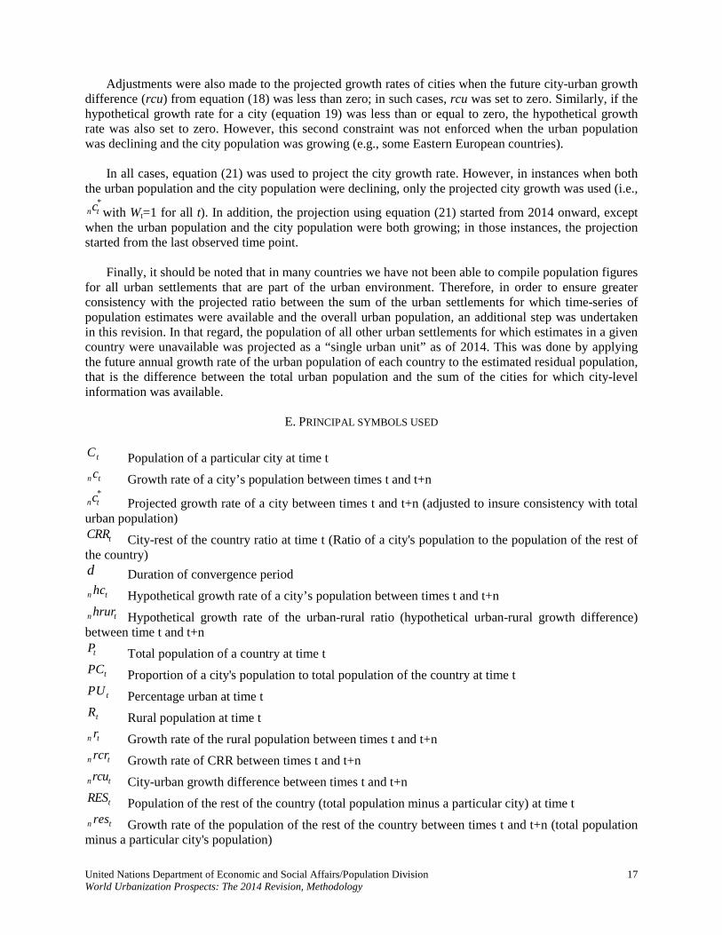
E. PRINCIPAL SYMBOLS USED

tC Population of a particular city at time t

n tc Growth rate of a city’s population between times t and t+n *

n tc Projected growth rate of a city between times t and t+n (adjusted to insure consistency with total urban population)

tCRR City-rest of the country ratio at time t (Ratio of a city's population to the population of the rest of the country) d Duration of convergence period

n thc Hypothetical growth rate of a city’s population between times t and t+n

n thrur Hypothetical growth rate of the urban-rural ratio (hypothetical urban-rural growth difference) between time t and t+n

tP Total population of a country at time t

tPC Proportion of a city's population to total population of the country at time t

tPU Percentage urban at time t

tR Rural population at time t

n tr Growth rate of the rural population between times t and t+n

n trcr Growth rate of CRR between times t and t+n

n trcu City-urban growth difference between times t and t+n

tRES Population of the rest of the country (total population minus a particular city) at time t

n tres Growth rate of the population of the rest of the country between times t and t+n (total population minus a particular city's population)


n trtc Growth rate of the aggregated population of cities between times t and t+n

n trur Growth rate of the urban-rural ratio (the urban-rural growth difference) between times t and t+n *

n trur Projected growth rate of the urban-rural ratio (urban-rural growth difference) between times t and t+n

tTC Aggregated population of cities at time t,

tU Urban population at time t

n tu Growth rate of the urban population between times t and t+n

tURR Urban-rural ratio at time t (ratio of the urban to the rural population)

tW Weight at time t

tnδ Dampening factor for city growth rates between times t and t+n t Index for time point n Length of time period

General:

A subscript on the lower left means the length of an interval, here in years.

A subscript on the lower right stands for time.

Superscripts are used to assign additional attributes to a symbol.

world urbanization prospects the 2014 revision · 4 united nations department of economic and...

Documents