1

World Oil Production Trend: How U.S. Shale Oil Production Changes the Trend

By Douglas B. Reynolds

Professor Oil and Energy Economics

Candace Crews 303 Tanana Dr. Rm 201

University of Alaska Fairbanks School of Management

Fairbanks, Alaska 99775-6080 (907) 474-6531, fx (907) 474-5219

The US has large reserves of shale gas and shale oil which look to make the US a net energy exporter within ten years. In addition, worldwide shale resources in China, Russia, Poland and France could mean that potential world oil production could double or triple in the next few decades. However, not all of these new reserves may be as large or as productive as North Dakota’s Bakken shale oil, therefore an alternative method of forecasting world oil supplies needs to be considered. In this article, we will look at a modified Hubbert curve forecast, although with some defined parameters. First, natural gas and oil need to be looked at as separate energy resources that are under separate markets and that are not perfect substitutes for each other. Next, it must be understood that the reserves of shale oil look to be a lot less in relative terms than the reserves of shale gas as evidenced by the price of natural gas in the US compared to the price of oil. This suggests that US and world supplies of shale oil will be limited. Finally, we look at possible world oil production trends rather than just US oil production trends. Two interesting comparisons of the world oil production trend to other regional trends are the former Soviet Union’s oil production trend and the U.S. oil production trend. If we compare the current world oil production trend to those previous trends using indexation, then we can get an idea of what may happen to world oil production in the future.

Key Words: World Oil Production, Shale Oil, Production Trends

2

World Oil Production Trend: How U.S. Shale Oil Production Changes the Trend

1. Introduction

We are in an oil crisis. It doesn’t appear as such since oil production from tar-sands and shale oil has been rising quickly causing the price of oil to stabilize around $100 per barrel. However, had not those alternative oil supplies been developed in a timely manner, we would have had an oil price shock that could have caused hyper-inflation and economic decline. Even at $100 per barrel, oil prices still are having a detrimental effect on the world’s tenuous post recession performance. So far, world oil supplies have kept rising due to shale oil and tar sands production, but that will not last forever. Therefore it is important to understand what the future supplies of oil will be.

When we consider energy in general, there are numerous supply sources and substitution strategies. However, if these other sources and substitution strategies are so numerous and powerful, then the price of oil should not have gotten so high. The fact that oil prices are high and have been high now since the first plateau of oil in 2005 suggests that there is a problem with substituting for oil. In fact if we look more closely at energy in general and oil in particular, there are three basic economic needs that energy is used for: 1) Electric power and electric power technologies; 2) Space heating for consumers and process heating for industry, and 3) personal private transportation, cargo transport and movement. As long as there is plenty of coal and natural gas, the heating and electric power issues are not a problem. It is only in the transportation, cargo transport and movement sectors where a dense, light, liquid fuel is necessary, mostly for large independent mobile machinery (LIMMs) such as automobiles, trucks and large movable equipment. Such LIMMs induce much economic growth and consumer value. Therefore it should be clear that we do not have an overriding energy problem or crisis, but rather we have a specific problem with oil and that there are not a lot of good substitutes for oil.

As far as LIMMs are concerned, it is very difficult to substitute electricity, natural gas and coal for dense liquid fuels. So far such substitutions as coal-to-liquids, gas-to-liquids and electric batteries for automobiles have been shown to be fairly expansive, and therefore we consider only conventional oil, tar-sands and shale oil supply. This means the world’s considerable economic output is very dependent on relatively cheap, liquid fuels for its survival and so we need to emphasize the supply and demand of liquid fuels, and especially oil, as a worldwide strategic necessity.

In order to understand the supply of oil, Reynolds (1999) and Hubbert (1956 and 1962) suggest the need to understand the mineral economy model and the Hubbert curve. The Hubbert curve and the mineral economy model are important methods for understanding non-renewable supply. To not include the Hubbert curve in resource studies, is to not actually understand non-renewable natural resource economics. Therefore in this article, we give a brief history of the Hubbert curve. Furthermore, since statistical analysis, such as Simmons (2005), shows that the world production of conventional oil has reached a peak, then the supply of energy for LIMMs is limited. What we don’t know is what will happen to shale-oil and tar-sands production going forward and how much of a supply boost they can give. One way to try to forecast the supply of conventional and non-conventional oil is to analyze previous Hubbert curve cycles, which can be used to forecast potential supplies.

In this paper, we consider a Hubbert curve forecast to try to determine how long and how much the current worldwide rise in oil production will last. We will do this by comparing the current world oil production pattern to that of other regions. This will help in understanding how long oil prices may remain stable as the world’s economy proceeds forward. While the current Hubbert cycle looks to peak in 2050, alternative forecasts could see world oil production peaks as early as this year. 2. A Potential Play

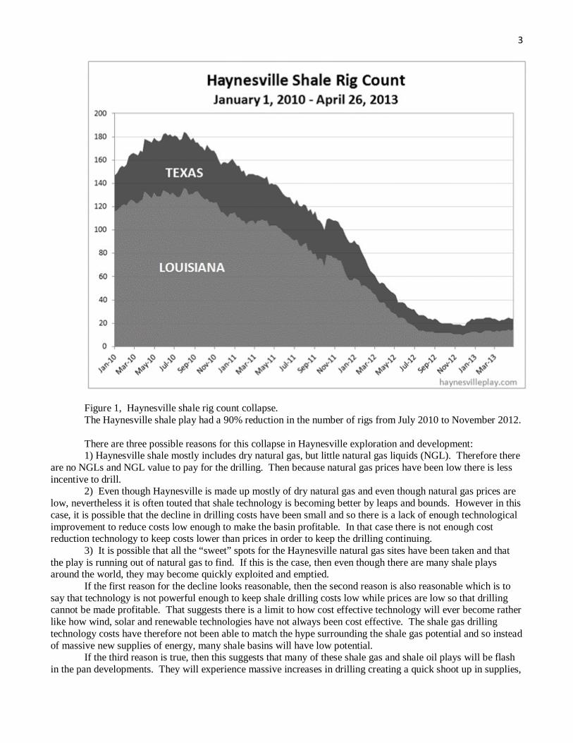
Consider a specific shale play and its drilling trend in Figure 1. That figure shows the Haynesville shale basin rig count over the last few years and shows the drilling declining by roughly 90%. Why would there be such a huge decline in drilling since it is often stated that shale plays have potentially huge supplies of energy?

3

Figure 1, Haynesville shale rig count collapse. The Haynesville shale play had a 90% reduction in the number of rigs from July 2010 to November 2012. There are three possible reasons for this collapse in Haynesville exploration and development: 1) Haynesville shale mostly includes dry natural gas, but little natural gas liquids (NGL). Therefore there

are no NGLs and NGL value to pay for the drilling. Then because natural gas prices have been low there is less incentive to drill.

2) Even though Haynesville is made up mostly of dry natural gas and even though natural gas prices are low, nevertheless it is often touted that shale technology is becoming better by leaps and bounds. However in this case, it is possible that the decline in drilling costs have been small and so there is a lack of enough technological improvement to reduce costs low enough to make the basin profitable. In that case there is not enough cost reduction technology to keep costs lower than prices in order to keep the drilling continuing.

3) It is possible that all the “sweet” spots for the Haynesville natural gas sites have been taken and that the play is running out of natural gas to find. If this is the case, then even though there are many shale plays around the world, they may become quickly exploited and emptied.

If the first reason for the decline looks reasonable, then the second reason is also reasonable which is to say that technology is not powerful enough to keep shale drilling costs low while prices are low so that drilling cannot be made profitable. That suggests there is a limit to how cost effective technology will ever become rather like how wind, solar and renewable technologies have not always been cost effective. The shale gas drilling technology costs have therefore not been able to match the hype surrounding the shale gas potential and so instead of massive new supplies of energy, many shale basins will have low potential.

If the third reason is true, then this suggests that many of these shale gas and shale oil plays will be flash in the pan developments. They will experience massive increases in drilling creating a quick shoot up in supplies,

4 but then be followed by a quick peak and collapse. In that case, the Hubbert curve is exactly the analysis we need to use in regard to these supplies. Nevertheless, no matter the reason, this dramatic decline in drilling suggests that it is possible for shale plays to expand as well as contract and to do so rapidly, in which case the massive supplies of shale energy around the world could be a lot less than we are lead to believe. Either way it is important to understand the Hubbert curve in order to analyze shale oil supplies. 3. The Hubbert curve

The normal way to understand a Hubbert curve is to use a simple logistics function to describe the trend: QP=URR*a*exp(-a(t-to))/[1+exp(a(t-to))]2 (1) Where QP = the current rate of production; URR = ultimately recoverable reserves; t = time; to = the year

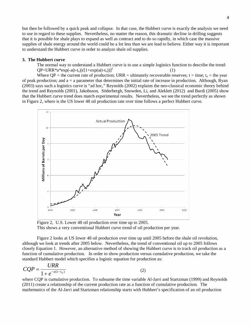
of peak production; and a = a parameter that determines the initial rate of increase in production. Although, Ryan (2003) says such a logistics curve is “ad hoc,” Reynolds (2002) explains the neo-classical economic theory behind the trend and Reynolds (2001), Jakobsson, Söderbergh, Snowden, Li, and Aleklett (2012) and Bardi (2005) show that the Hubbert curve trend does match experimental results. Nevertheless, we see the trend perfectly as shown in Figure 2, where is the US lower 48 oil production rate over time follows a perfect Hubbert curve.

Figure 2, U.S. Lower 48 oil production over time up to 2005. This shows a very conventional Hubbert curve trend of oil production per year. Figure 2 looks at US lower 48 oil production over time up until 2005 before the shale oil revolution,

although we look at trends after 2005 below. Nevertheless, the trend of conventional oil up to 2005 follows closely Equation 1. However, an alternative method of showing the Hubbert curve is to track oil production as a function of cumulative production. In order to show production versus cumulative production, we take the standard Hubbert model which specifies a logistic equation for production as:

)( 01 ttaeURRCQP −−+

= (2)

where CQP is cumulative production. To subsume the time variable Al-Jarri and Startzman (1999) and Reynolds (2011) create a relationship of the current production rate as a function of cumulative production. The mathematics of the Al-Jarri and Startzman relationship starts with Hubbert’s specification of an oil production

5 logistic model, which is the derivative of cumulative production with respect to time, QP = dCQP/dt which gives us equation 1. Rewriting equation 1, we get:

2)(

)(

]1[**

0

0

tta

tta

eeURRaQP −−

−−

+=

Next solve for )( 0tta −− in CQP and plug in to QP

2

2

2

2

22)(

)(

0

)(

****

11

1**

]1[**

1ln)(

1

0

0

0

CQPURR

aCQPa

CQPURR

URRaCQPURRa

QP

CQPURR

CQPURRURRa

eeURRaQP

CQPURRtta

CQPURRe

tta

tta

tta

−=−

=

−+

−

=+

=

−=−−

−=

−−

−−

−−

Re-label a as b1 and URR

a− as b2.

This becomes what Reynolds and Kolodziej (2009) call the “quadratic Hubbert curve.” 2

21 ** CQPbCQPbQP += (3)

b1 and b2 can be estimated econometrically to obtain URR by solving 2

1

bbURR −= . We can show the quadratic

Hubbert curve by re-specifying Figure 2 in terms of production versus cumulative production as Figure 3 shows.

6

Figure 3, U.S. Lower 48 oil production versus cumulative production up to 2005. This shows the same conventional Hubbert curve of Figure 2 only as a function of cumulative production rather than over time. This is called a quadratic Hubbert curve, since it exhibits a quadratic functional form of an inverted U. The same derivation also works for discovery

2** CQDURR

aCQDaQD −=

Where QD = the current rate of gas discovery; CQD = cumulative gas discovery to date for all previous periods for the entire region. Note that URR is a function of technology and regional characteristics, although Hubbert assumed small changes in technology over time were automatically included in the overall trend (Hubbert 1962 p.33). Hubbert (1956) very accurately predicted the US 1970 peak in oil production, although Brandt (2010) shows that many other geologists and petroleum experts also predicted it. Note also that Hubbert defines discovery as simply the difference in proven reserves from one year to another plus production, which simplifies the analysis so that reserves data do not have to be delineated between whether the reserve was found through wildcat drilling or through developmental drilling. Equation 3 is called a quadratic Hubbert curve or trend, which drives the mineral supply model. 1

Other energy exploration and production systems also follow a similar cumulative production trend such as nineteenth century whaling as shown in Figure 4 (see Bardi 2007).

1 Note, this equation and Hubbert’s original logistics curve are not arbitrary models; rather they are the result of Uhler’s (1976) information and depletion effects. This version of the Hubbert curve assumes that information and physical depletion is a function of cumulative discovery (or production) rather than a function of time.

7

Figure 4, Nineteenth century whaling. This shows the production of whale oil versus cumulative production. From Bardi (2007). One thing to remember about the Hubbert curve is that it must be defined over a specific mineral such as

conventional crude oil, whale oil, or shale oil. It is inappropriate to say we are not at peak oil because we can still produce, say, coal-to-liquids. The Hubbert curve is based on a specific mineral in a specific region, although here we do include shale oil with conventional oil as they use very similar technologies. In reality shale oil is a solid energy resource that must be converted into a liquid in-situ. Also the larger the region for which a production trend is tracked, the more rounded and close to the Hubbert logistics equation it will become.

4. Anomalies To The Hubbert curve

A number of countries do not seem to follow a normal Hubbert curve trend as Brandt (2007) shows. Reynolds (2011 and 2009) shows some specific countries where this lack of a Hubbert trend is found. When these countries’ oil production trends are indexed and compared to an indexed US trend up to 2005, i.e. the US trend that looked to exist before 2005 and which is extended to the 2005 expected ultimate recoverable reserves (URR), then this shows low rates of production for these other countries relative to their potential URR. These comparisons are shown in figures 5, 6, 7 and 8

Reynolds (2011b) and Reynolds et al. (2009) and Charness and Jackson (2009) suggest that one reason for the difference between the US and other oil producing countries is that the US has a competitive supply market where as many other oil producers include government owned oil companies, called monopoly national oil companies (NOC), which are risk averse. Whenever a government controlled business is created, there is a tendency for less risk taking, as such there is a tendency for a lower level of exploration and development of potential reserves in comparison to private, competitive institutions. After all Loderer (1985), Smith (2005a), Reynolds and Pippenger (2010), Kaufman et. al (2004) and Reynolds (2011b) show that OPEC as an organization is not effective in reducing its oil output by much, nevertheless, OPEC members do exhibit oil production

8 reductions. The reason for those reductions is likely to have been risk aversion, or possibly as in the case of Saudi Arabia due to an oil monopoly leader role, rather than due to cartel arrangements. Oil reductions are due to risk aversion, not market power.

Figure 5, US and Iranian Indexed Quadratic Hubbert Curve Oil Production Trend. This shows the indexed quadratic Hubbert curve of the US up until 2005 in comparison to Iran where 1 is the respective countries expected URR of conventional oil production, where the US uses its 2005 curve, from Reynolds (2009).

Figure 6, Kuwait and US Indexed Quadratic Hubbert Curve Oil Production Trend. This shows the indexed quadratic Hubbert curve of the US up until 2005 in comparison to Kuwait where 1 is the respective countries expected URR of conventional oil production, where the US uses its 2005 curve, from Reynolds (2009).

9

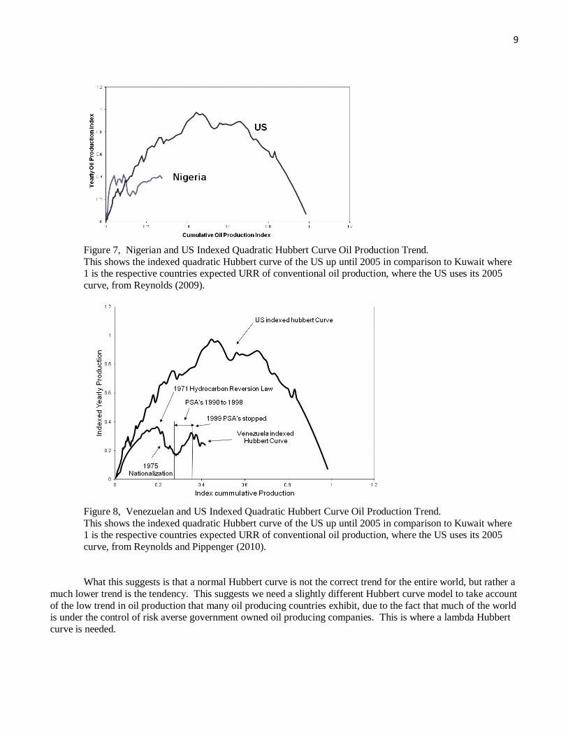
Figure 7, Nigerian and US Indexed Quadratic Hubbert Curve Oil Production Trend. This shows the indexed quadratic Hubbert curve of the US up until 2005 in comparison to Kuwait where 1 is the respective countries expected URR of conventional oil production, where the US uses its 2005 curve, from Reynolds (2009).

Figure 8, Venezuelan and US Indexed Quadratic Hubbert Curve Oil Production Trend. This shows the indexed quadratic Hubbert curve of the US up until 2005 in comparison to Kuwait where 1 is the respective countries expected URR of conventional oil production, where the US uses its 2005 curve, from Reynolds and Pippenger (2010). What this suggests is that a normal Hubbert curve is not the correct trend for the entire world, but rather a

much lower trend is the tendency. This suggests we need a slightly different Hubbert curve model to take account of the low trend in oil production that many oil producing countries exhibit, due to the fact that much of the world is under the control of risk averse government owned oil producing companies. This is where a lambda Hubbert curve is needed.

10 5. The World Lambda Hubbert curve

The world’s oil production does follow a Hubbert curve; however it is not the traditional quadratic Hubbert curve that we see in Equation 2 or shown in Figures 3 and 4. Instead, we would expect an abnormal Hubbert curve for the world, with a reduced production output. One way to model a reduced production output trend is with a lambda multi variable curve as shown in equation 4. QP = β1 • CQP - β2 • CQP1+λ (4)

If we use this curve and take an envelope of the world trend at the maximum oil production points of 1859, the starting point, 1973, the first major maximum inflection point, 1979 plus 4 mbd, the second major maximum inflection point minus the loss in Iranian oil production due to the revolution going on there at that time, and 2005, the third major maximum inflection point, we get a close approximation to the world trend. Figure 9 shows world production and the lambda trend up to 2009. Reynolds and Beak (2012) show that indeed the best explanation of the oil price rises and falls over the last 150 years is the relationship between consumption (demand) and the lambda Hubbert curve of equation 4 which represents the true Hubbert supply trend. Above the trend, the supply looks to be inelastic in the short run.

Figure 9, The World Lambda Hubbert Oil Production Trend. This shows the world lambda Hubbert trend up until 2009.

6. The World Multi-Cycle Hubbert Curve In figure 9, we see the lambda Hubbert curve up until 2009. Notice in Figure 10, however, when we go

beyond 2009, there is clearly a 2nd Hubbert cycle, a so-called multi-Hubbert cycle. Such a multi-Hubbert cycles as Reynolds and Kolodziej (2008, 2009), and Reynolds and Zhao (2007) show can be caused by changes in institutions, changes in prices or changes in technology. Indeed, if oil or natural gas prices rise above a threshold point, it is possible for there to suddenly be available new resources. Hubbert also shows just such a multi-cycle possibility in Hubbert (1963 p 32);

11

Figure 10, The World Lambda Multi-Cycle Oil Production Trend. After 2009, a second Hubbert cycle starts due to shale oil resources. What we would like to do is to discern what the 2nd cycle will look like going forward. Most

commentators simply look at the large size of the different shale basins around the world, such as the U.S. Bakken, Marcellus, Utica, and Haynesville plays and the Baltic Sea basin in Poland, the Bazhenov basin in Russia, the Paris basin in France and the Sichuan basin in China, and proclaim that these will provide shale oil at astronomical levels. They also suggest that shale oil supplies will be available at ever decreasing costs due to better technology and that therefore, this second cycle is unknowable and will increase two or three times above the first worldwide lambda oil production trend. However, if we look back at past Hubbert cycles for other large oil regions, we can discern different types of multi-cycle Hubbert potentials. Interestingly, the amount of oil coming out of the Bakken shale oil basin is about 700,000 barrels per day, where as the amount of oil coming out of the Haynesville shale oil basin is less than 10,000, because the Haynesville is a relative dry natural gas shale play and the Bakken is a relatively liquids rich shale oil play. Other shale basins also have different liquids or dry natural gas potential in denser or less dense formations at different locations in the basins, suggesting that sweet spots occur throughout any given basin. This suggests that many shale plays will see rising, then peaking, and then falling production cycles that will add up to a worldwide Hubbert production cycle.

12

Figure 11, The World Lambda Multi-Cycle Oil Production Trend and Price. This shows the world oil production trend with a multi-cycle. The second cycle is not causing the world oil price to go down. This suggests that a high price is needed to sustain this second multi-cycle trend. One of the interesting aspects about Figure 10 is what is happening to price. Notice in Figure 11, the real

price of oil over time is shown with the Hubbert trend and second Hubbert cycle. Whenever the demand (actual production) gets close to supply (the lambda Hubbert curve trend), the price of oil rises. However, after 2009, with a new Hubbert trend starting, the price of oil has not gone down, suggesting that oil needs about a $100 per barrel price in order to maintain this second Hubbert trend. In other words, as Reynolds and Kolodziej (2009) suggest, there may need to be a threshold price in order to sustain the second Hubbert cycle. However, we may assume that due to world growth, this $100 per barrel price will continue and that the shale oil and tar sands resources of the world will continue to increase in production following the new, second Hubbert cycle at least until this second cycle peaks.

However, the question is what will this new cycle look like. It may not be as large as expected and so future world oil supplies can still be tight. Also if the world growth rate continues, we might also expect that the new cycle will allow oil supplies to increase too slowly and still cause tight markets with rising prices. One idea to determine the future world oil supply, is to simply extend the current cycle along the track that it is currently following. This is shown in figure 12 where the current trend, and an expected future second cycle trend that started in 2009, are shown. The second 2009 trend is determined based on the very few years of increased production so far since 2009. Another idea, though, is to look at other multi-cycle Hubbert curves in history particularly for large regions and compare them to the current world trend.

13

Figure 12, The Extended World Lambda Multi-Cycle Oil Production Trend. If the current trend holds true, we can project world oil production’s next peak in about 2050.

7. Indexed Hubbert Curve Patterns

One way to model multi-cycle Hubbert trends is to add an indicator variable at a specific cumulative discovery amount, which can account for the effect of a specific institutional change or a specific price rise above a threshold price at a single point in time. The discovery model can be set up as follows:

QD = β0 + β1 • CQD + β2 • CQD1+λ + β3 • IND1 + β4 • IND1 • CQD + ε (5) where β’s are parameters and IND is a single dummy or indicator variable at a different time. The reason the single indicator variable is used in two terms is because in order for a second cycle to occur, both the intercept and the slope must change at the same point in time. However, since there may be more than one institutional change, more than one indicator variable can be added. For example QD = β0 + β1 • CQD + β2 • CQD1+λ + β3 • IND1 + β4 • IND1 • CQD + β5 • IND2 + β6 • IND2 • CQD + ε (6)

has two indicator variables for two different institutional changes at two different times. Even more indicator variables can be added as well until a model shows good statistical robustness. However, the justification for determining where the indicator variables are located and how many should be used has to come from specified institutional or price threshold changes. Consider some examples.

The US Multi-Hubbert Oil Production Cycle Example US oil production including both the Lower 48 and Alaska looks to have three different multi-cycle

Hubbert curves. See Figure 13. The first cycle, mostly due to the Lower 48 conventional oil, reached a peak and decline in 1970, then there looks to be a second small cycle, mostly due to Alaska, that started in 1977 and peaked in 1981. This second cycle was due to Alaska’s North Slope resources as explained in Reynolds and Zhao (2007). A third cycle has stared lately in 2008, where oil prices rose high enough to reach a threshold above which allowed much shale oil to be produced. The question is, when the second Hubbert cycle started, how far did people believe that these 2nd cycles would rise at the point in time of their inceptions. At the time of the US 2nd cycle in the mid 1970s, many speculated that the new US cycle would go well above the first US peak within ten years. Indeed, the government publication, Project Independence Report (1974) by the Federal Energy

14 Administration speculated that because of Alaska, because of offshore lower 48 oil and because of enhanced oil recovery (EOR) that US oil production was poised to take off to new heights of production within 10 years of the publication and consequently to go above the 1970 peak. However, once the second cycle got going, it quickly reached a second peak within 15 years of the first peak, 1985, but at a lower level than the first peak suggesting that an initial increase in the 2nd cycles should not have been seen necessarily as a vast new era of energy abundance. This same idea should color our thinking about the US 3rd cycle and about the world’s second Hubbert cycle.

Figure 13, The US 2nd and 3rd Oil Production Cycles. This shows how the U.S. had a 2nd and a 3rd cycle of oil production due to different institutional and price factors. The Former Soviet Union Multi-Hubbert Oil Production Cycle Example Another interesting example of a multi-cycle Hubbert curve is the former Soviet Union. The former

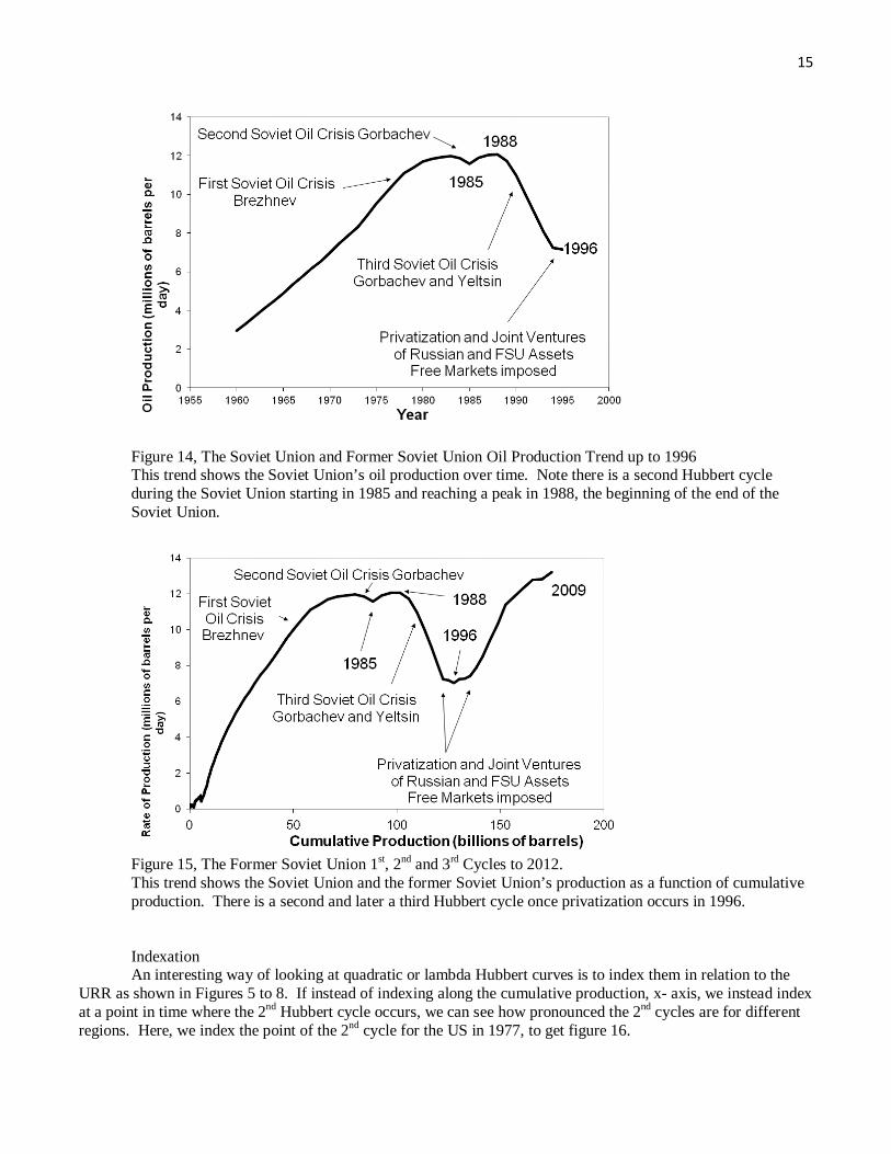
Soviet Union also shows an example of a 2nd and 3rd Hubbert cycle like the US. Notice in figure 14, the Soviet Union has an initial peak in oil production in 1983, and then after water flooding commences in 1985, a second peak occurs in 1988, followed by a complete collapse. A third cycle starts once Soviet oil fields are privatized in 1996.

15

Figure 14, The Soviet Union and Former Soviet Union Oil Production Trend up to 1996 This trend shows the Soviet Union’s oil production over time. Note there is a second Hubbert cycle during the Soviet Union starting in 1985 and reaching a peak in 1988, the beginning of the end of the Soviet Union.

Figure 15, The Former Soviet Union 1st, 2nd and 3rd Cycles to 2012. This trend shows the Soviet Union and the former Soviet Union’s production as a function of cumulative production. There is a second and later a third Hubbert cycle once privatization occurs in 1996. Indexation An interesting way of looking at quadratic or lambda Hubbert curves is to index them in relation to the

URR as shown in Figures 5 to 8. If instead of indexing along the cumulative production, x- axis, we instead index at a point in time where the 2nd Hubbert cycle occurs, we can see how pronounced the 2nd cycles are for different regions. Here, we index the point of the 2nd cycle for the US in 1977, to get figure 16.

16

Figure 16, The US Hubbert Curve Indexed to One at the Start Point of the 2nd Cycle. This shows the production of US oil indexed to 1 at the point of the beginning of the second cycle. The second cycle was Alaska’s North Slope oil resources where production started in 1977. Now compare the US indexed curve to that of the world indexed Hubbert curve. What we can do is to put

figure 16 together with Figure 12 and compare the two indexed curves. In Figure 17, we do that. Figure 17 shows the comparison of an indexed US curve up to 2005, i.e. Figure 16, with an indexed world oil curve up to 2012, i.e. Figure 12. Note, at this point the world expected production shows a huge 2nd Hubbert trend, but the US’s 2nd Hubbert trend shows a much slimmer 2nd cycle. The point at 2009 for the world is now the same as the US point at 1977 in order to compare the two cycles with each other. This can give us a sense of what could happen to the world.

Figure 17, The US Hubbert Curve Cycles and the World Hubbert Curve Cycles.

17

This shows the production of oil versus cumulative production where both the US and the world trends are shown up to their respective 2nd Hubbert cycles. Looking at Figure 17, what this says is that instead of the large long 2nd Hubbert cycle that we expect to

get with the world, we could easily see a much slimmer 2nd cycle where peak oil occurs within a few years. However, before we conclude that, we might also look at a comparison of the former Soviet Union with the world using a similar indexation. In figure 18 we show the Soviet Union Hubbert cycles with the year 1985 indexed as one, in comparison to the world Hubbert cycles with the year 2009 indexed as one.

Figure 18, The former Soviet Union Indexed Hubbert Curve Compared to the World Curve. This shows the production of oil versus cumulative production for the world and the former Soviet Union. In figure 18, the Soviet Union also shows a much slimmer 2nd Hubbert cycle although also with a much

more robust 3rd cycle after institutional changes occur. Note the world’s 2nd cycle did not occur due to institutional changes, but due to a price change. This suggests that a large 2nd or 3rd world Hubbert cycle is less likely than it was for the Former Soviet Union and that the current world forecast could be too high.

18

Figure 19, World, US and Soviet Union Indexed Hubbert curves. This shows the production of oil versus cumulative production and indexed at the point of the 2nd Hubbert cycle for each entity. Figure 19 shows how both the US and the former Soviet Union and the current projected world wide 2nd

cycles indexed together look like, along with the former Soviet Unions’ 3rd cycle. Comparing both the US and the former Soviet Union to the world shows that both 2nd and 3rd cycles for the former are smaller than the current projected world 2nd cycle. Therefore, it may be that the world’s 2nd cycle will be less robust than the former Soviet Union 3rd cycle. The US third cycle, shown in Figure 13, looks large too although that is due to a price threshold change not due to a change in institutions. However, the US third cycle has increased so quickly that it suggests a very thin cycle at this point, that may soon plateau or decline.

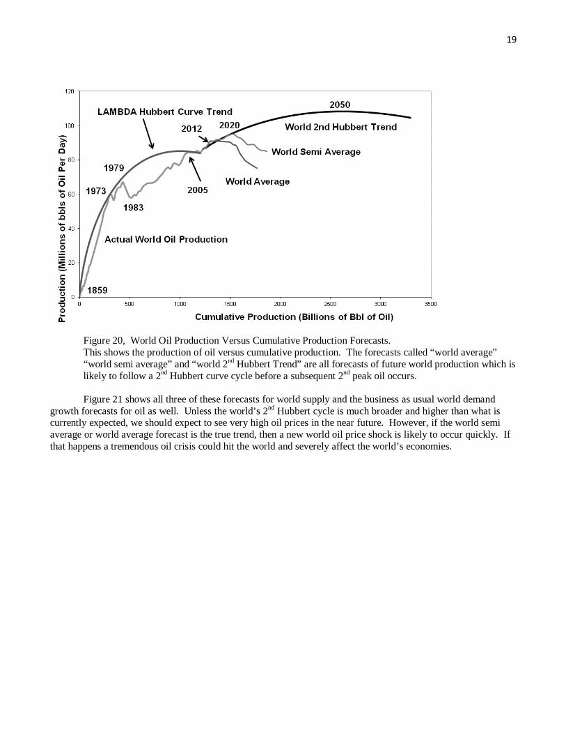
If we take an average of all the three 2nd cycles, together, we can calculate a world average expected 2nd cycle shown in figure 20 as the “world average” forecast. This may suggest a quick peak and decline for the world’s 2nd Hubbert cycle. If we take a weighted average of all three curves of figure 19, where the current world trend is counted at twice the weighted average as the US and former Soviet indexed curves, then we get what is called in Figure 20 the “world semi average”.

19

Figure 20, World Oil Production Versus Cumulative Production Forecasts. This shows the production of oil versus cumulative production. The forecasts called “world average” “world semi average” and “world 2nd Hubbert Trend” are all forecasts of future world production which is likely to follow a 2nd Hubbert curve cycle before a subsequent 2nd peak oil occurs. Figure 21 shows all three of these forecasts for world supply and the business as usual world demand

growth forecasts for oil as well. Unless the world’s 2nd Hubbert cycle is much broader and higher than what is currently expected, we should expect to see very high oil prices in the near future. However, if the world semi average or world average forecast is the true trend, then a new world oil price shock is likely to occur quickly. If that happens a tremendous oil crisis could hit the world and severely affect the world’s economies.

20

Figure 21, World Oil Production Versus Cumulative Production Forecasts. This shows the production of oil versus cumulative production. The forecasts called “world average” “world semi average” and “World 2nd Hubbert Trend” are all forecasts of future world production which is likely to follow a 2nd Hubbert curve cycle before a subsequent 2nd peak oil occurs. Also shown is the business as usual world growth trend.

8. Conclusion

The world growth rate since the financial crisis has been slower than the average growth rate for the previous ten years; however, that slow growth will still need robust oil supplies to keep it going. Therefore, the world’s economies are very dependent on oil, and so it is very important to consider how the supply of oil will change in the future. Indeed, the current lack of high world growth is as likely to be because of high oil prices as it is to be because of the financial crisis. After all, it is five years since the financial crisis was over and there has been no robust world growth rebound. On the other hand, average oil prices have remained very high and so those high prices may be causing the lack of robust world growth.

In this paper, we have tried to forecast the world’s oil production using the concept of the Lambda Hubbert curve and the concept of multi-cycle Hubbert curves. Before 2009, the world looked to be on a Lambda Hubbert curve trend, however, since 2009 there has been a new 2nd Hubbert cycle trend due to the shale oil and tar-sands phenomenon. This world 2nd Hubbert curve trend looks to be able to keep world oil production on a plateau with a slight increase all the way until 2005. However, if we look at other large oil production regions of the past, and compare them to the world’s current production cycle using an indexed curve, we see that there is a possibility of a much earlier peak than expected. If a quick peak and decline occur, then that would be very devastating to the world’s economies and we could see massive inflation and economic decline.

21 References Adelman, M.A. (1993). The Economics of Petroleum Supply, MIT Press, Cambridge. _____________ and M.C. Lynch (1997). "Fixed View of Resource Limits Creates Undue Pessimism," Oil and

Gas Journal, April 7, pp. 51 - 54. Al-Jarri, Abdulrahman S. and Richard A. Startzman (1999). "U.S. Oil Production and Energy Consumption: A

Hubbert Modeling Approach to Forecast Long Term Trends in Various Components of U.S. Energy Consumption with an Emphasis on Domestic Oil Production" in J.R. Moroney ed., Advances in the Economics of Energy and Resources, Volume 11, Fuels for the Future, JAI Press, Stamford, Connecticut, pp. 37 - 58.

Bardi, Ugo (2007). “Energy Prices and Resource Depletion: Lessons from the case of Whaling in the 19th Century. Energy Sources B: Economics planning and policy., 2: pp. 297–304.

___________, (2005). “The mineral economy: a model for the shape of oil production curves,” Energy Policy, Volume 33, Issue 1 , January 2005, Pages 53-61.

Brandt, Adam R. (2007). “Testing Hubbert,” in Energy Policy, Volume 35 pp. 3074-3088. Brandt, A. R., (2010). “Review of mathematical models of future oil supply: Historical overview and synthesizing

critique.” Energy 35 (9), 3958-3974. Campbell, Colin J., (2004). The Coming Oil Crisis, Multi-Science Publications Co. Ltd. London. ______________, and Jean H. Laherrere, (1998). “The End of Cheap Oil,” March Scientific American, pp. 78 -

83. Cleveland, Cutler J., (1991). Physical and Economic Aspects of Resource Quality, The Cost of Oil Supply in the

lower 48 United States, 1936 – 1988. Resources and Energy. 13: 163 - 188. _______________ and Robert K. Kaufmann, (1997). “Natural Gas in the U.S.: How Far Can Technology Stretch

the Resource Base?” The Energy Journal, vol. 18, no. 2, pp. 89-108. ______________ and Robert K. Kaufmann, (1991). Forecasting Ultimate Oil Resources and its Rate of

Production: Incorporating Economic Forces in the Models of M. King Hubbert. The Energy Journal. 12(2): 17 - 46.

Charness, Gary and Matthew O. Jackson (2009). “The Role of Responsibility in Strategic Risk-taking,” Journal of Economic Behavior & Organization, Volume 69, Issue 3, March 2009, Pages 241-247.

Federal Energy Administration (1974) Project Independence Report, Washington D.C. Hubbert, M.K. (1956). “Nuclear energy and fossil fuels,” American Petroleum Institute Drilling and Production

Practice Proceedings, Spring, pp. 7-25. ____________, (1962). Energy Resources, A Report to the Committee on Natural Resources: National Academy

of Sciences, National Research council, Publication 1000-D, Washington, D.C.. Kaufmann, Robert K. (1991). "Oil Production in the Lower 48 States: Reconciling Curve Fitting and Econometric

Models" Resources and Energy, Volume 13, pp. 111 - 127. ______________, Stephane Dees, Pavlos Karadeloglou, and Marcelo Sanchez, (2004). “Does OPEC Matter? An

Econometric Analysis of Oil Prices,” The Energy Journal, Vol. 25, no. 4, pp. 67-90. ______________, and Cutler Cleveland, (2001). “Oil Production in the Lower 48 States: Economic, Geological,

and Institutional Determinants,” The Energy Journal, vol. 21, no. 1, pp. 27-49. Loderer, Claudio (1985). “A Test of the OPEC Cartel Hypothesis: 1974-1983,” Journal of Finance, vol. 40, no. 3,

pp. 991-1008. Maugeri, Leonardo. (2004). “Oil: Never Cry Wolf—Why The Petroleum Age Is Far From Over.” Science, vol.

304, no. 21, May: pp. 1114 - 1115. Moroney, John R. and M. Douglas Berg (1999). “An Integrated Model of Oil Production,” The Energy Journal,

vol. 20, no. 1, pp. 105-124. Nehring, Richard. (2006a) “Two Basins Show Hubbert’s Method Underestimates Future Oil Production,” Oil and

Gas Journal, vol. 104, no. 13, pp. 37-44, 2006. Nehring, Richard. (2006b) “How Hubbert Method Fails to Predict Oil Production in the Permian Basin,” Oil and

Gas Journal, vol. 104, no. 15, pp. 30-35, 2006. Nehring, Richard. (2006c) “Post-Hubbert Challenge is to Find New Methods to Predict Production, EUR,” Oil

and Gas Journal, vol. 104, no. 16, pp. 43-51, 2006.

22 Newendorp, Paul, and John Schuyler (2000). Decision Analysis for Petroleum Exploration, 2nd Edition, Planning

Press, Aurora, Colorado. Norgaard, R.B., (1990). Economic Indicators of Resource Scarcity: A Critical Essay. Journal of Environmental

Economics and Management. 19(1): 19 - 25. Nystad, A.N. (1988). "On The Economics of Improved Oil Recovery: The Optimal Recovery Factor from Oil and

Gas Reservoirs," The Energy Journal, Vol 9, No. 4, October, pp 49 - 61. __________, (1987). "Rate Sensitivity and The Optimal Choice of Production Capacity of Petroleum Reservoirs,"

Energy Economics, Vol 9, No. 1, January, pp 37 - 45. Pesaran (1990). “An Econometric Analysis of Exploration and Extraction of Oil in the U.K. Continental Shelf,”

Economic Journal v100, number 4, (June), pp. 367-90. ____________, and H. Samiei (1995). "Forecasting Ultimate Resource Recovery,” International Journal of

Forecasting, Volume 11, Number 4, pp. 543 - 555. Pindyck, Robert S. (1978a). “Gains to Producers from the Cartelization of Exhaustible Resources,” Review of

Economic Statistices, 60(2), pp. 238 -251. _____________, (1978b). “The optimal exploration and production of Non renewable Resources,” Journal of

political Economy, 86(5): 841-861. Ramsey, J. (1980). Bidding and oil leases. Greenwich, CT: JAI Press. Reynolds, Douglas B. (2011a). Energy Civilization: The Zenith of Man, AlaskaChena Publishers, Fairbanks,

Alaksa. ______________. (2011b) “What Is OPEC? It Is Saudi Arabia,” in “OPEC at 50: Its Past, Present and Future in

a Carbon-constrained World,” March, 2011, conference proceedings, National Energy Policy Institute. _______________. (2009) Chapter 1, OIL SUPPLY DYNAMICS: HUBBERT, RISK AND INSTITUTIONS In:

OPEC, Oil Prices and LNG, Editor: Edward R. Pitt and Christopher N. Leung, ISBN:978-1-60692-897-4, ©2009 Nova Science Publishers,Inc.

_______________. (2002). Scarcity and Growth Considering Oil and Energy: An Alternative Neo-Classical View, The Edwin Mellen Press, 240 pages.

________________. (2001) “Oil Exploration Game with Incomplete Information: An Experimental Study,” Energy Sources, Volume 23, Number 6, July, pp. 571-578.

____________, (1999). “The Mineral Economy: How Prices and Costs Can Falsely Signal Decreasing Scarcity,” Ecological Economics, Volume 31, Number 1, pp. 155-166.

________________., Jacob Joseph, Reuben Sherwood (2009). “Risky Shift versus Cautious Shift: Determining differences in risk taking between private and public management decision-making,” in The Journal of Business & Economics Research, January 2009, volume 7 number 1.

__________________. and Michael K. Pippenger (2010). “OPEC and Venezuelan oil production: Evidence against a cartel hypothesis,” Energy Policy, 38, 6045-6055.

________________. and Yuanyuan Zhao (2007). "The Hubbert Curve and Institutional Changes: How Regulations in Alaska Created a U.S. Multi-Cycle Hubbert Curve," in The Journal of Energy and Development, Volume 32, Number 2, Spring 2007, pp. 159-186.

________________, and Jungho Baek (2012), “Much ado about Hotelling: beware the Ides of Hubbert,” Energy

Economics, 34 (2012), pp. 162-170. ________________, and Marek Kolodziej, (2009). “North American Natural Gas Supply Forecast: The Hubbert

Method Including the Effects of Institutions,” Energies 2009, 2(2), 269-306; doi:10.3390/en20200269 ________________, and Marek Kolodziej, (2008) “Former Soviet Union Oil Production and GDP Decline:

Granger Causality and the Multi-Cycle Hubbert Curve” Energy Economics. Volume 30, pp. 271-289. ________________, and Marek Kolodziej. (2007) “Institutions and The Supply of Oil: A Case Study of Russia”

Energy Policy, Volume 35, pp. 939 – 949. Richards, F.J., 1959. A Flexible Growth Curve for Empirical Use. Journal of Experimental Botany. 10: 290 -

300. Ryan, J.M. (2003). "Hubbert’s peak: Déjà vu All over Again," IAEE Newsletter, 2nd Quarter, pp. 9 - 12.

23 Simmons, Matthew (2005). Twilight in the Desert: The Coming Saudi Oil Shock and the World Economy , ISBN

0-471-73876-X. Smith, James L. (2005a) “Inscrutable OPEC? Behavior Tests of the Cartel Hypothesis,” The Energy Journal, vol.

26, no. 1, pp. 51-82. __________, (2005b). "Petroleum Prospect Valuation and the Option to Drill Again," The Energy Journal, vol.

26, no. 4, pp. 53 – 68. ____________ and James L. Paddock, (1984). Regional Modeling of Oil Discovery and Production. Energy

Economics 6(1): 5 - 13. Uhler, R.S., (1976). Costs and Supply in Petroleum Exploration: The Case of Alberta. Canadian Journal of

Economics. 9(1): 72 - 90. United States Energy Information Agency, EIA, (2005). International Energy Outlook, U.S. Department of

Energy, Energy Information Administration, at http://www.eia.doe.gov/. _______, (2004). “Mexico Country Analysis Brief,” at http://www.eia.doe.gov/emeu/cabs/mexico.pdf, November

2004. _______, (2000) “Long Term World Oil Supply,” EIA web site, EIA, 7/28/2000,

http://www.eia.doe.gov/pub/oil_gas/petroleum/presentations/2000/long_term_supply/index.htm. United States Geological Survey, USGS, (2000). U.S. Geological Survey World Peteroleum Assessment 2000 –

Description and Results, By USGS World Energy Assessment Team. Walls, Margaret A. (1992). "Modeling and Forecasting the Supply of Oil and Gas: A Survey of Existing

Approaches" Resources and Energy, Volume 14, pp. 287 - 309. Wiorkowski, J.J. (1981). "Estimating volumes of remaining fossil fuel resources: a critical review," Journal of the

American Statistical Association, Volume 76, Number 375, September, pp. 534 -547.