workshop 17 box beam with transient load …€¦ · zdatabase: open an existing msc.patran...
TRANSCRIPT
WS17-1PAT301, Workshop 17, December 2005Copyright© 2005 MSC.Software Corporation
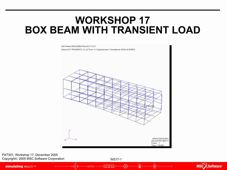
WORKSHOP 17BOX BEAM WITH TRANSIENT LOAD

WS17-2PAT301, Workshop 17, December 2005Copyright© 2005 MSC.Software Corporation

WS17-3PAT301, Workshop 17, December 2005Copyright© 2005 MSC.Software Corporation
Workshop ObjectivesPerform a modal analysis for a linear dynamic model. Also, perform a linear transient analysis for the model. View the shape of the model over time. Create an X vs Y plot of displacement vs time.
Problem DescriptionPerform modal and transient analysis of plate element modelCantilevered beam properties: include four concentrated massesTransient load on tip of cantilevered beam = constant tip force * function of time (f(t))
Software VersionMSC.Patran 2005r2MSC.Nastran 2005r2b

WS17-4PAT301, Workshop 17, December 2005Copyright© 2005 MSC.Software Corporation
Key Concepts and Steps:Database: open an existing MSC.Patran database for cantilevered beam with static loading at free end of beam.Elements: add four concentrated masses at free end of beamLoads/BCs: modify static loading to constant force * f(t)Properties: define the 0D elements as CONM2 elementsLoad Cases: create a time dependent fieldFields: create a non-spatial field for f(t)Analysis: Solution Type = Nastran Normal Modes, Solution Sequence = 103, Method = Full RunResults: display the deformed shape (mode shape) for some normal modesAnalysis: Solution Type = Nastran Transient Response, Solution Sequence = 112, Method = Full RunResults: display the structural shape over time, and displacement vs time for some nodes

WS17-5PAT301, Workshop 17, December 2005Copyright© 2005 MSC.Software Corporation
Step 1. Open Database cant_beam_transient.db
Open database.a. File / Open.b. Select cant_beam_transient.c. Click OK.
b
c
a
NOTE: warning message $# Journal file: …cant_beam_transient.db.jou does not exist is created. This is not a problem. A journal file does not exist for this database because one was not created when creating this database, i.e. File / Save a Copy has a toggle “Save Journal File Copy Also”.
WS17-6PAT301, Workshop 17, December 2005Copyright© 2005 MSC.Software Corporation
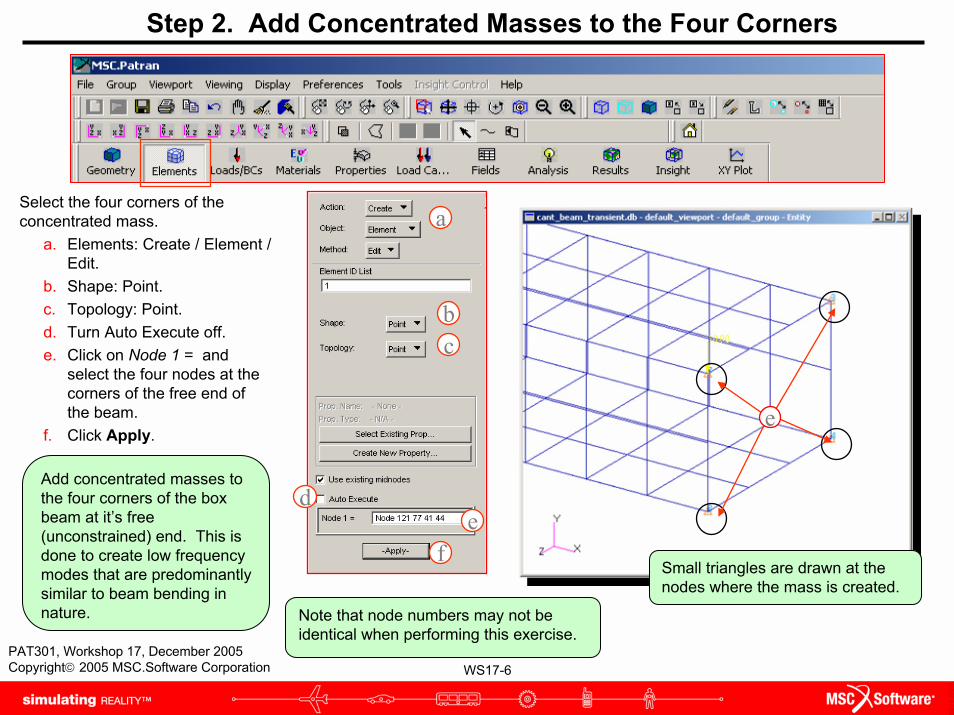
Step 2. Add Concentrated Masses to the Four Corners
Select the four corners of the concentrated mass.
a. Elements: Create / Element / Edit.
b. Shape: Point.c. Topology: Point.d. Turn Auto Execute off.e. Click on Node 1 = and
select the four nodes at the corners of the free end of the beam.
f. Click Apply.
Zoomeda
bc
e
Add concentrated masses to the four corners of the box beam at it’s free (unconstrained) end. This is done to create low frequency modes that are predominantly similar to beam bending in nature.
Small triangles are drawn at the nodes where the mass is created.
e
Note that node numbers may not be identical when performing this exercise.
d
f
WS17-7PAT301, Workshop 17, December 2005Copyright© 2005 MSC.Software Corporation
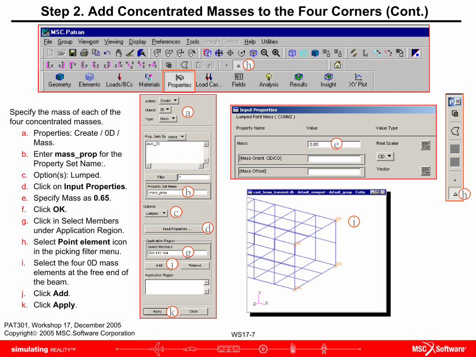
Step 2. Add Concentrated Masses to the Four Corners (Cont.)
Specify the mass of each of the four concentrated masses.
a. Properties: Create / 0D / Mass.
b. Enter mass_prop for the Property Set Name:.
c. Option(s): Lumped.d. Click on Input Properties.e. Specify Mass as 0.65.f. Click OK.g. Click in Select Members
under Application Region.h. Select Point element icon
in the picking filter menu.i. Select the four 0D mass
elements at the free end of the beam.
j. Click Add.k. Click Apply.
a
b
cd
e
g
h
i
j
k
h
WS17-8PAT301, Workshop 17, December 2005Copyright© 2005 MSC.Software Corporation
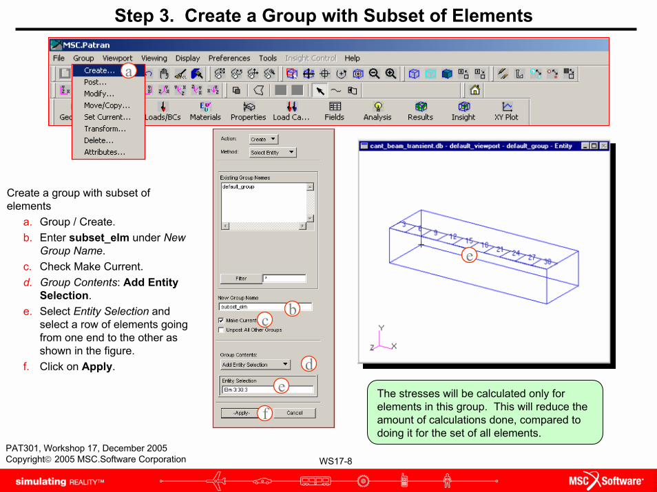
Step 3. Create a Group with Subset of Elements
Create a group with subset of elements
a. Group / Create.b. Enter subset_elm under New
Group Name.c. Check Make Current.d. Group Contents: Add Entity
Selection.e. Select Entity Selection and
select a row of elements going from one end to the other as shown in the figure.
f. Click on Apply.
a
bc
de
f
e
The stresses will be calculated only for elements in this group. This will reduce the amount of calculations done, compared to doing it for the set of all elements.

WS17-9PAT301, Workshop 17, December 2005Copyright© 2005 MSC.Software Corporation
Step 3. Create a Group with Subset of Elements (Cont.)
Include the nodes corresponding to elements in the group subset_elm
a. Tools / List / Create.b. Set the
Model/Object/Method to FEM/Node/Association.
c. Association: Element.d. Click on Target List: “A”.e. Select on Element and
select the same row of elements going from one end to the other just as done in the previous page.
f. Click on Apply.g. Add the list of nodes to the
group subset_elm by selecting Add to Group.
h. Click on Apply.
aThe list of nodes will be placed in the dialogue “List A”.
g
h
d
f
b
c
e

WS17-10PAT301, Workshop 17, December 2005Copyright© 2005 MSC.Software Corporation
Step 4. Post Group subset_elm
Post group subset_elm.a. Group / Post.b. Select subset_elm under
Select Groups to Post.c. Click on Apply.
a
b
c
WS17-11PAT301, Workshop 17, December 2005Copyright© 2005 MSC.Software Corporation
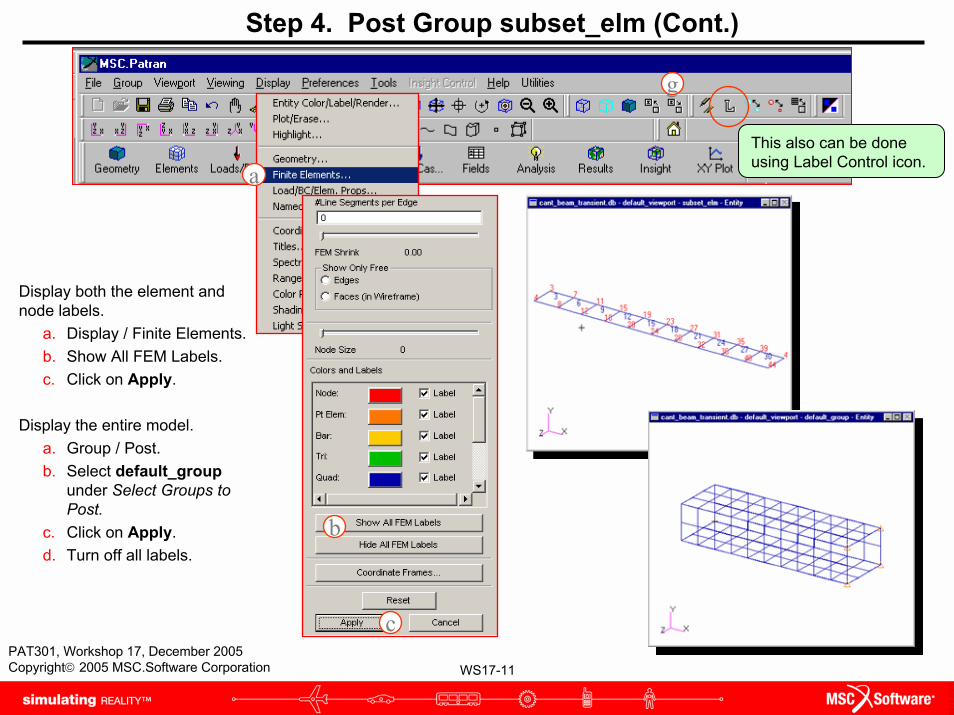
Step 4. Post Group subset_elm (Cont.)
Display both the element and node labels.
a. Display / Finite Elements.b. Show All FEM Labels.c. Click on Apply.
Display the entire model.a. Group / Post.b. Select default_group
under Select Groups to Post.
c. Click on Apply.d. Turn off all labels.
a
b
c
g
This also can be done using Label Control icon.
WS17-12PAT301, Workshop 17, December 2005Copyright© 2005 MSC.Software Corporation
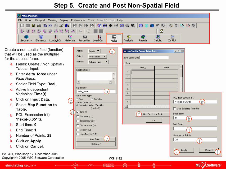
Step 5. Create and Post Non-Spatial Field
Create a non-spatial field (function) that will be used as the multiplier for the applied force.
a. Fields: Create / Non Spatial / Tabular Input.
b. Enter delta_force under Field Name.
c. Scalar Field Type: Real.d. Active Independent
Variables: Time(t).e. Click on Input Data.f. Select Map Function to
Table.g. PCL Expression f(‘t):
1*exp(-0.35*’t).h. Start time: 0.i. End Time: 1.j. Number of Points: 28.k. Click on Apply.l. Click on Cancel.
a
b
c
d
e
f
g
h
i
j
k l
WS17-13PAT301, Workshop 17, December 2005Copyright© 2005 MSC.Software Corporation
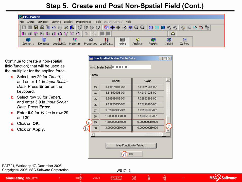
Step 5. Create and Post Non-Spatial Field (Cont.)
Continue to create a non-spatial field(function) that will be used as the multiplier for the applied force.
a. Select row 29 for Time(t), and enter 1.1 in Input Scalar Data. Press Enter on the keyboard.
b. Select row 30 for Time(t), and enter 3.0 in Input Scalar Data. Press Enter.
c. Enter 0.0 for Value in row 29 and 30.
d. Click on OK.e. Click on Apply.
d
cab

WS17-14PAT301, Workshop 17, December 2005Copyright© 2005 MSC.Software Corporation
Step 5. Create and Post Non-Spatial Field (Cont.)
a. Fields: Show.b. Select delta_force under
Select Field To Show. c. Select Specific Range.d. Minimum: 0.0.e. Maximum: 3.0.f. No. of Points: 30.g. OK.h. Check Post XY Plot. i. Click on Apply.
a
bd
c
e f
g
i
h
WS17-15PAT301, Workshop 17, December 2005Copyright© 2005 MSC.Software Corporation
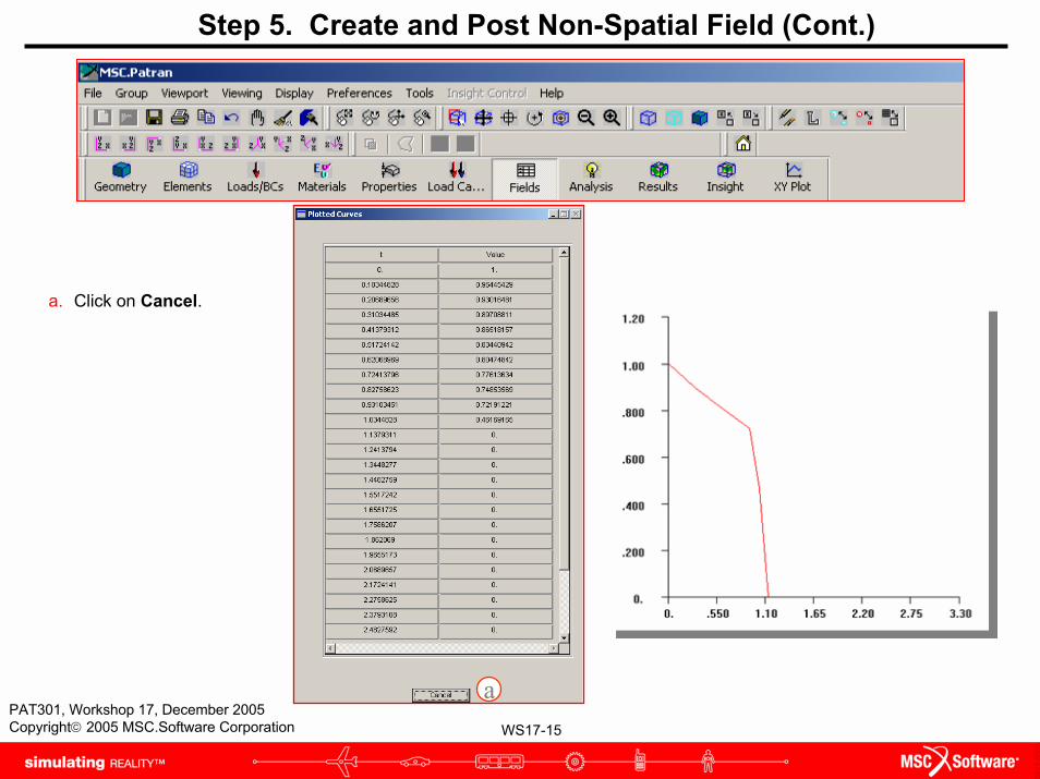
Step 5. Create and Post Non-Spatial Field (Cont.)
a. Click on Cancel.
a
WS17-16PAT301, Workshop 17, December 2005Copyright© 2005 MSC.Software Corporation
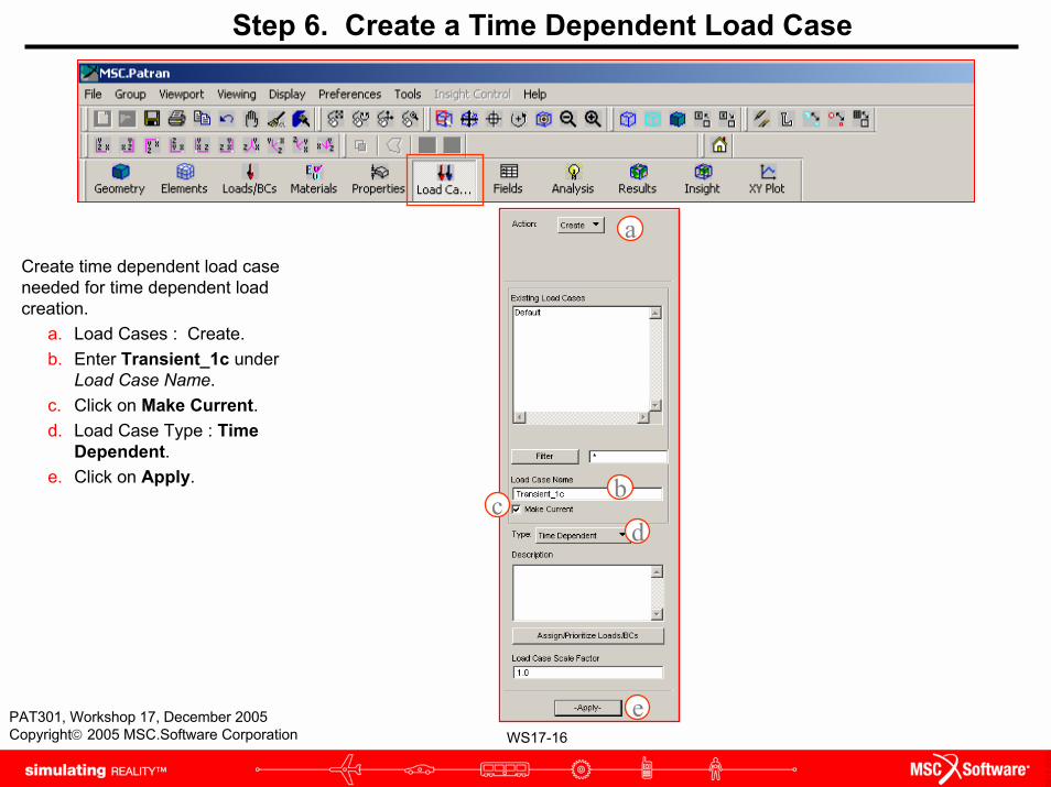
Step 6. Create a Time Dependent Load Case
Create time dependent load case needed for time dependent load creation.
a. Load Cases : Create.b. Enter Transient_1c under
Load Case Name.c. Click on Make Current.d. Load Case Type : Time
Dependent.e. Click on Apply.
a
bc
d
e

WS17-17PAT301, Workshop 17, December 2005Copyright© 2005 MSC.Software Corporation
Step 7. Modify the Applied Force
Modify the force to include t (time).a. Loads/BCs: Modify / Force /
Nodal.b. Current Load Case:
Transient_1c. (Type: Time Dependent)
c. Select force under Select Set to Modify.
d. Modify Data.e. Change <0 –10 0> to
<0 –10000 0> in Force <F1 F2 F3>.
f. Click in * Time/Freq. Dependence and select delta_force under Time/Freq. Dependent Fields.
g. Click on OK.h. Click on Apply.
a
b
c
d
f
gh
e
f
NOTE: the spatial and time dependent functions are multiplied, e.g. <0 –10000 0> * f:delta_force. Make sure that force is assigned to Load Case Transient_1c.
WS17-18PAT301, Workshop 17, December 2005Copyright© 2005 MSC.Software Corporation
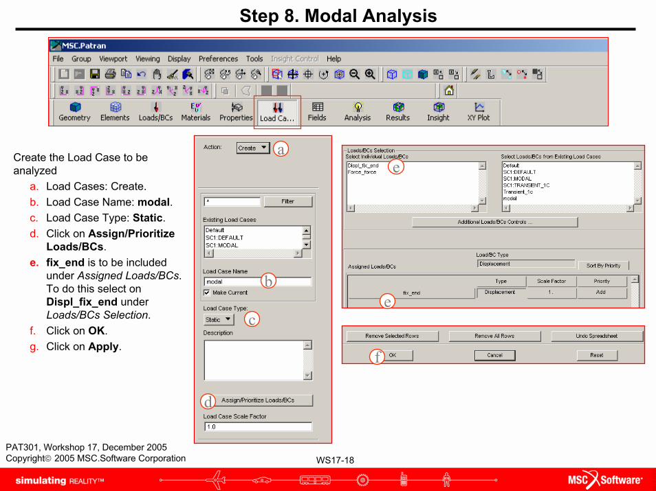
Step 8. Modal Analysis
Create the Load Case to be analyzed
a. Load Cases: Create.b. Load Case Name: modal.c. Load Case Type: Static.d. Click on Assign/Prioritize
Loads/BCs.e. fix_end is to be included
under Assigned Loads/BCs. To do this select on Displ_fix_end under Loads/BCs Selection.
f. Click on OK.g. Click on Apply.
a
b
c
d
f
e
e
WS17-19PAT301, Workshop 17, December 2005Copyright© 2005 MSC.Software Corporation
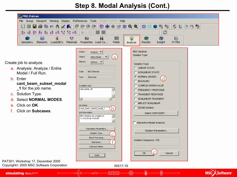
Step 8. Modal Analysis (Cont.)
Create job to analyze.a. Analysis: Analyze / Entire
Model / Full Run.b. Enter
cant_beam_subset_modal_1 for the job name.
c. Solution Type.d. Select NORMAL MODES.e. Click on OK.f. Click on Subcases.
a
b
c
d
e
f

WS17-20PAT301, Workshop 17, December 2005Copyright© 2005 MSC.Software Corporation
Step 8. Modal Analysis (Cont.)
Continue to create the job for the modal analysis.
a. Select modal under Available Subcases.
b. Select modal under Available Load Cases.
c. Subcase Parameters.d. Extraction Method: Lanczos.e. Lower = 0.0(Hz).f. Upper = 100.0(Hz).g. Click on OK.h. Click on Apply.i. Click on Cancel.
a
b
d
ef
g
h
c
i

WS17-21PAT301, Workshop 17, December 2005Copyright© 2005 MSC.Software Corporation
Step 8. Modal Analysis (Cont.)
Run the modal analysis.a. Subcase Select...b. Select modal under
Subcases For Solution Sequence: 103. Make sure only modal appears under Subcases Selected.
c. Click on OK.d. Click on Apply. This will run
the modal analysis.
a
b
c
b
d

WS17-22PAT301, Workshop 17, December 2005Copyright© 2005 MSC.Software Corporation
Step 8. Modal Analysis (Cont.)
Attach XDB File.a. Analysis: Access Results /
Attach XDB / Result Entities.b. Click on Select Results
File.c. Select and attach the file
cant_beam_subset_modal_1.xdb.
d. Click on OK.e. Click on Apply.
a
b
c
d
e

WS17-23PAT301, Workshop 17, December 2005Copyright© 2005 MSC.Software Corporation
Step 8. Modal Analysis (Cont.)
Create deformation display for the first mode.
a. Results: Create / Deformation.
b. Select MODAL, A2:Mode 1:Freq.=13.441 under Select Result Case(s).
c. Select Eigenvectors, Translational under Select Deformation Result.
d. Show As: Resultant.e. Click on Apply.
a
b
c
d

WS17-24PAT301, Workshop 17, December 2005Copyright© 2005 MSC.Software Corporation
Step 8. Modal Analysis (Cont.)
Create deformation display for other modes.
a. Select MODAL, A2:Mode 2:Freq.=17.879 under Select Result Case(s).
b. Click on Apply.c. Select MODAL,
A2:Mode 3:Freq.=21.082 under Select Result Case(s).
d. Click on Apply.
WS17-25PAT301, Workshop 17, December 2005Copyright© 2005 MSC.Software Corporation
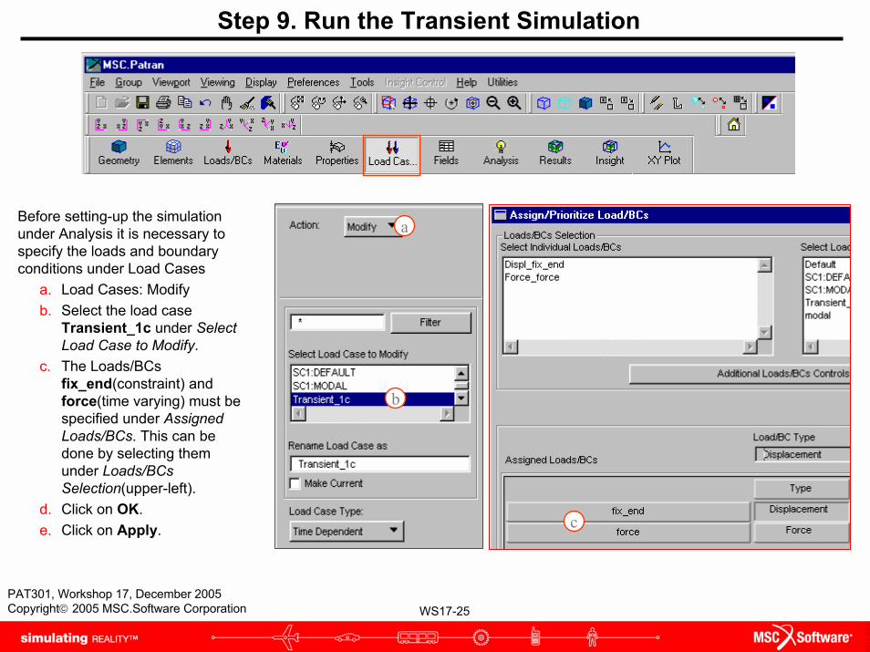
Step 9. Run the Transient Simulation
Before setting-up the simulation under Analysis it is necessary to specify the loads and boundary conditions under Load Cases
a. Load Cases: Modifyb. Select the load case
Transient_1c under Select Load Case to Modify.
c. The Loads/BCsfix_end(constraint) and force(time varying) must be specified under Assigned Loads/BCs. This can be done by selecting them under Loads/BCsSelection(upper-left).
d. Click on OK.e. Click on Apply.
a
b
c

WS17-26PAT301, Workshop 17, December 2005Copyright© 2005 MSC.Software Corporation
Step 9. Run the Transient Simulation (Cont.)
Run the Transient Simulation.a. Analysis: Analyze / Entire
Model / Full Run.b. Enter Job Name
cant_beam_subset_elmc. Select Solution Type.d. Choose TRANSIENT
RESPONSE for Solution Type.e. Formulation: Modal.f. Click on Solution
Parameters.g. Eigenvalue Extraction.h. Extraction Method: Lanczos.i. Lower = 0.0 (Hz).j. Upper = 100.0 (Hz).k. Number of Desired Roots = 10.l. Click on OK.m. Click on OK.n. Click on OK.
b
c
d
ef
g
h
ij
k
lm
a
WS17-27PAT301, Workshop 17, December 2005Copyright© 2005 MSC.Software Corporation
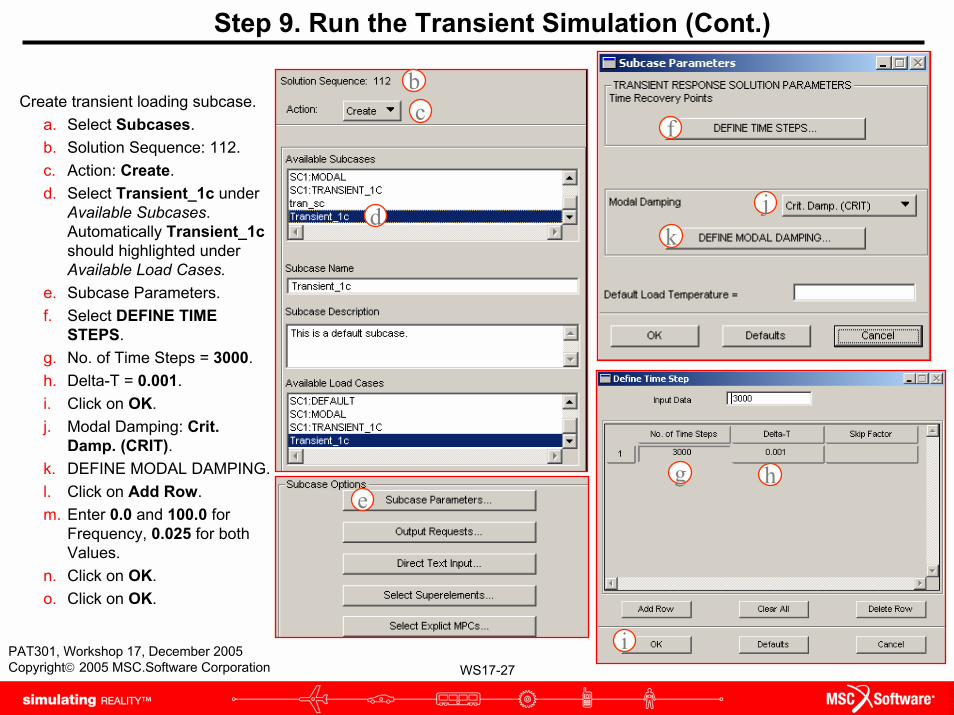
Step 9. Run the Transient Simulation (Cont.)
Create transient loading subcase.a. Select Subcases.b. Solution Sequence: 112.c. Action: Create.d. Select Transient_1c under
Available Subcases. Automatically Transient_1c should highlighted under Available Load Cases.
e. Subcase Parameters.f. Select DEFINE TIME
STEPS.g. No. of Time Steps = 3000.h. Delta-T = 0.001.i. Click on OK.j. Modal Damping: Crit.
Damp. (CRIT).k. DEFINE MODAL DAMPING.l. Click on Add Row.m. Enter 0.0 and 100.0 for
Frequency, 0.025 for both Values.
n. Click on OK.o. Click on OK.
bc
d
e
f
g h
i
jk
WS17-28PAT301, Workshop 17, December 2005Copyright© 2005 MSC.Software Corporation
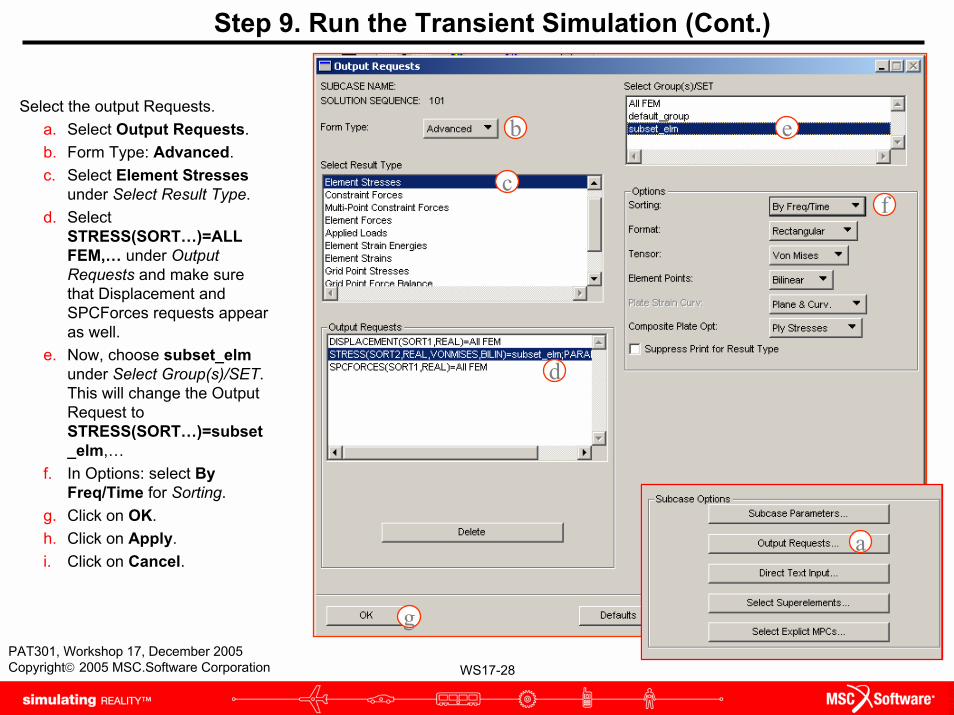
Step 9. Run the Transient Simulation (Cont.)
Select the output Requests.a. Select Output Requests.b. Form Type: Advanced.c. Select Element Stresses
under Select Result Type.d. Select
STRESS(SORT…)=ALL FEM,… under Output Requests and make sure that Displacement and SPCForces requests appear as well.
e. Now, choose subset_elmunder Select Group(s)/SET. This will change the Output Request to STRESS(SORT…)=subset_elm,…
f. In Options: select By Freq/Time for Sorting.
g. Click on OK.h. Click on Apply.i. Click on Cancel.
b
c
d
e
f
g
a

WS17-29PAT301, Workshop 17, December 2005Copyright© 2005 MSC.Software Corporation
Step 9. Run the Transient Simulation (Cont.)
Select Subcase.a. Select Subcase Select.b. Under Subcases Selected,
only the desired subcase, Transient_1c should appear. This can be achieved by selecting names in the upper and lower boxes.
c. Click on OK.d. Click on Apply.
a
b
c
d

WS17-30PAT301, Workshop 17, December 2005Copyright© 2005 MSC.Software Corporation
Step 10. Access Results Under Analysis
Attach transient results XDB file.a. Analysis : Access Results /
Attach XDB / Result Entities.b. Click on Select Results File.c. Select and attach the file
cant_beam_subset_elm.xdb.d. Click on OK.e. Click on Apply.
a
c
d
b
e

WS17-31PAT301, Workshop 17, December 2005Copyright© 2005 MSC.Software Corporation
Step 11. View the Transient Deformation Results
View time dependent deformation results at a single time.
a. Results : Create / Deformation.
b. Click on the View Subcases icon.
c. Select TRANSIENT…Time=0.154under Select Result Case(s).
d. Select Displacements, Translational under Select Deformation Result.
e. Show As: Resultant.f. Click on Apply.g. Show As: Component.h. Select YY only.i. Click on Apply.j. Look at other individual
times.The title in the upper left corner of the viewport gives the time and result type.
a
c
d
b
e

WS17-32PAT301, Workshop 17, December 2005Copyright© 2005 MSC.Software Corporation
Step 11. View the Transient Deformation Results (Cont.)
Next, look at how the model deforms with time.
a. Results: Create / Deformation.b. For the View Subcases icon
not depressed, select all the transient subcases under Select Result Case(s) using the shift key. Or, can select all or a subset of the transient result cases by selecting the View Subcases icon (see next page).
c. Select Displacements, Translational under Select Deformation Result.
d. Show As: Resultant.e. Check Animate.f. Select Animation Options.
a
b
f
c
View Subcases
d
e
WS17-33PAT301, Workshop 17, December 2005Copyright© 2005 MSC.Software Corporation
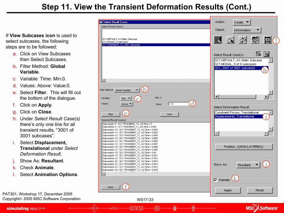
If View Subcases icon is used to select subcases, the following steps are to be followed:
a. Click on View Subcases then Select Subcases.
b. Filter Method: Global Variable.
c. Variable: Time: Min:0.d. Values: Above: Value:0.e. Select Filter. This will fill out
the bottom of the dialogue.f. Click on Apply.g. Click on Close.h. Under Select Result Case(s)
there’s only one line for all transient results, “3001 of 3001 subcases”.
i. Select Displacement, Translational under Select Deformation Result.
j. Show As: Resultant.k. Check Animate.l. Select Animation Options.
Step 11. View the Transient Deformation Results (Cont.)
bc
de
f
h
i
j
k
l
WS17-34PAT301, Workshop 17, December 2005Copyright© 2005 MSC.Software Corporation
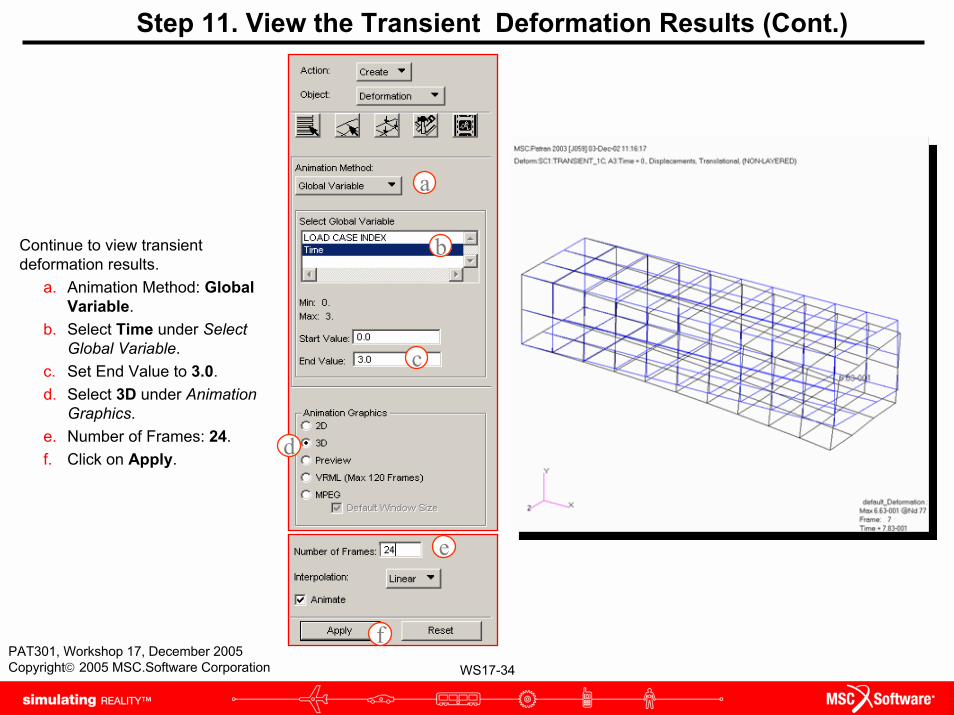
Step 11. View the Transient Deformation Results (Cont.)
Continue to view transient deformation results.
a. Animation Method: Global Variable.
b. Select Time under Select Global Variable.
c. Set End Value to 3.0.d. Select 3D under Animation
Graphics.e. Number of Frames: 24.f. Click on Apply.
a
b
d
e
f
c
WS17-35PAT301, Workshop 17, December 2005Copyright© 2005 MSC.Software Corporation
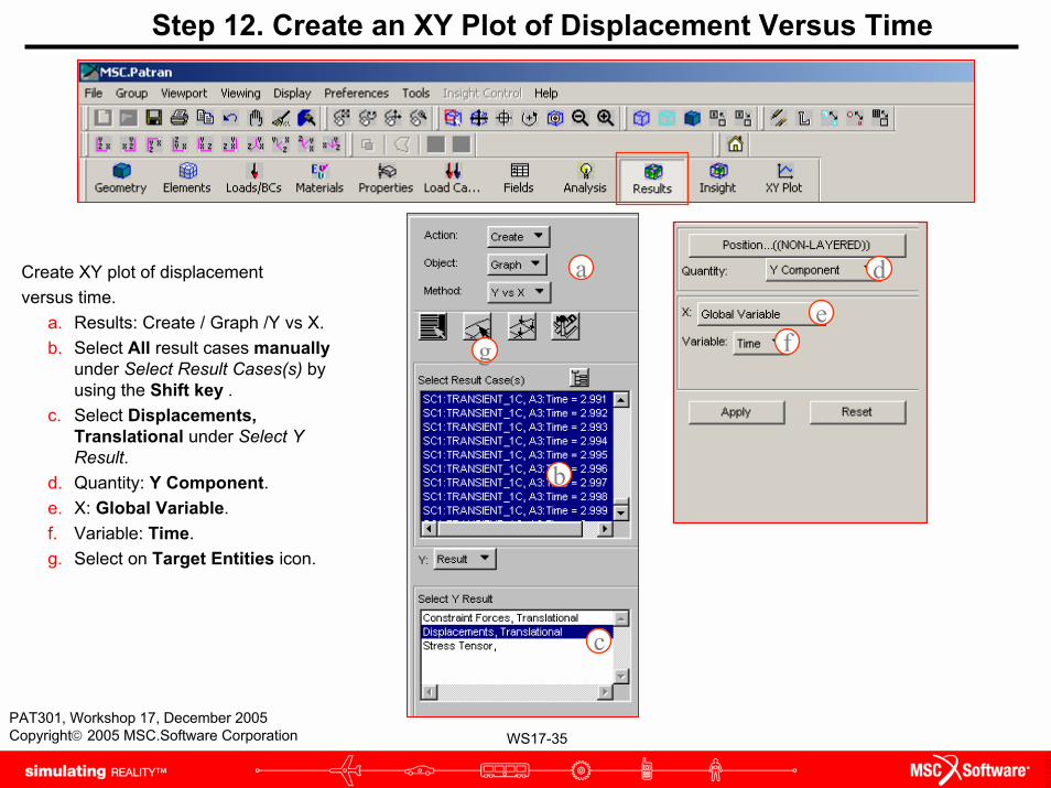
Step 12. Create an XY Plot of Displacement Versus Time
Create XY plot of displacementversus time.
a. Results: Create / Graph /Y vs X.b. Select All result cases manually
under Select Result Cases(s) by using the Shift key .
c. Select Displacements, Translational under Select Y Result.
d. Quantity: Y Component.e. X: Global Variable.f. Variable: Time.g. Select on Target Entities icon.
a
b
c
d
efg

WS17-36PAT301, Workshop 17, December 2005Copyright© 2005 MSC.Software Corporation
Step 12. Create an XY Plot of Displacement Versus Time (Cont.)
Continue to create an XY plot of displacement versus time.
a. Reset the graphics to un-display any results
b. Target Entity: Nodes. c. Select Nodes: Click on the
top corner node as shown in the figure.
d. Click on Apply.b
c
d
a
c

WS17-37PAT301, Workshop 17, December 2005Copyright© 2005 MSC.Software Corporation
Step 12. Create an XY Plot of Displacement Versus Time (Cont.)
View resulting plot.a. The plot should look like the
following.
The XY plot is created for one displacement, Node 44 Y-component. Notice that the displacement follows the applied force.

WS17-38PAT301, Workshop 17, December 2005Copyright© 2005 MSC.Software Corporation
Step 12. Create an XY Plot of Displacement Versus Time (Cont.)
Create another XY plota. Add another XY plot by
selecting the node shown in the figure.
The XY plot is created for two displacements.
WS17-39PAT301, Workshop 17, December 2005Copyright© 2005 MSC.Software Corporation
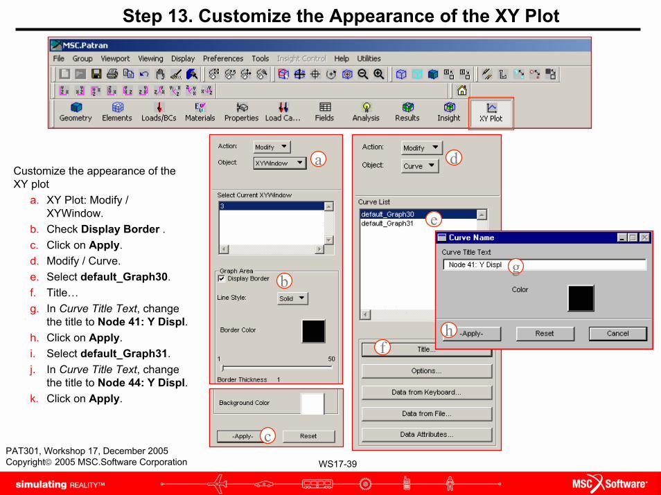
Step 13. Customize the Appearance of the XY Plot
Customize the appearance of the XY plot
a. XY Plot: Modify / XYWindow.
b. Check Display Border .c. Click on Apply.d. Modify / Curve.e. Select default_Graph30.f. Title…g. In Curve Title Text, change
the title to Node 41: Y Displ.h. Click on Apply.i. Select default_Graph31.j. In Curve Title Text, change
the title to Node 44: Y Displ.k. Click on Apply.
a
b
c
d
e
f
g
h

WS17-40PAT301, Workshop 17, December 2005Copyright© 2005 MSC.Software Corporation
Step 13. Customize the Appearance of the XY Plot (Cont.)
Continue to customize the appearance of the XY plot.
a. XY Plot: Create / Title.b. Title: Displ vs. Time .c. Change X Alignment to
Percent(%) and set X Location (%): 39.
d. Y Location (%): 14.e. Font Size: 18.f. Click on Apply.g. Modify / Legend.h. Title: ND.i. Click on Apply.
a
b
c
d
ef
g
h
i

WS17-41PAT301, Workshop 17, December 2005Copyright© 2005 MSC.Software Corporation
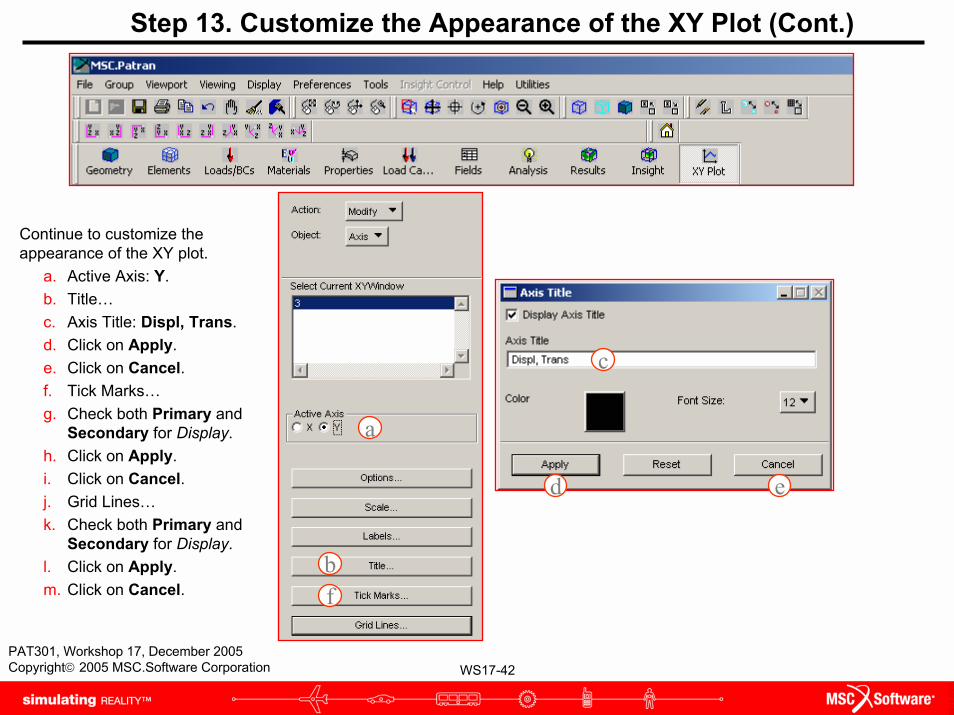
Step 13. Customize the Appearance of the XY Plot (Cont.)
Continue to customize the appearance of the XY plot
a. Modify / Axis.b. Active Axis: X.c. Scale…d. Assignment Method: Range.e. Enter 0.0, 3.0 for Lower and Upper
Values.f. Enter 10 for Number of Primary Tick
Marks.g. Click on Apply.h. Click on Cancel.i. Tick Marks…j. Check both Primary and Secondary
for Display.k. Click on Apply.l. Click on Cancel.m. Grid Lines…n. Check both Primary and Secondary
for Display.o. Click on Apply.p. Click on Cancel.
a
b
c
d
e
f
g h
i
j
k l
m
WS17-42PAT301, Workshop 17, December 2005Copyright© 2005 MSC.Software Corporation
Step 13. Customize the Appearance of the XY Plot (Cont.)
Continue to customize the appearance of the XY plot.
a. Active Axis: Y.b. Title…c. Axis Title: Displ, Trans.d. Click on Apply.e. Click on Cancel.f. Tick Marks…g. Check both Primary and
Secondary for Display.h. Click on Apply.i. Click on Cancel.j. Grid Lines…k. Check both Primary and
Secondary for Display.l. Click on Apply.m. Click on Cancel.
a
b
c
d e
f
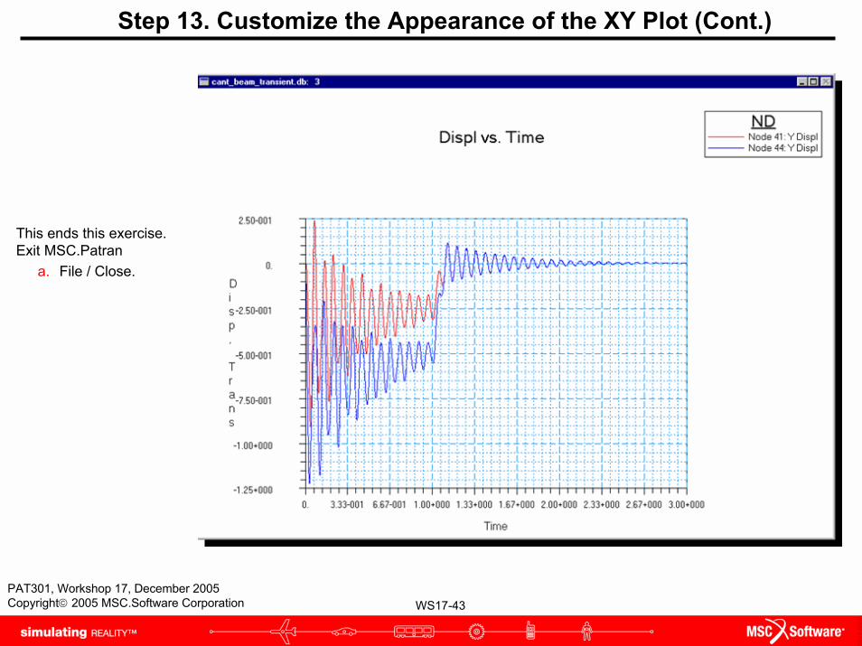
WS17-43PAT301, Workshop 17, December 2005Copyright© 2005 MSC.Software Corporation
This ends this exercise. Exit MSC.Patran
a. File / Close.
Step 13. Customize the Appearance of the XY Plot (Cont.)
WS17-44PAT301, Workshop 17, December 2005Copyright© 2005 MSC.Software Corporation