workman & niswander (1970)

Population Studies on Southwestern Indian Tribes.II. Local Genetic Differentiation in the Papago

P. L. WORKMAN1 AND J. D. NISWANDER'

INTRODUCTION

In a previous publication we have described the ethnohistory and demography ofthe Papago Indians of southwestern Arizona (Niswander et al. 1970). During thereview of the relevant anthropological studies it became apparent that the Papagodo not conform to a model of a homogeneous population within which mating occursat random. On the Papago reservation there are about 5,000 Indians distributedamong geographically distinct villages or clusters of villages. Approximately 60%oof the Indians live in the 10 largest villages. The village groups are of two types.Most consist of villages derived from a single ancestral village, the so-called defensevillage founded in the seventeenth century as a means of protection against attacksby the Apache Indians. Some villages (e.g., Sells) or groups of villages (e.g., the SanXavier district) appear to have been populated largely by immigrants from otherparts of the reservation during the past 75 years. Studies on the mating patternsshow considerable endogamy not only within regions but also within individualvillages. Thus the Papago appear to approximate a model of a population comprisinga small number of partially isolated subpopulations.

Subdivided populations may be said to conform to one of three basic models:hierarchical, island, or stepping-stone (see Yasuda and Morton 1967). Since there isinsufficient information on the historical relations among the founders of the Papagovillage groups and no evidence that migrants to each group are representative ofthe total population, neither the hierarchical nor the island model is appropriate.The stepping-stone model (Kimura and Weiss 1964; Bodmer and Cavalli-Sforza1968), which requires only the assumption of discrete subdivisions among whichthere is migration, appears to provide the most realistic approximation to Papagopopulation structure. When the subgroups are partially isolated, such factors asrandom genetic drift and isolation by distance may result in significant geneticdifferentiation among groups. A large sample of the Papago population has beencharacterized in terms of blood groups and serum protein genotypes (Niswanderet al. 1970), and in this paper we shall use these results to analyze the genetic struc-ture of the Papago population.We shall first examine the pattern of genetic variation among groups, using both

x2 tests and F statistics analyses developed by Wright (1943a, 1951, 1965) and Nei

Received May 26, 1969.1 Human Genetics Branch, National Institute of Dental Research, National Institutes of Health,

Bethesda, Maryland 20014.© 1970 by the American Society of Human Genetics. All rights reserved.

24

GENETIC DIFFERENTIATION IN THE PAPAGO

(1965). Utilizing demographic, geographic, and historical information, we shall at-tempt to determine the factors responsible for the particular pattern of variationobserved. Finally, comparisons with other small subdivided populations will provide abasis for general comments on local differentiation in populations with a stepping-stone type of structure.

GENETIC DATA

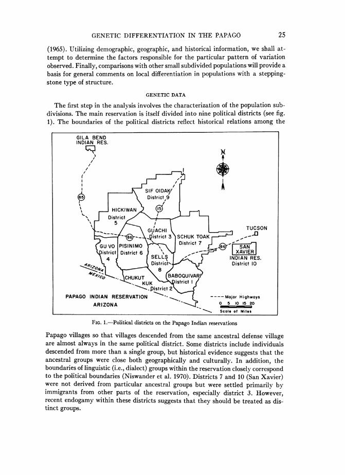
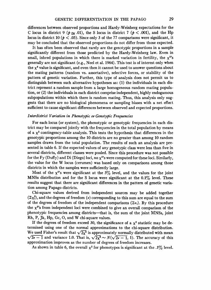
The first step in the analysis involves the characterization of the population sub-divisions. The main reservation is itself divided into nine political districts (see fig.1). The boundaries of the political districts reflect historical relations among the

PAP

GILA BENDINDIAN RES.

/)

¢)\ ~~~~~~District 9

/

str ict<

5

TUCSON

i=:j .\^Iistrict 3 SCHUK TOAK

fGUVO |PISINIMO A n iDistrict 7 - SAN

strict District 6 XAVIER

> \A K~~Distit ric District 10

.. KUK\ itrict 1IX'-<Distri t2

'AGO INDIAN RESERVATION ' ----Major HighwaysARIZONA : °S o Miles

Scale of Miles

FIG. 1.-Political districts on the Papago Indian reservations

Papago villages so that villages descended from the same ancestral defense villageare almost always in the same political district. Some districts include individualsdescended from more than a single group, but historical evidence suggests that theancestral groups were close both geographically and culturally. In addition, theboundaries of linguistic (i.e., dialect) groups within the reservation closely correspondto the political boundaries (Niswander et al. 1970). Districts 7 and 10 (San Xavier)were not derived from particular ancestral groups but were settled primarily byimmigrants from other parts of the reservation, especially district 3. However,recent endogamy within these districts suggests that they should be treated as dis-tinct groups.

25

26 WORKMAN AND NISWVANDER

The use of political districts reflects both historic and contemporary relationsamong villages. An alternative subdivision based on Jones's (1969) description of thehistoric relations among villages (especially during the nineteenth century) was alsoexamined. The resulting subgroups were essentially the same as those based onpolitical districts, and a partial analysis of the alternative grouping yielded resultsvery similar to those which will be considered in this paper.

The foregoing observations justify the description of the Papago population understudy as one comprising 10 partially isolated subpopulations, each corresponding to asingle political district. Limitations of sample sizes prevented further subdivision of

TABLE 1

A COMPARISON OF THE POPULATION SAMPLE WITH THE TOTALPAPAGO POPULATION BY POLITICAL DISTRICTS

PAPAGO POPULATIONS-1967 CENSUS* SAMPLE INDIVIDUAL

DISTRICT _______________________ OVER4 YEARS OLD

N % of N % of Total (N)Total Sample

1 ......... 621 12.1 71 10.4 13.62 ......... 126 2.5 29 4.3 27.43. 538 10.5 80 11.7 16.94 ......... 287 5.6 48 7.0 18.45 ......... 353 6.7 55 8.1 17.76 ......... 398 7.9 28 4.1 8.37 ......... 291 5.7 68 10.0 19.08 ......... 1,333 26.3 191 28.0 16.79 ......... 597 11.8 51 7.5 10.010 ............ 558 11.0 60 8.8 12.2

Total........ 5,102 100.0 681 100. 0 15.4

* Data from Division of Indian Health, Tucson, Arizona.

the population in terms either of individual villages of or clusters descended from asingle ancestral group.

In order that comparisons among districts be independent of sample size, it isessential that the sample size in each district be proportional to the total populationin the district. The composition of the Papago sample is shown in table 1. Althoughthe actual sample sizes vary considerably, they correspond closely to the actual pro-portions in each district. Genetic data were provided only by individuals over fouryears old, and the sample includes 15%7 of the Papago in that age category.

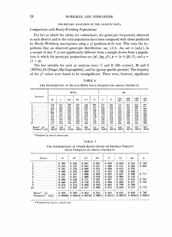
As reported by Niswander et al. (1970), genetic information was obtained from714 individuals who could be described as full-blooded Indian. For 681 of these,village or district of residence was determined using either the Papago PopulationRegister (see discussion in Niswander et al. 1970) or other sources of informationsuch as school records, interviews, etc. The blood group and protein phenotypes ofthese individuals are given by district in tables 2 and 3. The corresponding genefrequencies are given in tables 4 and 5.

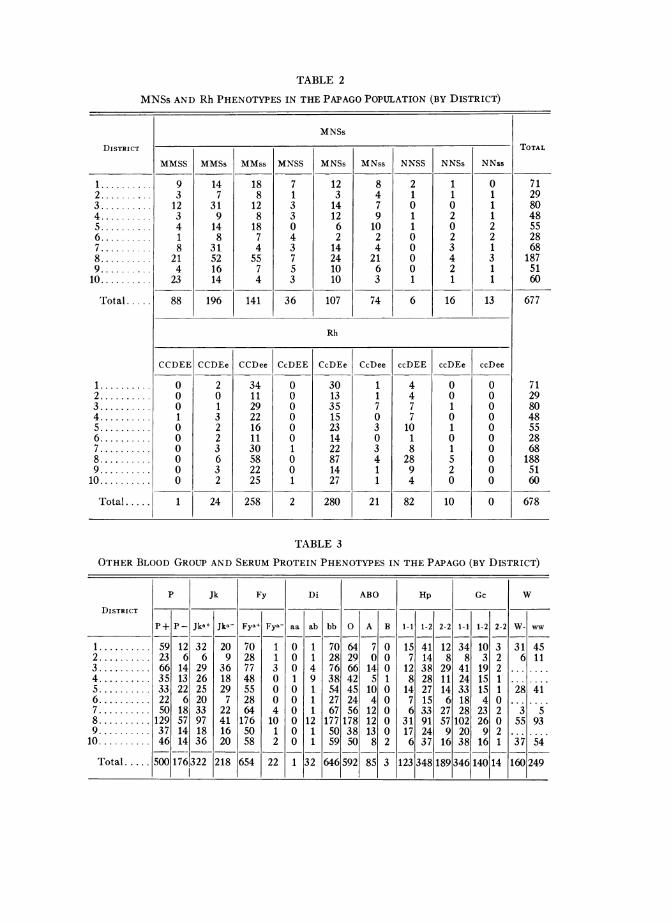
TABLE 2

MNSS AND Rh PHENOTYPES IN THE PAPAGO POPULATION (BY DISTRICT)

DISTRICT

1..........

2..........3..........4..........5..........6..........7..........8..........9..........10..........

Total ....

1..........2..........3..........4..........5..........6..........7..........8..........9..........10..........

Total .....

MNSs

MMSS

93123418

214

23

88

IMMSs147

319148

31521614

196

MMss

188

12818745574

141

MNSS

71330

4375

3

36

MNSs

12314126214241010

107

MNss

847910242163

NNSS

210

110

0

0

0

1

NNSs

1

0

20

23421

NNss

0

11

1

22

1

3

1

1

_ I74 6 16 13

Rh

CCDEE CCDEe CCDee CcDEE CcDEe CcDee ccDEE ccDEe ccDee

0

0

0

10

0

0

0

0

0

1

20

13223632

24

34112922161130582225

258

0

0

0

0

0

0

10

0

1

2

30133515231422871427

280

1

1

70

30

3411

21

4477

1018

2894

82

0

0

10

10

15

20

10

0

0

0

0

0

0

0

0

0

0

0

TOTAL

71298048552868

1875160

677

712980485528681885160

678

TABLE 3

OTHER BLOOD GROUP AND SERUM PROTEIN PHENOTYPES IN THE PAPAGO (BY DISTRICT)

P Jk Fy Di ABO Hp Gc W

DiSTRICT

P+ P- Jk,, jka- Fy| Fya- aa ab bb 0 A B 1-1 1-2 2-2 1-1 1-2 2-2 W- ww

1.......... 59 12 32 20 70 1 0 1 70 64 7 0 15 41 12 34 10 3 31 452........ 23 6 6 9 28 1 0 1 28 29 0 0 7 14 8 8 3 2 6 113........ 66 14 29 36 77 3 0 4 76 66 14 0 12 38 29 41 19 2 .......4.......... 35 13 26 18 48 0 1 9 38 42 5 1 8 28 11 24 15 1 ... ....

5........ 33 22 25 29 55 0 0 1 54 45 10 0 14 27 14 33 15 1 28 416........ 22 6 20 7 28 0 0 1 27 24 4 0 7 15 6 18 4 0 .......

7........ 50 18 33 22 64 4 0 1 67 56 12 0 6 33 27 28 23 2 3 58.1. 29 57 97 41 176 10 0 12 177 178 12 0 31 91 57 102 26 0 55 939. 37 14 18 16 5 1 00 1 50 38 13 0 17 24 9 20 9 2 ...

10 .......... 46 14 36 20 58 2 0 1 59 50 8 2 6 37 16 38 16 1 37 54

Total... 500 176322 218 654 22 1 32 646592 85 3 12334818934614014 160 249

l~1-- 1 - -

28 WORKMAN AND NISWANDER

CHI-SQUARE ANALYSES OF THE GENETIC DATA

Comparisons with Hardy-Weinberg Expectations

For loci at which the alleles are codominant, the genotypic frequencies observedin each district and in the total population have been compared with those predictedby Hardy-Weinberg assumptions using a x2 goodness-of-fit test. This tests the hy-pothesis that an observed genotypic distribution, say (AA, Aa, aa) = (a,b,c), ina sample of size N, is not significantly different from a sample drawn from a popula-tion in which the genotypic proportions are (p2, 2pq, q2); p = (a + 'b)/N; and q =(t-p).The loci suitable for such an analysis were: C and E (Rh system), M and S

(MNSs),Di (Diego),Hp (haptoglobin), and Gc (group-specific protein). The majorityof the x2 values were found to be nonsignificant. There were, however, significant

TABLE 4

THE DISTRIBUTION OF Rh AND MNSs GENE FREQUENCIES AMONG DISTRICTS

MNSs Rh

DISTRICT

M S Ms Ms NS NS C E ~~CDe cDE CDE cDeDISM t S M.S Ms NS .Vs 1 C E (RI) (R2) (Rz) (Je)I ........... .768 .443 .300 .470 .146 .086 725 .282 .711 .267 .014 .0072............ .759 .362 .264 .495 .098 .143 .621 .362 .621 .362 .000 .0173............ .838 .469 .430 .408 .039 .124 .638 .319 .631 .312 007 .0504............ .667 .385 .240 .426 .145 .188 .698 354 .646 .302 .052 .0005............ .800 .273 .235 .565 .038 .162 .564 .418 .545 .399 .019 .0376............ .714 .393 .265 .449 .128 .158 .714 .321 .679 .286 .036 .0007............ .787 .515 .440 .347 .075 .138 .676 .324 .646 .293 .030 .0308............ .824 .364 .305 .519 .059 .117 .582 .410 .566 .393 .016 .0249............ .735 .451 .335 .400 .116 .149 .637 .363 .607 .333 .017 .030

10 . 817 .658 .594 222 .064 .120 .692 325 .666 .300 .025 .009

Mean* (p) .788 .428 .347 .441 .081 .131 .641 .357 .620 .336 .021 .023Variance* (o,2p) 00228 .00919 .01026 00854 .00145 00065 00301 00210 00261 00231 00015 00022

* Weighted by district sample size.

TABLE 5

THE DISTRIBUTION OF OTHER BLOOD-GR OUP OR PROTEIN-VARIANTGENE FREQUENCIES AMONG DISTRICTS

District

1.................2................3................4.. ..........

5................6.................7.................8...............9.................10.................

Mean * (p).Variance* (a2p).

Pi

0.5890.5450.5820.4800.3680.5370.4860.4460.4760.517

0.4940.00406

Jka

0.3800.2250.2560.3600.2670.4910.3680.4550.3140.402

0.3690.00610

Fva

0.8810.8140.8061.0001.0001.0000.7570.7680.8600.817

0.8420.00748

Dia

0.0070.0170.0250.1150.0090.0180.0070.0320.0100.008

0.0250.0007 1

* Weighted by district sample size.

0 GcO Hp'

0.949 0.830 0.5221.000 0.731 0.4830.908 0.815 0.3920.935 0.788 0.4680.905 0.827 0.5000.926 0.909 0.5180.907 0.745 0.3410.968 0.898 0.4270.863 0.790 0.5800.912 0.836 0.415

0.933 0.832 0.4500.00117 0.00276 0.00412

w

0.7690.804

0.771

0.7910.793

0.770

0.7800.00014


differences between observed proportions and Hardy-XVeinberg expectations for theC locus in district 9 (p - .01), the S locus in district 7 (p < .001), and the Hplocus in district 10 (p < .05). Since only 3 of the 77 comparisons were significant, itmay be concluded that the observed proportions do not differ from those expected.

It has often been observed that rarely are the genotypic proportions in a samplesignificantly different from those predicted by the Hardy-Weinberg law. Even insmall, inbred populations in which there is marked variation in fertility the x2'sgenerally are not significant (e.g., Neel et al. 1964). This test is of interest only whenthe x2 value is significant, and even then it cannot be used to answer questions aboutthe mating patterns (random vs. assortative), selective forces, or stability of thepattern of genetic variation. Further, this type of analysis does not permit us todistinguish between such alternative hypotheses as: (1) the individuals in each dis-trict represent a random sample from a large homogeneous random mating popula-tion, or (2) the individuals in each district comprise independent, highly endogamoussubpopulations within which there is random mating. Thus, this analysis only sug-gests that there are no biological phenomena or sampling biases with a net effectsufficient to cause significant differences between observed and expected proportions.

Interdistrict Variation in Phenotypic or Genotypic Frequencies

For each locus (or system), the phenotvpic or genotypic frequencies in each dis-trict may be compared jointly with the frequencies in the total population by meansof a x2 contingency-table analysis. This tests the hypothesis that differences in thegenotypic proportions among the 10 districts are no greater than among 10 randomsamples drawn from the total population. The results of such an analysis are pre-sented in table 6. If the expected values of any genotypic class were less than five inseveral districts, different classes were pooled. Since this procedure was not possiblefor the Fy (Duffy ) and Di (Diego) loci, no x2's were computed for these loci. Similarly,the value for the W locus (cerumen) was based only on comparisons among thosedistricts in which the samples were sufficiently large.

M\Jost of the x2's were significant at the 5%0 level, and the values for the jointMNSs distribution and for the S locus were significant at the 0.1%'1o level. Theseresults suggest that there are significant differences in the pattern of genetic varia-tion among Papago districts.

Chi-square values derived from independent sources may be added together(4xD, and the degrees of freedom (v) corresponding to this sum are equal to the sumof the degrees of freedom of the independent comparisons (' vs). By this procedurethe x2's from independent loci were combined to give an overall comparison of thephenotypic frequencies among districts that is, the sum of the joint MINSs, jointRh, P, Jk, Hp, Gc, 0, and W chi-square values.

If the degrees of freedom exceed 30, the significance of a x2 statistic may be de-termined using one of the normal approximations to the chi-square distribution.We used Fisher's result that +/2-X2 is approximately normally distributed with meanV\2v - 1 and variance 1.0. That is V/2X2 N.(-/2v - 1, 1). The accuracy of thisapproximation improves as the number of degrees of freedom increases.

As shown in table 6, the overall x2 for phenotypes is significant at the .1%o level.

29

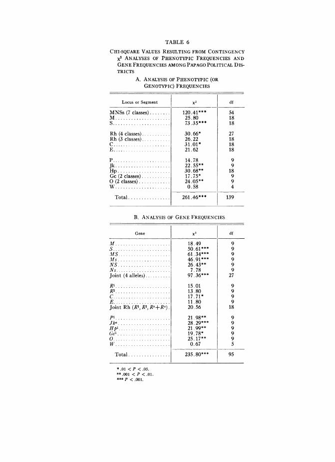
TABLE 6

CHI-SQUARE VALUES RESULTING FROM CONTINGENCYX2 ANALYSES OF PHENOTYPIC FREQUENCIES ANDGENE FREQUENCIES AMONG PAPAGO POLITICAL DIS-TRICTS

A. ANALYSIS OF PHENOTYPIC (ORGENOTYPIC) FREQUENCIES

Locus or Segment

MNSs (7 classes).M.....................S......................

Rh (4 classes)...........Rh (3 classes)...........C......................E ....

P......................Jk .....................Hp ....................Gc (2 classes)...........0 (2 classes)............w.....................

Total ................

x2

120.41***25.8073 .35***

30.66*26.2231.01*21.62

14.7822.55**30.68**17.75*24.05**0.58

261 .46***

df

541818

27181818

9918994

139

B. ANALYSIS OF GENE FREQUENCIES

Gene

M.....................

S......................MS ... .... ..... ....

Ms ....................NS ....................Ns ...................Joint (4 alleles)..........

R'......................R2 .. .. .. .. .. .. .. .. .. .. .

C......................E......................Joint Rh (RI, R2, RZ+RO).

.

Jka ....................Hp' ....................GO~...0......................w.....................

Total ................

x2

18.4950.61***61. 34***46.91***26. 43**7.78

97.36***

15.0113.8017. 71*11.8020.56

21. 98**28.29***21. 99**19. 78*25. 17**0.67

235.80***

df

999999

27

999918

999995

95

*.01 < F < .05.**.001 < P <.01.*** P < .001.

l~-


This provides additional support for the hypothesis that, with respect to the patternof genetic variation, the Papago districts are significantly different. However, dif-ferences in genotypic proportions among districts may result not only from dif-ferences in gene frequencies but also from variation in the mating system (e.g., in-breeding) or in the pattern of selection. Thus, although there are significant differ-ences among districts, we cannot specify the nature of the differences.

Interdistrict Heterogeneity of Gene FrequenciesIn order to determine whether the significant heterogeneity in the genotypic

distributions reflects differences in gene frequencies, the variation in genic propor-tions among districts was subjected to a contingency chi-square analysis. The for-mulas for computing the x2 statistics are of some interest. Suppose that we have rsamples of size Ni (i = 1, 2, . . ., r; 2Ni = N). If there are only two alleles at alocus, in frequencies pi and qi = (1 - pi), in each district, then the elements in theith row of the contingency table will be pi (2Ni) and qi (2Ni), since there are 2N genesin a sample of N individuals. Snedecor and Irwin (1933) proposed a short computa-tional formula for the contingency x2 value, which, for genic analyses, is given by

X2 = 2(2Ni)p2-p2(2Ni)pi (1)

pqwhere P and q denote the weighted means of the pi and qi (i.e., P = 2[Ni/N] pi).

If -2 denotes the weighted variance of the pi (c-2 = 2(Ni/N)p~ -p2), then thevalue of the x2 statistic given by (1) can be shown to be equal to

X2= pqP (2)

In general, if there are k alleles at a locus, then the x2 value for the correspondingr X k contingency table will be equal to

X2 =: 2N ( 'Ip(3,)j~~~~~~~~~3where pij and o-j denote the mean and variance of the frequencies of the jth allele.Thus, the genic contingency x2 is a function of the total sample size and the meansand variances of the gene frequencies. This result has a special significance in thegenetic analysis of population structure, as will be shown later.The results of the analysis are given in table 6. Several comparisons are significant

at the 5% level, and the frequencies of the MS, Ms and Jka alleles were significantlyheterogeneous at the 0.1% level. As before, x2's from independent comparisons(i.e., independent loci) were combined to provide an overall test of the heterogeneity.The total x2 is significant at the 0.1% level (table 6). These results show that thereare highly significant differences among the gene pools of the Papago districts andconfirm the anthropological observations suggesting considerable local genetic dif-ferentiation in the Papago.

The x2's for both genotypic and genic heterogeneity vary considerably both among

31

WORKMAN AND NISWANDER

alleles at a locus and among loci (table 6). When a proportion of the heterogeneityis due to random genetic drift, the observed heterogeneity at a locus (4.2) will varyabout some mean value (e2). Additional variation might be due to sampling. It isalso possible that variation in the amount of genetic differentiation, among allelesor loci, could result from biological phenomena. Suppose that there were a balanceof selective forces acting to maintain a given gene frequency. Then the frequenciesof that gene might show considerably less dispersion than the frequencies of anothergene on which the balance of selective forces was approximately neutral. Althoughthe cause of the variation in the x2 values cannot be determined by analysis of thepresent data, a comparison of the patterns of variation in different populations mightprovide some insight into the selective forces. If, for example, the x2 value associatedwith a specific locus were larger (or smaller) than the other x2 values significantlymore often than random sampling theory would predict, the existence (or absence)of selective forces could be inferred.

ANALYSES USING F STATISTICS

Theoretical ConsiderationsThe genetic structure of a subdivided population can also be analyzed by means

of Wright's F statistics. This is a heterogeneous group of statistics which provide amethod for partitioning an observed pattern of genetic variation or genetic relation-ships. They include inbreeding coefficients derived from pedigrees (or genealogies)which give the probability that two alleles at a locus in an individual are identicalby descent, correlations, functions of the amount of heterozygosity at a locus, andvariances and covariances of gene frequencies in subdivided populations. Each set ofF statistics used to describe a given observed population is derived with reference toa single specified foundation population, real or theoretical.

In the following discussion we shall be concerned only with those F statistics usedto analyze the genetic structure of a subdivided population. The mathematicaltheory for such an analysis is given by Wright (1943a, 1951, 1965) and Nei (1965).Here only the essential formulas and concepts will be mentioned.

The genotypic proportions at a single diallelic locus, say (A A, Aa, aa) = (P,H, Q), where P + H + Q = 1, can be represented in terms of the gene frequenciesof A and a, denoted by p and q, and a single F statistic, say F (called a fixationindex), by the formulas

AA Aa aaP=p2+pqF; H= 2pq(1-F); Q= q2+pqF, (4)

where p = P + WH, q = 1-p = Q + WH, and F = 1 - H/2pq. Here F denotesthe net deviation from Hardy-Weinberg proportions due to the joint effect of allforces acting on the pattern of genetic variation, including nonrandom mating,selection, and mutation. When inbreeding is the only factor, F is identical withthe classical inbreeding coefficient. The above formulation (4) provides a methodfor comparing different populations in terms of their net deviation from a singletheoretical model, that is, a population in which the genotypic proportions are asexpected under Hardy-Weinberg assumptions.

32

GENETIC DIFFERENTIATION IN THE PAPAGO 33

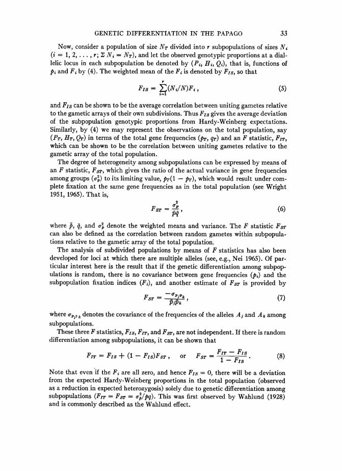
Now, consider a population of size XT divided into r subpopulations of sizes Ni(i = 1, 2, ... , r; Ni = X7), and let the observed genotypic proportions at a dial-lelic locus in each subpopulation be denoted by (Pi, Hi, Qi), that is, functions ofpi and Fj by (4). The weighted mean of the Fi is denoted by Fps, so that

Fis = Z(Ni/N)Fi, (5)i=i

and Fis can be shown to be the average correlation between uniting gametes relativeto the gametic arrays of their own subdivisions. Thus F1s gives the average deviationof the subpopulation genotypic proportions from Hardy-Weinberg expectations.Similarly, by (4) we may represent the observations on the total population, say(PT, HT, QT) in terms of the total gene frequencies (PT, qT) and an F statistic, FIT,which can be shown to be the correlation between uniting gametes relative to thegametic array of the total population.

The degree of heterogeneity among subpopulations can be expressed by means ofan F statistic, FST, which gives the ratio of the actual variance in gene frequenciesamong groups (a2) to its limiting value, PT(l - PT), which would result under com-plete fixation at the same gene frequencies as in the total population (see Wright1951, 1965). That is,

2

FST = UP (6)

where p, q, and U2 denote the weighted means and variance. The F statistic FSTcan also be defined as the correlation between random gametes within subpopula-tions relative to the gametic array of the total population.The analysis of subdivided populations by means of F statistics has also been

developed for loci at which there are multiple alleles (see, e.g., Nei 1965). Of par-ticular interest here is the result that if the genetic differentiation among subpop-ulations is random, there is no covariance between gene frequencies (pi) and thesubpopulation fixation indices (Fi), and another estimate of FST is provided by

FST = ' k (7)PjPk

where oPj, .denotes the covariance of the frequencies of the alleles A j and Ak amongsubpopulations.

These three F statistics, Frs, FI, and FST, are not independent. If there is randomdifferentiation among subpopulations, it can be shown that

FIT= FIs + (1-FIs)FST, or FST = 1-T FIS (8)

Note that even if the Fi are all zero, and hence FIs = 0, there will be a deviationfrom the expected Hardy-Weinberg proportions in the total population (observedas a reduction in expected heterozygosis) solely due to genetic differentiation amongsubpopulations (FI = FST = - ?pq). This was first observed by Wahlund (1928)and is commonly described as the Wahlund effect.

33

34 WVORKMAN AND NISWANDER

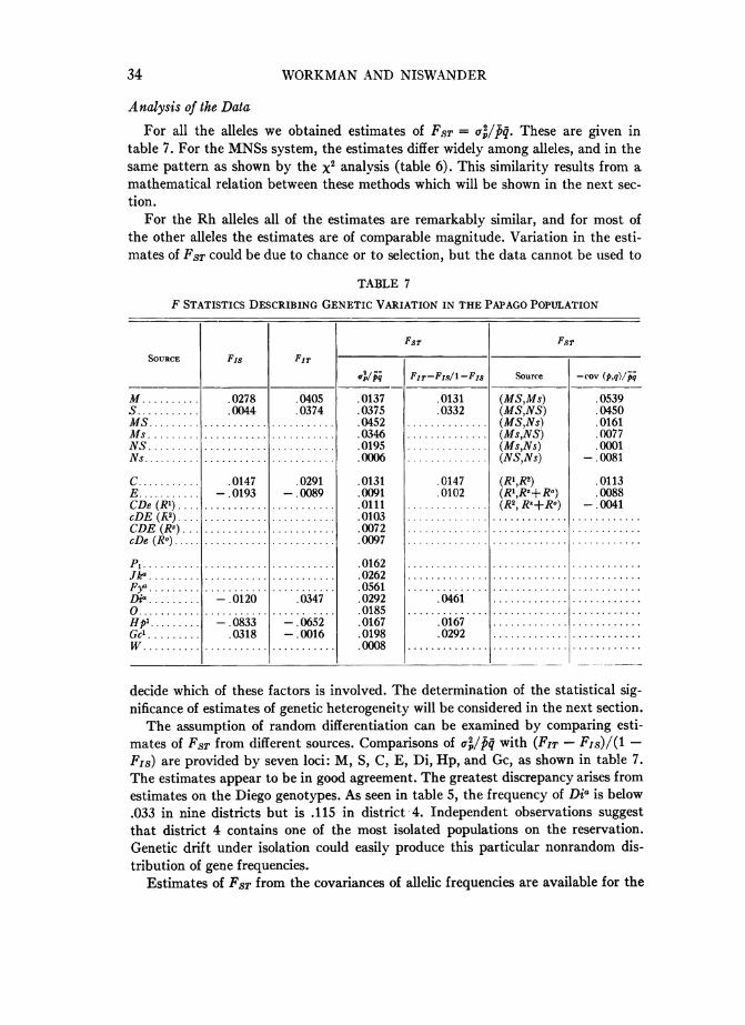
Analysis of the Data

For all the alleles we obtained estimates of FST =oT pq. These are given intable 7. For the MNSs system, the estimates differ widely among alleles, and in thesame pattern as shown by the x2 analysis (table 6). This similarity results from a,mathematical relation between these methods which will be shown in the next sec-tion.

For the Rh alleles all of the estimates are remarkably similar, and for most ofthe other alleles the estimates are of comparable magnitude. Variation in the esti-mates of FST could be due to chance or to selection, but the data cannot be used to

TABLE 7

F STATISTICS DESCRIBING GENETIC VARIATION IN THE PAPAGO POPULATION

FSTFSSoURCE Fjs F,

q F,T -Fjs/ I- Fis Source -(Ov (p,q)' pq

1 ......... .0278 .0405 .0137 .0131 (.M1S,AMs) .0539S ........ .0044 .0374 .0375 .0332 (MS,NS) .0450MS ... ......... ............ 0452.(.. SN .0161rs ....... .0346 .............. (Jls,NS) .0077

NS ....... .0195 ...N......... ( 11sNs) .0001Ns..0006 . ......I(NSNs) . 0081s .00 6 s - .00

C ........ .0147 .0291 .0131 .0147 (R1,R') .0113E........ -. 0193 -.0089 .0091 .0102 (R1,R+±R') .0088CDe (R1). .............. .0111 (RI, RZ+Ro) -.0041cDE (KX). ............. .0103CDE (Rz) ... ....... .......... .0072

....R0) ........ .. ... . ... .... ......0097.1.... .... .... ......cDe (RI, 0097

pi .0162......

Jk........... .0262F ......... ........... ........... .0561.... ........1 ..... ... .. ...

Di(t .... -. 0120 .0347 .0292 .0461 ............

.0185 ........ .. ....Hp'.......... .0833 - .0652 .0167 .0167 ...........

(;61 .....0..0318 - .0016 .0198 .0292 ........

1.. .0008 .....

decide which of these factors is involved. The determination of the statistical sig-nificance of estimates of genetic heterogeneity will be considered in the next section.

The assumption of random differentiation can be examined by comparing esti-mates of Fs8 from different sources. Comparisons of U21pq with (FIT - Fis)l(1-F1s) are provided by seven loci: M, S, C, E, Di, Hp, and Gc, as shown in table 7.The estimates appear to be in good agreement. The greatest discrepancy arises fromestimates on the Diego genotypes. As seen in table 5, the frequency of Dia is below.033 in nine districts but is .115 in district 4. Independent observations suggestthat district 4 contains one of the most isolated populations on the reservation.Genetic drift under isolation could easily produce this particular nonrandom dis-tribution of gene frequencies.

Estimates of FST from the covariances of allelic frequencies are available for the


MNSs and Rh systems (table 7). The MNSs estimates vary considerably but forthe Rh system the estimates all agree well with those from other sources. The meanvalue of FST estimated by o/p8, in table 7 (12 entries using M, S, C, E), is .0256;and the mean value estimated by (FIT- F1s)/(1 - FIs) is .0233. Although theseestimates are in quite good agreement, the fit with the estimate from the covariances(at only two loci) is less satisfactory.

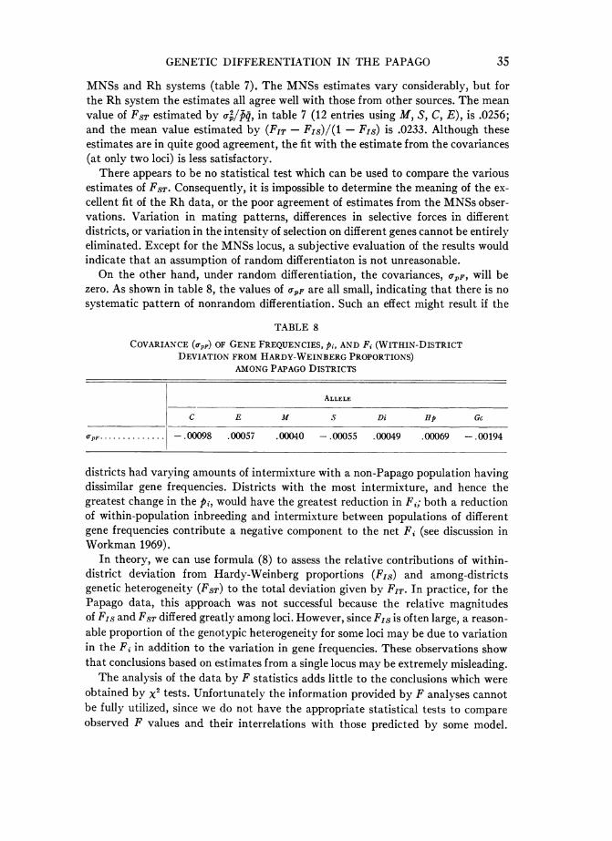
There appears to be no statistical test which can be used to compare the variousestimates of FST. Consequently, it is impossible to determine the meaning of the ex-cellent fit of the Rh data, or the poor agreement of estimates from the MNSs obser-vations. Variation in mating patterns, differences in selective forces in differentdistricts, or variation in the intensity of selection on different genes cannot be entirelyeliminated. Except for the MNSs locus, a subjective evaluation of the results wouldindicate that an assumption of random differentiaton is not unreasonable.On the other hand, under random differentiation, the covariances, JpF, will be

zero. As shown in table 8, the values of apF are all small, indicating that there is nosystematic pattern of nonrandom differentiation. Such an effect might result if the

TABLE 8

COVARIANCE (6pF) O GENE FREQUENCIES, pi, AND Fi (WITHIN DISTRICTDEVIATION FROM HARDY-WEINBERG PROPORTIONS)

AMONG PAPAGO DISTRICTS

ALLELE

C I M S Di lIp Gc

.....- 00098 .00057 .00040 -.00055 .00049 .00069 -.00194

districts had varying amounts of intermixture with a non-Papago population havingdissimilar gene frequencies. Districts with the most intermixture, and hence thegreatest change in the pi, would have the greatest reduction in F1; both a reductionof within-population inbreeding and intermixture between populations of differentgene frequencies contribute a negative component to the net Fi (see discussion inWorkman 1969).

In theory we can use formula (8) to assess the relative contributions of within-district deviation from Hardy-Weinberg proportions (FIs) and among-districtsgenetic heterogeneity (FST) to the total deviation given by FIT. In practice, for thePapago data, this approach was not successful because the relative magnitudesof FIs and FST differed greatly among loci. However, since FIS is often large, a reason-able proportion of the genotvpic heterogeneity for some loci may, be due to variationin the Fi in addition to the variation in gene frequencies. These observations showthat conclusions based on estimates from a single locus may' be extremely misleading.The analysis of the data by F statistics adds little to the conclusions which were

obtained by x2 tests. Unfortunately the information provided by F analyses cannotbe fully utilized, since we do not have the appropriate statistical tests to compareobserved F values and their interrelations with those predicted by some model.

35


Since the F statistics describe features of population structure which do not appearsusceptible to x2 analysis, the development of such tests would be of great use. Com-parisons of the values of FIT in different populations might provide evidence for theexistence of selective forces. For example, if at locus A there were greater net hetero-zygote advantage than at locus B, we should observe FIT(A) < FIT(.B) significantlymore often than would occur by chance. Comparisons of this kind are now in progressand will be reported elsewhere.

CHI-SQUARE AND F STATISTICS

We have thus far analyzed genetic variation in the Papago using two methods:x2 statistics and F statistics. A brief discussion of the mathematical relationshipsbetween these approaches should provide a greater understanding both of the methodsand of the conclusions drawn from such analyses.

Comparisons with Hardy-Weinberg Expectations

The comparison of observed genotypic proportions (P, H, Q) in a population ofsize N is, by the arguments already presented, a test to determine the probabilitythat a sample is drawn from a population in which the actual value of F (say 4) isequal to zero. As shown by Li and Horvitz (1953), the x2 statistic comparing observedand expected genotypic proportions is given by

X2 = F2N,1(9)where N is the sample size and F is estimated by F = 1 - H/2pq. That is, F2 =x2/N, which, for a 2 X 2 contingency table, is called the mean square coefficient ofcontingency. Further, F = (X2/N)112, for a 2 X 2 table, is also the coefficient ofcontingency described by both Tschuprow and Cramer as the most useful measureof association in a contingency table. In general, Cramer's coefficient of contingencyis defined by C = {x2/N min (r - 1, c -1)} 1/2, where r and c denote the numberof rows and columns in the contingency table (see discussion in Kendall and Stuart1961).Workman (1969) discussed a number of reasons why F will be close to zero, on

the average, not only in large random-mating populations but also in small popula-tions in which there are both inbreeding and differential fertility. Selection may eitherincrease, decrease, or leave unchanged the value of F. Inbreeding, positive assortativemating, and subdivision increase F, but avoidance of consanguinity, differentialfertility, and intermixture reduce F. From (9) it is clear that if F is near zero, thenF2N will also, in general, be small, and tests of deviation from Hardy-Weinbergproportions will rarely be significant.

Analysis of Gene Frequency Variation

By (2), the x2 statistic describing heterogeneity in the genic contingency-tableanalvsis, say x3, is geven by X2 = (2NT) o-/lpq. Also, by (6), FST = 4P/#q, so that

FST = X2/2NT, or FST2NT = X2(

36

(10)


For a k-allelic locus, under random differentiation, the estimates of FST for each alleleshould be identical. Under these conditions it can be shown that the x2 for thej X kgenic contingency table is given by x2 = 2NT (k - 1)FsS.

Thus, FST is a simple function of the x2 statistic, and, clearly, the significance ofan estimate of FST depends directly upon the significance of the x2 statistic. Thebest single estimate of genetic heterogeneity in a population is given by z X2, wherethe summation is over all independent loci.

Further, it is obvious that neither a single FST nor an average FST over loci is use-ful for interpopulation comparisons of heterogeneity when sample sizes vary. Aswill be demonstrated later, such comparisons can be made by an F-ratio test of thevalues of z x2 from each population.We may also write (10) as A\FST = (X2/2NT)"2" which is Cramer's coefficient of

contingency, C, for a j X 2 contingency table. It is of interest to note that Wright(1943a) suggested that the best measure of heterogeneity in a subdivided populationis given by V/42/pq = VFST. Both x2 and F values describe observed deviation fromtheoretical expectations, and the relation getween F and C, in at least two cases,provides a mathematical demonstration of the logical equivalence of these tech-niques.

Genotypic A nalysis

Unfortunately, we have not found a simple relation between the genotypic(phenotypic) contingency x2, say x4, and the F statistics. It can be shown, however,that x4 is of the form x4 = A a' + B o p+ C apF, where A, B, and C are functionsof pi, F., and FIT. Thus there is a direct relation between the x2 statistic and the Fstatistics. Note, even when Up = UpF = 0, there can be genotvpic heterogeneity dueto variation among the Fi. Under random differentiation, UpF = 0, and it may bepossible to derive a simple formula for the genotvpic contingency x2, say xp, basedon such an assumption. A statistical test of random differentiation would be providedby a comparison of the observed and expected x2's.

The Estimation of Sampling Error

The determination of the proportion of genetic variation due to sampling error is arather complex problem. In small populations, especially for gene frequencies de-termined by gene counting, if a large proportion of the population is examined, thereis really very little "sampling error"; and in such situations we may choose to ignoresampling effects entirely. On the other hand, if the sample contains only a smallproportion of the population, sampling error may provide a substantial part of theobserved genetic variation. Since conclusions in the present analysis do not dependupon the significance of the estimates of FIS, FI7, and X4, no corrections for samplingerror in these estimates were obtained. However, the contribution of sampling errorsto the estimates of genetic heterogeneity (FST or x = 2i\T FST) are of particularinterest. If the sample sizes are all large, the amount of sampling error may approxi-mate that given by a theoretical model of sampling from an infinite population. Forthe case of codominant alleles, the correction for sampling error in the estimates ofFST and x4tunder such conditions is given below.

37


The value of XG is inflated by an amount due to sampling error in the estimate ofap, which is approximately P (1- P)/2NT if sample sizes are proportional to the totalnumbers in each group. The corrected x2, say xG', is

2 ~7T2 P( - -)XG' = aNTtp 2NT / (11)

2NTTa 2

-. lP) 1 = 2NATFST'where FST' is the estimate of heterogeneity corrected from sampling error. That is,FST' is equal to FST -1/2NT, or, for the Papago population, FST'- FST - .0008.Similarly, for a diallelic comparison, XG2 = X- 1. It is obvious that the values ofXG in table 6 are sufficiently large that such a correction would not affect the sig-nificance of the results. We may conclude that sampling error of this type has nothad any effect.

Note that the correction here is only for sampling error resulting from drawing asample of size NT from the total population. The corrected cr, and hence FST',and XG', will include both the effects of real differences in gene frequencies amongdistricts and also variation solely due to subdivision of the sample into r groups.Therefore, according to this model of F statistics, FST will be nonzero even if thereare no genetic differences among subpopulations.

It is of interest to determine the values of FST and xG which would be obtainedby drawing r random samples from a single homogeneous population. If the Ni areequal, then NT = rNi, and the expected variation among the random samples isgiven by r2 =2 (1 -P)/2Ni, or a/P (1 -P) = 1/2Ni. Substituting into (11),we have X2' = (2NT/2Ni) - 1 = r - 1. This is the well-known result that for acomparison of random samples the expected value of a x2 statistic is equal to itsdegrees of freedom. Also, the corrected value of FST under these conditions is givenby FST' = 1/2Ni- 1/2NT (see [12]). In general, for a joint r X k comparison of thefrequencies of k alleles it can be shown that x' = (k - 1) (2NTFST - 1) = XG-(k - 1). Under random sampling effects, the expected values of XG and XG' are (k -1) r and (k - 1) (r - 1), respectively.

Since the significance of FST depends directly upon the significance of XG, whichtakes into account the effects of subdivision, there is no need to subtract from 42 acomponent due to random sampling among subdivisions (approximately Pq/2Ni) inorder to make the expected value of FST equal to zero. This latter approach wasused by Nei and Imaizumi (1966a, 1966b, 1966c), in their studies on local differentia-tion in Japanese populations. They provided an approximate test to determine thesignificance of an estimate of FST with an expected value close to zero (but not exactlyzero, since there was no correction for sampling of the total population, a =p2NT).

In most studies, estimates of genetic variation (4') will also include the effectsof dominance and of sampling from a finite population. Formulas providing exact

corrections are not available, but Wright (1943b) provided approximations for thecase of equal subpopulation sizes, and Nei and Imaizumi (1966a) give formulas which

38


can be used when subpopulation size varies. When Wright's formulas were applied tothe Papago data, the values of FST and x< were reduced, but significant differentiationamong districts was still evident. Since these formulas depend on sample size per sebut do not reflect the actual proportions of the total population sampled, their ap-plicability in this study is questionable. Finally, it should be noted that normalapproximations used to test the significance of a x2 statistic with v > 30 are based onthe distribution of the corrected x2's. However, for large v, they may also be used totest the significance of an uncorrected x2, as was done earlier in this paper.

THE CAUSES OF HETEROGENEITY

The analysis in the previous sections has demonstrated significant genetic dif-ferentiation among Papago districts, essentially by comparing the actual pattern ofvariation with that which would result from random sampling effects alone. Suchan analysis, however, provides no information about the various factors responsiblefor the genetic heterogeneity. In this section, utilizing additional sources of informa-tion about the Papago population, we shall attempt to identify those factors pri-marily responsible for the observed variation.

First, there may be differentiation due to a "founder effect." That is, there mayhave been genetic differences among the ancestral populations which gave rise tothe individuals in the present Papago districts. Although there is evidence whichsupports a hypothesis of initial heterogeneity, it is rather imprecise. Historical studiesshow that different Indian groups have contributed to the present Papago populationand that each group probably had most of its effect in a specific geographic region(see Niswander et al. 1970). For example, the Indians in district 9 may be more

closely related to the Pima Indians living to the north of the Papago reservationthan to other Papagos. Those in the western part of the reservation, especially indistricts 4 and 5, are said to be descendants of related ancestral groups, and the south-ern districts contain numerous descendants of migrants from Mexico. The dialect dif-ferences within the Papago population may have arisen recently, but there is evi-dence that they reflect heterogeneity in the ancestral population. Finally, the in-habitants of districts 7, 8 (especially the town of Sells), and 10 (San Xavier) are notdescendants of original populations in those areas but of Papagos who have movedto these locations during the past 75 years.

Although there probably was genetic diversity among the ancestral populations,the extent to which the current genetic heterogeneity results from differences in thefounder populations cannot be determined. However, since interpopulation compari-sons among Indian tribes in the southwest do not reveal any large genetic differences(Brown et al 1958; Niswander et al. 1970), there may have been cultural differencesamong the founders of the Papago unaccompanied by significant genetic variation.The relation between genetic differentiation and isolation by distance has been

studied in a number of human populations. If the movement of individuals is general-ly restricted to an area less than that occupied by the total population, then the proba-bility that two individuals will marry is based not on random expectations but ratheron the geographic distance separating them. That is, there will be a decrease in thefrequency of marriages as the distance between mates increases. Thus, in such

39


populations there will be local genetic differentiation. As the distance between in-dividuals (or groups) decreases, their degree of relationship and, hence, the similarityin their pattern of genetic variation will increase.

In large populations in which the distances between individuals or groups areapproximately continuously distributed, isolation by distance is revealed by demon-strating that the coefficient of kinship between random pairs of individuals or groupsdeclines as the distance between them increases (e.g., Malecot 1966; Morton et al.1968). In effect, the covariance of gene frequencies among all groups at a distance,say d, decreases as d increases.

Isolation by distance can also be considered in a population subdivided intoa small number of geographically distinct subpopulations by comparing the geneticdistance between pairs of subpopulations with the geographic distances separatingthem. The genetic distance between groups is defined following a suggestion bySanghvi (1953). For each pair of subpopulations and for each independent k-alleliclocus, differences in the gene frequencies can be compared by means of a 2 X kcontingency x2 with (k - 1) degrees of freedom. Since independent x2's can be com-bined for a total of n independent loci, we can then define an overall genetic distanceG for each pair of subpopulations, by

G k1: (pij - qi)2 + (p'ij - q (12)i=1j=1 qij qij

where pij and p'j are the frequencies of thejth allele at the ith locus in the two groupsand qij = (pij + p'j)/2. For ease of computation the above may also be written as

G= . E hp, - pi)2 (13)

It is obvious that for two groups with identical gene frequencies, G will be zero andG will increase as the genetic differences between the groups increase.

If different loci are used for different pairs of subpopulations, genetic distancescan be compared by considering G' = G/2 df where 2 df denotes the total degrees offreedom for the x2's involved in the summation. Since the estimate of G does not takeinto account variation in sample size but depends only on gene frequency estimates,sample sizes should represent equivalent proportions of the total population in eachgroup.

Geographic distances may be measured in different ways. Since straight-line mapdistances between populations ignore geographic barriers to population movement,we have defined geographic distance for the Papago as the shortest distance by roador trail (used by the Indians) between the centers of population in each district. Inmost districts the center of population is simply the single large village in that dis-trict. For districts with two or more large villages, the center was assumed to liebetween the villages at distances proportional to the village population sizes.

The values of G and the geographic distances (expressed in miles) for each pair ofPapago districts are provided in table 9. The values of G are based on an overallcomparison among the following loci: Rh (R1, R2, RK + RK), MNSs (MS, Ms, NS, Ns),

40

GENETIC DIFFERENTIATION IN THE PAPAGO 41

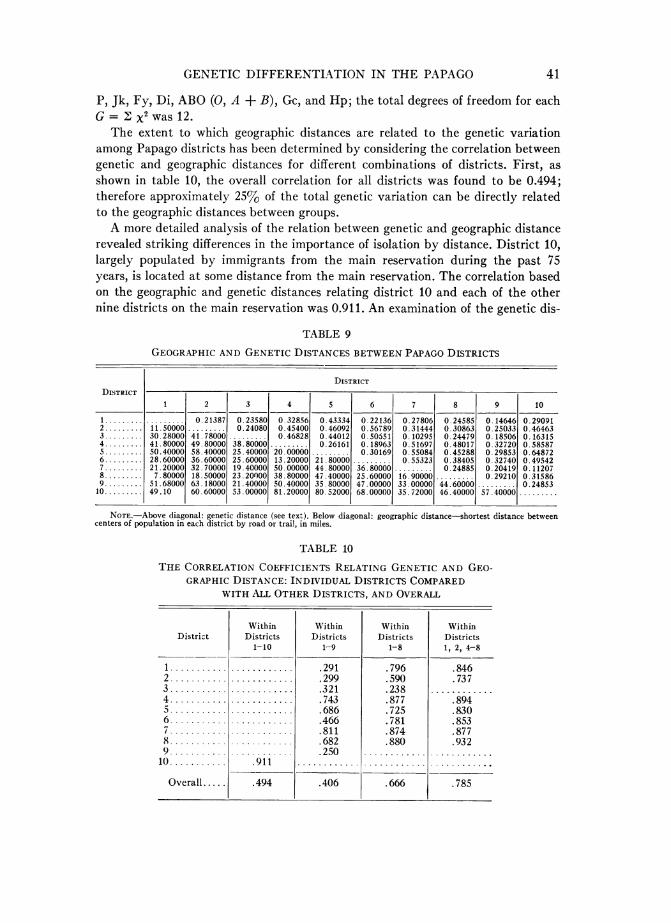
P. Jk, Fy, Di, ABO (0, A + B), Gc, and Hp; the total degrees of freedom for eachG = z %2 was 12.

The extent to which geographic distances are related to the genetic variationamong Papago districts has been determined by considering the correlation betweengenetic and geographic distances for different combinations of districts. First, asshown in table 10, the overall correlation for all districts was found to be 0.494;therefore approximately 25% of the total genetic variation can be directly relatedto the geographic distances between groups.A more detailed analysis of the relation between genetic and geographic distance

revealed striking differences in the importance of isolation by distance. District 10,largely populated by immigrants from the main reservation during the past 75years, is located at some distance from the main reservation. The correlation basedon the geographic and genetic distances relating district 10 and each of the othernine districts on the main reservation was 0.911. An examination of the genetic dis-

TABLE 9

GEOGRAPHIC AND GENETIC DISTANCES BETWEEN PAPAGO DISTRICTS

DISTRICTDISTRICT

1 2 3 4 5 6 7 8 9 10

1...... ......... 0.21387 0.23580 0. 32856 0.43334 0.22136 0.27806 0.24585 0. 14646 0.290912....... 1150000 0.24080 0 .45400 0 .46092 0.56789 0.31444 0.30863 0 .25033 0.464633....... 30 28000 41 .78000 0.46828 0.44012 0. 5051 0.10295 0.24479 0. 18506 0.163154....... 41.80000 49. 80000 38.80000.. 0.26161 0. 18963 0.51697 0.48017 0. 32720 0. 585875....... 50.40000 58 .40000 25.40000 20.00000. 0 30169 0 .55084 0.45288 0.29853 0.648726....... 28.60000 36.60000 25.60000 13.20000 21 .80000 ... 0.55323 0.38405 0. 32740 0.495427....... 21.20000 32.70000 19.40000 50 .00000 44.80000 36.80000. 0. 24885 0.20419 0.112078....... 7. 80000 18.50000 23.20000 38. 80000 47. 40000 25.60000 16 90000 0.29210 0.315869....... 51.68000 63.18000 21.40000 50.40000 35.80000 47.00000 33.00000 44.60000. 0.2485310 ....... 49.10 60. 60000 53.00000 81.20000 80. 52000 68. 00000 35.72000 46.40000 57.400000..

NOTE.-Above diagonal: genetic distance (see text). Below diagonal: geographic distance-shortest distance betweencenters of population in each district by road or trail, in miles.

TABLE 10

THE CORRELATION COEFFICIENTS RELATING GENETIC AND GEO-GRAPHIC DISTANCE: INDIVIDUAL DISTRICTS COMPARED

WITH ALL OTHER DISTRICTS, AND OVERALL

Within Within Within WithinDistrict Districts Districts Districts Districts

1-10 1-9 1-8 1, 2, 4-8

1. ........... .291 .796 .8462........... ... .299 .590 .7373.... . .321 .238 ............

4........... .743 .877 .8945... .686 .725 .8306.... ... .... .466 .781 .8537/.. .. ... .. .811 .874 .8778.. ... .... .682 .880 .9329. ... .. .250 ... .. ..........

10 ....... .911 ............ ............

Overall..... .494 .406 .666 .785


tances between district 10 and the other groups agrees with the historical evidencesuggesting primary colonization from districts 3 and 7. The overall correlation showsan almost perfect inverse relation between an individual's distance from district 10and his likelihood of moving there.

Within the Sells reservation there is also variation in the pattern of correlationsrelating each district to the other eight districts (table 10). The lowest correlation isthat between district 9 and the others (r = 0.250). As mentioned previously, thepopulation in district 9 originated from a separate group, the Kohatk, who have had atraditional close association with the Pima Indians. Thus, there may have beenvery little contact between district 9 and most of the remainder of the reservation.

Excluding district 9, the overall correlation on the reservation is 0.666, so that 44%0of the genetic variation among these districts is related to the geographical distancesbetween them. Only district 3 shows a low correlation (r = 0.238) with the others.The genetic distance between districts 3 and 7 is very close, as would be predictedby the historical evidence that district 7 was populated primarily by immigrants fromdistrict 3. The genetic distances between district 3 and districts 1, 2, 8, and 9 areof the same magnitude (0.185-0.245); the distances between district 3 and districts4, 5, and 6 are similarly close (0.440-0.507). District 3 is known to have had continualand extensive interaction with district 9 and has also had association with the Pima(Mark 1960). A relationship between districts 3 and 9 is seen in table 9; the geneticdistance between them is among the smallest for any pair of districts. Thus the lowcorrelation between districts 9 and 3 with each of the other districts may be due totheir interaction with each other and with the Pima.When district 3 is eliminated from consideration, the overall correlation (among

districts 1, 2, and 4-8) rises to 0.785. The greatest correlation is between district 8and the others (r = 0.932). District 8 is largely populated by recent immigrants fromother parts of the reservation, probably because of greater opportunities for employ-ment with the recently established Indian Agency. As with San Xavier (district 10),it appears that the likelihood of moving to Sells is inversely related to the distanceinvolved. Even when districts 3 and 9 are included, the correlation of district 8 withothers on the reservation is 0.682.The results and observations thus far presented provide a basis for determining

which factors are responsible for the genetic heterogeneity among Papago groups.First, it seems likely that some variation results from differences among the ancestralpopulations in each area. It is also likely that the genetic differentiation has increaseddue to random genetic drift, since the districts contain small populations (300-1,000individuals) which have been highly endogamous for 250-300 years.A considerable proportion of the variation (25%-50%) can be ascribed to the

geographic distances between groups. Three indistinguishable factors may be re-

sponsible for the observed correlations. First, geographic distances may reflectoriginal differences (or similarities) in the pattern of variation. That is, adjacentdistricts may have been founded by closely related groups. Second, there may beisolation by distance in terms of an inverse relation between the frequency of in-terdistrict mating and geographic distance. Finally, the probability of migration tocertain districts appears to be inversely proportional to the distance involved. Thus,

42


over 75% of the heterogeneity resulting from comparisons of district 7, 8, and 10with the remainder of the reservation can be attributed to the relation betweendistance and migration.

The analysis of population structure is essentially a comparison among differenttypes of distance measures: biological, based on qualitative or quantitative traits;geographical, such as road distances or altitudinal differences; and, cultural, based onculture traits, linguistic patterns, etc. (see discussion in Howells 1966). In anyparticular study of intra- or interpopulation variation, some distance measures maynot be relevant, and there may not be sufficient information on others to deriveanalytical measures. In the present study only two specific distance measures wereutilized: (1) genetic distance based on nine qualitative traits and (2) a geographicdistance describing the minimum road or trail distance between centers of popula-tion in each district. However, the interpretation of the observations required addi-tional information on the historical relations among groups, mating patterns, lin-guistic differences, etc.We did not attempt to derive a distance measure for the Papago based on anthro-

pometric measurements. Such traits may be much less susceptible to forces such asgenetic drift, and results similar to those based on qualitative traits would probablyrequire both large samples and a large number of traits. On the Japanese islandKuroshima, for example, there was significant heterogeneity of the ABO frequenciesamong districts, but no significant differences among groups with respect to heightsand weights were observed (Schull et al. 1962). Unless there is some reason to expectvariation in physical measurements (e.g., ecological variation or differences in ethnicorigins), the effort required to obtain anthropometric data would probably be moreusefully employed in increasing the number of qualitative traits under study.

COMPARISONS WITH OTHER POPULATIONS

The foregoing analysis has established that the Papago population shows consider-able local differentiation of gene frequencies. In order to assess the significance of theresults, especially with regard to developing general theories of population structure,we shall compare the Papago with other populations of comparable size and geo-graphic distribution. In particular, we are interested in the extent to which localdifferentiation occurs, the amount of heterogeneity in different populations, and thecausal mechanisms involved.We can compare the variation in the real Papago population with that which

would be present if the 10 districts were 10 random samples drawn from a homo-geneous population. For this purpose, an artifically subdivided Papago populationwas created by assigning each individual to one of 10 subpopulations on the basis of atable of random numbers from 0 to 9. Subpopulation sizes were randomly distrib-uted about a mean of 68.1. The values of FST = c4/Mq and XG = 2NT FST for thisartificial population are given in table 11.By an analysis of the x2 values we can determine the extent to which the variation

in this artificial population corresponds to that predicted by the mathematical theory.In a previous section it was shown that for a population comprising r random samplesof size Ns, the expected value of the genic contingency x2 is equal to r if there is

43

44 WORKMAN AND NISWANDER

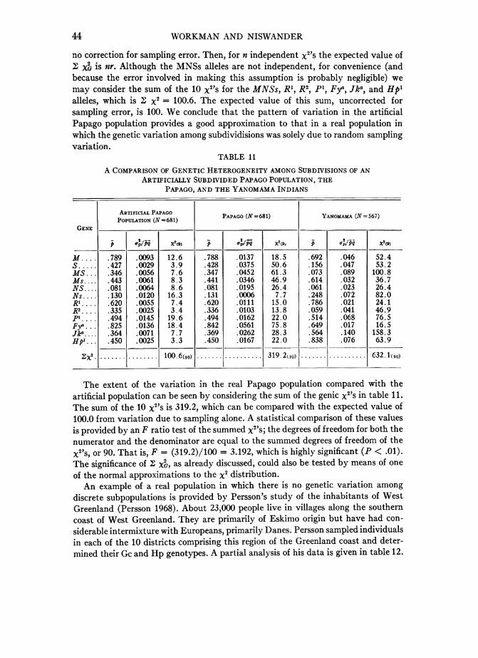
no correction for sampling error. Then, for n independent x2's the expected value ofz X' is nr. Although the MNSs alleles are not independent, for convenience (andbecause the error involved in making this assumption is probably negligible) wemay consider the sum of the 10 x2's for the MNSs, RI, R2, PI, Fya, Jka, and Hp'alleles, which is z x2= 100.6. The expected value of this sum, uncorrected forsampling error, is 100. We conclude that the pattern of variation in the artificialPapago population provides a good approximation to that in a real population inwhich the genetic variation among subdividisions was solely due to random samplingvariation.

TABLE 11

A COMPARISON OF GENETIC HETEROGENEITY AMONG SUBDIVISIONS OF ANARTIFICIALLY SUBDIVIDED PAPAGO POPULATION, THE

PAPAGO, AND THE YANOMAMA INDIANS

ARTIFICIAL PAPAGOPAPAGO (N=681) YANOMAMA (N 567)POPULATION (N =681)

GENE

___ \ up/Pq X2(9) P /pq/ X29, p /pq x (9)

M ... .789 .0093 12.6 .788 .0137 18.5 .692 .046 52.4S.... .427 .0029 3.9 .428 .0375 50.6 .156 .047 53.2MS. .346 .0056 7.6 .347 .0452 61.3 .073 .089 100.8Ms... .443 .0061 8.3 .441 .0346 46.9 .614 .032 36.7NS... .081 .0064 8.6 .081 .0195 26.4 .061 .023 26.4Ns .130 .0120 16.3 .131 .0006 7.7 .248 .072 82.0RI. .620 .0055 7.4 .620 .0111 15.0 .786 .021 24.1R .335 .0025 3.4 .336 .0103 13.8 .059 .041 46.9P1 . 494 .0145 19.6 .494 .0162 22.0 .514 .068 76.5Fy'. .825 .0136 18.4 .842 .0561 75.8 .649 .017 16.5Jk-a... .364 .0071 7.7 .369 .0262 28.3 .564 .140 158.3Hp'. .450 .0025 3.3 .450 .0167 22.0 .838 .076 63.9

2X2. ....... 100.6(90) ................. 319 2(90).......(.......... 632 1@O)

The extent of the variation in the real Papago population compared with theartificial population can be seen by considering the sum of the genic x2's in table 11.The sum of the 10 x2's is 319.2, which can be compared with the expected value of100.0 from variation due to sampling alone. A statistical comparison of these valuesis provided by an F ratio test of the summed x2's; the degrees of freedom for both thenumerator and the denominator are equal to the summed degrees of freedom of thex2's, or 90. That is, F = (319.2)/100 = 3.192, which is highly significant (P < .01).The significance of z XG, as already discussed, could also be tested by means of one

of the normal approximations to the x2 distribution.An example of a real population in which there is no genetic variation among

discrete subpopulations is provided by Persson's study of the inhabitants of WestGreenland (Persson 1968). About 23,000 people live in villages along the southerncoast of West Greenland. They are primarily of Eskimo origin but have had con-

siderable intermixture with Europeans, primarily Danes. Persson sampled individualsin each of the 10 districts comprising this region of the Greenland coast and deter-mined their Gc and Hp genotypes. A partial analysis of his data is given in table 12.

GENFETIC DIFFEIRENTIATION IN THE PAPAGO 45

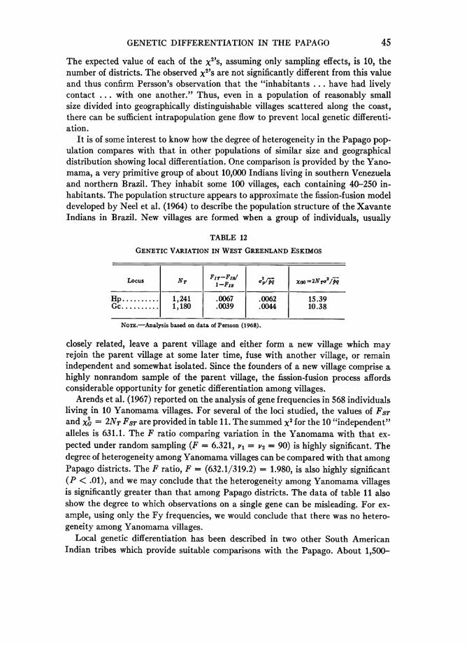
The expected value of each of the x2's, assuming only sampling effects, is 10, thenumber of districts. The observed x2's are not significantly different from this valueand thus confirm Persson's observation that the "inhabitants ... have had livelycontact ... with one another." Thus, even in a population of reasonably smallsize divided into geographically distinguishable villages scattered along the coast,there can be sufficient intrapopulation gene flow to prevent local genetic differenti-ation.

It is of some interest to know how the degree of heterogeneity in the Papago pop-ulation compares with that in other populations of similar size and geographicaldistribution showing local differentiation. One comparison is provided by the Yano-mama, a very primitive group of about 10,000 Indians living in southern Venezuelaand northern Brazil. They inhabit some 100 villages, each containing 40-250 in-habitants. The population structure appears to approximate the fission-fusion modeldeveloped by Neel et al. (1964) to describe the population structure of the XavanteIndians in Brazil. New villages are formed when a group of individuals, usually

TABLE 12

GENETIC VARIATION IN WEST GREENLAND ESKIMOS

Locus NT I_FIST / 2p/pq X(9) =2NTo/pq

Hp.1,241 .0067 .0062 15.39Gc .1,180 .0039 .0044 10.38

NOTE.-Analysis based on data of Persson (1968).

closely related, leave a parent village and either form a new village which mayrejoin the parent village at some later time, fuse with another village, or remainindependent and somewhat isolated. Since the founders of a new village comprise ahighly nonrandom sample of the parent village, the fission-fusion process affordsconsiderable opportunity for genetic differentiation among villages.

Arends et al. (1967) reported on the analysis of gene frequencies in 568 individualsliving in 10 Yanomama villages. For several of the loci studied, the values of FS7and xG = 2i\T FST are provided in table 11. The summed x2 for the 10 "independent"alleles is 631.1. The F ratio comparing variation in the Yanomama with that ex-pected under random sampling (F = 6.321, Vp = V.= 90) is highly significant. Thedegree of heterogeneity among Yanonmama villages can be compared with that amongPapago districts. The F ratio, F = (632.1/319.2) = 1.980, is also highly significant(P < .01), and we may- conclude that the heterogeneity among Yanomama villagesis significantly greater than that among Papago districts. The data of table 11 alsoshow the degree to which observations on a single gene can be misleading. For ex-ample, using only the Fy frequencies, we would conclude that there was no hetero-geneity among Yanomanma villages.

Local genetic differentiation has been described in two other South AmericanIndian tribes which provide suitable comparisons with the Papago. About 1,500-

45


2,000 Xavante Indians are distributed among at least seven villages in the Brazilianstate of Mato Grosso. Genetic and demographic studies (e.g., Neel et al. 1964;Salzano et al. 1967; Neel and Salzano 1967) have described their population structureas a fission-fusion type so that genetic heterogeneity among villages may be assumedto result from a type of founder effect. An overall genic heterogeneity x2 based on

the frequencies of 13 alleles studied in two or three villages is found to be x2 =129.62 with 24 degrees of freedom (data from Salzano 1968), a result which is highlysignificant. An F ratio comparison with the Papago data of table 11 yields F =

2.463 (v1 = 90, V2 = 24), so the heterogeneity among Papago districts is significantlygreater than that among Xavante villages (.005 < P < .01).

The Caingang Indians, numbering 3,000-4,000, live in a series of villages in fourstates of southern Brazil. Demographic and genetic studies on seven villages in thestates of Rio Grande do Sul and Santa Catarina have been reported by Salzano(1961, 1968). The villages are highly endogamous, and migration among them ap-pears to be related, in some degree, to the distances between villages. The hetero-geneity in this population, as in the Papago, is probably due to several generationsof random genetic drift and isolation by distance. The summed x2 for 13 alleles(data from Salzano 1968) is 185.22 with df = 39, indicating highly significant geneticheterogeneity among villages. The Papago, however, are found to have significantlygreater heterogeneity: F = 1.723 (.01 < P < .05).

Salzano (1968) compared intrapopulation variation in the Caingang and Xavantetribes in terms of the range of gene frequencies among villages. The range of fre-quencies among Caingang villages generally exceeds that observed in the Xavante.However, as noted by Salzano, differences in sample sizes and in the number ofvillages studied in each tribe make interpretation of the range of frequencies extremelydifficult. An F ratio comparison of the summed x2's, F = 1.429 (vl = 39, V2 = 24)shows no significant difference in heterogeneity (P > .10).

Only a small number of studies on non-Indian populations showing local dif-ferentiation provide comparisons with the Papago. Roberts et al. (1965), using onlyABO frequencies, demonstrated significant heterogeneity among villages in fivegeographically isolated regions on the Greek island of Tinos (X2 = 29.68 with df = 8).Considerable endogamy was observed within regions as well as within villages ineach region, suggesting that both geographic and culture barriers have promotedvillage isolation. Random genetic drift, opposed by small amounts of migrationamong villages on the island and by immigration from the Greek mainland, wouldappear to be the chief cause of the local differentiation.

Nei and Imaizumi (1966c) analyze heterogeneity with respect to ABO genefrequencies in six small Japanese populations. In five of the six there was significantlocal differentiation among subpopulations. For example, on the island of Kuroshimaabout 2,300 people are distributed among eight administrative districts (originaldata of Schull et al. 1962). One of the eight districts is exclusively inhabited by Bud-dhists, one includes a majority of Buddhists and some Catholics, and the othersix include only Catholics. The Buddhists and Catholics came from different areas

of Japan over 300 years ago. Buddhists and Catholics do not appear to intermarry,and there is considerable within-district endogamy in all eight districts. The ABO

46


gene frequencies were studied in 508 individuals distributed among the eight districts.The overall genic x2 for ABO heterogeneity, 65.1 with df = 14 (data of Schull et al.1962), is highly significant, and the heterogeneity would appear to be due to a com-

bination of founder effect and random genetic drift.Despite the small number of studies reviewed, it seems reasonable to assert that

it is impossible to make generalizations about the amount or causes of local differ-entiation in such populations. Each is of limited total size (N < 25,000) and de-finable geographic range and has a population distributed among geographicallydistinct regions. Local differentiation may be absent or extreme, of recent origin or

the result of diverse forces operating for several hundred years. The causes of hetero-geneity may involve founder effect, isolation by distance, or random genetic drift;in any given population any one or a combination of these factors may be most im-portant. The relative amount of heterogeneity cannot be predicted even when thechief factors responsible can be specified.

It should be noted that in the values of2 xG from different populations, theeffects of dominance will vary with the loci considered, and the effects of samplingerror will vary with the size of the population and the numbers and sizes of the sub-populations. Thus a critical comparison of the amounts of heterogeneity in two pop-

ulations would require appropriately corrected values of XG. The comparison ofheterogeneity in the Papago and in the Yanomama, utilizing the same loci and basedon equal numbers of subpopulations of approximately the same size, would probablybe least affected by the use of corrected Xi's. It also seems most unlikely that suchcorrections would affect our general observation that subdivided populations showconsiderable variation in their amounts of genetic heterogeneity. Finally, since ccm-

parisons based on X2 would remove dominance effects but include contributionsfrom U2 and 0pF, the use of

z xG appears preferable.These studies also show that demonstration of significant intrapopulation hetero-

geneity indicates nothing about the real structure of a population, past or present.For example, under a fission-fusion system there will almost always be significantheterogeneity among villages. However, because of the constant migration of groups

over a period of 5-10 generations, the genetic structure approximates that in a ran-

dom-mating population (Neel and Salzano 1967). Under such conditions, the amountof genetic heterogeneity would be expected to fluctuate around some mean valuefrom one generation to the next. In other populations, heterogeneity might be in-creasing, decreasing, or constant, depending upon the forces operative at any giventime. In the Papago the development of roads, the use of mechanical means of trans-port, and the centralization of public health and Indian agency facilities should in-crease contact among individuals formerly isolated, and we may expect a steadydecrease in the amount of local differentiation.

In this paper we have been concerned with the analyses of local differentiationin small populations which can be described by a stepping-stone model. Bodmer and

Cavalli-Sforza (1968) have presented mathematical formulas which can also be ap-

plied to data on such populations. Given the initial gene frequencies, subpopulationsizes, and the pattern of migration among groups, their formulas describe the gene

frequencies expected to result from the joint effects of random genetic drift and isola-

47


tion by distance, in each successive generation. An attempt to apply their formulasusing data on migration provided by the Papago Population Register will be pre-sented in another paper.

SUMMARY

The Papago Indian population living on two reservations in southern Arizona isdistributed among 10 partially endogamous, geographically distinguishable regions.The analysis of the population structure of the Papago was accompanied by a generaldiscussion of the methods used to analyze subdivided populations.By the use of x2 tests and Wright's F statistics, it was found that there are highly

significant, essentially random genetic differences among Papago groups. The rela-tion between x2 and F statistics was considered. It was shown that Wright's measureof genetic heterogeneity, FST = 0_/Pq, is equal to 2NT X2, where NT is the totalsample size and X2 is the x2 value for the contingency-table analysis of gene-fre-quency differences among groups. It was suggested that the best single measure ofgenetic heterogeneity in a subdivided population is given by z X2, where the sum istaken over all independent genes.By comparing genetic distances between groups with geographic distances, it

was found that a large proportion of the total variation could be attributed to isola-tion bv distance affecting both the frequencies of intergroup matings and the patternof migration into regions newly settled by the Papago. Other factors contributing tothe genetic heterogeneity include differences among the ancestral populations ineach region and random genetic drift.

Approximate comparisons of the amount of heterogeneity in different subdividedpopulations are provided by an F ratio test comparing values of z XG from eachpopulation. Populations similar in size and structure to the Papago show consider-able differences both in the amount of heterogeneity and in the factors primarilyresponsible for the local differentiation.

REFERENCESARENDS, T.; BREWER, G; CHAGNON, N.; GALLUNGO, M. L.; GERSHOWITZ, H.; LAYRISSE, M.;

NEEL, J.; SHREFFLER, D.; TASHIAN, R.; and WEITKAMP, L. 1967. Intratribal geneticdifferentiation among the Yanomama Indians of southern Venezuela. Proc. Nat. Acad.Sci. (U.S.A.) 57:1252-1259.

BODMER, W. F., and CAVALLI-SFORZA, L. L. 1968. A migration matrix model for the studyof random genetic drift. Genetics 59:565-592.

BROWN, K. S.; HANNA, B. L.; DAHLBERG, A. A.; and STRANDSKOV, H. H. 1958. The dis-

tribution of blood group alleles among Indians of southwest North America. Amer. J.Hum. Genet. lo: 175-195.

HOWELLS, W. W. 1966. Population distances: biological, linguistic, geographical, and en-

vironmental. Current Anthrop. 7:531-540.JONES, R. D. 1969. An analysis of Papago communities 1900-1920. Ph.D. diss., University

of Arizona, Tucson.KENDALL, M. D., and STUART, A. 1961. The advanced theory of statistics. Vol. 2. Inference and

Relationship. Hafner, New York.KIMURA, M., and WEISS, G. H. 1964. The stepping-stone model of population structure and

the decrease of genetic correlation with distance. Genetics 49:461-576.

48


Li, C. C., and HORVITZ, D. G. 1953. Some methods of estimating the inbreeding coefficient.Amer. J. Hum. Genet. 5:107- 117.

MALECOT, G. 1966. Probabilites et Hgrgdite. Presses Univ. de France, Paris.MARK, A. K. 1960. Description of variables relating to ecological change in the history of

the Papago Indian population. M.A. thesis, University of Arizona, Tucson.MORTON, N. E.; MIKI, C.; and YEE, S. 1968. Bioassay of population structure under isola-

tion bv distance. Amer. J. Hum. Genet. 20:411-419.NEEL, J. V., and SALZANO, F. M. 1967. Further studies on the Xavante Indians. X. Some

hypothesis-generalizations resulting from these studies. Amer. J. Hum. Genet. 19:554-574.NEEL, J. V.; SALZANO, F. M.; JUNQUEIRA, P. C.; KEITER, F.; and MAYBURY-LEwIs, D. 1964.

Studies on the Xavante Indians of the Brazilian Mato Grosso. Amer. J. Hum. Genet.16:52-140.

NEI, M. 1965. Variation and covariation of gene frequencies on subdivided populations.Evolution 19:256-258.

NEI, M., and IMAIZUMI, Y. 1966a. Genetic structure of human populations. I. Local differ-entiation of blood group gene frequencies in Japan. Heredity 21:9-35.

NEI, M., and IMAIZUMI, Y. 1966b. Genetic structure of human populations. II. Differentia-tion of blood group gene frequencies among isolated populations. Heredity 21:183-190.

NET, M., and IMAIzUMI, Y. 1966c. Genetic structure of human populations. III. Differentia-tion of ABO blood group gene frequencies in small areas of Japan. Heredity 21:461-472.

NLSWANDER, J. D.; BROWN, K. S.; IBA, B. Y.; LEYSHON, W. C.; and WORKMAN, P. L. 1970.Population studies on Southwestern Indian Tribes. I. History, culture, and genetics ofthe Papago. Amer. J. Hum. Genet. 22:7-23.

PERSSON, I. 1968. The distribution of serum types in West Greenland Eskimos. Acda Genet.Statist. Med. (Basel) 18:261-270.

ROBERTS, D. F.; LUTTRELL, Y.; and SLATER, C. P. 1965. Genetics and geography in Tinos.Eugen. Rev. 56:185-193.

SALZANO, F. M. 1961. Studies on the Caingang Indians. I. Demography. Hum. Biol. 33: 110-130.

SALZANO, F. M. 1968. Intra- and inter-tribal genetic variability in South American Indians.Amer. J. Phys. Antthrop. 28:183-190.

SALZANO, F. M.; NEEL, J. V.; and MAYBURY-LEWIS, D. 1967. Further studies on the XavanteIndians. I. Demographic data on two additional villages: genetic structure of the tribe.Amer. J. Hum. Genet. 19:463-489.

SANGHVI, L. D. 1953. Comparison of genetical and morphological methods for a study ofbiological differences. Amer. J. Phys. Anthrop. 11:385-404.

SCHULL, W. J.; YANASF, T.; and NEMOTO, H. 1962. Kuroshima: the impact of religion on anisland's genetic heritage. Hum. Biol. 34:271-298.

SNEDECOR, G., and IRWIN, M. R. 1933. On the chi-square test for homogeneity. Iowa StateCollege J. Sci. 8:75-81.

WAHLUND, S. 1928. Zusammensetzung von Populationen und Korrelationserscheinungenvon Standpunkt der Vererbungslehre aus betrachtet. Hereditas 11:65-106.

WORKMAN, P. L. 1969. The analysis of simple genetic polymorphisms. Hum. Biol. 41:97-114.WRIGHT, S. 1943a. Isolation bv distance. Genetics 28:114-138.WRIGHT, S. 1943b. An analysis of local variability of flower color in Linantlus parryae.

Genetics 28:139-156.WRIGHT, S. 1951. The genetical structure of populations. Ann. Eugen. 15:323-354.WRIGHT, S. 1965. The interpretation of population structure by F statistics with special

regard to systems of mating. Evolution 19:395-420.YASUDA, N., and MORTON, N. E. 1967. Studies on human population structure. Pp. 249-

265 in J. F. CROW and J. V. NEEL (eds.), Proc. 3d Int. Congr. Hum. Genet. Baltimore,Johns Hopkins.

49

workman & niswander (1970)

Documents

groups of villages

papago population

population studies

local genetic differentiation

genetic datathe

homogeneous population

papagovillage groups

papago reservation