workload forecasting for a call center: methodology and a...
TRANSCRIPT

The Annals of Applied Statistics2009, Vol. 3, No. 4, 1403–1447DOI: 10.1214/09-AOAS255© Institute of Mathematical Statistics, 2009
WORKLOAD FORECASTING FOR A CALL CENTER:METHODOLOGY AND A CASE STUDY
BY SIVAN ALDOR-NOIMAN1, PAUL D. FEIGIN2 AND
AVISHAI MANDELBAUM2
University of Pennsylvania and Technion—Israel Institute of Technology
Today’s call center managers face multiple operational decision-makingtasks. One of the most common is determining the weekly staffing levelsto ensure customer satisfaction and meeting their needs while minimizingservice costs. An initial step for producing the weekly schedule is forecastingthe future system loads which involves predicting both arrival counts andaverage service times.
We introduce an arrival count model which is based on a mixed Poissonprocess approach. The model is applied to data from an Israeli Telecom com-pany call center. In our model, we also consider the effect of events such asbilling on the arrival process and we demonstrate how to incorporate them asexogenous variables in the model.
After obtaining the forecasted system load, in large call centers, a managercan choose to apply the QED (Quality-Efficiency Driven) regime’s “square-root staffing” rule in order to balance the offered-load per server with thequality of service. Implementing this staffing rule requires that the forecastedvalues of the arrival counts and average service times maintain certain levelsof precision. We develop different goodness of fit criteria that help determineour model’s practical performance under the QED regime. These show thatduring most hours of the day the model can reach desired precision levels.
1. Introduction. Many companies invest significant resources in order to pro-vide high quality customer service, with much or all customer interactions basedon telephone or internet access. Telephone Call Centers, and their multimedia ex-tensions called Contact Centers, support these interactions between companies andtheir customers. Such service centers accumulate vast amounts of data, which canbe analyzed and utilized for short-term operational decisions, medium-term tacti-cal decisions or long-term strategic decisions.
Over recent years, the service industry has expanded dramatically. Estimatesfrom 2005 indicated that call center costs exceeded $300 billion worldwide [Gilsonand Khandelwal (2005)]. It is estimated that there are 4 million call center agents
Received November 2008; revised February 2009.1Currently a Ph.D. candidate in Department of Statistics, The Wharton School, University of Penn-
sylvania.2Supported in part by The Israel Science Foundation Grant 1046/04.Key words and phrases. Call centers, QED regime, “square-root staffing,” forecasting arrival
count, exogenous variables.
1403

1404 S. ALDOR-NOIMAN, P. D. FEIGIN AND A. MANDELBAUM
in the USA, 800 thousand in the UK, 500 thousand in Canada and 500 thousand inIndia [Holman, Batt and Holtrewe (2007)].
One of the main challenges in operating a telephone call center is determin-ing staffing levels that meet future demand, given desired levels of service qual-ity and efficiency. A prerequisite for such a task is the forecasting of the sys-tem workload over the periods of the day, for several days in advance. Theworkload, or what is technically called the offered-load, depends on the arrivalprocess and the service times that each arrival (customer) requires. For planninga staffing schedule, call center operators utilize forecasts of the arrivals and ser-vice times at a sufficient resolution—say for every half hour. Given that infor-mation, jointly with some understanding of customer patience characteristics [Zel-tyn (2005)] and increasingly prevalent software tools (e.g., 4CallCenters Software,http://ie.technion.ac.il/serveng/4CallCenters/Downloads.htm), an operator can de-termine the required number of agents for each period.
A common approach for achieving proscribed service quality and efficiency[Zeltyn (2005)] is via the square-root staffing rule. Assume for simplicity a con-stant arrival rate of λ calls per minute, and let the average service time be E[S](in minutes). The offered-load R is defined to be R = λ × E[S]: it is the averageamount of work (in service time) that arrives to the system (per unit of time). Witha forecast of R, one sets the number of agents to be N = R +β
√R, for some para-
meter β (typically −1 ≤ β ≤ 2) that reflects the required balance between servicequality (short waiting times, few abandonments) and service efficiency (utilizationof agents). Selecting a value for β is the manager’s way of achieving a requiredcall center performance (see Section 6.2).
The purpose of the present paper is to describe an implementation of the abovedescribed program, from statistical modeling of the arrival and service processes,through using these models for forecasting, and finally applying the forecasts topredict workload and thus staffing requirements.
We use Gaussian linear mixed model formulations to describe both a suitablytransformed version of the arrival process and the average service times. Mixedmodels allow us the much needed flexibility to describe different seasonality ef-fects using correlation structures in both models. Moreover, they provide morerealistic prediction intervals than those obtained ignoring correlations in the se-ries. Mixed models also allow us to incorporate exogenous variables in a “natural”manner.
Since forecasting3 is an error prone activity, we also analyze the ramifications offorecasting errors on system performance, when compared with the desired levelof performance as determined under the QED regime.
This paper describes both the analysis of a particular call center and the method-ological approach that can be used as a blueprint for other call centers. Signifi-
3In this paper we shall use the terms forecasting and predicting interchangeably.

WORKLOAD FORECASTING FOR A CALL CENTER 1405
cantly, the forecasting models considered can be implemented using standard sta-tistical software—such as SAS®/STAT [SAS (2004) used here] or R [R Develop-ment Core Team (2005)].
We start with a review of past and recent studies that have been conductedon call center arrival processes. We then describe our case study data set (Sec-tion 3), and explain the component models used for workload forecasting (Sec-tions 4 and 5). Finally, we consider the forecasting of offered-load, its applicationto staffing, and the effects of forecasting error on performance, all in Section 6.
2. Literature review. For a review of research on the operational aspects ofcall centers, readers are referred to Gans Koole and Mandelbaum (2003). A morerecent survey focusing on the multiple disciplines required to support call centerresearch is Aksin, Armony and Mehrota (2007).
Queueing models: The operational reality of a basic call center can be wellcaptured by the Mt/G/N + G queue [Whitt (2007)]. Here one assumes i.i.d. (in-dependent and identically distributed) customers and i.i.d. servers (agents), with atime-varying arrival-rate of calls. Formally: (i) Mt indicates that the arrival processis nonhomogeneous Poisson with a deterministic arrival rate function λ(t); (ii) Thefirst G indicates that the service times are i.i.d., independent of the arrival process,each distributed as a random variable (to be generically denoted S) with cumu-lative distribution function G(x) and finite mean 1
μ≡ E(S); (iii) N is the num-
ber of servers, which is allowed to be a time-dependent deterministic function;and (iv) the second G indicates that customers can abandon while waiting to beserved; customers’ impatience times (times to abandon) are i.i.d., independent ofthe arrival process and the service times, and with finite mean 1
θ.
The Mt/G/N + G model is intractable analytically. Fortunately, for practi-cal purposes it is often reducible to the tractable Mt/M/N + M model [Brownet al. (2005)], in which service time distribution is exponential(μ) and patience isexponential(θ). In Section 6 we describe how to use the Mt/M/N + M model,often referred to as Erlang-A, to assess the accuracy of our proposed forecastingmethod.
Call arrivals: Early forecasting studies applied classical Box and Jenkins, Auto-Regressive-Moving-Average (ARMA) models, for example, the Fedex study [Xu(2000)] and L. L. Bean [Andrews and Cunningham (1995)]. The latter study con-siders two arrival processes, each with its own characteristics: it incorporates ex-ogenous variables along-side MA (Moving Average) and AR (Auto-Regressive)variables, using transfer functions to help predict outliers such as holidays and spe-cial sales promotion periods. Antipov and Meade (2002) also tackled the problemof including advertising response and special calender effects by adding exogenousvariables in a multiplicative manner.
More recently, Taylor (2008) applied several time series models to two sourcesof data, including seasonal ARMA models, double exponential smoothing meth-ods for seasonality and dynamic harmonic regression. His results indicated that,

1406 S. ALDOR-NOIMAN, P. D. FEIGIN AND A. MANDELBAUM
for practical forecasting horizons (longer than one day), a very basic averagingmodel outperforms all of the suggested more complex alternatives.
Beyond Poisson: Recent empirical work has revealed several important charac-teristics that underly the arrival process of telephone calls:
• Time-variability: Arrival rates vary temporally over the course of a day, see Tanirand Booth (1999). For example, peak hour arrival rate can be significantly higherthan the level of the average daily arrival rate [Brown et al. (2005)];
• Over-dispersion: Arrival counts exhibit variance that substantially dominatesthe mean value. This goes against the assumption that the arrival process isPoisson. A mechanism that accounts for over-dispersion was suggested by Jong-bloed and Koole (2001). They proposed the Poisson mixture model which in-corporates a stochastic arrival rate process to generate the additional variability;
• Inter-day correlation: There is significant dependency between arrival countson successive days. Brown et al. (2005) suggest an arrival forecasting modelwhich incorporates a random daily variable that has an autoregressive structureto explain the inter-day correlations;
• Intra-day correlation: Successive periods within the same day exhibit strongcorrelations. This intra-day correlation was modeled and analyzed by Avramidis,Deslauriers and L’Ecuyer (2004), using Dirichlet distributions.
Forecasting methods: In recent years, technological advances have enabled re-searchers to employ sophisticated Bayesian techniques to call forecasting. Theseyield the forecasted arrival counts, as well as their distribution, thus providing farmore information than just point estimates.
For example, Soyer and Tarimcilar (2008) analyzed the effect of marketingstrategies on call arrivals. Their Bayesian analysis is based on the Poisson distribu-tion of arrivals over time periods measured in days, with cumulative rate function.They model the rate function using a mixed model approach. Their conclusion isthat the random effects model fits much better than the fixed effects model; indeed,the data cannot be adequately described by assuming a fixed model without someadditional random variability source. The mixture model also provides within ad-vertisement correlations over different time periods.
Another model of incoming call arrivals to a US Bank call center, also employ-ing Bayesian techniques, was proposed in Weinberg, Brown and Stroud (2007).In that paper the authors use the Normal-Poisson stabilization transformation totransform the Poisson arrival counts into normal variates. The normally trans-formed observations allowed them the necessary flexibility to incorporate con-jugate multivariate normal priors with a wide variety of covariance structures.The authors provide a detailed description of both the one-day-ahead forecastand within-day learning algorithms. Both algorithms use Gibbs sampling tech-niques and Metropolis–Hastings steps to sample from the forecast distributions.These techniques, although very modern, nevertheless still require long process-ing times (since the procedure requires meeting the convergence criteria as well

WORKLOAD FORECASTING FOR A CALL CENTER 1407
as “overcoming” the auto-correlations between successive samples). For our pro-posed model the run time is actually quite short since we implement it using atwo-stage approach (which will be discussed in detail in Section 4.1.2).
The Bayesian model also requires carrying out sensitivity analyses with respectto the hyper-parameters. This fine tuning of the parameters can be a much moretedious and burdensome process than the adjustments we implement in our model(described in Section 4).
Taking a non-Bayesian approach, Shen and Huang (2005) analyzed and mod-eled call center arrival data using a Singular Value Decomposition (SVD) method.The SVD algorithm allowed them to visually analyze the data. Expanding on thesame idea, Shen et al. take advantage of this technique to reduce the dimension ofthe data and also create a prediction model which provides inter-day forecastingand an intra-day updating mechanism for the arrival rate profiles [Shen and Huang(2008b)]. In a more recent paper Shen and Huang (2008a) incorporate the previousidea (i.e., SVD) but make use of Poisson regression to give better predictions ofthe arrival counts and their prediction intervals.
In our model we demonstrate how to incorporate covariates. This process ofadding exogenous variables is quite “natural” and easy under the mixed modelsettings. It is not quite clear how one would add these exogenous variables underthe Bayesian setting proposed by Weinberg et al. or using the SVD approach byShen and Huang.
Our arrival count prediction model is a natural extension of the model whichwas initially explored by Brown et al. (2005). However, we do offer some keymodifications, such as adding exogenous variables and modeling both intra- andinter-day correlation using an auto-regressive process.
For a detailed bibliography on the subject of forecasting telephone call arrivals,as well as other call centers’ related papers, readers are referred to Mandelbuam(2004).
3. Case study data. Our data originate from an ongoing research project thatis conducted at the Technion’s SEE Laboratory SSE (http://ie.technion.ac.il/Labs/Serveng/). This project [Feigin et al. (2003)], entitled DataMOCCA (Data MOdelsfor Call Center Analysis), has created a repository of multiyear histories from sev-eral call centers, at the individual-call level. The present study focuses on datafrom an Israeli Telecom company, as will be now described. See the supplementalmaterial for further details about the data Aldor-Noiman, Feigin and Mandelbaum(2009).
3.1. Arrival process. The call center handles calls from several main queues:Private clients; Business clients; Technical Support problems; Foreign languagesqueues; and a few minor queues. In general, queues are operated by separate ser-vice provider groups. Almost 30% of the incoming calls join the Private customers

1408 S. ALDOR-NOIMAN, P. D. FEIGIN AND A. MANDELBAUM
queue, which is catered by a dedicated team of 150 telephone agents. The load gen-erated from each of the remaining queues is much smaller (e.g., the second largestqueue is the Business queue, which generates 18% of the overall incoming load).Hence, we shall limit our analysis to the Private queue (and bear in mind that ourmodeling techniques are applicable to the other queues as well).
The Private queue’s call center operates six days a week, closing only on Sat-urdays and Jewish holidays. On regular weekdays, operating hours are between7 a.m. and 11 p.m. and on Fridays it closes earlier, at around 4 p.m.
The data includes arrivals between mid-February, 2004 and December 31, 2004.We divide each day into half-hour intervals. There are two alternative justificationsfor choosing a half-hour analysis resolution: (a) currently, shift scheduling is car-ried out at this resolution; and (b) from a computational complexity point of view,taking shorter intervals significantly increases the computing time for many mod-els and may make their implementation completely impractical.
In the sequel we consider, for each day, the 24 half-hourly intervals between10 a.m. and 10 p.m., as this is when the call center is most active.
Note that if the arrival rate was very inhomogeneous during a particular half-hour interval, then using the average arrival rate could lead to under-staffing.Specifically, the staff level assigned to meet the average load would not be ableto cope with the peak load in that particular half-hour interval. We do basicallyassume in the sequel that the within interval inhomogeneity is mild—it is furtherevaluated in Section 4.4.
Figure 1 demonstrates the arrival counts between April, 2004 and September,2004. Higher resolution analysis of this graph gives rise to the following weeklypatterns: Sundays and Mondays have the highest arrival counts; the number of ar-rivals gradually decreases over the week until it reaches its lowest point on Fridays;and, there are quite a few outliers which occur in April.
Examination of outlying observations singles out twenty-two days with unusualarrival counts. Among these days, 17 days were holidays and five days exhibiteddifferent daily patterns and unusual daily volumes when compared to similar reg-ular weekdays.
As mentioned earlier, April 2004 has an unusual weekly pattern. Out of the listof twenty-two outliers, nine occur in April, which explains the peculiar pattern thatwe see in Figure 1. These nine outliers can be attributed to Holidays and a coun-trywide change in phone number prefixes. In conclusion, the outlying days wereexcluded from the learning stage of our model but were kept for later evaluationpurposes.
Study of intra-day arrival patterns for regular days also reveals some interestingcharacteristics:
• The weekdays Monday through Thursday have a similar pattern. Figure 2 il-lustrates the last fact by depicting the normalized weekday patterns—each halfhour is divided by the mean half-hour arrival rate for that day, and the nor-malized values for corresponding weekdays are averaged. There are two major

WORKLOAD FORECASTING FOR A CALL CENTER 1409
FIG. 1. Daily arrivals, including holidays, to the Private queue between April 1st, 2004 and Sep-tember 1st, 2004.
peaks during the day: one at around 2 p.m. and the higher one at around 7 p.m.The higher peak is probably due to the fact that people finish working at aroundthis hour and so are free to phone the call center. From 7 p.m. onward there is agradual decrease (except for a small increase at around 9 p.m.).
• Fridays have a completely different pattern from the rest of the weekdays. Thiscan be seen in Figure 2. For each day of the week, arrivals in the 24 periodswere smoothed using the default smoothing method in the R Development CoreTeam (2005). Because Friday is a half work day for most people in Israel, it isvery reasonable for its daily pattern to differ from the rest of the weekdays.
• Sunday’s pattern also differs from the rest of the weekdays. Figure 2 exhibitshow Sunday has an earlier increase than the other weekdays (Monday throughThursday), possibly as a result of customers who were not able to contact thecall center on the weekend (Saturday).
The above three properties lead us to consider, in Section 4.3.2, models withthree intra-day patterns to capture the average behavior of all six weekdays.
3.2. Billing cycles. The Private queue customers are assigned to one of fourbilling cycles when they purchase a service contract. The telecom company’s major

1410 S. ALDOR-NOIMAN, P. D. FEIGIN AND A. MANDELBAUM
FIG. 2. Normalized intra-day arrival patterns—averaged over weeks and smoothed.
complaint regarding their current forecasting algorithm is that it does not incorpo-rate billing cycles’ effects. Indeed, their own experience leads them to believe thaton billing days the number of incoming calls is higher than on nonbilling days.
Each billing cycle is defined according to two periods: the delivery period—prior to the bank billing day, each customer receives a letter detailing his expenses;and the billing period—the day on which the customer’s bank account will be deb-ited. The delivery period extends over two working days (depending solely on theIsraeli postal services). The billing period usually covers only one day. There isusually a full week between the delivery period and the billing period but this canvary due to weekends and holidays. We decided therefore to describe each cycleusing two indicators: a delivery indicator—marking the two working days of thedelivery period; and a billing indicator—marking the day of the billing period andzero otherwise. By describing each cycle using two indicators we actually differ-entiate between the influence of the actual billing date and that of the delivery ofthe bill. According to the telecom company’s past experience, the different queuesare affected by different periods. For example, the Private queue is strongly af-fected by the delivery periods and not so much by the billing periods. On the other

WORKLOAD FORECASTING FOR A CALL CENTER 1411
hand, the Finance queue is strongly affected by the billing periods and less by thedelivery periods. Section 4.3.1 demonstrates how we examined which indicatorsare significant for the Private queue’s arrival process.
3.3. Average service times. The various customer queues are generally servedby dedicated groups of agents. Here, we concentrate on the average service timesof the Private queue agents.
Different weekdays demonstrate different daily patterns of average servicetimes. Figure 3 demonstrates the smoothed average service times for a typicalweek. Most weekdays have a similar nonconstant pattern. Friday has a distinctdownward-sloping pattern.
3.4. Staffing predictions. The Israeli Telecom company utilizes arrivals fore-cast for determining weekly staffing schedules. Each Thursday, using the past sixweeks of data as the learning data, it predicts the week starting on Sunday tendays ahead. We will refer to this forecasting strategy as the ten-day-ahead weekly
FIG. 3. A typical week of average service times.

1412 S. ALDOR-NOIMAN, P. D. FEIGIN AND A. MANDELBAUM
predictions. Accordingly, we define three periods: the learning period; the predic-tion lead-time, which is the duration between the last learning day and the firstpredicted day; and the forecast period.
In an attempt to mimic the challenges that the company faces, we will predict thearrivals to the Private queue for each day between April 11, 2004 and December 24,2004 (D = 222 days). For each day, we predict the arrivals for the K = 24 half-hour intervals between 10 a.m. and 10 p.m., using six weeks of learning data and alead-time period of seven days. (In Section 4.5 we also consider shorter lead timesand their effect on prediction accuracy.)
We have a total of n = 222 · 24 = 5328 predicted values. Excluding the 19irregular days (which occur during the mentioned period), we evaluate the resultsusing a total of 203 days or 203 · 24 = 4872 observations.
Note that although we exclude the irregular days, we preserve the numericaldistance between days in the data set by indexing them by true dates. Later, theAR(1) correlation structure (in Section 4.3.3) is fitted using the power transforma-tion option with true distances between days.
Our goal is to combine the arrival-process predictions with the service-timeestimates in order to predict the offered-load. We shall then be able to estimate thestaffing required in order to achieve desired service levels.
4. Modeling the arrival process. Our approach to predicting the arrivalprocess is to create a parametric model for the process, then estimate its para-meters based on historical data. We discuss here the types of models considered,how they are estimated, how they are compared and how a particular model is ul-timately chosen. Attention is also paid to justifying the resolution (period length)used and to the dependence of the prediction accuracy on lead-time.
4.1. Models. The family of models we consider allow for individual day-of-the-week effects, period effects (possibly together with their interactions) and ex-ogenous effects, as well as between days and within day (between period) de-pendence structures. The latter are incorporated using random effects (or mixedmodel) formulations.
4.1.1. Mixed model. Let Ndk denote the number of arrivals to the queue onday d = 1, . . . ,D, during the time interval [tk−1, tk), where k = 1, . . . ,K denotesthe kth period of the day. Our basic model assumption is that Ndk follows a Poissondistribution, with expected value (λdk). As suggested by Brown, Zhang and Zhao(2001), we take advantage of the following variance stabilizing transformation for
Poisson data: if Ndk ∼ Poisson(λdk), then ydk =√
Ndk + 14 has approximately a
mean value of√
λdk and a variance of 14 . As λdk → ∞, ydk is approximately
normally distributed. In our data, λdk has values around 500 per half hour, hence,it is reasonable to apply this approximation.

WORKLOAD FORECASTING FOR A CALL CENTER 1413
The transformed observations ydk allow one to exploit the benefits of theGaussian linear mixed modeling approach. We model the expected value of theseobservations, that is,
√λdk (since their variance is known). In the mixed model the
square root of the arrival rate (√
λdk) is regarded as a linear function of both fixedand random effects.
Our response variable, y, is a vector containing the transformed observationsfor each period within each day, that is, y = (y1,1, . . . , y1,K, y2,1, . . . , yD,1, . . . ,
yD,K)T . In the following paragraphs we will introduce each component of ourmodel, starting with the different fixed effects.
Fixed effects: The fixed effects include the weekday effects and the interactionbetween them and the period effects. With these two effects, we capture the week-day differences in daily levels and intra-day profiles (over the different periods).
We begin by modeling the day-level fixed effects (and later we also discussthe intra-day level fixed effects). Formally, let qd ∈ {1,2,3,4,5,6} denote theweekday which corresponds to day d ∈ {1, . . . ,D} in the data. Using this nota-tion, introduce a matrix W = [wd,j ] (of dimensions D × 6), which is the designmatrix4 for day-of-the-week fixed-effects: wd,j = I{qd=j}, for d ∈ {1, . . . ,D} andj ∈ {1, . . . ,6}.
In our model we may also add exogenous variables to the above day-level fixedeffects (e.g., explanatory variables for the billing cycles in our case study). In thenext section we shall elaborate on these additional variables but, for now, let FD
denote a (D × r) design matrix for the other explanatory day-level variables.Combing the two matrices, W and FD , produces the day-level fixed effects
design matrix, XD = [W,FD] ⊗ 1K , where 1K = (1, . . . ,1)T ∈ RK and ⊗ is the
Kronecker product (often referred to as the outer product).As mentioned before, we also consider fixed intra-day effects. Let XP denote
the corresponding design matrix. This matrix has DK rows and m columns. Thevalue of m can be up to 6K if we assume a separate period effect for each periodof each day of the week—that is, XP = W ⊗ IK , where IK is the K × K identitymatrix.
Random effects: The random effects are Gaussian deviates with a prespecifiedcovariance structure. One random effect is the daily volume deviation from thefixed weekday effect. In concert with other modeling attempts, a first-order au-toregressive covariance structure (over successive days) has been considered forthis daily deviation. It involves the estimation of one variance parameter (σ 2
G) andone autocorrelation parameter (ρG). Let γ = (γ1, . . . , γD)T denote the randomday effects with covariance matrix G where gi,j = σ 2
G · ρ|i−j |G . The corresponding
design matrix can be written as Z = (ID ⊗ 1K), where ID is the D-dimensionalidentity matrix.
The other random effects, ε, are called the noise or residual effects, and refer tothe period-by-period random deviations from the observed values after accounting
4A linear model can be written as follows: Y = Xβ + ε. X is referred to as the design matrix.

1414 S. ALDOR-NOIMAN, P. D. FEIGIN AND A. MANDELBAUM
for the fixed weekday, period effects and the random day effects. Let R∗ be thewithin-day period-by-period error covariance matrix. We assume that this matrixis of the form R +σ 2 · IK , where R = [ri,j ] has a first order autoregressive process
covariance structure, that is, ri,j = σ 2R · ρ|i−j |
R . Imposing this covariance structuremeans that if, for example, at a certain period of the day the call center experiencesa drop in the amount of incoming calls, then we would also expect a decrease incalls during the following periods of that day. Alternate correlation structures forR will be discussed in Section 4.3.3.
On the basis of the square-root transformation, σ 2 should have a value of about0.25.
The general formulation of our linear mixed model can be now written as fol-lows:
y = XDβD + XP βP + Zγ + ε,(1)
var(γ ) = G,(2)
var(ε) = ID ⊗ R∗ = ID ⊗ (R + Ik · σ 2),(3)
E(ε) = 0, E(γ ) = 0, ε⊥γ ,(4)
where:
• y = (y1,1, . . . , y1,K, y2,1, . . . , yD,1, . . . , yD,K)T .• βD is a (6 + r)-vector of fixed effects day-level coefficients.• βP is a m-vector of fixed effects period-level coefficients.• γ is a (D)-vector of random day-level effects.• ε is a (DK)-vector of random residuals effects.
Using the above notation, we can specify the covariance matrix of y in the fol-lowing manner:
V = G ⊗ JK + ID ⊗ R + ID×k · σ 2 where JK = 1K1TK.(5)
4.1.2. The two-stage mixed model. Computational problems arise when tryingto implement the model in (1) for the data presented in Section 3. We encounteredconvergence problems when we tried to specify a parametric structure of a simplefirst-order auto regression for both R and G.
Therefore, we consider an alternative analysis based on first modeling the dailyaverages in a way that is consistent with the original model. This stage providesan estimated covariance matrix for G that later can be used when performing thesecond stage analysis during which the fixed day-level and period-level effects, aswell as R, are estimated.
Left multiplying y by M = (ID ⊗ 1K
1TK) provides a vector containing the aver-
age number of incoming calls per period, for each day. Here is the daily-average

WORKLOAD FORECASTING FOR A CALL CENTER 1415
model formulation:
My = [W,FD]βD + X∗P βP + MZγ + Mε,(6)
var(γ ) = G,(7)
var(ε) = ID ⊗ (R + Ik · σ 2),(8)
where X∗P = M · XP . Considering the random terms, we note that
var(My) = MV MT = G + u · ID,(9)
where
u = 1
K·(
1
K1TKR1K + σ 2
)= 1
K·(
1
K
∑i,j
rij + σ 2
).(10)
Thus, the first stage model, as presented above in (6), provides an estimatedcovariance matrix G, denoted by G together with an estimate of u.
In the second stage we use the full model referred to in (1), but fix the matrix G
using G from the first stage. In this stage we get estimators for all the daily fixedeffects and the periods’ random effects.
The value of σ 2 should be about 0.25 if the Poisson model holds. If the esti-mated value of σ 2 is close to 0.25, then we are led to believe that the model hasdiscovered the majority of the predictive structure in the data, and that what is leftis purely random and unpredictable variation (at least in terms of the underlyingPoisson model). The two-stage strategy enables us to fix σ 2 at the theoretical valueof 0.2 and also enables us to obtain estimates for this parameter. We analyze theseestimated values in Section 4.3.4.
Another advantage of this two-stage approach is its computational efficiency.Predicting the 203 days in our data set took approximately 50 minutes. This makesour method valid for practical usage since predicting a full week will take severalminutes.
4.1.3. Benchmark models. An elementary prediction model would simply av-erage past data for the corresponding weekday in order to produce a forecast.This model will be referred to as the industry model. Denote Wi,D = {d :d ≤i and qD = qd} and let |Wi,D| denote the cardinality of Wi,D . Then the forecast ofthe arrival count, ND+h,k , utilizing the information up to day D, can be expressedas
ND+h,k =∑
d∈WD,D+hNd,k
|WD,D+h| .(11)
Based on this intuitive approach, we develop two similar baseline models. Thesemodels will serve as benchmarks for our more complicated models.
The first basic model only considers the weekday fixed effects and their inter-actions with the periods. Basically, this model states that each day of the week has

1416 S. ALDOR-NOIMAN, P. D. FEIGIN AND A. MANDELBAUM
its own baseline level and its own intra-day pattern and that consecutive days andperiods are uncorrelated [as opposed to our initial correlated mixed model definedin (1)]. The formulation of this model can be written as follows:
y = Xpβ + ε,(12)
var(ε) = IDK · (σ 2R + σ 2),(13)
where σ 2 has a value of about 0.25 and Xp is the intra-weekday fixed effectsdesign matrix. This model basically corresponds to the industry model [defined in(11)].
Alternatively, one can think of a different benchmark model which is similar tothe above model and also includes exogenous variables. As a result, our secondbenchmark model also incorporates exogenous variables such as the billing cyclesvariables. Using the above notation, we can define the second benchmark modelin the following manner:
y = XDβD + XP βP + ε,(14)
var(ε) = IDK · (σ 2R + σ 2),(15)
where σ 2 has a value of about 0.25. The fixed effect matrices, XD and XP , havethe same structures as indicated in (1).
This second benchmark model (similarly to the first benchmark model) has anunderlying assumption that all of its observations are uncorrelated. Hence, it rep-resents a baseline to our more elaborate, correlated model.
Both of the benchmark models are, in fact, linear regression models and arequite fast and efficient in providing the necessary predictions using standard pro-grams such as R [R Development Core Team (2005)] and SAS®/STAT [SAS,2004].
4.2. Model evaluation criteria. Suppose now that we aim to predict arrivalsover DP days, for each of the K periods in those days; altogether n = DP K pre-dicted values. Let Ndk denote the predicted value of Ndk , which is the number ofarrivals in the kth period for day d . We define two measures to compare betweenthe observed and the predicted values:
• Squared Error: SEdk = (Ndk − Ndk)2,
• Relative Error: REdk = 100 · |Ndk−Ndk |Ndk
.
The following two measures are used to evaluate confidence statements con-cerning Ndk :
• Coverdk = I(Ndk ∈ (Lowerdk,Upperdk)),• Widthdk = Upperdk −Lowerdk .

WORKLOAD FORECASTING FOR A CALL CENTER 1417
In the above, Lowerdk and Upperdk denote the lower and upper (nominally95%) confidence limits. We obtain these limits using conditional multivariateGaussian theory. We can use this theory since we assume that the observationsydk follow the Gaussian distribution. For further details on how these limits arecomputed, the reader is referred to Henderson (1975).
The comparison between different forecasting models is performed over theentire set of n predicted values or out-of-sample predictions. For each day wepredict the arrival counts for each of the twenty-four periods based on six weeksof past data and a lead-time of one week. This procedure is carried out 203 timessince there are 203 regular weekdays between April 11, 2004 and December 25,2004. Then we average the following measures for each day over the K periods:
• RMSEd =√∑K
k=1 SEdk
K,
• APEd =∑K
k=1 REdk
K,
• Coverd =∑K
k=1 Coverdk
K,
• Widthd =∑K
k=1 Widthdk
K.
This procedure results in 203 daily values for each of these measures. We thenreport for each measure the lower quartile, the median, the mean and the upperquartile values of these daily summary statistics.
These four measures reflect different aspects of prediction accuracy. The RMSErepresents an average prediction error, while the APE is the average percentageerror. They both give a sense of how well our point estimates are performing. Thecoverage probability and the prediction interval width relate to prediction intervals.The width of the prediction intervals are constructed using a nominal confidencelevel of 95%. Hence, we expect the mean coverage probability to be close to 95%.A model which performs well will have a narrow prediction width with coverageprobabilities close to 95%.
4.3. Choosing the model. In practice, there may be several proposed exoge-nous variables that may have an effect on the call arrival process. Our strategy forscreening those variables is to first work with models at the daily level, that is, tofind those exogenous variables that have an impact on the daily counts. It is typ-ically too burdensome to use a full mixed model analysis in order to screen forexogenous day-level variables.
After having chosen the day-level exogenous variables, the next step is to fit fullmixed models and to evaluate different covariance structures at both the between-day and the within-day (between-period) levels. For further discussion on the the-ory of mixed models, the reader is referred to Demidenko (2004).
We illustrate these steps for our case study data.

1418 S. ALDOR-NOIMAN, P. D. FEIGIN AND A. MANDELBAUM
4.3.1. Exogenous variables. As mentioned in the data description, in our casestudy there are eight indicators which represent the four major billing cycles (i.e.,four delivery period indicators and four billing period indicators). Based on thecompany’s information, we were made aware that some of these indicators mightnot have a significant influence on the Private queue’s arrival process. The purposeof this preliminary examination is to highlight those indicators which are signif-icant so they may later be incorporated in the final forecasting model. For thiscoarse investigation, we use the aggregated daily arrivals between February 14th,2004 and December 31st, 2004 (excluding all twenty-two outliers).
Let Nd denote the number of arrivals to the Private queue on day d = 1, . . . ,D.As before, let qd denote the weekday corresponding to day d . The daily arrivalsare modeled using a Poisson log-linear model [for further details on this approach,the reader is referred to McCullagh and Nedler (1989)]. Our initial model is of thefollowing form:
Nd ∼ Poisson(λd),(16)
log(λd) =6∑
l=1
Wl · Xlqd
+ ∑j∈cycles
Bj · Pjd + ∑
j∈cycles
Dj · Ujd ,
where
Wl is the lth weekday coefficient,
Xlqd
={
1, if l = qd ,0, otherwise,
Bj is the j th billing period coefficient,
Pjd =
{1, if cycle j ’s billing period falls on the dth day,0, otherwise,
Dj is the j th delivery period coefficient,
Ujd =
{1, if cycle j ’s delivery period falls on the dth day,0, otherwise.
The model may be implemented using the GENMOD procedure in SAS®/STAT[Aldor-Noiman, Feigin and Mandelbaum (2009)] based on the 254 observations inthe current learning set. Some of the results are summarized in Table 1.
The results indicate the following: the six weekdays have significantly differenteffects, each having a different baseline mean; the delivery period indicators aresignificant and have a positive effect on the mean value of the number of incomingcalls; on the other hand, most of the billing period indicators seem less signifi-cant, which confirms the telecom company’s beliefs. The Cycle 14 billing periodseems to have an exceptional effect. First, it is statistically significant as opposedto the billing indicators of the rest of the cycles. Furthermore, its estimator is theonly negative value among those of all of the effects. This noticeable result would
WORKLOAD FORECASTING FOR A CALL CENTER 1419
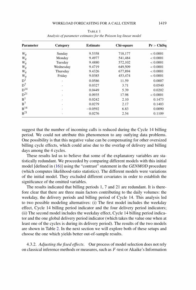
TABLE 1Analysis of parameter estimates for the Poisson log-linear model
Parameter Category Estimate Chi-square Pr > ChiSq
Wq Sunday 9.5358 718,177 < 0.0001Wq Monday 9.4977 541,484 < 0.0001Wq Tuesday 9.4880 572,102 < 0.0001Wq Wednesday 9.4719 649,509 < 0.0001Wq Thursday 9.4326 677,894 < 0.0001Wq Friday 9.0385 453,474 < 0.0001
D1 · 0.0586 11.59 0.0007D7 · 0.0327 3.71 0.0540D14 · 0.0449 5.39 0.0202D21 · 0.0935 17.98 < 0.0001B1 · 0.0242 2.10 0.1473B7 · 0.0279 2.17 0.1403B14 · −0.0592 6.83 0.0090B21 · 0.0276 2.54 0.1109
suggest that the number of incoming calls is reduced during the Cycle 14 billingperiod. We could not attribute this phenomenon to any outlying data problems.One possibility is that this negative value can be compensating for other oversizedbilling cycle effects, which could arise due to the overlap of delivery and billingdays among the 4 cycles.
These results led us to believe that some of the explanatory variables are sta-tistically redundant. We proceeded by comparing different models with this initialmodel [defined in (16)] using the “contrast” statement in the GENMOD procedure(which computes likelihood-ratio statistics). The different models were variationsof the initial model. They excluded different covariates in order to establish thesignificance of the omitted variables.
The results indicated that billing periods 1, 7 and 21 are redundant. It is there-fore clear that there are three main factors contributing to the daily volumes: theweekday, the delivery periods and billing period of Cycle 14. This analysis ledto two possible modeling alternatives: (i) The first model includes the weekdayeffect, Cycle 14 billing period indicator and the four delivery period indicators;(ii) The second model includes the weekday effect, Cycle 14 billing period indica-tor and the one global delivery period indicator (which takes the value one when atleast one of the cycles is during its delivery period). The results of the two modelsare shown in Table 2. In the next section we will explore both of these setups andchoose the one which yields better out-of-sample results.
4.3.2. Adjusting the fixed effects. Our process of model selection does not relyon classical inference methods or measures, such as F -test or Akaike’s Information

1420 S. ALDOR-NOIMAN, P. D. FEIGIN AND A. MANDELBAUM
TABLE 2Log-linear models contrasts analyses. Each row depicts a different model which is compared to theinitial model. Comparing models 1 and 2 to the initial model shows that the extra variables are not
significant at a significance level of 5%
Numeratordegrees offreedom
Denominatordegrees offreedom
The alternative modelexplanatory variablesModel no. F Pr > F
1 Weekday, 6 240 1.89 0.0834billing 14 period indicator,global delivery period indicator
2 Weekday, 3 240 2 0.1152billing 14 period indicator,four delivery period indicators
Criteria [Sakamoto, Ishiguro and Kitagawa (1999)]. These methods rely on thelearning-set and its dimension but do not consider the models forecasting qualities.
Therefore, we decide to explore the influence of the models’ elements on theprediction performance based on the 2004 validation-set. The evaluation criteriawere detailed in Section 4.2.
Keeping the parsimony5 concept in mind, Figure 2 suggests that some weekdaypatterns resemble others. Mainly, Monday through Thursday have similar intra-dayperiod profiles. We shall explore two alternatives for the weekday pattern setting:(i) a model which includes a different period profile for each weekday—we re-fer to this setting as the Multi-Pattern setting; (ii) a model which includes threeintra-day patterns (i.e., one for Sunday, one for Friday and one for the rest of theweekdays)—we refer to this setting as the Three-Pattern setting.
Combining the two different settings for the intra-day effects with the two set-tings of the billing cycles effects (detailed in Section 4.3.1) results in four differ-ent models: (i) Model 1—is a Three-Pattern model which also includes Cycle 14billing period and one global delivery period indicator; (ii) Model 2—is a Three-Pattern model which also includes Cycle 14 billing period and four delivery periodindicators; (iii) Model 3—is a Multi-Pattern model which also includes Cycle 14billing period and one global delivery period indicator; (iv) Model 4—is a Multi-Pattern model which also includes Cycle 14 billing period and four delivery periodindicators.
For now, we shall set the between-periods (within-day) correlation structure ac-cording to a first-order autoregressive structure. We choose this specific structurefor its simplicity. In the next section we will also consider other correlation struc-tures. We also fix the value of σ 2 to its 0.25 theoretical value.
5Parsimony refers to the philosophic rule where the simplest of competing theories/models bepreferred to the more complex.

WORKLOAD FORECASTING FOR A CALL CENTER 1421
TABLE 3RMSE results for the three fixed effects models and two benchmarks models
RMSE
N = 203 Model 1 Model 2 Model 3 Benchmark 1 Benchmark 2
1st quartile 31.80 32.28 32.55 33.24 32.39Median 39.30 40.16 40.19 40.54 39.98Mean 44.78 47.19 45.49 46.51 45.453rd quartile 51.63 58.29 52.38 54.88 53.16
In addition, we compare the four models with the performance of the two bench-mark models, mentioned in Section 4.1.3. The first benchmark model only includesthe weekday effect and the weekday period profiles. The alternative benchmarkmodel has the Multi-Pattern fixed effects and two additional billing cycles’ indica-tors: one global delivery indicator and the billing period indicator associated withCycle 14. The reason why these specific fixed effects settings were chosen will beexplained later in this section.
These six models are evaluated using the same out-of-sample prediction proce-dure previously discussed.
We use the SAS®/STAT Mixed procedure in order to implement and evaluate thecandidate models. Convergence problems occurred when we tried to implementModel 4 with the Multi-Pattern and the billing cycles effects. Therefore, this modelwas subsequently excluded from the analysis.
Tables 3, 4, 5 and 6 present the results of the three different fixed model setups.Out of the three different models, the 1st alternative seems to exhibit the best re-sults. Its results are generally better than the benchmark models. One might arguethat the shorter confidence intervals imply that the benchmark models outperformthe first model. However, since their coverage probabilities are very far from thenominal 95%, we conclude that these narrow intervals are unreliable and probablyresult from an underestimated error variance, that is, σ 2
R . This phenomenon can
TABLE 4APE results for the four fixed effects models and two benchmarks models
APE
N = 203 Model 1 Model 2 Model 3 Benchmark 1 Benchmark 2
1st quartile 6.51 6.57 6.74 6.81 6.77Median 8.13 8.45 8.12 8.24 8.09Mean 9.27 9.75 9.41 9.58 9.413rd quartile 11.27 11.75 11.34 11.29 11.31

1422 S. ALDOR-NOIMAN, P. D. FEIGIN AND A. MANDELBAUM
TABLE 5Coverage probabilities for the four fixed effects models and two benchmarks models
Coverage probability
N = 203 Model 1 Model 2 Model 3 Benchmark 1 Benchmark 2
1st quartile 0.92 0.88 0.92 0.33 0.33Median 0.96 0.96 0.96 0.50 0.50Mean 0.93 0.92 0.93 0.49 0.493rd quartile 1 1 1 0.63 0.63
occur when not all of the sources of variability are accounted for in the model and,in particular, when correlation structure in the data is ignored.
The second benchmark model includes the same billing cycles’ settings as thefirst model. It can be thought of as a “fixed” version of the first model, that is,without the random effects. It is interesting to see that introducing the intra- andinter-day correlations generally improves the forecasting results. Intuitively speak-ing, the additional correlation parameters result in wider confidence intervals tocompensate for the extra uncertainty.
Following these analyses, the models considered in the next subsection willall have the fixed effects of the 1st model. These fixed effects include the Three-Pattern intra-day effect and the two indicators of the billing cycles.
4.3.3. Dependence structures. Having chosen the fixed effects that will be in-corporated in our model, we now discuss the modeling of the random effects. Thereare two sources of variation in our model: one is from the daily volume effect γ
and the other is the within-day error vector ε.We begin by examining different structures for the matrix R which is the within-
day covariance matrix where the residuals’ variance (i.e., σ 2) is confined to its the-oretical value of 0.25. Based on previous research [e.g., Avramidis, Deslauriers andL’Ecuyer (2004)], we consider two simple time series structures for R which bothcan account for the strong intra-day correlations. The first is an AR(1) (first order
TABLE 6Confidence interval widths for the three fixed effects models and two benchmarks models
Width
N = 203 Model 1 Model 2 Model 3 Benchmark 1 Benchmark 2
1st quartile 150.03 149.14 149.13 52.62 51.44Median 168.99 169.22 168.81 59.67 58.80Mean 175.47 178.24 174.31 62.92 61.443rd quartile 195.27 194.61 197.81 68.95 67.86

WORKLOAD FORECASTING FOR A CALL CENTER 1423
TABLE 7Different within-day errors covariance structure.
RMSE results
N = 203 RMSE
R covariance structure AR(1) ARMA(1,1)
1st quartile 31.80 31.85Median 39.30 39.36Mean 44.78 44.813rd quartile 51.63 51.26
auto-regressive) implying that ri,j = σ 2R · ρ|i−j |. The second is an ARMA(1,1)
(auto-regressive moving averages) which means that ri,j = σ 2R · δ · ρ|i−j |−1 (the
covariance between periods i and j where i �= j ) and ri,i = σ 2R (which is the
variance of period i). Other covariance structures theoretically may also be in-corporated here, but since most of them are more complex (such as the Toeplitzform, which includes more parameters), we did not consider them because of com-putational limitations. Note also that most other forms of covariance matrices inSAS®/STAT are not directly related to time series structures.
We evaluate and compare the models using the same technique we developedfor selecting the fixed effects. We use the same learning data as before.
The results are shown in Tables 7, 8, 9 and 10. The results for the ARMA(1,1)
show only slight improvements in the coverage probability compared to the AR(1)
structure. However, it seems that the point predictions are slightly better using theAR(1) structure. Another factor that should be taken into consideration is that theCPU time was higher for the ARMA(1,1) model. In conclusion, the model chosenfor R in this approach is the AR(1) model for the residual error vector.
The last source of variability is the daily volume effect, G. We assume that itscovariance structure also has a first-order autoregressive form. This basic assump-tion means that if on a certain day the call center experienced a rise in the amount
TABLE 8Different within-day errors covariance structure.
APE results
N = 203 APE
R covariance structure AR(1) ARMA(1,1)
1st quartile 6.51 6.52Median 8.13 8.12Mean 9.27 9.283rd quartile 11.27 11.20

1424 S. ALDOR-NOIMAN, P. D. FEIGIN AND A. MANDELBAUM
TABLE 9Different within-day errors covariance structure
comparison. Coverage results
N = 203 Coverage probability
R covariance structure AR(1) ARMA(1,1)
1st quartile 0.92 0.92Median 0.96 1Mean 0.93 0.943rd quartile 1 1
of incoming calls (compared to the fixed effects prediction), then we would alsoexpect to see a similar increase during the following days. As the days becomefarther apart from that day, we expect its influence to decline.
We investigated the influence of the γ correlations by comparing our mixedmodel with an alternative model which does not include this random effect. Usingthe company’s current strategy for prediction which includes a relatively long lead-time of one week, one would hardly expect to see any difference between the twomodels. The results are summarized in Tables 11, 12, 13 and 14. The results showa slight improvement after incorporating an AR(1) structure.
To examine the influence of the between-day random effect, we further explorethe results of the above two models by changing the lead-time period. This analysisis presented in Section 4.5. The analysis reveals that the model incorporating theAR(1) inter-day covariance structure produces better results.
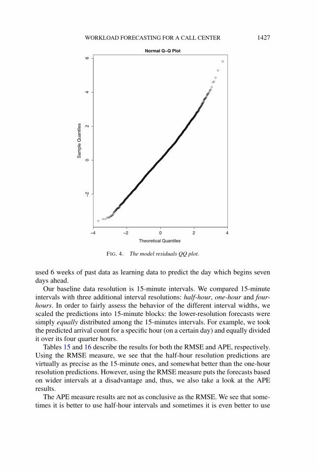
4.3.4. Final model choice—goodness of fit. Our final model includes an intra-day pattern for each weekday, two billing cycles indicators and a first order auto-regressive structure for both the intra-day and the inter-day correlations. Figure 4presents the QQ-plot for the residuals of our final model. It appears that the as-sumption of normally distributed residuals is reasonable.
TABLE 10Different within-day errors covariance structure.
Width results
N = 203 Width
R covariance structure AR(1) ARMA(1,1)
1st quartile 150.03 154.93Median 168.99 174.01Mean 175.47 179.963rd quartile 195.27 204.09

WORKLOAD FORECASTING FOR A CALL CENTER 1425
TABLE 11Testing the influence of the daily random effect. RMSE results
RMSE
Model with AR(1)
daily random effectModel without a
daily random effectN = 203
1st quartile 31.80 31.92Median 39.30 39.67Mean 44.78 44.833rd quartile 51.63 50.40
As mentioned in previous sections, the theoretical value of σ 2, described in (1),is 0.25. We reran our chosen model, but this time we did not specify the value ofσ 2 in advance. Instead we computed the estimated value of this parameter. Sincewe predict 203 days in our database (each time based on 6 weeks data with alead-time of 7 days), we can obtain 203 values of this parameter. Based on thesevalues, the mean estimated value was 0.29. Since the estimated value of σ 2 isclose to 0.25, we are inclined to believe that the model has discovered the majorityof the predictive structure in the data, and that what is left is purely random andunpredictable variation.
4.4. Justifying the half-hour periods. An interesting debate might be held be-tween practitioners and theoreticians as to what is the appropriate interval reso-lution to analyze. Theoreticians might say that in order to fully maintain the ho-mogeneity assumption the intervals should be as small as possible. Alternatively,from a practitioner’s point of view, the resolution should be determined as a func-tion of managerial flexibility: for example, if it is feasible to change the numberof available agents every 5 minutes, then this should be the appropriate intervalresolution. (Such high flexibility can occur, e.g., in large call centers where thereare typically agents who are occupied with various off-line tasks and who can be
TABLE 12Testing the influence of the daily random effect. APE results
APE
Model with AR(1)
daily random effectModel without a
daily random effectN = 203
1st quartile 6.51 6.46Median 8.13 8.15Mean 9.27 9.283rd quartile 11.27 11.09

1426 S. ALDOR-NOIMAN, P. D. FEIGIN AND A. MANDELBAUM
TABLE 13Testing the influence of the daily random effect. Coverage results
Coverage probability
Model with AR(1)
daily random effectModel without a
daily random effectN = 203
1st quartile 0.92 0.88Median 0.96 0.96Mean 0.93 0.923rd quartile 1.00 1.00
made immediately available for service.) However, our experience suggests thatcall centers commonly plan their daily schedule according to either half-hour or15-minute resolutions.
Our Gaussian mixed model can be easily modified to deal with different inter-val resolutions. An interesting question is how much worse are predictions basedon lower-level resolutions than 15-minute predictions, when evaluated at the 15-minute period level. For example, if one predicted accurately the arrival count overa half-hour period, but in that period the first 15 minutes had 0.5 times the aver-age arrival rate, and the second 15 minutes had 1.5 times the average arrival rate,then using the half-hour prediction (by dividing it equally over each 15-minuteinterval) would lead one to seriously overstaff during the first 15 minutes and un-derstaff during the second 15 minutes. This problem would not have happened ifone had good predictions at the 15-minute resolution.
Hence, we are interested in analyzing the effect of the interval resolution on theforecast accuracy at the finest practical resolution.
To this end, we use our Israeli Telecom data and predict the arrival counts be-tween 10 a.m. and 10 p.m. during the 203 regular weekdays between April 11 andDecember 24, 2004. The forecast procedure is the same as before, meaning that we
TABLE 14Testing the influence of the daily random effect. Width results
Width
Model with AR(1)
daily random effectModel without a
daily random effectN = 203
1st quartile 150.03 144.20Median 168.99 163.49Mean 175.47 165.953rd quartile 195.27 186.43
WORKLOAD FORECASTING FOR A CALL CENTER 1427
FIG. 4. The model residuals QQ plot.
used 6 weeks of past data as learning data to predict the day which begins sevendays ahead.
Our baseline data resolution is 15-minute intervals. We compared 15-minuteintervals with three additional interval resolutions: half-hour, one-hour and four-hours. In order to fairly assess the behavior of the different interval widths, wescaled the predictions into 15-minute blocks: the lower-resolution forecasts weresimply equally distributed among the 15-minutes intervals. For example, we tookthe predicted arrival count for a specific hour (on a certain day) and equally dividedit over its four quarter hours.
Tables 15 and 16 describe the results for both the RMSE and APE, respectively.Using the RMSE measure, we see that the half-hour resolution predictions arevirtually as precise as the 15-minute ones, and somewhat better than the one-hourresolution predictions. However, using the RMSE measure puts the forecasts basedon wider intervals at a disadvantage and, thus, we also take a look at the APEresults.
The APE measure results are not as conclusive as the RMSE. We see that some-times it is better to use half-hour intervals and sometimes it is even better to use

1428 S. ALDOR-NOIMAN, P. D. FEIGIN AND A. MANDELBAUM
TABLE 15Prediction accuracy as a function of interval resolution. We compare the RMSE result of the mixed
model for four different resolutions: 15-minute, half-hour, one-hour and four-hour
RMSE
15-minutes Half-hour One-hour Four-hour
Min 12.28 12.07 14.13 32.181st quartile 19.67 19.81 20.86 38.18Median 22.48 22.59 23.56 41.37Mean 24.97 25.06 25.87 42.803rd quartile 28.45 28.29 29.18 46.14Max 60.00 60.01 60.21 73.12
the hour intervals and not the 15-minutes ones. However, it is also noticeable thatthe differences between the three resolutions are usually quite small. The four-hour resolution results are quite bad in comparison with the other interval reso-lutions. These results can be used to justify the use of half-hour intervals in ourcase study—only a minor improvement to precision might be achieved by using ahigher resolution.
In our comparisons, we have used the same AR(1) and ARMA(1,1) autocor-relation structure between periods no matter what their length. (Of course, theparameters were estimated independently for each.) A reviewer has pointed out,it is feasible that allowing a different correlation structure for 15-minute periodsmay achieve better performance than that based on half-hour periods. Due partly tocomputational convergence problems for more complicated correlation structures,these were not considered here.
4.5. Dependence of precision on forecast lead-time. Our prediction processhas three user defined elements: the learning time; the prediction lead-time; and
TABLE 16Prediction accuracy comparison as a function of interval resolution. We compare the APE result of
the mixed model with four different resolutions: 15-minute, half-hour, one-hour and four-hour
APE
15-minutes Half-hour One-hour Four-hour
Min 5.68 5.57 5.36 7.171st quartile 8.01 8.03 8.14 9.74Median 9.30 9.34 9.33 11.20Mean 10.59 10.59 10.67 12.653rd quartile 12.08 12.24 12.15 14.70Max 27.33 27.18 26.84 30.78

WORKLOAD FORECASTING FOR A CALL CENTER 1429
the forecasting horizon. During our model’s training stage we did not change theseparameters.
Academic studies such as Weinberg, Brown and Stroud (2007) and Shen andHuang (2008b) concentrate on producing one-day-ahead predictions or sometimesonline updating forecasting algorithms. These methods, however, do not addressthe industry problem of attaining good predictions in order to produce the weeklyschedule sufficiently ahead of time. Trying to cope with this problem, our TelecomCompany actually uses a two stage process. It first produces a somewhat inaccurate(rough) forecast ten days ahead of the desired week, and then it generates anotherforecast five days before. The second forecast, we are being told, is essential inorder to adequately schedule agents. One interesting question that arises from thispractice is the extent to which prediction lead-time effects forecasting accuracy.
In order to study prediction lead-time effects, we ran our forecasting procedureusing seven different lead times, ranging from one-day-ahead to seven-days-ahead.The learning period and the forecasting horizon stay the same, that is, six weeksand one day, respectively. We ran this prediction procedure using two models:one is with a between-day covariance structure; and one without it (just as we didin Section 4.3.3). This allows us to further examine the effect of this covariancestructure.
We analyzed the prediction results of the two models for each weekday sepa-rately. We do this in order to examine if certain weekdays are more influenced bythe change in forecast lead time.
Figures 5 and 6 present the boxplots of individual RMSEs and APEs for eachweekday, as a function of the forecast lead time.
Surprisingly, the results indicate that shorter lead times do not always improvepredictions’ accuracy. However, it is also important to notice that the differencebetween the lead-time results for each weekday are small for both the APE and theRMSE. This property may be useful for call center managers who want to know ifthey should update their week-ahead forecasts one or two days ahead.
Another conclusion that can be derived is that incorporating the AR(1) inter-day covariance structure generally improves the prediction results. For example,looking at Figures 5 and 6, we can see that the median RMSE and APE6 of themodel with the AR(1) covariance structure generally both have values less than orequal to the median RMSE and APE of the model without it.
5. Modeling expected service times. In addition to predicting arrival rates,forecasting the workload of a queuing system requires also predicting the averageservice patterns (or alternatively the service rate pattern over each day). Since our
6The median is indicated by a black horizontal short line inside the boxplots.

1430 S. ALDOR-NOIMAN, P. D. FEIGIN AND A. MANDELBAUM
FIG. 5. Comparison of RMSE as a function of the prediction lead time. The blue (left) boxplotcorresponds to the model with AR(1) correlation structure between days and the yellow (right)boxplot corresponds to the model without it.

WORKLOAD FORECASTING FOR A CALL CENTER 1431
FIG. 6. Comparison of APE as a function of the prediction lead time. The blue (left) boxplot cor-responds to the model with AR(1) correlation structure between days and the yellow (right) boxplotcorresponds to the model without it.

1432 S. ALDOR-NOIMAN, P. D. FEIGIN AND A. MANDELBAUM
arrival’s model applies a specific resolution (30 minutes), one must predict averageservice times during those same time intervals (periods).
Our model involves two explanatory variables that may affect service rates: theweekday and the period. We compare two alternative models where one is a gen-eralization of the other.
In Figure 3, the average service time patterns resemble a quadratic curve.Hence, the first model describes the average service time using a quadratic re-
gression in the periods, with interactions with the weekday effect, where the periodis included as a numeric variable (rather than as a categorical variable). Intuitivelyspeaking, this model states that the daily service time curves differ among the dif-ferent weekdays but they are confined to be of a quadratic form.
This model formulates the average service time during period k, that is, zdk inthe following manner:
Model 1: zdk = αqd+ β1 · k2 + β2 · k + γ1,qd
· k2
(17)+ γ2,qd
· k + φ · d + εdk; εdk ∼ N(0, σ 2),
where αq is the constant term related to the qth weekday; β1 and β2 are, re-spectively, the quadratic and linear coefficients; γ1,qd
and γ2,qdare the weekday-
specific quadratic and linear period effects and make up the weekday-period inter-action effects. The last effect is a postulated linear daily trend coefficient denotedby φ. We naturally added a random error term denoted by εdk .
The second model is a generalization of the first model and it assumes that theperiod’s variable is a categorial variable. It basically assumes that each weekdayhas its own average service times pattern with no other restriction on its shape.Hence, it is a generalization of the previous quadratic profile model. It is a morecomplicated model which involves many more parameters. We add both the lineardaily trend effect to this model and the error term as well. This model can beformulated in the following manner:
Model 2: zdk = ρqd,k + φ · d + εdk; εdk ∼ N(0, σ 2),(18)
where ρq,k is the interaction between the weekday and the effect of the kth period.We estimate parameters of the two average service times models using the
SAS® GLM procedure. The learning data include dates between mid-February,2004 and the end of December, 2004. Examining the first model results shows thatthe interaction between the quadratic period term and the weekday is not signifi-cant. Consequently, we also examined the first model excluding the insignificantterm. This last model is referred to as Model 3. Since our data has a large numberof observations (6096 which correspond to 254 regular days), we use the asymp-totic log-likelihood ratio chi-square test to compare the models. Table 17 summa-rizes the results of the different models. We compare Model 3 against Model 2 tocheck if the generalized model is significantly better than the reduced quadraticmodel. The relevant chi-square statistic equals 13.524 and the appropriate p-value
WORKLOAD FORECASTING FOR A CALL CENTER 1433
TABLE 17Average service time models. Model 1 assumes a different
quadratic curve for each weekday. Model 3 is the same as Model 1excluding the interaction between the quadratic period term andthe weekday. Model 2 is the generalized model which assumes a
different pattern for each weekday
Model no. No. of parameters Error SS
1 18 588.9072 144 575.8843 13 589.408
is approximately one. It thus seems that the generalized model (i.e., Model 2) isnot significantly better in modeling the average service times. Hence, we chooseModel 3 as our forecasting model.
Figure 7 shows the predicted pattern for each weekday between August 8, 2004and August 13, 2004 versus the true average service times using Models 2 and 3.
By comparing the predictions to the true service means in the same manner aswe did with the arrival process analysis, we calculate the mean APE. Its value is7.68%. The predictions and the mean APE value will later be used to estimatealternative measures of system loads.
6. Forecasting offered-loads in support of staffing. In this section we beginwith a brief review of how we obtained estimators for the expected load using ourdata. We then introduce measures that evaluate the performance of forecasts ofthe offered-load (R) with respect to the QED “square-root staffing” rule. We alsoshow how to use these measures to evaluate the impact of prediction errors (in theoffered-loads) on call center operational performance.
6.1. Estimating expected load. In an Mt/G/N + G queueing system, theoffered-load Rt at time t is defined to be the average number of servers (agents)that would be busy at time t , in the corresponding infinite server system Mt/G/∞(with the same arrival process and same service times). One can show [see, e.g.,Whitt (2007)] that Rt has the following two representations:
Rt = E
∫ t
t−Sλ(u)du = Eλ(t − Se) · ES;(19)
here S is a generic service-time, and Se is a random variable with the stationary-excess cdf associated with the service time cdf G, namely,
Pr(Se ≤ t) ≡ 1
E(S)
∫ t
0[1 − G(u)]du, t ≥ 0.(20)

1434 S. ALDOR-NOIMAN, P. D. FEIGIN AND A. MANDELBAUM
FIG. 7. The predicted average service pattern for typical weekdays as a function of period usingModels 2 and 3. The points represent the (true) estimated average service times. The (blue) dottedline represents the predicted average service times using Model 2 and the (red) line represents theappropriate predictions using Model 3.
The offered-load at time t plays a central role in the planned staffing at thattime, as will be explained in the next section. Whitt (2007) employs Taylor-seriesapproximations to justify the first-order approximation Rt ≈ λ(t −E(Se))E(S). If

WORKLOAD FORECASTING FOR A CALL CENTER 1435
the system reaches a steady-state or if the arrival rate λ is constant, then the offered-load is exactly given by R = λ ·ES. However, under time-varying arrivals, the tworepresentations above demonstrate that staffing at time t must take into accountthe arrivals prior to t (over the stochastic time interval (t − S, t]), which manifestsitself through Whitt’s approximation [the arrival rate λ at time (t − E(Se)].
In our model we assume that the arrival process is an inhomogeneous Poissonprocess but that during each 30-minute interval the arrival rate remains constant.Hence, we predict the offered-load at day d during the kth interval by the followingnatural statistic:
Rdk = λdk · Sdk
30, d = 1, . . . ,D, k = 1, . . . ,K,(21)
where λdk is the predicted arrival count at day d during the kth interval, and Sdk
is the estimated average service time during that same interval. (The division by30 is to convert the predicted arrival rate into the same units as the average ser-vice time—minutes). In concert with the above, we also assume that performanceduring each time interval can be predicted via the queueing model M/G/N + G.
Whitt (2005) shows that, for practical parameter values, the performance of theM/G/N + G model is rather insensitive to the service-time distribution, whereasthe time to impatience distribution has a far greater impact. This reduces perfor-mance analysis to that of the tractable M/M/N +G queue. But, furthermore, in thedesired regimes for call centers’ operations, M/M/N + G can be in fact approxi-mated (with a suitable transformation of parameters) by M/M/N +M (Erlang-A),as articulated in Zeltyn (2005) and Manedelbaum and Zeltyn (2007). These obser-vations will be used in the next section to evaluate system performance.
6.2. Error in β and implications. The square-root staffing rule, described inthe Introduction, gives rise to the so-called Quality and Efficiency Driven (QED)operational regime Gans Koole and Mandelbaum (2003). Here, the number of ser-vice providers (agents), denoted N , is determined by the relation
N = ⌈R + β · √R
⌉,(22)
where R is the offered-load defined previously. The value of β determines a callcenter’s operational regime: it is Quality-Driven with large beta, Efficiency-Drivenwith small, and QED if β is near zero [typically within (−2,1)]. In order to main-tain the latter regime, the system manager strives to achieve a careful balance be-tween service quality and efficiency. For a discussion on how to determine β , as afunction of operating costs (staffing and congestion costs), see Manedelbaum andZeltyn (2007), Zeltyn (2005), Borst, Mandelbaum and Reiman (2004).
Define βu as the user (say, call center manager) chosen β . In order to forecastthe number of required agents, N , the user will use the predicted values of thearrival and service rates to forecast the offered-load, and set
N = R + βu ·√
R,(23)

1436 S. ALDOR-NOIMAN, P. D. FEIGIN AND A. MANDELBAUM
where R is the forecasted offered-load.In practice, the assigned agents will face the true (realized) value (λ) of the
arrival rate and the actual service rate (μ). With these real values of λ, μ, and thecorresponding value of R and the pre-determined number of agents N , the callcenter is in effect operating under a different value of β . This adjusted value of β
will be referred to as βa , which is determined via
βa = N − R√R
.
The above expression can be rewritten as
N = R + βa
√R.(24)
Since the number of pre-assigned agents (N ) is the same in both equations (23)and (24), we can equate them and conclude the following:
R + βa · √R = R + βu ·√
R,
βa − βu ·√
R
R= R − R√
R.
The mean APE for average service time is 0.0768, which means that√
μμ
has a
value of approximately 1. The mean APE arrival rate is 0.0927, indicating that√
λλ
also has a value of approximately 1. Considering these two values, we conclude
that√
RR
≈ 1, which allows us to make the following approximation:
�β � βa − βu≈ R − R√R
.(25)
The quantity �β measures the standardized difference between the predictedoffered-load and the true offered-load. Examining its values can help assess fore-casting quality. It enables one to answer questions such as follows: does this fore-casting algorithm usually overestimate or under-estimate the number of arrivals?;and, by how many agents will one under or overstaff? Note that the ideal value of�β is zero, indicating a perfect point prediction of the realized offered-load.
In Figure 8 we examine the averaged �β values across the 24 periods of theday using our final mixed model predictions. To obtain these averaged values ofthe estimated �β , we first estimate �β for each day in our learning data duringeach period. These were averaged for each period separately over all the days,excluding holidays and irregular days.
Small absolute values of �β (a user’s βu close to the actual βa) indicate thatour model does quite well in predicting the values of offered-load. The estimatedaverage values are close to zero but are usually smaller than zero, which meansthat for most parts of the day the predictions would lead to some under-staffing.
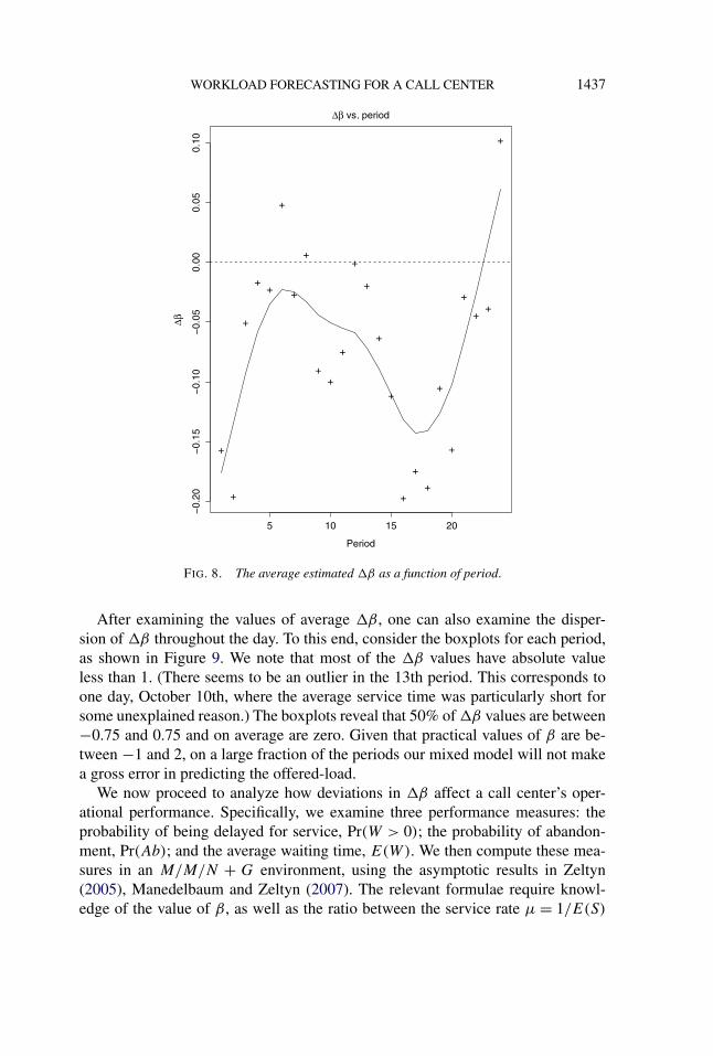
WORKLOAD FORECASTING FOR A CALL CENTER 1437
FIG. 8. The average estimated �β as a function of period.
After examining the values of average �β , one can also examine the disper-sion of �β throughout the day. To this end, consider the boxplots for each period,as shown in Figure 9. We note that most of the �β values have absolute valueless than 1. (There seems to be an outlier in the 13th period. This corresponds toone day, October 10th, where the average service time was particularly short forsome unexplained reason.) The boxplots reveal that 50% of �β values are between−0.75 and 0.75 and on average are zero. Given that practical values of β are be-tween −1 and 2, on a large fraction of the periods our mixed model will not makea gross error in predicting the offered-load.
We now proceed to analyze how deviations in �β affect a call center’s oper-ational performance. Specifically, we examine three performance measures: theprobability of being delayed for service, Pr(W > 0); the probability of abandon-ment, Pr(Ab); and the average waiting time, E(W). We then compute these mea-sures in an M/M/N + G environment, using the asymptotic results in Zeltyn(2005), Manedelbaum and Zeltyn (2007). The relevant formulae require knowl-edge of the value of β , as well as the ratio between the service rate μ = 1/E(S)

1438 S. ALDOR-NOIMAN, P. D. FEIGIN AND A. MANDELBAUM
FIG. 9. Boxplots of �β for the different periods.
and an (im)patience rate parameter θ . [One can think of 1/θ as some measure ofaverage (im)patience.]
We compute performance measures for three values of the ratio between servicerate and patience rate: 0.1—corresponding to impatient customers; 1—averagecustomer patience is the same as their average service time; and 2—implying thatcustomers are rather patient. (Based on our experience, a value of 2 for this ratiois quite realistic.) For further discussion on these issues refer to Zeltyn (2005),Manedelbaum and Zeltyn (2007).
Since �β only provides us with the deviation between βa and βu, we mustdetermine one of them in order to compute the other. Hence, we choose threereasonable values for βu: −1,0,1. Using these values and �β , we can calculateβa . The next step is to compute performance measures using the two different β’s,the predicted offered-load and the observed offered-load. This provides us with thethree performance measures for each period during each day, for βu and βa .
To analyze the outcomes, we averaged each performance measure over the 203days. This provides us with all three average performance measures for each periodusing βu and βa , and for each of the three different settings of the ratio betweenμ and θ . Tables 18 and 19 show the average performance measures for two se-lected periods: the 6th, 13:00–13:30, and the 16th, 18:00–18:30. (When looking
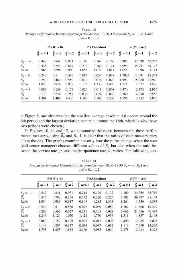
WORKLOAD FORECASTING FOR A CALL CENTER 1439
TABLE 18Average Performance Measures for the period between 13:00–13:30 using βu = −1,0,1 and
μ/θ = 0.1,1,2
Pr(W > 0) Pr(Abandon) E(W) (sec)μθ
= 0.1 μθ
= 1 μθ
= 2 μθ
= 0.1 μθ
= 1 μθ
= 2 μθ
= 0.1 μθ
= 1 μθ
= 2
βu = −1 0.442 0.841 0.931 0.199 0.167 0.160 3.882 32.528 62.223βa 0.428 0.754 0.819 0.210 0.180 0.174 4.099 35.741 69.173Ratio 0.968 0.896 0.900 1.055 1.077 1.087 1.055 1.098 1.111
βu = 0 0.240 0.5 0.586 0.087 0.057 0.047 1.7023 11.091 18.377βa 0.252 0.487 0.550 0.010 0.076 0.070 1.993 15.270 27.94Ratio 1.05 0.974 0.938 0.115 1.333 1.490 1.171 1.377 1.520
βu = 1 0.083 0.159 0.179 0.024 0.011 0.008 0.476 2.173 2.975βa 0.113 0.224 0.257 0.038 0.024 0.020 0.760 4.850 8.558Ratio 1.361 1.409 1.436 1.583 2.182 2.500 1.596 2.232 2.876
at Figure 8, one observes that the smallest average absolute �β occurs around the6th period and the largest deviation occurs at around the 16th, which is why thesetwo periods were chosen.)
In Figures 10, 11 and 12, we summarize the ratios between the three perfor-mance measures, using βa and βu. It is clear that the ratios of each measure varyalong the day. The graphs examine not only how the ratios change when the user(call center manager) chooses different values of βu but also when the ratio be-tween the service rate, μ, and the (im)patience rate, θ , varies. The following con-
TABLE 19Average Performance Measures for the period between 18:00–18:30 βu = −1,0,1 and
μ/θ = 0.1,1,2
Pr(W > 0) Pr(Abandon) E(W) (sec)μθ = 0.1 μ
θ = 1 μθ = 2 μ
θ = 0.1 μθ = 1 μ
θ = 2 μθ = 0.1 μ
θ = 1 μθ = 2
βu = −1 0.442 0.841 0.931 0.214 0.179 0.172 4.100 34.355 65.716βa 0.475 0.798 0.854 0.172 0.230 0.225 5.182 46.597 91.144Ratio 1.05 0.989 0.917 0.804 1.285 1.308 1.264 1.356 1.387
βu = 0 0.240 0.5 0.586 0.092 0.060 0.0501 1.764 11.606 19.229βa 0.299 0.562 0.627 0.131 0.105 0.098 2.666 21.556 40.434Ratio 1.246 1.124 1.070 1.424 1.750 1.956 1.511 1.857 2.103
βu = 1 0.083 0.159 0.179 0.025 0.012 0.008 0.490 2.255 3.095βa 0.149 0.295 0.337 0.054 0.037 0.032 1.116 7.699 13.395Ratio 1.795 1.855 1.883 2.160 3.083 4.000 2.278 3.414 4.328

1440 S. ALDOR-NOIMAN, P. D. FEIGIN AND A. MANDELBAUM
FIG. 10. The average waiting probability ratio over periods. Each of the three plots has threecurves. Each curve corresponds to a different βu value (i.e., −1,0,1). The plots examine the ratio ofthe average waiting probabilities using βa and βu. The three plots, from left to right, show the resultswhen using ratios of μ
θ = 0.1, μθ = 1 and μ
θ = 2, respectively.
clusions can be drawn from the graphs and tables:
• The average waiting probability ratios show more variability for higher valuesof βu. However, when we examine the average waiting probability ratios acrossdifferent ratios of μ and θ , there is little variation.
FIG. 11. The average abandonment probability ratio over periods. Each of the three plots has threecurves. Each curve corresponds to a different βu value (i.e., −1,0,1). The plots examine the ratio ofthe average abandonment probabilities using βa and βu. The three plots, from left to right, show theresults when using ratios of μ
θ = 0.1, μθ = 1 and μ
θ = 2, respectively.

WORKLOAD FORECASTING FOR A CALL CENTER 1441
FIG. 12. The average waiting time ratio over periods. Each of the three plots has three curves.Each curve corresponds to a different βu value (i.e., −1,0,1). The plots examine the ratio of theaverage waiting time using βa and βu. The three plots, from left to right, show the results when usingratios of μ
θ = 0.1, μθ = 1 and μ
θ = 2, respectively.
• The average abandonment probability ratios vary more for higher values of βu,and also for higher values of the ratio between μ and θ . From the tables we seethat the probabilities of abandonment are not large (usually smaller than 0.1).
• The average waiting time ratios vary more for higher values of βu and this isalso true for higher values of the ratio between μ and θ . From the tables we seethat the average waiting times are not long (usually less than 1 minute).
6.3. Error in number of servers. The actual error in the number of servers,due to forecasting error, is also of interest. Using the same methodology as before,one can assume that β has been chosen to achieve specified quality and efficiencygoals. Then, based on the predicted values R of the true offered-load R, the numberof required agents N is estimated via
N = R + β ·√
R.(26)
Knowing the true offered-load, R, the appropriate number of agents is N—thecorrect number of agents required to handle the actual system load at the desiredquality and efficiency trade-off. Formally,
N = R + β · √R.(27)
From the above two formulae and the conclusions that were derived in Section 6.2,one deduces the following relations:
�N � N − N ≈ R − R ≈ �β · √R.(28)

1442 S. ALDOR-NOIMAN, P. D. FEIGIN AND A. MANDELBAUM
FIG. 13. The average estimated �N as a function of period.
The measure �N enables one to evaluate the difference between the actuallydeployed and the desired number of agents.
We proceed with calculating �N , using the same data as before. Figure 13demonstrates the results.
Not surprisingly, the outcomes are quite similar to the graphs we observed whenexamining �β . We are underestimating the offered-load and hence under-staffingthe call center. However, the deviation between the required and the predictednumber of agents for most periods is less than 1 agent, which is encouraging.This seems to indicate that our prediction models offer a rather good solution forestimating the offered-load in the QED regime.
6.4. Lead-time effect. In Section 4.5 we examined the effect of forecast leadtime on the precision of arrival counts predictions. The analysis revealed that theforecast lead time has no significant influence on precision. Now we would liketo examine how the forecast lead time affects �β and �N . Intuitively, one wouldexpect both of these measures to decrease in their absolute value as we shortenlead times.
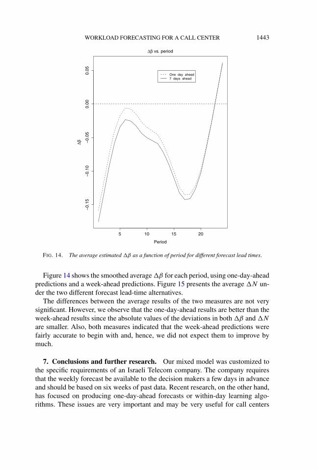
WORKLOAD FORECASTING FOR A CALL CENTER 1443
FIG. 14. The average estimated �β as a function of period for different forecast lead times.
Figure 14 shows the smoothed average �β for each period, using one-day-aheadpredictions and a week-ahead predictions. Figure 15 presents the average �N un-der the two different forecast lead-time alternatives.
The differences between the average results of the two measures are not verysignificant. However, we observe that the one-day-ahead results are better than theweek-ahead results since the absolute values of the deviations in both �β and �N
are smaller. Also, both measures indicated that the week-ahead predictions werefairly accurate to begin with and, hence, we did not expect them to improve bymuch.
7. Conclusions and further research. Our mixed model was customized tothe specific requirements of an Israeli Telecom company. The company requiresthat the weekly forecast be available to the decision makers a few days in advanceand should be based on six weeks of past data. Recent research, on the other hand,has focused on producing one-day-ahead forecasts or within-day learning algo-rithms. These issues are very important and may be very useful for call centers
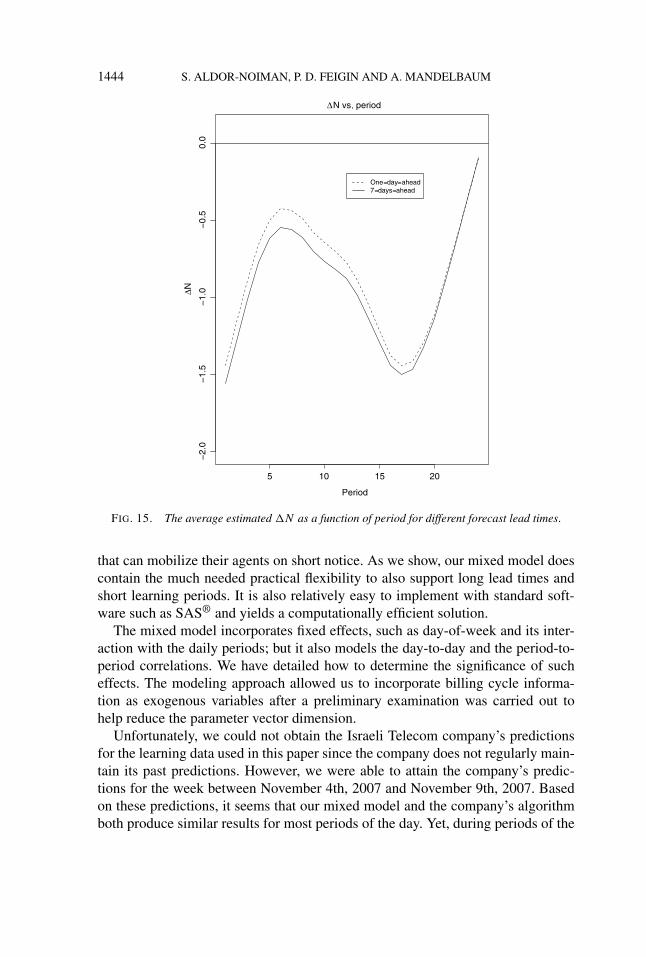
1444 S. ALDOR-NOIMAN, P. D. FEIGIN AND A. MANDELBAUM
FIG. 15. The average estimated �N as a function of period for different forecast lead times.
that can mobilize their agents on short notice. As we show, our mixed model doescontain the much needed practical flexibility to also support long lead times andshort learning periods. It is also relatively easy to implement with standard soft-ware such as SAS® and yields a computationally efficient solution.
The mixed model incorporates fixed effects, such as day-of-week and its inter-action with the daily periods; but it also models the day-to-day and the period-to-period correlations. We have detailed how to determine the significance of sucheffects. The modeling approach allowed us to incorporate billing cycle informa-tion as exogenous variables after a preliminary examination was carried out tohelp reduce the parameter vector dimension.
Unfortunately, we could not obtain the Israeli Telecom company’s predictionsfor the learning data used in this paper since the company does not regularly main-tain its past predictions. However, we were able to attain the company’s predic-tions for the week between November 4th, 2007 and November 9th, 2007. Basedon these predictions, it seems that our mixed model and the company’s algorithmboth produce similar results for most periods of the day. Yet, during periods of the

WORKLOAD FORECASTING FOR A CALL CENTER 1445
day which exhibit more instability (mainly early morning and late evening), theiralgorithm performs worse than our mixed model.
The mixed model results were examined under different lead times. From apractical perspective, a manager might wish to consider a two-stage predictionforecast: first, producing an early weekly forecast for the scheduling process; andnext, producing another forecast one day before the week begins. This later pre-diction might provide a more reliable forecast. Using this one-day-ahead forecast,the manager of a call center might be able to incorporate immediate changes intothe weekly schedule.
We investigated the interval resolution effect on the prediction accuracy. Thisanalysis showed that, for practical implementations, one can use a half-hour reso-lution with only little loss to the prediction accuracy levels. Using this resolutioncan simplify the problem when compared with the 15-minute resolution. It is alsoa practical time interval which call center managers often use for determining theirweekly staff schedule.
Our original forecast problem was to predict the system load based on the av-erage service times and the arrival rates. To model the average service times, wesuggested and fitted a fairly easy quadratic regression model which incorporatesweekdays and period effects.
Having both the average service times’ predictions and the arrival counts, weconstructed QED regime performance measures. Using these measures, we ana-lyzed the effect of our models results on a call center’s operational performance(i.e., the probability of being delayed for service, the probability of abandonmentand the average waiting time). Our results indicate that during busy periods, whenthe QED regime’s “square-root staffing” rule is relevant, the system will performat a desired level commensurate with the actual load or very close to it. This resultgives some evidence that one can ensure a prespecified QED regime using loadforecasts that are sufficiently precise.
An interesting future research question is how to estimate and predict the sys-tem load function R(t) directly (instead of predicting the average service timesand arrival rates separately). Such estimation problems can be approached usingnonparametric methods or parametric models. It will be interesting to learn if suchprediction methods yield better results than the method proposed here. [For furtherdiscussion about the effects of time-varying system load on determining staffinglevels, the reader is referred to Feldman et al. (2008).]
Acknowledgments. The authors thank Professor Larry Brown for proofread-ing and helpful suggestions. We also want to thank a number of reviewers forconstructive comments and suggestions.
SUPPLEMENTARY MATERIAL
Supplement: Israeli Telecom company call center data set and forecastingcode (DOI: 10.1214/09-AOAS255SUPP; .zip). The zip folder contains three files:

1446 S. ALDOR-NOIMAN, P. D. FEIGIN AND A. MANDELBAUM
a readme file which describes the data set in detail; the Israeli Telecom companydata set both in text format and SAS format; and the SAS®/STAT [SAS (2004)]code which was used to create our final forecasting model.
REFERENCES
AKSIN, Z., ARMONY, M. and MEHROTA, V. (2007). The modern call-center: A multi-disciplinaryprespective on operations management research. Production and Operations Management 16465–688.
ALDOR-NOIMAN, S., FEIGIN, P. D. and MANDELBAUM, A. (2009). Supplement to “Workloadforecasting for a call center: Methodology and a case study.” DOI: 10.1214/09-AOAS255SUPP.
ANDREWS, B. H. and CUNNINGHAM, S. M. (1995). L. L. Bean improves call-center forecasting.Interfaces 25 1–13.
ANTIPOV, A. and MEADE, N. (2002). Forecasting call frequency at a financial services call centre.J. Oper. Res. Soc. 53 953–960.
AVRAMIDIS, A. N., DESLAURIERS, A. and L’ECUYER, P. (2004). Modeling daily arrivals to atelephone call center. Management Science 50 896–908.
BORST, S., MANDELBAUM, A. and REIMAN, M. (2004). Dimensioning large call centers. Oper.Res. 52 17–34. MR2066238
BROWN, L. D., GANS, N., MANDELBAUM, A., SAKOV, A., SHEN, H., ZELTYN, S. and ZHAO, L.(2005). Statistical analysis of a telephone call center: A queueing-science prespective. J. Amer.Statist. Assoc. 100 36–55. MR2166068
BROWN, L. D., ZHANG, R. and ZHAO, L. (2001). Root un-root methodology for non parametericdensity estimation. Techical report, The Wharton School, Univ. Pennsylvania.
DEMIDENKO, E. (2004). Mixed Models: Theory and Applications. Wiley, Haifa, Israel. MR2077875FEIGIN, P., MANDELBAUM, A., ISHAY, E., and TROFIMOV, V. (2003). Data MOCCA—Data
MOdel for Call Center Analysis. Technical report, Technion—Israel Institute of Technology.Available at http://iew3.technion.ac.il/ serveng/course2004/References/DataMOCCA.pdf.
FELDMAN, Z., MANDELBAUM, A., MASSEY, W. A. and WHITT, W. (2008). Staffying of time-varying queues to achieve time-stable performance. Management Science 54 324–338. Availableat http://iew3.technion.ac.il/serveng/References/FeldmanMMW020507.pdf.
GANS, N., KOOLE, G. and MANDELBAUM, A. (2003). Telephone call centers: Tutorial, review, andresearch prospects. Manufacturing and Service Operations Management 5 79–141.
GILSON, K. A. and KHANDELWAL, D. K. (2005). Getting more from call centers. The McKinseyQuartely. Available at http://www.evolvondemand.com/download_file_684.pdf.
HENDERSON, C. R. (1975). Best linear unbiased estimation and prediction under a selection model.Biometrics 31 423–447.
HOLMAN, D., BATT, R. and HOLTGREWE, U. (2007). The global call center report: In-ternational perspectives on managment and employment. ILR Collection, Research Stud-ies and Reports, Cornell Univ. Available at http://www.ilr.cornell.edu/globalcallcenter/upload/GCC-Intl-Rept-US-Version.pdf.
JONGBLOED, G. and KOOLE, G. (2001). Managing uncertainty in call centers using Poisson mix-tures. Appl. Stoch. Models Bus. Ind. 17 307–318. MR1873474
MANDELBUAM, A. (2004). Call centers (centres) research bibiliography with abstracts. Chap-ter two details Statistics and Forecasting related papers. Available at http://iew3.technion.ac.il/serveng/References/references.html.
MANEDELBAUM, A. and ZELTYN, S. (2007). Staffing many-server queues with impatient cus-tomers: Constraint satisfation in call centers. Oper. Res. To appear.
MCCULLAGH, P. and NEDLER, J. A. (1989). Generalized Linear Models, 2nd ed. Chapman & Hall,Boca Raton, FL.

WORKLOAD FORECASTING FOR A CALL CENTER 1447
R DEVELOPMENT CORE TEAM (2005). R: A Language and Environment for Statistical Comput-ing. R Foundation for Statistical Computing, Vienna, Austria. ISBN 3-900051-07-0. Available athttp://www.R-project.org.
SAKAMOTO, Y., ISHIGURO, M. and KITAGAWA, G. (1999). Akaike Information Criterion Statistics.Springer, New York.
SAS (2004). SAS OnlineDoc®9.1.3. SAS Institute Inc., Cary, NC.SHEN, H. and HUANG, J. Z. (2005). Analysis of call centre arrival data using singular value decom-
position. App. Stoch. Models Bus. Ind. 21 251–263. MR2159632SHEN, H. and HUANG, J. Z. (2008a). Forecasting time series of inhomogeneous poisson process
with application to call center workforce management. Ann. App. Statist. 2 601–623.SHEN, H. and HUANG, J. Z. (2008b). Interday forecasting and intraday updating of call center
arrivals. Manufacturing and Service Operations Management 10 391–410.SOYER, R. and TARIMCILAR, M. M. (2008). Modeling and analysis of call center arrival data:
A Bayesian approach. Managment Science 54 266–278.TANIR, O. and BOOTH, R. J. (1999). Call center simulation in Bell Canada. In Proceedings of the
1999 Winter Simulation Conference (P. A. Farrington, N. H. B. Nembhard, D. T. Sturrock andG. W. Evans, eds.) 1640–1647. IEEE Press, Piscataway, NJ.
TAYLOR, J. W. (2008). A comparison of univariate time series methods for forecasting intradayarrivals at a call center. Managment Science 54 253–265.
WEINBERG, J., BROWN, L. D. and STROUD, J. R. (2007). Bayesian forecasting of an inhomoge-neous Poisson process with applications to call center data. J. Amer. Statist. Assoc. 102 1185–1199. MR2412542
WHITT, W. (2005). Engineering solution of a basic call-center model. Managment Science 51 221–235.
WHITT, W. (2007). What you should know about queueing models to set staffing requirements inservice systems. Naval Res. Logist. 54 476–484. MR2380781
XU, W. (2000). Long range planning for call centers at Fedex. The Journal of Bussiness ForecastingMethods and Systems 18 7–11.
ZELTYN, S. (2005). Call centers with impatient customers: Exact analysis and many-server asymp-totics of the M/M/N + G queue. Ph.D. thesis, Technion—Israel Institute of Technology. Avail-able at http://ie.technion.ac.il/serveng/References/references.html.
S. ALDOR-NOIMAN
DEPARTMENT OF STATISTICS
THE WHARTON SCHOOL
UNIVERSITY OF PENNSYLVANIA
PHILADELPHIA, PENNSYLVANIA 19104USAE-MAIL: [email protected]
P. D. FEIGIN
A. MANDELBAUM
WILLIAM DAVIDSON FACULTY OF
INDUSTRIAL ENGINEERING AND MANAGEMENT
TECHNION–ISRAEL INSTITUTE OF TECHNOLOGY
TECHNION CITY, HAIFA 32000ISRAEL
E-MAIL: [email protected]@tx.technion.ac.il