workingpaper10 emotions and chat in a financial markets ... · emotions and chat in a financial...
TRANSCRIPT

1
Emotions and Chat in a Financial Markets Experiment
Shaun P. Hargreaves Heap*
Daniel John Zizzo*
University of East Anglia
The Paul Woolley Centre for the Study of Capital Market Dysfunctionality, UTS Working Paper Series 10
Version: March 2011
Abstract This paper examines experimentally two common conjectures in the popular literature on financial markets: that they are swayed by emotion and that they behave like a ‘crowd’. We find consistent evidence that deviations of prices from fundamental value depend on the emotion of excitement and on the presence of independently identified ‘irrational’ traders. Other than through ‘irrational’ traders, there is no evidence, however, that non-price communication (‘chat’) influences prices. Subjects with an economics background make better traders. Keywords: asset bubbles, cheap talk, emotions, noise traders, behavioral finance. JEL Classification Codes: C91, G12.
* CBESS and School of Economics, University of East Anglia, Norwich NR4 7TJ, UK. Email: [email protected]; [email protected]. We thank the Nuffield Foundation and the University of East Anglia for financial support, Richard Wyatt for early discussions and participants at presentations in Gothenburg, London and Nottingham for useful advice. Kei Tsutsui’s research assistance is also gratefully acknowledged. The usual disclaimer applies. The experimental instructions, and other supplementary material, can be found at http://www.uea.ac.uk/~ec601/FinemEApp.pdf.

2
1. Introduction
It is commonly suggested in the popular and historical literature that financial markets
are influenced by waves of emotions (e.g., Smith, 1967, Galbraith, 1994, and Kindleberger,
1996). Markets are subject to ‘waves of optimistic and pessimistic sentiment’ is how Keynes
(1936, p.154), for example, expressed this thought. There is also support for this conjecture
from recent econometric studies (e.g., Baker and Wangler, 2006, Cornelli et al., 2006, and
Edmans et al., 2007).
The approach employed in this paper is different: namely, we try to identify the effects
of emotions on financial markets in a controlled laboratory experiment. This is important not
only because, in general, experiments provide a potentially complementary empirical test to
the econometric one, but also because, in this instance, the experimental approach has an
advantage over the econometric in a significant respect. The observations on sentiment in the
econometric studies are indirect. They are typically other price related variables (like the
discount on closed end funds and the relation between grey prices and actual launch prices
for IPOs) and so naturally raise questions of interpretation. In contrast, the experimental
method potentially allows direct observations on the traders’ or potential traders’ emotional
states, and so it is complementary to the existing econometric evidence in this specific sense.
There has been no previous experimental test of this emotional hypothesis as far as we
are aware of. This is perhaps not so surprising because eliciting the emotional state from
subjects might in itself change behavioral responses, a case of ‘experimenter demand effect’
(Zizzo, 2010). The design of our experiment provides a mechanism for controlling for this
possible effect. We discuss this in the next section.
The experiment is also distinguished by the way that it addresses another, related
conjecture in the popular and historical literature: that the behavior of financial markets is
like that of a ‘crowd’ (see Smith, 1967). A key ingredient of this argument turns on the way
that there is significant non-price communication between traders and potential traders in
financial markets. There are, for instance, famous watering holes where traders meet at the
end of the day, Bloomberg chat rooms and the like as well as the public reflection on what is
happening that occurs through media coverage of markets. This matters on this account

3
because the opportunity for communication between people in a ‘crowd’ (particularly of
emotional states) leads people to behave differently than they would as a set of isolated
individuals. Von Schiller’s dictum (cited in Galbraith, 1994, p. 1) makes the point compactly:
“Anyone taken as an individual is tolerably sensitive and reasonable—as a member of a
crowd, he at once becomes a blockhead.”
We examine specifically whether the scope for online chat actually affects behavior in
our experimental market. There is experimental evidence on the influence of such cheap talk
in other games, where it often (and somewhat surprisingly from a game theoretic point of
view) affects behavior (see Farrell and Rabin, 1996, for a discussion and Cooper et al., 1989,
and Camerer, 2003, for some of the evidence). It has not been examined, however, in a
financial markets experiment, although, again, there is some suggestive and insightful
econometric evidence (see Brown et al., 2008).
Section 2 reviews our experimental hypotheses and design. Section 3 presents our
results. We find that there is evidence that emotions affect price but no evidence that the
opportunity for chat generally influences price. There is evidence, however, that the number
of, independently identified, ‘irrationals’ in the market affects the degree of mispricing and
that this influence is greatest when there is chat. It is commonly argued that financial markets
may be affected by the variety of types of traders (e.g. the presence of ‘noise’ traders in De
Long et al, 1990) and our result on the influence of ‘irrationals’ provides a further particular
example of this. We discuss these two key results further in Section 4, where we consider
more broadly the plausibility of all our results regarding the individual characteristics that
appear to affect prices and emotions in our experiment. Section 5 concludes.
2. Experimental design
The experiment was conducted in November and December 2009 at our university.1
Apart from the experimental instructions and a control questionnaire, the experiment was
fully computerized. The experiment was programmed and conducted with the software z-
Tree (Fischbacher, 2007). Almost all subjects were university students, from a wide variety
of subject backgrounds. A total of 216 subjects participated in the 36 sessions. Subjects were 1 The experimental instructions are provided at http://www.uea.ac.uk/~ec601/FinemEApp.pdf.

4
randomly seated in the laboratory. Computer terminals were partitioned to avoid
communication by facial or verbal means. Subjects read the experimental instructions and
answered a control questionnaire, to check understanding of the instructions, before
proceeding with the tasks. They were advised individually if any answers in the
questionnaires were incorrect. The experiment used ‘experimental points’ as currency,
converted into U.K. pounds at the rate of 200 points per pound. The average payment was
£20.70 for an experiment that lasted around 1 1/2 hour.
Subjects played two stages, each with 15 market trading periods of 3 minutes each, plus
a few end of experiment tasks that will be described later in this section. The trading periods
closely followed Smith et al.’s (1988) double auction trading environment. In this trading
environment subjects have an endowment of assets and experimental points and they can
trade the asset, which yields an uncertain dividend in each period, through a double auction
mechanism over 15 periods in the knowledge a) that each period’s dividend, in experimental
points, is a random draw from (0, 8, 28, 60) and b) that the terminal value of the asset is 0. At
the beginning of each stage subjects were equally divided across 3 possible asset and
money/point endowment combinations: 225 points and 1 asset; 585 points and 2 assets; 945
points and 3 assets. This follows exactly design 4 in table 1 of Smith et al. (1988, p.1126).
The virtue of this set-up is that it has been widely used and it readily generates price bubbles,
so there is a backdrop of experimental results that act as a check on our results and an aid
with their interpretation. There were 6 subjects in each session (i.e. two per endowment type)
and there were 9 different sessions in each treatment.
Experimental treatments. We have four experimental treatments that enable us to test
our hypotheses singly and jointly in a 2 x 2 factorial design crossing two dimensions: the
presence of between rounds emotion elicitation and the presence of a chat facility for traders.
(Insert Table 1 about here.)
Treatment 1 in Table 1 is the baseline treatment without either between rounds emotion
elicitation or a chat facility. We have 3 further treatments (numbers 2,3 and 4 below) that test
for the influence of emotions and non-price communication in a 2x2 set up, as set out below.
Emotions Elicitation. In the emotions elicitation treatments (2 and 4 in Table 1), at the
beginning of each period and before trading starts, subjects were asked to rate the extent to

5
which they felt one of four emotions, on a Likert scale between 0 (no emotion) and 7 (high
intensity of the emotion). Subjects were advised that there were no right or wrong answers.
The types of emotion were drawn from Bosman and van Winden’s (2002) study, and were
anger, anxiety, excitement and joy. We chose anger and excitement because they are two
emotions that have been associated with optimism in relation to the future (see Lerner et al,
2003,), and anxiety because it is typically related to pessimism (e.g. see Norem and Cantor,
1986). Joy is distinct from excitement, but is included here because, as another positive
emotion, it provides balance to the two so-called negative emotions of anger and anxiety.
The emotional state questions create a potential experimenter demand effect (Zizzo,
2010) in the sense that the act of asking may either make these feelings more prominent in
subjects’ minds (or possibly less prominent under the interpretation that expression allows a
form of discharge of the emotion). This approach to the elicitation of emotions is deliberately
minimal. However, in so far as there is such an effect and the elicitation of emotions
influences behavior, then the two effects will be revealed in a difference in the behavior of
prices between Treatments 1 and 3 on the one side and treatments 2 and 4 on the other side. If
there is no difference, then either there is no demand effect and/or emotions do not affect
behavior. To test for the latter possibility, we can examine whether prices are related to the
emotional states in the treatment sessions where we have elicited observations on them
through our questions. If the actual emotional states are not related to price, then there
remains the possibility of a demand effect but it no longer matters because there is no
evidence that emotional states (whether affected by our questions or not) affect prices.
Alternatively if emotional states are related to prices in these treatments’ sessions, then we
can conclude that there was no demand effect because a demand effect should then have
produced a difference between the treatments with and without emotion elicitation.
Chat. The Chat treatments (3 and 4 in Table 1) are characterized by the presence of an
option to enter and participate in an anonymous online chat facility. In principle this allows
for non-price communication and, even if not exactly like being in a le Bon ‘crowd’, the
comparison between treatments with and without Chat enables to identify whether chat
communication makes a difference to behavior.

6
End of experiment tasks. At the end of the experiment we had four behavioral tasks
presented in randomized order to try to measure risk aversion, loss aversion, ambiguity
aversion, sensitivity experimenter demand and a measure of subjects’ ‘irrationality’ as
explained below. They corresponded to (a) a standard Holt and Laury (2002) questionnaire in
the domain of gains; (b) an equivalent task in the domain of losses; (c) an ambiguity aversion
task; and (d) a sensitivity to experimenter demand task. The tasks details are provided in
Appendix A. The number of times subjects choose the safer option can be taken as a measure
of risk attitude in task (a). Task (b) consisted in a set of choices between risky options as in
(a), but framed in terms of losses rather than in gains; we combine task (a) choices of the
safer option with task (b) choices of the riskier option to get a proxy for degree of loss
aversion.2 In addition, we test for subjects’ ‘rationality’ through the questions in Tasks (a)
and (b). In these questions, there is one option that clearly financially dominates the other
regardless of the degree of risk aversion or loss aversion. If the subject selects the worse
option in relation to either of these questions, we designate them as ‘irrational’.
Task (c) followed the lead of Engle-Warnick and Laszlo (2006) and offered a choice
between an increasingly ambiguous lottery and the same lottery disambiguated but at a price
in terms of lower expected value. The number of times subjects went for the unambiguous
measure can be used as a measure of ambiguity aversion. Task (d) presented an option
between two lottery choices, one increasingly dominated by the other; the dominated option
was characterized by a smiley face and a sentence stating that “it would be nice if some of
you were to choose” such an option. The nudge provided towards choosing the dominated
lotteries was significant by the standard of what we know about experimenter demand
characteristics (see Zizzo, 2010), with the smiley face providing a social cue to interpret the
sentence of encouragement.3 As a result, we measure the degree of sensitivity to
experimenter demand, which we refer to as ‘conformism’ below, as the number of dominated
options choices being made.
2 A loss averse subject would be risk loving in the domain of losses while being risk averse in the domain of gains. 3 Note that we could not say that “it would be nice if all of you were to choose” the dominated option, since this sentence would in fact have been deceptive given our experimental goals (the usefulness of the measure is in having a distribution of subjects based on the measure).

7
Payments. The average payment was £20.70 for an experiment that lasted around one
and a half hours. The average payment came from three sources: the terminal holdings of
experimental points in the market game (£13.17), a payment for some Holt-Laury tasks
(£5.72) and a show up fee (£2).
3. Results
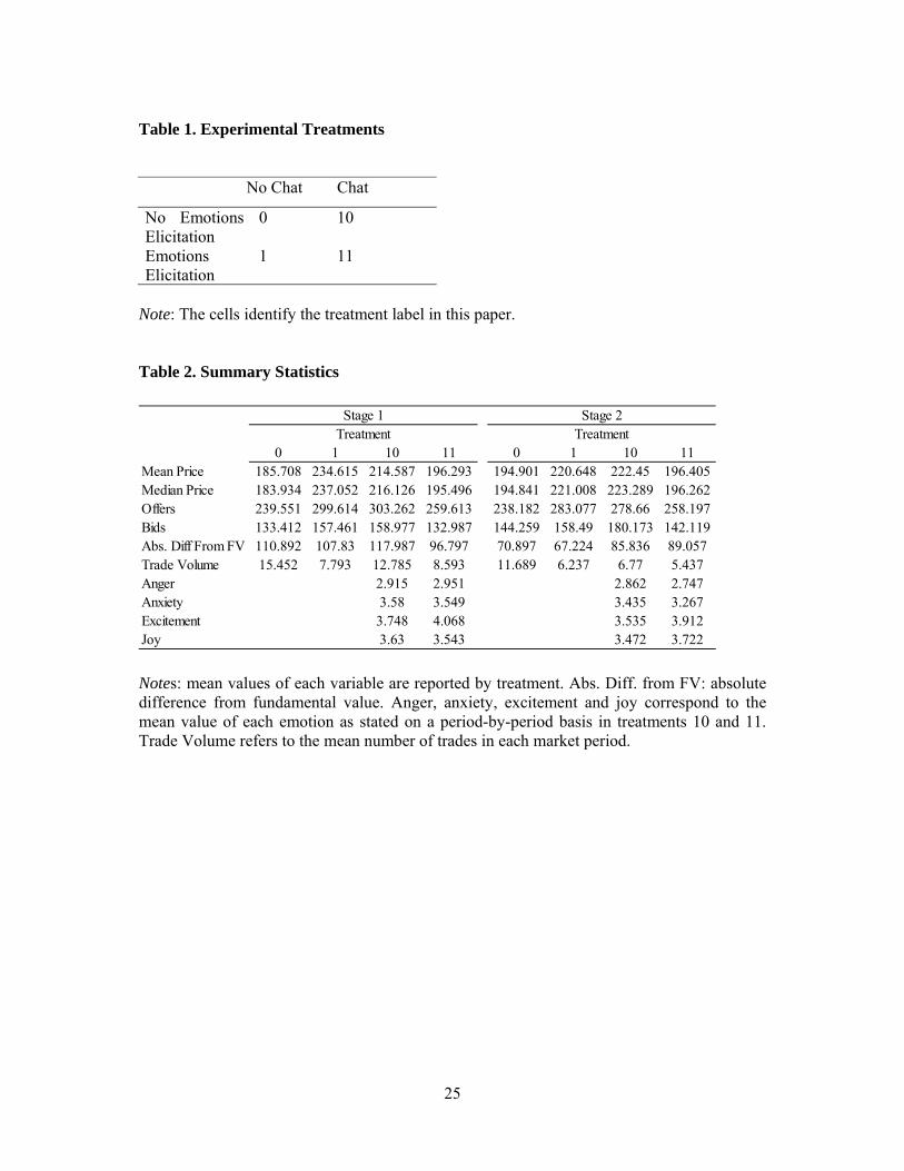
A descriptive summary picture of prices by period for each treatment is given in Figure
1, and more summary information is provided in Table 2.
(Insert Figure 1 and Table 2 about here.)
The results at this level are similar to those found in the literature in the sense that we
reproduce the bubble like behavior for prices and so we have no reason on these grounds to
suppose that there is anything unusual about our implementation. Mean and median prices
roughly coincide and there are also no obvious ‘eyeball’ differences in prices across
treatments. The latter is confirmed by nonparametric tests4 regarding price variables (e.g.,
Kruskal Wallis P = 0.360 and 0.252 in relation to mean and median prices);5 it is also
confirmed by running these tests on just stage 1 or stage 2 data (e.g., in relation to mean and
median prices in stage 2, Kruskal Wallis P = 0.451 and 0.567, respectively). Results do not
change if one pools data depending on whether there is an emotion elicitation mechanism or
not or depending on whether there is a chat mechanism or not (e.g., in relation to mean
prices, Mann-Whitney P = 1.000 in the former case and Mann-Whitney P = 0.527 in the latter
case). There are also no significant differences in price related variables between stage 1 and
2 (e.g. Wilcoxon P = 0.793 in relation to mean prices). These results provide preliminary
evidence that emotions elicitation does not per se change behavior in financial markets,
therefore ruling out the presence of experimenter demand effects connected to such
elicitation. They also provide preliminary evidence against the presence of chat mattering for
trading. The one qualification to this is that there is some suggestive evidence that the volume
of trade decreased as the result of the chat facility (Mann-Whitney P = 0.054), but this is
unsurprising as subjects had something else to do (other than trading) in the Chat treatments. 4 All nonparametric tests referred to in this section are run using each session as the unit of observation, therefore ensuring the independence of observations. 5 The closest to significance we get is in relation to mean bids (Kruskal Wallis P = 0.079).

8
Just around 15% of the subjects (33 out of 216) were ‘irrational’ in the sense of making Holt
and Laury variants choices inconsistent with strict dominance, as discussed in section 2.
Looking at the emotions data, excitement is stated to be the emotion that subjects felt
the most, ahead of joy, anxiety and anger (Wilcoxon P = 0.013, P = 0.015 and P < 0.001
respectively), and with anger clearly as the emotion stated as being the least felt (Wilcoxon P
= 0.002 relative to both joy and anxiety).
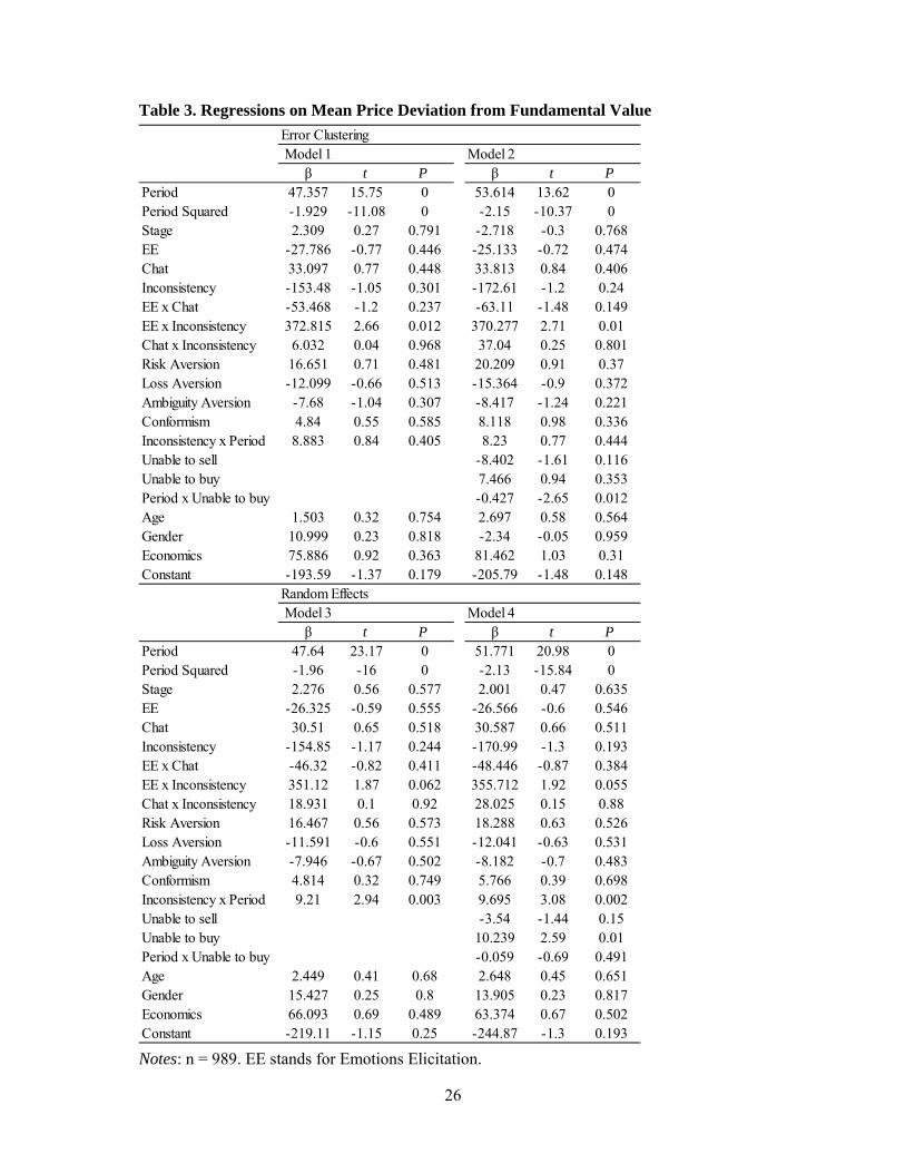
Regressions on prices relative to fundamental value. To investigate the data in more
depth, we conducted regression analysis on the mean price deviation (Table 3) and the
absolute price deviation (Table 4) from fundamental value. We report on both these
possibilities because we have no prior view as to whether treatment differences might be
revealed in one aspect of price behavior in relation to fundamental values or the other (i.e.
absolute or actual deviation). The mean deviation may be easier to interpret in terms of prices
becoming higher or lower relative to fundamental value due to any given factor, but absolute
deviation is what matters in identifying whether such factor helps making the market more or
less efficient. For each set of dependent and independent variables we present two
estimations, one using error clustering and the other using random effects, as both are
commonly used in estimations of this kind (and again we have no prior strong view as to
which technique should be preferred). Either way, we control for the session level non
independence of observations.
(Insert Tables 3 and 4 about here.)
In Models 1, 3, 5 and 7, the independent variable include treatment dummies (EE = 1 in
emotion elicitation treatment, Chat = 1 in treatments with chat opportunities), time variables
(Stage = 1 in stage 2, period refers to trading period number), psychological variables
(Inconsistency = the % of subjects who made ‘irrational’, i.e. strictly dominated choices, in
the Holt and Laury variant tasks; mean Risk Aversion, Loss Aversion, Ambiguity Aversion
and Conformism values measured from the Holt and Laury variant tasks, see Appendix A for
details) and demographic variables (mean Age; Gender = % of female traders; Economics =
% of traders with an economics background). Models 2, 4, 6 and 8 add three variables trying
to identify the effects of being constrained either in terms of not having units to sell (Unable
to sell: number of traders unable to sell) or in terms of being less likely to be able to buy

9
(Unable to buy: number of traders with less cash than fundamental value). For all models
some interaction terms are also included.6
A key result in Table 1 is that, in all cases, neither of the treatment dummies EE and
Chat are significant, either on their own or interacted with each other. EE x Inconsistency
however is positive and statistically significant (P < 0.05 in all models except Models 3 and
4, where P < 0.07): in the emotions elicitations treatments, ‘irrational’ subjects mis-valued
and apparently over-valued the assets. Average mispricing was by around 250 points, which
is considerable given that the average fundamental value was 192 points for each unit of the
asset.
RESULT 1: There is no evidence that the elicitation of emotions generally affects
prices, although it may in relation to ‘irrational’ traders.
RESULT 2: There is no evidence that giving subjects the opportunity for chat directly
affects prices.
There is evidence from the random effects regressions that ‘irrationals’ may have
increased the mean gap between prices and the declining fundamental value as the
experiment progressed (P < 0.01), possibly through inertia in trading rather than tracking
changes in fundamental value, but these effects are not robust to the regression estimation
method. A higher proportion of female traders led to higher price mispricing (P < 0.05),
while there is no other robust result linked to individual characteristics, including our
measure of conformism. That the usual attributes of individuals (e.g. degree of risk aversion)
are not significant might appear surprising but it is also a common finding in the empirical
literature (see Warneryd, 1996, and Guth et al., 1997).
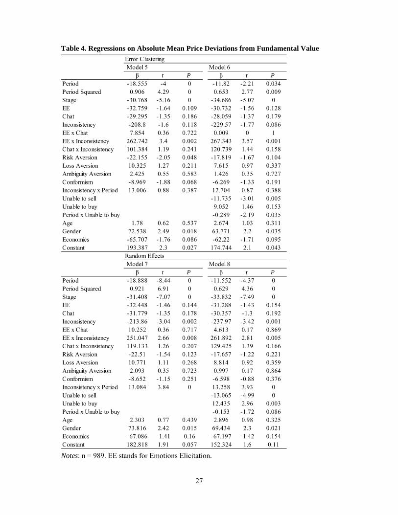
Period and Period Squared are significant (P < 0.05 or better) and that this is so is
clearly connected to the time pattern in the trading that we observed in Figure 1. Models 1-4
identify a traditional dynamic bubble shape in prices as per Figure 1. Models 5-8 show that
6 Period x Unable to sell may not be included because of collinearity, so only Period x Unable to buy is included.

10
there is an initial decline in the absolute gap from fundamental value (Period has a negative
coefficient), though one that tends to level down with time (Period Square has a positive
coefficient). While we are not concerned here with this bursting bubble aspect of price
behavior in the experimental market that is picked up by these ‘period’ terms, we
nevertheless test whether one common explanation of this also holds in our data: a change in
the composition of traders that is occasioned by buying and selling constraints (e.g., Hong
and Stein, 2007). This, in turn, may explain market mispricing.
To elaborate, there may be a range of views among traders along the optimism-
pessimism spectrum and in the early stages of these experiments the ‘optimists’ typically buy
from ‘pessimists’. This action, however, tends to both constrain the ‘optimists’ (because they
run out of liquidity) and the ‘pessimists’ (because they run out of assets to sell). As a result
the balance between optimists and pessimists changes in the market, with consequent effects
for the price. We examine this explanation in Models 2, 4, 6 and 8, which contain the
constrained buyers and sellers variables. The picture from Models 2 and 4 is unclear in terms
of effects on mean price deviations: ‘Unable to buy’ has a positive coefficient (but P = 0.01
in Model 4 only), suggesting that on average optimism may lead to constrained buyers; while
‘Period x Unable to buy’ is negatively signed (but P < 0.02 in Model 2 only), suggesting that,
as the optimists become less able to act on their optimism, prices fall back. The results from
Models 6 and 8 are stronger in terms of effects on the degree of overall mispricing of the
asset. Given the declining fundamental value of the asset, a higher proportion of pessimists
(high ‘Unable to sell’) correlates with lower mispricing (P < 0.01 in both models); a higher
proportion of optimists (high ‘Unable to buy’) might correlate with higher mispricing, though
this effect is sensitive to the estimation method (P = 0.153 in Model 6 and P < 0.01 in Model
8); while, as optimists become less able to act on their optimism, prices become less mis-
valued (P < 0.05 in Model 6 and P < 0.1 in Model 8).
RESULT 3: There is some evidence that price mispricing is related to changes in the
number of traders who are liquidity and short selling constrained.

11
Result 1 suggests that either that there is no experimenter demand effect in general
and/or that emotions have no effect on behavior.7 To examine whether there is evidence of
the latter, we now focus on treatments 1 and 11 (i.e. those where we have observations on the
emotional states of the subjects).
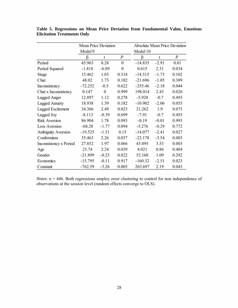
(Insert Table 5 about here.)
Table 5 includes regressions on mean price deviations and absolute mean price
deviations from fundamental values restricted to these treatments, so as to enable us to
include mean emotional values variables: Lagged Anger, Lagged Anxiety, Lagged
Excitement and Lagged Joy. Mean emotional values are measured at period t to predict price
deviations at period t + 1, to ensure that they may be interpreted in causal terms. We find that
random effects regression estimates converge to OLS in this sub-sample,8 but error clustering
can still be used to control for any potential non independence of observations at the sessions
level and this is what we do in Table 5.
It appears that excitement leads to price increases relative to fundamental value (P <
0.05 in Model 9). The effect is large: excitement was measured between 0 and 7 and this
means that an increase in excitement from 0 to 7 would lead to a price increase effect of as
many as about 34 x 7 = 238 points. To put this in perspective, and as noted earlier, the
average fundamental value of a unit of the asset was 192 points. This, in turn, might lead to
some systematic mispricing relative to fundamental value (P < 0.08). There is also some
potential effect of anxiety in making prices closer to fundamental value (P < 0.06).
RESULT 4: There is evidence that excitement raises prices relative to fundamental
value.
Table 5 is also useful in another respect: by having fine-grained information on
emotional states and controlling for them, we can more precisely hope to identify the effects
of psychological characteristics. There is clear evidence that ‘irrationals’ behave differently:
putting together the negative Inconsistency (P < 0.05) and positive Inconsistency x Period (P 7 The possible exception relates to the 15% of ‘irrational’ traders, and will be discussed in the next section. 8 Put it differently, under random effects estimation zero variance is explained by the session level random coefficients;

12
< 0.01) coefficients in Model 10, the picture is one in which ‘irrationals’ are initially much
closer to fundamental value but after around period 5 they misprice the asset progressively
more as ‘irrationals’ fail to track the declining fundamental value.9 ‘Irrationals’ also
systematically misprice the asset more as a result of the chat mechanism, and by a sizeable
amount of around 200 points (P < 0.05 in Model 10).10
Interestingly, conformists misprice less (P < 0.01 in Model 10), and, given the positive
coefficient on Conformism in Model 10 (P < 0.05), this appears to operate by reducing
valuations below fundamental value. Ambiguity aversion also appears to lead to less
mispricing (P < 0.05 in Model 10): the more the ambiguity aversion, the less the likely
demand for the asset may be. We also find that having more traders with an Economics
background leads to prices clearly more aligned with fundamental value (P < 0.05 in Model
10).
RESULT 5: Controlling for emotional state, there is evidence that ‘irrational’ traders
fail to track declining the fundamental value and misprice the asset more as a result of the
chat mechanism.
RESULT 6: Controlling for emotional state, there is evidence that, the higher the
proportion of conformist, ambiguity averse and economics trained traders, the lower the
mispricing.
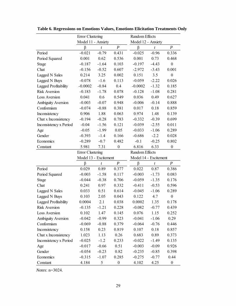
Regressions on emotional state. Result 4 shows that excitement leads to rises in prices
relative the fundamental value, and we also saw from Model 10 that anxiety also potentially
has an effect on market prices. One question that arises is what determines excitement and
anxiety in our financial market, and Table 6 presents regression analysis attempting, at least
partially, to answer this question.11
(Insert Table 6 about here.)
9 Suggestive complementary evidence for this is provided by the marginally significant positive coefficient on Inconsistency x Period in Model 9 (P < 0.07). 10 We shall discuss this in section 4. 11 For completeness, we report equivalent regressions for anger and joy in Appendix B.

13
The unit of observation in these regressions is the emotional value stated by any given
subject in any given market period of any given session. We control for subject level non
independence of observations by using either error clustering or random effects, while we
control for session level non independence by the means of fixed effects. The variables are
the same as before if defined at the subject level where appropriate,12 but we now add Lagged
N Sales and Lagged N Buys, which are respectively the number of sold or bought units in the
previous period by a subject; and Lagged Profitability, which are the profits made by the
subject in the previous period. If we focus on P < 0.05 or better coefficients using both
estimation methods, we find that anxiety rises with sales, while excitement increases with
purchases. It is also interesting that excitement may be rising as a result of past profits, but
the effect is somewhat sensitive to the estimation method (P < 0.05 in Model 13 but P =
0.178 in Model 14).
RESULT 7: Buying assets is connected to excitement and selling assets is connected to
anxiety.
(Insert Table 7 about here.)
Regressions on profitability. We conclude our analysis by considering the possible
determinants of individual profits in our experiment. Table 7 reproduces subjects level
regression on mean profits. As in the case of Table 5, random effects regression estimates
here collapse to OLS and so only error clustering can be used to control for any potential non
independence of observations at the sessions level. Model 15 employs all subjects, while
Model 16 adds mean emotional states (Mean Anger, Mean Anxiety, Mean Excitement and
Mean Joy) to the independent variables and so is restricted to the treatments with emotions
elicitation.13 Mean emotional states do not affect how much money subjects make; but
irrationals do make less money on average (P < 0.02). There is also evidence that female
12 For example, Economics will simply be a dummy equal to 1 if the subject has an Economics background and 0 otherwise, rather than the proportion of subjects with an Economics background in the given session 13 By construction – namely, the zero-sum nature of trading in the market -, each session is equally profitable and so treatment dummies are omitted (though adding them would not affect the regression results).

14
traders make less money (P < 0.05 in Model 15 and P < 0.08 in Model 16). Other effects lack
robustness between Model 15 and 16.
RESULT 8: ‘Irrationals’ make less profits, while subjects’ emotional states do not
affect their own profits.
4. Discussion
These results, taken at face value, are important in at least two respects. First, they
provide the first, as far as we aware, experimental support for the popular conjecture that
financial markets are moved by emotions. Specifically, we find that excitement increases the
mean gap between prices and fundamental value (Result 4). This is plausible since
excitement is connected to optimism; and, in this way, the experiment helps corroborate those
arguments and the econometric evidence that link over-pricing to optimism (see Baker and
Wangler, 2006).
Our method for identifying this emotional influence turns on an experimental design
where we can test for a ‘demand effect’. The introduction of emotions elicitation per se does
not change prices in general, though it may make a difference for ‘irrational’ traders (Result
1). It is the lack of a general ‘demand effect’ that enables us to test for the influence of
specific emotions in those treatments where they are elicited. The possible exception of the
‘irrationals’, though, points to the second important feature of our results. We find that the
number of independently identified ‘irrational’ traders has a distinct influence on prices.
The financial literature has discussed the implications of having noise traders (e.g.,
Shleifer and Summers, 1990, and De Long et al., 1990) and the presence of such traders is
consistent with the evidence in Haruvy and Noussair’s (2006) financial market experiment.
Our results offer a different but essentially complementary development to this line of
argument. Once we put Results 1, 5 and 8 together, it is clear that ‘irrational’ traders – as
defined by performance in tasks independent from market behavior – are indeed different in
our experiment. Emotions elicitation affects ‘irrational’ traders, and so does having a chat
mechanism once emotional states are controlled for. Furthermore, the effects are potentially
quite large: mispricing is of the order of 200-250 points as a result of either factor with a

15
small proportion of ‘irrationals’, and this is over 100% of the average fundamental value of
the financial asset.
The influence of ‘irrationals’ might be explained in more than one way. Asking for
emotional states may make ‘irrational’ traders more dependent on emotional responses. This
is a form of experimenter demand effect with potentially wider scope since it suggests that in
times where traders are more likely to think emotively - such as in time of crisis -, ‘irrational’
traders may indeed lead to greater asset mispricing. An alternative explanation could be that
adding the emotions elicitation task adds to the complexity of the decision environment: this
could make the ‘irrationals’ more prone to confusion and less likely to track fundamental
value, contributing in turn to the speculative bubble observed in this and other asset market
experiments.
The potential role of chat with ‘irrational’ traders is also interesting and can be
interpreted in at least two ways. It could be that ‘irrational’ traders exemplify Schiller’s
dictum and are swayed by the wisdom of the crowd (or lack thereof) and therefore to this
extent – and bearing in mind that ‘irrational’ traders make up only 15% of all traders – there
is some truth in the potential of rumors to induce asset mispricing. Alternatively, it is again
also possible that the chat mechanism adds to the complexity of the decision environment and
so may make ‘irrational’ traders misprice more.
Either way, it is clear that ‘irrational’ traders in our experiment do make less profits
than other traders, and so they pay for their mispricing (Result 8). This does not contradict
noise trader models because the definition of noise trader there (e.g., De Long et al., 1990)
differs from the inconsistency in choices that we have used to identify our ‘irrational’ traders.
The question we now address briefly is whether these results should be taken, in this
way, at their face value. In particular, does what else went on in the experiment make broad
sense, lending credence to these particular results?
Controlling for emotional state, the evidence on the influence of the other individual
characteristics is perhaps the most mixed: i.e. the higher the proportion of conformist,
ambiguity averse and economics trained traders, the lower the mis-pricing (Result 6).
Conformism might have been expected to operate in the reverse way once mis-pricing has
occurred. That ambiguity aversion may lead to less mispricing may also seem surprising as it

16
has been argued that ambiguity lovingness can be treated as an index of competence
(Barberis and Thaler, 2003). However, it seems also plausible to argue that the ambiguity
averse are less likely to engage in trade when prices depart significantly from the known
stochastic process governing fundamental values. And it is unsurprising that an economics
background contributes to better trading because economics could either make better traders
or attract the better traders as a field of study.14
In the same vein, the overall behavior of prices is broadly reassuring, as are the results
on the determinants of emotions and individual profitability. The fact that our asset markets
produced bubbles that are not very different from those found in the literature, for instance,
means that there is no obvious ground for thinking that our experiment was in some way
atypical. Equally the support in our data for a common explanation of these asset prices
bubbles, namely the changing composition of traders due to liquidity and short selling
constraints, adds credence. That women make less profits has also been found elsewhere (e.g.
see Gneezy et al, 2003, where it arises from the fact of competition). Finally, the apparent
determinants of the reported emotions (Result 7) are plausible. Excitement is connected to
optimism and buying assets, while anxiety is connected to pessimism and selling assets. 15
5. Conclusion
Introducing emotions elicitation in our experiment enabled us to identify a large effect
that excitement has on mispricing. When controlling for emotional states, we were further
able to identify the role of several psychological characteristics, including the role of
‘irrational’ traders, who were independently identified using Holt and Laury (2002) type
tasks.
The first of these results is important and new. It is important because it lends support
to a part of the popular (as compared with rational choice) view of financial markets and it is
new because, while there is some econometric support for this bit of popular wisdom, it has
14 These possibilities parallel those considered by Frey and Meier (2005) in evaluating whether economics students are less cooperative; in that context, they find that less cooperative agents tend to study economics rather than that economics make agents less cooperative. 15 The absence of a time pattern to these emotional states is also reassuring in relation to possible endogeneity (i.e., the variation in these emotions does not map on to the time pattern of prices relative to fundamental values).

17
not previously been examined in a controlled environment where emotional states can be
directly measured. The second result builds on this insight in a way that complements the
analyses of financial markets that turn on the presence of a variety of types of traders (e.g. De
Long et al, 1990). In particular, a relatively small percentage (15%) of ‘irrational’ traders
account for a large part of the mispricing in our experiment. We also find some evidence that
the ‘irrationals’ are more susceptible to emotional suggestion and that their mispricing is
greatest when given the opportunity for chat. In other words, while markets are quite
generally moved by emotions in our experiment, it is the behavior of a small group of
‘irrationals’ that is most ‘crowd’ like. Obviously, further research is needed.
References
Baker, Malcolm and Jeffrey C. Wurgler. 2007. “Investor sentiment in the stock market”,
Journal of Economic Perspectives, 21(2), 129-152.
Barberis, Nicholas and Richard Thaler. 2003. “A survey of behavioral finance” in G.
Constantinides, M. Harris, and R. Stulz (Editors) Handbook of the Economics of
Finance, Elsevier, Amsterdam.
Bosman, Ronald, and Frans van Winden. 2002. “Emotional hazard in a power-to-take
experiment.” Economic Journal, 112(476), 147-169.
Brown, Jeffrey, R., Zoran Ivković, Paul A. Smith and Scott Weisbenner. 2008. “Neighbors
matter: Causal community effects and stock market participation”, Journal of Finance,
63(3), 1509-1531.
Camerer, Colin C. (2003) Behavioral Game Theory. Princeton: Princeton University Press.
Cooper, Russell, Douglas V. DeJong, Robert Forsythe and Thomas W. Ross, 1989,
“Communication in the Battle of the Sexes game: Some experimental results”, Rand
Journal of Economics, 20(4), 568-87.
Cornelli, Francesca, David Goldreic and Alexander Ljungqvist. 2006. “Investor sentiment
and pre-IPO markets”, Journal of Finance, 61(3), 1187-121.
De Long, J. Bradford, Andrei Shleifer, Lawrence H. Summers and Robert J. Waldmann.
1990. “Noise trader risk in financial markets”, Journal of Political Economy, 98(4),
703-738.

18
Edmans, Alex, Diego García and Øyvind Norli. 2007. “Sports sentiment and stock returns”,
Journal of Finance, 62(4), 1967-1998.
Engle-Warnick, Jim and Sonia Laszlo, 2006. “Learning-by-doing in an ambiguous
environment”, Mc Gill University Department of Economics working paper, 2006s-29.
Epstein, Larry and Martin Schneider. 2008. “Ambiguity, information quality, and asset
pricing“, Journal of Finance, 63(1), 197-228.
Farrell, John and Mathew Rabin. 1996. “Cheap talk”, Journal of Economic Perspectives
10(3), 103–118.
Fischbacher, Urs, 2007. “z-Tree: Zurich toolbox for ready-made economic experiments”,
Experimental Economics, 10(2), 171-178.
Frey, Bruno, S. and Stephan Meier. “Selfish and indoctrinated economists?” European
Journal of Economics, 19(2), 165-171.
Galbraith, Kenneth. 1994. A Short History of Financial Euphoria. London: Penguin Books.
Gneezy, Uri, Muriel Nierdele and Aldo Rustichini. 2003. “Performance in competitive
markets: gender differences”, Quarterly Journal of Economics, 118(3), 1049-1074.
Guth, Werner, Jan P. Krahnen and Christian Rieck. 1997. “Financial markets with
asymmetric information: A pilot study focussing on insider advantages”, Journal of
Economic Psychology, 18(2-3), 235-57.
Holt, Charles A. and Laury, Susan K. 2002. “Risk aversion and incentive effects”, American
Economic Review, 92(5), pp. 1644-55.
Hong, Harrison and Jeremy C. Stein. 2007. “Disagreement and the stock market”, Journal of
Economic Perspectives, 21(2), 109-128.
Keynes, John, M. 1936. The General Theory of Employment Interest and Money. London:
Macmillan.
Kindleberger, Charles. 1996. Manias, Panics and Crashes: a History of Financial Crises.
Basingstoke: Macmillan.
Lerner, Jennifer, Roxana M. Gonzalez, Deborah A. Small, and Baruch Fischhoff. 2003.
“Effects of fear and anger on the perceived risks of terrorism: a national field
experiment”, Psychological Science, 14(2), 144-150.

19
Norem, Julie K and Nancy Cantor. 1986. “Defensive pessimism: harnessing anxiety”,
Journal of Personality and Social Psychology, 51(6), 1208-1217.
Rabin, Matthew and Richard Thaler. 2001. “Anomalies: Risk aversion”, Journal of Economic
Perspectives, 15(1), 219-232.
Shleifer, A. and Lawrence H. Summers. 1990. “The noise trader approach to finance”,
Journal of Economic Perspectives, 4(2), 19-33.
Smith, Adam. 1967. The Money Game. New York: Random House.
Smith, Vernon L., Gary L. Suchanek and Arlington W. Williams. 1988. “Bubbles, crashes
and endogenous expectations in experimental spot asset markets”, Econometrica,
56(60), 1119-52.
Warneryd, Karl-Eric. 1996. “Risk attitudes and risky behaviour”, Journal of Economic
Psychology, 17(6), 749-770.
Zizzo, Daniel J. 2010. “Experimenter demand effects in economic experiments”,
Experimental Economics, 13(1), 75-98.
Appendix A The individual task screens were presented in random order, and the order of the columns (i.e., which of the set of lottery choices was to the left and which one was to the right) was randomized. Option labels for the first individual task screen were A and B, those for the second individual task screen were C and D, and so on. (The name of the tasks below is for convenience only, and was not provided to the subjects). Without loss of generality, formulas are provided below with respect to the specific sample computer displays provided in Figures A1 through A4. Risk aversion screen (Insert Figure A1 here.) Index of risk aversion = number of Option A choices in Decisions 1 through 9 In Decision 10, no matter the degree of risk aversion (or indeed loss aversion, as discussed below), subjects should clearly prefer Option B to Option A. Loss Aversion screen (Insert Figure A2 here.)

20
Index of loss aversion = number of Option A choices in Decisions 1 through 9 (as per Figure A1) – (10 – Option H choices in Decisions 1 through 9) In Decision 10, no matter the degree of risk aversion or loss aversion, subjects should clearly prefer Option G to Option H. Loss aversion usually refers to the way that losses are weighed in the utility function representation of choice much more heavily than are the equivalent gains (i.e. the U function is steeper in the loss domain than in the gain domain). This could be consistent with conventional risk aversion but as Rabin and Thaler (2001) has argued, given the small changes in wealth that are typically at stake, the typical observations of double weighting of losses compared with gains would entail quite implausible risk aversion when grossed up to some of the bigger decisions that we make. Hence, loss aversion is more usually thought to denote a kink in the U function at the point of the status quo (and the related inference that we make judgments about changes in wealth and not its absolute level). Whichever interpretation, however, the concept of loss aversion turns on the difference in slope of U function at the point of the status quo. If one assumes that U function representation of choice has a constant coefficient of relative risk aversion ‘r’ as in U = (1/1-r) X(1-r) then a) the slope of U function = X-r and so larger absolute value of ‘r’ means smaller slope for given wealth X and b) an interval can be established for ‘r’ from the switch point S in the Holt and Laury type choice between ‘safe’ and ‘risky’ options. In particular, if the decisions are ordered from 1= decision with the lowest expected value to 10 = decision with the highest expected value, then the inferred value of r increases as the switch point (S) increases (that is slope falls as S increases). Define S(gain) as the switch point in the domain of gains and S(loss) as the switch point in the domain of losses. Then S(gain) – S(loss) is a measure of change in slope of U function between gains domain and loss domain and the hypothesis of loss aversion is that it is positive: that is, the slope is bigger in losses (i.e, r is smaller) than in gains. In Figure A2, however, the decisions in losses are reverse ordered: that is, Decision 1 has the highest expected value and Decision 10 the lowest. Define the switch point when decisions in losses are reverse ordered as S’. Then S(loss) = 10-S’ and so our measure of change in slope can be computed as follows: S(gain) – S(loss) = S(gain) –(10-S’) = number of Option A choices in Decisions 1 through 9 – (10 - number of Option H choices in Decisions 1 through 9). Ambiguity aversion screen (Insert Figure A3 here.) Index of ambiguity aversion = number of Option D choices This is similar to Engle-Warnick and Laszlo (2006) and offers a choice between an increasingly ambiguous lottery and the same lottery disambiguated but at a price in terms of lower expected value. The number of times subjects went for the unambiguous measure can be used as a measure of ambiguity aversion. Conformism screen

21
(Insert Figure A4 here.) Index of conformism = number of Option F choices The two options in Decision 1 are the same, but thereafter Option E improves and Option F worsens. Option F is identified by the smiley face and the note that it would be nice if this was chosen and so is taken to be what conforming with expectations of others, and specifically of the experimenter, would entail. So, as the cost of conformity rises as the number of Option F choices increases, the number of Option F choices can be taken as an index of how conformity is valued.

22
Figure 1. Mean and Median Prices by Treatment

23
Figure A1. Gain Task
Figure A2. Loss Task

24
Figure A3. Ambiguity Aversion Task
Figure A4. Conformism Task
25
Table 1. Experimental Treatments No Chat Chat
No Emotions Elicitation
0 10
Emotions Elicitation
1 11
Note: The cells identify the treatment label in this paper. Table 2. Summary Statistics
0 1 10 11 0 1 10 11Mean Price 185.708 234.615 214.587 196.293 194.901 220.648 222.45 196.405Median Price 183.934 237.052 216.126 195.496 194.841 221.008 223.289 196.262Offers 239.551 299.614 303.262 259.613 238.182 283.077 278.66 258.197Bids 133.412 157.461 158.977 132.987 144.259 158.49 180.173 142.119Abs. Diff From FV 110.892 107.83 117.987 96.797 70.897 67.224 85.836 89.057Trade Volume 15.452 7.793 12.785 8.593 11.689 6.237 6.77 5.437Anger 2.915 2.951 2.862 2.747Anxiety 3.58 3.549 3.435 3.267Excitement 3.748 4.068 3.535 3.912Joy 3.63 3.543 3.472 3.722
Stage 1 Stage 2TreatmentTreatment
Notes: mean values of each variable are reported by treatment. Abs. Diff. from FV: absolute difference from fundamental value. Anger, anxiety, excitement and joy correspond to the mean value of each emotion as stated on a period-by-period basis in treatments 10 and 11. Trade Volume refers to the mean number of trades in each market period.
26
Table 3. Regressions on Mean Price Deviation from Fundamental Value
Error ClusteringModel 1 Model 2
β t P β t PPeriod 47.357 15.75 0 53.614 13.62 0Period Squared -1.929 -11.08 0 -2.15 -10.37 0Stage 2.309 0.27 0.791 -2.718 -0.3 0.768EE -27.786 -0.77 0.446 -25.133 -0.72 0.474Chat 33.097 0.77 0.448 33.813 0.84 0.406Inconsistency -153.48 -1.05 0.301 -172.61 -1.2 0.24EE x Chat -53.468 -1.2 0.237 -63.11 -1.48 0.149EE x Inconsistency 372.815 2.66 0.012 370.277 2.71 0.01Chat x Inconsistency 6.032 0.04 0.968 37.04 0.25 0.801Risk Aversion 16.651 0.71 0.481 20.209 0.91 0.37Loss Aversion -12.099 -0.66 0.513 -15.364 -0.9 0.372Ambiguity Aversion -7.68 -1.04 0.307 -8.417 -1.24 0.221Conformism 4.84 0.55 0.585 8.118 0.98 0.336Inconsistency x Period 8.883 0.84 0.405 8.23 0.77 0.444Unable to sell -8.402 -1.61 0.116Unable to buy 7.466 0.94 0.353Period x Unable to buy -0.427 -2.65 0.012Age 1.503 0.32 0.754 2.697 0.58 0.564Gender 10.999 0.23 0.818 -2.34 -0.05 0.959Economics 75.886 0.92 0.363 81.462 1.03 0.31Constant -193.59 -1.37 0.179 -205.79 -1.48 0.148
Random EffectsModel 3 Model 4
β t P β t PPeriod 47.64 23.17 0 51.771 20.98 0Period Squared -1.96 -16 0 -2.13 -15.84 0Stage 2.276 0.56 0.577 2.001 0.47 0.635EE -26.325 -0.59 0.555 -26.566 -0.6 0.546Chat 30.51 0.65 0.518 30.587 0.66 0.511Inconsistency -154.85 -1.17 0.244 -170.99 -1.3 0.193EE x Chat -46.32 -0.82 0.411 -48.446 -0.87 0.384EE x Inconsistency 351.12 1.87 0.062 355.712 1.92 0.055Chat x Inconsistency 18.931 0.1 0.92 28.025 0.15 0.88Risk Aversion 16.467 0.56 0.573 18.288 0.63 0.526Loss Aversion -11.591 -0.6 0.551 -12.041 -0.63 0.531Ambiguity Aversion -7.946 -0.67 0.502 -8.182 -0.7 0.483Conformism 4.814 0.32 0.749 5.766 0.39 0.698Inconsistency x Period 9.21 2.94 0.003 9.695 3.08 0.002Unable to sell -3.54 -1.44 0.15Unable to buy 10.239 2.59 0.01Period x Unable to buy -0.059 -0.69 0.491Age 2.449 0.41 0.68 2.648 0.45 0.651Gender 15.427 0.25 0.8 13.905 0.23 0.817Economics 66.093 0.69 0.489 63.374 0.67 0.502Constant -219.11 -1.15 0.25 -244.87 -1.3 0.193
Notes: n = 989. EE stands for Emotions Elicitation.
27
Table 4. Regressions on Absolute Mean Price Deviations from Fundamental Value
Error ClusteringModel 5 Model 6
β t P β t PPeriod -18.555 -4 0 -11.82 -2.21 0.034Period Squared 0.906 4.29 0 0.653 2.77 0.009Stage -30.768 -5.16 0 -34.686 -5.07 0EE -32.759 -1.64 0.109 -30.732 -1.56 0.128Chat -29.295 -1.35 0.186 -28.059 -1.37 0.179Inconsistency -208.8 -1.6 0.118 -229.57 -1.77 0.086EE x Chat 7.854 0.36 0.722 0.009 0 1EE x Inconsistency 262.742 3.4 0.002 267.343 3.57 0.001Chat x Inconsistency 101.384 1.19 0.241 120.739 1.44 0.158Risk Aversion -22.155 -2.05 0.048 -17.819 -1.67 0.104Loss Aversion 10.325 1.27 0.211 7.615 0.97 0.337Ambiguity Aversion 2.425 0.55 0.583 1.426 0.35 0.727Conformism -8.969 -1.88 0.068 -6.269 -1.33 0.191Inconsistency x Period 13.006 0.88 0.387 12.704 0.87 0.388Unable to sell -11.735 -3.01 0.005Unable to buy 9.052 1.46 0.153Period x Unable to buy -0.289 -2.19 0.035Age 1.78 0.62 0.537 2.674 1.03 0.311Gender 72.538 2.49 0.018 63.771 2.2 0.035Economics -65.707 -1.76 0.086 -62.22 -1.71 0.095Constant 193.387 2.3 0.027 174.744 2.1 0.043
Random EffectsModel 7 Model 8
β t P β t PPeriod -18.888 -8.44 0 -11.552 -4.37 0Period Squared 0.921 6.91 0 0.629 4.36 0Stage -31.408 -7.07 0 -33.832 -7.49 0EE -32.448 -1.46 0.144 -31.288 -1.43 0.154Chat -31.779 -1.35 0.178 -30.357 -1.3 0.192Inconsistency -213.86 -3.04 0.002 -237.97 -3.42 0.001EE x Chat 10.252 0.36 0.717 4.613 0.17 0.869EE x Inconsistency 251.047 2.66 0.008 261.892 2.81 0.005Chat x Inconsistency 119.133 1.26 0.207 129.425 1.39 0.166Risk Aversion -22.51 -1.54 0.123 -17.657 -1.22 0.221Loss Aversion 10.771 1.11 0.268 8.814 0.92 0.359Ambiguity Aversion 2.093 0.35 0.723 0.997 0.17 0.864Conformism -8.652 -1.15 0.251 -6.598 -0.88 0.376Inconsistency x Period 13.084 3.84 0 13.258 3.93 0Unable to sell -13.065 -4.99 0Unable to buy 12.435 2.96 0.003Period x Unable to buy -0.153 -1.72 0.086Age 2.303 0.77 0.439 2.896 0.98 0.325Gender 73.816 2.42 0.015 69.434 2.3 0.021Economics -67.086 -1.41 0.16 -67.197 -1.42 0.154Constant 182.818 1.91 0.057 152.324 1.6 0.11
Notes: n = 989. EE stands for Emotions Elicitation.
28
Table 5. Regressions on Mean Price Deviation from Fundamental Value, Emotions Elicitation Treatments Only
Mean Price Deviation Absolute Mean Price DeviationModel 9 Model 10
β t P β t PPeriod 45.963 8.28 0 -14.835 -2.91 0.01Period Squared -1.818 -6.89 0 0.615 2.31 0.034Stage 15.462 1.03 0.318 -14.515 -1.73 0.102Chat 48.02 1.73 0.102 -21.696 -1.05 0.309Inconsistency -72.252 -0.5 0.622 -255.46 -2.18 0.044Chat x Inconsistency 0.147 0 0.999 198.014 2.43 0.026Lagged Anger 12.897 1.12 0.278 -5.928 -0.7 0.493Lagged Anxiety 18.938 1.39 0.182 -10.902 -2.06 0.055Lagged Excitement 34.366 2.49 0.023 21.262 1.9 0.075Lagged Joy -8.113 -0.39 0.699 -7.91 -0.7 0.493Risk Aversion 86.904 1.78 0.093 -0.19 -0.01 0.993Loss Aversion -68.28 -1.77 0.094 -5.276 -0.29 0.772Ambiguity Aversion -19.525 -1.51 0.15 -14.077 -2.41 0.027Conformism 35.463 2.26 0.037 -22.178 -3.54 0.003Inconsistency x Period 27.852 1.97 0.066 43.095 3.53 0.003Age 23.74 2.24 0.039 4.021 0.86 0.404Gender -21.899 -0.23 0.822 52.168 1.09 0.292Economics -15.795 -0.11 0.917 -160.32 -2.51 0.023Constant -762.59 -3.26 0.005 263.697 2.19 0.043
Notes: n = 446. Both regressions employ error clustering to control for non independence of observations at the session level (random effects converge to OLS).
29
Table 6. Regressions on Emotions Values, Emotions Elicitation Treatments Only
Error Clustering Random EffectsModel 11 - Anxiety Model 12 - Anxiety
β t P β t PPeriod -0.021 -0.79 0.431 -0.025 -0.96 0.336Period Squared 0.001 0.62 0.536 0.001 0.73 0.468Stage -0.187 -1.64 0.103 -0.197 -4.43 0Chat -0.156 -0.52 0.607 -2.972 -3.43 0.001Lagged N Sales 0.214 3.25 0.002 0.151 3.5 0Lagged N Buys -0.078 -1.6 0.113 -0.059 -2.22 0.026Lagged Profitability -0.0002 -0.84 0.4 -0.0002 -1.32 0.185Risk Aversion -0.183 -1.78 0.078 -0.128 -1.08 0.281Loss Aversion 0.041 0.6 0.549 0.036 0.49 0.627Ambiguity Aversion -0.003 -0.07 0.948 -0.006 -0.14 0.888Conformism -0.074 -0.88 0.381 0.017 0.18 0.859Inconsistency 0.906 1.88 0.063 0.974 1.48 0.139Chat x Inconsistency -0.194 -0.28 0.783 -0.332 -0.39 0.699Inconsistency x Period -0.04 -1.56 0.121 -0.039 -2.55 0.011Age -0.05 -1.99 0.05 -0.033 -1.06 0.289Gender -0.393 -1.4 0.166 -0.686 -2.2 0.028Economics -0.289 -0.7 0.482 -0.1 -0.25 0.802Constant 5.981 7.31 0 6.816 6.33 0
Error Clustering Random EffectsModel 13 - Excitement Model 14 - Excitement
β t P β t PPeriod 0.029 0.89 0.377 0.022 0.87 0.386Period Squared -0.003 -1.58 0.117 -0.003 -1.73 0.083Stage -0.044 -0.38 0.706 -0.059 -1.35 0.176Chat 0.241 0.97 0.332 -0.411 -0.53 0.596Lagged N Sales 0.033 0.51 0.614 -0.045 -1.06 0.289Lagged N Buys 0.103 2.05 0.043 0.122 4.7 0Lagged Profitability 0.0004 2.1 0.038 0.0002 1.35 0.178Risk Aversion -0.135 -1.21 0.228 -0.082 -0.77 0.439Loss Aversion 0.102 1.47 0.145 0.076 1.15 0.252Ambiguity Aversion -0.042 -0.99 0.323 -0.041 -1.06 0.29Conformism -0.069 -0.88 0.379 -0.064 -0.76 0.446Inconsistency 0.158 0.23 0.819 0.107 0.18 0.857Chat x Inconsistency 1.023 1.13 0.26 0.683 0.89 0.373Inconsistency x Period -0.025 -1.2 0.233 -0.022 -1.49 0.135Age -0.017 -0.66 0.51 -0.003 -0.09 0.926Gender -0.054 -0.23 0.82 -0.235 -0.85 0.398Economics -0.315 -1.07 0.285 -0.275 -0.77 0.44Constant 4.184 5 0 4.102 4.25 0
Notes: n=3024.

30
Table 7. Subject Level Regressions on Profitability
All subjects EE only subjectsModel 15 Model 16
β t P β t PMean Anger -2.277 -0.68 0.496Mean Anxiety 0.928 0.27 0.786Mean Excitement 5.309 0.97 0.331Mean Joy -0.946 -0.19 0.849Inconsistency -17.962 -2.58 0.014 -33.494 -3.05 0.002Risk Aversion 1.64 1.01 0.321 5.912 2.15 0.032Loss Aversion 0.31 0.25 0.806 -0.909 -0.5 0.617Ambiguity Aversion 1.873 2.35 0.025 0.788 0.75 0.456Conformism -1.818 -1.46 0.152 1.967 0.93 0.351Age -0.779 -2.32 0.026 0.053 0.07 0.945Gender -12.876 -2.35 0.024 -13.914 -1.9 0.057Economics 12.33 1.65 0.108 14.217 1.52 0.127Constant 1.864 0.16 0.87 -41.095 -1.45 0.148
Notes: n = 216 (Model 15: all subjects), 108 (Models 16: emotions elicitation treatments only). Both regressions employ error clustering to control for non independence of observations at the session level (random effects converge to OLS).