working with acs - massachusetts institute of...

Working with acs.R

Ezra Haber Glenn, aicpPublic Planning, Research, & Implementation, Inc.

June, 2013

Contents

1 Purpose 2

2 Key Improvements 2

3 Getting Started in R 23.1 Getting and Installing R . . . . . . . . . . . . . . . . . . . . . . . 23.2 Getting and Installing the acs Package . . . . . . . . . . . . . . . 3

3.2.1 Installing from cran . . . . . . . . . . . . . . . . . . . . . 33.2.2 Installing from a zipped tarball . . . . . . . . . . . . . . . 4

3.3 Getting and Installing a Census API Key . . . . . . . . . . . . . 5

4 Working with the New Functions 64.1 Overview . . . . . . . . . . . . . . . . . . . . . . . . . . . . . . . 64.2 User-Specific Geographies . . . . . . . . . . . . . . . . . . . . . . 6

4.2.1 Basic Building Blocks: the single element geo.set . . . . 64.2.2 But where’s the data. . . ? . . . . . . . . . . . . . . . . . . 84.2.3 Real geo.sets: complex groups and combinations . . . . . 84.2.4 Changing combine and combine.term . . . . . . . . . . . 104.2.5 Nested and Flat geo.sets . . . . . . . . . . . . . . . . . . 114.2.6 Subsetting geo.sets . . . . . . . . . . . . . . . . . . . . . . 114.2.7 Two tools to reduce frustration in selecting geographies . 12

4.3 Getting Data . . . . . . . . . . . . . . . . . . . . . . . . . . . . . 164.3.1 acs.fetch(): the workhorse function . . . . . . . . . . . 164.3.2 More descriptive variable names: col.names= . . . . . . . 184.3.3 the acs.lookup() function: finding the variables you want 20

5 Exporting Data 23

6 Additional Resources 24

1

A A worked example using blockgroup-level data and nested com-bined geo.sets 25A.1 Making the geo.set . . . . . . . . . . . . . . . . . . . . . . . . . 25A.2 Using combine=T to make a neighborhood . . . . . . . . . . . . 26A.3 Even more complex geo.sets . . . . . . . . . . . . . . . . . . . . 27A.4 Gathering neighborhood data on transit mode-share . . . . . . . 28

1 Purpose

These notes are intended to accompany the updated acs.R package (version 1.0),developed in partnership with and under contract for Puget Sound RegionalCouncil (PSRC).

2 Key Improvements

Consistent with the scope of services from PSRC, the new version of the acs.R

package includes functions to allow users to create their own geographies bycombining existing ones provided by the Census. In addition to automating theprocess of downloading, importing, and storing data from the American Com-munity Survey for these new geographies (including proper statistical techniquesfor dealing with estimates and standard errors), the package also includes a pairof helpful “lookup” tools, one to help users identify the geographic units theywant, and the other to identify tables and variables from the ACS for the datathey are looking for.

3 Getting Started in R

3.1 Getting and Installing R

R is a complete statistical package—actually, a complete programming lan-guage with special features for statistical applications—with a syntax and work-flow all its own. Luckily, it is well-documented through a variety of tuto-rials and manuals, most notably those hosted by the cran project at htp:

//cran.r-project.org/manuals.html. Good starting points include:

• R Installation and Administration, to get you started (with chapters foreach major operating system); and

• An Introduction to R, which provides an introduction to the language andhow to use R for doing statistical analysis and graphics.

Beyond these, there are dozens of additional good guides. (For a smallsampling, see cran.r-project.org/other-docs.html.)

Exact installation instructions vary from one operating system or distribu-tion to the next, but at this point most include an automated installer of one

2

kind or another (a windows .exe installer, a Macintosh .pkg, a Debian apt

package, etc.). Once you have the correct version to install, it usually requireslittle more than double-clicking an installer icon or executing a single command-line function.

Windows users may also want to review the FAQ at http://cran.r-project.org/bin/windows/base/rw-FAQ.html; similarly, Mac users should visit http:

//cran.r-project.org/bin/macosx/RMacOSX-FAQ.html.

3.2 Getting and Installing the acs Package

3.2.1 Installing from cran

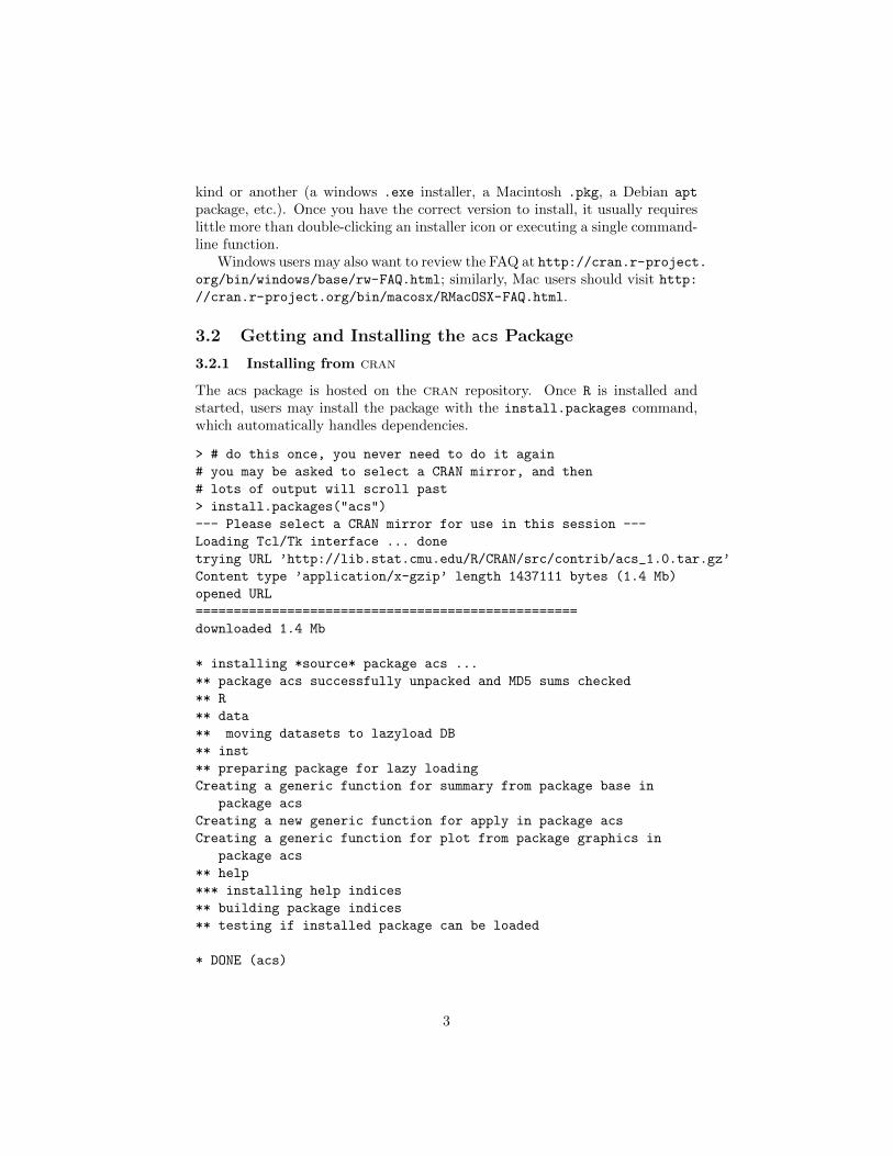
The acs package is hosted on the cran repository. Once R is installed andstarted, users may install the package with the install.packages command,which automatically handles dependencies.

> # do this once, you never need to do it again

# you may be asked to select a CRAN mirror, and then

# lots of output will scroll past

> install.packages("acs")

--- Please select a CRAN mirror for use in this session ---

Loading Tcl/Tk interface ... done

trying URL ’http://lib.stat.cmu.edu/R/CRAN/src/contrib/acs_1.0.tar.gz’

Content type ’application/x-gzip’ length 1437111 bytes (1.4 Mb)

opened URL

==================================================

downloaded 1.4 Mb

* installing *source* package acs ...

** package acs successfully unpacked and MD5 sums checked

** R

** data

** moving datasets to lazyload DB

** inst

** preparing package for lazy loading

Creating a generic function for summary from package base in

package acs

Creating a new generic function for apply in package acs

Creating a generic function for plot from package graphics in

package acs

** help

*** installing help indices

** building package indices

** testing if installed package can be loaded

* DONE (acs)

3

The downloaded source packages are in

/tmp/RtmppeCyGj/downloaded_packages

>

> # once installed, be sure to load the library:

> library(acs)

After installing, be sure to load the package with library(acs) each timeyou start a new session.

3.2.2 Installing from a zipped tarball

If for some reason version 1.0 of the package in not available through the cranrepository (or if, perhaps, you intend to experiment with additional modifi-cations to the version 1.0 source code), we have also provided you with thesoftware as a “zipped tarball” of the complete package. It can be installed justlike any other package, although dependencies must be managed separately.Simply start R and then type:


> install.packages(pkgs = "acs_1.0.tar.gz")

inferring ’repos = NULL’ from the file name

* installing *source* package acs ...

** R

** data

** moving datasets to lazyload DB

** inst

** preparing package for lazy loading

Creating a generic function for summary from package base in

package acs

Creating a new generic function for apply in package acs

Creating a generic function for plot from package graphics in

package acs

** help

*** installing help indices

** building package indices

** testing if installed package can be loaded

* DONE (acs)

>

(You may need to change the working directory to find the file, or specify acomplete path to the pkgs = argument.) Once installed, don’t forget to actuallyload the package to make the installed functions available:

> # do this every time to start a new session

> library(acs)

4

Loading required package: stringr

Loading required package: plyr

Loading required package: XML

Attaching package: acs

The following object(s) are masked from package:base:

apply

>

The acs.R package depends on a few other fairly common R packages: methods,stringr, plyr, and XML. If these are not already on your system, you may needto install those as well—just use install.packages("package.name"). (Note:when the package is downloaded from the CRAN repository, these dependencieswill be managed automatically.)

If installation of the tarball fails, users may need to specify the followingadditional options (likely for Windows and possibly Mac systems):

> install.packages("/path/to/acs_1.0.tar.gz", repos = NULL,

type = "source")

Assuming you were able to do these steps, we’re ready to try it out.

3.3 Getting and Installing a Census API Key

To download data via the American Community Survey application programinterface (API), users need to request a “key” from the Census. Visit http://

www.census.gov/developers/tos/key_request.html and fill out the simpleform there, agree to the Terms of Service, and the Census will email you a secretkey for only you to use.

When working with the functions described below,1 this key must be pro-vided as an argument to the function. Rather than expecting you to providethis long key each time, the package includes an api.key.install() function,which will take the key and install it on the system as part of the package forall future sessions.


> api.key.install(key="592bc14cnotarealkey686552b17fda3c89dd389")

>

1or at least those that require interaction with the API, such as acs.fetch() and thecheck= option for geo.make()—the geo.lookup and acs.lookup functions work fine withouta key, and can even be used when you are off-line.

5

4 Working with the New Functions

4.1 Overview

We’ve tried to make this User Guide as detailed as possible, to help you learnabout the many advanced features of the new package. As a result, it may looklike there is a lot to learn, but in fact the basics are pretty simple: to get ACSdata for your own user-defined geographies, all you need to do is:

1. install and load the package, and (optionally) install an API key (seesections 3.2 and 3.3);

2. create a geo.set using the geo.make() function (see section 4.2);

3. optionally, use the acs.lookup() function to explore the variables youmay want to download (see section 4.3.3 on page 20) ;

4. use the acs.fetch() function to download data for your new geography(see section 4.3.1 on page 16); and then

5. use the existing functions in the package to work with your data (seeworked example in appendix A and the package documentation).

As a teaser, here you can see one single command that will download ACSdata on “Place of Birth for the Foreign-Born Population in the United States”for every tract in all four PSRC counties:

> lots.o.data=acs.fetch(geo=geo.make(state="WA",

county=c(33,35,53,61), tract="*"), table.number="B05006")

When I tried this at home, it took about 10 seconds to download—but it’sa lot of data to deal with: over 249,000 numbers (estimates and errors for 161variables for each of a 776 tracts. . . ).

4.2 User-Specific Geographies

4.2.1 Basic Building Blocks: the single element geo.set

The geo.make() function is used to create new (user-specified) geographies. Atthe most basic level, a user specifies some combination of existing census levels(state, county, county subdivision, place, tract, and/or block group), and thefunction returns a new geo.set object holding this information.2 If you assignthis object to a name, you can keep it for later use. (Remember, by default,

2Note: for reasons that will become clear in a moment, even a single geographic unit—say,one specific tract or county—will be wrapped up as a geo.set. Technically, each individualelement in the set is known as a geo, but users will rarely (if ever) interact will individualelements such as this; wrapping all groups of geographies—even groups consisting of just oneelement—in geo.sets like this will help make them easier to deal with as the geographies getmore complex. To avoid extra words here, I may occasionally ignore this distinction and referto user-created geo.sets as “geos.”

6

functions in R don’t save things—they simply evaluate and print the results andmove on.)

> washington=geo.make(state=53)

> alabama=geo.make(state="Alab")

> yakima=geo.make(state="WA", county="Yakima")

> yakima

An object of class "geo.set"

Slot "geo.list":

[[1]]

"geo" object: [1] "Yakima County, Washington"

Slot "combine":

[1] FALSE

Slot "combine.term":

[1] "aggregate"

When specifying the state, county, county subdivision, and/or place, geo.make()will accept either FIPS codes or common names, and will try to match onpartial strings; there is also limited support for regular expressions, but bydefault the searches are case sensitive and matches are expected at the startof names. (For example, geo.make(state="WA", county="Kits") should findKitsap County, and the more adventurous yakima=geo.make(state="Washi",county=".*kima") should work to create the same Yakima county geo.set asabove.) Important: when creating new geographies, each set of arguments mustmatch with exactly one known Census geography: if, for example, the names oftwo places (or counties, or whatever) would both match, the geo.make() func-tion will return an error.3 The one exception to this “single match” rule is thatfor the smallest level of geography specified, a user can enter "*" to indicatethat all geographies at that level should be selected.

tract= and block.group= can only be specified by FIPS code number (or"*" for all); they don’t really have names to use. (Tracts should be specified assix digit numbers, although initial zeroes may be removed; often trailing zeroesare removed in common usage, so a tract referred to as “tract 243” is technicallyFIPS code 24300, and “tract 3872.01” becomes 387201.)

When creating new geographies, note, too, that not all combinations arevalid;4 in particular, the package attempts to follow paths through the Census“summary levels” (such as summary level 140: “state-county-tract” or summarylevel 160: “state-place”). So when specifying, for example, state, county, andplace, the county will be ignored.

3This seemed preferable to simply including both matches, since all sorts of place namesmight match a string, and it is doubtful a user really wants them all.

4But don’t fret: see section 4.2.7 on page 12.

7

> moxee=geo.make(state="WA", county="Yakima", place="Moxee")

Warning message:

In function (state, county, county.subdivision, place, tract, block.group) :

Using sumlev 160 (state-place)

Other levels not supported by census api at this time

(Despite this warning, the geo.set named moxee was nonetheless created—this is just a warning.)

4.2.2 But where’s the data. . . ?

Note that these new geo.sets are simply placeholders for geographic entities—they do not actually contain any census data about these places. Be patient (orjump ahead to section 4.3 on page 16).

4.2.3 Real geo.sets: complex groups and combinations

OK, so far, so good, but what if we want to create new complex geographiesmade of more than one known census geography? This is why these things arecalled geo.sets: they are actually collections of individual census geographicunits, which we will later use to download and manipulate ACS data.

Looking back to when we created the yakima geo.set object (section 4.2.1on the preceding page), you can see that the newly created object containedsome additional information beyond the name of the place: in particular, allgeo.sets include a slot named "combine" (initially set to FALSE) and a slotnamed "combine.term" (initially set to "aggregate"). When a geo.set consistsof just a single geo, these extra slots don’t do much, but if a geo.set containsmore than one item, these two variables determine whether the geographies areto be treated as a set of individual lines or combined together (and relabeledwith the "combine.term").5 Once we have some more interesting sets, thesewill come in handy.

To make some more interesting sets, we have a few different options:

Specifying Multiple Geographies through geo.make() Rather than spec-ifying a single set of FIPS codes or names, a user can pass the geo.make()function vectors of any length for state=, county=, and the like. If thesevectors are all the same length, they will be combined in sequence; if someare shorter, they will be “recycled” in standard R fashion. (Note that thismeans if you only specify one item for say, state=, it will be used for all,but if you give two states, they will be alternated in the matching.) Forsimple combinations, this is probably the easiest way to create sets, butfor more complicated things, it can get confusing.

5All this combining and relabeling takes place when the actual data is downloaded, so upuntil then you can continue to change and re-change the structure of your geo.sets.

8

> psrc=geo.make(state="WA", county=c(33,35,53,61))

> psrc


Slot "geo.list":

[[1]]

"geo" object: [1] "King County, Washington"

[[2]]

"geo" object: [1] "Kitsap County, Washington"

[[3]]

"geo" object: [1] "Pierce County, Washington"

[[4]]

"geo" object: [1] "Snohomish County, Washington"

Slot "combine":

[1] FALSE


[1] "aggregate"

Adding Existing geo.sets with "+" If you have already created a few dif-ferent geo.sets, you can easily combine them together into a new geo.set

with the "+" operator. Note that this will create a “flat” geo.set (nonesting—see section 4.2.5 on page 11), regardless of whether the con-stituent parts are nested sets.6

> north.mercer.island=geo.make(state=53, county=33,

tract=c(24300,24400))

> optional.tract=geo.make(state=53, county=33, tract=24500)

> # add in one more tract to create new, larger geo

> north.mercer.island.plus=north.mercer.island +

optional.tract

> length(north.mercer.island.plus)

[1] 3

> str(north.mercer.island.plus)

Formal class ’geo.set’ [package "acs"] with 3 slots

..@ geo.list :List of 3

.. ..$ :Formal class ’geo’ [package "acs"] with 3 slots

.. .. .. ..@ api.for:List of 1

.. .. .. .. ..$ tract: num 24300

6By default, the new set will have combine=FALSE, with one exception: when adding asingle-geography (i.e., length==1) to an existing set with combine= already set to TRUE, thenew set will keep combine=TRUE, essentially “folding in” the new geography.

9

.. .. .. ..@ api.in :List of 2

.. .. .. .. ..$ state : num 53

.. .. .. .. ..$ county: num 33

.. .. .. ..@ name : chr "Tract 24300, King County, Washington"



.. .. .. .. ..$ tract: num 24400

.. .. .. ..@ api.in :List of 2

.. .. .. .. ..$ state : num 53

.. .. .. .. ..$ county: num 33




.. .. .. .. ..$ tract: num 24500

.. .. .. ..@ api.in :List of 2

.. .. .. .. ..$ state : num 53

.. .. .. .. ..$ county: num 33


..@ combine : logi FALSE

..@ combine.term: chr "aggregate + aggregate"

>

Combining geo.sets with "c()" A third way to create new multi-elementgeo.sets is through the use of R’s c() function (short for “combine”). Sim-ilar to the way R treats lists with this function, c() will combine geo.sets,but attempt to keep whatever structure they already have in place. Theresult is often a much more complex kind of nested object. There is realpower in this structure, but it can also be a bit tricky; probably bestreserved for “power users,” but certainly worth playing with. (Hint: trycreating different sets and combining them in different ways with c(), andthen using length() and str() to examine the results.)

4.2.4 Changing combine and combine.term

To check the current value of the combine and combine.term slots, you can usethe combine() and combine.term() functions; to change these values, simplyuse combine()= and combine.term=.7

> combine(north.mercer.island)

[1] FALSE

> combine.term(north.mercer.island)

[1] "aggregate"

> combine(north.mercer.island)=T

> combine.term(north.mercer.island)="North Mercer Island"

> north.mercer.island

7or combine()<- and combine.term()<-, for R traditionalists. . .

10


Slot "geo.list":

[[1]]

"geo" object: [1] "Tract 24300, King County, Washington"

[[2]]


Slot "combine":

[1] TRUE


[1] "North Mercer Island"

4.2.5 Nested and Flat geo.sets

Remember: by default, the addition operator ("+") will always return “flat”geo.sets, with all the geographies in a single list. The combination operator("c()"), on the other hand, will generally return nested hierarchies, embeddingsets within sets. When working with nested sets like this, the combine flagcan be set at each level to aggregate subsets within the structure (although becareful—if a higher level of set includes combine=T, you’ll never actually see theunaggregated subsets deeper down. . . ).

Using these different techniques, you should be able to create whatever sortof new geographies you want—aggregating some geographies, keeping othersdistinct (but still bundled as a “set” for convenience), mixing and matchingdifferent levels of Census geography, and so on.

Two more helpful shortcuts to keep this all straight:

Setting combine= when creating geo.sets When creating new user-definedgeographies with geo.make(), a user can explicitly set both combine=new-value and combine.term=new-value as additional arguments to the func-tion.

flatten.geo.set() The package also includes a flatten.geo.set() helperfunction which will iron out even the most complex nested geo.set; it willalways return an un-nested geo.set with all the geographies at a singledepth, with a length() equal to the number of composite parts.

4.2.6 Subsetting geo.sets

Sometimes, instead of combing geo.sets, users may want to work with just aportion of the an existing set. For this, rather than extending the additionmetaphor and developing some sort of “subtraction rule,” the package imple-ments methods for R’s standard subsetting rules for vectors, using [square

brackets].

11

> north.mercer.island[2]


Slot "geo.list":

[[1]]


Slot "combine":

[1] FALSE


[1] "aggregate (partial)"

> psrc[3:4]


Slot "geo.list":

[[1]]

"geo" object: [1] "Pierce County, Washington"

[[2]]

"geo" object: [1] "Snohomish County, Washington"

Slot "combine":

[1] FALSE


[1] "aggregate (partial)"

>

Note that subsetting geo.sets will still always return a complete geo.set, evenwhen selecting only a single geography.

4.2.7 Two tools to reduce frustration in selecting geographies

geo.lookup(): a helper to find what you need It can often be difficultto find exactly the geography you are looking for, and since (as noted above)geo.make() expects single matches to the groups of arguments it is given, thiscould result in a lot of frustration—especially when trying to find names forplaces or county subdivisions, which are unfamiliar to many users (and of-ten seem very close or redundant: e.g., knowing whether to look for “MosesLake city” vs. “Moses Lake CDP”). To help, the package also includes thegeo.lookup() function, which searches on the same arguments as geo.make(),but outputs all the matches for your inspection.

Unlike geo.make(), geo.lookup() looks for matches anywhere in the name

12

(except when dealing with state names), and will output a dataframe showingcandidates that match some or all of the arguments. (The logic is a littlecomplicated, but basically to be included, a geography must match the givenstate name; when a county and a subdivision are both given, both must match;otherwise, geographies are included that match any—but not necessarily all—ofthe other arguments.)

> geo.lookup(state="WA", county="Ska", county.subdivision="oo")

state state.name county county.name county.subdivision

1 53 Washington NA <NA> NA

2 53 Washington 57 Skagit County NA

3 53 Washington 59 Skamania County NA

4 53 Washington 57 Skagit County 92944

5 53 Washington 59 Skamania County 90424

county.subdivision.name

1 <NA>

2 <NA>

3 <NA>

4 Sedro-Woolley CCD

5 Carson-Underwood CCD

>

> geo.lookup(state="WA", county="Kit", place="Ra")

state state.name county county.name place place.name

1 53 Washington NA <NA> NA <NA>

2 53 Washington 35 Kitsap County NA <NA>

3 53 Washington 37 Kittitas County NA <NA>

4 53 Washington NA Pierce County 57140 Raft Island CDP

5 53 Washington NA Thurston County 57220 Rainier city

6 53 Washington NA King County 57395 Ravensdale CDP

7 53 Washington NA Pacific County 57430 Raymond city

>

In the first example, the first row matches just the state (summary level40); the next two rows show matches at the state and county level (summarylevel 50); the final two rows show matches that were found looking at state(“WA”), county (containing “Ska”), and county subdivision (containing “oo”).In the second example, we see something similar in the first three rows, butafter that the rest only match on state-place, ignoring the county selection (likesummary level 160), although the county names are included in the output forconvenience.

The geo.lookup() function can also accept more than a single string for eachargument. In the case of states, the function checks each one independently;in all other cases, matching is done on any and all together (as with a logical“or”).8

8At present, geo.lookup() only accepts and searches on state=, county=,county.subdivision=, and place=; eventually we hope to include lookup support to

13

> geo.lookup(state=c("WA", "OR"), county=c("M","B"))

state state.name county county.name

1 53 Washington NA <NA>

2 53 Washington 5 Benton County

3 53 Washington 45 Mason County

4 41 Oregon NA <NA>

5 41 Oregon 1 Baker County

6 41 Oregon 3 Benton County

7 41 Oregon 45 Malheur County

8 41 Oregon 47 Marion County

9 41 Oregon 49 Morrow County

10 41 Oregon 51 Multnomah County

>

Setting check=T when using geo.make() Another trick to ensure valid ge-ography matching is to set the check= argument when using geo.make(). Whenthis option is set to TRUE (not the default), R will verify each element of thegeo.set in turn as it creates it, querying the Census API server. If it encoun-ters an invalid geography, the function will return an error, saving you troublelater; essentially, it helps catch geographies that are technically valid in formbut match to no actual census geographies.9

> no.state=geo.make(state=3) # there is no state with this FIPS code


Slot "geo.list":

[[1]]

"geo" object: character(0)

Slot "combine":

[1] FALSE


[1] "aggregate"

> no.state-geo.make(state=3, check=T)

Testing geography item 1: .... Error in file(file, "rt") : cannot

open the connection

> # give it something with a bad county/tract match

> shoreline.nw.border=geo.make(state=53,

county=c(33, 33, 61, 61, 61),

tract=c(20100, 20200, 20300, 50600, 50700), check=T, combine=T,

help find tract and block.group numbers as well.9At present, the function breaks on the first non-match, without a whole lot of help; in the

future I’ll add in some better error-handling for this.

14

combine.term="Shoreline NW Tracts")

Testing geography item 1: Tract 20100, King County, Washington .... OK.


Testing geography item 3: Tract 20300, Snohomish County, Washington

.... Error in file(file, "rt") : cannot open the connection

>

> # fix the problem and try again

> shoreline.nw.border=geo.make(state=53,

county=c(33, 33, 33, 61, 61),

tract=c(20100, 20200, 20300, 50600, 50700), check=T, combine=T,

combine.term="Shoreline NW Tracts")




Testing geography item 4: Tract 50600, Snohomish County, Washington .... OK.

Testing geography item 5: Tract 50700, Snohomish County, Washington .... OK.

> shoreline.nw.border


Slot "geo.list":

[[1]]


[[2]]


[[3]]


[[4]]

"geo" object: [1] "Tract 50600, Snohomish County, Washington"

[[5]]

"geo" object: [1] "Tract 50700, Snohomish County, Washington"

Slot "combine":

[1] TRUE


[1] "Shoreline NW Tracts"

> # it worked!

> # also, note how we can set combine= and combine.term=

> # as arguments to geo.make() -- cool!

15

4.3 Getting Data

Once you’ve created some geo.sets, you’re ready for the fun part: using thepackage to download data directly from the Census ACS API.10

4.3.1 acs.fetch(): the workhorse function

Whereas the previous version of the package required users to download datafrom the Census and then import it into R via the read.acs() function, thesesteps are combined in the new acs.fetch() function. Assuming you’ve alreadyinstalled an API key (see section 3.3 on page 5)11, the call is quite simple:

> # table B01003: "Total Population"

> acs.fetch(geography=psrc, table.number="B01003")

ACS DATA:

2007 -- 2011 ;

Estimates w/90% confidence intervals;

for different intervals, see confint()

B01003_001

King County 1908379 +/- 0

Kitsap County 249238 +/- 0

Pierce County 791528 +/- 0

Snohomish County 704536 +/- 0

> # table B05001: "Nativity and Citizenship Status in the United States"

> acs.fetch(geography=north.mercer.island.plus, table.number="B05001")

ACS DATA:

2007 -- 2011 ;



B05001_001 B05001_002 B05001_003 B05001_004 B05001_005

Census Tract 243 6771 +/- 374 5233 +/- 431 0 +/- 92 71 +/- 74 896 +/- 225

Census Tract 244 3040 +/- 253 2272 +/- 266 13 +/- 21 57 +/- 44 311 +/- 91

Census Tract 245 4630 +/- 245 3878 +/- 228 0 +/- 92 69 +/- 43 483 +/- 137

B05001_006

Census Tract 243 571 +/- 177

Census Tract 244 387 +/- 140

Census Tract 245 200 +/- 85

>

For each of these geo.sets, combine=F, but if we want to get more creativewe can try:

10Actually, you could download data even without creating a geo.set object first—R’s evaluation procedures are perfectly happy letting you use geo.make() “on the fly”and passing the results to the acs.fetch() function: you could enter something likeacs.fetch(geography=geo.make(state="WA", county="*"), table.number="B01003").

11And if you haven’t, you can simply add a key= argument each time.

16

> combine(north.mercer.island.plus)=T

> combine.term(north.mercer.island.plus)="North Mercer Island Tracts"

> my.geos=c(psrc, north.mercer.island.plus, shoreline.nw.border)

> # table B08013: "Aggregate Travel Time To Work (in Minutes) Of Workers By Sex"

> acs.fetch(geo=my.geos, table.number="B08013",

col.names=c("Total","Male","Female"))

ACS DATA:

2007 -- 2011 ;



Total

King County 24971250 +/- 189173

Kitsap County 3183505 +/- 83983

Pierce County 9986285 +/- 116148


North Mercer Island Tracts 118285 +/- 10711.36657948

Shoreline NW Tracts 283540 +/- 19482.3119007986

Male

King County 13972415 +/- 124050

Kitsap County 1936155 +/- 70636

Pierce County 5787210 +/- 82246




Female

King County 10998835 +/- 129473

Kitsap County 1247345 +/- 50974

Pierce County 4199075 +/- 77010




As you can see, when combine=T, acs.fetch will aggregate the data (usingthe sum method for acs-class objects) when it is downloaded.12

By default, acs.fetch() will download the ACS data from 2007–2011 (the“Five-Year ACS”), but the functions includes options for endyear= and span=.At present, the API only provides the five-year data for 2006–2010 and 2007–2011, but as more data is added the function will be able to download otheryears and products.

Downloading based on a table number is probably the most fool-proof way toget the data you want, but acs.fetch() will also accept a number of other ar-

12Note: At the request of PSRC, the latest version of the acs package includes a newone.zero= option for the sum function, which may be desirable when aggregating lots ofvariables with zero-values for estimates. Since acs.fetch calls sum internally, you can setthis option when you call acs.fetch and it will be passed along: for example, one could typeacs.fetch(geo=my.geos, table.number="B08013", one.zero=T). See help(sum-methods) formore on this.

17

guments instead of table.number. Users can provide strings to search for in ta-ble names (e.g., table.name="Age by Sex" or table.name="First Ancestry

Reported") or keywords to find in the names of variables (e.g., keyword="Male"or keyword="Haiti")—but be warned: given how many tables there are, youmay get more matches than you expected and suffer from the “download over-load” of fast-scrolling screens full of data.13 On the other hand, if you know youwant a specific variable or two (not a whole table, just a few columns of it—suchas variable="B05001 006" or variable=c("B16001 058", "B16001 059")),you can ask for that with acs.fetch(variable=variable.code, ...).

4.3.2 More descriptive variable names: col.names=

Variable names like B01003 001 and B05001 006 provide a great shorthand,and can be good for experienced users, but most of us prefer something moredescriptive. To help, the acs.fetch() function accepts a special argumentcalled col.names, which can take any of the following values:

1. when col.names="auto" (the default), census variable codes are returned;

2. when col.names is given a character vector the same length as the numberof variables in the table, these names will be used instead as variables forthe new acs object; and

3. when col.names="pretty", the function will use descriptive names forthe variables (but beware: these can be quite long).

> ancestry=acs.fetch(geo=psrc, table.name="People Reporting Ancestry",

col.names="pretty")

> ancestry[, 20:30] # just a selection of rows -- it’s a long table!

ACS DATA:

2007 -- 2011 ;



People Reporting Ancestry: Basque





People Reporting Ancestry: Belgian





People Reporting Ancestry: Brazilian


13But don’t lose hope: see section 4.3.3 on the acs.lookup() tool, which can help with thisproblem.

18




People Reporting Ancestry: British





People Reporting Ancestry: Bulgarian





People Reporting Ancestry: Cajun





People Reporting Ancestry: Canadian





People Reporting Ancestry: Carpatho Rusyn





People Reporting Ancestry: Celtic





People Reporting Ancestry: Croatian





People Reporting Ancestry: Cypriot





19

4.3.3 the acs.lookup() function: finding the variables you want

Using acs.fetch() you can download all the data you need from the Census,provided you either know the variable codes or table numbers or are willing tomake some educated guesses. This is a fine way to work, and it may be allyou need to get started, but for more deliberate users, we’ve also developeda second lookup tool—known as acs.lookup()—to help identify the tablesand variables they are interested in. As with the geo.lookup() tool, the re-sults of acs.lookup() can be named, saved, modified, and eventually passed toacs.fetch() to get data.

Finding the variables you want acs.lookup() takes arguments similar toacs.fetch—in particular, table.number, table.name, and keyword, as wellas endyear and span—and searches for matches in the meta-data of the Cen-sus tables. When multiple search terms are passed to a given argument (e.g.,acs.lookup(keyword=c("Female", "GED"))), the tool returns matches whereall of the terms are found; similarly, when more than one lookup argument isused (e.g., acs.lookup(table.number="B01001", keyword="Female")), thetool searches for matches that include all of these terms (i.e., terms are com-bined with a logical AND, not a logical OR). Like acs.fetch, string matches withacs.lookup are case sensitive by default, but users may change this by passingcase.sensitive=F as an option.

> urdu=acs.lookup(keyword="Urdu")

> urdu

An object of class "acs.lookup"

endyear= 2011 ; span= 5

results:

variable.code table.number

1 B16001_057 B16001

2 B16001_058 B16001

3 B16001_059 B16001

table.name

1 Language Spoken at Home by Ability to Speak English for the Population 5+ Yrs



variable.name

1 Urdu:

2 Urdu: Speak English ’very well’

3 Urdu: Speak English less than ’very well’

> age.by.sex=acs.lookup(table.name="Age by Sex")

> age.by.sex



20

results:

variable.code table.number table.name

1 B01002_001 B01002 Median Age by Sex



4 B23013_001 B23013 Median Age by Sex for Workers 16 to 64 Years



variable.name

1 Median age -- Total:

2 Median age -- Male

3 Median age -- Female


5 Median age-- Male

6 Median age-- Female

Arguments for the acs.lookup are documented in the help files (see ?acs.lookup),but users unfamiliar with ACS variable nomenclature may want to spend a littletime testing different search terms, keeping the following in mind:

• The table.number argument is fairly self-explanatory: it usually containsa six-character string, almost always starting with a “B” or “C”, followedby a five-digit number (e.g., “B01001” or “C02003”). For tables thatinclude data from Puerto Rico, the table number may include the letters“PR” at the end (e.g., “B05001PR” for “Nativity and Citizenship Status inPuerto Rico”). Note: For each acs.lookup search, only one table numberis allowed.

• Strings passed to the table.name argument provide search terms to matchin the table names of the ACS: for example, “Sex” or “Age” or “Age bySex”. Note: these include words that describe types of categories, not thecategories themselves.

• The keyword argument contains terms to search for in the actual variablenames of the table. Typically these include descriptive information on thenominative categories of the Census on Sex, Age, Race, Language, Owner-ship, and the like. Examples include “Male”, “Female”, “Black”, “Span-ish”, “Subsaharan African”, “80 to 84 years”, “renter-occupied”, and soon. Note: due to inconsistent capitalization rules, if you don’t find theresults, you expected, you may want to try again with case.sensitive=F.

To help keep it clear, as a rule of thumb: table.name tells you what sort ofcategories the table’s variables contain, and keyword tells you what particularcategories each specific variable includes. So if you want information on allraces (or age groups or languages, etc.), use table.name="Race" (or "Age" or"Language", etc.); if you only want a specific race (or age group or language,etc.), use keyword="Asian" (and so on).

21

Manipulating and using acs.lookup objects Since acs.lookup objectsare valid objects in R, they can be named and saved (for example, urdu andage.by.sex above) and further manipulated by the user. Results containedwithin acs.objects can be subsetted (with [square brackets]), and even com-bined (with either c() or +—both function the same way) to create new acs.lookup

objects.

> workers.age.by.sex=age.by.sex[4:6]

> my.vars=workers.age.by.sex+urdu

> # could also be:

> # my.vars=c(workers.age.by.sex, urdu)

> my.vars



results:


4 B23013_001 B23013

5 B23013_002 B23013

6 B23013_003 B23013

41 B16001_057 B16001

51 B16001_058 B16001

61 B16001_059 B16001

table.name

4 Median Age by Sex for Workers 16 to 64 Years






variable.name


5 Median age-- Male

6 Median age-- Female

41 Urdu:

51 Urdu: Speak English ’very well’

61 Urdu: Speak English less than ’very well’

> acs.fetch(geography=psrc, variable=my.vars)

ACS DATA:

2007 -- 2011 ;



B23013_001 B23013_002 B23013_003

King County, Washington 39.6 +/- 0.2 39.5 +/- 0.2 39.6 +/- 0.2

Kitsap County, Washington 41.2 +/- 0.3 40.3 +/- 0.3 42.3 +/- 0.4

22

Pierce County, Washington 39.8 +/- 0.2 39.6 +/- 0.2 40.1 +/- 0.2

Snohomish County, Washington 41.1 +/- 0.2 40.9 +/- 0.2 41.3 +/- 0.3

B16001_057 B16001_058 B16001_059

King County, Washington 1735 +/- 557 1308 +/- 454 427 +/- 170

Kitsap County, Washington 75 +/- 99 75 +/- 99 0 +/- 92

Pierce County, Washington 219 +/- 189 204 +/- 178 15 +/- 27

Snohomish County, Washington 1179 +/- 520 858 +/- 329 321 +/- 267

>

5 Exporting Data

The next version of the acs package will include improved export functions toallow users to save acs data in a variety of formats. For now, however, userswishing to export data for use in spreadsheets or other program can make useof the existing export functions, such as write.csv, along with the package’sestimate, standard.error, and confint functions. Thus, to save the esti-mates, standard errors, and a 90% confidence interval as three different .csv

spreadsheets:

> write.csv(estimate(ancestry), file="./ancestry_estimate.csv")

> write.csv(standard.error(ancestry), file="./ancestry_error.csv")

> write.csv(confint(ancestry, level=.90), file="./ancestry_confint.csv")

Depending on the shape you ideally want the data to take, you may want tofirst create a dataframe from these various elements—a first column of estimate,a second column of 90% MOEs, for example—and then save that:

> urdu.speakers=acs.fetch(geography=c(psrc, north.mercer.island.plus),

variable=urdu[1], col.names="Speak Urdu")

> urdu.speakers

ACS DATA:

2007 -- 2011 ;



Speak Urdu

King County, Washington 1735 +/- 557

Kitsap County, Washington 75 +/- 99

Pierce County, Washington 219 +/- 189

Snohomish County, Washington 1179 +/- 520


> my.data=data.frame(estimate(urdu.speakers),

1.645*standard.error(urdu.speakers))

> colnames(my.data)=c("Estimate","90% MOE")

> my.data

Estimate 90% MOE

23

King County, Washington 1735 557.0000

Kitsap County, Washington 75 99.0000

Pierce County, Washington 219 189.0000

Snohomish County, Washington 1179 520.0000

North Mercer Island Tracts 0 159.3487

> write.csv(my.data, file="./urdu.csv")

>

6 Additional Resources

The acs.R package is hosted on the cran repository, where updates will appearfrom time to time. For additional guidance and examples, users are advisedto review the complete documentation at (http://cran.r-project.org/web/packages/acs/index.html), which can also be accessed in an R session via thehelp function.

Additional insights on the general object-oriented approach of the packagemay be found in my 2011 article, “acs.R: an R Package for Neighborhood-Level Data from the U.S. Census” (http://dusp.mit.edu/sites/all/files/attachments/publication/glenn_acs_cupum_jou.pdf). In addition, the “CityS-tate” website http://eglenn.scripts.mit.edu/citystate/ will continue toinclude updates, patches, worked examples, and more. And finally, users maysubscribe to a mailing list at http://mailman.mit.edu/mailman/listinfo/

acs-r to keep in touch about the ongoing development of the package, includ-ing information on ongoing development; user questions, technical assistance,and new feature requests; and additional updates.

24

A A worked example using blockgroup-level dataand nested combined geo.sets

To showcase how the package can create new census geographies based onblockgroups—the smallest census geographies provided via the Census API—wecan use the following example from Middlesex County in Massachusetts.

A.1 Making the geo.set

To gather data on all the block groups for tract 387201, we create a new geolike this:

> my.tract=geo.make(state="MA", county="Middlesex",

tract=387201, block.group="*", check=T)

Testing geography item 1: Tract 387201, Blockgroup *,

Middlesex County, Massachusetts .... OK.

>

This might be a useful first step, especially if I didn’t know how many blockgroups there were in the tract, or what they were called. Also, note that check=Tis not required, but can often help ensure you are dealing with valid geos.

If we then wanted to get very basic info on these block groups—say, tablenumber “B01003” (Total Population), we use:

> total.pop=acs.fetch(geo=my.tract, table.number="B01003")

> total.pop

ACS DATA:

2007 -- 2011 ;



B01003_001

Block Group 1 2681 +/- 319

Block Group 2 952 +/- 213

Block Group 3 1010 +/- 156


>

Here we can see that the block.group="*" has yielded the actual four blockgroups for the tract.14 Now, if instead of wanting all of them, we only wantedthe first two, we could just type:

> my.bgs=geo.make(state="MA", county="Middlesex",

tract=387201, block.group=1:2, check=T)

14A similar approach can help find the names of all tracts in a county, forexample: acs.fetch(geography=geo.make(state="MA", county="Middlesex", tract="*"),

table.number="B01001") returns a list of all 300+ tracts in the county, with estimates oftotal population.

25

Testing geography item 1: Tract 387201, Blockgroup 1,




>

And then:

> bg.total.pop=acs.fetch(geo=my.bgs, table.number="B01003")

> bg.total.pop

ACS DATA:

2007 -- 2011 ;



B01003_001

Block Group 1 2681 +/- 319


>

Now, if we wanted to add in some blockgroups from tract 387100 (a.k.a. ”tract3871”—but remember: we need those trailing zeroes)—say, blockgroups 2 and3—we could enter:

> my.bgs=my.bgs+geo.make(state="MA", county="Middlesex",

tract=387100, block.group=2:3, check=T)





And then:

> acs.fetch(geo=my.bgs, table.number="B01003")

ACS DATA:

2007 -- 2011 ;



B01003_001

Block Group 1, Census Tract 3872.01, Middlesex County, ... 2681 +/- 319

Block Group 2, Census Tract 3872.01, Middlesex County, ... 952 +/- 213

Block Group 2, Census Tract 3871, Middlesex County, ... 827 +/- 171

Block Group 3, Census Tract 3871, Middlesex County, ... 1821 +/- 236

>

A.2 Using combine=T to make a neighborhood

Next, to showcase the real power of geo.sets: let’s say we don’t just wantto get data on the four blockgroups, but I want to *combine* them into a

26

single new geographic entity—say, a neighborhood called “Turkey Hill.” Beforedownloading, we could simply say:

> combine(my.bgs)=T

> combine.term(my.bgs)="Turkey Hill"

> acs.fetch(geo=my.bgs, table.number="B01003")

ACS DATA:

2007 -- 2011 ;



B01003_001

Turkey Hill 6281 +/- 481.733328720362

>

And voila!, the package sums the estimates and deals with the margins oferror, so we don’t need to get our hands dirty with square roots and standarderrors and all that messy stuff.

A.3 Even more complex geo.sets

We can even create interesting nested geo.sets, where some of the lower levelsare combined, and others are kept distinct:

> more.bgs=c(my.bgs, geo.make(state="MA",

county="Middlesex", tract=370300, block.group=1:2, check=T),

geo.make(state="MA", county="Middlesex", tract=370400,

block.group=1:3, combine=T, combine.term="Jerkey Hill", check=T))

Testing geography item 1: Tract 370300, Blockgroup 1, .... OK.





> acs.fetch(geo=more.bgs, table.number="B01003", col.names="pretty")

ACS DATA:

2007 -- 2011 ;



Total Population: Total

Turkey Hill 6281 +/- 481.733328720362

Block Group 1, Census Tract 3703 315 +/- 132

Block Group 2, Census Tract 3703 1460 +/- 358

Jerkey Hill 2594 +/- 487.719181496894

>

We can even create a geo.set that bundles different levels of census geography—for example, our two neighborhoods (“Turkey Hill” and “Jerkey Hill”), plussome data for comparison on the city-wide level (these tracts are in Somerville,MA) and the entire county.

27

> neighborhood.geos=c(more.bgs[c(1,3)],

geo.make(state="MA", place="Somerville city"),

geo.make(state="MA", county="Middlesex"))

> acs.fetch(geography=neighborhood.geos,

table.number="B01003", col.names="pretty")

ACS DATA:

2007 -- 2011 ;



Total Population: Total

Turkey Hill 6281 +/- 481.733328720362

Jerkey Hill 2594 +/- 487.719181496894

Somerville city, Massachusetts 75566 +/- 36

Middlesex County, Massachusetts 1491762 +/- 0

>

Note that this geo.set can now be used again and again to download andanalyze many different variables for these same geographies.

A.4 Gathering neighborhood data on transit mode-share

As a final example, let’s look for some data on commuting choices for thesetwo neighborhoods, compared to the city and county. If we don’t know whatcensus variables we wants, we can use the acs.lookup function to search forlikely candidates. Let’s see which variables use the word “Bicycle”:

> acs.lookup(keyword="Bicycle")



results:


1 B08006_014 B08006

2 B08006_031 B08006

3 B08006_048 B08006

4 B08301_018 B08301

5 B08406_014 B08406

6 B08406_031 B08406

7 B08406_048 B08406

8 B08601_018 B08601

table.name

1 Sex of Workers by Means of Transportation to Work



4 Means of Transportation to Work

5 Sex of Workers by Means of Transportation to Work for Workplace Geography

28



8 Means of Transportation to Work for Workplace Geography

variable.name

1 Bicycle

2 Male: Bicycle

3 Female: Bicycle

4 Bicycle

5 Bicycle

6 Male: Bicycle

7 Female: Bicycle

8 Bicycle

>

We’ve quickly narrowed a few thousand variables down to just 8. As is com-mon with the ACS, there are a number of tables that related to the topic we areinterested in (means of transportation), often cross-tabulated with other topics.The simplest one seems to be the fourth in the list, “Means of Transportationto Work,” from table number B08301. Let’s look at all the variables there, justto be sure:

> acs.lookup(table.number="B08301")



results:


1 B08301_001 B08301 Means of Transportation to Work





... [abbreviated for space]

variable.name

1 Total:

2 Car, truck, or van:

3 Car, truck, or van: Drove alone

4 Car, truck, or van: Carpooled:

5 Car, truck, or van: Carpooled: In 2-person carpool

... [abbreviated for space]

>

This seems to be what we want, including data on people who drove to workalone, biked, took public transit, and so on for 20 different modes (as well asthe all important “Total” on the first line, which we will need for percentages).

29

For our purposes, let’s look at just a few of these variables: drove alone, publictransportation, biking, and the total population from the table.15 We can subsetthese and save them as a new acs.lookup object, and pass them right on tofetch some data.

> transit.vars=acs.lookup(table.number="B08301")[c(1,3,10,18)]

> transit.vars



results:






variable.name

1 Total:

3 Car, truck, or van: Drove alone

10 Public transportation (excluding taxicab):

18 Bicycle

> transit.data=acs.fetch(geography=neighborhood.geos,

variable=transit.vars,

col.names=c("Total","Drove Alone","Public Transit","Biked"))

> transit.data

ACS DATA:

2007 -- 2011 ;



Total

Turkey Hill 3159 +/- 405.076535978079

Jerkey Hill 1891 +/- 380.596899619532



Drove Alone

Turkey Hill 2687 +/- 352.326553072572

Jerkey Hill 1068 +/- 301.584150777192



Public Transit

Turkey Hill 110 +/- 133.285408053545

Jerkey Hill 333 +/- 133.007518584477

15Note the importance of the last of these variables: when computing percentages for ACSdata, always use the totals from the particular table, not from some other “Total population”table.

30



Biked

Turkey Hill 0 +/- 190

Jerkey Hill 40 +/- 103.009708280336



>

Since these are raw counts, and we might be more interested in percentages,we can use the special math functions of the acs package to divide the lastthree columns by the first. (The division function will automatically deal withboth estimates and standard errors.) In some cases, division on acs objectsis quite simple: something like transit.data[,2]/transit.data[,1] wouldconvert the second column from counts to percentages. We can try that here,as follows:

> transit.data[,2]/transit.data[,1]

ACS DATA:

2007 -- 2011 ;



( Drove Alone : Total )

Spring Hill 0.850585628363406 +/- 0.155998230670757

Autumn Hill 0.564780539397144 +/- 0.195848029196112

Somerville city, Massachusetts 0.416460905349794 +/- 0.0242308756981585

Middlesex County, Massachusetts 0.696532083205193 +/- 0.00554027354078655

Warning message:

In transit.data[, 2]/transit.data[, 1] :

** using the more conservative formula for ratio-type

dividing, which does not assume that numerator is a subset of

denominator; for more precise results when seeking a proportion

and not a ratio, use divide.acs(..., method="proportion") **

>

In this case, however, as the warning notes, this is actually slightly wrong:since this should in fact be a “proportion-type” division (and not a “ratio-type”division—see ?divide.acs), we don’t want standard division with "/", butinstead must use the package’s special acs.divide function. This can be calledon each column of our data with R’s standard apply function, which has beenadapted to work on acs objects.

> apply(transit.data[,2:4], MARGIN=1, FUN=divide.acs,

denominator=transit.data[,1], method="proportion",

verbose=F)

ACS DATA:

2007 -- 2011 ;

31



( Drove Alone / Total )

Turkey Hill 0.850585628363406 +/- 0.0233001603324679

Jerkey Hill 0.564780539397144 +/- 0.111865144361133



( Public Transit / Total )

Turkey Hill 0.034821145932257 +/- 0.0419553490713477

Jerkey Hill 0.176097303014278 +/- 0.0607546663302448



( Biked / Total )

Turkey Hill 0 +/- 0.0601456157011713

Jerkey Hill 0.0211528291909043 +/- 0.0546397830403873



>

Note in passing that the resulting estimates are the same as in the previousdivision, but that there errors are slightly different as a result of the proportion-type operation.16

Now we can see something interesting in our data: not only do far morepeople in Turkey Hill drive alone (and far fewer take public transit) than inJerkey Hill (or even in the city or county), the differences seem far beyond thereport margin of errors.

16If you don’t set verbose=F, the function also returns some warnings—the first two justto let you know that proportion-division is not the same as ratio-division; the third lets youknow that in one case, the function defaulted to ratio-style division as per Census guidance.

32

working with acs - massachusetts institute of...

Documents