working paper series: wp 130 5 - bangladesh bank home · working paper series: wp 130 5 ... the...
TRANSCRIPT

Working Paper Series: WP 1305
Sources of exchange rate fluctuations in Bangladesh
Mahfuza Akther
Mohammad Monirul Islam Sarker
Khan Md. Saidjada
December 2013
Research Department (RD)
Bangladesh Bank
Head Office, Dhaka, Bangladesh
RD

Sources of exchange rate fluctuations in Bangladesh1
Mahfuza Akther*
Mohammad Monirul Islam Sarker
Khan Md. Saidjada
Abstract
Though exchange rate was stable in the initial stage of floating regime in Bangladesh, sharp depreciations occurred
during August 2004 to April 2006 and again in July 2010 to January 2012. As excessive fluctuation of exchange rate
can be an obstacle to macroeconomic stability, it is important to know the sources of fluctuations in both the phases.
In this context, this paper tries to investigate the probable reasons behind sharp depreciation of Bangladesh Taka
(BDT) against US dollar (USD) in these two phases using Structural Vector Autoregression (SVAR) model following
Clarida and Gali (1994) and uses data from January 2003 to June 2012. The paper finds that both the demand
shocks mainly arising from external sector and the supply shocks are responsible for sharp depreciations of
Bangladesh’s exchange rate in the two phases of our concern. However, the supply shocks are less effective than
demand shocks in exchange rate fluctuations and the money supply shock also has a negligible effect on the
depreciation of BDT during the period of this study.
Keywords: Structural VAR, Exchange rate depreciation, Demand shock, Supply Shock,
Nominal Shock.
JEL Classification: E3, F41
1 In order to upgrade research capacity and policy analysis at Bangladesh Bank (BB), Research Department conducts research
work on macroeconomic issues as a part of its routine activities. The paper reflects research in progress, and as such comments
are most welcome (email: [email protected]). It is anticipated that the paper will eventually be published in learned
journals after completion of the due review process. The views expressed in this paper are those of the authors' own and do not
necessarily reflect those of Bangladesh Bank. The authors would like to thank Dr. Ahsan H. Mansur, Executive Director, Policy
Research Institute (PRI) of Bangladesh, who provided valuable insights and guided the research study.
* Authors are Deputy General Manager of Research Department, Joint Director of Monetary Policy Department, and Deputy
Director of Chief Economist’s Unit, Bangladesh Bank respectively.

Introduction
The sharp depreciation of Bangladesh Taka (BDT) against US dollar (US$) in late 2011 has
generated considerable interest in seeking the reasons behind the exchange rate fluctuations in
Bangladesh. The early stage of the floating exchange rate regime in Bangladesh was almost
stable with low volatility and minimal depreciation of the taka against major trading partners'
currencies due to adequate preparatory steps taken by Bangladesh Bank and the low inflationary
environment at home and internationally (Rahman and Barua, 2006). From June 2003 to July
2004 the BDT/US$ exchange rate remained fairly stable while during August 2004 to April 2006
it experienced substantial depreciating pressure. After April 2006, the exchange rate remained
very stable moving very gently during May 2006 to June 2010. The exchange rates again started
to depreciate sharply from July 2010 and it continued up to January 2012. From February 2012,
it recorded an appreciating tendency which is still continuing.
It is generally believed that depreciation of the domestic currency improves net exports as well
as the external current account balance of the home country. But the benefits depend on the
elasticity of export and import demand function of the country. Besides, it increases the country's
rate of inflation through pass through effect. Therefore, depreciation is not always a good thing
for a country. It may also be harmful for the external sustainability as well as economic growth
of a country. So, the paper attempts to find out the logical reasons behind the sharp depreciation
of BDT against US dollar as well as its trading partners' currencies. The paper also investigate
the inter linkage of foreign exchange market with money market of Bangladesh. Besides, a
comparative analysis between the two episodes is also presented for future policy options. In this
regard, the paper is divided into five sections. The first section summarizes the literature review.
In the second section, the behavior of exchange rate movements is analyzed rigorously. The third
section focuses the plausible reasons behind the exchange rate depreciations. The fourth section
seeks the long-run relationship among the variables of interest (relative output, relative real
exchange rate and relative price) and also tries to find out the possible reasons of exchange rate
fluctuations using structural vector auto regression (SVAR) model. The last section provides
some concluding remarks with policy suggestions.
I. Literature Review
In literature, several studies attempted to investigate the sources of exchange rate fluctuations for
different countries over different time periods. But very few studies are found for Bangladesh.
Clarida and Gali (1994) was the pioneer to empirically investigate the sources of real exchange
rate fluctuations. They studied exchange rate movements in Germany, Japan, Canada and Britain
using the data since the collapse of Breton Woods. They found that nominal shocks explained a
substantial part of the variance of the change in the dollar-DM and dollar-yen real exchange
rates. They also found reverse results in the case of Canada and Britain. In case of Canada and
Britain, demand shocks explain the majority of the variance in real exchange rate fluctuations,
while supply shocks explain very little.
Bhundia and Gottschalk (2003) investigates the sources of fluctuations in the rand-U.S. dollar
exchange rate in 2001 and 2002 using an empirical exchange rate model which identifies
aggregate supply, aggregate demand, and nominal disturbances as possible sources for exchange

rate fluctuations. They found that nominal disturbances explain by far most of the rand
depreciation in the final quarter of 2001. They also found that financial market developments are
the most likely source of the depreciation.
Wang (2004) reviews the evolution of China's real effective exchange rate between 1980 and
2002, and uses a structural vector auto-regression model to study the relative importance of
different types of macroeconomic shocks for fluctuations in the real exchange rate. He showed
that real relative demand shocks had been the most important sources of fluctuations in the real
exchange rate over the estimation period, while supply shocks had been the main factors
accounting for variations in relative output and relative prices. He also showed that supply
shocks were at least as important as nominal shocks in contributing to real exchange rate
variations in China.
Chen (2004) estimated a structural VAR model using quarterly data of the USA, Canada,
Germany, Japan and the UK from 1974:Q3 to 2002:Q4 by following Clarida and Gali (1994).
His obtained results indicating that the variance of real exchange rates can be attributed more to
monetary shocks when the sample span is extended. He also used VAR model with long-run
annual data from 1889 to 1995 and found that that monetary shocks can explain nearly 50% of
real exchange rate variance in the long run sample period.
Inoue and Hamori (2009) empirically analyzed the sources of the exchange rate fluctuations in
India using monthly data from January 1999 to February 2009 by employing the structural VAR
model. The VAR model consists of three variables, i.e., the nominal exchange rate, the real
exchange rate, and the relative output of India and a foreign country. The empirical evidence
demonstrated that real shocks were the main drivers of the fluctuations in real and nominal
exchange rates, indicating that the central bank could not maintain the real exchange rate at its
desired level over time.
Rahman and Barua (2006) attempted to analyze the underlying causes and impact of the recent
developments in the foreign exchange and money markets of Bangladesh using the data of FY05
and FY06. They observed that depreciation and volatility of exchange rate depends on various
components of foreign exchange market. For example, when the gap between the monthly flow
of imports and exports widens or the demand for opening import LCs rises, the exchange rate
tends to depreciate. On the other hand there is high positive correlation between volatility of
exchange rate and that of call money rate.
The above survey indicates that a systematic and comprehensive study on recent sharp exchange
rate fluctuations in Bangladesh is necessary for adapting future policy options.
II. Behavior of the exchange rate movements
As mentioned earlier, there were two episodes when there were pressures for exchange rate
depreciation during the floating exchange rate regime in Bangladesh. The first episode continued
about 21 months from August 2004 to April 2006 and the second episode lasted about 19 months
from July 2010 to January 2012. During the first episode BDT depreciated by 15.67 percent
against the US dollar and stood at Tk. 70.05 per US$1.0 on April 2006 from Tk. 59.37 per
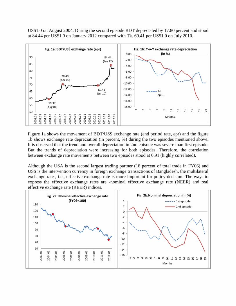
US$1.0 on August 2004. During the second episode BDT depreciated by 17.80 percent and stood
at 84.44 per US$1.0 on January 2012 compared with Tk. 69.41 per US$1.0 on July 2010.
Figure 1a shows the movement of BDT/US$ exchange rate (end period rate, epr) and the figure
1b shows exchange rate depreciation (in percent, %) during the two episodes mentioned above.
It is observed that the trend and overall depreciation in 2nd episode was severe than first episode.
But the trends of depreciation were increasing for both episodes. Therefore, the correlation
between exchange rate movements between two episodes stood at 0.91 (highly correlated).
Although the USA is the second largest trading partner (18 percent of total trade in FY06) and
US$ is the intervention currency in foreign exchange transactions of Bangladesh, the multilateral
exchange rate , i.e., effective exchange rate is more important for policy decision. The ways to
express the effective exchange rates are -nominal effective exchange rate (NEER) and real
effective exchange rate (REER) indices.
59.37 (Aug 04)
70.40 (Apr 06)
69.41 (Jul 10)
84.44 (Jan 12)
50
55
60
65
70
75
80
85
90
20
03.0
1
20
03.0
8
20
04.0
3
20
04.1
0
20
05.0
5
20
05.1
2
20
06.0
7
20
07.0
2
20
07.0
9
20
08.0
4
20
08.1
1
20
09.0
6
20
10.0
1
20
10.0
8
20
11.0
3
20
11.1
0
20
12.0
5
Fig. 1a: BDT/US$ exchange rate (epr)
-18.00
-16.00
-14.00
-12.00
-10.00
-8.00
-6.00
-4.00
-2.00
0.00
1 3 5 7 9
11
13
15
17
19
21
Months
Fig. 1b: Y-o-Y exchange rate depreciation (in %)
1stepi…
60
70
80
90
100
110
120
130
20
03.0
1
20
04.0
1
20
05.0
1
20
06.0
1
20
07.0
1
20
08.0
1
20
09.0
1
20
10.0
1
20
11.0
1
20
12.0
1
Fig. 2a: Nominal effective exchange rate (FY06=100)
-16
-14
-12
-10
-8
-6
-4
-2
0
2
4
1 2 3 4 5 6 7 8 9
10
11
12
13
14
15
16
17
18
19
Months
Fig. 2b:Nominal depreciation (in %)
1st episode
2nd episode

From figure 2a and 2b, it is observed that BDT sharply depreciated in nominal term against its
major trading currencies during the first episode. The depreciation would have been more severe
in the second episode except for the months of September-October, 2009. From figure 3a and 3b,
it is also observed that BDT depreciated in real term in the first episode except for the months of
November-December, 2005 and February 2006. It also depreciated severely in the second
episode except for the months of July-December, 2010, January 2011 and September 2011.
III. Plausible reasons for exchange rate depreciations
Under a floating regime, exchange rate movements depend on the demand and supply of foreign
currency which are determined by the foreign exchange rate as well as money market variables.
Some important variables are discussed below in order to explain the possible reasons for the
sharp depreciation of BDT during the two episodes mentioned above.
(a) Movement of net exports: Net exports in Bangladesh are always negative since its
independence due to merchandise trade account imbalance. The size of the external trade
account deficit becomes smaller or larger at different time periods. The vulnerability of the
net export situation resulted mainly due to inelastic import demand of Bangladesh. About
eighty percent of Bangladesh exports are on account of woven garments and knitwear, which
in-elastically depend on the import of raw materials. The other important import items
namely consumer goods (basically food), machinery and petroleum products are also
inelastic in nature. An increase in net exports increases the demand for foreign exchange and
trends to put pressures on the BDT exchange rate against partners' currencies. From figure 4,
it is observed that net exports of Bangladesh had increased sharply during both the 1st and
2nd episodes. From figure 5, it is apparent that import demands for consumer goods as well
as for petrol and petroleum product were responsible for the higher import demand during the
two episodes under review. It is observed that during the first episode import demand for
petrol and petroleum products was greater than the demand for consumer goods, but during
the second episode demand for consumer goods was much higher than its levels in normal
85
90
95
100
105
110
115
1202
003
.01
20
03.0
9
20
04.0
5
20
05.0
1
20
05.0
9
20
06.0
5
20
07.0
1
20
07.0
9
20
08.0
5
20
09.0
1
20
09.0
9
20
10.0
5
20
11.0
1
20
11.0
9
20
12.0
5
Fig. 3a: Real effective exchange rate (FY06=100)
-10
-8
-6
-4
-2
0
2
4
6
8
1 2 3 4 5 6 7 8 9
10
11
12
13
14
15
16
17
18
19
Months
Fig. 3b: Real depreciation (in %)
1st episode
2nd episode

times. Demand for consumer goods increased sharply in value terms mainly due to increased
food prices in the world market.
(b) Inward remittance: The flows of inward remittances in Bangladesh have contributed
significantly to the external current account surplus recorded in recent years. It is also a very
important source of foreign exchange from the supply side of the foreign exchange market in
Bangladesh and thus can potentially play an important role in exchange rate determination. In
this context it is noteworthy that the remittance growth, especially during the second episode,
was disappointing (Fig. 6). The average growth of inward remittance during the second
episode was 8.29 percent where the historical average of inward remittance was 18.86
percent (during January 2003-June 2012). The slower growth of inward remittances certainly
exacerbated the recent exchange rate pressure in Bangladesh during the second episode.
-1600
-1400
-1200
-1000
-800
-600
-400
-200
0
200
20
03.0
1
20
03.0
9
20
04.0
5
20
05.0
1
20
05.0
9
20
06.0
5
20
07.0
1
20
07.0
9
20
08.0
5
20
09.0
1
20
09.0
9
20
10.0
5
20
11.0
1
20
11.0
9
20
12.0
5
Fig. 4: Net export (in million US$)
0
100
200
300
400
500
600
700
800
900
1000
20
03.0
1
20
03.0
9
20
04.0
5
20
05.0
1
20
05.0
9
20
06.0
5
20
07.0
1
20
07.0
9
20
08.0
5
20
09.0
1
20
09.0
9
20
10.0
5
20
11.0
1
20
11.0
9
20
12.0
5
Fig. 5: LC opening (in million US$)
Consumer goods
Petrol and petrolium products
-20.00
0.00
20.00
40.00
60.00
80.00
100.00
20
04.0
1
20
04.0
8
20
05.0
3
20
05.1
0
20
06.0
5
20
06.1
2
20
07.0
7
20
08.0
2
20
08.0
9
20
09.0
4
20
09.1
1
20
10.0
6
20
11.0
1
20
11.0
8
20
12.0
3
Fig. 6: Remittanc growth (y-o-y)
-100
0
100
200
300
400
500
20
03.0
1
20
03.0
9
20
04.0
5
20
05.0
1
20
05.0
9
20
06.0
5
20
07.0
1
20
07.0
9
20
08.0
5
20
09.0
1
20
09.0
9
20
10.0
5
20
11.0
1
20
11.0
9
20
12.0
5
Fig. 7: Foreign direct investment (in million US$)

(c) FDI inflow: The FDI inflow in Bangladesh has generally been very low compared to most
comparator countries in the region. It was even lower during the two episodes under review
compared to the inflow in between the two episodes (Fig. 7). The monthly average (y-o-y)
FDI inflow during the first and second episodes were US$47.0 million and US$62.2 million
respectively whereas it was US$68.8 million during the period in between the two episodes
(May 2006 - June 2010).
(d) Net foreign aid: Bangladesh is still dependent on international foreign aid for financing its development projects and for the stability of the overall balance of payments. By financing imports
associated with development projects and through budget support, foreign aid is also important
for the stability of the foreign exchange market of the country. The level of foreign aid,
especially during the first episode, was very low compared to the historical average (US$
93.3 million, during January 2003 - June 2012). The monthly average of net amounts of
foreign aid during the first and second episodes were US$69.8 million and US$84.21 million
respectively where as it was US$107.1 million during the period in between the two episodes
(Fig. 8).
(e) FX intervention: Although the floating exchange rate regime has been prevailing,
Bangladesh Bank has to intervene sometimes indirectly through selling and buying of foreign
currency in the market to mitigate the undesirable fluctuations in the exchange rate. In this
context, the amounts of net sales during the first and second episodes were US$1135.9
million and US$1680.5 million, respectively. Market interventions works to smooth out
fluctuations due to temporary or short-term liquidity problems and it never works when the
exchange market is fundamentally in disequilibrium. Since the interventions were made
when the exchange market was subjected to some fundamental shifts on the supply and
demand side both working toward larger excess demand for foreign exchange Bangladesh
Bank interventions were not sufficient to stabilize the market (Fig. 9).
-200
-100
0
100
200
300
400
500
600
700
800
20
03.0
1
20
04.0
1
20
05.0
1
20
06.0
1
20
07.0
1
20
08.0
1
20
09.0
1
20
10.0
1
20
11.0
1
20
12.0
1
Fig. 8: Net foreign aid (in million US$)
-1200
-1000
-800
-600
-400
-200
0
200
400
600
20
03.0
1
20
04.0
1
20
05.0
1
20
06.0
1
20
07.0
1
20
08.0
1
20
09.0
1
20
10.0
1
20
11.0
1
20
12.0
1
Fig. 9: Net FX sale (in million US$)

(f) Liquidity movement: Theoretically, exchange rate depreciation is positively related with the
expansion of money supply (liquidity). From figure 10, it is observed that the growth of
broad money during first episode was increasing. For the second episode it may appear that
liquidity was decelerating when the exchange market pressure emerged. However, a closer
look at the monetary/liquidity situation would indicate that in the period immediately
preceding the start of the episode for a significant period during the second episode, liquidity
expansion remained at the very high level of about 22 percent. Therefore, the impact of
nominal shock behind the sharp depreciation can be supported for both the episodes. This
observation is also supported by the movement of excess reserve and call money rate. From
figure 11, it is observed that the movements of the excess reserves were decline during the
both episodes and the call money rates were comparatively high. It may also be observed that
(Fig. 12) the correlations between volatility of call rate and that of exchange rate (0.63 for
first episode and 0.37 for second episode) were not strong.
10
12
14
16
18
20
22
24
262
003
.01
20
03.0
9
20
04.0
5
20
05.0
1
20
05.0
9
20
06.0
5
20
07.0
1
20
07.0
9
20
08.0
5
20
09.0
1
20
09.0
9
20
10.0
5
20
11.0
1
20
11.0
9
20
12.0
5
Fig. 10:Broad money growth (y-o-y)
0
5
10
15
20
25
30
35
40
-20000
0
20000
40000
60000
80000
100000
120000
20
03.0
1
20
04.0
1
20
05.0
1
20
06.0
1
20
07.0
1
20
08.0
1
20
09.0
1
20
10.0
1
20
11.0
1
20
12.0
1
Fig. 11: Excess reserve and call rate
Excess reserves (milliontaka, LHS)Call money rate(percent, RHS)
-10
-5
0
5
10
15
20
25
-10
-5
0
5
10
15
20
25
20
03.0
1
20
04.0
1
20
05.0
1
20
06.0
1
20
07.0
1
20
08.0
1
20
09.0
1
20
10.0
1
20
11.0
1
20
12.0
1
Fig. 12: Volatility as measured by deviation
Volatility of call rate (LHS)
Volatility of exchange rate (RHS)
0
2000
4000
6000
8000
10000
12000
20
03.0
1
20
03.0
9
20
04.0
5
20
05.0
1
20
05.0
9
20
06.0
5
20
07.0
1
20
07.0
9
20
08.0
5
20
09.0
1
20
09.0
9
20
10.0
5
20
11.0
1
20
11.0
9
20
12.0
5
Fig. 13: Movements of FX reserves (in million US$)

(g) Foreign exchange reserves: Due to both domestic and external factors discussed above the
level of foreign exchange reserves was decreasing during both episode, in part because of
market interventions. Bangladesh Bank’s inability to stabilize the exchange rate despite
sizable market interventions and the consequent loss of reserves led to a sharp exchange rate
depreciation pressure in during the two episodes in Bangladesh.
IV. Model based analysis of exchange rate fluctuations
Theoretical background
Following the pioneering work of Blanchard and Quah (1989), there has been a growing body of
literature in which long-run relationships from theory are used to identify structural shocks in an
open economy setting. Clarida and Gali (1994) construct a three variable - relative output,
relative prices, and the real exchange rate - structural VAR and identify three types of
macroeconomic shocks: supply, real demand, and nominal shocks. The contribution of each type
of shock to the variability of each variable is then assessed.
Clarida and Gali (1994) derive a stochastic version of the Obstfeld (1985) open economy macro
model where output is supply determined over the long run. Their representation illustrates how
the Mundell-Fleming-Dornbusch model can provide theoretical foundations for the restrictions
used in their analysis to identify three separate types of “fundamental” shocks in the economy.
The key assumptions of the model include (i) prices and output adjustments are sticky and (ii)
foreign and domestic goods are imperfect substitutes in consumption. Shocks in the model can
be categorized into: (i) real aggregate supply (AS) shocks, which includes all labor market
factors, such as changes in the relative productivity of home to foreign countries, that shift the
aggregate supply curve; (ii) aggregate demand or real good market (IS) shocks, encompassing
exogenous changes to real relative domestic absorption due to shifts in consumption, investment,
government expenditure and home/foreign goods tastes; and (iii) nominal or money market
(LM) shocks, reflecting shifts in both relative money supplies, such as monetary policy shocks
and relative money demands, such as velocity shifts, and effects of financial liberalization.
A positive supply shock, such as a higher productivity growth in the home country, raises the
aggregate supply of domestic goods and the rate of return to capital and, in a traditional Mundell-
Fleming model in which capital is mobile, leads to capital inflows and an appreciation of the
exchange rate on impact (Obstfeld, 1994). Over the long run, domestic output increases to its
higher potential level, domestic price declines, and the real exchange rate depreciates in order to
generate trade surpluses to pay down the accumulated stock of net foreign liabilities. A positive
demand shock increases demand for home goods, pushes up prices of home products and leads to
an appreciation of the real exchange rate and an increase in output in the short run. Over time,
output returns to the long-run trend, but the price level remains higher and the real exchange rate
remains above its trend. A positive nominal shock lowers home interest rates. In the short run,
both the nominal and real exchange rates depreciate, the relative price rises, and the domestic
output increases. Over time, output and the real exchange rate return to their long-run trends. The
long-run relationships described here are used in this paper as restrictions to identify the
fundamental shocks in the model.

Data and Variables Three variables - relative output (y), relative prices (p) and the real exchange rate (q) - have been
included in this study. Monthly data on these variables have been collected for the period from
January 2003 to June 2012. All variables are expressed in natural logarithms. The variables are
relative to the weighted average of same variables in eight largest trading partner countries
because both domestic and external macroeconomic conditions may affect the real exchange
rate. Due to unavailability of quarterly or monthly data on GDP in Bangladesh, in this paper the
index of industrial production (IIP) is used as a proxy of output variable. Hence, the log of
relative real output is measured as the log of IIP of Bangladesh minus the log of trade weighted
IIP of trading partner countries; the relative price level (CPI) has been measured similarly. Data
on these variables related to Bangladesh have been collected from various publications of
Bangladesh Bank and Bangladesh Bureau of Statistics (BBS). On the other hand, data related to
trading partner countries have been collected from the CD-ROM of International Financial
Statistics (IFS).

Model The empirical model contains a three-variable structural VAR (∆y, ∆q, ∆p) and its identification
restriction. The observed variations of economic variables are governed by three mutually
orthogonal disturbances: supply shocks, demand shocks and monetary shocks. Formally, we
want to transform the reduced form VAR to the structural model:
( ) (1)
where
, ( )
( ) ( ) ( )
( ) ( ) ( )
( ) ( ) ( ) ,
(2)
In equation (2), Cij(L) is the polynomial of lag operator L, and ,
and are sequences of
supply, demand and monetary shocks respectively. The orthogonality assumption implies
E . Furthermore, following Clarida and Gali (1994), the restriction that neither
monetary shocks nor demand shocks
influence relative output levels in the long run
requires that
( ) ( ) (3)
Similarly, the restriction that monetary shocks do not influence the real exchange rate in the
long run implies that
( ) (4)
Estimation Procedure First, the reduced form VAR will be estimated by ordinary least square regression (OLS).
Second, from the estimated reduced form VAR and long-run restriction denoted in equations (3)
and (4), three orthogonal shocks can be disentangled, yielding the estimated coefficients {Cij:i,j=
1,2,3} in equation (2). Finally, the paper will employ impulse response and variance
decompositions, which help us to investigate the direction and the sources of real exchange rate
fluctuations.
Estimation Results This section examines the time-series properties of the variables in the analysis. As we see in
Figure 14, three variables included in this study are most likely to have unit roots. Regression of
non-stationary variables may leads to a spurious result. Formal stationary tests are conducted and
the results from the Augmented Dickey Fuller unit root tests are reported in Table 1. The null
hypothesis of a unit root cannot be rejected for the levels of all three variables at conventional
level of significance, while the first differences are confirmed to be stationary at 1 percent level
of significance.

Fig. 14: Movements of variables
Table 1: Augmented Dickey-Fuller Test for Stationarity
Variables In Level In first difference
t-statistic t-statistic
Relative output 0.41 -10.16*
REER -2.34 -9.81*
Relative Price level 1.70 -7.70*
Note: * test statistic significant at 1 percent level of significance.
Using the Akaike Information Criterion (AIC), we find that the Vector Auto Regressive (VAR)
model is the most appropriate for the system. In order to examine the sources of fluctuation,
computed impulse response functions (IRFs) and variance decompositions (VDCs) of these three
variables have been used. Since the nominal exchange rate is of central interest to us, below we
also present the impulse response analysis for this variable2.
Figure 15 displays the impulse response functions of relative output, real exchange rate, relative
price level and nominal exchange rate to one standard deviation structural shocks. Since the
variables were entered in first differences in the VAR, the resulting impulse responses were
cumulated in order to obtain the impulse responses of level of each of the variable to the
structural shocks in the model. These impulse response functions are in line with the theoretical
priors discussed above. Figure 15 shows that a positive supply shock leads to an increase in
output; however, it declines to a lesser rise over the long run. The increase in relative output in
2 Even though this variable does not enter our empirical model directly, it can be constructed from the relative price
variable and the real exchange rate variable.
0.6
0.8
1.0
1.2
1.4
1.6
1.8
2.0
90
95
100
105
110
115
2003 2004 2005 2006 2007 2008 2009 2010 2011 2012
REER
Relative Price
Relative Output

Bangladesh is accompanied by a relative decline in the price level in Bangladesh. Since it is a
key characteristic of a supply disturbance to drive output and prices in opposite directions, the
responses shown in the figure are consistent with the predictions of our theoretical model. The
real exchange rate initially appreciates slightly in response to the supply disturbance, but then a
pronounced and persistent depreciation sets in, which is the long-run response predicted by
Clarida and Gali’s model. To quantify the impulse response of nominal exchange rate we deduct
the response of relative price from the response of real exchange rate. The figure shows that in
response to supply shock, nominal exchange rate appreciates slightly in the long run and the
response seems to be very weak.
In the case of real demand shock, there is an increase in output, an increase in the price level, and
an appreciation of the real exchange rate. Both responses are predicted by our theoretical model.
The nominal exchange rate also appreciates. In the long run, the output response is restricted to
zero. The price and the exchange rate responses, on the other hand, turn out to be very persistent.
In the case of nominal shock, the output response lasts for a few months and is accompanied by a
depreciation of the nominal and real exchange rate. In the long-run, both the output and the real
exchange rate responses are restricted to zero. But the nominal disturbance is followed by a
persistent increase in the price level, and, consequently, in the nominal exchange rate. It is
noteworthy that the nominal exchange rate overshoots its long-run level considerably, which is
consistent with the predictions of the familiar Dornbusch (1976) model.
Fig. 15: Accumulated Impulse Response Function
Impulse response of relative output Impulse response of real exchange rate
Impulse response of relative price Impulse response of nominal exchange rate
-.02
-.01
.00
.01
.02
.03
.04
.05
.06
2 4 6 8 10 12 14 16 18 20 22 24 26 28 30
Supply Shock Demand Shock Nominal Shock
-.010
-.005
.000
.005
.010
.015
.020
.025
2 4 6 8 10 12 14 16 18 20 22 24 26 28 30
Supply Shock Demand Shock Nominal Shock
-.006
-.004
-.002
.000
.002
.004
.006
.008
.010
2 4 6 8 10 12 14 16 18 20 22 24 26 28 30
Supply Shock Demand Shock Nominal Shock
-.010
-.005
.000
.005
.010
.015
.020
2 4 6 8 10 12 14 16 18 20 22 24 26 28 30
Supply Shock Demand Shock Nominal Skock

While impulse responses are useful in assessing the signs and magnitudes of responses to
specific shocks, the forecast error variance decomposition analysis provides an important insight
into the relative importance of each shock at different forecast horizons to the structural
disturbances in our model. Since this paper focuses on the nominal exchange rate, we report here
the variance decomposition only for the nominal exchange rate, which has been produced from
the variance decomposition of real exchange rate and relative price. Table 2 presents the share of
the forecast error variance of nominal exchange rate at different forecast horizon that can be
attributed to each type of shocks in the model.
Table 2 shows that the main cause of the unexpected changes in the nominal exchange rate is
demand shock. Demand shock accounts for almost half of the short-run variability in the nominal
exchange rate. At the one-year horizon, nominal disturbances still account for about 60 percent
of the variance decomposition, but at the two-year horizon this share has declined to about one-
third. It decreases slightly to 46.56 percent at six month forecast horizon and it remained
persistent for longer forecast horizon. While nominal shocks are the second largest source of the
variability in nominal exchange rate which accounts for one-third of the unexpected fluctuations
of the nominal exchange rate and it remains persistent in the longer forecast horizon. Initially
supply shocks account for only 17.53 percent of the variability in nominal exchange rate. It
increases to 20.44 percent at eight month forecast horizon and remains persistent thereafter.
Table 2: Forecast Error Variance Decomposition of Nominal Exchange Rate
Forecast horizon Supply shock Demand shock Nominal shock
1 17.52 48.10 34.38
2 17.68 47.79 34.53
3 18.27 47.92 33.81
4 19.35 47.99 32.66
5 19.73 47.33 32.94
6 19.94 46.56 33.49
7 20.27 46.60 33.13
8 20.44 46.57 32.99
9 20.38 46.60 33.03
10 20.55 46.42 33.03
11 20.56 46.42 33.02
12 20.56 46.40 33.04
In this paper our main objective is to identify the sources of volatility of nominal exchange rate
with special attention to two episodes (Episode 1: August 2004 - April 2006 and Episode 2: July
2010 - January 2012) of high depreciation pressure on nominal exchange rate in Bangladesh.
This purpose may be better served by historical decomposition of the nominal exchange rate.
Using the estimated VAR, a historical decomposition can be derived to examine whether or not
the supply, demand, and nominal shocks that have been identified can plausibly explain the time
path followed by the nominal exchange rate of Bangladesh during the two episodes mentioned
earlier.

Figure 16: Historical Decomposition of Nominal Exchange Rate During the Two Episodes
Episode 1 Episode 2
Figure 16 plots the unconditional forecast error for the nominal exchange rate and shows the
decomposition of this forecast error into the components that can be attributed to supply, real
demand, and nominal shocks. The blue line in each graph of two panels (for two episodes) is the
total forecast error, which depicts the difference between the actual (log level of the) nominal
-.06
-.05
-.04
-.03
-.02
-.01
.00
.01
.02
.03
III IV I II III IV I II
2004 2005 2006
Movements in Nominal Exchange Rate Minus Trend
Due to Supply Shock
-.06
-.04
-.02
.00
.02
.04
III IV I II III IV I
2010 2011
Movements in Nominal Exchange Rate Minus Trend
Due to Supply Shock
-.06
-.05
-.04
-.03
-.02
-.01
.00
.01
.02
.03
III IV I II III IV I II
2004 2005 2006
Movements in Nominal Exchange Rate Minus Trend
Due to Demand Shock
-.06
-.04
-.02
.00
.02
.04
III IV I II III IV I
2010 2011
Movements in Nominal Exchange Rate Minus Trend
Due to Demand Shock
-.06
-.05
-.04
-.03
-.02
-.01
.00
.01
.02
.03
III IV I II III IV I II
2004 2005 2006
Movements in Nominal Exchange rate Minus Trend
Due to Nominal Shocks
-.06
-.04
-.02
.00
.02
.04
III IV I II III IV I
2010 2011
Movements in Nominal Exchange Rate Minus Trend
Duen to Nominal Shock

exchange rate and the level that would have been forecast from the VAR. In other words, the
blue line reflects the cumulative impact of the three types of structural shocks on the nominal
exchange rate. The red line in each panel plots the contribution of each type of shocks to the total
forecast error, or the forecast error that would have resulted if only one particular source of
shocks had hit the variable. As shown in the figure, unexpected movements in the nominal
exchange rate have been driven mainly by demand shocks.
Government expenditure which is a component of aggregate demand expands very largely
during both episodes (Figure 17). The average quarterly growth of government expenditure stood
at 19.37 percent and 40.51 percent during the 1st and 2
nd episode respectively, whereas the
average growth between two episodes was 15.79 percent. The growth of other components of
aggregate demand except net exports (exports minus imports) also increases largely during the
two episodes compared to pre-episodes periods (Figure 18a and Figure 18b).
-40
-20
0
20
40
60
80
0
100
200
300
400
500
600
20
03
.03
20
03
.08
20
04
.01
20
04
.06
20
04
.11
20
05
.04
20
05
.09
20
06
.02
20
06
.07
20
06
.12
20
07
.05
20
07
.10
20
08
.03
20
08
.08
20
09
.01
20
09
.06
20
09
.11
20
10
.04
20
10
.09
20
11
.02
20
11
.07
20
11
.12
20
12
.05
Fig. 17: Trend of government expenditure
Govt. expenditure in billion taka (LHS)
Quarterly growth of govt. expenditure (RHS)
0
2
4
6
8
10
12
14
16
18
0
1000
2000
3000
4000
5000
6000
7000
8000
20
02
20
03
20
04
20
05
20
06
20
07
20
08
20
09
20
10
20
11
20
12
Fig. 18a: Consumption expenditure
Consumption (in billion taka,LHS)Consumption growth (RHS)
0.00
2.00
4.00
6.00
8.00
10.00
12.00
14.00
16.00
18.00
20.00
0
500
1000
1500
2000
2500
20
02
20
03
20
04
20
05
20
06
20
07
20
08
20
09
20
10
20
11
20
12
Fig. 18b. Investment expenditure
Investment (in billiontaka, LHS)Investment growth(RHS)

The growths of consumption during 1st and 2
nd episodes were 11.24 percent and 15.31 percent
respectively, whereas the growths were 9.47 percent and 13.74 percent during pre-episodes
respectively. The growths of investment during 1st and 2
nd episodes were 13.19 percent and
17.19 percent respectively, while the growths were 12.47 percent and 13.41 percent during pre-
episodes respectively. As a result, the nominal GDP growths during 1st and 2
nd episodes were
11.74 percent and 14.78 percent respectively, whereas the growths were 10.40 percent and 13.69
percent during pre-episodes respectively.
V. Concluding remarks
In order to find out the recent exchange rate fluctuations in Bangladesh, this paper has discussed
all relevant variables of foreign exchange market and money market using graphical as well as
econometric technique. This paper also tries to find out the reasons behind the exchange rate
fluctuations on historical as well as episode basis. It is observed that demand shocks especially
created from external sector are responsible for sharp depreciation of BDT exchange rate during
the two episodes. As per econometric analysis supply shocks are also important (but less than
demand shock) for exchange rate fluctuation. The nominal shock, i.e., the money supply shock is
ignored in the overall analysis.
References
Bhundia, A. & Gottschalk, J. (2003). Sources of Nominal Exchange Rate Fluctuations in South
Africa. IMF Working paper No. WP/03/252.
Blanchard, O. & Quah, D. (1989). The Dynamic Effects of Aggregate Supply and Demand
Disturbances. American Economic Review, 79(4): 655–673.
Chen, S. (2004). Real Exchange Rate Fluctuations and Monetary Shocks: A Revisit.
International Journal of Finance and Economics, 9:25-32.
Clarida, R. & Gali, J. (1994). Sources of Real Exchange Rate Fluctuations: How Important are
Nominal Shocks? NBER Working paper no. 4658.
Dornbusch, R. (1976). Expectations and Exchange rate dynamics. Journal of Political Economy,
84:1161–76.
Inoue, T. & Hamori, S. (2009). What Explains Real and Nominal Exchange Rate Fluctuations?
Evidence from SVAR analysis for India. Discussion paper no. 216, Institute of Developing
Economics, Japan.
Obstfeld, M. & Rogoff, K. (1995). Exchange Rate Dynamics Redux. Journal of Political
Economy, 102: 624–660.
Rahman, M. H. & Barua, S. (2006). Recent experiences in the foreign exchange and money
markets, Policy Note Series: PN 0703, Policy Anlysis Unit (PAU), Bangladesh Bank.
Wang, T. (2004). China: Sources of Real Exchange Rate Fluctuations. IMF Working Paper No.
WP/04/18.