When and Why do Plants Comply? Paper Mills in the 1980s

Wayne B. Gray and Ronald J. Shadbegian

Working Paper Series

Working Paper # 04-07 June, 2004

U.S. Environmental Protection Agency National Center for Environmental Economics 1200 Pennsylvania Avenue, NW (MC 1809) Washington, DC 20460 http://www.epa.gov/economics

When and Why do Plants Comply? Paper Mills in the 1980s

Wayne B. Gray and Ronald J. Shadbegian

Correspondence: Ronald J. Shadbegian UMass Dartmouth

Department of Economics North Dartmouth, MA 02747

email: rshadbegian@umassd.edu 508-999-8337

and U.S. Environmental Protection Agency

National Center for Environmental Economics email: shadbegian.ron@epa.gov

NCEE Working Paper Series

Working Paper # 04-07 June, 2004

DISCLAIMER The views expressed in this paper are those of the author(s) and do not necessarily represent those of the U.S. Environmental Protection Agency. In addition, although the research described in this paper may have been funded entirely or in part by the U.S. Environmental Protection Agency, it has not been subjected to the Agency's required peer and policy review. No official Agency endorsement should be inferred.

When and Why do Plants Comply? Paper Mills in the 1980s

Wayne B. Gray Clark University and NBER

Ronald J. Shadbegian University of Massachusetts at Dartmouth

U.S. EPA National Center for Environmental Economics

Subject Area: Air Pollution, Enforcement Issues, and Environmental Policy Key Words : 1) Air Pollution Regulation; 2) Compliance; 3) Enforcement; 4) Inspections

Financial support for the research from the National Science Foundation (grant # SBR­9809204) and the Environmental Protection Agency (grants #R-826155-01-0 and #R­828824-01-0) is gratefully acknowledged, as is access to Census data at the Boston Research Data Center. Valuable comments were received from Alex Pfaff, Suzi Kerr, Amanda Lee, and Maureen Cropper, as well as seminar participants in the AERE Summer Workshop, the NBER Summer Institute, Lehigh University, Center for Economic Studies, the University of California-Berkeley, and a 2003 AERE-ASSA session. We are grateful to the many people in the paper industry who were willing to share their knowledge of the industry with us. Capable research assistance was provided by Bansari Saha, Aleksandra Simic, Nadezhda Baryshnikova and Melanie Lajoie. The opinions and conclusions expressed are those of the authors and not the Census Bureau, EPA, or NSF. All papers using Census data are screened to ensure that they do not disclose confidential information. Any remaining errors or omissions are the authors'.

Abstract

This paper examines differences in compliance with air pollution regulation for U.S. pulp and paper mills. Our analysis is based on confidential, plant-level Census data from the Longitudinal Research Database for 116 pulp and paper mills, covering the 1979-1990 period. The LRD provides us with data on shipments, investment, productivity, age, and production technology. We also have plant-level pollution abatement expenditures from the Pollution Abatement Costs and Expenditures (PACE) survey. Using ownership data, we link in firm-level financial data taken from Compustat, identifying firm size and profitability. Finally, we use several regulatory data sets. From EPA, the Compliance Data System provides measures of air pollution enforcement activity and compliance status during the period, while the Permit Compliance System and the Toxic Release Inventory provide information on other pollution media. OSHA's Integrated Management Information System provides data on OSHA enforcement and compliance.

We find significant effects of some plant characteristics on compliance rates: plants which include a pulping process, which are older, and which are larger are all less likely to be in compliance. Compliance also seems to be correlated across media: plants violating water pollution or OSHA regulations are more likely to violate air pollution regulations. Firm-level characteristics are not significant determinants of compliance rates.

Once we control for the endogeneity of regulatory enforcement, we find the expected positive relationship between enforcement and compliance. We also find some differences across plants and firms in their responsiveness to enforcement. Pulp mills, already less likely to be in compliance, are also less sensitive to inspections. Some firm characteristics also matter here: plants owned by larger firms, whether measured in terms of their employment or by the number of other paper mills they own, are less sensitive to inspections and more sensitive to other enforcement actions, consistent with our expectations and with other researcher’s results.

1. Introduction

In most economic models of government regulation, a regulatory agency establishes

standards with which regulated firms are required to comply. Compliance is usually

accomplished by having inspectors visit plants to identify violations and to impose penalties on

violators. Becker (1968) demonstrated that if both the probability of being caught and the

penalty for violations are high (relative to the costs of compliance), we would expect profit-

maximizing firms to optimally choose compliance. However, for many regulatory agencies, the

number of inspectors is small relative to the regulated population and the penalties are limited, so

there seems to be a limited incentive for compliance - yet most firms still seem to comply.

This puzzle of 'excessive' compliance has led to several strands of literature. Outside

economics, researchers have emphasized the importance of social norms and a corporate

culture that encourages compliance, and have conducted interviews to identify how corporate

decisions are affected by pressures from both regulatory agencies and the general public.

Within economics, a model by Harrington (1988) shows that in a repeated game, a regulator

could substantially increase the expected long-run penalty for non-compliance by creating two

classes of regulated firms - cooperative and non-cooperative. The cooperative firms are

assumed to behave well and to be inspected only rarely. The non-cooperative firms would face

much heavier enforcement. Since facing enforcement is costly, firms would be anxious to be

placed in the cooperative group initially, and therefore would invest more in compliance at the

start of the game, than would be predicted from the expected penalty in a one-period model.

On the empirical side, there have been several studies on the effectiveness of OSHA

and EPA enforcement, using a variety of estimation techniques. These include studies of

1

environmental enforcement at steel mills for air pollution (Gray and Deily 1996); at paper mills

for air pollution (Nadeau 1997) and water pollution [Magat and Viscusi (1990), Laplante and

Rilstone (1996), and Helland (1998)]; and of OSHA regulation at manufacturing plants (Gray

and Jones(1991), and Gray and Scholz(1993)). These studies generally find that enforcement

has some effect on compliance, or the goals of compliance (reduced emissions or injuries).

Since enforcement and compliance tend to be defined at the plant level, most of these studies do

not incorporate firm-level variables. However, Helland finds that more profitable firms have

fewer violations, and Gray and Deily find that compliance status is correlated across plants

owned by the same firm, though they find insignificant effects of firm size and profitability on

compliance. Gray (2000) finds little effect of corporate ownership change or restructuring on

compliance and enforcement.

In this paper we use a sample of U.S. pulp and paper mills to examine differences in

plant-level compliance with air pollution regulations. In particular, we test a variety of plant- and

firm-specific characteristics, to see which plants are more likely to comply with regulation. We

also compare the plant's air pollution compliance with its performance in other dimensions

(water pollution, toxic chemicals, and worker health and safety). Finally, we test how effective

regulatory enforcement is at inducing compliance, and whether plants differ in their sensitivity to

enforcement activity.

We use confidential, plant-level Census data from the Longitudinal Research Database

for 116 pulp and paper mills, covering the 1979-1990 period. The LRD provides us with data

on each plant's shipments, investment, productivity, age, and production technology. We also

have plant-level pollution abatement expenditures from the Pollution Abatement Costs and

Expenditures (PACE) survey. We link in ownership information, based on the Lockwood

2

Directory, which allows us to identify the number of paper mills owned by the firm, and also link

in firm-level financial data taken from Compustat, identifying firm size and profitability. Finally,

we add compliance and enforcement information from several regulatory data sets, although our

focus is on the EPA's Compliance Data System, which provides measures of air pollution

enforcement activity and compliance status during the period.

We use a logit model of compliance with air pollution regulation: compliance depends

on regulatory activity directed towards the plant, as well as various plant and firm

characteristics. Regulatory activity is endogenous - regulators target enforcement activity

towards plants that are out of compliance – so a simple correlation between enforcement and

compliance would be negative, indicating (naively) that enforcement decreases compliance. To

address this targeting issue, we try two alternative ways of measuring enforcement. First, we try

using lagged enforcement as an explanatory variable, in principle purging the equations of any

contemporaneous endogeneity. Second, we try predicting enforcement from a tobit model on a

set of variables which are clearly exogenous to the plant's compliance decision (state political

support for environmental regulation and year and state dummies). We then use this predicted

value in a second-stage compliance equation. Models using lagged regulatory activity continue

to find a negative 'impact' of enforcement on compliance (which we attribute to remaining

endogeneity), while models using predicted activity yield positive coefficients, with regulatory

activity increasing compliance.

We find significant effects of plant characteristics on compliance rates: plants which

include a pulping process, plants which are older, and plants which are larger are all less likely

to be in compliance. In contrast, firm-level characteristics are not significant determinants of

plant-level compliance rates. Plants violating other regulations (water pollution or OSHA

3

regulations) are more likely to violate air pollution regulations.

We also find differences across plants in their responsiveness to enforcement. Pulp

mills, already less likely to be in compliance, are also less sensitive to inspections. Finally, firm

characteristics do seem to matter for a plant’s inspection sensitivity (though they did not for the

overall compliance rate). Plants owned by larger firms, whether measured in terms of firm

employment or the number of paper mills owned by the firm, are less sensitive to inspections

and more sensitive to other enforcement actions than plants owned by smaller firms.

Section 2 provides some background on environmental regulation and compliance

issues in the paper industry. Section 3 describes a simple model of the compliance decision

faced by a plant. Section 4 describes the data used in the analysis, Section 5 describes some

econometric issues with the analysis, Section 6 presents the results, and Section 7 contains the

concluding comments.

2. Paper Industry Background

Environmental regulations have grown substantially in stringency and enforcement

activity over the past 30 years. In the late 1960s the rules were primarily written at the state

level, and there was little enforcement. Since the early 1970s, the Environmental Protection

Agency has taken the lead in developing stricter regulations, and encouraging greater

enforcement (much of which is still done by state agencies, following federal guidelines). This

expanded regulation has imposed sizable costs on traditional 'smokestack' industries, with the

pulp and paper industry being one of the most affected, given its substantial generation of air and

water pollution.

Plants within the pulp and paper industry can face very different impacts of regulation,

4

depending in part on the technology being used, the plant's age, and the regulatory effort

directed towards the plant. The biggest determinant of regulatory impact is whether or not the

plant contains a pulping process. Pulp mills start with raw wood (chips or entire trees) and

break them down into wood fiber, which are then used to make paper. A number of pulping

techniques are currently in use in the U.S. The most common one is kraft pulping, which

separates the wood into fibers using chemicals. Many plants also use mechanical pulping (giant

grinders separating out the fibers), while others use a combination of heat, other chemicals, and

mechanical methods. After the fibers are separated out, they may be bleached, and mixed with

water to form a slurry. After pulping, a residue remains which was historically dumped into

rivers (hence water pollution), but now must be treated. The process also takes a great deal of

energy, so most pulp mills have their own power plant, and therefore are significant sources of

air pollution. Pulping processes involve hazardous chemicals, raising issues of toxic releases.

The paper-making process is much less pollution intensive than pulping. Non-pulping

mills either buy pulp from other mills, or recycle wastepaper. During paper-making, the slurry

(more than 90% water at the start) is set on a rapidly-moving wire mesh which proceeds

through a series of dryers in order to extract the water, thereby producing a continuous sheet of

paper. Some energy is required, especially in the form of steam for the dryers, which can raise

air pollution concerns if the mill generates its own power. There is also some residual water

pollution as the paper fibers are dried. Still, these pollution problems are much smaller than

those raised in the pulping process.

Over the past 30 years, pollution from the paper industry has been greatly reduced, with

the installation of secondary wastewater treatment, electrostatic precipitators, and scrubbers. In

addition to these end-of-pipe controls, some mills have changed their production process, more

5

closely tracking material flows to reduce emissions. In general, these changes have been much

easier to make at newer plants, which were designed at least in part with pollution controls in

mind (some old pulp mills were deliberately built on top of the river, so that any spills or leaks

could flow through holes in the floor for 'easy disposal'). These rigidities can be partially or

completely offset by the tendency for regulations to include grandfather clauses, exempting

existing plants from most stringent air pollution regulations.

3. Compliance and Enforcement Decisions

An individual paper mill faces costs and benefits from complying with environmental

regulation, which may depend on characteristics of the plant itself, the firm which owns the plant,

and the activity of environmental regulators. Given these constraints, the firm operating the mill

is presumed to maximize its profits, choosing to comply if the benefits (lower penalties, better

public image) outweigh the costs (investment in new pollution control equipment, managerial

attention). Regulators, in turn, allocate their activity to maximize some objective function

(political support, compliance levels, economic efficiency), taking into account the reactions of

firms to that activity.

The objective function for mill i owned by firm j at time t includes the usual revenues and

costs of production, but these are extended to include the penalties associated with being found

in violation (Penalty), the probability of being found in violation (VProb), and the costs of

coming into compliance (CompCost):

(1) Profitijt(Comply) = Pijt*Qijt – Costijt – Penaltyijt*VProbijt(Comply) –

CompCostijt(Comply)

Plants can vary their level of compliance (Comply) to maximize their profits (this assumes that

6

the underlying compliance decision is in fact continuous, although we only observe a 0-1

compliance status in our data. Assuming that the benefits and costs of compliance are captured

in the last two terms of equation (1), the plant will set its marginal cost of compliance equal to

the marginal benefit from compliance, measured here in terms of reductions in expected

penalties.

(2) d(-Penaltyijt*VProbijt)/dComply = d(CompCostijt)/dComply

This implicitly determines an optimal level of compliance, Comply*.

The benefits to the firm from increasing compliance come in terms of reducing the

probability of being found in violation of pollution regulations, thus reducing the expected

penalties for violations. These penalties are usually associated with regulators in terms of legal

sanctions and monetary fines, but could also be 'imposed' by customers boycotting the firm's

products in the future. In some circumstances customers might also be willing to pay more for

products that have been certified to have especially environmentally friendly production

processes, although this is currently more common in Europe than in the U.S. If we make the

usual assumption that the firm is risk-neutral, the expected benefits of compliance should be

linear in the probability of being in non-compliance, so the marginal benefit to the plant from

increasing its probability of compliance would be constant. Because of the difficulties

associated with ensuring 100% compliance, we expect a rising marginal cost curve. Rising

marginal costs along with constant marginal benefits should lead to an interior Comply* solution,

equating the marginal costs and marginal benefits of compliance to the firm.

We focus on differences in compliance behavior across different mills, based on plant

and firm characteristics. As mentioned earlier, there are likely to be substantial differences in

pollution problems across different types of paper mills. We expect to see differences in

7

compliance behavior being related to the production technology at the plant (especially the use

of pulping) and related to the plant's age. There may also be economies of scale in complying

with regulations, so larger plants might find it easier to comply with a given level of stringency.

However, some of these plant characteristics on compliance could go either way: older plants

might find it harder to comply with a given standard, but they could be subject to less strict

standards due to grandfathering. Larger plants might enjoy economies of scale, but could also

have more places that something could go wrong, raising their probability of non-compliance.

Compliance behavior may also depend on characteristics of the firm which owns the mill

(e.g. the financial situation of the firm may matter). Pollution abatement can involve sizable

capital expenditures, which may be easier for profitable firms to fund - either through retained

earnings or through borrowing in capital markets. A firm in financial distress may not feel the full

threat of potential fines in an expected value sense, if they would just go bankrupt if they

happened to be caught. Firms with reputational investments in the product market may face an

additional incentive not to be caught violating environmental rules, if their customers would react

badly to the news.

Firms might also differ in the quality of the environmental support that they offer their

plants. A large firm, or one specializing in the paper industry, is likely to have economies of

scale in learning about what regulations require, and may be in a better position to lobby

regulators on behalf of their plants. We cannot measure the strength of a company's

environmental program, but may observe a correlation in compliance behavior across plants

owned by the same firm. We may also see some effect of the firm size, either in absolute

magnitude or in terms of the number of mills they operate.

The regulatory activity faced by a plant is also expected to affect its compliance

8

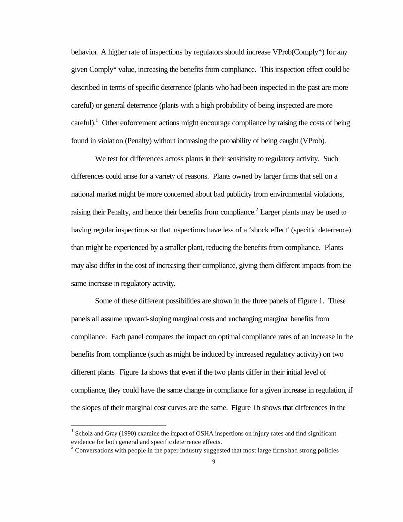
behavior. A higher rate of inspections by regulators should increase VProb(Comply*) for any

given Comply* value, increasing the benefits from compliance. This inspection effect could be

described in terms of specific deterrence (plants who had been inspected in the past are more

careful) or general deterrence (plants with a high probability of being inspected are more

careful).1 Other enforcement actions might encourage compliance by raising the costs of being

found in violation (Penalty) without increasing the probability of being caught (VProb).

We test for differences across plants in their sensitivity to regulatory activity. Such

differences could arise for a variety of reasons. Plants owned by larger firms that sell on a

national market might be more concerned about bad publicity from environmental violations,

raising their Penalty, and hence their benefits from compliance.2 Larger plants may be used to

having regular inspections so that inspections have less of a ‘shock effect’ (specific deterrence)

than might be experienced by a smaller plant, reducing the benefits from compliance. Plants

may also differ in the cost of increasing their compliance, giving them different impacts from the

same increase in regulatory activity.

Some of these different possibilities are shown in the three panels of Figure 1. These

panels all assume upward-sloping marginal costs and unchanging marginal benefits from

compliance. Each panel compares the impact on optimal compliance rates of an increase in the

benefits from compliance (such as might be induced by increased regulatory activity) on two

different plants. Figure 1a shows that even if the two plants differ in their initial level of

compliance, they could have the same change in compliance for a given increase in regulation, if

the slopes of their marginal cost curves are the same. Figure 1b shows that differences in the

1 Scholz and Gray (1990) examine the impact of OSHA inspections on injury rates and find significant evidence for both general and specific deterrence effects.2 Conversations with people in the paper industry suggested that most large firms had strong policies

9

slopes of the marginal cost of compliance can result in very different impacts from the same

increase in regulation – here the plant with high and steep compliance costs has both lower initial

compliance and a smaller impact from the increased regulation. Finally, Figure 1c shows that

plants with the same marginal cost of compliance can respond differently if the same increase in

regulation has different marginal benefits for them, as might happen if the larger firm felt a greater

desire to avoid adverse publicity (MB1’).

In sum, a plant's compliance decision depends on its age and production technology, its

firm size and profitability, and the regulatory activity directed towards it, with the possibility of

some differences across plants in their sensitivity to that regulatory activity. We estimate a

model of compliance behavior as follows:

(3) Comply*ijt = f(REGSijt, Xi, Xj, Xijt*REGSijt, OComplyijt, YEARt).

COMPLY is the plant's observed compliance status with air pollution regulations. REGS is the

regulatory activity faced by the plant, which could be either inspections or other enforcement

actions. This activity could affect either the probability of being caught in violation or the

negative consequences associated with being caught. The model includes characteristics of the

plant (Xi) and firm (Xj), either of which could be interacted with enforcement activity to test for

differences in the responsiveness of plants and firms to enforcement. The plant’s compliance

status with other regulatory areas is measured by OComply. Finally, year dummies (YEARt)

allow for changes in enforcement, or its definition, over time.

Now consider the regulator's decision about how to allocate its regulatory activity. If

enforcement were costless, regulators could use 'infinite' enforcement, catching all violators, in

which case setting a fine equal to the environmental damages from pollution would be optimal.

encouraging 100% compliance as much as possible, perhaps due to these concerns with adverse publicity. 10

Becker (1968) notes that in a world with costly and uncertain enforcement, higher penalties

might be substituted for some of the enforcement effort, to raise the expected penalty for

violations. In fact, given limitations on the size of penalties under existing regulations, and the

high costs of controlling some pollutants, it seems puzzling why any firms would comply with

regulation. However, Harrington (1988) showed that a regulator could substantially raise the

effectiveness of enforcement, by making future enforcement conditional on past compliance. In

this model, non-compliance today not only raises expected penalties today, but the plant risks

being treated much more severely for years to come (or forever, depending on the regulator's

behavior).

If regulators are using the Harrington strategy, we would expect enforcement at a plant

to be greater in plants which violated the standards in the past. On the other hand, if most of the

differences in compliance behavior across plants are driven by fixed plant or firm characteristics,

those plants which are out of compliance may be more resistant to enforcement pressures,

because they face higher costs of compliance. Therefore regulators might have to balance the

greater opportunity for compliance improvement against the greater enforcement effort needed

to achieve that improvement.

Regulators may also respond to differences in the potential environmental harm caused

by pollution, with plants in more rural areas facing less enforcement activity. In fact,

Shadbegian, et. al. (2000) find evidence that plants with greater benefits per unit of pollution

reduction wind up spending more on pollution abatement, suggesting that regulators are indeed

being tougher on those plants.

Observed differences in enforcement across plants and over time may also be strongly

influenced by the amount of resources allocated to regulatory enforcement in a particular state

11

and a particular year. During the 1980s the budgets of most regulatory agencies tended to

increase, so there were likely to be more inspections over time. There are also significant

differences in the political support for regulation across different states due to the severity of

pollution problems or to the political makeup of each state's population. On a more pragmatic

note, states may differ in the extent to which they enter all of their enforcement activity into the

regulatory databases we use.3

4. Data Description

Our research was carried out at the Census Bureau's Boston Research Data Center,

using confidential Census databases developed by the Census's Center for Economic Studies.

The primary Census data source is the Longitudinal Research Database (LRD), which contains

information on individual manufacturing plants from the Census of Manufactures and Annual

Survey of Manufacturers over time (for a more detailed description of the LRD data, see

McGuckin and Pascoe (1988)). From the LRD we extracted information for 116 pulp and

paper milla with continuous data over the 1979-1990 period. We capture differences in

technology across plants with a PULP dummy variable, indicating whether or not the plant

incorporates a pulping process. Our control for plant age, OLD, is a dummy variable, indicating

whether the plant was in operation before 19604. We control for the plant's efficiency using

TFP, an index of the total factor productivity level at the plant, which we calculated earlier when

3 Of course the latter difference would cause problems for our estimation of the model, since seeing one 'observed' enforcement action in a low-reporting state might mean the same thing as seeing several actions in a high-reporting state.

4 We would like to thank John Haltiwanger for providing the plant age information. In our analysis we used a single dummy to measure plant age (OLD = open before 1960) for two reasons: our sample includes some very old plants, likely to heavily influence any linear (or non-linear) age specification, and concern with environmental issues was not prominent before the 1960s.

12

testing for the impact of regulation on productivity in Gray and Shadbegian (1995,2003).

Possible economies of scale in compliance are captured by SIZE, the log of the plant's real

value of shipments. Finally, we include IRATE, the ratio of the plant's total new capital

investment over the past three years to its capital stock, to identify those plants with recent

renovations.

In addition to these Census variables taken directly from the LRD, we use data from the

Census Bureau's annual Pollution Abatement Costs and Expenditures (PACE) survey. The

PACE survey provides us with the annual plant-level pollution abatement operating cost data

from 1979 to 1990. We divide this by a measure of the plant's size (the average of its largest

two years of real shipments over the period) to get a measure of the pollution abatement

expenditure intensity at the plant, PAOC.

To the Census data we linked firm-level information taken from the Compustat

database. The ownership linkage was based on an annual industry directory (the Lockwood

Directory), capturing changes in plant ownership over time, which allowed us to calculate

FIRMPLANT, the log of the number of other paper mills owned by the firm. From the

Compustat data we took FIRMEMP, the log of firm employment, and FIRMPROF, the firm's

profit rate (net income divided by capital stock). We also include NONPAPER, a dummy

variable indicating that the firm's primary activity as identified by Compustat was outside SIC 26

(paper products). Since some (not a large fraction) of our plants are privately owned and hence

are excluded from Compustat, we also include a dummy variable, MISSFIRM, to control for

those observations with missing Compustat data.

Our regulatory measures come from EPA's Compliance Data System (CDS). The

CDS provides annual measures of enforcement and compliance directed towards each plant.

13

Our compliance measure, COMPLY, is a dummy variable indicating whether the plant was in

compliance throughout the year (based on the CDS quarterly compliance status field - if a plant

was out of compliance in any quarter, COMPLY was zero). To measure air pollution

enforcement, we use ACTION, the log of the total number of actions directed towards the

plant during the year. We also split ACTION into INSPECT, the log of the total number of

'inspection-type' actions (e.g. inspections, emissions monitoring, stack tests), and OTHERACT,

the log of all non-inspection actions (e.g. notices of violation, penalties, phone calls). These

different types of actions may have different impacts on compliance, and may have different

degrees of endogeneity with compliance.

To supplement the air pollution data, we also use information from three other

regulatory data sets: the EPA's Permit Compliance System (PCS) and Toxic Release Inventory

(TRI), and the Occupational Safety and Health Administration's (OSHA) Integrated

Management Information System (IMIS). The EPA's PCS provides information on water

pollution regulation. Unfortunately, this data set does not begin until the late 1980s, near the end

of our period, so we cannot include its variation over time in the model. Instead, we create

WATERVIOL, the fraction of years in which the plant had at least one reported water pollution

emission that was in violation of its permit. The EPA's TRI data set provides information on the

disposal of toxic substances from manufacturing plants. The TRI was first collected in 1987, so

it also does not provide useful time series variation for our model. Thus, we calculate the

average discharge intensity for the plant, TOXIC, as the annual pounds of environmental

releases, averaged over the 1987-1990 period, divided by the average real shipments of the

plant in the same time period. Finally, OSHA conducts inspections and imposes penalties to try

to ensure safe working conditions. We use data from OSHA's IMIS to measure the fraction of

14

inspections during each year that were in violation, OSHAVIOL, which is set to zero for those

plants with no OSHA inspections during the year. The OSHA data spans our entire period, so

we can include the annual values directly in our model.

5. Econometric Issues

Several econometric issues arise when we proceed to the estimation of equation (3).

The key econometric issue that any study of enforcement and compliance must face is the

endogeneity of enforcement: regulators are likely to direct more of their attention towards those

plants which they expect to find in violation. The explanation of this targeting behavior could be

as simple as a desire to avoid wasting limited regulatory resources by inspecting those plants

which are almost certain to be in compliance (so probably no corrective action would result

from an inspection). A more complicated explanation comes from the work of Harrington

(1988), who showed that an optimal regulatory strategy could involve focusing long-run

enforcement activity on a few non-complying plants to punish them for not cooperating with

regulation. In any event, it is the case that past research has little trouble identifying a negative

relationship between enforcement activity and compliance behavior: non-complying plants get

more enforcement.

We tried two methods to overcome the endogeneity of enforcement: lagging the actual

enforcement faced by the firm and generating a predicted value of enforcement (which we also

lagged) to use in a second stage estimation (an instrumental variables method).5 The possible

problem with both of these methods is that some endogeneity may remain: for lagging, if there is

Note that these two variables (lagged actual enforcement and predicted enforcement) could also be interpreted as corresponding to the specific and general deterrence effects mentioned earlier.

15

5

serial correlation in both the enforcement and compliance decisions, and for predicting, if the

explanatory variables used in the first stage are not completely exogenous. In addition, if the

lags are long enough or the first stage equation performs weakly enough there will be little

correlation between the instrument and the actual value of enforcement.

We use a relatively simple first-stage model to predict enforcement activity, focussing on

variables that are clearly exogenous with respect to the plant's compliance decision: year

dummies, state dummies, and VOTE. Year dummies account for changes in enforcement

activity over time, while state dummies allow for cross-state differences in enforcement activity

(or differences in reporting of that activity in the CDS). We also tested an alternative control for

state-year differences in enforcement: the overall air pollution enforcement activity rate (looking

at manufacturing industries, and dividing overall actions in the year by the number of plants in the

state's CDS database). The state enforcement rate was highly significant and had the expected

positive sign, but proved less powerful than the state dummies and is not used in the final

analyses shown here. Finally, we include a variable measuring the political support for

environmental regulation within the state, VOTE, which is the percent of votes in favor of

environmental legislation by the state's congressional delegation, as measured by the League of

Conservation Voters. The lagged predicted value from this first-stage model is then used in the

second-stage compliance models.

Another concern for the estimation of equation (1) is that the dependent variable in our

compliance equations (COMPLY) is discrete: a plant is either in compliance or not in

compliance. Thus we need to use an estimation method that is appropriate to a binary

dependent variable. In this case, we choose the logit model. We also estimate the model using

a (theoretically inappropriate) OLS regression model partly as a consistency check on the logit

16

results, but mostly so that we can easily include fixed effects into the analysis.6

A final concern for the analysis is the limited time-series variation available for key

variables. OLD and PULP never change in our data set, while other characteristics change

only slightly over time. Going to a fixed-effects model would completely eliminate OLD and

PULP and reduce the explanatory power of the other variables. If there is substantial

measurement error over time, using fixed-effects estimators could also result in a sizable bias in

the estimated coefficients (Griliches and Hausman (1986)). We briefly explore introducing

fixed-effects into an OLS model of compliance, but do not otherwise use fixed-effects models.

6. Results

Now we turn to the empirical analysis. Table 1 presents summary statistics and variable

definitions. Looking at the regulatory variables, compliance with air pollution regulations is

common, with about three-quarters of the observations in compliance. Enforcement activity is

also common, with plants averaging more than one enforcement action per year. Turning to

other regulatory programs, few plants show violations of either water pollution (16 percent) or

OSHA regulations (13 percent). Most of our plants (87 percent) were in operation in 1960 or

before, with slightly less than half (46 percent) including pulping facilities. The last two columns

(%CS and %TS) show the fraction of total variation in the variable accounted for by plant and

year dummies respectively. Nearly all of the variables in our data set are primarily cross-

sectional in nature, with only the productivity measure and firm profit rates showing significant

time-series variation. In any event, all of our models include year dummies, to account for

6 The fixed-effects version of the logit analysis would require estimating a conditional logit model, which in our Census data set would probably raise disclosure concerns, making it unlikely that we could report the resulting coefficients.

17

changes in overall compliance rates and definitions of compliance over the period.

In Table 2 we examine the correlations between key variables, using Spearman

correlation coefficients because they tend to be more robust to outliers. Examining plant

characteristics, we find that pulp mills are larger and spend more on pollution abatement, old

mills are less productive and are less likely to incorporate pulping, and large mills are more

productive and spend more on pollution abatement. Air pollution compliance is lower for plants

that are large, old, incorporate pulping, and spend more on pollution abatement.7 Air pollution

enforcement activity is greater at plants which are large, incorporate pulping and spend more on

pollution abatement. Performance on other regulatory measures tends to be worse for large

plants, those incorporating pulping, and those that spend more on pollution abatement. Within

the set of regulatory measures, there is weak evidence for similar compliance behavior across

different regulatory programs: air compliance is negatively correlated with water pollution

violations, OSHA violations, and TRI discharges. Finally, air enforcement is negatively

correlated with compliance, evidence that the tendency to target enforcement towards non­

complying plants may make it difficult to observe empirically the ability of enforcement to

increase compliance.

Table 3 concentrates on the basic logit model of the compliance decision, based solely

on plant and firm characteristics. Most of the relationships are similar to those seen in the earlier

correlations. Compliance rates are significantly lower at old mills, pulp mills, and large mills,

however there is little evidence for any impact of firm characteristics on compliance. Switching

to an OLS model makes no noticeable difference in the results. However, a model

7 Some dummy variables in our data set (OLD, NONPAPER, and MISSFIRM) are not 'disclosable' in our analyses. For these variables, we indicate the sign of the relationship, and double the sign (e.g. '--') for results significant at the 10% level or better.

18

incorporating plant-specific fixed effects does give substantially different results - not

surprisingly, since Table 1 showed us that most of the variables are primarily determined by

cross-sectional differences, and two of the key plant characteristics (pulping and old) are purely

cross-sectional and therefore drop out of the fixed effects model. Interpreting the magnitude of

the Table 3 effects is easiest from the OLS model (3D) -- a pulp mill is 17% less likely to be in

compliance, while doubling a plant's size reduces its compliance rate by 6% -- but the

transformed logit effects are nearly identical.

Table 4 adds measures of the plant's performance on other regulatory measures. The

different regulatory measures are included separately, and then combined into a single model. In

all cases the results are similar: a plant's compliance behavior with regards to water pollution or

OSHA regulation is similar to its compliance for air pollution. The TRI results are much

weaker, and more sensitive to model specification. The weaker connection to TRI may be due

to the different regulatory structure: the TRI provides an information-driven incentive to reduce

discharges, while the other three regulatory programs follow the traditional command-and­

control model, and might therefore be more affected by a plant having a “culture of compliance”

for regulation in general. The magnitudes of the water and OSHA impacts could be substantial.

In model 4D, for example, a plant with 100% water compliance has an expected air

compliance rate 11 percentage points higher than one with 0% water compliance; a similar shift

for OSHA compliance is associated with a 14 percentage point higher expected air compliance

rate.8

Table 5 provides a first look at the relationship between a plant's compliance with air

8 These calculations are based on the logit model's derivative of the probability of compliance with respect to the explanatory variables equal to .1824, evaluated at COMP's mean value of .76.

19

pollution regulations and a variety of measures of the enforcement effort it faces. We use both

actual enforcement and predicted enforcement measures, each lagged two years in an attempt

to reduce within-period endogeneity of enforcement.9 Based on the correlations seen in Table

2, it is not surprising that we find evidence that plants which face greater enforcement activity, as

measured by lagged actual enforcement, tend to have a higher probability of being out of

compliance. We strongly believe that these results say more about the targeting of enforcement

towards violators, and do not indicate completely counterproductive enforcement. In an earlier

version of the paper, we examined the impact of enforcement on changes in compliance status.

These results indicated that enforcement activity was most effective in moving plants from

violation into compliance, rather than in preventing plants from falling out of compliance (results

available from the authors).

Once we account for the endogeneity of enforcement by using lagged predicted

enforcement we find the expected positive significant relationship between enforcement and

compliance. In particular, in model 5C, we find that increasing inspections by one raises the

probability of being in compliance by roughly 10%. However, once we include other actions

along with inspections (model 5E), the coefficient on inspections becomes a bit smaller and is no

longer significant, while the coefficient on other actions is positive and significant. The magnitude

of the two coefficients implies that increasing regulatory actions, either by one inspection or one

other action, leads to approximately a 10% increase in the probability of being in compliance -­

although this increase is only statistically significant for other actions. This is a large impact,

given that only 24% of our observations are out of compliance.

Predicted enforcement values come from a first stage tobit, explaining the log of each type of enforcement activity using state and year dummies, as well as the VOTE variable. The pseudo-r-square of the tobits is .143, so we are only explaining a relatively small part of the variation in enforcement.

20

9

In Tables 6 and 7 we consider differences in the impact of enforcement, based on plant

and firm characteristics. We focus our attention on those models which found the most positive

impacts of enforcement activity on compliance -- models which use P(INSPECT)-2 and

P(OTHERACT)-2. These models include all of the plant and firm characteristics found in Table

3, which have similar signs and magnitudes to those found earlier. Table 6 considers possible

interactive effects using the three plant characteristics that were significantly related to

compliance: plant age (OLD), plant size (SIZE), and having pulping operations (PULP). Recall

all three of these characteristics are associated with lower compliance rates. When we interact

these three variables with enforcement measures (separately), we see some differences in

response to enforcement activity by plant type: pulp mills are less sensitive to enforcement

activity. In particular, in model 6A, increasing inspections by one at a paper mill without pulping

facilities increases the likelihood of compliance by approximately 20%, whereas if the paper mill

does have a pulping facility the likelihood of compliance only rises by 5% -- although the

interactive effect is not quite significant.

Table 7 presents similar results, using firm characteristics: profit rate, employment, and

number of plants (the latter two measured in log form). Although firm characteristics seemed

unrelated to compliance levels in Table 3, they appear to be strongly related to sensitivity to

enforcement, with opposite effects seen for sensitivity to inspections and to other enforcement

actions (such as notices of violation or enforcement orders). Plants owned by larger firms,

whether measured by firm employment or by the number of other paper mills owned by the

firm, are less sensitive to inspections, and more sensitive to other enforcement actions, than

those owned by smaller firms. For example, in model 7D, increasing the log of firm employment

from 2.5 (its mean value) to 3.0 -- only about 1/3 its standard deviation -- completely eliminates

21

any positive effect that inspections have on the likelihood of compliance. In contrast, other

actions have a positive impact on the likelihood of being in compliance for any firm with a log of

employment greater than 1.5. Furthermore, for the same increase in log employment (2.5 to

3.0), an additional other action raises the likelihood of being in compliance by roughly 5%.

Perhaps larger firms have better-developed regulatory support programs and are less likely to

be 'surprised' by routine inspections, but are at the same time more able to focus compliance

resources on plants with serious problems or plants in states with aggressive followup through

other enforcement actions, raising the costs of non-compliance. Smaller firms might be more

surprised by (and responsive to) routine inspections, but less able to put additional resources

into plants with serious problems and less bothered by bad publicity associated with other

enforcement actions.

7. Conclusions

We have examined plant-level data on enforcement and compliance with air pollution

regulation to: 1) test whether enforcement is effective in inducing plants to comply; 2) test

whether certain types of plants are more influenced by enforcement behavior; and 3) determine

what other firm and plant characteristics are associated with compliance. We find significant

effects of some plant characteristics on compliance: plants which include a pulping process,

plants which are older, and plants which are larger are all less likely to be in compliance. Unlike

Helland (1998), we find that firm-level characteristics are not significant determinants of

compliance at the plant level. On the other hand, plants with violations of other regulatory

requirements, either in water pollution or OSHA regulation, are significantly less likely to comply

with air pollution regulations. We do not see the same sort of effect for 'voluntary compliance'

22

as represented by TRI emissions. The magnitudes of the effects of plant-level characteristics on

compliance are non-trivial, at least for large changes in plant characteristics and enforcement

activity. In particular, doubling the size of a plant is associated with a 6% reduction in

compliance; a plant with pulping has 17% lower compliance than one without pulping; a plant in

violation of water pollution regulations is 13% less likely to be in compliance with air pollution

regulations.

Measuring the impact of regulatory enforcement on compliance is complicated by the

targeting of enforcement towards plants that are out of compliance. This targeting effect

generally results in a negative relationship between enforcement and compliance. However,

when we account for the endogeneity of enforcement by using lagged predicted values of

enforcement, based on variables that are clearly exogenous to the plant's compliance decision,

we find the expected positive significant relationship between enforcement and compliance.

We also find some differences across plants in their responsiveness to enforcement,

based on plant characteristics. Pulp mills, which have difficulties in complying with regulations,

are also less likely to respond to regulatory enforcement (like Figure 1b). For example,

increasing P(INSPECT)-2 by one inspection at a paper mill without pulping facilities increases

the likelihood of compliance by approximately 20%, whereas if the paper mill does have a

pulping facility the likelihood of compliance only rises by 5%. Finally, even though firm

characteristics are not found to be related to the level of compliance, we find them to be more

strongly related to a plant’s sensitivity to enforcement (like Figure 1c). Plants owned by larger

firms, whether measured in terms of their employment or by the number of other paper mills

they own, are less sensitive to inspections and more sensitive to other enforcement actions. For

example, increasing the log of firm employment from 2.5 (its mean value) to 3.0 completely

23

eliminates any positive effect P(INSPECT)-2 have on the likelihood of compliance. On the other

hand, for the same increase in log employment, one more P(OTHERACT)-2 raises the

likelihood of being in compliance by roughly 5%.

What lessons can be drawn by policy-makers from these results? First (and no

surprise), there are observable characteristics of plants which are strongly associated with their

compliance behavior. To the extent that regulators want to concentrate their enforcement

activity on those plants which are likely to be in violation, knowing which characteristics are

important for a particular industry could be useful. Second, firm characteristics seem much less

important than plant characteristics in determining a plant’s compliance rate. Third, a plant's

behavior in one regulatory area appears to carry over into others, so that knowing a plant's

compliance with water pollution regulations (or even OSHA regulations) provides an indication

of whether it is likely to be in compliance with air pollution regulations. Fourth, enforcement is

at least somewhat effective in encouraging compliance.

Finally, there is evidence that plants differ in their responsiveness to enforcement

activity, and these differences are related to firm as well as to plant characteristics. In particular,

plants owned by larger firms are less responsive to inspections, and more responsive to other

enforcement actions (the effects of plant size are similar, though not statistically significant). This

is consistent with other research on regulatory impacts: Gunningham, et. al. (2003) find a greater

effect of EPA inspections for smaller firms, and Mendeloff and Gray (2003) find a greater

impact of OSHA inspections on smaller workplaces.

We are planning to overcome some of the limitations of the current paper in future

work. Most importantly, we anticipate extending the data set into the 1990s. This will enable

us to include more years of data for other environmental regulatory measures, water compliance

24

and toxic discharges. The expanded data set will allow us to look more closely at the

interactions between the compliance decision for one pollution medium and compliance on other

media. We also plan to expand our definition of compliance to allow us to distinguish among

different levels of compliance, ranging from paperwork violations to excess emissions, and to

distinguish between state-level enforcement activity and federal enforcement. Finally, we also

plan to examine the impact of regulation on compliance for plants in other industries including

steel and oil to see if regulatory effects differ across industries.

25

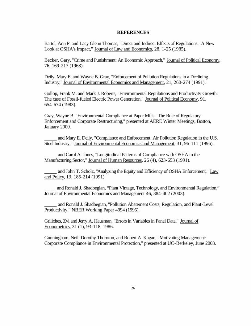
REFERENCES

Bartel, Ann P. and Lacy Glenn Thomas, "Direct and Indirect Effects of Regulations: A New Look at OSHA's Impact," Journal of Law and Economics, 28, 1-25 (1985).

Becker, Gary, "Crime and Punishment: An Economic Approach," Journal of Political Economy, 76, 169-217 (1968).

Deily, Mary E. and Wayne B. Gray, "Enforcement of Pollution Regulations in a Declining Industry," Journal of Environmental Economics and Management, 21, 260-274 (1991).

Gollop, Frank M. and Mark J. Roberts, "Environmental Regulations and Productivity Growth: The case of Fossil-fueled Electric Power Generation," Journal of Political Economy, 91, 654-674 (1983).

Gray, Wayne B. "Environmental Compliance at Paper Mills: The Role of Regulatory Enforcement and Corporate Restructuring," presented at AERE Winter Meetings, Boston, January 2000.

and Mary E. Deily, "Compliance and Enforcement: Air Pollution Regulation in the U.S. Steel Industry," Journal of Environmental Economics and Management, 31, 96-111 (1996).

and Carol A. Jones, "Longitudinal Patterns of Compliance with OSHA in the Manufacturing Sector," Journal of Human Resources, 26 (4), 623-653 (1991).

and John T. Scholz, "Analyzing the Equity and Efficiency of OSHA Enforcement," Law and Policy, 13, 185-214 (1991).

_____ and Ronald J. Shadbegian, “Plant Vintage, Technology, and Environmental Regulation,” Journal of Environmental Economics and Management 46, 384-402 (2003).

and Ronald J. Shadbegian, "Pollution Abatement Costs, Regulation, and Plant-Level Productivity," NBER Working Paper 4994 (1995).

Griliches, Zvi and Jerry A. Hausman, "Errors in Variables in Panel Data," Journal of Econometrics, 31 (1), 93-118, 1986.

Gunningham, Neil, Dorothy Thornton, and Robert A. Kagan, “Motivating Management: Corporate Compliance in Environmental Protection,” presented at UC-Berkeley, June 2003.

26

REFERENCES (cont.)

Harrington, Winston, "Enforcement Leverage when Penalties are Restricted," Journal of Public Economics, 37, 29-53 (1988).

Helland, Eric, "The Enforcement of Pollution Control Laws: Inspections, Violations, and Self-Reporting," Review of Economics and Statistics, 80 (1), 141-153 (1998).

Laplante, Benoit and Paul Rilstone, "Environmental Inspections and Emissions of the Pulp and Paper Industry in Quebec," Journal of Environmental Economics and Management, 31, 19-36 (1996).

Magat, Wesley A. and W. Kip Viscusi, "Effectiveness of the EPA's Regulatory Enforcement: The Case of Industrial Effluent Standards," Journal of Law and Economics, 33, 331-360 (1990).

McGuckin, Robert H. and George A. Pascoe, "The Longitudinal Research Database: Status and Research Possibilities," Survey of Current Business (1988).

Mendeloff, John M. and Wayne B. Gray, “The Effects of Establishment and Inspection Characteristics on the Impacts of OSHA Inspections in Manufacturing,” presented at Law and Society Association Meeting, June 6, 2003.

Nadeau, Louis W., "EPA Effectiveness at Reducing the Duration of Plant-Level Noncompliance," Journal of Environmental Economics and Management, 34 (1), 54-78 (1997).

Scholz, John T., "Cooperation, Deterrence, and the Ecology of Regulatory Enforcement," Law & Society Review, 18, 179-224 (1984).

and Wayne B. Gray, "OSHA Enforcement and Workplace Injuries: A Behavioral Approach to Risk Assessment," Journal of Risk and Uncertainty, 3, 283-305 (1990).

Shadbegian, Ronald J., Wayne B. Gray, and Jonathan Levy, "Spatial Efficiency of Pollution Abatement Expenditures," presented at NBER Environmental Economics session, April 13, 2000.

27

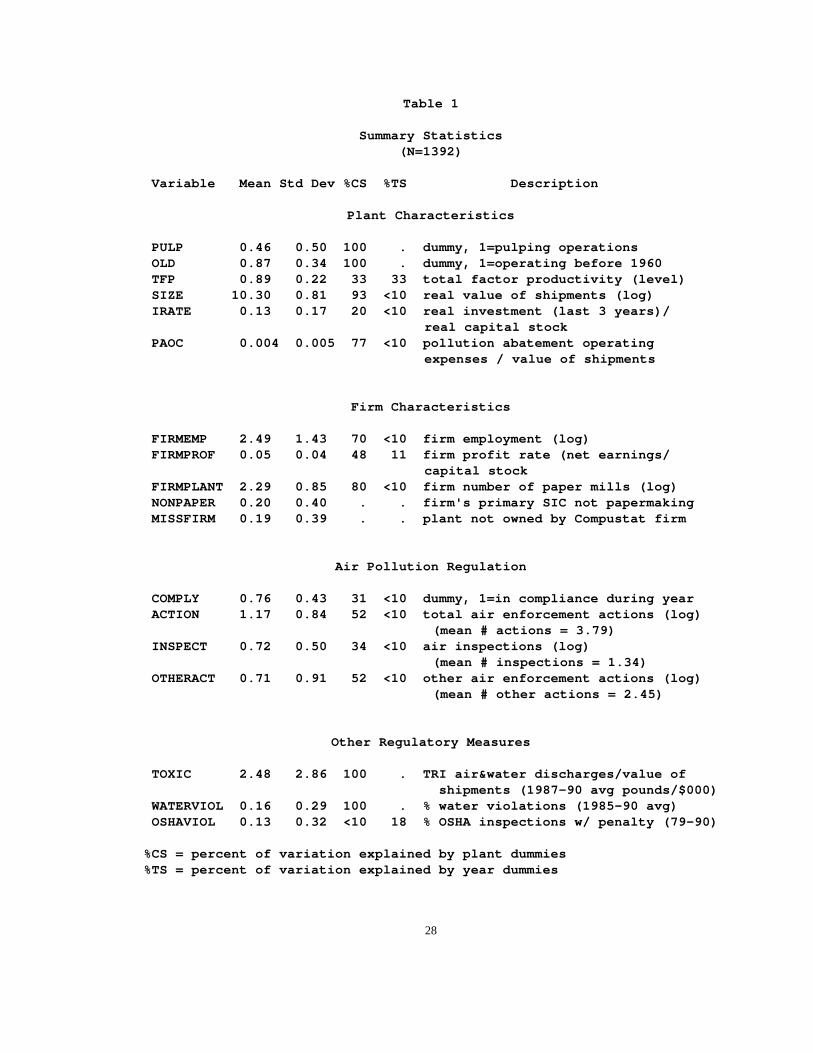
Table 1

Summary Statistics (N=1392)

Variable Mean Std Dev %CS %TS Description

Plant Characteristics

PULP 0.46 0.50 100 . dummy, 1=pulping operations OLD 0.87 0.34 100 . dummy, 1=operating before 1960 TFP 0.89 0.22 33 33 total factor productivity (level) SIZE 10.30 0.81 93 <10 real value of shipments (log) IRATE 0.13 0.17 20 <10 real investment (last 3 years)/

real capital stock PAOC 0.004 0.005 77 <10 pollution abatement operating

expenses / value of shipments

Firm Characteristics

FIRMEMP 2.49 1.43 70 <10 firm employment (log) FIRMPROF 0.05 0.04 48 11 firm profit rate (net earnings/

capital stock FIRMPLANT 2.29 0.85 80 <10 firm number of paper mills (log) NONPAPER 0.20 0.40 . . firm's primary SIC not papermaking MISSFIRM 0.19 0.39 . . plant not owned by Compustat firm

Air Pollution Regulation

COMPLY 0.76 0.43 31 <10 dummy, 1=in compliance during year ACTION 1.17 0.84 52 <10 total air enforcement actions (log)

(mean # actions = 3.79) INSPECT 0.72 0.50 34 <10 air inspections (log)

(mean # inspections = 1.34) OTHERACT 0.71 0.91 52 <10 other air enforcement actions (log)

(mean # other actions = 2.45)

Other Regulatory Measures

TOXIC 2.48 2.86 100 . TRI air&water discharges/value of shipments (1987-90 avg pounds/$000) WATERVIOL 0.16 0.29 100 . % water violations (1985-90 avg) OSHAVIOL 0.13 0.32 <10 18 % OSHA inspections w/ penalty (79-90)

%CS = percent of variation explained by plant dummies %TS = percent of variation explained by year dummies

28

Table 2

Spearman Correlation Coefficients

(N=1392)

PULP OLD TFP SIZE IRATE PAOC

PULP 1.000

OLD (--) 1.000

TFP 0.036 -0.130 1.000

SIZE 0.538 -0.011 0.235 1.000

IRATE -0.048 0.065 0.015 0.042 1.000

PAOC 0.515 0.012 0.006 0.396 -0.001 1.000

COMPLY -0.230 (--) -0.006 -0.179 -0.062 -0.178

ACTION 0.300 -0.071 0.050 0.372 0.006 0.324

TOXIC 0.310 -0.105 0.046 0.255 0.045 0.320

WATERVIOL -0.025 0.149 -0.027 0.288 0.010 0.151

OSHAVIOL 0.039 0.013 -0.090 0.092 0.046 0.056

COMPLY ACTION TOXIC WATERVIOL OSHAVIOL

COMPLY 1.000

ACTION -0.295 1.000

TOXIC -0.094 0.210 1.000

WATERVIOL -0.075 0.093 0.115 1.000

OSHAVIOL -0.116 0.099 0.034 0.143 1.000

Correlations exceeding about .08 are significant at the .05 level. (--) indicates significant negative correlation.

29

Table 3

Basic Compliance Models

(Dep Var = COMP; N=1160)

(3A) (3B) (3C) (3D) (3E) model: Logit Logit Logit OLS F.E.

Plant Characteristics

PAOC 1.064 0.427 0.072 0.879 (0.07) (0.03) (0.02) (0.18)

PULP -0.919 -0.912 -0.170 (-5.07) (-4.73) (-4.94)

OLD (-) (--) (--)

TFP 0.237 0.190 0.024 0.126 (0.59) (0.46) (0.35) (1.11)

IRATE -0.328 -0.219 -0.039 0.019 (-0.75) (-0.50) (-0.50) (0.24)

SIZE -0.303 -0.365 -0.055 0.011 (-2.61) (-2.81) (-2.57) (0.12)

Firm Characteristics

FIRMEMP -0.042 0.120 0.018 -0.057 (-0.38) (1.01) (0.88) (-1.53)

FIRMPROF 2.970 2.468 0.451 -0.029 (1.25) (0.97) (1.01) (-0.06)

FIRMPLANT 0.127 0.052 0.011 -0.073 (1.09) (0.42) (0.51) (-2.09)

NONPAPER (-) (-) (-) (+)

LOG-L -609.72 -645.96 -605.97 pseudo-R2 0.064 0.008 0.070 0.075 0.341

Regressions also include a constant term and year dummies. Firm variables include MISSFIRM.

(-) indicates negative coefficient; (--) indicates significant negative.

30

Table 4

Compliance - Cross-Regulation Effects Logit Models

(Dep Var = COMP; N=1160)

TOXIC

(4A)

-0.000 (-0.02)

(4B) (4C) (4D) Cross-Regulation Effects

0.009 (0.35)

(4E)

0.005 (0.17)

(4F)

-0.031 (-1.33)

WATERVIOL -0.713 (-2.73)

-0.618 (-2.32)

-0.670 (-2.54)

-0.601(-2.58)

OSHAVIOL -0.836 (-4.14)

-0.788 (-3.87)

-0.765 (-3.76)

-0.774(-3.97)

PAOC 0.450 (0.03)

Plant characteristics 4.694 -1.793 1.429

(0.30) (-0.12) (0.09) 2.184

(0.14)

PULP -0.911 (-4.68)

-1.070 (-5.30)

-0.941 (-4.82)

-1.086 (-5.26)

-1.092 (-5.62)

OLD (--) (-) (--) (-) (-)

TFP 0.190 (0.46)

0.118 (0.28)

-0.002 (-0.01)

-0.054 (-0.13)

-0.011 (-0.03)

IRATE -0.219 (-0.50)

-0.321 (-0.72)

-0.194 (-0.43)

-0.292 (-0.65)

-0.401 (-0.90)

SIZE -0.366 (-2.81)

-0.245 (-1.78)

-0.324 (-2.45)

-0.220 (-1.58)

-0.154 (-1.23)

FIRMEMP 0.120 (1.00)

Firm Characteristics 0.099 0.108 0.095

(0.82) (0.90) (0.78) -0.071

(-0.63)

FIRMPROF 2.467 (0.97)

2.152 (0.83)

2.587 (1.00)

2.384 (0.90)

2.917(1.19)

FIRMPLANT 0.052 (0.42)

0.060 (0.49)

0.073 (0.59)

0.077 (0.62)

0.103(0.87)

NONPAPER (-) (-) (-) (-) (-)

LOG-L pseudo-R2

-605.97 0.070

-602.26 0.075

-597.68 0.082

-594.99 0.086

-598.54 0.081

-632.17 0.029

Regressions also include year dummies, a constant term, and MISSFIRM. (-) indicates negative coefficient; (--) indicates significant negative.

31

Table 5

Compliance - Enforcement Measures Logit Models

(Dep Var = COMP; N=1160)

(5A) (5B) (5C) (5D) (5E) (5F)

Enforcement Measures

P(ACTION)-2 -0.213 (-1.40)

ACTION-2 -0.291 (-3.14)

P(INSPECT)-2 0.551 0.429 (1.85) (1.40)

INSPECT-2 -0.080 0.045 (-0.54) (0.30)

P(OTHERACT)-2 0.483 (2.20)

OTHERACT-2 -0.296 (-3.56)

LOG-L -605.01 -601.03 -604.18 -605.82 -601.75 -599.52

pseudo-R2 0.071 0.077 0.072 0.070 0.076 0.079

All models include the complete set of plant and firm characteristics from earlier models, along with year dummies and a constant term.

32

Table 6

Enforcement * Plant Characteristics Logit Models

(Dep Var = COMP; N=1160)

(6A) (6B) (6C) (6D) (6E) (6F)

P(INSPECT)-2 1.047 1.145 -0.065 -0.033 3.827 7.051 (2.24) (2.28) (-0.14) (-0.07) (0.99) (1.51)

P(OTHERACT)-2 0.123 0.171 -1.314 (0.33) (0.41) (-0.51)

PULP*P(INSPECT)-2 -0.792 -1.124 (-1.46) (-1.89)

PULP*P(OTHERACT)-2 0.490 (1.26)

OLD*P(INSPECT)-2 (++) (+)

OLD*P(OTHERACT)-2 (+)

SIZE*P(INSPECT)-2 -0.309 -0.628 (-0.85) (-1.42)

SIZE*P(OTHERACT)-2 0.175 (0.72)

LOG-L -603.08 -599.76 -602.89 -600.62 -603.82 -600.75

pseudo-R2 0.074 0.079 0.074 0.078 0.073 0.078

All models include the complete set of plant and firm characteristics from earlier models, along with year dummies and a constant term.

33

Table 7

Enforcement * Firm Characteristics Logit Models

(Dep Var = COMP; N=1160)

(7A) (7B) (7C) (7D) (7E) (7F)

P(INSPECT)-2 0.458 0.458 0.685 1.311 0.829 1.604 (1.18) (1.67) (1.47) (2.55) (1.32) (2.35)

P(OTHERACT)-2 0.402 -0.713 -0.862 (1.00) (-1.84) (-1.65)

PROF*P(INSPECT)-2 2.464 0.529 (0.38) (0.07)

PROF*P(OTHERACT)-2 0.644 (0.14)

EMP*P(INSPECT)-2 -0.062 -0.445 (-0.37) (-2.29)

EMP*P(OTHERACT)-2 0.488 (3.89)

PLANTS*P(INSPECT)-2 -0.142 -0.643 (-0.50) (-2.00)

PLANTS*P(OTHERACT)-2 0.587 (2.94)

LOG-L -604.11 -601.73 -604.11 -593.39 -604.05 -596.80

pseudo-R2 0.072 0.076 0.072 0.089 0.072 0.084

All models include the complete set of plant and firm characteristics from earlier models, along with year dummies and a constant term.

34

Figure 1

Impact of Shift in Regulation on Optimal Compliance

MB=MB(Xp,Xf,REGS,X*REGS)

MC=MC(Xp,Xf)

$ $ $

MC1MB1’= MB2’

MC2

MB1=MB2

Figure 1a

Same MB shift, Different MC levels, Same MC slope

Compliance

MC2

MC1

MC1=MC2

MB1’=MB2’

MB1=MB2

MB2’

MB1=MB2

MB1’

Figure 1b

Same MB shift, Different MC levels, Different MC slopes

Figure 1c

Different MB shifts (MB1 more sensitive), Same MC

Compliance Compliance

35