Working Paper Series

ISSN 1518-3548

Credit Channel with Sovereign Credit Risk: an Empirical Test Victorio Yi Tson Chu

September, 2002

ISSN 1518-3548

CGC 00.038.166/0001-05

Working Paper Series

Brasília

n. 51

Sep

2002

p. 1 – 28

Working Paper Series

Edited by: Research Department (Depep) (E-mail: workingpaper@bcb.gov.br) Reproduction permitted only if source is stated as follows: Working Paper Series n. 51. Authorized by Ilan Goldfajn (Deputy Governor for Economic Policy). General Control of Subscription: Banco Central do Brasil

Demap/Disud/Subip

SBS – Quadra 3 – Bloco B – Edifício-Sede – 2º subsolo

70074-900 – Brasília (DF)

Telefone: (61) 414-1392

Fax: (61) 414-3165

The views expressed in this work are those of the authors and do not reflect those of the Banco Central or its members. Although these Working Papers often represent preliminary work, citation of source is required when used or reproduced. As opiniões expressas neste trabalho são exclusivamente do(s) autor(es) e não refletem a visão do Banco Central do Brasil. Ainda que este artigo represente trabalho preliminar, citação da fonte é requerida mesmo quando reproduzido parcialmente. Banco Central do Brasil Information Bureau Address: Secre/Surel/Diate

Edifício-Sede – 2º subsolo

SBS – Quadra 3 – Zona Central

70074-900 Brasília (DF)

Phones: (5561) 414 (....) 2401, 2402, 2403, 2404, 2405, 2406

DDG: 0800 99 2345

FAX: (5561) 321-9453

Internet: http://www.bcb.gov.br

E-mails: cap.secre@bcb.gov.br

dinfo.secre@bcb.gov.br

3

Credit Channel with Sovereign Credit Risk: An Empirical Test*

Victorio Yi Tson Chu**

Abstract

According to Bernanke and Gertler (1995), the Credit Channel amplifies the traditional monetary transmission and this amplification effect comes through the firm’s external finance premium, which is a wedge between the expected return for the funds generated internally and the costs of funds raised externally to the firm. Traditionally, this wedge is the bank loan spread but we extend this concept to include the sovereign (country) credit risk and name it, Extended Credit Channel. Armed with this new concept and using a set up model, we estimate two econometric equations for the Brazilian economy after its inflation stabilization program. These two econometric equations measure: (1) the effects of the pure money channel (real interest rates and compulsory reserve requirements on demand deposits) and the extended credit channel (country credit risk and bank loan spread) on the economy’s production, and (2) the impacts of the real interest rates, compulsory reserve requirements on demand deposits, and country credit risk on the bank loan spread. Both equations coefficients signs conform to the expected theoretical model. With the results of the estimated equation (1), we define a Product Loss Index Number to compare these two transmission channels (extended credit and pure monetary). This comparison shows that the extended credit channel is as relevant as the pure monetary channel. Keywords: Credit Channel, Sovereign Credit Risk, Reserve Requirements and Bank Loan Spread. JEL Classification: E44, E50, N16.

* The author thanks, without implicating, Eduardo L. Lundberg, Márcio I. Nakane, Eduardo Tonooka for their valuable comments and, Sérgio Mikio Koyama for his assistance with the data. The views expressed here are solely the responsibility of the author and do not reflect those of the Central Bank of Brazil. ** Research Department, Central Bank of Brazil. E-mail address: victorio.chu@bcb.gov.br

4

In his survey, Hubbard (1994) argues that “... the terms “money view” and “credit view”

are not always well defined in theoretical debates over the transmission mechanism of

monetary policy.” These views are also denominated as a “money view” channel and

“credit view” channel.

The traditional or “pure” money channel is defined as the transmission mechanism

through basic interest rates and deposit reserve requirements. And, in this paper, we will

define the credit channel according to the concept found in Bernanke and Gertler

(1995), as a monetary transmission mechanism channel that is a companion to the

“money” channel, particularly, the direct effects of monetary policy on interest rates that

amplifies the borrower’s external finance premium. This borrower’s external finance

premium is the difference between the costs of the loans interest rate and the cost of

these funds for the lenders, namely the banks. Then, the credit channel is not seen as a

freestanding or parallel to the money channel.

Most of the emerging markets are large borrowers in the international financial system;

hence they also face an external finance premium that is usually quoted as a spread over

the US Treasury bonds.

Before proceeding, we must address the following questions: What is the importance of

the credit channel? And how relevant is the sovereign credit risk as a component of the

credit channel?

Thus, in this article we tackle this sovereign external finance premium by extending the

traditional credit channel to include the country or sovereign credit risk.

What lies behind this extension of the credit channel is the effect associated to a

country’s economy when faced with adverse changes on its external finance premium.

As it is well documented in many articles, like Hermalin and Rose (1999), Reinhart

(2002), and Magalhães, Moreira and Rocha (2002), the deterioration of a country’s

credit rating, which translates in an increase of its external finance premium, is not the

cause for decline of its macroeconomic or credit conditions but it is just mirroring the

worsening of the country’s economic risk or its economic expectations. Rigobon (2001)

5

shows how a country’s upgrade to investment grade credit rating increases the inflow of

foreign funds, improving the overall condition of the economy. When well managed,

this improvement to investment grade credit rating creates a virtuous circle: increasing

investment, the economy grows, credit rating betters up which increases the inflow of

funds and so on.

Therefore, the motivation for this paper is to answer the following set of questions:

(Q1) What are the magnitude of the effects on income derived from this difference

between the funds cost of the financial intermediaries, namely the banks, and the cost of

the loans to borrowers?

(Q2) How relevant is sovereign credit risk premium effect on the credit channel and on

the economic activity?

Our theoretical model is based on the economic model presented in Chu and Nakane

(2001), which was built on the loan interest-rate clearing-price framework fashioned by

Bernanke and Blinder (1988). And it was adapted to suit for a variable representing the

difference between the banks’ loans interest rate and the cost of these resources,

namely, the bank loan spread.

The first empirical equation was based on a cointegration model with an error correction

term, and estimated the relationship between the real income (using the Industrial

Production Index as a proxy) and the components of the pure money channel (legal

reserves on demand deposits and real interest rates) and the extended credit channel

(bank loans spread and sovereign country credit risk) for Brazil after its Inflation

Stabilization Program in July 1994.

Our second empirical equation, also based on a cointegration model with an error

correction term, searches for a relation between the bank loan spread and those other

components of the monetary transmission, namely, the legal reserves, interest rates and

country credit risk.

After estimating these two equations, we calculate the sensibility of the dependent

variables to changes in the explanatory variables. We create a Product Loss Index to

6

compare the impact of the pure money channel and the extended credit channel, which

results that the effects of the extended credit channel can be as relevant as the pure

money channel.

The paper is divided in four parts. First, we make a short description of the model found

in Chu and Nakane (2000) and adapt it for the bank loans spread. Second part describes

the data for Brazil used for the empirical test. In the third part, we present the

econometric model and the estimated equations and discuss the results. Finally, the last

part is the conclusion.

1. The Model

In this section we will make a short description of the theoretical model presented in

Chu and Nakane (2001).

The main hypotheses concerning this economy with four agents: banks, government,

households and firms are:

H1) The monetary authority follows an inflation-targeting regime and determines

two policy instruments: a short-term nominal interest rate and the required reserve ratio

on demand deposits (α). In the short-term and under inflation targeting regime, there is

no uncertainty about the inflation, therefore the monetary authority can control the real

interest rate rB = _

Br , where _

Br is the real interest rate on public bonds. These two policy

instruments are assumed to be exogenous in the model. And the supply of public bonds

Bg is infinitely elastic at the real interest rate _

Br .

H2) Let S (y, rB) be the households real savings and y the real income. The partial

derivatives are 0>yS and 0>Br

S .

H3) Firms finance their investments I (rB, rL) through bank loans that cost the loan

interest rate rL, where 0<Br

I and 0<Lr

I . And I (rB, rL) = S (y, rB). The variable banking

7

loan spread (γ) represents the difference between banking loan interest rate and the basic

interest rate paid by the public bonds.

H4) Banks’ have only demand deposits, no capital and hold three assets: legal

reserve requirements on demand deposits (R), public bonds (Bb) and loans (Lb). Bank’s

balance sheet will be equal to:

(1) R + Bb + Lb = Db

Where Db is banks’ total deposits. It is assumed that the banks accept passively all the

deposits demanded by the non-bank public. And the non-banks public deposits demand

function is Dd(y, rB) with 0>dyD and 0<d

rBD as its partial derivatives. The banks do not

pay interest for the demand deposits that are subject to legal reserve requirements and

they do not carry excess reserves beyond the minimum established by the monetary

authority.

(2) R= α Db

Let Bb(σ, rL), where σ is variable that represents the economy’s risk. The assumption

for its partial derivatives is 0>bBσ and 0<brL

B . It is assumed that the demand for

public bonds is totally inelastic with respect to its own interest rate.

Applying Bb(σ, rL) in equation (1) and substituting for (2) we will have the following

banks’ supply of loans function:

(3) Lb = (1-α) Db - Bb(σ, rL)

The non-bank public’s demand for bank loans is denoted by Ld(rL, y) with partial

derivatives 0<drL

L and 0>dyL .

With these assumptions, the market clearing condition for the goods market corresponds

to the IS schedule with a negative slope in the (rL, y) plan:

8

(4) 0<=Lr

y

IS

L

I

S

dy

dr

The market clearing conditions for the deposits and bank loans represented in a single

schedule is made by using equation (3) with Db = Dd(y, rB) and Lb = Ld (rL, y), then,

(5) (1- α)Dd(y, rB) - Bb(σ, rL) = Ld(rL, y)

Equation (5) provides the set of (rL, y) that assures the simultaneous equilibrium in the

deposit and loan markets represented by the schedule DL. This DL schedule can have a

positive or negative slope in the (rL, y) plan:

(6) dr

br

dy

dy

DL

L

LLLB

LD

dy

dr

+−−

=)1( α ≷ 0

The sign uncertainty comes from the numerator’s unknown sign result, but in any event,

the DL slope is assumed to be greater than the IS slope.

The economy’s general equilibrium is represented in Figure 1. With a positive slope for

DL and rL* and y*, represent, respectively, the equilibrium values for rL and y.

rL

D L

r*L

I S

y* y

Figure 1: The Economy’s General Equilibrium.

9

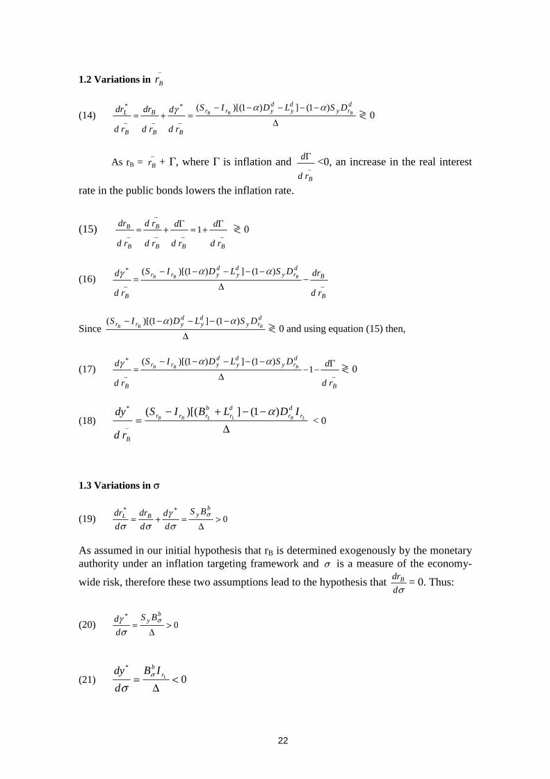
The model’s exogenous variables are α, r*B, and σ. Table 1 summarizes the comparative

static results for the model1.

Variable λ dy*/dλ dr*L/dλ

α - +

_

Br - ?

σ - +

Table 1: Comparative Static and _

Br is the basic real interest rate.

After this brief description of Chu and Nakane (2001), we will adapt their model for the

bank loan spread γ*, where γ* = r*L – rB , by replacing r*

L for (γ* + rB) and deriving the

equations found in the appendix of Chu and Nakane (2001) for the bank loan spread γ*

variable.

In Table 2, we present these results. And in the Appendix, it is shown the mathematical derivation of those equations with the loan spread γ*.

Variable λ dy*/dλ dγ*/dλ

α - +

_

Br - ?

σ - +

Table 2: Comparative Static with y* and γ*.

The variable _

Br is the basic real interest rate.

The signs of derivatives related to the spread (γ*) are intuitive:

An increase in α results in additional compulsory reserve requirements for demand

deposits, meaning that the banks will have a lower volume of money for lending

purposes, therefore we will have a higher γ*. And an opposite situation happens when α

1 The proofs of the results presented in Table 1 appear in the Appendix of Chu and Nakane (2001).

10

decreases, with a larger volume of funds resulting in a lower γ*. Figure 2 shows

graphically the effects of an increase of α.

rL

D L’

r**L= rB + γ**

DL

r*L= rB + γ*

I S

y** y* y

Figure 2: Effects of Increasing the Required Reserve Ratio (α**>α*) with γ**> γ*.

Lowering the economy-wide risk σ leads the banks to reduce their demand for public

bonds freeing resources for loans, this will move the DL curve to the right, resulting in

an opposite situation from Figure 2. This effect is shown graphically in Figure 3.

rL

D L

r*L= rB + γ*

DL’

r**L = rB + γ**

IS

y* y** y

Figure 3: Effects of Decreasing the Economy-wide Risk (σ*>σ**) with γ*> γ**.

Increases in the variables α, _

Br and σ result in a shift of the DL schedule to the left or

upward that lower the y* for the same IS schedule.

11

2. The Data

We made an empirical test with the data from the Brazilian economy. Our test sample

starts in August/1994 and goes till September/2001, consisting of 86 monthly

observations. The Brazilian hyperinflation stabilization plan started in July/1994, then

we choose August/1994 as starting month, because there were some inflation residuals

contaminating the July inflation index. These data contain the following variables:

Country Credit Risk (Risk)– it consists of the monthly geometric average price of the

Brazilian foreign debt (C-Bond) and is measured as annual spread over the U.S.

Treasury Bonds. This spread measures the country credit risk or, in other words, the

Brazilian sovereign credit risk. The Augmented Dickey-Fuller test for unit root was

performed and could not reject that the series is integrated of order one, I(1).

Spread (S)– it is the banking loan monthly spread published in the monthly and annual

report2 produced by the Brazilian Central Bank. It is basically a weighted average of

fixed loans and credit instruments offered by the main private banks in Brazil. The unit

root tests indicated that this series is I(1).

Real Interest Rates plus one (1+rB) – where rB is the geometric average monthly basic

interest rate of the economy determined by the Brazilian Central Bank SELIC (i)

divided by the General Price Index (IGP-DI) published by FGV. The unit root test

rejected at 5% significance, meaning that the series is stationary at series level, I(0).

Product (Y) – it is represented by the monthly Industrial Production Index collected by

IBGE (Brazilian Institute of Geography and Statistics) and it was seasonally adjusted

by the multiplicative X-11 methodology. Applying the unit root tests resulted that the

series is integrated of order one, I(1).

Compulsory Reserve Requirements (α) – it is the legal reserve requirement for the

banks’ demand deposits. These are the reserves, as a percentage of demand deposits that

12

the banks are obliged to deposit at the monetary authority. Unit root tests indicated that

the series is integrated of order one, I(1).

Figure 4 presents a graphic with the Risk (C-Bond as % a.y. spread over the U.S.

Treasury Bonds) and the behavior of the Industrial Production Index Seasonally

Adjusted. It is possible to see that the valleys of the C-Bond are accompanied by an

increase of the Industrial Production, suggesting a negative relationship between these

two variables.

2 4 6 8

10 12

100

110

120

130

140

95 96 97 98 99 00 01

. Figure 4: Dotted Line - Risk % a.y. over Treasury

Bold Line - Industrial Production Season Adjusted.

Figure 5 is a graphic of the Loan Spread (% a.m.) versus the Compulsory Reserve

Requirements as a percentage of Total Demand Deposits. It can be seen that the drop of

the legal reserve requirements is accompanied by a reduction of the loan spread.

2 Banco Central do Brasil, “Notas dos Juros e Spread Bancário no Brasil” (monthly report) and “Juros e Spread Bancário no Brasil” (report for the years 1999, 2000 and 2001). These reports also describe the calculus methodology for these loan spreads.

13

40

50

60

70

80

90

2

3

4

5

6

95 96 97 98 99 00 01

Figure 5: Dotted Line - % Compulsory Reserve

Bold Line - Loan Spread % a.m.

3. Empirical Model

3.1. Empirical Model for the Product (Y)

From Table 2, the empirical model for the dependent variable product Y, which has the

Industrial Production Index Seasonally Adjusted as its proxy, is explained using the

explanatory variables from Table 2: compulsory reserve requirements (α), real interest

plus one (1+ rB) and (risk) measured by the Brazilian sovereign credit risk (C-Bond);

with an additional varaible: bank loan spread (S).

The Johansen test was performed up to 12 lags for a group of these 5 variables and co-

integration could not be rejected for at least 3 co-integration vectors.

The presence of co-integration resulted in the necessity of an Error Correction Term

(ECTY) for our econometric model. The specification of ECTY3 is:

3 The econometric program that we used did not provide the standard deviation for the coefficients of the deterministic trend (*) and the intercept (**).

14

81037.5002053.0015774.0ln348324.0)1ln(62011.11ln077083.0ln −−−−+++= Trendtt

StB

rt

Riskt

Yt

ECTY α (0.01589) (1.39767) (0.07020) (0.01866) (*) (**)

Where the term Trend represents a linear trend variable.

The econometric model for the product Y was:

(7)

10 0

1 0 0

lnln

)1ln(lnln)ln(

−= =

−−

= = =−−−

∑ ∑

∑ ∑ ∑

+∆+∆+

++∆+∆+∆=∆

t

n

j

n

jjtjjtj

n

j

n

j

n

jjtBjjtjjtjt

ECTYS

rRiskYY

δωαβ

ωζξ

The econometric test was performed assuming all variables as I(1), including the

variable real interest rate plus one (1+ rB). The difference operator for the variables

logarithm is represented by the ∆ operator.

The estimation of the coefficients of the econometric equation for the product Y,

represented by Industrial Production Index Seasonally Adjusted, is shown in Table 4

below. The sign for the sum of the coefficients for each variable accords to the

prediction of our theoretic model. The discussion of these results are presented in the

following sub-section 3.3.

Table 4: Estimated Econometric Equation for Product Y

Dependent Variable: ∆lnYt Variable Coefficient Std. Error t-Statistic

∆lnYt-1 -0.437323 0.086003 -5.084998 ∆lnYt-4 -0.149864 0.085990 -1.742821

∆lnRiskt -0.067580 0.023288 -2.901918 ∆ln(1+ rB)t-2 0.735783 0.263039 2.797237 ∆ln(1+ rB)t-9 -0.735944 0.248503 -2.961508 ∆ln(1+ rB)t-12 -0.548211 0.238608 -2.297537 ∆lnSpreadt-1 -0.120808 0.054495 -2.216851

∆lnαt 0.145041 0.077130 1.880482 ∆lnαt-8 -0.167872 0.076972 -2.180958

ECTYt-1 -0.070964 0.024932 -2.846265 Adjusted R-squared: 0.491663 Durbin-Watson stat: 2.190872

Our tests did not reject normality (Jarque-Bera), homocedasticity (Arch(1) and White)

and residuals are not correlated.

15

3.2. Empirical Model for the Spread (S)

The empirical model for the dependent variable Spread (S), which is a monthly rate,

consisted of three variables: compulsory reserve requirements (α), real interest plus one

(1+ rB) and MRisk, which is a conversion of C-Bonds annual spread over U.S. Treasury

Bonds to monthly spread over U.S. Treasury Bonds. Equation (8) shows mathematically

the conversion of the annual Risk (Cbond) to monthly risk rates (MRisk):

(8) 121

)1( RiskMRisk +=

We performed the Johansen test up to the 12 lags for a set of these 4 variables and co-

integration could not be rejected for at least 2 co-integration vectors.

The existence of co-integration produced the need of an Error Correction Term (ECTS)

for our econometric model. The specification of ECTS is:

218101.060048.0)1ln(43029.17ln693660.0ln −−+−−= ttBttt rMRiskSpreadECTS α

(0.11199) (3.29866) (0.14303)

Except for ln(1 + rB) which is I(0), those other 3 variables, Spread (S), compulsory

reserve requirements (α) and monthly risk rates (MRisk) are all I(1). And the difference

operator for the variables logarithm is represented by the ∆ operator.

The econometric model for the Spread was:

(9)

10 0

)1ln(ln

1ln

1)ln(tan)ln(

−∑=

+∑= −+∆+−∆+

∑=

+−∆+∑= −∆+=∆

tECTS

n

j

n

jjt

rjjt

MRiskj

n

jjtj

n

jjt

SpreadtConst

Spread

B δωζ

αξ

Our final estimation for the coefficients of the econometric equation for the Spread is

shown in Table 5.

16

Table 5: Estimated Econometric Equation for the Spread

Dependent Variable: Spread

Variable Coefficient Std. Error t-Statistic Constant 0.024429 0.010781 2.266037

∆lnSpreadt-2 0.236747 0.094574 2.503298 ∆lnSpreadt-3 -0.160601 0.099413 -1.615494 ∆lnSpreadt-4 -0.266109 0.099319 -2.679329 ∆lnSpreadt-7 -0.176287 0.094000 -1.875400 ∆lnSpreadt-11 -0.231517 0.083909 -2.759128 ∆lnMRiskt-8 0.115184 0.043782 2.630857

∆lnαt 0.339996 0.157733 2.155515 ∆lnαt-5 0.451151 0.146564 3.078177 ∆lnαt-6 0.318329 0.145719 2.184548

∆ln(1+ rB)t 2.200057 0.555877 3.957810 ∆ln(1+ rB)t-1 -1.444039 0.729013 -1.980814 ∆ln(1+ rB)t-2 -1.100265 0.621179 -1.771252 ∆ln(1+ rB)t-3 2.261766 0.593387 3.811619 ∆ln(1+ rB)t-5 -0.969302 0.506735 -1.912838 ∆ln(1+ rB)t-7 1.123173 0.593310 1.893061 ∆ln(1+ rB)t-8 -2.725414 0.555900 -4.902705 ∆ln(1+ rB)t-12 -1.250886 0.486525 -2.571063

ECTSt-1 -0.062721 0.025932 -2.418649 Adjusted R-squared: 0.454738 Durbin-Watson stat: 2.272964

The performed tests for normality (Jarque-Bera), homocedasticity (Arch(1) and White)

were not rejected and residuals are not correlated.

Also, the Wald test with the null hypothesis for the sum of coefficients of ∆ln(1+ rB) = 0

resulted in its rejection at 1% significance, as presented in Table 6.

Table 6: Wald test results for the sum of the coefficients of ∆ln(1+ rB).

Wald Test: Null Hypothesis: C(11)+C(12)+C(13)+C(14)+C(15)+C(16)+C(17)+C(18)=0 F-statistic 7.536553 Probability 0.008152 Chi-square 7.536553 Probability 0.006046

3.3 Discussion of the Results

Our empirical results for the Brazilian economy are in accordance with what’s predicted

by the Chu and Nakane’s (2001) theoretical model. And a sensibility analysis for a

medium term economic horizon is presented in Tables 7 and 8, respectively, for the

estimated Product Equation and Bank Loan Spread Equation.

17

(1) The product Y equation

The coefficients signs are: negative for Risk (CBond), negative for real interest rate,

negative for the bank loan spread and negative for α - compulsory reserve requirements

for demand deposits.

Table 7: Sensibility analysis for the coefficients of the Estimated Product Equation.

Industrial Production Index: annual rate rounded to second decimal {(Yt/Yt-1)-1}Risk Increase of 10% of Risk -40 b.p.(1+ rB)4 Increase of 10% of rB(t) with rB(t-1) = 8% a.y, depends on level of rB(t-1) -25 b.p.Spread A 10% Spread Increase. -72 b.p.α Increase of 10% compulsory reserve requirement. -14 b.p.b.p. = basis point

Since the range of our risk (C-Bond) as spread over the Treasury is between 600 b.p. to

1,000 b.p. then a 10% increase in risk, representing an additional of 60 b.p. to 100 b.p.,

translates into an estimated drop of – 40 b.p. in the year product.

The effects of the real interest rate is approximate, because our variable is (1+ rB) and

not only rB, hence, at the level of rB = 8% a.y. which corresponds to a value of 1+ rB (=

1.08) and 10% of it amounts nearly 100 b.p. a year, resulting in an estimated loss of -25

b.p. over the country’s yearly production.

Since the bank loan spread is very high in Brazil, a 10% increase on the loan spread

equals an addition of a number within the range of 350 b.p. to 750 b.p., which will have

an estimated negative impact of –72 b.p. on the year’s production. And for α, the

compulsory reserve requirement on demand deposits, its effects is smaller, in the

present case of α = 45% of the demand deposits, a 10% increase equals an addition of

450 b.p. resulting in an estimated negative impact on the yearly production of –14 b.p.

4 The result is approximate since to find the ln((1+Xt/(1+Xt-1)) in the case of real interest rates depends on the exact number of Xt and Xt-1.

18

In summary, we can see that the variable that has the largest negative impact on the

Industrial Production Index is the Sovereign Credit Risk (C-Bond), which for a 10%

increase in the sovereign risk (with the risk on the range of 600 b.p. to 1,000 b.p. over

the US Treasury bonds) generates a loss on the production index in the range of –0.6666

to –0.45.

Defining PLIN as Product Loss Index Number6, this index number represents how

many basis points of yearly production loss for each basis point change of the

explanatory variable. Thus, after the sovereign credit risk, the real interest rate (at the

initial interest rate in the neighborhood of 8 % a year) will have a negative impact of –

0.25 on PLIN and the bank loan spread, for the spread at 34.495% a year, will result in a

product loss index number of -0.2087. And the smallest impact on PLIN for a 10%

increase in the variable is related to the compulsory reserve requirement, at today’s

value of α = 45% to α = 49.5% of the demand deposits, this will produce a negative

change of -0.03111 to the production loss index number. Table 8 summarizes all the

impacts on the product loss index number (PLIN) for an adverse change in the

macroeconomic variable.

Table 8: Variables impact on the product in terms of a loss index number.

Product Loss Index Number: Estimated Product Loss Index Range

Increase of 10% of Risk (Country Credit Risk) range: 60 to 100 b.p. -0.66667 -0.40

Increase of 10% of Rb(t), with initial Rb(t-1) = 8% a.y. (Variations depend on initial Rbt-1)

-0.25 -0.25

Increase of 10%, for annual spread (initial spread of 34.49%) -0.2087 -0.2087

Increase of 10% for α (compulsory reserve requirement) initial α(t-1) = 45% -0.03111 -0.03111

Table 9 below compares the sum of the product loss index number for those two

channels of transmission: Extended Credit Channel (with the variables: Country Credit

Risk and Bank Loan Spread) and Pure Monetary Channel (with the variables: real

interest rates and compulsory reserve requirements). It can be seen that the extended

credit channel affects sensitively on the yearly production. Since the overall impact

5 The division of the loss in b.p. per 10% change of the variable in b.p. generates a loss index number, for instance, (-40 b.p./60b.p.) equals –0.666 for the upper limit of the risk variable impact. 6 The Product Loss Index sign is negative because in the coefficients signs of the econometric equation are negative.

19

depends on the initial state, we can say, at the very least, that the Extended Credit

Channel affects the economy as much as the pure monetary channel.

Table 9: Comparing the effects of Extended Credit Channel and Pure Monetary Channel

Sum Of Product Loss Index Number: Estimated Range Extracted from Tables 7 and 8

Extended Credit Channel effects (Country Credit Risk and Bank Loan Spread) -0.87537 -0.6087 Pure Monetary Channel effects (real interest rates and compulsory reserve requirements)

-0.28111 -0.28111

(2) The bank loan spread (S) equation

The coefficients signs are: positive for Risk (CBond), positive for real interest rate and

positive for α - compulsory reserve requirements for demand deposit.

Table 10: Sensibility analyses for the coefficients of the

Estimated Loan Spread Equation

Spreadt – Spreadt-1, where Spreadt-1= 34.49% a.y, and rounded to second decimalRisk Increase of 10% of Risk (C-Bond) 77 b.p.

(1+ rB) Increase of 10% of rB(t) with rB(t-1) = 8% a.y, depends on level of rB(t-1) 57 b.p.

α Increase of 10% compulsory reserve requirement 293 b.p.

b.p. = basis point

Repeating the same analysis for the bank loan spread within the same 10% range

increase assumed for those explanatory variables in the product equation described

above, and from a initial bank loan spread of 34.49% a year, we get the following

results:

For a range of 60 b.p. to 100 b.p. addition limits to the risk (C-Bond) variable at the

annual rate, we will have an estimated annual spread increase of 77b.p.

The additional real interest rate, considering that the actual variable is (1 + rB) and the

initial rB is 8% a year, is 57 b.p. for the annual rate.

Of these three variables (risk, real interest rate and reserve requirements), the largest

impact on the bank loan spread comes from the legal reserve requirements. An

additional 10% of the compulsory reserve requirements on demand deposits (α), which

20

at present moment stands at 45% rate, resulting in a new α of 49.5% rate will increase

the annual bank loan spread by an estimated 293 b.p.

4. Conclusion

This paper is a follow-up of a theoretic model contained in Chu and Nakane (2001) and

makes an empirical test based on that theoretical model. The monetary authority has

control over two policy instruments: short term real interest rate and the compulsory

reserve requirements for the demand deposits. More specifically, we cover empirically

the effects of transmission to the bank loans called credit channel and, extend it to

include the sovereign country credit risk measured, using C-Bonds, as a spread over the

US Treasury bonds.

The impact on the Brazilian economy of this extended credit channel, which is the sum

of the effects of the bank loans spread and the sovereign credit risk (as a proxy for an

economy-wide risk) can be as relevant as the pure money channel (interest rates and

legal reserve requirements).

Hence, in determining the effects of the credit channel for emerging countries

economies it is important to include a parameter that indicates the expected risk of the

economy. A useful proxy for this risk is the sovereign country credit risk.

21

Appendix The results from the Appendix of Chu and Nakane (2001) are presented and they will be used to generate new equations for the spread γ* variable. Given the two equations represented by the IS and DL I(rB, rL) = S(y, rB)

(1- α)Dd(y, rB) - Bb(σ, rL) = Ld(rL, y) Let ∆ the system’s Jacobian determinant solved at the equilibrium, which is equal to:

0)( >

−++=∆dy

dr

dy

dr LLLBI

ISDL

dr

brr LLL

Since the DL slope is assumed to be less steep than the IS slope then the ∆ sign is positive. Knowing that (10) r*L= rB + γ*

And by equation (10), assuming that αd

drB = 0, and substituting and deriving the

equations below, comes: 1.1 Variations in α

(11) 0*

>∆

= yd

LSD

d

dr

α

0***

>∆

==+= yd

BLSD

d

d

d

d

d

dr

d

dr

αγ

αγ

αα

(12) 0*

>∆

= yd SD

d

d

αγ

(13) 0*

<∆

= Lrd ID

d

dy

α

22

1.2 Variations in _

Br

(14) ∆

−−−−−=+=

dry

dy

dyrr

BB

B

B

L BBBDSLDIS

rd

d

rd

dr

rd

dr )1(])1)[((_

*

__

* ααγ ≷ 0

As rB = _

Br + Γ, where Γ is inflation and _

Brd

dΓ <0, an increase in the real interest

rate in the public bonds lowers the inflation rate.

(15) ___

_

_1

BBB

B

B

B

rd

d

rd

d

rd

rd

rd

dr Γ+=Γ+= ≷ 0

(16) __

* )1(])1)[((

B

Bdry

dy

dyrr

B rd

drDSLDIS

rd

d BBB −∆

−−−−−=

ααγ

Since ∆

−−−−− dry

dy

dyrr BBB

DSLDIS )1(])1)[(( αα ≷ 0 and using equation (15) then,

(17) __

*

1)1(])1)[((

B

dry

dy

dyrr

B rd

dDSLDIS

rd

d BBB Γ−−∆

−−−−−=

ααγ ≷ 0

(18) ∆

−−+−= LBLLBB r

dr

dr

brrr

B

IDLBIS

rd

dy )1(])[((_

* α < 0

1.3 Variations in σ

(19) 0**

>∆

=+=b

yBLBS

d

d

d

dr

d

dr σ

σγ

σσ

As assumed in our initial hypothesis that rB is determined exogenously by the monetary authority under an inflation targeting framework and σ is a measure of the economy-

wide risk, therefore these two assumptions lead to the hypothesis that σd

drB = 0. Thus:

(20) 0*

>∆

=b

y BS

d

d σ

σγ

(21) 0*

<∆

= Lrb IB

d

dy σ

σ

23

References

Banco Central do Brasil (1999, 2000 and 2001) ‘Juros e Spread Bancário no Brasil’ (yearly report).

Banco Central do Brasil (1999, 2000 and 2001) ‘Notas dos Juros e Spread Bancário no Brasil’ (monthly report).

Bernanke, B. S. and Blinder, A. S. (1988) ‘Credit, money, and aggregate demand’. American Economic Review, Papers and Proceedings, 78, 435–439.

Bernanke, B. S. and Gertler, M. (1995) ‘Inside the black box: the credit channel of monetary policy transmission.’ The Journal of Economic Perspectives, Vol. 9 Issue 4, 27-48.

Campbell, J. Y. and Mankiw, N. G. (1989). ‘Consumption, income, and interest rates: reinterpreting the time series evidence’. In Blanchard, O. J. and Fischer, S., editors, NBER Macroeconomics Annual 1989. MIT Press, Cambridge, MA.

Chu, V.Y.T. and Nakane, M.I. (2001). ‘Credit channel without the LM curve’. Economia Aplicada, vol.5, Nº 1, 213-227.

Hallsten, K. (1999). ‘Bank loans and the transmission mechanism of monetary policy’. Sveriges Riksbank Working Paper No. 73. Sveriges Riksbank. Stockholm.

Hermalin, B. E. and Rose, A. K. (1999), ‘Risks to lenders and borrowers in international capital markets’. NBER Working Paper No. 6886.

Hubbard, R.G. (1994), ‘Is there a ‘Credit Channel’ for monetary policy?’. NBER Working Paper No. 4977.

Kashyap, A. K. and Stein, J. C. (1994). ‘Monetary policy and bank lending’. In Mankiw, N. G., editor, Monetary Policy. University of Chicago Press, Chicago.

Magalhães, R., Moreira, A.R.B. and Rocha, K. (2002). ‘Determinantes do spread brasileiro: uma abordagem estrutural’.Seminários DIMAC No. 90 IPEA.

Miron, J. A., Romer, C. D., and Weil, D. N. (1994). ‘Historical perspectives on the monetary transmission mechanism’. In Mankiw, N. G., editor, Monetary Policy. University of Chicago Press, Chicago.

Nakane, M. I. (2000) ‘Canal de crédito: evidências para o Brasil’, handout, Banco Central do Brasil DEPEP Seminars.

Puga, F. P. (1998). ‘Uma estimação dos efeitos dos compulsórios sobre o spread bancário, o PIB e a inflação’.Boletim Conjuntural do IPEA No. 42, pages 39–42.

Reinhart, C. M. (2002), ‘Default, currency crises and sovereign credit ratings’. NBER Working Paper No. 8738.

24

Rigobon, R. (2001), ‘The curse of non-investment grade countries’. NBER Working Paper No. 8636.

Romer, D. (2000). ‘Keynesian macroeconomics without the LM curve’. Journal of Economic Perspectives, 14, 149–169.

Samolyk, K. A. (1993). ‘In search of the elusive credit view: testing for a credit channel in modern Great Britain’ mimeo Federal Reserve of Cleveland.

25

Banco Central do Brasil

Trabalhos para Discussão Os Trabalhos para Discussão podem ser acessados na internet, no formato PDF,

no endereço: http://www.bc.gov.br

Working Paper Series

Working Papers in PDF format can be downloaded from: http://www.bc.gov.br

1 Implementing Inflation Targeting in Brazil

Joel Bogdanski, Alexandre Antonio Tombini and Sérgio Ribeiro da Costa Werlang

July/2000

2 Política Monetária e Supervisão do Sistema Financeiro Nacional no Banco Central do Brasil Eduardo Lundberg Monetary Policy and Banking Supervision Functions on the Central Bank Eduardo Lundberg

Jul/2000

July/2000

3 Private Sector Participation: a Theoretical Justification of the Brazilian Position Sérgio Ribeiro da Costa Werlang

July/2000

4 An Information Theory Approach to the Aggregation of Log-Linear Models Pedro H. Albuquerque

July/2000

5 The Pass-Through from Depreciation to Inflation: a Panel Study Ilan Goldfajn and Sérgio Ribeiro da Costa Werlang

July/2000

6 Optimal Interest Rate Rules in Inflation Targeting Frameworks José Alvaro Rodrigues Neto, Fabio Araújo and Marta Baltar J. Moreira

July/2000

7 Leading Indicators of Inflation for Brazil Marcelle Chauvet

Set/2000

8 The Correlation Matrix of the Brazilian Central Bank’s Standard Model for Interest Rate Market Risk José Alvaro Rodrigues Neto

Set/2000

9 Estimating Exchange Market Pressure and Intervention Activity Emanuel-Werner Kohlscheen

Nov/2000

10 Análise do Financiamento Externo a uma Pequena Economia Aplicação da Teoria do Prêmio Monetário ao Caso Brasileiro: 1991–1998 Carlos Hamilton Vasconcelos Araújo e Renato Galvão Flôres Júnior

Mar/2001

11 A Note on the Efficient Estimation of Inflation in Brazil Michael F. Bryan and Stephen G. Cecchetti

Mar/2001

12 A Test of Competition in Brazilian Banking Márcio I. Nakane

Mar/2001

26

13 Modelos de Previsão de Insolvência Bancária no Brasil Marcio Magalhães Janot

Mar/2001

14 Evaluating Core Inflation Measures for Brazil Francisco Marcos Rodrigues Figueiredo

Mar/2001

15 Is It Worth Tracking Dollar/Real Implied Volatility? Sandro Canesso de Andrade and Benjamin Miranda Tabak

Mar/2001

16 Avaliação das Projeções do Modelo Estrutural do Banco Central do Brasil Para a Taxa de Variação do IPCA Sergio Afonso Lago Alves Evaluation of the Central Bank of Brazil Structural Model’s Inflation Forecasts in an Inflation Targeting Framework Sergio Afonso Lago Alves

Mar/2001

July/2001

17 Estimando o Produto Potencial Brasileiro: uma Abordagem de Função de Produção Tito Nícias Teixeira da Silva Filho Estimating Brazilian Potential Output: A Production Function Approach Tito Nícias Teixeira da Silva Filho

Abr/2001

Aug/2002

18 A Simple Model for Inflation Targeting in Brazil Paulo Springer de Freitas and Marcelo Kfoury Muinhos

Apr/2001

19 Uncovered Interest Parity with Fundamentals: a Brazilian Exchange Rate Forecast Model Marcelo Kfoury Muinhos, Paulo Springer de Freitas and Fabio Araújo

May/2001

20 Credit Channel without the LM Curve Victorio Y. T. Chu and Márcio I. Nakane

May/2001

21 Os Impactos Econômicos da CPMF: Teoria e Evidência Pedro H. Albuquerque

Jun/2001

22 Decentralized Portfolio Management Paulo Coutinho and Benjamin Miranda Tabak

June/2001

23 Os Efeitos da CPMF sobre a Intermediação Financeira Sérgio Mikio Koyama e Márcio I. Nakane

Jul/2001

24 Inflation Targeting in Brazil: Shocks, Backward-Looking Prices, and IMF Conditionality Joel Bogdanski, Paulo Springer de Freitas, Ilan Goldfajn and Alexandre Antonio Tombini

Aug/2001

25 Inflation Targeting in Brazil: Reviewing Two Years of Monetary Policy 1999/00 Pedro Fachada

Aug/2001

26 Inflation Targeting in an Open Financially Integrated Emerging Economy: the Case of Brazil Marcelo Kfoury Muinhos

Aug/2001

27

27

Complementaridade e Fungibilidade dos Fluxos de Capitais Internacionais Carlos Hamilton Vasconcelos Araújo e Renato Galvão Flôres Júnior

Set/2001

28

Regras Monetárias e Dinâmica Macroeconômica no Brasil: uma Abordagem de Expectativas Racionais Marco Antonio Bonomo e Ricardo D. Brito

Nov/2001

29 Using a Money Demand Model to Evaluate Monetary Policies in Brazil Pedro H. Albuquerque and Solange Gouvêa

Nov/2001

30 Testing the Expectations Hypothesis in the Brazilian Term Structure of Interest Rates Benjamin Miranda Tabak and Sandro Canesso de Andrade

Nov/2001

31 Algumas Considerações sobre a Sazonalidade no IPCA Francisco Marcos R. Figueiredo e Roberta Blass Staub

Nov/2001

32 Crises Cambiais e Ataques Especulativos no Brasil Mauro Costa Miranda

Nov/2001

33 Monetary Policy and Inflation in Brazil (1975-2000): a VAR Estimation André Minella

Nov/2001

34 Constrained Discretion and Collective Action Problems: Reflections on the Resolution of International Financial Crises Arminio Fraga and Daniel Luiz Gleizer

Nov/2001

35 Uma Definição Operacional de Estabilidade de Preços Tito Nícias Teixeira da Silva Filho

Dez/2001

36 Can Emerging Markets Float? Should They Inflation Target? Barry Eichengreen

Feb/2002

37 Monetary Policy in Brazil: Remarks on the Inflation Targeting Regime, Public Debt Management and Open Market Operations Luiz Fernando Figueiredo, Pedro Fachada and Sérgio Goldenstein

Mar/2002

38 Volatilidade Implícita e Antecipação de Eventos de Stress: um Teste para o Mercado Brasileiro Frederico Pechir Gomes

Mar/2002

39 Opções sobre Dólar Comercial e Expectativas a Respeito do Comportamento da Taxa de Câmbio Paulo Castor de Castro

Mar/2002

40 Speculative Attacks on Debts, Dollarization and Optimum Currency Areas Aloisio Araujo and Márcia Leon

Abr/2002

41 Mudanças de Regime no Câmbio Brasileiro Carlos Hamilton V. Araújo e Getúlio B. da Silveira Filho

Jun/2002

42 Modelo Estrutural com Setor Externo: Endogenização do Prêmio de Risco e do Câmbio Marcelo Kfoury Muinhos, Sérgio Afonso Lago Alves e Gil Riella

Jun/2002

28

43 The Effects of the Brazilian ADRs Program on Domestic Market Efficiency Benjamin Miranda Tabak and Eduardo José Araújo Lima

June/2002

44 Estrutura Competitiva, Produtividade Industrial e Liberação Comercial no Brasil Pedro Cavalcanti Ferreira e Osmani Teixeira de Carvalho Guillén

Jun/2002

45 Optimal Monetary Policy, Gains from Commitment, and Inflation Persistence André Minella

Aug/2002

46 The Determinants of Bank Interest Spread in Brazil Tarsila Segalla Afanasieff, Priscilla Maria Villa Lhacer and Márcio I. Nakane

Aug/2002

47 Indicadores Derivados de Agregados Monetários Fernando de Aquino Fonseca Neto e José Albuquerque Júnior

Sep/2002

48 Should Government Smooth Exchange Rate Risk? Ilan Goldfajn and Marcos Antonio Silveira

Sep/2002

49 Desenvolvimento do Sistema Financeiro e Crescimento Econômico no Brasil: Evidências de Causalidade Orlando Carneiro de Matos

Set/2002

50 Macroeconomic Coordination and Inflation Targeting in a Two-Country Model Eui Jung Chang, Marcelo Kfoury Muinhos and Joanílio Rodolpho Teixeira

Sep/2002