working paper research - | nbb.be paper research n° 99 october 2006 the kinked demand curve and...
TRANSCRIPT

Working paper researchn° 99 October2006
Thekinkeddemandcurveandpricerigidity:evidencefromscannerdataMaartenDosscheFreddyHeylenDirkVandenPoel

NBB WORKING PAPER No. 99 - OCTOBER 2006
NATIONAL BANK OF BELGIUM
WORKING PAPERS - RESEARCH SERIES
THE KINKED DEMAND CURVE AND PRICE RIGIDITY:EVIDENCE FROM SCANNER DATA
___________________
Maarten Dossche (*)Freddy Heylen (**)
Dirk Van den Poel (***)
This paper has been written with the financial support of the National Bank of Belgium in
preparation of its biennial conference "Price and Wage Rigidities in an Open Economy", October
2006. We are grateful to Filip Abraham, Luc Aucremanne, Gerdie Everaert, Joep Konings, Daniel
Levy, Dirk Van de gaer and Raf Wouters for helpful comments and suggestions. All errors are our
own.
__________________________________(*) Corresponding author - NBB, Research Department (e-mail: [email protected]), SHERPPA,
Ghent University, http://www.sherppa.be(**) SHERPPA, Ghent University (e-mail: [email protected]), http://www.sherppa.be(***) Marketing Department, Ghent University (e-mail: [email protected]), http://www.crm.ugent.be

NBB WORKING PAPER No. 99 - OCTOBER 2006
Editorial Director
Jan Smets, Member of the Board of Directors of the National Bank of Belgium
Statement of purpose:
The purpose of these working papers is to promote the circulation of research results (Research Series) and analyticalstudies (Documents Series) made within the National Bank of Belgium or presented by external economists in seminars,conferences and conventions organised by the Bank. The aim is therefore to provide a platform for discussion. The opinionsexpressed are strictly those of the authors and do not necessarily reflect the views of the National Bank of Belgium.
The Working Papers are available on the website of the Bank:http://www.nbb.be
Individual copies are also available on request to:NATIONAL BANK OF BELGIUMDocumentation Serviceboulevard de Berlaimont 14BE - 1000 Brussels
Imprint: Responsibility according to the Belgian law: Jean Hilgers, Member of the Board of Directors, National Bank of Belgium.Copyright © fotostockdirect - goodshoot
gettyimages - digitalvisiongettyimages - photodiscNational Bank of Belgium
Reproduction for educational and non-commercial purposes is permitted provided that the source is acknowledged.ISSN: 1375-680X

NBB WORKING PAPER No. 99 - OCTOBER 2006
Editorial
On October 12-13, 2006 the National Bank of Belgium hosted a Conference on "Price and Wage
Rigidities in an Open Economy". Papers presented at this conference are made available to a
broader audience in the NBB Working Paper Series (www.nbb.be).
The views expressed in this paper are those of the authors and do not necessarily reflect the views
of the National Bank of Belgium.
Abstract
This paper uses scanner data from a large euro area retailer. We extend Deaton and Muellbauer's
Almost Ideal Demand System to estimate the price elasticity and curvature of demand for a wide
range of products. Our results support the introduction of a kinked (concave) demand curve in
general equilibrium macro models. We find that the price elasticity of demand is on average higher
for price increases than for price decreases. However, the degree of curvature in demand is much
lower than is currently imposed. Moreover, for a significant fraction of products we observe a
convex demand curve. We find no correlation between the estimated price elasticity/curvature and
the observed size or frequency of price adjustment in our data.
JEL-code : C33, D12, E3
Keywords: price setting, real rigidity, kinked demand curve, behavioral AIDS.

NBB WORKING PAPER No. 99 - OCTOBER 2006
TABLE OF CONTENTS
1. Introduction ............................................................................................................................. 1
2. Basic Facts about the Data...................................................................................................... 4
2.1 Description of Dataset ................................................................................................................ 4
2.2 Nominal Price Adjustment .......................................................................................................... 4
2.3 Real Price and Quantity Adjustment........................................................................................... 6
3. How Large is the Curvature? An Econometric Analysis .................................................... 11
3.1 Model ........................................................................................................................................ 12
3.2 Identification / Estimation.......................................................................................................... 16
3.3 Results ...................................................................................................................................... 18
4. Conclusions ............................................................................................................................ 24
References ....................................................................................................................................... 25
Appendices....................................................................................................................................... 31
National Bank of Belgium Working Paper Series............................................................................. 39
1 Introduction
A large literature documents the persistent e¤ects of monetary policy on real output and in-
�ation (Christiano et al., 1999, 2005; Peersman, 2004). Given the key role of price rigidity to
explain this persistence, micro-based models of price setting have been developed for macro
models. A �rst approach has been to introduce frictions to nominal price adjustment (e.g. Tay-
lor, 1980; Calvo, 1983; Mankiw, 1985). However, as shown by several authors, the real e¤ects
of nominal frictions do not last much longer than the average duration of a price (Chari et al.,
2000; Bergin and Feenstra, 2000). The role of nominal price frictions has also been challenged
by recent microeconomic evidence showing that the mean price duration in the United States is
only about 1.8 quarters (Bils and Klenow, 2004), while in the euro area it is only 4 to 5 quarters
(Dhyne et al., 2006).
The failure of nominal frictions alone to generate sizeable persistence has led to the de-
velopment of models which combine nominal and real price rigidities (Ball and Romer, 1990).
Real rigidities refer to a �rm�s reluctance to adjust its price in response to changes in economic
activity if other �rms do not change their prices. Either supply side or demand side factors
can explain this reluctance to carry out signi�cant price changes. Blanchard and Galí (2006),
among others, obtain real rigidities from the supply side by modelling rigid real wages. Bergin
and Feenstra (2000) adopt the production structure proposed by Basu (1995). Real price rigid-
ity follows from the assumption that �rms use the output of all other �rms as materials in their
own production. Many other authors point to �rm-speci�c factors of production (e.g. Galí and
Gertler, 1999; Sbordone, 2002; Woodford, 2003; Altig et al., 2005). Although these supply side
assumptions generally raise the capacity of calibrated models to match the data, they never are
completely convincing. The stylized fact that real wages are procyclical may be a problem for
models emphasizing wage rigidity. Prices seem to change even less than wages in response to
changes in economic activity (Rotemberg and Woodford, 1999). Models putting �rm-speci�c
1
factors of production at the center only seem to match the micro evidence on price adjustment
by assuming either an unrealistically steep marginal cost curve or an unrealistically high price
elasticity of demand.1 Bergin and Feenstra (2000) do not need unrealistic price elasticities.
However, their model performs best when they also introduce Kimball (1995) preferences which
imply a concave demand curve.
The speci�cation of Kimball preferences has become the most successful way to obtain real
price rigidity from the demand side in recent research.2 In contrast to the traditional Dixit and
Stiglitz (1977) approach, Kimball (1995) no longer assumes a constant elasticity of substitution
in demand. The price elasticity of demand becomes a function of relative prices. A key concept
is the so-called curvature, which measures the price elasticity of the price elasticity. When the
curvature is positive, Kimball preferences generate a concave or smoothed �kinked� demand
curve in a log price/log quantity framework. This creates real price rigidity. Intuitively, assume
an increase in aggregate demand which raises a �rm�s marginal cost due to higher wages. If the
�rm were free to change its price, it would raise it. However, if a price above the level of its
competitors strongly increases the elasticity of demand for the �rm�s product, the �rm can lose
pro�ts from strong price changes. Inversely, in the case of a fall in marginal cost, a reduction
in the �rm�s price would strongly reduce the elasticity of demand. Again the �rm would lose
pro�ts from drastic price changes. Price rigidity is a rational choice.
Despite its attractiveness, the literature su¤ers from a remarkable lack of empirical evidence
on the existence of the kinked (concave) demand curve and on the size of its curvature. In
Appendix 1 we report the parameter values for the price elasticity of demand and for the cur-
vature, both at steady state, as imposed in recent model calibrations. Values for the (positive)
1For example Altig et al. (2005) require a (positive) price elasticity of demand above 20 for their modelto match the micro evidence on price adjustment. Most of the empirical studies, however, reveal much lowerelasticities. Bijmolt et al. (2005) present a meta-analysis of the price elasticity of demand. Across a set of1851 estimated price elasticities based on 81 studies, the median (positive) price elasticity is 2.2. The empiricalevidence that we will report in this paper con�rms that the price elasticity of demand is much lower than theelasticity required by Altig et al. (2005).
2See e.g. Bergin and Feenstra (2000), Coenen and Levin (2004), Eichenbaum and Fisher (2004), de Walque,Smets and Wouters (2005), Dotsey and King (2005), Dotsey, King and Wolman (2006), Klenow and Willis (2006).
2

price elasticity range from 3 to 20, values for the curvature range from less than 2 to more than
400. This lack of reliable evidence may undermine an appropriate assessment of the true power
of the kinked demand curve as a relevant real rigidity.
Our contribution in this paper is twofold. First, we test the theory of the kinked (concave)
demand curve. We investigate whether the price elasticity of demand does indeed rise in the
relative price. Our second contribution is to estimate this price elasticity and especially the
curvature of the demand curve. Our results should be able to reduce the uncertainty in the
literature surrounding these parameters. To do this, we need data on both prices and quantities.
We use a scanner dataset from a large euro area retailer. The strength of this dataset is that
it contains information about prices and quantities sold of about 15,000 items in 2002-2005.3
Section 2 of the paper describes the dataset in greater detail. We also analyze key properties of
the data like the size and frequency of price changes, the correlation between price and quantity
changes as one indicator for the importance of demand versus supply shocks, the (a)symmetry
in the observed price elasticity of demand for price increases versus decreases, etc. Section 3 of
the paper presents a much more rigorous econometric analysis of price elasticities and curvature
parameters for individual items. To that end we extend the Almost Ideal Demand System
(AIDS) of Deaton and Muellbauer (1980a). We follow Hausman (1997), using a panel data
model, to estimate our demand system. Section 4 concludes the paper.
Our main results are as follows. First, we �nd wide variation in the estimated price elasticity
and the curvature of demand among items/product categories. Although demand for the median
item is concave, the fraction of items showing convex demand is signi�cant. Second, our results
strongly support the introduction of a kinked (concave) demand curve in general equilibrium
macro models. However, the degree of curvature is much lower than is currently imposed. Our
suggestion would be to impose a curvature parameter around 4. Third, we �nd no correlation
between the estimated price elasticity/curvature and the observed size or frequency of price
3Note that the items that are sold by our retailer can be di¤erently packaged goods of the same brand. Allitems and/or brands in turn belong to a particular product category (e.g. potatoes, detergent).
3

adjustment in our data. Our speci�c context of a multi-product retailer may explain this lack
of correlation.
2 Basic Facts about the Data
2.1 Description of Dataset
We use scanner data for a sample of six outlets of an anonymous large euro area supermarket
chain. This retailer carries a very broad assortment of about 15,000 di¤erent items (stockkeeping
units). The products in the total dataset correspond to approximately 40% of the euro area
CPI. The data that we use in this paper are prices and total quantities sold per outlet of 2274
individual items belonging to 58 randomly selected product categories. Appendix 2 describes
these categories and the number of items in each product category. The time span of our data
runs from January 2002 to April 2005. Observations are bi-weekly. Prices are constant during
each period of two weeks. They are the same in each of the six outlets. The quantities are the
number of packages of an item that are sold during a time period.
2.2 Nominal Price Adjustment
The nominal price friction in our dataset is that prices are predetermined for periods of at least
two weeks. If they are changed at the beginning of a period of two weeks, they are not changed
again before the beginning of the next period of two weeks, irrespective of demand. A second
characteristic of our data is the high frequency of temporary price markdowns. We de�ne the
latter as any sequence of three, two or one price(s) that is below both the most left adjacent
price and the most right adjacent price.4 The median item is marked down for 8% of the time,
whereas 27% of the median item�s output is sold at times of price markdowns. In line with the
previous, price markdowns are valid for an entire period, and not just for a few days.
Using the prices in the dataset, we can estimate the size of price adjustment, the frequency
of price adjustment and median price duration as has been done in Bils and Klenow (2004) and
4This de�nition puts us in between Klenow and Kryvtsov (2005) and Midrigan (2006).
4

Dhyne et al. (2006). Table 1 contains these statistics. The total number of items involved is
2274. Note that due to entry or exit we do not observe data for all items in all periods. Moreover,
for the statistical analysis in Section 2 we have excluded items when they are mentioned in the
supermarket�s circular.5
We calculate price adjustment statistics including and excluding temporary price mark-
downs. When an observed price is a markdown price, we replace it by the last observed regular
price (see also Klenow and Kryvtsov, 2005). We illustrate our procedure in Appendix 3.
Conditional on price changes taking place and including markdowns, we see in Table 1
that 25% of the items have an absolute average price change of less than 5%. At the other
end, 25% have an absolute average price change of more than 17%. The median item has an
absolute average price change of 9%. Filtering out markdowns, the latter falls to 5%. The size
of price changes in our dataset is slightly smaller than is typically observed in the US.6 This
is a �rst important �nding. Assuming realistic idiosyncratic shocks, large price changes would
not be consistent with a real price rigidity such as a Kimball-type demand curve (Klenow and
Willis, 2006). As to price duration, the median item�s price lasts 0.9 quarters when we include
markdown periods. It lasts 6.6 quarters excluding markdown periods. Price duration in our
data is longer than is typically observed in the US.7
In Section 3.3. we will check whether the results on the elasticity and curvature of the
demand curve are related with item speci�c frequencies and sizes of price change.
5 Items that are mentioned in the circular are often sold at lower price. This may bias our analysis of theimportance of supply versus demand shocks in Table 2 in favor of supply shock dominance (high quantity sold,low price). It may also imply an upward bias in the estimate of the (positive) downward price elasticity in Table3.
6Excluding markdowns, Klenow and Kryvtsov (2005) report a mean absolute price change of 8%. In our datathe mean price change excluding markdowns is 7%.
7Bils and Klenow (2004) report a median price duration of about 1.1 quarter in US data. The rise in theirmedian duration to about 1.4 quarters when temporary markdowns are netted out is much smaller than in ourdata, con�rming stylized facts on price rigidity in the euro area versus the US. Furthermore, note that the medianprice duration including markdowns in our data is shorter than the 2.6 quarters for the euro area reported byDhyne et al. (2006). Clearly, this may be related to supermarket prices being more �exible than prices in otheroutlets, e.g. corner shops.
5
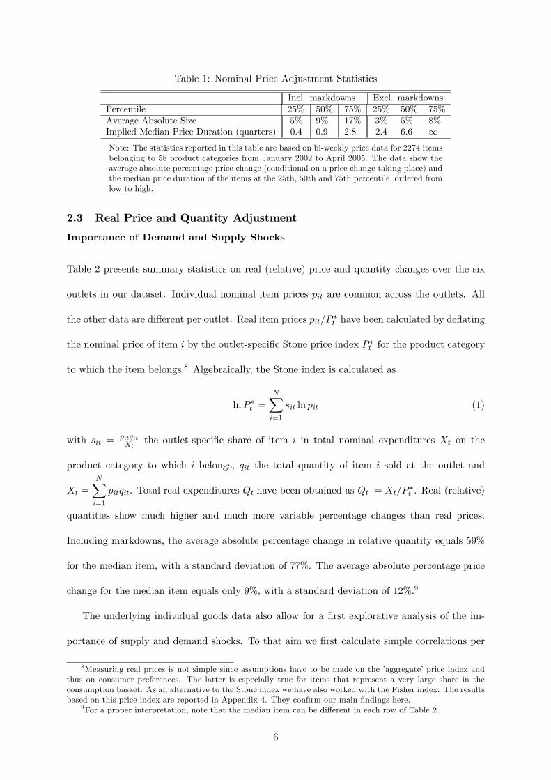
Table 1: Nominal Price Adjustment Statistics
Incl. markdowns Excl. markdownsPercentile 25% 50% 75% 25% 50% 75%Average Absolute Size 5% 9% 17% 3% 5% 8%Implied Median Price Duration (quarters) 0.4 0.9 2.8 2.4 6.6 1Note: The statistics reported in this table are based on bi-weekly price data for 2274 itemsbelonging to 58 product categories from January 2002 to April 2005. The data show theaverage absolute percentage price change (conditional on a price change taking place) andthe median price duration of the items at the 25th, 50th and 75th percentile, ordered fromlow to high.
2.3 Real Price and Quantity Adjustment
Importance of Demand and Supply Shocks
Table 2 presents summary statistics on real (relative) price and quantity changes over the six
outlets in our dataset. Individual nominal item prices pit are common across the outlets. All
the other data are di¤erent per outlet. Real item prices pit=P �t have been calculated by de�ating
the nominal price of item i by the outlet-speci�c Stone price index P �t for the product category
to which the item belongs.8 Algebraically, the Stone index is calculated as
lnP �t =NXi=1
sit ln pit (1)
with sit =pitqitXt
the outlet-speci�c share of item i in total nominal expenditures Xt on the
product category to which i belongs, qit the total quantity of item i sold at the outlet and
Xt =
NXi=1
pitqit. Total real expenditures Qt have been obtained as Qt = Xt=P �t . Real (relative)
quantities show much higher and much more variable percentage changes than real prices.
Including markdowns, the average absolute percentage change in relative quantity equals 59%
for the median item, with a standard deviation of 77%. The average absolute percentage price
change for the median item equals only 9%, with a standard deviation of 12%.9
The underlying individual goods data also allow for a �rst explorative analysis of the im-
portance of supply and demand shocks. To that aim we �rst calculate simple correlations per
8Measuring real prices is not simple since assumptions have to be made on the �aggregate�price index andthus on consumer preferences. The latter is especially true for items that represent a very large share in theconsumption basket. As an alternative to the Stone index we have also worked with the Fisher index. The resultsbased on this price index are reported in Appendix 4. They con�rm our main �ndings here.
9For a proper interpretation, note that the median item can be di¤erent in each row of Table 2.
6

item and per outlet between the change in real (relative) item prices and the change in relative
quantities sold. In case demand shocks dominate supply shocks, we should mainly �nd positive
correlations between items�price and quantity changes. In case supply shocks are dominant,
we should observe negative correlations. Next we split up the calculated variance in individ-
ual items�real price and quantity changes into a fraction due to supply shocks and a fraction
due to demand shocks. The bottom rows of Table 2 show the fractions due to supply shocks.
Concentrating on price changes, this fraction has been computed as
% Supply shocks to � ln(pit=P �t ) =
TXt=1;SS
(� ln(pit=P�t )� �i) 2
TXt=1
(� ln(pit=P �t )� �i) 2� 100
where �i is the mean of � ln(pit=P �t ) over all periods t. The numerator of this ratio includes
only observations where price and accompanying quantity changes in t have the opposite sign,
revealing a supply shock (SS). The denominator includes all observations. The fraction of the
variance in real price changes due to demand shocks, can be calculated as 1 minus the fraction
due to supply shocks. Our results reveal that price and quantity changes are mainly driven by
supply shocks. Including all data, the median item shows a clearly negative correlation between
price and quantity changes equal to -0.23. Moreover, about 65% of the variance in price and
quantity changes seems to follow from supply shocks.
The right part of Table 2 presents results obtained from data excluding markdown periods.
Temporary price markdowns are interesting supply shocks to identify a possibly kinked demand
curve, but we do not consider them as representing idiosyncratic supply shocks such as shifts
in costs or technology.10 We have therefore �ltered them out to gauge the importance of
idiosyncratic demand and supply shocks for markets where temporary price markdowns are
rare. As can be seen, the results at the right hand side of the table are fully in line with those
at the left hand side.10Note that we only exclude the item whose price is marked down, while keeping the other items. The e¤ects of
the (excluded) marked down item on the other items are thus not �ltered out. If we excluded all items in periodswhere at least one item in the product category is marked down, we would be left with almost no observations.
7

Table 2: Importance of Demand and Supply Shocks
Including markdowns Excl. markdownsPercentile 25% 50% 75% 25% 50% 75%Average absolute � ln(pit=P �t ) 6% 9% 15% 5% 8% 15%Average absolute � ln(qit=Qt) 39% 59% 80% 38% 59% 79%Standard Deviation � ln(pit=P �t ) 7% 12% 21% 7% 12% 21%Standard Deviation � ln(qit=Qt) 52% 77% 102% 51% 77% 101%Correlation (� ln(pit=P �t );� ln(qit=Qt)) -0.49 -0.23 0.02 -0.50 -0.24 0.01% Supply Shocks to � ln(pit=P �t )
(a) 48% 68% 86% 48% 69% 87%% Supply Shocks to � ln(qit=Qt) (a) 45% 64% 81% 45% 64% 82%
Note: The statistics reported in this table are based on bi-weekly data for 2274 itemsbelonging to 58 product categories in six outlets. Individual nominal item prices (pi) arecommon across the outlets, all the other data (P �; qi; Q) can be di¤erent per outlet. (a)The contribution of demand shocks to price and quantity variability equals 1 minus thecontribution of supply shocks. Computation methods are described in the main text.
An analysis of the relative importance of supply versus demand shocks is important for
more than one reason. First, this is important to know in order to do a proper econometric
demand analysis. One needs enough variation in supply to be able to identify a demand curve.
Our results in Table 2 are obviously encouraging in this respect. The minor contribution of
demand shocks should not be surprising given that prices are being set in advance or in the
very beginning of the period. As long as the supplier11 does not know demand in advance,
demand shocks cannot have an e¤ect on prices.12 Second, the results of a decomposition of the
variance of price changes into fractions due to demand and supply shocks may be important
for a proper calibration of theoretical macro models. In order to explain large price changes,
a number of authors have introduced idiosyncratic shocks in their models, a¤ecting prices and
quantities (Golosov and Lucas, 2003; Dotsey, King and Wolman, 2006; Klenow and Willis,
2006). As Klenow and Willis (2006) point out, there is not much empirical evidence available
that tells us whether these idiosyncratic shocks are mainly supply-driven or demand-driven.
Evidence like ours on the importance of demand and supply shocks excluding markdowns, as
11When we use the concept �supplier� we mean the retailer and the producer together. Usually prices inthe retail sector are set in an agreement between the retailer and the producer, so that there is not one easilyidenti�able party that sets prices.
12Of course, one could argue that the supplier does know in advance that demand will be high or low, so thathe can already at the moment of price setting �x an appropriate price. The data in Table 2, however, do notprovide strong evidence for this hypothesis. We come back to the risks that this alternative hypothesis mightimply for our econometric analysis in Section 3.
8

well as the extent of supply and demand shocks may be very indicative.13
Basic Evidence on Asymmetric Price Sensitivity
An explorative analysis of our data may also provide a �rst indication on the kinked demand
curve hypothesis that the price elasticity of demand rises in a product�s relative price. Figure 1
may be helpful to clarify our identi�cation. Per item we relate real (relative) prices to quantities
in natural logs. All relative price and quantity data have been demeaned to account for item
speci�c �xed e¤ects. The average is thus at the origin.
Figure 1: Identi�cation of Asymmetry in the DemandCurve
An important element is then to use supply shocks to identify the demand curve and po-
tential asymmetries in demand. We consider simultaneous increases or decreases in prices and
quantities as demand shocks, whereas we consider shifts in prices and quantities that go into
opposite directions as supply shocks. Our approach to identify the asymmetry in the demand
curve is to use only the price-quantity information that is consistent with movements along
the bold arrows. In particular, we use all couples of consecutive (log relative) price-quantity
observations that lie in the second or fourth quadrant and that re�ect a negative slope. Each
couple allows us to calculate a corresponding price elasticity as the inverse of this slope. Price-
quantity observations that do not respect this double condition (see the dotted arrows) are not
13This exercise is similar to the documentation of macroeconomic stylized facts in Cooley and Ohanian (1991)and Danthine and Donaldson (1993).
9
considered. For the latter changes it is less clear whether they took place along the (potentially)
low or high elasticity part of the demand curve. The last step is to compute the median of all
price elasticities that meet our conditions in the second quadrant, where the relative price is
high, and to repeat this in the fourth quadrant where the relative price is low.
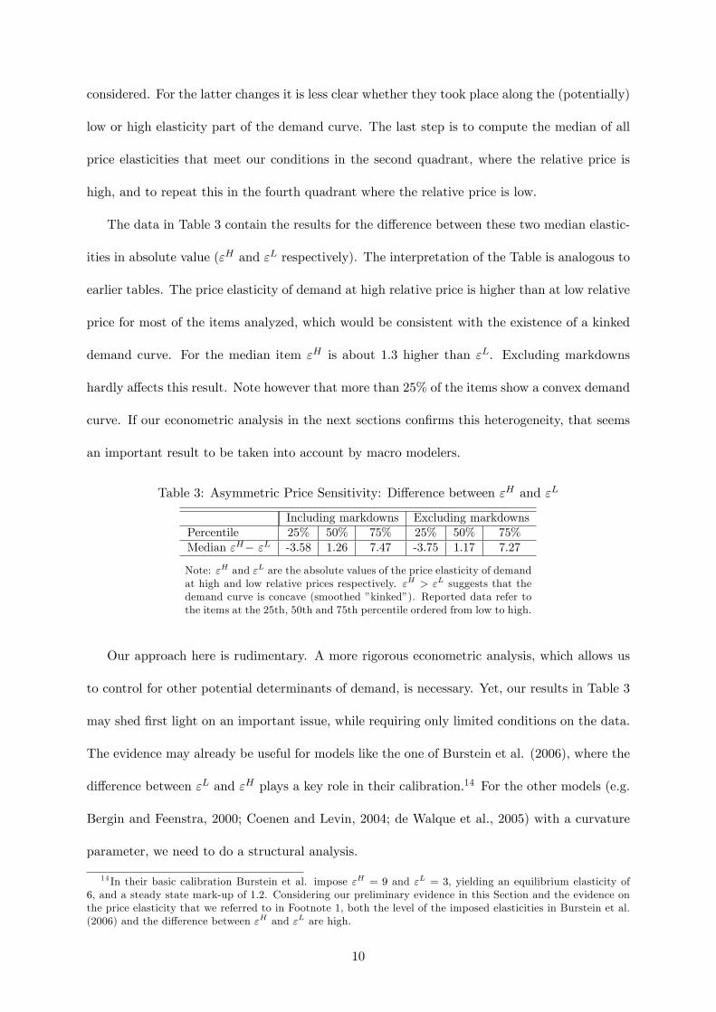
The data in Table 3 contain the results for the di¤erence between these two median elastic-
ities in absolute value ("H and "L respectively). The interpretation of the Table is analogous to
earlier tables. The price elasticity of demand at high relative price is higher than at low relative
price for most of the items analyzed, which would be consistent with the existence of a kinked
demand curve. For the median item "H is about 1.3 higher than "L. Excluding markdowns
hardly a¤ects this result. Note however that more than 25% of the items show a convex demand
curve. If our econometric analysis in the next sections con�rms this heterogeneity, that seems
an important result to be taken into account by macro modelers.
Table 3: Asymmetric Price Sensitivity: Di¤erence between "H and "L
Including markdowns Excluding markdownsPercentile 25% 50% 75% 25% 50% 75%Median "H� "L -3.58 1.26 7.47 -3.75 1.17 7.27
Note: "H and "L are the absolute values of the price elasticity of demandat high and low relative prices respectively. "H > "L suggests that thedemand curve is concave (smoothed �kinked�). Reported data refer tothe items at the 25th, 50th and 75th percentile ordered from low to high.
Our approach here is rudimentary. A more rigorous econometric analysis, which allows us
to control for other potential determinants of demand, is necessary. Yet, our results in Table 3
may shed �rst light on an important issue, while requiring only limited conditions on the data.
The evidence may already be useful for models like the one of Burstein et al. (2006), where the
di¤erence between "L and "H plays a key role in their calibration.14 For the other models (e.g.
Bergin and Feenstra, 2000; Coenen and Levin, 2004; de Walque et al., 2005) with a curvature
parameter, we need to do a structural analysis.
14 In their basic calibration Burstein et al. impose "H = 9 and "L = 3, yielding an equilibrium elasticity of6, and a steady state mark-up of 1.2. Considering our preliminary evidence in this Section and the evidence onthe price elasticity that we referred to in Footnote 1, both the level of the imposed elasticities in Burstein et al.(2006) and the di¤erence between "H and "L are high.
10

3 How Large is the Curvature? An Econometric Analysis
In this section we estimate the price elasticity and the curvature of demand for a broad range
of goods in our scanner dataset described above. We extend the Almost Ideal Demand System
(AIDS) developed by Deaton and Muellbauer (1980a, 1980b) by introducing assumptions drawn
from behavioral decision theory. Our �behavioral� AIDS model allows for a more general
curvature, which is necessary to answer our research question. The model still has the original
AIDS nested as a special case. For several reasons we believe the AIDS is the most appropriate
for our purposes: (i) it is �exible with respect to estimating own- and cross-price elasticities;
(ii) it is simple, transparent and easy to estimate, allowing us to deal with a very large number
of product categories; (iii) it is most appropriate in a setup like ours where consumers may buy
di¤erent items of given product categories; (iv) it is not necessary to specify the characteristics
of all goods, and use these in the regressions. The latter three characteristics particularly
distinguish the AIDS from alternative approaches like the mixed logit model used by Berry
et al. (1995). Their demand model is based on a discrete-choice assumption under which
consumers purchase at most one unit of one item of the di¤erentiated product. This assumption
is appropriate for large purchases such as cars. In a context where consumers might have a taste
for diversity and purchase several items, it may be less suitable. Moreover, to estimate Berry
et al. (1995)�s mixed logit model, the characteristics of all goods/items must be speci�ed. In
the case of cars this is a much easier task to do than for instance for cement or spaghetti.
Computational requirements of their methodology are also very demanding.
We follow the approach of Broda and Weinstein (2006) to cover as many goods as possible in
order to get a reliable estimate for the aggregate curvature, useful in calibrated macro models.
In Section 3.1 we �rst describe our extension of the AIDS model that should enable us to
answer our research question. Section 3.2 discusses our econometric setup and identi�cation
and estimation. Section 3.3 presents the results.
11

3.1 Model
Our extension of Deaton and Muellbauer�s AIDS model is speci�ed in expenditure share form
as
sit = �i +NXj=1
ij ln pjt + �i ln
�XtPt
�+
NXj=1
�ij
�ln(pjtPt)
�2(2)
for i = 1; :::; N and t = 1; :::; T . In this equation Xt is total nominal expenditure on the product
category of N items being analyzed (e.g. detergents), Pt is the price index for this product
category, pjt is the price of the jth item within the product category and sit is the share of total
expenditures allocated to item i (i.e. sit = pitqit=Xt). Deaton and Muellbauer de�ne the price
index Pt as
lnPt = �0 +
NXj=1
�j ln pjt +1
2
NXj=1
NXi=1
ij ln pit ln pjt (3)
Our extension of the model concerns the last term at the right hand side of Equation (2). The
original AIDS model has �ij = 0. Although this model is generally recognized to be �exible, it
is not �exible enough for our purposes. As we will demonstrate below, the curvature parameter,
which carries our main interest, is not free in the original AIDS model. It is a too restrictive
function of the price elasticity. This implies that in the original AIDS model it would not be
possible to obtain a convex demand curve empirically.
In extending the AIDS model we are inspired by relatively recent contributions to the the-
ory of consumer choice, which draw on behavioral decision theory and also have asymmetric
consumer reactions to price changes. Seminal work has been done by Kahneman, Tversky and
Thaler. An important idea in these contributions is that consumers evaluate choice alterna-
tives not only in absolute terms, but as deviations from a reference point (e.g. Tversky and
Kahneman, 1991). A popular representation of this idea is that consumers form a reference
price, with deviations between the actual price and the reference price conveying utility, and
thus in�uencing consumer purchasing behavior for a given budget constraint (see Putler, 1992).
We translate this idea to the context of standard macro models where consumers base their
12

decisions on the price of individual goods relative to the aggregate price, as in Dixit and Stiglitz
(1977) or Kimball (1995). The aggregate price would thus be the reference price. Within this
broader approach, consumers will not only buy less of a good when its price rises above the
aggregate price due to standard substitution and income e¤ects, but also because the price
rise may provoke negative feelings (utility losses). The consumer may for example feel being
treated unfairly, like in Okun (1981) or Rotemberg (2002). Inversely, the consumer will buy
more of a good for given actual prices and income when the actual price is below the aggregate.
Experiencing a relatively low price may in itself provoke a utility gain.
Figure 2 illustrates this argument. A key element is that the slope of an indi¤erence curve
through a single point in a good 1 and good 2 space will depend on whether the actual price
is relatively high or low compared to the relevant aggregate (reference) price. Initial prices of
goods 1 and 2 are pa1 and pa2. Both are equal to the aggregate price. The consumer maximizes
utility when she buys qa1 (point a). Then assume a price increase for good 1 to pb1, rotating the
budget line downwards. Traditional income and substitution e¤ects will make the consumer
move to point b, reducing the quantity of good 1 to qb1. Additional relative (or reference)
price e¤ects, however, will now shift the indi¤erence surface. With p1 now relatively high, the
indi¤erence curve through point b will become �atter. Intuitively, since buying good 1 conveys
utility losses, the consumer is willing to give up less of good 2 for more of good 1. The marginal
rate of substitution falls. The consumer reaches a new optimum at point d. Relative price
e¤ects on utility therefore induce an additional drop in q1 to qd1 . Note that a similar graphical
experiment can be done for a fall in p1. Tversky and Kahneman�s (1991) loss aversion hypothesis
would then predict opposite, but smaller relative price e¤ects, implying a kink in the demand
curve (see also Putler, 1992).
The implication of this argument is that relative price e¤ects on utility and the indi¤erence
surface should be accounted for in demand analysis. The added termNXj=1
�ij
�ln(
pjtPt)�2
in
Equation (2) allows us to capture these additional e¤ects. Provided that standard adding up
13
(NXi=1
�i = 1,NXi=1
ij = 0,NXi=1
�i = 0,NXi=1
�ij = 0), homogeneity (NXj=1
ij = 0) and symmetry
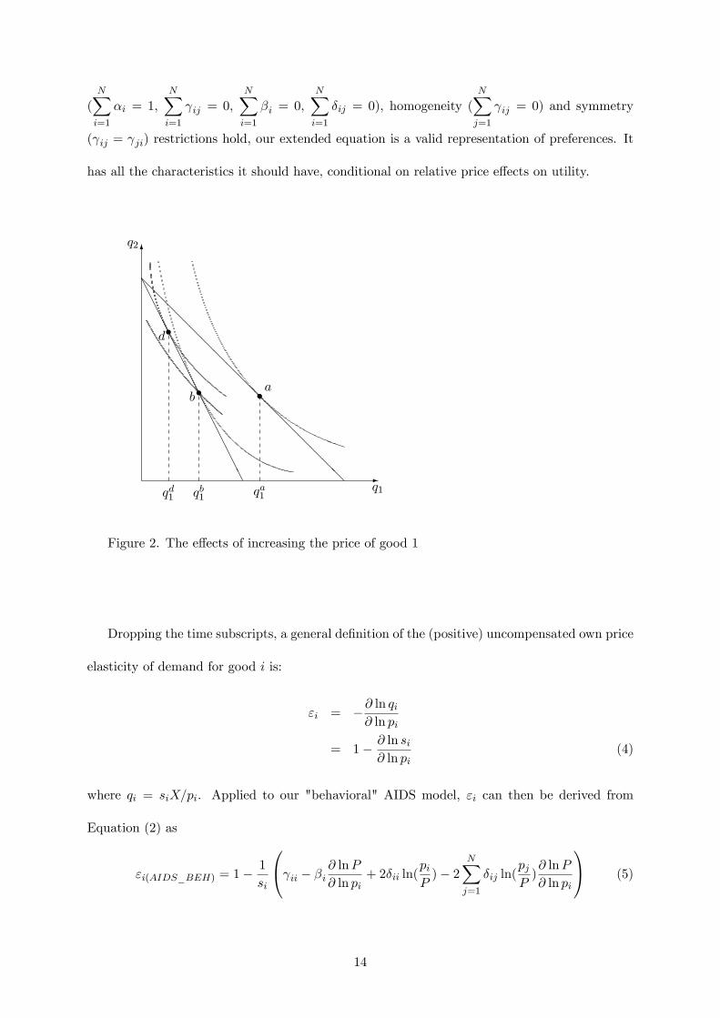
( ij = ji) restrictions hold, our extended equation is a valid representation of preferences. It
has all the characteristics it should have, conditional on relative price e¤ects on utility.
6
-q1
q2
qd1 qb1 qa1
@@@@@@@@@@@@@@@@@
AAAAAAAAAAAAAAAAA
ss sab
d
Figure 2. The e¤ects of increasing the price of good 1
Dropping the time subscripts, a general de�nition of the (positive) uncompensated own price
elasticity of demand for good i is:
"i = �@ ln qi@ ln pi
= 1� @ ln si@ ln pi
(4)
where qi = siX=pi. Applied to our "behavioral" AIDS model, "i can then be derived from
Equation (2) as
"i(AIDS_BEH) = 1�1
si
0@ ii � �i @ lnP@ ln pi+ 2�ii ln(
piP)� 2
NXj=1
�ij ln(pjP)@ lnP
@ ln pi
1A (5)
14
where we hold total nominal expenditure on the product category X as well as all other prices
pj (j 6= i) constant. In the AIDS model the correct expression for the elasticity of the group
price P with respect to pi is
@ lnP
@ ln pi= �i +
NXj=1
ij ln pj (6)
However, since using the price index from Equation (3) often raises empirical di¢ culties (see
e.g. Buse, 1994), researchers commonly use Stone�s geometric price index P � instead of P (see
Equation (1)). In our empirical work we will use Stone�s price index as well. The model is then
called the (extended) �linear approximate AIDS�(LA/AIDS). To obtain the own price elasticity
for the LA/AIDS model, we have to start from Stone�s P � and derive
@ lnP �
@ ln pi= si +
NXj=1
sj ln pj@ ln sj@ ln pi
(7)
Green and Alston (1990) and Buse (1994) discuss several approaches to computing the LA/AIDS
price elasticities depending on the assumptions made with regard to @ ln sj@ ln pi
and therefore @ lnP�
@ ln pi.
A common approach is to assume @ ln sj@ ln pi= 0, such that @ lnP
�
@ ln pi= si. Monte Carlo simulations by
Alston et al. (1994) and Buse (1994) reveal that this approximation is superior to many others
(e.g. smaller estimation bias). We will therefore use it in our empirical work. The (positive)
uncompensated own price elasticity implied by this approach is
"i(LA=AIDS_BEH) = 1� iisi+ �i �
2�ii ln(piP � )
si+ 2
NXj=1
�ij ln(pjP �) (8)
Equation (8) incorporates several channels for the relative price of an item to a¤ect the
price elasticity of demand. The contribution of our behavioral extension of the AIDS model is
obvious given the prominence of �ii in this equation. Since si is typically far below 1, observing
�ii < 0 would imply that the demand curve is likely to be concave, with "i rising in the relative
price piP � . When �ii > 0, it is more likely to �nd convexity in the demand curve.
At steady state, for relative prices equal to 1, the price elasticity becomes
"i(LA=AIDS_BEH_ST ) = 1� iisi+ �i (9)
15
Finally, starting from Equation (8) we show in Appendix 5 that the implied curvature of
the demand function at steady state is
�i(LA=AIDS_BEH) =@ ln "i@ ln pi
(10)
=1
"i
0@("i � 1) ("i � 1� �i)� 2�ii(1� si)si+ 2(�ii � si
NXj=1
�ij)
1A (11)
Also in this equation the key role of �ii stands out. For given price elasticity, the lower �ii, the
higher the estimated curvature.
A simple comparison of the above results with the price elasticity and the curvature in the
basic LA/AIDS model underscores the importance of our extension. Putting �ii = �ij = 0, one
can derive for the basic LA/AIDS model that
"i(LA=AIDS) = 1� iisi+ �i (12)
�i(LA=AIDS) =("i � 1)("i � 1� �i)
"i(13)
With �i mostly close to zero (and zero on average) the curvature then becomes a restrictive and
rising function of the price elasticity, at least for " > 1. Moreover, positive price elasticities "
almost unavoidably imply positive curvatures, which excludes convex demand curves. In light
of our �ndings in Table 3 this seems too restrictive.
3.2 Identi�cation/Estimation
The sample that we use for estimation contains data for 28 product categories sold in each of
the six outlets (supermarkets). The selection of these 28 categories, coming from 58 in Section
2, is driven by data requirements and discussed in Appendix 2. The time frequency is a period
of two weeks, with the time series running from the �rst bi-week of 2002 until the 8th bi-week of
2005. To keep estimation manageable we include �ve items per product category. Four of these
items have been selected on the basis of clear criteria to improve data quality and estimation
capacity. The �fth item is called �other�. It is constructed as a weighted average of all other
items. We include �other� to fully capture substitution possibilities for the four main items.
16
Specifying �other� also enables us to deal with entry and exit of individual items during the
sample period. We discuss the selection of the four items and the construction of �other� in
Appendix 2 as well. For each item i within a product category the basic empirical demand
speci�cation is:
simt = �im +
5Xj=1
ij ln pjt + �i ln
�XmtP �mt
�+
5Xj=1
�ij
�ln(
pjtP �mt
)
�2+
5Xj=1
'ijCjt + �it + "imt
i = 1; ::::; 5 m = 1; ::::; 6 t = 1; ::::; 86 (14)
where simt is the share of item i in total product category expenditure at outlet m and time
t, Xmt is overall product category expenditure at outlet m, P �mt is Stone�s price index for the
category at outlet m and pjt is the price of the jth item in the category. As we have mentioned
before, individual item prices are equal across outlets15 and predetermined. They are not
changed during the period. This is an important characteristic of our data, which strongly
facilitates identi�cation of the demand curve (cf. supra). Furthermore, �im captures item
speci�c and outlet speci�c �xed e¤ects. Finally, we include dummies to capture demand shocks
with respect to item i at time t which are common across outlets. Circular dummies Cjt are
equal to 1 when an item j in the product category to which i belongs, is mentioned in the
supermarket�s circular. The circular is common to all outlets. Also, for each item we include
three time dummies �it for New Year, Easter and Christmas. These dummies should capture
shifts in market share from one item to another during the respective periods.
Our estimation method is SUR. A key assumption underlying this choice is that prices pit
are uncorrelated with the error term "imt. For at least two reasons we believe this assumption
is justi�ed. Problems to identify the demand curve, as discussed by e.g. Hausman et al. (1994),
Hausman (1997) and Menezes-Filho (2005), should therefore not exist. First, since our retailer
sets prices in advance and does not change them to equilibrate supply and demand in a given
period, prices can be considered predetermined with respect to Equation (14). Second, prices
15The Stone index will di¤er per outlet due to di¤erent individual item weights.
17

are set equal for all six outlets.16 We assume that outlet speci�c demand shocks for an item do
not a¤ect the price of that item at the chain level. Of course, against these explanations one
could argue that the supplier may know in advance that demand will be high or low, so that
he can already at the moment of price setting �x an appropriate price. However, the results
in Table 2 do not provide strong evidence for this hypothesis. Demand shocks are of relatively
minor importance in driving price and quantity changes. Moreover, many demand shocks may
be captured by the circular dummies (Cjt) and the item speci�c time dummies (�it) included
in our equations. They will not show up in the error term. In the same vein, the included
�xed e¤ect �im captures the in�uence on expenditure shares of time-invariant product speci�c
characteristics which may also a¤ect the price charged by the retailer. Therefore, item speci�c
characteristics will not show up in the error term of the regressions either.
A robustness test that we discuss in the next section provides additional support for our
assumption that prices pit are uncorrelated with the error term "imt. Using IV methods we
obtain very similar results as the ones reported below.
Following Hausman et al. (1994) we estimate Equation (14) imposing homogeneity and
symmetry from the outset (i.e.5Xj=1
ij = 0 and ij = ji). We also impose symmetry on the
e¤ects of the circular dummies (i.e. 'ij = 'ji). Finally, note that the adding up conditions
(5Xi=1
�im = 1;
5Xi=1
ij = 0,5Xi=1
�i = 0,5Xi=1
�ij = 0) allow us to drop one equation from the
system. We drop the equation for "other".
3.3 Results
Estimation of Equation (14) for 28 product categories over six outlets, with each product cate-
gory containing four items, generates 672 estimated elasticities and curvatures. Since 6 of these
elasticities were implausible, we decided to drop them, leaving 666 plausible estimates.17
16The data used by e.g. Hausman et al., (1994), Hausman (1997) and Menezes-Filho (2005) do not have thischaracteristic.
17These 6 price elasticities were lower than -10 (where our de�nition is such that the elasticity for a negativelysloped demand curve should be a positive number). Note that we do not include the estimated elasticities andcurvatures for the composite �other�item in our further discussion. Due to the continuously changing compositionof this �other� item over time, any interpretation of the estimates would be delicate.
18

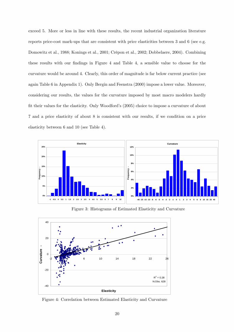
First, as we cannot discuss explicitly the 666 estimated elasticities and curvatures, we present
our results in the form of a histogram in Figure 3. We �nd that the unweighted median
price elasticity is 1.4. The unweighted median curvature is 0.8. If we weight our results with
the turnover each item generates, we do not �nd very di¤erent results. We �nd a median
weighted elasticity of 1.2 and a median weighted curvature of 0.8. Considering the values that
general equilibrium modelers impose when calibrating their models, these are low numbers (see
Table 6 in Appendix 1). The elasticities that we �nd are also low in comparison with the
existing empirical literature (see Bijmolt et al., 2005). The main reason for our relatively low
price elasticity seems to be the overrepresentation of necessities (e.g. corn�akes, baking �ower,
mineral water) in the product categories that we could draw from our dataset. The estimated
price elasticities for luxury goods, durables and large ticket items (e.g. smoked salmon, wine,
airing cupboards) are generally much higher.
Figure 4 and Table 4 bring more structure in our estimation results. Excluding some extreme
values for the curvature, Figure 4 reveals that the estimated price elasticity and curvature are
strongly positively correlated. The correlation coe¢ cient is 0.53.18 In Table 4 we report the
unweighted median elasticity and curvature, and their correlation, conditional on the elasticity
taking certain values. The condition that the elasticity is strictly higher than 1 corresponds to
the approach in standard macroeconomic models. When we impose this condition, the median
estimated price elasticity is 2.4, the median estimated curvature 1.7. Imposing that the elasticity
is strictly higher than 3 further raises the median curvature to 5.7. Estimated price elasticities
between 3 and 6 seem to go together with a median curvature of 3.5.
We can now reduce the uncertainty surrounding the curvature parameter to be used in
calibrated macro models. The empirical literature on the price elasticity of demand surveyed by
Bijmolt et al. (2005) reveals a median elasticity of about 2.2. Only 9% of estimated elasticities
18Figure 4 excludes 38 observations with an estimated curvature higher than 40 or lower than -40. If weexclude only observations with a curvature above +60 or below -60, the correlation is +0.51. Note that most ofthe extreme estimates for the curvature occur when the estimated price elasticity is very close to zero. Relativelysmall changes in the absolute value of the elasticity then result into, according to our de�nition of the curvature,huge percentage changes in the elasticity.
19
exceed 5. More or less in line with these results, the recent industrial organization literature
reports price-cost mark-ups that are consistent with price elasticities between 3 and 6 (see e.g.
Domowitz et al., 1988; Konings et al., 2001; Crépon et al., 2002; Dobbelaere, 2004). Combining
these results with our �ndings in Figure 4 and Table 4, a sensible value to choose for the
curvature would be around 4. Clearly, this order of magnitude is far below current practice (see
again Table 6 in Appendix 1). Only Bergin and Feenstra (2000) impose a lower value. Moreover,
considering our results, the values for the curvature imposed by most macro modelers hardly
�t their values for the elasticity. Only Woodford�s (2005) choice to impose a curvature of about
7 and a price elasticity of about 8 is consistent with our results, if we condition on a price
elasticity between 6 and 10 (see Table 4).
Elasticity
0%
5%
10%
15%
20%
25%
1 2 3 4 5 6 7 8 9 10 11 12 13 14 15 16 17 18 19 20
Freq
uenc
y
1 0.5 0 0.5 1 1.5 2 2.5 3 3.5 4 4.5 5 5.5 6 7 8 9 10
Curvature
0%
2%
4%
6%
8%
10%
12%
1 2 3 4 5 6 7 8 9 10 11 12 13 14 15 16 17 18 19 20 21 22 23 24
Freq
uenc
y
40 25 15 10 8 6 5 4 3 2 1 0 1 2 3 4 5 6 8 10 15 25 40
Figure 3: Histograms of Estimated Elasticity and Curvature
R2 = 0.28N.Obs. 628
40
20
0
20
40
2 2 6 10 14 18 22 26
Elasticity
Curv
atur
e
Figure 4: Correlation between Estimated Elasticity and Curvature
20
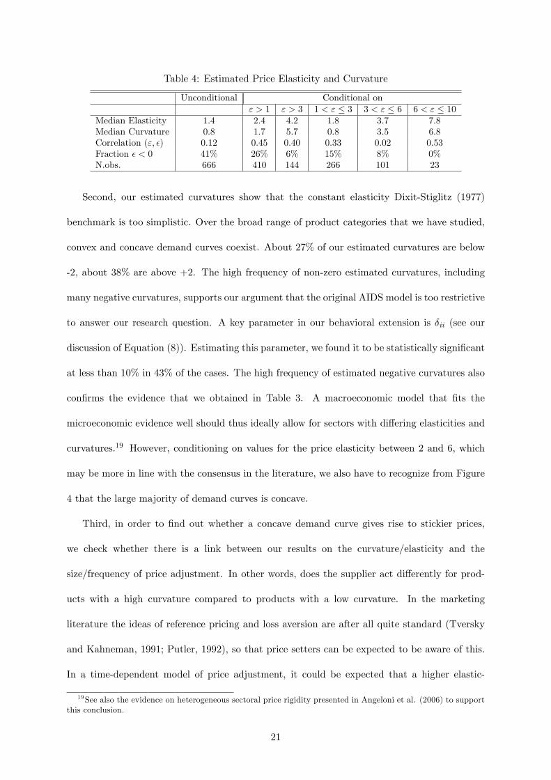
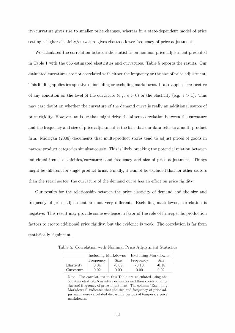
Table 4: Estimated Price Elasticity and Curvature
Unconditional Conditional on" > 1 " > 3 1 < " � 3 3 < " � 6 6 < " � 10
Median Elasticity 1.4 2.4 4.2 1.8 3.7 7.8Median Curvature 0.8 1.7 5.7 0.8 3.5 6.8Correlation ("; �) 0.12 0.45 0.40 0.33 0.02 0.53Fraction � < 0 41% 26% 6% 15% 8% 0%N.obs. 666 410 144 266 101 23
Second, our estimated curvatures show that the constant elasticity Dixit-Stiglitz (1977)
benchmark is too simplistic. Over the broad range of product categories that we have studied,
convex and concave demand curves coexist. About 27% of our estimated curvatures are below
-2, about 38% are above +2. The high frequency of non-zero estimated curvatures, including
many negative curvatures, supports our argument that the original AIDS model is too restrictive
to answer our research question. A key parameter in our behavioral extension is �ii (see our
discussion of Equation (8)). Estimating this parameter, we found it to be statistically signi�cant
at less than 10% in 43% of the cases. The high frequency of estimated negative curvatures also
con�rms the evidence that we obtained in Table 3. A macroeconomic model that �ts the
microeconomic evidence well should thus ideally allow for sectors with di¤ering elasticities and
curvatures.19 However, conditioning on values for the price elasticity between 2 and 6, which
may be more in line with the consensus in the literature, we also have to recognize from Figure
4 that the large majority of demand curves is concave.
Third, in order to �nd out whether a concave demand curve gives rise to stickier prices,
we check whether there is a link between our results on the curvature/elasticity and the
size/frequency of price adjustment. In other words, does the supplier act di¤erently for prod-
ucts with a high curvature compared to products with a low curvature. In the marketing
literature the ideas of reference pricing and loss aversion are after all quite standard (Tversky
and Kahneman, 1991; Putler, 1992), so that price setters can be expected to be aware of this.
In a time-dependent model of price adjustment, it could be expected that a higher elastic-
19See also the evidence on heterogeneous sectoral price rigidity presented in Angeloni et al. (2006) to supportthis conclusion.
21
ity/curvature gives rise to smaller price changes, whereas in a state-dependent model of price
setting a higher elasticity/curvature gives rise to a lower frequency of price adjustment.
We calculated the correlation between the statistics on nominal price adjustment presented
in Table 1 with the 666 estimated elasticities and curvatures. Table 5 reports the results. Our
estimated curvatures are not correlated with either the frequency or the size of price adjustment.
This �nding applies irrespective of including or excluding markdowns. It also applies irrespective
of any condition on the level of the curvature (e.g. � > 0) or the elasticity (e.g. " > 1). This
may cast doubt on whether the curvature of the demand curve is really an additional source of
price rigidity. However, an issue that might drive the absent correlation between the curvature
and the frequency and size of price adjustment is the fact that our data refer to a multi-product
�rm. Midrigan (2006) documents that multi-product stores tend to adjust prices of goods in
narrow product categories simultaneously. This is likely breaking the potential relation between
individual items� elasticities/curvatures and frequency and size of price adjustment. Things
might be di¤erent for single product �rms. Finally, it cannot be excluded that for other sectors
than the retail sector, the curvature of the demand curve has an e¤ect on price rigidity.
Our results for the relationship between the price elasticity of demand and the size and
frequency of price adjustment are not very di¤erent. Excluding markdowns, correlation is
negative. This result may provide some evidence in favor of the role of �rm-speci�c production
factors to create additional price rigidity, but the evidence is weak. The correlation is far from
statistically signi�cant.
Table 5: Correlation with Nominal Price Adjustment Statistics
Including Markdowns Excluding MarkdownsFrequency Size Frequency Size
Elasticity 0.04 -0.09 -0.10 -0.15Curvature 0.02 0.00 0.00 0.02
Note: The correlations in this Table are calculated using the666 item elasticity/curvature estimates and their correspondingsize and frequency of price adjustment. The column �ExcludingMarkdowns� indicates that the size and frequency of price ad-justment were calculated discarding periods of temporary pricemarkdowns.
22

We have tested the robustness of our estimation results in four ways. First, we have changed
the estimation methodology. A key assumption underlying the use of SUR is that prices pit
in Equation (14) are uncorrelated to the error term "imt. Although we believe we have good
reasons to make this assumption, we have dropped it as a robustness check, and re-estimated
our model using an IV method. Ideally, one can use information on costs, e.g. material prices,
as instruments. However, data on a su¢ cient number of input prices with a high enough
frequency is generally not available. Hausman et al. (1994) and Hausman (1997), who also use
prices and quantities in di¤erent outlets, solve this problem by exploiting the panel structure
of their data. They make the identifying assumption that prices in all outlets are driven by
common cost changes which are themselves independent of outlet speci�c variables. Prices in
other outlets then provide reliable instruments for the price in a speci�c outlet. This procedure
cannot work in our setup however since prices are identical across outlets. As an alternative we
have used once to three times lagged prices pi and once lagged relative pricespiP � as instruments.
Re-estimating our model for a large subset of the included product categories with the 3SLS
methodology, we obtained very similar results for the elasticities and curvatures.
As a second robustness check we have introduced seasonal dummies to capture possible
demand shifts related to the time of the year. As we have mentioned before, when suppliers are
aware of such demand shifts they may �x their price di¤erently. Not accounting for these demand
shifts may then introduce correlation between the price and the error term, and undermine the
quality of our estimates. Re-estimating our model with additional seasonal dummies did not
a¤ect our results in any serious way either.
Third, we allowed for gradual demand adjustment to price changes by adding a lagged
dependent variable to the regression. Although often statistically signi�cant, we generally found
the estimated parameter on this lagged dependent variable to be between +0.1 and -0.1. Gradual
adjustment seems to be no important issue in our dataset. Finally, our results are based on
the assumption that the aggregate price (P �t ) is the relevant reference price when consumers
23

make their choice. This assumption is in line with the approach in standard macro models.
In marketing literature however it is often assumed that reference prices are given at the time
of choice (see e.g. Putler, 1992; Bell and Latin, 2000). As a fourth robustness test we have
therefore assumed the reference price to be equal to the one-period lagged aggregate price P �t�1.
Re-estimating our model for a subset of product categories we found that this alternative had
no in�uence on the estimated price elasticities. It implied slightly higher estimated curvatures
for most items, however without a¤ecting any of our conclusions drawn above20.
4 Conclusions
The failure of nominal frictions to generate persistent e¤ects of monetary policy shocks has led
to the development of models which combine nominal and real price rigidities. Many researchers
have recently introduced a kinked (concave) demand curve as an attractive way to obtain real
rigidities. However, the literature su¤ers from a lack of empirical evidence on the existence of
the kinked demand curve and on the size of its curvature.
This paper uses scanner data from a large euro area retailer. Our main conclusions are
as follows. First, we �nd wide variation in the estimated price elasticity and the curvature of
demand among di¤erent products. Although demand for the median product is concave, the
fraction of products showing convex demand is signi�cant. Our �nding of wide heterogeneity,
with negative curvature for a large fraction of products, forms a challenge for the relevant
literature. It would suggest the need to model at least two sectors, one with real price �exibility,
and another with real price rigidity.
Second, our results support the introduction of a kinked (concave) demand curve in general
equilibrium macro models. We �nd that the price elasticity of demand is on average higher for
price increases than for price decreases. However, the degree of curvature in demand is much
lower than is currently imposed. Our suggestion would be to impose a curvature parameter
20Assuming that the reference price equals P �t�1 a¤ects the equation for the curvature. Instead of Equation(11) it then holds that �i = @ ln "i
@ ln pi= ("i�1)("i�1��i)�2�ii=si
"i.
24

around 4.
Third, we �nd no correlation between the estimated price elasticity/curvature and the ob-
served size or frequency of price adjustment in our data. Our speci�c context of a multi-product
retailer may however explain this lack of correlation.
Finding lower curvature than generally imposed, there must be other frictions at work, e.g.
frictions due to the introduction of �rm-speci�c marginal costs or a durable goods sector as in
Barsky et al. (2004). Or we need a combination with another reinforcing friction as in Bergin
and Feenstra (2000), who use the input-output structure of Basu (1995). After all, Bergin and
Feenstra (2000) do not need such a high curvature. Finally, there could also be other forms of
kinked demand (strategic complementarities) at work, but these are not testable with our data
and are probably not relevant in our economic environment. This kind of kink does not come
from consumer preferences, but must come from strategic interaction between suppliers.
References
[1] Alston J., Foster A. and R.Green, 1994, Estimating Elasticities with the Linear Approxi-
mate Almost Ideal Demand System: Some Monte Carlo Results, Review of Economics and
Statistics, 76, 351-356
[2] Altig D., Christiano L., Eichenbaum M. and J. Lindé, 2005, Firm-Speci�c Capital, Nominal
Rigidities and the Business Cycle, mimeo
[3] Angeloni I., Aucremanne L., Ehrmann M., Galí J., Levin A. and F. Smets, 2006, New
Evidence on In�ation Persistence and Price Stickiness in the Euro Area: Implications for
Macro Modelling, Journal of the European Economic Association, 4, 562-574
[4] Ball L. and D. Romer, 1990, Real Rigidities and the Non-Neutrality of Money, Review of
Economic Studies, 57, 183-203
25
[5] Barsky R., House C. and M. Kimball, 2004, Sticky Price Models and Durable Goods,
University of Michigan, mimeo
[6] Basu S., 1995, Intermediate Goods and Business Cycles: Implications for Productivity and
Welfare, American Economic Review, 85, 512-531
[7] Bell D.R. and J.R. Lattin, 2000, Looking for Loss Aversion in Scanner Panel Data: The
Confounding E¤ect of Price Response Heterogeneity, Marketing Science, 19, 185-200
[8] Bergin P. and R. Feenstra, 2000, Staggered Price Setting, Translog Preferences and En-
dogenous Persistence, Journal of Monetary Economics, 45, 657-680
[9] Berry S., Levinsohn J. and A. Pakes, 1995, Automobile Prices in Market Equilibrium,
Econometrica, 63, 841-890
[10] Bijmolt T., Van Heerde H. and R. Pieters, 2005, New empirical generalisations on the
determinants of price elasticity, Journal of Marketing Research, 42, 141-156
[11] Bils M. and P.J. Klenow, 2004, Some Evidence on the Importance of Sticky Prices, Journal
of Political Economy, 112, 947-985
[12] Blanchard O.J. and J. Galí, 2006, Real Wage Rigidities and the New Keynesian Model,
Journal of Money Credit and Banking, forthcoming
[13] Broda C. and D. Weinstein, 2006, Globalization and the Gains from Variety, Quarterly
Journal of Economics, 121, 541-585
[14] Burstein A., Eichenbaum M. and S. Rebelo, 2006, Modeling Exchange Rate Passthrough
after Large Devaluations, Journal of Monetary Economics, forthcoming
[15] Buse A., 1994, Evaluating the Linearized Almost Ideal Demand System, American Journal
of Agricultural Economics, 76, 781-793
26
[16] Calvo G., 1983, Staggered Prices in a Utility-Maximizing Framework, Journal of Monetary
Economics, 12, 383-398
[17] Chari V. Kehoe P. and E. McGrattan, 2000, Sticky Price Models of the Business Cycle:
Can the Contract Multiplier Solve the Persistence Problem, Econometrica, 68, 1151-1179
[18] Christiano L, Eichenbaum M. and C. Evans, 1999, Monetary Policy Shocks: What Have
We Learned and to What End?, Handbook of Macroeconomics,1A, eds, Michael Woodford
and John Taylor, Elsevier Science
[19] Christiano L., Eichenbaum M. and Evans C., 2005, Nominal Rigidities and the Dynamic
E¤ects of Shock to Monetary Policy, Journal of Political Economy, 113, 1-45
[20] Coenen G. and A. Levin, 2004, Identifying the in�uences of nominal and real rigidities in
aggregate price setting behavior, ECB Working Paper, No 418
[21] Cooley T. and L. Ohanian, 1991, The Cyclical Behavior of Prices, Journal of Monetary
Economics, 28, 25-60
[22] Crépon B., Desplatz R. and J. Mairesse, 2002, Price-Cost Margins and Rent Sharing:
Evidence from a Panel of French Manufacturing Firms, CREST, Centre de Recherche en
Economie et Statistique, Paris, mimeo
[23] Danthine J-P. and J. Donaldson, 1993, Methodological and Empirical Issues in Real Busi-
ness Cycle Theory, European Economic Review, 37, 1-35
[24] Deaton A. and J. Muellbauer, 1980a, An Almost Ideal Demand System, American Eco-
nomic Review, 70, 312-326
[25] Deaton A. and J. Muellbauer, 1980b, Economics of Consumer Behavior, Cambridge Uni-
versity Press
27
[26] de Walque G., Smets F. and R. Wouters, 2005, Firm-speci�c production factors in a DSGE
model with Taylor price setting, mimeo
[27] Dhyne E., Álvarez L., Le Bihan H., Veronese G., Dias D., Ho¤man J., Jonker N., Lünne-
mann P., Rumler F., and J. Vilmunen, 2006, Price setting in the euro area: Some stylized
facts from individual consumer price data, Journal of Economic Perspectives, 20, 171-192
[28] Dobbelaere S., 2004, Estimation of Price-Cost Margins and Union Bargaining Power for
Belgian Manufacturing, International Journal of Industrial Organization, 22, 1381-1398
[29] Domowitz I., Hubbard G. and B. Petersen, 1988, Market Structure and Cyclical Fluctua-
tions in US Manufacturing, Review of Economics and Statistics, 70, 55-66
[30] Dotsey M. and R. King, 2005, Implications of State-Dependent Pricing for Dynamic Macro-
economic Models, Journal of Monetary Economics, 52, 213-242
[31] Dotsey M., King R. and A. Wolman, 2006, In�ation and Real Activity with Firm-Level
Productivity Shocks: A Quantitative Framework, mimeo
[32] Dixit A. and J. Stiglitz, 1977, Monopolistic Competition and Optimum Product Diversity,
American Economic Review, 67, 297-308
[33] Eichenbaum M. and J. Fisher, 2004, Evaluating the Calvo Model of Sticky Prices, NBER
Working Paper, No 10617
[34] Galí J. and M. Gertler, 1999, In�ation Dynamics: A Structural Econometric Analysis,
Journal of Monetary Economics, 44, 195-222
[35] Golosov M. and R.E. Lucas Jr., 2003, Menu Costs and Phillips Curves, NBER Working
Paper, No 10187
[36] Green R and J. Alston, 1990, Elasticities in AIDS Models, American Journal of Agricultural
Economics, 72, 442-445
28
[37] Hausman J., 1997, Valuation of New Goods under Perfect and Imperfect Competition, in
The Economics of New Goods, Bresnahan and Gordon, eds., Chicago Press
[38] Hausman J., Leonard G. and J.D. Zona, 1994, Competitive Analysis with Di¤erentiated
Products, Annales d�Économie et de Statistique, 34, 159-180
[39] Kimball M., 1995, The Quantitative Analytics of the Basic Neomonetarist Model, Journal
of Money, Credit and Banking, 27, 1241-1277
[40] Klenow P.J. and O. Kryvtsov, 2005, State-Dependent or Time-Dependent Pricing: Does
It Matter for Recent U.S. In�ation?, mimeo
[41] Klenow P.J. and J.L. Willis, 2006, Real Rigidities and Nominal Price Changes, mimeo
[42] Konings J., Van Cayseele P. and F. Warzynski, 2001, The Dynamics of Industrial Mark-Ups
in Two Small Open Economies: Does National Competition Policy Matter? International
Journal of Industrial Organization, 19, 841-859
[43] Mankiw N.G., 1985, Small Menu Costs and Large Business Cycles, Quarterly Journal of
Economics, 100, 529-537
[44] Midrigan V., 2006, Menu Costs, Multi-Product Firms, and Aggregate Fluctuations, Ohio
State University, mimeo
[45] Menezes-Filho N., 2005, Is the Consumer Sector Competitive in the U.K.? A Test Using
Household-Level Demand Elasticities and Firm-Level Price Equations, Journal of Business
and Economic Statistics, 23, 295-304
[46] Okun A., 1981, Prices and Quantities, The Brookings Institution, Washington DC
[47] Peersman G., 2004, The Transmission of Monetary Policy in the Euro Area: Are the E¤ects
Di¤erent Across Countries?, Oxford Bulletin of Economics and Statistics, 66, 285-308
29

[48] Putler D.S., 1992, Incorporating Reference Price E¤ects into a Theory of Consumer Choice,
Marketing Science, 11, No 3, 287-309
[49] Rotemberg J., 2002, Customer Anger at Price Increases, Time Variation in the Frequency
of Price Changes and Monetary Policy, NBER Working Paper, No 9320
[50] Rotemberg J. and M. Woodford, 1999, The Cyclical Behavior of Prices and Costs, Handbook
of Macroeconomics, 1B, eds. J. Taylor and M. Woodford
[51] Sbordone A.M., 2002, Prices and Unit Labor Costs: A New Test of Price Stickiness, Journal
of Monetary Economics, 49, 265-292
[52] Taylor J., 1980, Aggregate Dynamics and Staggered Contracts, Journal of Political Econ-
omy, 88, 1-23
[53] Tversky A. and D. Kahneman, 1991, Loss Aversion in Riskless Choice : A Reference-
Dependent Model, Quarterly Journal of Economics, 106, 1039-1061
[54] Woodford M, 2003, Interest and Prices: Foundations of a Theory of Monetary Policy,
Princeton, Princeton University Press
[55] Woodford M., 2005, Firm-speci�c Capital and the New Keynesian Phillips Curve, Inter-
national Journal of Central Banking, 1, September, 1-46
30

Appendix 1: Di¤erent Curvatures
This appendix gives an overview of the di¤erent calibrations of the "kink" or curvature in the
demand curve, that are used in the literature on price setting. Because the curvature is not
de�ned homogeneously across the di¤erent papers, we �rst derive the relationships between
these de�nitions before we compare the parameter values that have been imposed. Table 6
summarizes these parameter values. We use the following notation: xi = qi=Q is �rm i�s
relative output, pi is its price, "(xi) is the (positive) price elasticity of demand, �(xi) ="(xi)"(xi)�1
is the �rm�s desired markup. Assuming an aggregate price level equal to 1, pi also indicates the
�rm�s relative price.
Coenen and Levin (2004) de�ne the curvature of the demand curve as the relative slope of
the price elasticity of demand around steady state:
� =
��@"(xi)
@xi
�xi=1
(15)
Eichenbaum and Fisher (2004) and de Walque et al. (2005) de�ne the curvature as the
elasticity of the price elasticity of demand with respect to the relative price at steady state:
� =
�@"(xi)
@pi
pi"(xi)
�xi=1
(16)
It can be shown that in steady state both approaches are identical:
@"(xi)
@pi
pi"(xi)
=@"(xi)
@pi
pi"(xi)
@xi@xi
xixi=@"(xi)
@xi
pixi
@xi@pi
xi"(xi)
= �@"(xi)@xi
"(xi)xi"(xi)
Evaluated at steady state (xi = 1), this is equal to �@"(xi)@xi
.
Kimball (1995) characterizes the curvature in the demand curve by the elasticity of the
�rm�s desired markup with respect to relative output at steady state, i.e.
� =
�@�(xi)
@xi
xi�(xi)
�xi=1
(17)
31
The relationship between � and � is as follows:
� =
�@�(xi)
@xi
xi�(xi)
�xi=1
=
��@�(xi)
@"(xi)
@pi@xi
xipi
"(xi)
�(xi)
�xi=1
=
��
1
("(xi)� 1)21
"(xi)("(xi)� 1)
�xi=1
=�
("(1)� 1) "(1)
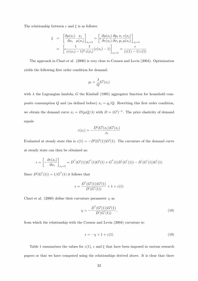
The approach in Chari et al. (2000) is very close to Coenen and Levin (2004). Optimization
yields the following �rst order condition for demand:
pi =�
QG0(xi)
with � the Lagrangian lambda, G the Kimball (1995) aggregator function for household com-
posite consumption Q and (as de�ned before) xi = qi=Q. Rewriting this �rst order condition,
we obtain the demand curve xi = D(piQ=�) with D = (G0)�1. The price elasticity of demand
equals
"(xi) = �D0(G0(xi))G0(xi)
xi
Evaluated at steady state this is "(1) = �D0(G0(1))G0(1). The curvature of the demand curve
at steady state can then be obtained as:
� =
��@"(xi)
@xi
�xi=1
= D00(G0(1))G
00(1)G0(1) +G
00(1)D
0(G
0(1))�D0
(G0(1))G
0(1)
Since D0(G0(1)) = 1=G
00(1) it follows that
� =D
00(G0(1))G0(1)
D0(G0(1))+ 1 + "(1)
Chari et al. (2000) de�ne their curvature parameter � as
� = �D00(G0(1))G0(1)
D0(G0(1)); (18)
from which the relationship with the Coenen and Levin (2004) curvature is:
� = ��+ 1 + "(1) (19)
Table 1 summarizes the values for "(1), � and � that have been imposed in various research
papers or that we have computed using the relationships derived above. It is clear that there
32
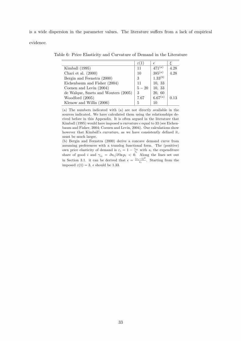
is a wide dispersion in the parameter values. The literature su¤ers from a lack of empirical
evidence.
Table 6: Price Elasticity and Curvature of Demand in the Literature
"(1) � �
Kimball (1995) 11 471(a) 4:28Chari et al. (2000) 10 385(a) 4:28Bergin and Feenstra (2000) 3 1:33(b)
Eichenbaum and Fisher (2004) 11 10; 33Coenen and Levin (2004) 5� 20 10; 33de Walque, Smets and Wouters (2005) 3 20; 60Woodford (2005) 7:67 6:67(a) 0:13Klenow and Willis (2006) 5 10
(a) The numbers indicated with (a) are not directly available in thesources indicated. We have calculated them using the relationships de-rived before in this Appendix. It is often argued in the literature thatKimball (1995) would have imposed a curvature � equal to 33 (see Eichen-baum and Fisher, 2004; Coenen and Levin, 2004). Our calculations showhowever that Kimball�s curvature, as we have consistently de�ned it,must be much larger.(b) Bergin and Feenstra (2000) derive a concave demand curve fromassuming preferences with a translog functional form. The (positive)own price elasticity of demand is "i = 1 � ii
siwith si the expenditure
share of good i and ii = @si=@ ln pi < 0. Along the lines set out
in Section 3.1. it can be derived that � = ("i�1)2"i
. Starting from theimposed "(1) = 3, � should be 1:33.
33

Appendix 2: Description of Dataset
Table 7 gives an overview of the 58 product categories that are in the dataset that we used
in this paper. Between brackets we indicate the number of items within each category. The
available data for all these categories have been used to compute the basic statistics in Section
2. Product categories in italic are also included in the econometric analysis in Section 3.
Table 7: Product Categories and Number of Items
Drinks: tea (67), coke (39), chocolate milk (9), lemonade (33), mineral water (66), wine (17)port wine (54), gin (21), fruit juice (54), beer (6), whiskey (82)Food: corn�akes (49), tuna (46), smoked salmon (18), biscuit (9), mayonnaise (45), tomatosoup (5), emmental cheese (56), gruyere cheese (19), spinach (29), margarine (62), potatoes (26),liver torta (98), baking �ower (18), spaghetti (30), co¤ee biscuits (5), minarine (2)Equipment: airing cupboard (61), knife (19), hedge shears (32), dishwasher (43), washingmachine (36), tape measure (15), tap (24), dvd recorder (20), casserole (74), toaster (40)Clothes and related: jeans (79), jacket (88)Cleaning products: dishwasher detergent (43), detergent (43), soap powder (98), �oorcloth (11)toilet soap (34)Leisure and education: hometrainer (52), football (32), cartoon (86), dictionary (32),school book (34)Personal care: plaster (33), nail polish (15), handkerchief (63), nappy (64), toilet paper (13)Other: potting soil (33), cement (43), bath mat (48), aluminium foil (5)
Note: The number of items in a particular product category is stated in brackets. Only the productcategories in italic are included in the econometric analysis in Section 3.
Our econometric analysis in Section 3 includes four items per product category and a com-
posite of all other items in the category, called �other�. Our criteria to select the four items
were (long) data availability and (relatively high) market share within the category.21 More
precisely, we ranked all products within the category on the basis of the total number of obser-
vations available (the maximum being 86), and chose those products with the highest number
of observations. Among items with an equal number of observations we selected those with
the highest market share. If this procedure implied di¤erent selections among the six available
outlets, we chose those products with the best ranking in most outlets.
The market share of �other�has been constructed as
sother;t =Xother;tXt
=
NXj =2S4
pjtqjt
Xt21Note that both these criteria are strongly (positively) correlated.
34

with S4 the selected four items, and all other variables as de�ned in the main text. The price
index of �other�is the Stone index for all items included in �other�.
pother;t =
NXj =2S4
sjtpjt
with sjt = pjtqjt=Xother;t. Due to di¤erent weights the price of �other�will di¤er across the six
outlets.
The reduction to 28 product categories in the econometric analysis in Section 3, coming from
58, has been driven by the following criteria. For a category to be included in the econometric
analysis we required (i) data availability in all six outlets, (ii) the four selected items to have
a total market share of at least 20% in their product category and (iii) the four selected items
to show su¢ cient price variation. Over the whole time span the four items together should
show at least 20 price changes of at least 5%, where we counted the typical V-pattern of a price
markdown as 1 price change. At least 3 of these price changes should be regular price changes.
35
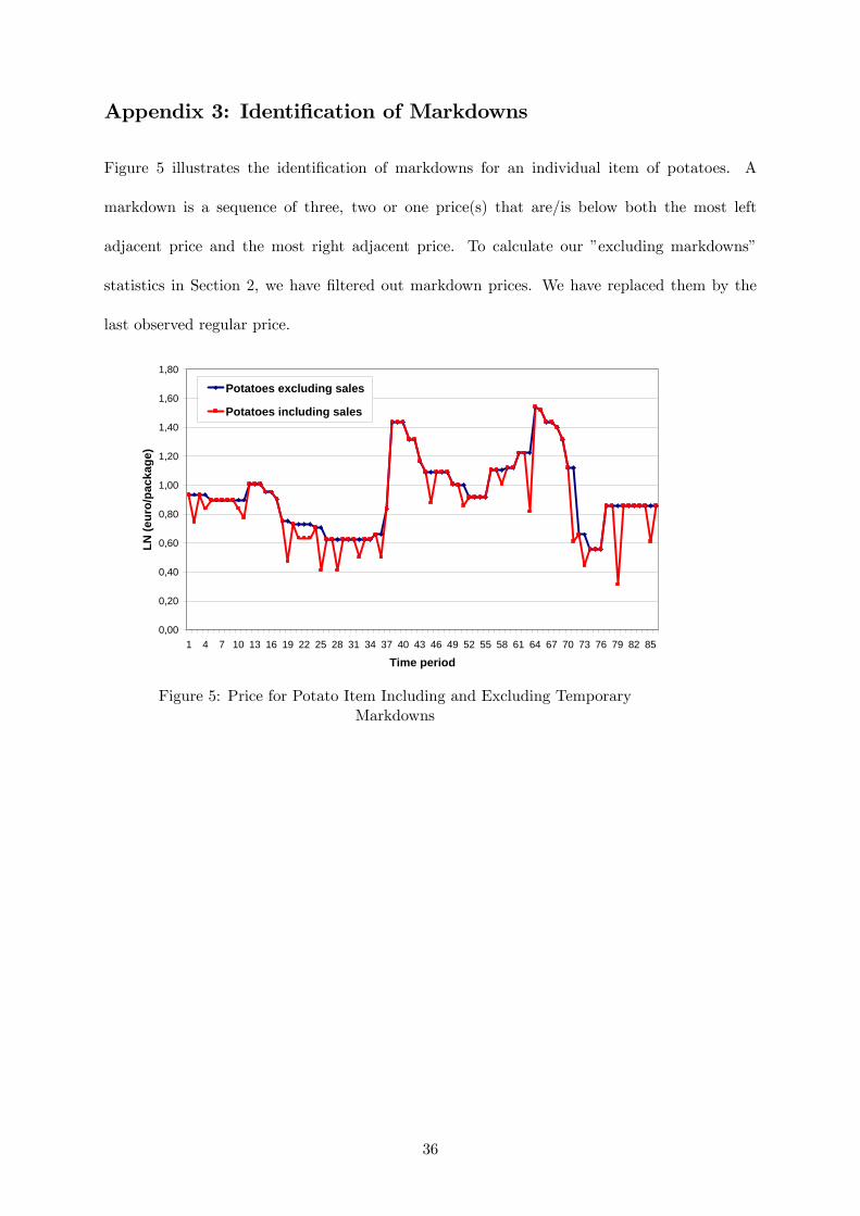
Appendix 3: Identi�cation of Markdowns
Figure 5 illustrates the identi�cation of markdowns for an individual item of potatoes. A
markdown is a sequence of three, two or one price(s) that are/is below both the most left
adjacent price and the most right adjacent price. To calculate our �excluding markdowns�
statistics in Section 2, we have �ltered out markdown prices. We have replaced them by the
last observed regular price.
0,00
0,20
0,40
0,60
0,80
1,00
1,20
1,40
1,60
1,80
1 4 7 10 13 16 19 22 25 28 31 34 37 40 43 46 49 52 55 58 61 64 67 70 73 76 79 82 85
Time period
LN (e
uro/
pack
age)
Potatoes excluding sales
Potatoes including sales
Figure 5: Price for Potato Item Including and Excluding TemporaryMarkdowns
36
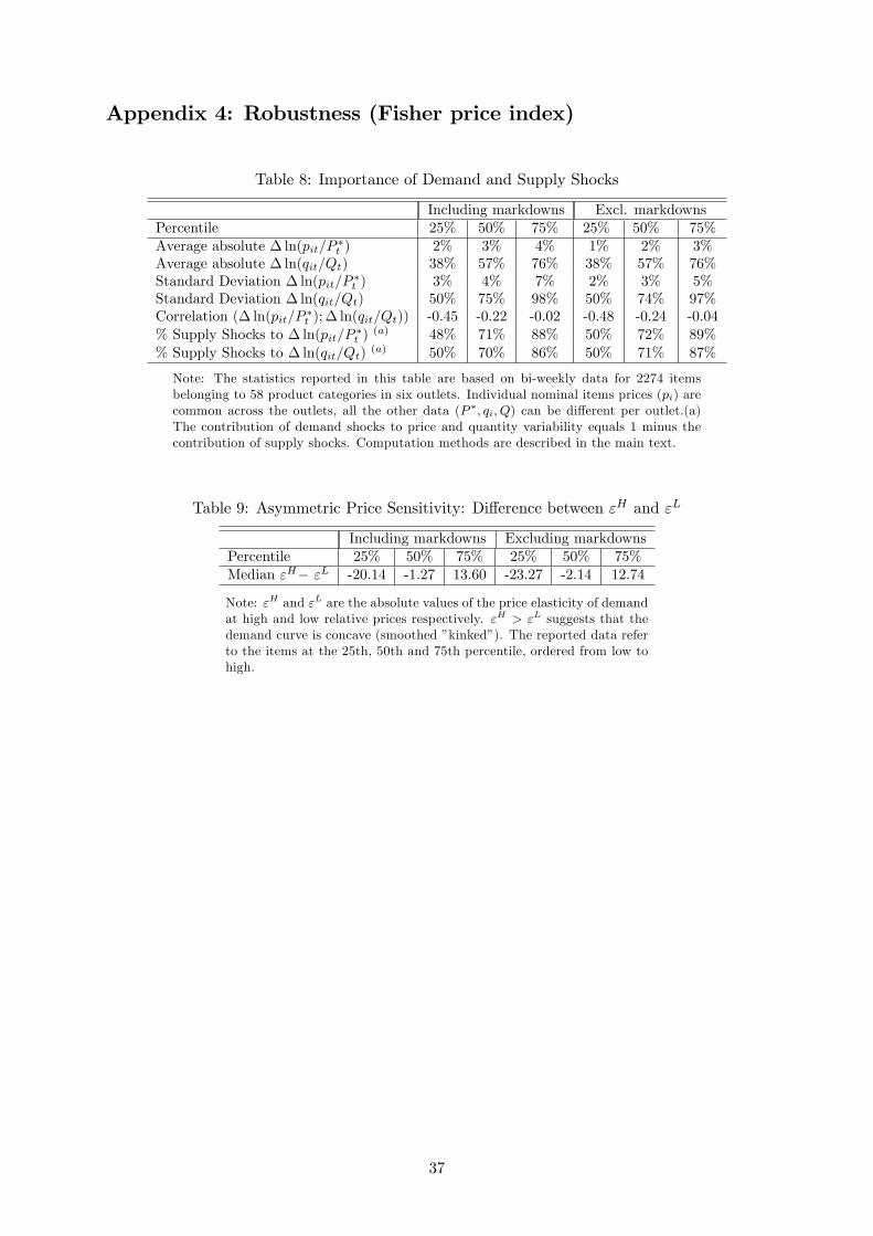
Appendix 4: Robustness (Fisher price index)
Table 8: Importance of Demand and Supply Shocks
Including markdowns Excl. markdownsPercentile 25% 50% 75% 25% 50% 75%Average absolute � ln(pit=P �t ) 2% 3% 4% 1% 2% 3%Average absolute � ln(qit=Qt) 38% 57% 76% 38% 57% 76%Standard Deviation � ln(pit=P �t ) 3% 4% 7% 2% 3% 5%Standard Deviation � ln(qit=Qt) 50% 75% 98% 50% 74% 97%Correlation (� ln(pit=P �t );� ln(qit=Qt)) -0.45 -0.22 -0.02 -0.48 -0.24 -0.04% Supply Shocks to � ln(pit=P �t )
(a) 48% 71% 88% 50% 72% 89%% Supply Shocks to � ln(qit=Qt) (a) 50% 70% 86% 50% 71% 87%
Note: The statistics reported in this table are based on bi-weekly data for 2274 itemsbelonging to 58 product categories in six outlets. Individual nominal items prices (pi) arecommon across the outlets, all the other data (P �; qi; Q) can be di¤erent per outlet.(a)The contribution of demand shocks to price and quantity variability equals 1 minus thecontribution of supply shocks. Computation methods are described in the main text.
Table 9: Asymmetric Price Sensitivity: Di¤erence between "H and "L
Including markdowns Excluding markdownsPercentile 25% 50% 75% 25% 50% 75%Median "H� "L -20.14 -1.27 13.60 -23.27 -2.14 12.74
Note: "H and "L are the absolute values of the price elasticity of demandat high and low relative prices respectively. "H > "L suggests that thedemand curve is concave (smoothed �kinked�). The reported data referto the items at the 25th, 50th and 75th percentile, ordered from low tohigh.
37
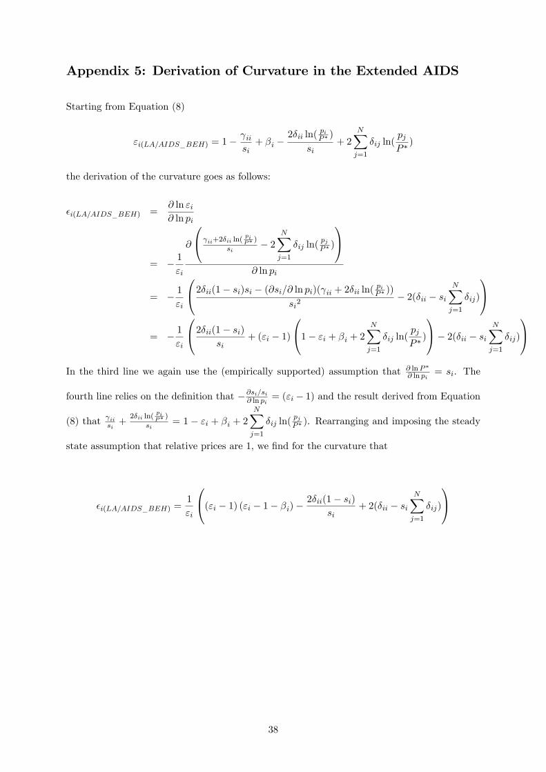
Appendix 5: Derivation of Curvature in the Extended AIDS
Starting from Equation (8)
"i(LA=AIDS_BEH) = 1� iisi+ �i �
2�ii ln(piP � )
si+ 2
NXj=1
�ij ln(pjP �)
the derivation of the curvature goes as follows:
�i(LA=AIDS_BEH) =@ ln "i@ ln pi
= � 1"i
@
0@ ii+2�ii ln(piP� )
si� 2
NXj=1
�ij ln(pjP � )
1A@ ln pi
= � 1"i
0@2�ii(1� si)si � (@si=@ ln pi)( ii + 2�ii ln( piP � ))si2
� 2(�ii � siNXj=1
�ij)
1A= � 1
"i
0@2�ii(1� si)si
+ ("i � 1)
0@1� "i + �i + 2 NXj=1
�ij ln(pjP �)
1A� 2(�ii � si NXj=1
�ij)
1AIn the third line we again use the (empirically supported) assumption that @ lnP �
@ ln pi= si. The
fourth line relies on the de�nition that �@si=si@ ln pi
= ("i � 1) and the result derived from Equation
(8) that iisi +2�ii ln(
piP� )
si= 1 � "i + �i + 2
NXj=1
�ij ln(pjP � ). Rearranging and imposing the steady
state assumption that relative prices are 1, we �nd for the curvature that
�i(LA=AIDS_BEH) =1
"i
0@("i � 1) ("i � 1� �i)� 2�ii(1� si)si+ 2(�ii � si
NXj=1
�ij)
1A
38

NBB WORKING PAPER No. 99 - OCTOBER 2006 39
NATIONAL BANK OF BELGIUM - WORKING PAPERS SERIES
1. "Model-based inflation forecasts and monetary policy rules" by M. Dombrecht and R. Wouters, ResearchSeries, February 2000.
2. "The use of robust estimators as measures of core inflation" by L. Aucremanne, Research Series,February 2000.
3. "Performances économiques des Etats-Unis dans les années nonante" by A. Nyssens, P. Butzen,P. Bisciari, Document Series, March 2000.
4. "A model with explicit expectations for Belgium" by P. Jeanfils, Research Series, March 2000.5. "Growth in an open economy: some recent developments" by S. Turnovsky, Research Series, May 2000.6. "Knowledge, technology and economic growth: an OECD perspective" by I. Visco, A. Bassanini,
S. Scarpetta, Research Series, May 2000.7. "Fiscal policy and growth in the context of European integration" by P. Masson, Research Series, May
2000.8. "Economic growth and the labour market: Europe's challenge" by C. Wyplosz, Research Series, May
2000.9. "The role of the exchange rate in economic growth: a euro-zone perspective" by R. MacDonald,
Research Series, May 2000.10. "Monetary union and economic growth" by J. Vickers, Research Series, May 2000.11. "Politique monétaire et prix des actifs: le cas des Etats-Unis" by Q. Wibaut, Document Series, August
2000.12. "The Belgian industrial confidence indicator: leading indicator of economic activity in the euro area?" by
J.-J. Vanhaelen, L. Dresse, J. De Mulder, Document Series, November 2000.13. "Le financement des entreprises par capital-risque" by C. Rigo, Document Series, February 2001.14. "La nouvelle économie" by P. Bisciari, Document Series, March 2001.15. "De kostprijs van bankkredieten" by A. Bruggeman and R. Wouters, Document Series, April 2001.16. "A guided tour of the world of rational expectations models and optimal policies" by Ph. Jeanfils,
Research Series, May 2001.17. "Attractive Prices and Euro - Rounding effects on inflation" by L. Aucremanne and D. Cornille,
Documents Series, November 2001.18. "The interest rate and credit channels in Belgium: an investigation with micro-level firm data" by
P. Butzen, C. Fuss and Ph. Vermeulen, Research series, December 2001.19 "Openness, imperfect exchange rate pass-through and monetary policy" by F. Smets and R. Wouters,
Research series, March 2002.20. "Inflation, relative prices and nominal rigidities" by L. Aucremanne, G. Brys, M. Hubert, P. J. Rousseeuw
and A. Struyf, Research series, April 2002.21. "Lifting the burden: fundamental tax reform and economic growth" by D. Jorgenson, Research series,
May 2002.22. "What do we know about investment under uncertainty?" by L. Trigeorgis, Research series, May 2002.23. "Investment, uncertainty and irreversibility: evidence from Belgian accounting data" by D. Cassimon,
P.-J. Engelen, H. Meersman, M. Van Wouwe, Research series, May 2002.24. "The impact of uncertainty on investment plans" by P. Butzen, C. Fuss, Ph. Vermeulen, Research series,
May 2002.25. "Investment, protection, ownership, and the cost of capital" by Ch. P. Himmelberg, R. G. Hubbard,
I. Love, Research series, May 2002.26. "Finance, uncertainty and investment: assessing the gains and losses of a generalised non-linear
structural approach using Belgian panel data", by M. Gérard, F. Verschueren, Research series,May 2002.
27. "Capital structure, firm liquidity and growth" by R. Anderson, Research series, May 2002.28. "Structural modelling of investment and financial constraints: where do we stand?" by J.- B. Chatelain,
Research series, May 2002.29. "Financing and investment interdependencies in unquoted Belgian companies: the role of venture
capital" by S. Manigart, K. Baeyens, I. Verschueren, Research series, May 2002.30. "Development path and capital structure of Belgian biotechnology firms" by V. Bastin, A. Corhay,
G. Hübner, P.-A. Michel, Research series, May 2002.31. "Governance as a source of managerial discipline" by J. Franks, Research series, May 2002.

40 NBB WORKING PAPER No. 99 - OCTOBER 2006
32. "Financing constraints, fixed capital and R&D investment decisions of Belgian firms" by M. Cincera,Research series, May 2002.
33. "Investment, R&D and liquidity constraints: a corporate governance approach to the Belgian evidence"by P. Van Cayseele, Research series, May 2002.
34. "On the Origins of the Franco-German EMU Controversies" by I. Maes, Research series, July 2002.35. "An estimated dynamic stochastic general equilibrium model of the Euro Area", by F. Smets and
R. Wouters, Research series, October 2002.36. "The labour market and fiscal impact of labour tax reductions: The case of reduction of employers' social
security contributions under a wage norm regime with automatic price indexing of wages", byK. Burggraeve and Ph. Du Caju, Research series, March 2003.
37. "Scope of asymmetries in the Euro Area", by S. Ide and Ph. Moës, Document series, March 2003.38. "De autonijverheid in België: Het belang van het toeleveringsnetwerk rond de assemblage van
personenauto's", by F. Coppens and G. van Gastel, Document series, June 2003.39. "La consommation privée en Belgique", by B. Eugène, Ph. Jeanfils and B. Robert, Document series,
June 2003.40. "The process of European monetary integration: a comparison of the Belgian and Italian approaches", by
I. Maes and L. Quaglia, Research series, August 2003.41. "Stock market valuation in the United States", by P. Bisciari, A. Durré and A. Nyssens, Document series,
November 2003.42. "Modeling the Term Structure of Interest Rates: Where Do We Stand?, by K. Maes, Research series,
February 2004.43. Interbank Exposures: An Empirical Examination of System Risk in the Belgian Banking System, by
H. Degryse and G. Nguyen, Research series, March 2004.44. "How Frequently do Prices change? Evidence Based on the Micro Data Underlying the Belgian CPI", by
L. Aucremanne and E. Dhyne, Research series, April 2004.45. "Firms' investment decisions in response to demand and price uncertainty", by C. Fuss and
Ph. Vermeulen, Research series, April 2004.46. "SMEs and Bank Lending Relationships: the Impact of Mergers", by H. Degryse, N. Masschelein and
J. Mitchell, Research series, May 2004.47. "The Determinants of Pass-Through of Market Conditions to Bank Retail Interest Rates in Belgium", by
F. De Graeve, O. De Jonghe and R. Vander Vennet, Research series, May 2004.48. "Sectoral vs. country diversification benefits and downside risk", by M. Emiris, Research series,
May 2004.49. "How does liquidity react to stress periods in a limit order market?", by H. Beltran, A. Durré and P. Giot,
Research series, May 2004.50. "Financial consolidation and liquidity: prudential regulation and/or competition policy?", by
P. Van Cayseele, Research series, May 2004.51. "Basel II and Operational Risk: Implications for risk measurement and management in the financial
sector", by A. Chapelle, Y. Crama, G. Hübner and J.-P. Peters, Research series, May 2004.52. "The Efficiency and Stability of Banks and Markets", by F. Allen, Research series, May 2004.53. "Does Financial Liberalization Spur Growth?" by G. Bekaert, C.R. Harvey and C. Lundblad, Research
series, May 2004.54. "Regulating Financial Conglomerates", by X. Freixas, G. Lóránth, A.D. Morrison and H.S. Shin, Research
series, May 2004.55. "Liquidity and Financial Market Stability", by M. O'Hara, Research series, May 2004.56. "Economisch belang van de Vlaamse zeehavens: verslag 2002", by F. Lagneaux, Document series,
June 2004.57. "Determinants of Euro Term Structure of Credit Spreads", by A. Van Landschoot, Research series,
July 2004.58. "Macroeconomic and Monetary Policy-Making at the European Commission, from the Rome Treaties to
the Hague Summit", by I. Maes, Research series, July 2004.59. "Liberalisation of Network Industries: Is Electricity an Exception to the Rule?", by F. Coppens and
D. Vivet, Document series, September 2004.60. "Forecasting with a Bayesian DSGE model: an application to the euro area", by F. Smets and
R. Wouters, Research series, September 2004.61. "Comparing shocks and frictions in US and Euro Area Business Cycle: a Bayesian DSGE approach", by
F. Smets and R. Wouters, Research series, October 2004.

NBB WORKING PAPER No. 99 - OCTOBER 2006 41
62. "Voting on Pensions: A Survey", by G. de Walque, Research series, October 2004.63. "Asymmetric Growth and Inflation Developments in the Acceding Countries: A New Assessment", by
S. Ide and P. Moës, Research series, October 2004.64. "Importance économique du Port Autonome de Liège: rapport 2002", by F. Lagneaux, Document series,
November 2004.65. "Price-setting behaviour in Belgium: what can be learned from an ad hoc survey", by L. Aucremanne and
M. Druant, Research series, March 2005.66. "Time-dependent versus State-dependent Pricing: A Panel Data Approach to the Determinants of
Belgian Consumer Price Changes", by L. Aucremanne and E. Dhyne, Research series, April 2005.67. "Indirect effects – A formal definition and degrees of dependency as an alternative to technical
coefficients", by F. Coppens, Research series, May 2005.68. "Noname – A new quarterly model for Belgium", by Ph. Jeanfils and K. Burggraeve, Research series,
May 2005.69. "Economic importance of the Flemish maritime ports: report 2003", F. Lagneaux, Document series, May
2005.70. "Measuring inflation persistence: a structural time series approach", M. Dossche and G. Everaert,
Research series, June 2005.71. "Financial intermediation theory and implications for the sources of value in structured finance markets",
J. Mitchell, Document series, July 2005.72. "Liquidity risk in securities settlement", J. Devriese and J. Mitchell, Research series, July 2005.73. "An international analysis of earnings, stock prices and bond yields", A. Durré and P. Giot, Research
series, September 2005.74. "Price setting in the euro area: Some stylized facts from Individual Consumer Price Data", E. Dhyne,
L. J. Álvarez, H. Le Bihan, G. Veronese, D. Dias, J. Hoffmann, N. Jonker, P. Lünnemann, F. Rumler andJ. Vilmunen, Research series, September 2005.
75. "Importance économique du Port Autonome de Liège: rapport 2003", by F. Lagneaux, Document series,October 2005.
76. "The pricing behaviour of firms in the euro area: new survey evidence, by S. Fabiani, M. Druant,I. Hernando, C. Kwapil, B. Landau, C. Loupias, F. Martins, T. Mathä, R. Sabbatini, H. Stahl andA. Stokman, Research series, November 2005.
77. "Income uncertainty and aggregate consumption, by L. Pozzi, Research series, November 2005.78. "Crédits aux particuliers - Analyse des données de la Centrale des Crédits aux Particuliers", by
H. De Doncker, Document series, January 2006.79. "Is there a difference between solicited and unsolicited bank ratings and, if so, why?" by P. Van Roy,
Research series, February 2006.80. "A generalised dynamic factor model for the Belgian economy - Useful business cycle indicators and
GDP growth forecasts", by Ch. Van Nieuwenhuyze, Research series, February 2006.81. "Réduction linéaire de cotisations patronales à la sécurité sociale et financement alternatif" by
Ph. Jeanfils, L. Van Meensel, Ph. Du Caju, Y. Saks, K. Buysse and K. Van Cauter, Document series,March 2006.
82. "The patterns and determinants of price setting in the Belgian industry" by D. Cornille and M. Dossche,Research series, May 2006.
83. "A multi-factor model for the valuation and risk management of demand deposits" by H. Dewachter,M. Lyrio and K. Maes, Research series, May 2006.
84. "The single European electricity market: A long road to convergence", by F. Coppens and D. Vivet,Document series, May 2006.
85. "Firm-specific production factors in a DSGE model with Taylor price setting", by G. de Walque, F. Smetsand R. Wouters, Research series, June 2006.
86. "Economic importance of the Belgian ports: Flemish maritime ports and Liège port complex - report2004", by F. Lagneaux, Document series, June 2006.
87. "The response of firms' investment and financing to adverse cash flow shocks: the role of bankrelationships", by C. Fuss and Ph. Vermeulen, Research series, July 2006.
88. "The term structure of interest rates in a DSGE model", by M. Emiris, Research series, July 2006.89. "The production function approach to the Belgian output gap, Estimation of a Multivariate Structural Time
Series Model", by Ph. Moës, Research series, September 2006.90. "Industry Wage Differentials, Unobserved Ability, and Rent-Sharing: Evidence from Matched Worker-
Firm Data, 1995-2002", by R. Plasman, F. Rycx and I. Tojerow, Research series, October 2006.

42 NBB WORKING PAPER No. 99 - OCTOBER 2006
91. "The dynamics of trade and competition", by N. Chen, J. Imbs and A. Scott, Research series, October2006.
92. "A New Keynesian Model with Unemployment", by O. Blanchard and J. Gali, Research series, October2006.
93. "Price and Wage Setting in an Integrating Europe: Firm Level Evidence", by F. Abraham, J. Konings andS. Vanormelingen, Research series, October 2006.
94. "Simulation, estimation and welfare implications of monetary policies in a 3-country NOEM model", byJ. Plasmans, T. Michalak and J. Fornero, Research series, October 2006.
95. "Inflation persistence and price-setting behaviour in the euro area: a summary of the Inflation PersistenceNetwork evidence ", by F. Altissimo, M. Ehrmann and F. Smets, Research series, October 2006.
96. "How Wages Change: Mirco Evidence from the International Wage Flexibility Project", by W.T. Dickens,L. Goette, E.L. Groshen, S. Holden, J. Messina, M.E. Schweitzer, J. Turunen and M. Ward, Researchseries, October 2006.
97. "Nominal wage rigidities in a new Keynesian model with frictional unemployment", by V. Bodart,G. de Walque, O. Pierrard, H.R. Sneessens and R. Wouters, Research series, October 2006.
98. "Dynamics on monetary policy in a fair wage model of the business cycle", by D. De la Croix,G. de Walque and R. Wouters, Research series, October 2006.
99. "The kinked demand curve and price rigidity: evidence from scanner data", by M. Dossche, F. Heylenand D. Van den Poel, Research series, October 2006.