working paper perceived precautionary savings motives
TRANSCRIPT

5757 S. University Ave.
Chicago, IL 60637
Main: 773.702.5599
bfi.uchicago.edu
WORKING PAPER · NO. 2019-140
Perceived Precautionary Savings Motives: Evidence from FinTechFrancesco D’Acunto, Thomas Rauter, Christoph Scheuch, and Michael WeberDECEMBER 2019

Perceived Precautionary Savings Motives:
Evidence from FinTech∗
Francesco D’Acunto Thomas Rauter
Christoph Scheuch Michael Weber
December 4, 2019
AbstractWe study the consumption response to the provision of credit lines to individuals thatpreviously did not have access to credit combined with the possibility to elicit directlya large set of preferences, beliefs, and motives. As expected, users react to the avail-ability of credit by increasing their spending permanently and reallocating consumptionfrom non-discretionary to discretionary goods and services. Surprisingly, though, liquidusers react more than others and this pattern is a robust feature of the data. More-over, liquid users lower their savings rate, but do not tap into negative deposits. Thecredit line seems to act as a form of insurance against future negative shocks and itsmere presence makes users spend their existing liquidity without accumulating any debt.By eliciting preferences, beliefs, and motives directly, we show these results are not fullyconsistent with models of financial constraints, buffer stock models with and withoutdurables, present-bias preferences, uncertainty about future income, bequest motives, orthe canonical life-cycle permanent income model. We label this channel the perceivedprecautionary savings channel, because liquid households behave as if they faced strongprecautionary savings motives even though no observables suggest they should based onstandard theoretical models.
JEL Codes: D14, E21, E51, G21Keywords: Household Finance, Consumption, Behavioral Finance
∗D’Acunto is at Boston College Carroll School of Management, 140 Commonwealth Avenue, ChestnutHill, MA 02467. Rauter is at the University of Chicago Booth School of Business, 5807 S Woodlawn Ave,Chicago, IL 60637, USA. Scheuch is at the Vienna Graduate School of Finance and WU (Vienna Universityof Economics and Business), Department of Finance, Accounting and Statistics, Welthandelsplatz 1, BuildingD4, 1020 Vienna, Austria. Weber is at the University of Chicago Booth School of Business, 5807 S Wood-lawn Ave, Chicago, IL 60637, USA and NBER. Email: [email protected], [email protected],[email protected], [email protected]. We thank Fabian Nagel, Tom Kim, HannahAmann, and especially Federica Ansbacher for excellent research assistance. We appreciate helpful commentsfrom Indraneel Chakraborty, Francisco Gomes, Sabrina Howell, Wenlan Qian, and workshop participants atthe Columbia “New Technologies in Finance” Conference, the 2019 Red Rock Finance Conference, the 2019Summer Finance Conference at ISB, the 7th ABFER Annual Conference, and the 2019 LBS Summer FinanceSymposium. D’Acunto gratefully acknowledges financial support from the Ewing Marion Kauffman Founda-tion. Rauter and Weber gratefully acknowledge financial support from the IBM Corporation Faculty Fellowshipand the Fama Faculty Fellowship at the University of Chicago Booth School of Business. Scheuch gratefullyacknowledges financial support from the Austrian Science Fund (FWF project number DK W 1001-G16).

1 Introduction
In times of economic downturn, monetary and fiscal policy aim to stimulate consumption
through credit, because household consumption comprises the largest share of gross domestic
product (Agarwal et al., 2017). At the same time, household credit growth has been a major
and often unforeseen driver of financial crises (Schularick and Taylor, 2012; Baron and Xiong,
2017; Di Maggio and Kermani, 2017; Mian and Sufi, 2015; Mian et al., 2017). Identifying the
micro-level channels through which household credit affects consumption and saving decisions
is thus important to understand the dynamics of business cycles as well as to inform the design
of effective credit-based expansionary policies.
In this paper, we introduce a unique FinTech setting in which we observe the extensive
margin of credit—initiation of overdraft facilities to first-time borrowers—combined with the
possibility to elicit directly a set of preferences, beliefs, and individual perceptions that theo-
retical and empirical research typically relate to households’ saving and consumption behavior.
These dimensions, which are typically unobserved in large-scale micro data, include risk prefer-
ences, patience, expectations about future employment status, future large expenses, medical
expenses, bequest motives, subjective life expectancy, as well as financial literacy and gener-
alized trust in others. We use this setting to estimate the consumption effects of providing
households with credit and to test directly for a broad set of typically unobserved channels
that based on earlier theoretical and empirical research might explain the effects of credit on
spending.
In our baseline analysis, we estimate a set of double-differences specifications in which we
compare bank users’ change in consumption spending after activating the overdraft facility
relative to before and relative to users whose overdraft facilities are not yet activated. We find
the average individual increases her spending by 4.5 percentage points of income inflows after
credit is available relative to before and to users whose overdraft facility is not yet active. This
positive effect on spending does not revert fully over time—we detect a permanent increase in
spending and a drop in savings for the average user.
1

Figure 1: Consumption Response by Deposit-to-Income Quintile
-4%
0%4%
8%12
%16
%C
onsu
mpt
ion
/ Inf
low
s
Q1 Q2 Q3 Q4 Q5Deposits / Inflows Quintile
Notes: This figure illustrates the cross-sectional heterogeneity in users’ consumption response to the mobileoverdraft. To generate the plot, we take the cross-section of users at their treatment date and assign them intonon-overlapping quintiles of deposits to income from lowest to highest. We then interact the resulting groupingvariable with a binary indicator that equals 1 if a user has access to a mobile overdraft in given month. Verticalbands represent 95% confidence intervals for the point estimates in each quintile. We double cluster standarderrors at the NUTS2 and year-month level.
The surprising result is that the baseline effect is heterogeneous across users, but not based
on dimensions that earlier research proposed. We find that variation in motives to smooth
consumption or liquidity constraints do not explain the effect. Instead, as Figure 1 shows, the
effect increases monotonically with the liquidity of users. The higher the ratio of liquid deposits
to income inflows, the stronger is the spending reaction to the provision of credit. Below, we
also show that the higher this ratio, the more permanent is the effect over time.
Liquid users seem to behave as if they have strong precautionary savings motives, and
hence accumulate liquid savings before the overdraft facility is available. Once the overdraft
becomes available, consistent with an insurance effect of the facility, liquid users start to spend
more of their existing liquid savings and decrease their savings rate permanently. Interestingly,
liquid users do not use the overdraft facility, in the sense that only 10% of them ever tap
into negative deposits and use the credit line. The availability of an overdraft facility makes
these users spend their existing savings but not more than that, again consistent with strong
precautionary savings motives that are reduced once the facility is available.
2

These results are puzzling to the extent that typically liquidity constraints are thought to
be crucial in driving households’ reaction to the availability of credit, which would predict
that the least liquid users react most in terms of consumption spending—the opposite of our
finding. For instance, research that studied the increase in the intensive margin of credit, such
as increasing existing credit card limits, finds that users at the constraint (i.e., that maxed out
their previous limit) react more to the increase in credit lines (see, e.g., Aydin, 2015; Agarwal
et al., 2017; Gross and Souleles, 2002). In our setting in which a credit line is provided to
borrowers that had no access to credit before, we find the opposite.1
The pattern of reaction by liquidity is a robust feature of the data. First, we rule out
that the amount or volatility of inflows into the account before the credit line is available
drives our results. For instance, one might worry that liquid users have other bank accounts
and move liquidity to our provider when planning large expenses. Instead, liquid users do
not differ from less-liquid users in terms of inflows in the year before the credit line is active.
What differs across these groups is the amount of monthly outflows, which determines a higher
saving rate for liquid users relative to illiquid users. Moreover, the pattern is unchanged if we
only consider individuals that consume large parts of the inflows, for alternative definitions
of deposits-to-inflows, for users in areas that have high versus low savings rates—and hence
potentially different social norms about the importance of savings—for urban versus rural
households, or individuals living in former communist countries and others.
To understand whether standard determinants of precautionary savings motives explain
these results, we exploit the fact that our FinTech provider allows us to reach users directly
through their app and elicit their preferences, beliefs, and motives. First, risk aversion and/or
prudence are important potential drivers of savings behavior independent of income volatility
(Gomes and Michaelides, 2005). We detect no economic or statistical differences in the levels
of risk aversion and patience across users based on their liquidity. Moreover, users who have
high subjective beliefs about future large expenses, such as medical expenses, or about future
income uncertainty (Guiso et al., 1992; Ben-David et al., 2018) might save a larger fraction of
1We discuss the detailed institutional setting below.
3
their income. Even here, we find no systematic differences in the cross section of deposit-to-
inflows. We do not find systematic differences in terms of subjective life expectancy, beliefs
about future employment status, health conditions, or bequest motives, either. Finally, we do
not find any systematic differences in terms of financial literacy or generalized trust—liquid
users understand the incentives to borrow and save similarly as others.
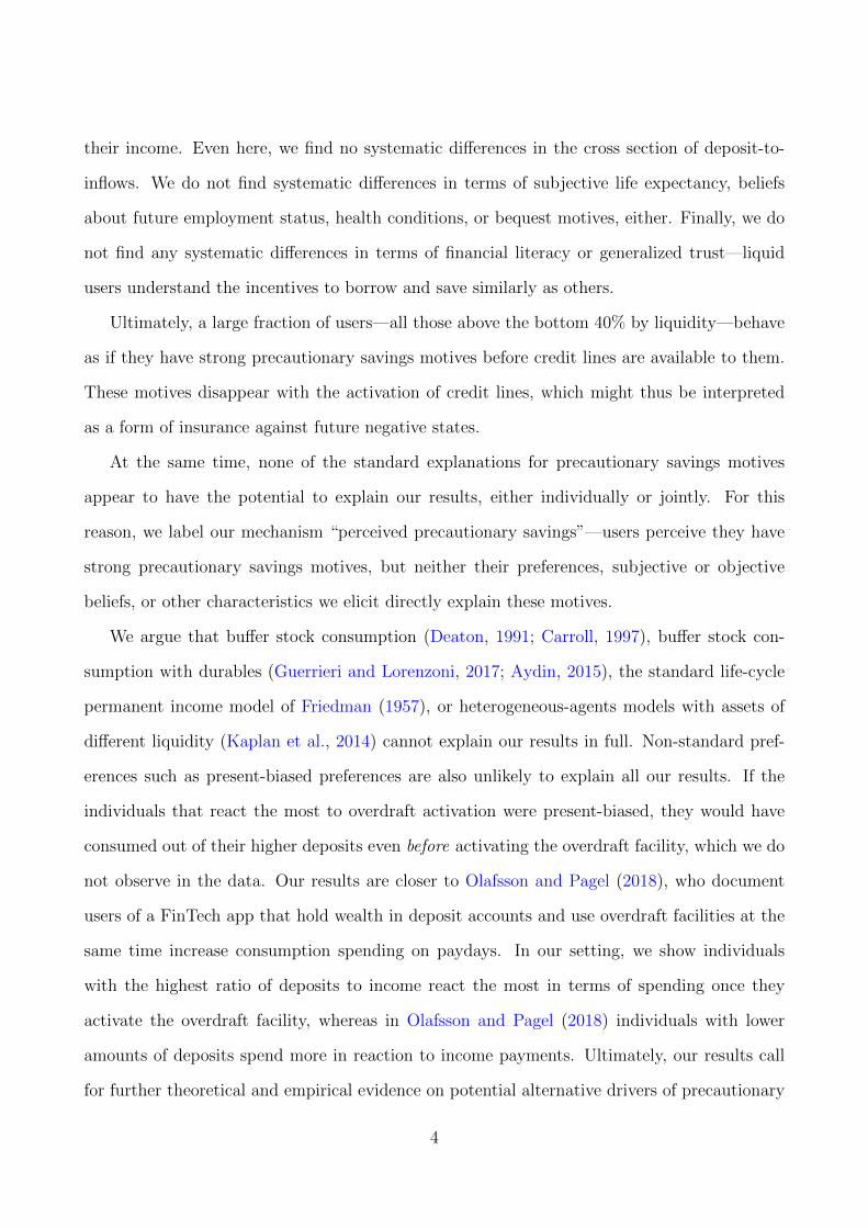
Ultimately, a large fraction of users—all those above the bottom 40% by liquidity—behave
as if they have strong precautionary savings motives before credit lines are available to them.
These motives disappear with the activation of credit lines, which might thus be interpreted
as a form of insurance against future negative states.
At the same time, none of the standard explanations for precautionary savings motives
appear to have the potential to explain our results, either individually or jointly. For this
reason, we label our mechanism “perceived precautionary savings”—users perceive they have
strong precautionary savings motives, but neither their preferences, subjective or objective
beliefs, or other characteristics we elicit directly explain these motives.
We argue that buffer stock consumption (Deaton, 1991; Carroll, 1997), buffer stock con-
sumption with durables (Guerrieri and Lorenzoni, 2017; Aydin, 2015), the standard life-cycle
permanent income model of Friedman (1957), or heterogeneous-agents models with assets of
different liquidity (Kaplan et al., 2014) cannot explain our results in full. Non-standard pref-
erences such as present-biased preferences are also unlikely to explain all our results. If the
individuals that react the most to overdraft activation were present-biased, they would have
consumed out of their higher deposits even before activating the overdraft facility, which we do
not observe in the data. Our results are closer to Olafsson and Pagel (2018), who document
users of a FinTech app that hold wealth in deposit accounts and use overdraft facilities at the
same time increase consumption spending on paydays. In our setting, we show individuals
with the highest ratio of deposits to income react the most in terms of spending once they
activate the overdraft facility, whereas in Olafsson and Pagel (2018) individuals with lower
amounts of deposits spend more in reaction to income payments. Ultimately, our results call
for further theoretical and empirical evidence on potential alternative drivers of precautionary
4
savings motives, either based on standard or non-standard beliefs.
One might wonder why we detect perceived precautionary savings motives in our setting,
but earlier research studying the effect of credit provision to households did not find this result.
The crucial difference is that we study the provision of credit lines to households that did not
have access to credit beforehand (extensive margin of credit). Most of the earlier research,
instead, is based on changing credit limits provided to households that were already borrowing
(intensive margin of credit). The insurance feature of obtaining a credit facility already exists
for borrowers that previously had access to credit, and hence the effect we document could
not arise in those earlier settings. Moreover, we find that liquid users do not tap into negative
deposits but only consume their existing savings, which suggests that changes in the credit
limits or intensive margin of credit would have no effect on them. That is to say, these users
do not make use of the credit limits at all.
A remaining concern with our baseline double-differences analysis is that users might ac-
tivate the overdraft facility endogenously when they know they are about to make a large
expense. The facts that the spending effect for liquid households is permanent, that elicited
expectations about upcoming large expenses do not differ across liquid and illiquid users, and
that we detect similar effects when limiting the analysis to users that had an account open at
least one year before the overdraft was available, reduce this concern.
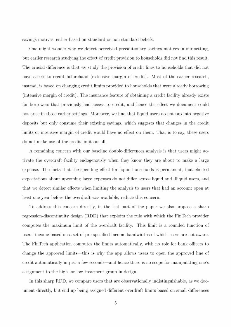
To address this concern directly, in the last part of the paper we also propose a sharp
regression-discontinuity design (RDD) that exploits the rule with which the FinTech provider
computes the maximum limit of the overdraft facility. This limit is a rounded function of
users’ income based on a set of pre-specified income bandwidths of which users are not aware.
The FinTech application computes the limits automatically, with no role for bank officers to
change the approved limits—this is why the app allows users to open the approved line of
credit automatically in just a few seconds—and hence there is no scope for manipulating one’s
assignment to the high- or low-treatment group in design.
In this sharp RDD, we compare users that are observationally indistinguishable, as we doc-
ument directly, but end up being assigned different overdraft limits based on small differences
5

in their income inflows. This assignment combines the extensive margin of credit, so that the
insurance effect of the facility exists for everybody, with a higher or lower intensive margin in
terms of credit limit. The sharp RDD confirms our results. Note that we do not use this RDD
for the baseline analysis and the heterogeneity tests, because by construction the RDD only
uses a small subset of users who are close to the sharp threshold. The RDD results thus do
not refer to the average user in our sample, and the statistical power for heterogeneity tests
in this setting is minimal by construction given that the treated and control users are almost
identical in most characteristics.
Ultimately, our results might provide novel insights about the effects of providing credit
to households along the business cycle. Providing insurance against potential negative future
spending shocks appears to increase the spending of households with high deposit-to-income
ratios, but this policy intervention would not increase their debt positions or interest payments,
because these households would not draw down from the overdraft facilities. If anything,
providing insurance to these households at times of economic slumps might increase aggregate
demand swiftly, because households that hoard cash due to perceived precautionary savings
motives might end up spending parts of their savings. Importantly, providing insurance to
perceived precautionary savers might be virtually costless based on our results, because these
individuals would not end up paying any interest, would not accumulate debt over time, and
would not worsen their credit position.
The main challenge to policies based on our findings might be political in nature. At
times of economic crisis, policy-makers would provide virtually costless insurance to wealthier
households (in terms of liquid wealth) to nudge them to spend more instead of providing
costly subsidies to poorer households, who might become risky borrowers over time. Whether
institutions might find enough political support in parliaments and among voters for this type
of policy is a matter for future research.
Methodologically, the paper suggest a compelling reason for macroeconomists to use Fin-
Tech settings for research on household borrowing, saving, and spending. Such providers allow
the researcher to access users directly in a logisitically simple way that barely involves any
6

costs, because users can be contacted interactively through the FinTech lenders’ apps. Easy
direct access to users allows the elicitation of typically unobserved characteristics, as in this
paper, as well as the potential to run field experiments to gauge the causal effects of theoretical
channels that act through preferences, beliefs, and perceptions on actual high-stake choices.
2 Institutional Setting
We cooperate with a leading European FinTech bank to test for the effects of introducing a
mobile overdraft facility on consumption spending behavior. The digital-only bank does not
operate a branch network and provides all its services through an Android or iOS mobile app.
The bank currently operates under a European banking license in several countries and has
more than 1 million customers. Users can open a bank account within 10 minutes by entering
their personal information into the app. They are required to verify their identity by providing
a copy of their passport or personal ID through video conferencing before the bank confirms
the account and users obtain their debit card by mail. The free mobile checking account is
the bank’s baseline product. The bank does not offer credit cards. Customers manage their
account entirely via the bank’s mobile app, which provides monthly consumption statistics and
allows users to set their daily payment and withdrawal limits, lock their card, or change their
pin in real time.
The bank also offers a mobile credit line in several European countries. Residents of these
countries with a sufficiently high credit score are eligible for the mobile overdraft facility.
Customers can activate the credit line directly in their mobile app within one minute and
receive a maximum overdraft amount that ranges between 500 and 5,000 Euros depending
on their credit score and other financial and personal characteristics. The bank uses a fully
automated algorithm to allocate maximum credit amounts to users. In Section 6, we describe
the bank’s loan granting and credit allocation process in detail. Users that are granted a mobile
credit line specify their desired credit amount, which they can change in real time via the mobile
app depending on their consumption needs. However, customers cannot select an amount that
7

exceeds the maximum overdraft limit granted to them by the bank. Users pay an annual
interest rate of approximately 10 percentage points on their used overdraft amount, which the
bank charges once every calendar quarter. The mobile app provides daily updated information
on users’ accrued interest costs. Customers can turn on push notifications that remind them
whenever their account balance turns negative and they start using the overdraft. The bank
cancels the mobile credit line if users default on their interest payments, receive unemployment
benefits, or experience direct debit reversals.
3 Data and Descriptive Statistics
3.1 Data Sources and Sample Selection
We obtain detailed consumption data, credit line information, and personal user characteristics
from a major European FinTech bank. Our sample consists of users that received an overdraft
between February 2015 and September 2017. We focus on individuals that the bank classifies as
“main account users” based on their consumption and inflow history to alleviate the concern
that customers might have additional accounts with other banks, which we cannot observe.
Main account users are individuals that receive a regular monthly salary or incoming standing
order into their mobile checking account for at least two consecutive months. Prior research
shows that European bank clients satisfy approximately 70% of their daily consumption needs
through their primary salary account and that the majority of individuals only have one main
account (Bain, 2017; ING, 2018). As a result, our consumption and overdraft data cover most
if not all financial activities that main account users carry out via their mobile bank account.
We obtain information about the type, amount, and timestamp of all financial transactions
that pass through users’ checking account between February 2015 and March 2019. To pro-
tect the identity of its customers, the bank rounded all transaction amounts to the nearest
Euro and only provided us with the day but not the exact time of each transaction. The
financial transactions covered by our dataset can be classified into six broad categories: (i)
8

cash deposits and withdrawals, (ii) incoming or outgoing wire transfers within the Single
Euro Payments Area (SEPA), (iii) foreign wire transfers from or to non-SEPA countries, (iv)
direct debit withdrawals (including reversals), (v) bank-imposed fees, and (vi) card-based elec-
tronic payments. The bank categorizes each electronic payment that a user makes with her
debit card into one of seventeen merchant category code (MCC) groups. MCC groups specify
the merchant’s industry and allow us to identify which type of good or service the account
holder purchased. The seventeen MCC groups cover the full range of users’ consumption
behavior and include both discretionary (e.g., entertainment, shopping, or gastronomy) and
non-discretionary consumption types (e.g., groceries, family, or utilities/furniture). Our raw
dataset contains 58,310,004 individual financial transactions, which we aggregate into user-
month observations. Each within-user time series starts with the month in which the user
signed up on the mobile app, verified her identify, and the bank then opened the account, and
ends with the closing of the account or the last month of our sample period (March 2019).
We code observations of our flow variables as zero if the user did not have any corresponding
financial transaction in the given month.
The credit line dataset contains granular information about the application date, granted
overdraft amount, and financial characteristics of users that activated the mobile overdraft
facility. We observe all user-specific input parameters that enter the bank’s credit allocation
algorithm, including each individual’s credit score, employment status, regular salary, and
other credit-relevant inflows. Since the bank shared the precise inner workings of its overdraft
granting process with us, we are able to perfectly replicate the credit allocation decision for
all mobile credit line users in our sample. Moreover, the credit dataset contains the complete
history of all overdraft setting changes that users made once they activated the credit facility.
We observe any changes in the actual overdraft usage amount and whether an individual
activated push notifications that pop-up whenever the account balance turns negative and
users start drawing on the credit line.
The bank also provides us with demographic and personal information about each main
account user. We obtain data on users’ gender, year of birth, and residential zip code. To
9

ensure data anonymity, the bank does not share the name, address, or precise date of birth of
its account holders with us. In Appendix Table A1, we define all variables that we use in our
empirical analysis.
3.2 Descriptive Statistics
Table 1 provides descriptive statistics for our main overdraft sample. We trim all ratios that
involve consumption-related variables at the 5th and 95th percentile to mitigate the impact
of outliers due to data errors or extreme values.2 Our dataset contains 603,157 user-month
observations of 36,005 individuals who obtained a mobile credit line between February 2015
and October 2017. The user base of the FinTech bank consists primarily of male Millennials who
live in urban areas. The average user in our sample is 34 years old, has monthly inflows of 2,220
Euros, and opened the mobile bank account 1.6 years ago. 79% of our sample users are male
and 53% live in large cities with more than 500,000 inhabitants. All overdraft users combined
spent a total of 441 million Euros via their mobile checking account over our sample period. On
average, these individuals consume 48% of their monthly inflows, of which approximately two
thirds are attributable to electronic card transactions and the remainder is cash consumption.
For each Euro that users spend electronically on non-discretionary goods, they purchase 61
cents of discretionary items. Main account users have access to the bank’s mobile overdraft
facility in 91% of all user-months. The average maximum overdraft amount equals about 1,561
Euros.
4 The Effect of Mobile Overdrafts on Users’
Consumption Behavior
In this section, we first assess how the average user changes her spending behavior once she
activates an overdraft facility on her mobile phone. We then move on to document a set of
2We obtain similar results when we instead winsorize our regression variables at the 5th and 95th percentileor when we use alternative trimming approaches (e.g., trimming at the 1% level in each tail).
10

heterogeneity patterns in the reaction to the availability. We find that users with higher ratios
of deposits to income flows are the ones reacting the most in terms of increasing their spending
after they obtain access to the overdraft facility.
4.1 Overall Consumption Response
Our baseline analysis considers users’ monthly consumption expenditures and uses a double-
differences (DD) design. The DD estimator compares changes in the level of spending around
the activation of mobile overdrafts between individuals that already have and the ones that have
not yet used the credit line. We restrict the analysis to mobile overdraft users only to address
the endogeneity of being eligible for the overdraft facility, which by construction depends on a
set of demographic characteristics that might also relate to changes in spending patterns over
time. Moreover, the DD design allows us to exclude the possibility that individuals who never
activate the overdraft despite being eligible might differ systematically from active users based
on unobserved characteristics that also predict their spending patterns over time, such as users’
inattention to their financial situation or the possibility that some users use the bank account
we observe only for the purpose of depositing their money and do not use such deposits for
regular consumption activities.
At the same time, the baseline DD design does not account for the possibility that unob-
served shocks at the individual level determine the timing of the overdraft facility activation
as well as consumption patterns over time. We tackle this concern directly below using a sharp
RDD that only compared users at the time they activate their facilities, relative to before.
Despite the endogeneity of the timing of activation, we use the DD design for the baseline
analysis, because this design allows us to make assessments based on the full population of
users in our sample. Instead, by construction, the RDD is based on estimating local treatment
effects among a restricted subsample of the users in the overall population, based on their
closeness to the regression discontinuity we exploit.
11

For the DD analysis, we estimate the following OLS regression model:
Consumptioni,t = β ×Overdraft Availablei,t + Fixed Effectsi,t + εi,t. (1)
The dependent variable is the sum of all cash withdrawals and debit-card transactions by
individual i in month t, divided by the amount of the user’s account inflows in month t − 1.
Our main variable of interest, Overdraft Available, is an indicator variable that equals 1 at the
beginning of the month in which the account holder got access to the credit facility on her mobile
phone. We include user fixed effects to control for time-invariant variation in consumption
patterns across overdraft users, such as differences in occupation, gender, cultural background,
or education. We also include NUTS3×year-month fixed effects to account for concurrent but
unrelated time-varying economic or institutional changes within local, sub-national districts,
called NUTS3 in the European Union, which correspond to US counties. We double cluster
standard errors at the NUTS2 (region) and year-month levels because consumption patterns
are likely to be correlated cross-sectionally and over time within closeby locations.3
In Table 2, we present the estimated effects of mobile overdraft availability on consumption
behavior. Column (1) documents an average positive consumption effect of mobile overdraft. In
terms of magnitude, overall cash and card-based consumption normalized by the user’s lagged
account inflows increases by 4.572 percentage points (t-statistic: 11.11), which corresponds to
an increase of approximately 9.5% relative to the sample mean (4.572/48.11). Columns (2)
and (3) propose a split between different means of spending. We differentiate between cash
withdrawals, i.e. cash spending, and debit-card spending. We find account holders increase
their spending significantly through both payment types. In relative terms, the increase in
card-based spending (coefficient: 3.152; t-statistic: 9.71) is larger than the increase in cash
withdrawals (coefficient: 1.345; t-statistic: 7.73), and accounts for approximately 70% of users’
3We use a broader geographic definition for the spatial clustering of standard errors, because the NUTS2level fully includes the NUTS3 level in the European Union administrative classification. This level of clusteringis more conservative than NUTS3, because it allows for correlation of unknown form across the residuals notonly across users in the same county, but also across users in neighboring counties that belong to the sameregion.
12

overall consumption response. Finally, in column (4), we study the change in the ratio be-
tween discretionary and non-discretionary spending and find users increase their discretionary
spending by 3% relative to their non-discretionary spending.
Besides the timing of access to the online facility, our DD estimates can only be interpreted
causally subject to a parallel-trends assumption—the spending behavior of treated and control
users would have followed parallel trends after the overdraft facility was available had this shock
not happened. This assumption is untestable, but we can directly test for whether the spending
behavior of treated and control users followed parallel trends before the shock. In Figure 2,
we provide graphical evidence that treated and control users have parallel and almost identical
consumption patterns during the time period leading up to the mobile overdraft activation.
To this aim, we repeat the estimation of equation (1) by adding a set of interactions of month
dummies with the baseline covariate of interest, the availability of the overdraft facility. Treated
users sharply increase their spending during the first two months in which they can access the
credit line. Subsequently, the treatment effect stabilizes at around 2% higher consumption
relative to inflows and does not fully revert in the long run. We can reject the null of no
differences between the spending of treated and control users throughout the sample period
and at any horizons we observe in the data after activation. As we will discuss below, this
timing of the effect masks substantial heterogeneity—some groups of users face a permanent
spending effect of the availability of the overdraft facility, whereas for other users the effect
dissipates over time.
5 Heterogeneity and Perceived Precautionary Savings
Our results so far have focused on average effects across users. To better understand the
economic channels that might drive our results and to assess the extent to which existing
consumption models might explain them, we turn on to study the heterogeneity of the results
in the cross section of users (Jappelli and Pistaferri, 2017).
Our baseline observational data do not include direct information about a set of economic
13

mechanisms that are crucial to assess the relevance of different models, such as risk aversion,
bequests motives, and beliefs. This lack of information typically makes it hard for empirical
studies to pin down exact channels. To solve this problem, we exploit the unique feature that
our FinTech bank can communicate with users through the online app to elicit a set of crucial
features of their preferences and beliefs directly through a survey instrument. This elicitation
is a methodological contribution of our paper and represents the main reason for why the
FinTech nature of the lender with which we cooperate is central to our analysis. Indeed,
accessing traditional bank users to elicit characteristics directly would require either inviting
these individuals to a human-subjects laboratory or sending surveys via mail or phone call,
which would limit substantially the scope and possibility of the intervention. We see our paper
as one of the very first that emphasizes the potential use of app-based online banks to elicit
characteristics of borrowers that would otherwise be barely observable in most real-time studies
of borrowing and spending.
5.1 Consumption Smoothing? Income Growth, Volatility, and Age
We start by assessing the heterogeneity of the baseline effect across two characteristics we can
observe in the field data, that is, (i) the growth of income inflows 6 months after overdraft
activation relative to 6 months before activation; and (ii) users’ age.
The permanent income hypothesis (PIH) suggests agents want to smooth their consumption
over time. Empirically, income paths are increasing early in life before flattening out. Hence,
the PIH predicts younger users and users with a steeply increasing income path should be more
likely to use the overdraft facility to smooth their consumption and borrow against their higher
future income to increase their spending on impact relative to other users.4
To assess this prediction, we split the sample in quintiles based on each of the three ob-
servable characteristics listed above. We then repeat the baseline DD analysis of equation (1)
adding a set of interactions between a dummy for whether the user belongs to each quintile of
4Not only the level, but also the uncertainty of the future income path might be relevant to predict spending(Guiso et al., 1992). We will tackle this point directly below using past income volatility as well as with asurvey instrument to elicit uncertainty about future income flows.
14

each characteristic with the treatment variable for observations before and after activation. To
make the results easier to visualize, we report the estimated coefficients and 95% confidence
intervals for each interaction in graphical form in Figure 3.
The top panel reports the effects across quintiles of income inflows growth around activation.
The estimated effect is larger for users in the first quintile relative to users in the top 3 quintiles,
although we do not reject the null hypothesis that the effects are equal across any of the
quintiles, including when we compare the size of the effect in the first and fifth quintiles. This
heterogeneity result if anything is the opposite of what the PIH would predict.
In the bottom panel of Figure 3, we split the sample into quintiles by age. Despite the fact
that our users are on average younger than the broader population, we still detect substantial
differences in age between the bottom quintile and the top quintile, whose averages are about
20 years old and 45 years old. We can plausibly argue that users across these quintiles are on
different consumption life-cycle paths. The bottom panel of Figure 3, though, shows vividly
the lack of nonlinear heterogeneities of the effect in the age distribution, but instead the effect
is stable across the whole distribution. In terms of magnitudes, we estimate coefficients that
range between 3% and 4% in each quintile. Moreover, we do not reject the null that the effects
are the same across all quintiles at any plausible level of significance and if anything, the point
estimates are slightly larger for older users with plausibly more stable income processes.
5.2 Liquidity Constraints? Deposits over Income Flows
We then move on to consider the potential role of liquidity constraints in explaining our results
(Deaton, 1991). For this analysis, we split the sample by quintiles based on the deposits-
to-income ratio in the month before activation. We use deposits-to-income as a proxy for
liquidity constraints. If liquidity constraints explained our results, we would expect that users
with lower deposits-to-income ratios would increase their spending after accessing the overdraft
facility more relative to otherwise similar users with higher deposits-to-income ratios. Indeed,
if liquidity constraints explained our baseline results, we would expect that those users with low
15

levels of liquid wealth would increase their spending once they can tap into negative deposits,
whereas users with large levels of liquid wealth would barely react to the availability of the
overdraft facility.
Figure 4 reports the results for estimating the interaction coefficients across quintiles by
deposits-to-income. We detect substantial heterogeneity in this case, but the heterogeneity of
the effects goes in the opposite direction relative to the predictions of liquidity constraints. In
fact, the effect of overdraft on spending is (insignificantly) negative for users in the bottom
quintile—the most liquidity-constrained users—and is zero for those in the second quintile.
The effect increases nonlinearly and is disproportionally higher the higher the quintile. The
estimated effect is about 2% for users in the third quintile, 5% in the fourth quintile, and
12% in the top quintile. In fact, it is the least liquidity-constrained users who increase their
spending over income flows more after having access to the overdraft facility. Although the
positive association is largest for the top quintile by deposits over income inflows, the effect
is economically and statistically significant for the median user, which suggests that specific
peculiarities of the top quintile group cannot explain the effect.
In Figure 5, we report the estimated coefficients across the deposit-to-inflows quintiles over
time. The red dashed line reports the estimated coefficients for users in the top quintile by
deposits-to-inflow, the blue solid line refers to users in the first quintile, and grey lines to users
in other quintiles. We see that not only the users in the top quintile increase their spending
more than others on impact, but their spending increases permanently and does not revert
over time. The same permanent effect is detected for users in the fourth quintile, whereas the
increase in spending reverts to zero for other users. Importantly, we detect no different trends
in the spending ratio of any users before the overdraft facility is available to them.
At first sight, the results in Figure 4 and Figure 5 might appear puzzling, because the
association between users’ pre-overdraft liquidity and their spending after overdraft activation
seems to go in the opposite direction of what we would have expected under a liquidity-
constraints explanation. Before digging deeper into the drivers of this empirical regularity, we
therefore perform a large set of robustness tests to verify that this pattern is a robust feature
16

of the data.
First, in Figure 6, we assess the robustness of the baseline pattern by liquidity quintiles
across a set of relevant subsamples and specifications. In the top left panel, we compare
the estimated coefficients and confidence intervals for the baseline specification and for the
specification in which we include the full set of controls and fixed effects in equation (1) but also
add interaction terms with user age, inflow growth in the six months before and after overdraft
availability and inflow volatility in the twelve months before the overdraft availability. We
cannot reject the null that the coefficients are equal across specifications either economically
or statistically.
In the top right panel of Figure 6, we compare the baseline effect in the full sample of users
to the results when we restrict the working sample only to users with an active account for
at least 12 months before the overdraft availability. This test is relevant, because one might
be concerned users who drive our effect were merely opening an account to take advantage of
the overdraft facility to make larger purchases and moved money from other accounts into the
online account resulting in large savings-to-deposits and large spending responses. As expected,
the estimates are substantially more noisy in the restricted sample of long-term users, but we
fail to reject the equality of the estimated coefficients either economically or statistically.
In the bottom left panel, we restrict the sample to users who spend at least 60% of their
income on average. In this test, we aim to rule out the possibility that the regularity of spending
by deposits-to-inflows is driven by users who do not use the account for spending to begin with
before the overdraft facility is available because of the availability of other accounts. We rule
out this concern directly.
Lastly, in the bottom right panel of Figure 6, we consider the robustness of our finding in
terms of the definition of our sorting variable—deposits-over-inflows. Specifically, we consider
the average effects based on whether we sort users based on the ratio measured in the month
before the overdraft facility was available or in a one-month period starting 3 months before
activation. Even in this case, we find no detectable difference in the baseline patterns.
To further assess the robustness of the baseline consumption responses based on deposits-
17
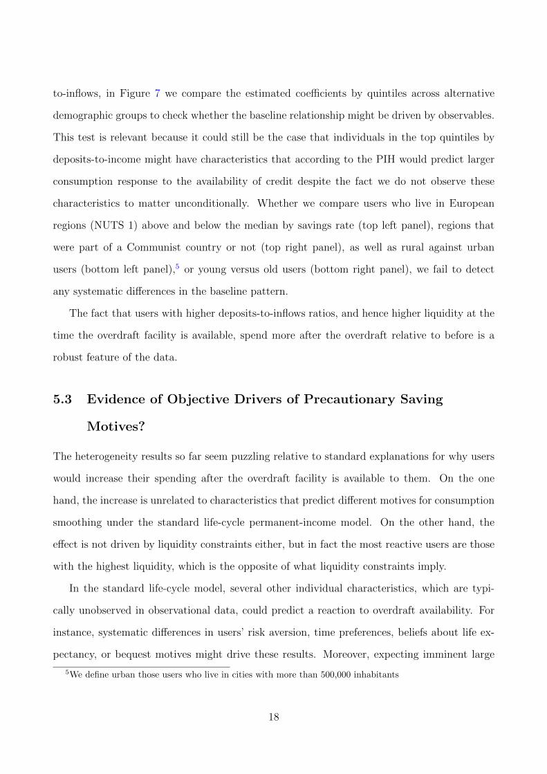
to-inflows, in Figure 7 we compare the estimated coefficients by quintiles across alternative
demographic groups to check whether the baseline relationship might be driven by observables.
This test is relevant because it could still be the case that individuals in the top quintiles by
deposits-to-income might have characteristics that according to the PIH would predict larger
consumption response to the availability of credit despite the fact we do not observe these
characteristics to matter unconditionally. Whether we compare users who live in European
regions (NUTS 1) above and below the median by savings rate (top left panel), regions that
were part of a Communist country or not (top right panel), as well as rural against urban
users (bottom left panel),5 or young versus old users (bottom right panel), we fail to detect
any systematic differences in the baseline pattern.
The fact that users with higher deposits-to-inflows ratios, and hence higher liquidity at the
time the overdraft facility is available, spend more after the overdraft relative to before is a
robust feature of the data.
5.3 Evidence of Objective Drivers of Precautionary Saving
Motives?
The heterogeneity results so far seem puzzling relative to standard explanations for why users
would increase their spending after the overdraft facility is available to them. On the one
hand, the increase is unrelated to characteristics that predict different motives for consumption
smoothing under the standard life-cycle permanent-income model. On the other hand, the
effect is not driven by liquidity constraints either, but in fact the most reactive users are those
with the highest liquidity, which is the opposite of what liquidity constraints imply.
In the standard life-cycle model, several other individual characteristics, which are typi-
cally unobserved in observational data, could predict a reaction to overdraft availability. For
instance, systematic differences in users’ risk aversion, time preferences, beliefs about life ex-
pectancy, or bequest motives might drive these results. Moreover, expecting imminent large
5We define urban those users who live in cities with more than 500,000 inhabitants
18

expenses due to unobserved health reasons, other unobserved reasons, as well as private infor-
mation about the probability of becoming unemployed and hence having more volatile income
streams in the future might all drive these results (Gomes and Michaelides, 2005; Chetty and
Szeidl, 2007; Carroll, 1997).
These dimensions might either predict larger precautionary savings motives due to prefer-
ence heterogeneity for a given level of objective uncertainty or might translate into differences
in precautionary savings due to subjective needs. Once the overdraft facility becomes available
to these users, it might act as a form of insurance and trigger higher spending, because these
users know they can now tap into negative deposits using the overdraft facility once a shock
occurs.
In addition to these precautionary savings motives, one could think about other channels
that could explain the willingness to spend liquid assets only after they obtain an overdraft
facility, which are not necessarily embedded in the standard life-cycle model. For instance, such
agents might have low financial literacy and hence are unable to optimize their allocation of
resources over time. Or, they might be distrustful of others and hence display a precautionary
saving motive that is not based on their financial conditions.
In Figure 8, we consider three dimensions that might predict differential precautionary
savings motives across quintiles by liquidity and which we can measure directly in our data.
First, we consider age. Age increases monotonically with the bins by deposits-to-income inflows,
ranging from 31.4 to 35.1. Although the difference between the fifth and first bin is statistically
different from zero, the magnitude of this difference is less that 10% of the average age in the top
bin. Most importantly, though, the typical precautionary savings explanation would suggest
that younger users have higher precautionary savings motives, because these users are likely
to have more uncertain income paths, might expect higher future income growth, might face
less employment stability, and might still not be in the workforce at all.
To further test if the standard deviation of income inflows as a proxy for income uncertainty
drives our results, we look at this variable directly in Figure 8. Specifically, we average the
standard deviation in income inflows over the 12 months before overdraft facility activation
19

across bins. We do not detect any systematic patterns or differences between the bottom
and top bin by deposits-to-income. This fact is prima facie evidence that differences in income
uncertainty do not justify why users in the top bin behave as if they have stronger precautionary
savings motives.
Another potential driver of precautionary savings motives is an increasing path of income
over time. We calculate income growth six months after the activation relative to six months be-
fore but even in this case, we do not detect any systematic patterns or economically/statistically
significant differences across bin by deposits-to-income ratios.
5.4 Eliciting Preferences, Beliefs, and Motivations
Most of the other dimensions we discuss above are typically unobservable in individual-level
data sets on borrowing and spending. Standard data sets usually only gather information about
choices, but do not include any information on agents’ preferences, beliefs, and motivations.
To make progress on this front, we exploited the unique setting of our study, which uses
data from a FinTech online-only app-based bank. We were thus able lever the feature that our
app allows accessing users directly with surveys and other instruments to elicit in real time a
large set of typically unobserved individual preferences, beliefs, and motivations.
In June and July 2019, we fielded a survey intervention we designed ad hoc to elicit users’
risk and time preferences, a large set of beliefs, motivations, perceptions, as well as financial
literacy and generalized trust. Users could answer the elicitation survey either when using
their app on the desktop version or on their mobile phones. We sent 73,000 invitations to the
survey, targeting a response rate between 10% to 15%, based on other surveys the FinTech
bank with which we cooperate ran on the platform in the past. Overall, we obtained 7,901
responses to the survey, which represents a response rate of 11%, in line with our expectations.
Of the 7,901 respondents, we kept the survey outcomes of the users for which we observe the
overdraft facility availability and activation in the time period covered by our study. Overall,
we obtain 597 unique observations of users that belong to the overdraft facility working sample
20

we used in the analysis so far and for whom we do observe all the elicited preferences and
beliefs through the survey responses.6
Importantly, when we approached users, we did not disclose that the aim of the intervention
was to link their answers to the spending behavior around the introduction of the overdraft
facility. Being silent about the overdraft facility was crucial to reduce the concern of experi-
menter demand effects, i.e., the possibility that subjects guess the aim of the experiment and
align their answers and choices to such aim. The issue of experimenter demand effects is one
of the strongest concerns faced by experimental economics and survey-based elicitation tools,
as discussed recently, for instance, by De Quidt et al. (2018). Because we did not refer to the
overdraft facility in any way within our survey, it is implausible that users would understand
that the scope of the experiment was to assess the drivers of their spending and borrowing
behaviors and hence could manipulate their answers to our questions to not disclose if and
how they consume, spend, and borrow. A drawback of the lack of direct reference to the over-
draft facility experience is that we could not ask users directly for the motivations they had
to activate and use the facility. Because of the issue of demand effects, the answers to such a
direct question would have anyway been barely interpretable due to strategic motives in users’
answers (see, e.g., D’Acunto, 2018, 2019).
To design the survey, we followed earlier research for the design of questions. We elicited
risk aversion by asking users to rank their willingness to take on risks in financial matters on a
scale from 1 (very low) to 10 (very high) (see, e.g, Guiso et al., 2008; D’Acunto et al., 2019b,c).
For time preferences, we proposed users a hypothetical choice between a certain amount at
the time of the survey or increasing amounts one month later (see, e.g., Benjamin et al., 2010;
Coibion et al., 2019). For eliciting expectations about upcoming large expenses, we asked users
to rank the probability they foresaw any large spending expenses or large medical expenses
over the following 12 months (D’Acunto et al., 2019a). We elicited similar rankings for users’
expectations about the possibility of losing their job over the following 12 months—which aims
to capture the uncertainty in their future income flows (Guiso et al., 1992)—users’ satisfaction
6We report a translation of the original survey in Appendix Table A3.
21

with their health conditions, and users’ generalized trust towards others (see, e.g., Dominitz
and Manski, 2007; Guiso et al., 2004; D’Acunto et al., 2018). To elicit users’ financial literacy,
we asked them to assess whether the amount that would compound in their checking account
at a certain interest rate would be above or below a given value (see, e.g., Lusardi and Mitchell,
2011)). Among potential questions the literature proposed for financial literacy (Lusardi and
Mitchell, 2014), we believe that the ability to understand compounding is the most relevant
in our setting, in which we study the borrowing and spending behavior of bank users when
considering the use of the overdraft facility.
Panel B of Table 3 reports the results for the basic preferences, beliefs, and motivations we
elicited. We sort users into five quintiles based on their deposit-to-income ratio before accessing
the overdraft facility. We then compute the average quantitative response of these users to the
elicitation questions within each bin, which we plot together with the 95% confidence interval
for the mean value in each quintile in Figure 9.
Across the dimensions we elicited, we fail to detect any systematic patterns in the cross-
section of liquidity—the quintiles based on value of deposits-over-income—either economically
or statistically. None of the dimensions we consider, which could have explained the pattern
in Figure 4 in a standard life-cycle consumption–savings model, seems able to capture such
pattern. Note that not only are the averages within quintiles not different from each other
statistically, but they are also similar in terms of economic magnitude, which suggests lack of
statistical power or a small sample size in the survey sample do not drive the lack of variation
across quintiles.
Overall, our evidence based on elicited preferences, beliefs, and motivations for the users
in our sample directly dismisses the most compelling traditional potential channels that would
justify a spending increase by liquid users, but not illiquid users, once the overdraft facility
was made available to them.
22

5.5 The Perceived Precautionary Savings Mechanism
The heterogeneity results suggest a pattern whereby users with higher liquidity (cash deposits)
over income react more than others to the activation of the overdraft facility in terms of
spending. This pattern is intriguing, because we might have expected the most liquid users to
be those that had the least need of an overdraft facility if they wanted to spend more before
activation. To the extent that the overdraft facility is mainly used to smooth spending and
loosen liquidity constraints, we might have expected users in the bottom quintile by deposits-
over-income would have reacted the most instead of the pattern we observe in the data.
Users that hold substantial liquidity might change their behavior after they access the over-
draft facility due to precautionary savings motives and the need to maintain enough liquidity
available in case of potential future negative income shocks.
So far, comparing bins by deposits-to-income ratios does not suggest that users in the top
bin have any objective reason to hold stronger precautionary savings motives than users in the
lower bins. We move on to assess whether, apart from increasing consumption spending after
activating the overdraft facility, users in the top bin also behave in line with precautionary
savers in terms of overdraft facility usage. In particular, precautionary savers, contrary to
liquidity-constrained individuals, would likely not tap into negative deposits and would not
increase their debt levels through the overdraft facility. Instead, they should view the facility
as a form of insurance against negative income shocks or unexpected expenses and would thus
spend some of the existing liquidity they had accumulated before the overdraft facility was
available once they know they can tap into negative deposits if needed.
The results in Figure 4 are broadly consistent with the users in the top bin by deposits-
to-income behaving as if they had strong precautionary-savings motives. First, these users are
substantially less likely than users in lower bins to tap into negative deposits after activation,
despite increasing their consumption spending relative to the pre-period substantially more
than these other users. The probability of tapping into negative deposits ranges from 67% for
users in the bottom bin to 10% for users in the top bin.
23

Because the 75th percentile of age in our sample is 38.7, it does not even seem plausible to
assume that a large fraction of the individuals in our sample might have objective precautionary
savings motives due to potentially unexpected large medical bills or other medical-related
expenses. A potential concern with our interpretation is that users decide they want to purchase
big ticket items and move cash to the deposit account at our bank before they activate the
overdraft facility. But in the data we do not observe heterogeneity in the cumulative inflows
at our bank in the three months before activation by deposits-to-income.
Overall, users with a high share of deposits to income ratios and hence high liquidity
behave as if they had precautionary savings motives and hence accumulated savings and saved
a larger share of their income before the overdraft facility became available to them. Once
they have access to the overdraft facility which acts like an insurance for additional future
spending needs, possibly due to unexpected spending needs or income shortfalls, they increase
consumption spending. These users though do not display any of the characteristics that
are typically associated with individuals that have precautionary savings motives, such as high
income volatility or higher risk aversion. Based of these considerations, we label the mechanism
we document in this paper as perceived precautionary savings motive.
5.6 Alternative Explanations and Channels
We discuss a set of possible alternative interpretations for our results. First, it is implausible
that the mobile overdraft facility loosens financial constraints on the side of users, because the
users with the highest fraction of cash deposits over income react the most to the introduction of
the overdraft facility. If anything, the consumption behavior of the most liquidity-constrained
users does not change at all.
Second, access to the overdraft facility might help users smooth consumption in case of
growing income paths. Our baseline results hold for both young and old users and life-cycle
consumption patterns are unlikely to matter for older users.7 To directly test for this mech-
7Note that our sample is younger than the average population, yet we do detect an age range of 25 yearsbetween the bottom and top quintiles of the distribution by age.
24

anism, we also study the income profiles around the overdraft activation and do not find any
evidence of different income growth across bins of deposits to income.
Third, the facility might free up liquid resources users were keeping in their bank accounts
due to precautionary motives and potential unexpected future income shocks. In this vein,
even models of buffer-stock savings that allow for both impatience and precautionary savings
motives might explain at least in part our results. Our heterogeneity results do not seem fully
consistent with this interpretation for a set of reasons. Income uncertainty decreases with age
and the heterogeneity results by age we discuss above are not consistent with this form of
precautionary-savings motive. Moreover, we find the pre-activation volatility of income flows
does not predict reaction to the availability of credit. Also, as discussed above, users close to
the liquidity constraint do not react, whereas those farther away from the constraint react the
most, and the buffer-stock interpretation predicts the opposite pattern.
A fourth potential explanation is a buffer-stock model with durable consumption similar to
the one Aydin (2015) studies. However, a set of results suggests this interpretation cannot fully
explain the results in our setting. In addition to the facts that the least liquidity-constrained
users react most and that we do not see any differential reaction based on pre-activation income
volatility, we find users that react the most on average do not tap into negative deposits and
hence de facto never use the facility.
A fifth interpretation we consider is present-biased preferences—the fact individuals dis-
count the distant future by more than they discount the immediate future (Meier and Sprenger,
2010). This interpretation by itself is unlikely to explain all our results, because if the individu-
als that react the most to overdraft activation were present-biased, they would have consumed
out of their higher deposits even before activating the overdraft facility, which we do not observe
in the data.
Contrary to the alternative explanations we have discussed in this section, the perceived
precautionary savings channel is consistent with the baseline facts we document as well as with
the fact that users at the top of the distribution by deposits over income flows react the most
to the activation of the overdraft facility.
25
At first, our results might appear inconsistent with a large literature documenting users
that are ex-ante most constrained react the most to the extension of credit (see, e.g., Agarwal
et al., 2017; Aydin, 2015; Gross and Souleles, 2002). The major difference between these
studies and our paper is the variation we exploited so far and the variation this literature uses.
Typical papers in this literature study individuals with existing access to credit with lines of
credit or credit cards and how an increase in the credit limit (i.e., an increase in the intensive
margin of credit) affects spending. A robust finding in this literature is that the ex-ante most
constrained users—users that make use of the existing credit the most—react the strongest to
the intensive margin extension of credit which is a natural finding. In our case, instead, we
study how individuals that previously did not have access to credit adjust their spending to the
availability of the overdraft facility, an extensive margin of credit. In our setting, it appears
natural that users that previously were most concerned about future unexpected expenses or
had higher precautionary savings demands for other reasons which we capture by sorting on
deposits-to-income react the most to the provision of a downside insurance.
6 Regression Discontinuity Analysis
A remaining concern with our analysis so far relates to the identification of a causal effect of
the overdraft availability on spending choices. As discussed above, the timing at which users
open their accounts might coincide with the availability of the overdraft facility, for instance
because users plan large future expenses. The test in which we only consider users who had
an account with our provider open at least one year before the overdraft facility was made
available reduces this concern.
At the same time, other omitted variables might simultaneously impact users’ consumption
behavior and overdraft activation decision, giving rise to a spurious relation between the two.
One example for such a correlated omitted variable might be time-varying, user-specific expo-
sure to television commercials that independently advertise the bank’s overdraft and various
consumer products, even for users who have been banking with our provider for quite some
26

time and hence do not open new accounts.
To directly address these endogeneity concerns, in this last part of the paper we estimate the
causal effects of mobile overdraft on spending in a sharp RDD that exploits variation in users’
overdraft limits based on thresholds embedded in the bank’s credit allocation algorithm. Our
sharp RDD conditions the analysis on users’ (possibly endogenous) selection into the mobile
overdraft and relies on exogenous variation in the size of the credit line along the intensive
margin.
We do not implement this design for the baseline analysis of the paper because we can
only exploit a limited number of users in the sample for the RDD setting. By construction, as
we discuss in more detail below, the RDD only employes users who lie close to pre-specified
thresholds based on the algorithm that assigns the overdraft amount to those activating an
overdraft facility. Because of the limited sample, unfortunately any meaningful statistical
analysis of heterogeneity and variation across subgroups of users would be impossible.
6.1 Credit Allocation Algorithm
The bank’s credit allocation process consists of two steps. First, the bank determines whether
users pass all exclusion criteria and are thus eligible for a mobile credit line. Overdraft appli-
cants receive a credit line if they (i) are employed, (ii) live in countries where the bank offers
a mobile overdraft, (iii) have a minimum credit score of F , and (iv) their checking account
did not trigger any direct debit reversals. The bank obtains credit scores from consumer credit
bureaus, which collect information on users’ credit histories to estimate default probabilities
and assign individual credit ratings from A (lowest default risk) to M (highest default risk). A
credit score of F implies that the individual has an estimated default probability of less than
10 percent.
Second, the bank determines the maximum overdraft amount for each eligible user based
27

on the applicant’s credit score and average account income according to the following formula:
Overdraft Amount =
Max Limit if 2× Income ≥ Max Limit
Min Limit if 2× Income ≤ Min Limit
250× b2×·Income250
e otherwise,
(2)
where bxe rounds the number x to the nearest integer.
For each rating notch between A and F, the bank specifies a lower (Min Limit) and upper
limit (Max Limit) for each user’s allocated credit amount. Income is a linear function of
the user’s different inflow types in the months prior to the overdraft application. Our data
sharing agreement with the bank does not allow us to report the rating-specific overdraft
limits or the precise formula that transforms users’ account inflows into income. However, we
can disclose that the bank differentiates between regular salary and non-salary related inflows
(e.g., pensions, child benefits, study support from parents etc.) and puts a higher weight on
the former. The lower and upper overdraft limits monotonically increase in the customer’s
credit rating and range between 500 and 5,000 Euros.
To determine each user’s maximum available overdraft amount, the bank’s fully automated
credit allocation algorithm multiplies the Income variable by 2. If the resulting value exceeds
(falls below) the upper (lower) credit limit, the maximum overdraft amount is bounded from
above (below) by the rating-specific limit. If the doubled income falls in between the upper
and lower limit, the amount is rounded to the closest 250 Euro multiple at the midpoint.
Panel A of Figure 10 illustrates the rounding convention embedded in the credit algorithm.
For example, if overdraft applicant A has a salary of 2,100 Euros and no additional account
inflows, her implied overdraft amount after multiplying the income by 2 equals 4,200 Euros,
which, if rounded to the closest 250 Euro threshold, translates into a maximum available
overdraft amount of 4,250 Euros (assuming that the upper and lower credit limits do not bite).
The bank’s credit allocation process gives rise to 18 unique thresholds in the interval between
500 and 5,000 Euros, at which the maximum overdraft amount jumps discontinuously by 250
28
Euros. At these thresholds, users with almost identical income that find themselves on opposite
sides of the rounding threshold receive different overdraft limits for plausibly exogenous reasons.
Crucially, users are not aware of the algorithm and the algorithm is fully automated leaving
no room for human intervention.
6.2 Empirical Implementation
We limit our analysis to users whose maximum overdraft amount equals the individual’s income
multiplied by two and rounded to the nearest multiple of 250. That is, we drop all users whose
transformed income exceeds or falls below the upper or lower credit limit (within the given
rating notch) such that the rounding thresholds embedded in the bank’s credit allocation
algorithm do not affect the maximum overdraft amount. For each user in our RDD sample,
we compute the forcing variable Xi, which quantifies the individual’s distance (in Euros) to
the nearest rounding threshold. Xi removes differences in absolute rounding thresholds across
individuals and is centered around zero. Users with Xi ≥ 0 are treated and receive a maximum
overdraft amount that is 250 Euros higher than those of control users for whom Xi < 0. The
probability that a user’s overdraft limit gets rounded up by 250 Euros changes discontinuously
from 0 to 1 at the rounding threshold. Panel B of Figure 10 illustrates the exact treatment
rule of our sharp RDD and plots users’ treatment assignment for different values of the forcing
variable Xi. In areas close to the rounding threshold (where Xi = 0), treated and control users
have almost identical income profiles.
To examine the causal effect of mobile credit lines on users’ consumption behavior, we
implement the following sharp RDD:
τ ≡ E (Ci(1)|Xi = 0)− E (Ci(0)|Xi = 0) . (3)
τ is the RD treatment effect and Ci(1/0) is the change in treated (1) or control (0) user’s
average consumption three months before and after the credit allocation decision, divided by
the individual’s average inflows in the three months prior to the overdraft application. To
29

estimate this model, we fit a weighted least squares regression of the observed consumption
change on a constant and polynomials of Xi on both sides of the rounding threshold. The
RD treatment effect is the difference in estimated intercepts from these two local weighted
regressions. Formally, each user’s consumption change equals:
Ci =
Ci(0) if Xi ≥ 0
Ci(1) if Xi < 0.
(4)
We focus on observations within the interval [−h, h] around the rounding threshold, where
h > 0 denotes our bandwidth. The kernel function K(·) specifies our regression weights. µ+/−
is the estimate of E (Ci(1/0)|Xi = 0) for observations above or below the threshold, which we
define as:
Ci = µ+/− +
p∑j=1
µ+/−,jXji , (5)
where p denotes to the order of our local polynomial. The RD treatment effect then equals:
τ = µ+ − µ−. (6)
To operationalize the RD estimator, we need to specify (i) the order of polynomial p, (ii) the
kernel function K(·), and (iii) the bandwidth h. We follow Gelman and Imbens (2018) and only
use polynomials of order 1 and 2 to avoid overfitting issues. We apply weights from a triangular
kernel because it is the mean squared error (MSE) minimizing choice for point estimation in
our context (Cheng et al., 1997). Finally, we employ the MSE-optimal bandwidth selection
procedure recommended by Calonico et al. (2014), which corrects for the non-negligible bias
resulting from subjective bandwidth choices. We residualize the outcome variables of our RD
analysis with NUTS3×year-month fixed effects to ensure that we compare treated and control
users from the same European country at a similar point in time.
30

6.3 Assessing Identification Assumptions: Treatment
Manipulation and Balancing Tests
Our sharp RDD critically relies on the assumption that the forcing variable for individuals
just below the threshold is similar to those just above the threshold. If users can manipulate
the forcing variable and thereby their assignment to treatment and control groups, this local
continuity assumption is violated, which results in biased RD estimates (Roberts and Whited,
2013).
Conceptually, it is unlikely that users can control their treatment assignment in our setting.
Most importantly, the bank’s credit allocation algorithm is proprietary information and not
known by overdraft users. Even if individuals were informed about the precise inner workings
of the overdraft allocation formula (in particular its rounding thresholds), it seems implausible
that users could precisely manipulate their income, for example, by negotiating a higher wage
with their employer (Lee and Lemieux, 2010). Moreover, it appears unlikely that overdraft
users would be willing to voluntarily forgo parts of their salary just to obtain access to a higher
credit limit.
To formally assess the validity of the local continuity assumption, we test for the presence
of a discontinuity in the density of Xi at the rounding threshold. If users systematically inflate
their income to receive a higher overdraft limit, we should observe a kink in the distribution
of our forcing variable right above the threshold. We use the local polynomial density esti-
mator of Cattaneo et al. (2017) to test whether overdraft users manipulate their assignment
into treatment and control group. In Appendix Figure A1, we plot both the frequency distri-
bution (Panel A) and density function based on quadratic local polynomials (Panel B) of our
running variable and do not find graphical evidence for bunching above the rounding thresh-
old. In Figure A2 in the Appendix, we report the estimation results of the formal treatment
manipulation test by Cattaneo et al. (2017) for different polynomial and bandwidth choices.
In all specifications, we fail to reject the null hypothesis that our running variable is locally
continuous around the rounding threshold.
31
The local continuity assumption implies that individuals below and above the cutoff should
not only be similar in terms of the forcing variable but also along other characteristics. Since
overdraft users lack the ability to precisely manipulate their distance to the rounding threshold,
no systematic differences in observable characteristics between the two groups of individuals
should exist. Consistent with this argument, we do not find significant differences in the average
age, gender, time since account opening, account inflows, and consumption between treated
and control users prior to the activation of the mobile overdraft. As an alternative balancing
test, we repeat our RD analysis but replace our main outcome variable with each observable
user characteristic. In Table A2 of the Appendix, we document the RD treatment effect for all
our covariates is economically and statistically indistinguishable from zero.
Overall, the evidence in this subsection indicates that overdraft users do not manipulate
their treatment assignment and that individuals above and below the rounding threshold have
similar observable characteristics. Both findings suggest the local continuity assumption is
satisfied and thereby corroborates the internal validity of our sharp RD design.
6.4 RD Consumption Effect
In Figure 11, we graphically illustrate the RD treatment effect of a 250 Euro higher overdraft
limit on users’ consumption behavior. We aggregate our data into disjoint bins and make sure
each bin contains either treatment or control observations. We then calculate the average value
of our outcome variable, plot this value above the midpoint of the bin, and separately fit two
linear regressions through all observations on each side of the rounding threshold.
In Panel A of Figure 11, we verify that individuals just above the threshold indeed receive
a higher maximum overdraft amount (relative to their income) compared to users just below
the threshold. The slope of both fitted regressions lines is negative since, within treatment
and control group, individuals with larger values of our forcing variable Xi have a higher
income, which we use to normalize users’ overdraft limit. In Panel B, we plot the change in
average (normalized) consumption three months before and after the user obtained access to
32

the credit line. We find a positive discontinuity in users’ consumption growth right at the
rounding threshold, indicating treated users consume more relative to control users following
the exogenous assignment of a 250 Euro higher overdraft limit. In Table 5, we present the
coefficients from estimating the sharp RD design we formalized in equations (3) to (6). We
estimate first- and second-order polynomial regressions at the rounding threshold and report
both bias-corrected and conventional t-statistics (Cattaneo et al., 2017; Gelman and Imbens,
2018). In columns (1) and (2), we document a positive and highly statistically significant RD
treatment effect on users’ consumption growth. The coefficient estimates do not attenuate
when we add user characteristics as control variables in a linear and additive-separable way. In
line with Calonico et al. (2019), we find adding covariates increases the precision of our point
estimates, which again suggests the local continuity assumption is satisfied.
We conduct two robustness tests to assess the sensitivity of our RD estimates. First, we
examine how sensitive the RD results are with respect to the choice of our bandwidth (Imbens
and Lemieux, 2008). Varying the bandwidth is only meaningful over small intervals around the
MSE-optimal choice (Cattaneo et al., 2020). Bandwidths much larger than the MSE-optimal
bandwidth bias the RD estimator, while substantially smaller bandwidths inflate its variance.
Figure A3 in the Appendix shows different bandwidth choices do neither substantially affect
the magnitude of the point estimate, nor its significance. Second, we assess how robust our
RD point estimates are to excluding data close to the threshold (see, e.g., Barreca et al., 2011,
2016). We drop users located within the radius r > 0 of the rounding cutoff, that is, we
exclude observations for which |Xi| ≤ r (Cattaneo et al., 2020). Appendix Figure A4 plots the
coefficient estimates for different choices of r and shows that observations close to the rounding
threshold do not drive our results.
7 Conclusion
We study the consumption response to the introduction of an overdraft facility on a FinTech
app. The average user increases her consumption spending over income by 4.5 percentage
33

points on impact relative to similar users that have access to the overdraft facility at a later
point in time. The increase in consumption is permanent and we observe a reallocation of
consumption from discretionary to non-discretionary expenses. For identification, we exploit
a sharp regression discontinuity design exploiting different sizes of overdraft based on income
and confirm our baseline findings.
When we study heterogeneity in the response by observables, we observe a similar response
for young and old users, for users with low and high income volatility, and for users with steep
and flat income paths. When we split the sample based on the ratio of deposits over inflows, we
find instead a large consumption response for users with high liquid savings, whereas the users
with the lowest amount of liquid savings do not react at all to the provision of the overdraft
facility. These results are not fully consistent with myopic consumers, models with financial
constraints, buffer stock models (with durables) and present bias and the canonical life-cycle
permanent income model.
Additional results, instead, suggest a perceived precautionary savings channel is at work for
users with high deposits over inflow. Before the facility is available, they perceive high income
risk or future expenses and consequently save. Once the overdraft facility is available, which
acts like an insurance against future shortfalls, they increase their consumption substantially
but barely make use the overdraft facility.
Our findings open exciting new avenues for future research. What are the microfoundations
of perceived precautionary savings motives? In particular, does this attitude results from biased
beliefs about the likelihood of future negative states of the world or is it instead consistent with
the neoclassical consumption model in a setting in which consumers have high risk aversion?
In terms of policy and real-world applications, do perceived precautionary savings change the
effectiveness of conventional fiscal policy such as tax rebates? And could policies be designed
to insure perceived precautionary savers in bad times and nudge them to spend their cash in
times in which higher aggregate demand is needed?
34

References
Agarwal, S., Chomsisengphet, S., Mahoney, N., Stroebel, J., 2017. Do Banks Pass ThroughCredit Expansions to Consumers Who Want to Borrow? Quarterly Journal of Economics133, 129–190.
Aydin, D., 2015. The Marginal Propensity to Consume Out of Liquidity: Evidence fromRandom Assignment of 54,522 Credit Lines. Working Paper. Stanford University.
Bain, 2017. Evolving the Customer Experience in Banking. https://www.bain.com/insights/evolving-the-customer-experience-in-banking, accessed on january 3, 2019. Bain &Company Inc.
Baron, M., Xiong, W., 2017. Credit Expansion and Neglected Crash Risk. Quarterly Journalof Economics 132, 713–764.
Barreca, A.I., Guldi, M., Lindo, J.M., Waddell, G.R., 2011. Saving Babies? Revisiting theEffect of Very Low Birth Weight Classification. Quarterly Journal of Economics 126, 2117–2123.
Barreca, A.I., Lindo, J.M., Waddell, G.R., 2016. Heaping-Induced Bias in Regression Discon-tinuity Designs. Economic Inquiry 54, 268–293.
Ben-David, I., Fermand, E., Kuhnen, C.M., Li, G., 2018. Expectations Uncertainty and House-hold Economic Behavior. Working Paper. National Bureau of Economic Research.
Benjamin, D.J., Choi, J.J., Strickland, A.J., 2010. Social Identity and Preferences. AmericanEconomic Review 100, 1913–28.
Calonico, S., Cattaneo, M.D., Farrell, M.H., Titiunik, R., 2019. Regression DiscontinuityDesigns Using Covariates. Review of Economics and Statistics 101, 442–451.
Calonico, S., Cattaneo, M.D., Titiunik, R., 2014. Robust Nonparametric Confidence Intervalsfor Regression-Discontinuity Designs. Econometrica 82, 2295–2326.
Carroll, C.D., 1997. Buffer-Stock Saving and the Life Cycle/Permanent Income Hypothesis.Quarterly Journal of Economics 112, 1–55.
Cattaneo, M.D., Idrobo, N., Titiunik, R., 2020. A Practical Introduction to Regression Dis-continuity Designs. Elements in Quantitative and Computational Methods for the SocialSciences, Cambridge University Press.
Cattaneo, M.D., Jansson, M., Ma, X., 2017. Simple Local Polynomial Density Estimators.Working Paper. University of Michigan.
Cheng, M.Y., Fan, J., Marron, J.S., 1997. On Automatic Boundary Corrections. The Annalsof Statistics 25, 1691–1708.
Chetty, R., Szeidl, A., 2007. Consumption Commitments and Risk Preferences. QuarterlyJournal of Economics 122, 831–877.
35

Coibion, O., Gorodnichenko, Y., Weber, M., 2019. Monetary Policy Communications and theirEffects on Household Inflation Expectations. Working Paper. National Bureau of EconomicResearch.
D’Acunto, F., 2018. Identity and Choice Under Risk. Working Paper. Boston College.
D’Acunto, F., 2019. Tear Down This Wall Street: Anti-finance Rhetoric, Subjective Beliefs,and Investment. Working Paper. Boston College.
D’Acunto, F., Hoang, D., Paloviita, M., Weber, M., 2019a. IQ, Expectations, and Choice.Working Paper. National Bureau of Economic Research.
D’Acunto, F., Malmendier, U., Ospina, J., Weber, M., 2019b. Exposure to Daily Price Changesand Inflation Expectations. Working Paper. National Bureau of Economic Research.
D’Acunto, F., Malmendier, U., Weber, M., 2019c. Traditional Gender Norms Distort Women’sEconomic Expectations. Working Paper. Booth School of Business.
D’Acunto, F., Prokopczuk, M., Weber, M., 2018. Historical Antisemitism, Ethnic Specializa-tion, and Financial Development. Review of Economic Studies 86, 1170–1206.
De Quidt, J., Haushofer, J., Roth, C., 2018. Measuring and Bounding Experimenter Demand.American Economic Review 108, 3266–3302.
Deaton, A., 1991. Saving and Liquidity Constraints. Econometrica 59, 1221–48.
Di Maggio, M., Kermani, A., 2017. Credit-Induced Boom and Bust. Review of FinancialStudies 30, 3711–3758.
Dominitz, J., Manski, C.F., 2007. Expected Equity Returns and Portfolio Choice: Evidencefrom the Health and Retirement Study. Journal of the European Economic Association 5,369–379.
Friedman, M., 1957. The Permanent Income Hypothesis, in: A Theory of the ConsumptionFunction. Princeton University Press, pp. 20–37.
Gelman, A., Imbens, G., 2018. Why High-Order Polynomials Should Not Be Used in RegressionDiscontinuity Designs. Journal of Business & Economic Statistics 0, 1–10.
Gomes, F., Michaelides, A., 2005. Optimal Life-Cycle Asset Allocation: Understanding theEmpirical Evidence. Journal of Finance 60, 869–904.
Gross, D.B., Souleles, N.S., 2002. Do Liquidity Constraints and Interest Rates Matter forConsumer Behavior? Evidence from Credit Card Data. Quarterly Journal of Economics117, 149–185.
Guerrieri, V., Lorenzoni, G., 2017. Credit Crises, Precautionary Savings, and the LiquidityTrap. Quarterly Journal of Economics 132, 1427–1467.
Guiso, L., Jappelli, T., Terlizzese, D., 1992. Earnings Uncertainty and Precautionary Saving.Journal of Monetary Economics 30, 307–337.
36

Guiso, L., Sapienza, P., Zingales, L., 2004. The Role of Social Capital in Financial Development.American Economic Review 94, 526–556.
Guiso, L., Sapienza, P., Zingales, L., 2008. Trusting the Stock Market. Journal of Finance 63,2557–2600.
Imbens, G.W., Lemieux, T., 2008. Regression Discontinuity Designs: A Guide to Practice.Journal of Econometrics 142, 615–635.
ING, 2018. International Survey Mobile Banking 2018. https://www.ezonomics.com/ing international surveys/mobile-banking-2018, accessed on january 3, 2019. ING-DiBa AG.
Jappelli, T., Pistaferri, L., 2017. The Economics of Consumption: Theory and Evidence.Oxford University Press.
Kaplan, G., Violante, G.L., Weidner, J., 2014. The Wealthy Hand-to-Mouth. Brookings Paperson Economic Activity , 77–153.
Lee, D.S., Lemieux, T., 2010. Regression Discontinuity Designs in Economics. Journal ofEconomic Literature 48, 281–355.
Lusardi, A., Mitchell, O.S., 2011. Financial Literacy and Planning: Implications for RetirementWellbeing. Working Paper. National Bureau of Economic Research.
Lusardi, A., Mitchell, O.S., 2014. The Economic Importance of Financial Literacy: Theoryand Evidence. Journal of Economic Literature 52, 5–44.
Meier, S., Sprenger, C., 2010. Present-Biased Preferences and Credit Card Borrowing. Ameri-can Economic Journal: Applied Economics 2, 193–210.
Mian, A., Sufi, A., 2015. House of Debt: How They (and You) Caused the Great Recession,and How We Can Prevent it from Happening Again. University of Chicago Press .
Mian, A., Sufi, A., Verner, E., 2017. Household Debt and Business Cycles Worldwide. QuarterlyJournal of Economics 132, 1755–1817.
Olafsson, A., Pagel, M., 2018. The Liquid Hand-to-Mouth: Evidence from Personal FinanceManagement Software. Review of Financial Studies 31, 4398–4446.
Roberts, M.R., Whited, T.M., 2013. Endogeneity in Empirical Corporate Finance, in: Hand-book of the Economics of Finance. Elsevier. volume 2, pp. 493–572.
Schularick, M., Taylor, A.M., 2012. Credit Booms Gone Bust: Monetary Policy, LeverageCycles, and Financial Crises, 1870-2008. American Economic Review 102, 1029–61.
37

Tables and Figures
Figure 2: Consumption Pattern around Overdraft Availability
Overdraft Available
-8%
-4%
0%4%
8%12
%C
onsu
mpt
ion t
/ In
flow
s t-1
t≤-6 t-5 t-4 t-3 t-2 t-1 t t+1 t+2 t+3 t+4 t+5 t≥6Months relative to Treatment
Notes: This figure shows coefficient estimates and 95% confidence intervals for OLS regressions esti-mating the effect of mobile overdrafts on users’ consumption behavior. We estimate model (1) fromTable 2 but replace the Overdraft Available indicator with separate time dummies, each marking aone-month period (except for event period t− 1).
38

Figure 3: Intertemporal Consumption Smoothing?
-2%
0%2%
4%6%
8%C
onsu
mpt
ion
/ Inf
low
s
Q1 Q2 Q3 Q4 Q5Inflows Growth Quintile
-2%
0%2%
4%6%
8%C
onsu
mpt
ion
/ Inf
low
s
Q1 Q2 Q3 Q4 Q5Age Quintile
Notes: This figure illustrates the cross-sectional heterogeneity in users’ consumption response to the mobileoverdraft. To generate these plots, we take the cross-section of users at their treatment date and assign theminto non-overlapping quintiles from lowest (1st quintile) to highest (5th quintile) based on the underlying usercharacteristic. We then interact each of the 5 quintile indicators with a dummy variable that equals 1 if theuser has access to a mobile overdraft in the given month. Vertical bands represent 95% confidence intervals forthe point estimates of each quintile. We double cluster standard errors at the NUTS2 and year-month level.
39

Figure 4: Consumption Response by Deposit-to-Income Quintile-4
%0%
4%8%
12%
16%
Con
sum
ptio
n / I
nflo
ws
Q1 Q2 Q3 Q4 Q5Deposits / Inflows Quintile
Notes: This figure illustrates the cross-sectional heterogeneity in users’ consumption response to the mobileoverdraft. To generate this plot, we take the cross-section of users at their treatment date and assign theminto non-overlapping quintiles from lowest (1st quintile) to highest (5th quintile) based on the underlying usercharacteristic. We then interact each of the 5 quintile indicators with a dummy variable that equals 1 if theuser has access to a mobile overdraft in the given month. Vertical bands represent 95% confidence intervals forthe point estimates of each quintile. We double cluster standard errors at the NUTS2 and year-month level.
40

Figure 5: Consumption Pattern by Deposit-to-Income Quintile
Overdraft Available
-10%
0%10
%20
%30
%40
%C
onsu
mpt
ion t
/ In
flow
s t-1
t≤-6 t-5 t-4 t-3 t-2 t-1 t t+1 t+2 t+3 t+4 t+5 t≥6Months relative to Treatment
Q2 Q3 Q4 Q1 Q5
Notes: This figure shows coefficient estimates and 95% confidence intervals for OLS regressions estimating theheterogeneous effect of mobile overdrafts on the consumption behavior of users with different ex-ante liquidity.To generate this plot, we take the cross-section of users at their treatment date and assign them into non-overlapping quintiles from lowest (1st quintile) to highest (5th quintile) based on the deposit to inflows ratio inthe month before treatment. We estimate model (1) from Table 2 but replace the Overdraft Available indicatorwith separate time dummies, which we further interact with our quintile indicators. Each time dummy marks aone-month period (except for event period t− 1). Coefficients are normalized by subtracting the pre-treatmentmean for each quintile. We double cluster standard errors at the NUTS2 and year-month level.
41
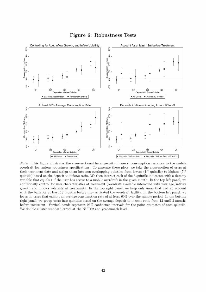
Figure 6: Robustness Tests
-5%
0%5%
10%
15%
20%
Con
sum
ptio
n / I
nflo
ws
Q1 Q2 Q3 Q4 Q5Deposits / Inflows Quintile
Baseline Specification Additional Controls
Controlling for Age, Inflow Growth, and Inflow Volatility
-5%
0%5%
10%
15%
20%
Con
sum
ptio
n / I
nflo
ws
Q1 Q2 Q3 Q4 Q5Deposits / Inflows Quintile
All Users At least 12 Months
Account for at least 12m before Treatment
-6%
0%6%
12%
18%
24%
Con
sum
ptio
n / I
nflo
ws
Q1 Q2 Q3 Q4 Q5Deposits / Inflows Quintile
All Users Subsample
At least 60% Average Consumption Rate-5
%0%
5%10
%15
%20
%C
onsu
mpt
ion
/ Inf
low
s
Q1 Q2 Q3 Q4 Q5Deposits / Inflows Quintile
Deposits / Inflows in t-1 Deposits / Inflows from t-12 to t-3
Deposits / Inflows Grouping from t-12 to t-3
Notes: This figure illustrates the cross-sectional heterogeneity in users’ consumption response to the mobileoverdraft for various robustness specifications. To generate these plots, we take the cross-section of users attheir treatment date and assign them into non-overlapping quintiles from lowest (1st quintile) to highest (5th
quintile) based on the deposit to inflows ratio. We then interact each of the 5 quintile indicators with a dummyvariable that equals 1 if the user has access to a mobile overdraft in the given month. In the top left panel, weadditionally control for user characteristics at treatment (overdraft available interacted with user age, inflowsgrowth and inflows volatility at treatment). In the top right panel, we keep only users that had an accountwith the bank for at least 12 months before they activated the overdraft facility. In the bottom left panel, wefocus on users that exhibit an average consumption rate of at least 60% over the sample period. In the bottomright panel, we group users into quintiles based on the average deposit to income ratio from 12 until 3 monthsbefore treatment. Vertical bands represent 95% confidence intervals for the point estimates of each quintile.We double cluster standard errors at the NUTS2 and year-month level.
42
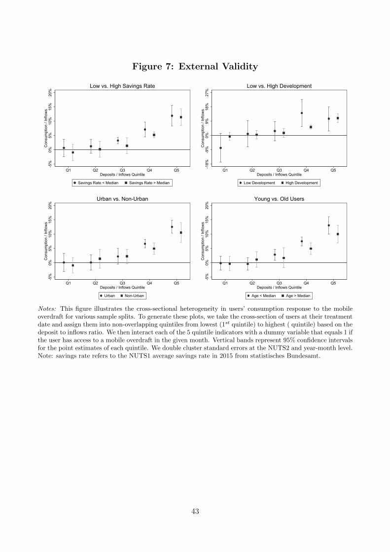
Figure 7: External Validity
-5%
0%5%
10%
15%
20%
Con
sum
ptio
n / I
nflo
ws
Q1 Q2 Q3 Q4 Q5Deposits / Inflows Quintile
Savings Rate < Median Savings Rate > Median
Low vs. High Savings Rate
-18%
-9%
0%9%
18%
27%
Con
sum
ptio
n / I
nflo
ws
Q1 Q2 Q3 Q4 Q5Deposits / Inflows Quintile
Low Development High Development
Low vs. High Development
-5%
0%5%
10%
15%
20%
Con
sum
ptio
n / I
nflo
ws
Q1 Q2 Q3 Q4 Q5Deposits / Inflows Quintile
Urban Non-Urban
Urban vs. Non-Urban-5
%0%
5%10
%15
%20
%C
onsu
mpt
ion
/ Inf
low
s
Q1 Q2 Q3 Q4 Q5Deposits / Inflows Quintile
Age < Median Age > Median
Young vs. Old Users
Notes: This figure illustrates the cross-sectional heterogeneity in users’ consumption response to the mobileoverdraft for various sample splits. To generate these plots, we take the cross-section of users at their treatmentdate and assign them into non-overlapping quintiles from lowest (1st quintile) to highest ( quintile) based on thedeposit to inflows ratio. We then interact each of the 5 quintile indicators with a dummy variable that equals 1 ifthe user has access to a mobile overdraft in the given month. Vertical bands represent 95% confidence intervalsfor the point estimates of each quintile. We double cluster standard errors at the NUTS2 and year-month level.Note: savings rate refers to the NUTS1 average savings rate in 2015 from statistisches Bundesamt.
43

Figure 8: User Characteristics by Deposit-to-Income Quintile
2830
3234
3638
Q1 Q2 Q3 Q4 Q5Deposits / Inflows Quintile
Age (at Treatment)
600
800
1000
1200
1400
1600
Q1 Q2 Q3 Q4 Q5Deposits / Inflows Quintile
Inflows Volatility (over last 12 Months)
-2%
0%2%
4%6%
8%
Q1 Q2 Q3 Q4 Q5Deposits / Inflows Quintile
Inflows Growth (over last and next 6 Months)
Notes: This figure illustrates the cross-sectional heterogeneity in users’ characteristics by deposits to inflowsquintile. To generate these plots, we take the cross-section of users at their treatment date and assign theminto non-overlapping quintiles from lowest (1st quintile) to highest (5th quintile) based on the deposit to inflowsratio in the month before treatment. Vertical bands represent 95% confidence intervals for the mean of eachquintile.
44

Figure 9: Subjective Beliefs by Deposit-to-Income Quintile
02
46
810
Q1 Q2 Q3 Q4 Q5Deposits / Inflows Quintile
Risk Aversion
100
110
120
130
140
150
Q1 Q2 Q3 Q4 Q5Deposits / Inflows Quintile
Patience0
24
68
10
Q1 Q2 Q3 Q4 Q5Deposits / Inflows Quintile
Likelihood of Large Expenses - 12m Horizon
02
46
810
Q1 Q2 Q3 Q4 Q5Deposits / Inflows Quintile
Likelihood of Large Medical Expenses - 12m Horizon
02
46
810
Q1 Q2 Q3 Q4 Q5Deposits / Inflows Quintile
Likelihood of Loosing Job
02
46
810
Q1 Q2 Q3 Q4 Q5Deposits / Inflows Quintile
Health Satisfaction
6070
8090
100
110
Q1 Q2 Q3 Q4 Q5Deposits / Inflows Quintile
Life Expectancy
020
4060
8010
0
Q1 Q2 Q3 Q4 Q5Deposits / Inflows Quintile
Can Perform Simple Financial Computation (% within Q)
Notes: This figure plots a set of preferences and beliefs dimensions we elicited from users through an ad-hocsurvey intervention. To generate these plots, we take the cross-section of users at their treatment date andassign them into non-overlapping quintiles from lowest (1st quintile) to highest (5th quintile) based on the ratioof deposited amount over income. We limit the sample to users that activate the overdraft facility in our mainsample. Vertical bands represent 95% confidence intervals for the point estimates of each quintile.
45
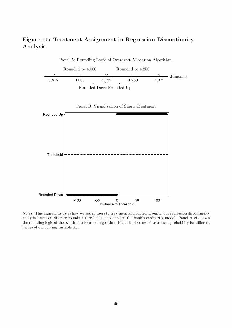
Figure 10: Treatment Assignment in Regression DiscontinuityAnalysis
Panel A: Rounding Logic of Overdraft Allocation Algorithm
2·Income4,0003,875 4,125 4,250 4,375
Rounded DownRounded Up
Rounded to 4,000 Rounded to 4,250
Panel B: Visualization of Sharp Treatment
Rounded Down
Threshold
Rounded Up
-100 -50 0 50 100Distance to Threshold
Notes: This figure illustrates how we assign users to treatment and control group in our regression discontinuityanalysis based on discrete rounding thresholds embedded in the bank’s credit risk model. Panel A visualizesthe rounding logic of the overdraft allocation algorithm. Panel B plots users’ treatment probability for differentvalues of our forcing variable Xi.
46

Figure 11: Regression Discontinuity Results
Panel A: Overdraft Amounts
111.
41.
41.
81.
82.
22.
22.
62.
633
Ove
rdra
ft Am
ount
t / In
com
e t
-100-100 -50-50 00 5050 100100
Panel B: Consumption Growth
-20
-20
-12
-12
-4-444
12122020
(Con
sum
ptio
n t+1
:t+3 -
Con
sum
ptio
n t-3
:t-1)
/ Inc
ome t
-3:t-
1
-100-100 -50-50 00 5050 100100
Notes: This figure provides graphical evidence for the sharp discontinuity in users’ overdraft limits and con-sumption growth rates at the rounding threshold. In Panel A, we plot the income-normalized overdraft limitthat users receive at the treatment date. In Panel B, we plot users’ consumption growth rate, which we defineas the difference in average consumption three months before and after the treatment, normalized by the av-erage account inflows three months prior to the overdraft application. We aggregate our data into 12 disjointbins, calculate the average value, plot this value above the midpoint of each bin, and separately fit two linearregressions through all observations on each side of the rounding threshold.
47

Table 1: Descriptive Statistics
N Mean SD P10 P25 P50 P75 P90
User Age [Years] 603,157 34.07 9.93 23.91 27.00 31.49 38.66 48.91Female [0/1=Yes] 603,157 0.21 0.41 0.00 0.00 0.00 0.00 1.00Urban [0/1=Yes] 603,157 0.53 0.50 0.00 0.00 1.00 1.00 1.00Account Age [Years] 603,157 1.57 0.86 0.47 0.88 1.49 2.18 2.78Overdraft Available [0/1=Yes] 603,157 0.91 0.29 1.00 1.00 1.00 1.00 1.00Overdraft Amount [Euro] 574,328 1,561.38 1,602.05 500.00 500.00 1,000.00 2,000.00 3,000.00Consumption [Euro] 603,157 730.81 949.42 0.00 131.00 465.00 993.00 1,715.00Inflows [Euro] 603,157 2,219.84 5,948.55 90.00 380.00 1,124.00 2,534.00 4,564.00Consumption / Inflows [%] 603,157 48.11 44.89 0.00 13.88 37.24 70.08 108.00Card Consumption [Euro] 603,157 498.58 736.64 0.00 67.00 281.00 646.00 1,206.00Card Consumption / Inflows [%] 603,157 33.80 37.17 0.00 6.49 22.12 47.85 84.72Cash Withdrawals [Euro] 603,157 220.92 400.55 0.00 0.00 90.00 300.00 600.00Cash Withdrawals / Inflows [%] 603,157 13.44 19.56 0.00 0.00 5.33 19.27 40.00Discretionary [Euro] 603,157 208.36 419.58 0.00 1.00 70.00 242.00 550.00Non-Discretionary [Euro] 603,157 290.22 469.75 0.00 26.00 159.00 373.00 692.00Discretionary / Non-Discretionary [%] 484,683 61.03 79.26 0.00 7.66 34.41 82.45 155.17
Notes: This table reports descriptive statistics for our user-month panel. The sample consists of 36,005 usersthat received an overdraft between February 2015 and September 2017 and covers each individual’s completetransaction history from February 2015 to March 2019. For each variable, we report the number of observations(N), mean, standard deviation (SD), 10% quantile (P10), 25% quantile (P25), median (P50), 75% quantile(P75), and 90% quantile (P90). We define all variables in Appendix A1.
48

Table 2: Effect of Overdraft Availability on Users’ ConsumptionBehavior
Dependent Variable (×100): Consumptiont
Inflowst−1
Card Consumptiont
Inflowst−1
Cash WithdrawalstInflowst−1
Discretionaryt
Non-Discretionaryt
(1) (2) (3) (4)
Overdraft Availablet 4.572∗∗∗ 3.152∗∗∗ 1.345∗∗∗ 2.902∗∗∗
(11.11) (9.71) (7.73) (5.38)
Economic Effect Size: 9.503% 9.325% 10.007% 4.755%
Fixed Effects:User Yes Yes Yes YesNUTS3 × Year-Month Yes Yes Yes Yes
Standard Error Clusters:NUTS2 48 48 48 48Year-Month 49 49 49 50
Adjusted R2 0.301 0.300 0.339 0.185User-Year-Month Observations 603,157 603,157 603,157 484,683
Notes: This table provides coefficient estimates of OLS regressions estimating the effect of mobile overdraftfacilities on users’ consumption behavior (equation (1)). Consumption is the sum of users’ Card Consumptionand Cash Withdrawals in the given month. Card Consumption is the user’s total amount of electronic cardconsumption. Cash Withdrawals is the user’s total amount of cash withdrawals from ATMs in the given month.Inflows is the total amount of all incoming transactions a user receives in the given month. Discretionary isthe sum of users’ monthly spending on Entertainment, Shopping, Gastronomy, and Travel. Non-Discretionaryconsumption equals Card Consumption minus Discretionary spending. Overdraft Available is a binary indicatorthat equals 1 if the user has access to a mobile overdraft in the given month. We compute the EconomicEffect Size as the pre-treatment average of each outcome variable multiplied by the corresponding coefficientestimate. We report t-statistics based on standard errors double-clustered at the NUTS2 and year-month levelin parentheses. ***, **, and * indicate statistical significance at the 1%, 5%, and 10% levels (two-tailed),respectively.
49

Table 3: User Characteristics by Deposit-to-Income Quintile
Panel A: Financial User Characteristics
Deposits / Inflows Quintiles
Q1 Q2 Q3 Q4 Q5 SD
Flow CharacteristicsCumulative Inflowst−12:t−1 11,491.77 13,381.19 14,930.03 10,580.58 10,753.34 16,980.36Inflowst−1 1,270.25 1,775.88 1,882.12 1,779.34 1,293.43 3,961.29Inflowst−12:t−1 957.65 1,115.10 1,244.17 881.71 896.11 1,415.03SD(Inflowst−12:t−1) 836.63 941.74 1,191.37 793.55 901.77 1,635.70Cumulative Outflowst−12:t−1 11,778.41 13,135.22 13,767.61 9,589.49 7,774.88 15,500.42
Deposit CharacteristicsDepositst−1 39.45 451.87 1,128.83 1,715.09 4,163.05 8,520.52Depositst−12 283.02 320.74 468.30 434.86 627.48 1,225.21Depositst−12:t−1 273.90 459.46 729.29 814.87 2,012.25 2,432.76Negative Depositst+1:t+3 0.65 0.41 0.29 0.19 0.10 0.47
Account CharacteristicsUser Aget 31.35 32.25 32.69 33.15 35.05 9.89Female 0.20 0.20 0.22 0.25 0.23 0.41Urban 0.50 0.54 0.56 0.54 0.47 0.50Account Aget 0.67 0.62 0.61 0.55 0.71 0.36Overdraft Amount 872.87 972.71 1,067.25 1,039.91 1,217.97 824.59
Users 1,909 1,909 1,910 1,908 1,909 9,545
Panel B: Subjective User Beliefs
Deposits / Inflows Quintiles
Q1 Q2 Q3 Q4 Q5 SD
Risk Aversion [0-10] 5.13 4.63 4.47 4.65 4.72 2.31Trust Level [0-10] 5.29 5.74 5.53 5.31 5.47 2.15Risk-Return Category [1-4] 2.88 2.85 3.03 2.93 2.86 0.74Patience [> 100] 118.98 119.07 119.45 121.96 117.48 17.42Likelihood of Large Expenses [0-10] 4.13 4.29 4.48 4.46 4.80 2.63Likelihood of Large Medical Expenses [0-10] 2.32 2.26 2.32 2.50 2.45 2.29Likelihood of Loosing Job [0-10] 1.34 1.15 1.41 1.14 1.29 2.12Health Satisfaction [0-10] 6.99 7.28 7.16 7.02 7.41 2.21Reasons for Saving [1-4] 2.20 2.26 2.23 2.35 2.29 0.98Basic Financial Computation Ability [1-3] 2.85 2.72 2.82 2.70 2.69 0.56Life Expectancy [number] 83.37 85.57 84.70 83.06 83.13 10.63
Users 96 141 112 114 136 599
Notes: This table provides descriptive statistics of user characteristics and survey responses. Panel A providesdescriptive statistics for users at the time of overdraft activation, sorted into quintiles based on the ratio ofdeposits over inflows in the month before activation of the overdraft facility. Subscript t refers to the activationdate, while T denotes the last month of each user in our sample. The last two columns test for differences inmeans across the two groups of users. ***, **, and * indicate statistical significance at the 1%, 5%, and 10%levels (two-tailed), respectively. Panel B reports a set of preferences and beliefs dimensions we elicited fromusers through an ad-hoc survey intervention. We take the cross-section of users at their treatment date andassign them into non-overlapping quintiles from lowest (1st quintile) to highest (5th quintile) based on the ratioof deposited amount over income. We limit the sample to users that activate the overdraft facility in our mainsample.
50
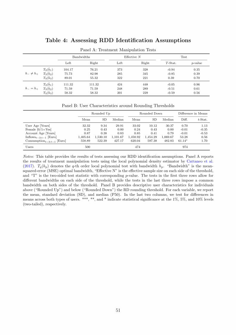
Table 4: Assessing RDD Identification Assumptions
Panel A: Treatment Manipulation Tests
Bandwidths Effective N Test
Left Right Left Right T -Stat. p-value
h− 6= h+
T2(h1) 104.17 76.21 373 328 -0.94 0.35
T3(h2) 75.73 82.98 285 345 -0.85 0.39
T4(h3) 89.01 55.32 322 221 0.39 0.70
h− = h+
T2(h1) 111.32 111.32 424 448 -0.05 0.96
T3(h2) 71.59 71.59 248 289 -0.51 0.61
T4(h3) 58.32 58.32 201 229 -0.59 0.56
Panel B: User Characteristics around Rounding Thresholds
Rounded Up Rounded Down Difference in Means
Mean SD Median Mean SD Median Diff. t-Stat.
User Age [Years] 32.32 9.34 29.91 33.02 10.12 30.37 0.70 1.13Female [0/1=Yes] 0.25 0.43 0.00 0.24 0.43 0.00 -0.01 -0.35Account Age [Years] 0.87 0.38 0.83 0.85 0.41 0.79 -0.01 -0.53Inflowst−3:t−1 [Euro] 1,405.64 1,530.10 1,101.67 1,458.92 1,454.29 1,069.67 53.28 0.56Consumptiont−3:t−1 [Euro] 558.89 522.39 427.17 620.04 597.38 482.83 61.14∗ 1.70
Users 500 474 974
Notes: This table provides the results of tests assessing our RDD identification assumptions. Panel A reportsthe results of treatment manipulation tests using the local polynomial density estimator by Cattaneo et al.(2017). Tq(hp) denotes the q-th order local polynomial test with bandwidth hp. “Bandwidth” is the mean-squared-error (MSE) optimal bandwidth, “Effective N” is the effective sample size on each side of the threshold,and “T” is the two-sided test statistic with corresponding p-value. The tests in the first three rows allow fordifferent bandwidths on each side of the threshold, while the tests in the last three rows impose a commonbandwidth on both sides of the threshold. Panel B provides descriptive user characteristics for individualsabove (“Rounded Up”) and below (“Rounded Down”) the RD rounding threshold. For each variable, we reportthe mean, standard deviation (SD), and median (P50). In the last two columns, we test for differences inmeans across both types of users. ***, **, and * indicate statistical significance at the 1%, 5%, and 10% levels(two-tailed), respectively.
51

Table 5: Consumption Growth around Rounding Thresholds
Dependent Variable (×100):Consumptiont+1:t+3−Consumptiont−3:t−1
Inflowst−3:t−1
(1) (2) (3) (4)
Conventional 17.63∗∗ 23.48∗∗ 17.96∗∗ 23.70∗∗
(2.19) (2.20) (2.12) (2.34)
Robust 21.56∗∗ 26.52∗∗ 21.83∗∗ 26.62∗∗
(2.37) (2.31) (2.31) (2.46)
Covariates No No Yes YesUser Observations 876 876 876 876Order Local Polynomial (p) 1 2 1 2Order Bias (q) 2 3 2 3Bandwidth Left 25.47 35.89 23.98 36.86Bandwidth Right 25.47 35.89 23.98 36.86
Notes: This table presents non-parametric estimates for the RD treatment effect of a 250 Euro higher overdraftamount on users’ consumption behavior. The dependent variable is the difference in average consumption threemonths before and after the treatment, normalized by the average account inflows three months prior to theoverdraft application. We residualize users’ consumption growth rate with country × year-month fixed effectsto ensure that we compare treated and control users from the same European country at a similar point intime. We only use polynomials of order 1 and 2 to avoid overfitting issues (Gelman and Imbens, 2018), applyweights from a triangular kernel because it is the mean squared error (MSE) minimizing choice (Cheng et al.,1997), and employ the MSE-optimal bandwidth selection procedure recommended by (Calonico et al., 2014).We report both conventional and robust RD estimates (Calonico et al., 2014, 2019). In columns (1) and (2),we do not add any covariates. In columns (3) and (4), we control for User Age, gender (Female), and AccountAge. ***, **, and * indicate statistical significance at the 1%, 5%, and 10% levels (two-tailed), respectively.
52

Appendix
Table A1: Variable Definitions
Variable Definition
Account Age End of month date minus the date when the user completed the account openingprocedure.
Card Consumption Total amount of electronic card consumption in the given month.Cash Withdrawals Total amount of cash withdrawals in the given month.Consumption Sum of Card Consumption and Cash Withdrawals.Deposits Total amount of available funds in a user’s account at the end of a month.Discretionary Sum of users’ monthly expenditures on Entertainment, Shopping, Gastronomy, and
Travel.Female Indicator variable equal to one if the user is female.Inflows Total amount of all incoming transactions a user receives in the given month.Urban Indicator variable equal to one if the user lives in a NUTS3 region with a population
of at least 500,000 people.Negative Deposits Indicator variable equal to one if the user has a negative account balance in the given
month.Non-Discretionary Card Consumption minus Discretionary spending.Overdraft Available Indicator variable equal to one if the user has access to a mobile overdraft in the given
month.Overdraft Amount Maximum overdraft amount granted to the user by the bank in the given month.User Age End of month date minus first day of user’s birth year.
53

Figure A1: Distribution of Forcing Variable around RoundingThresholds
Panel A: Histogram of Forcing Variable0
1020
3040
50Fr
eque
ncy
-100 -50 0 50 100Distance to Threshold
Panel B: Local Polynomial Density Estimate
00.0
02.0
02.0
04.0
04.0
06.0
06.0
08.0
08.0
1.0
1D
ensi
ty
-100-100 -50-50 00 5050 100100Distance to Threshold
Notes: This figure provides graphical evidence for our treatment manipulation tests in Section 6.3. Panel Aplots the number of users and Panel B reports the local polynomial density estimate by Cattaneo et al. (2017)for different values of our forcing variable Xi around the rounding threshold.
54

Figure A2: Robustness Analyses for Treatment Manipulation Tests
t = −1.645
t = 1.645
MSE Optimal Symmetric Bandwidth
−3
−2
−1
0
1
2
3
25 50 75 100 125Bandwidth
t−S
tatis
tics
Polynomial Order: p = 2 p = 3 p = 4
Notes: This figure reports t-statistics for the treatment manipulation test by Cattaneo et al. (2017) for differentpolynomial orders and bandwidth choices. The vertical horizontal lines indicate the critical 10% significancelevels at which the test rejects the null hypothesis that our running variable is locally continuous around therounding threshold.
55
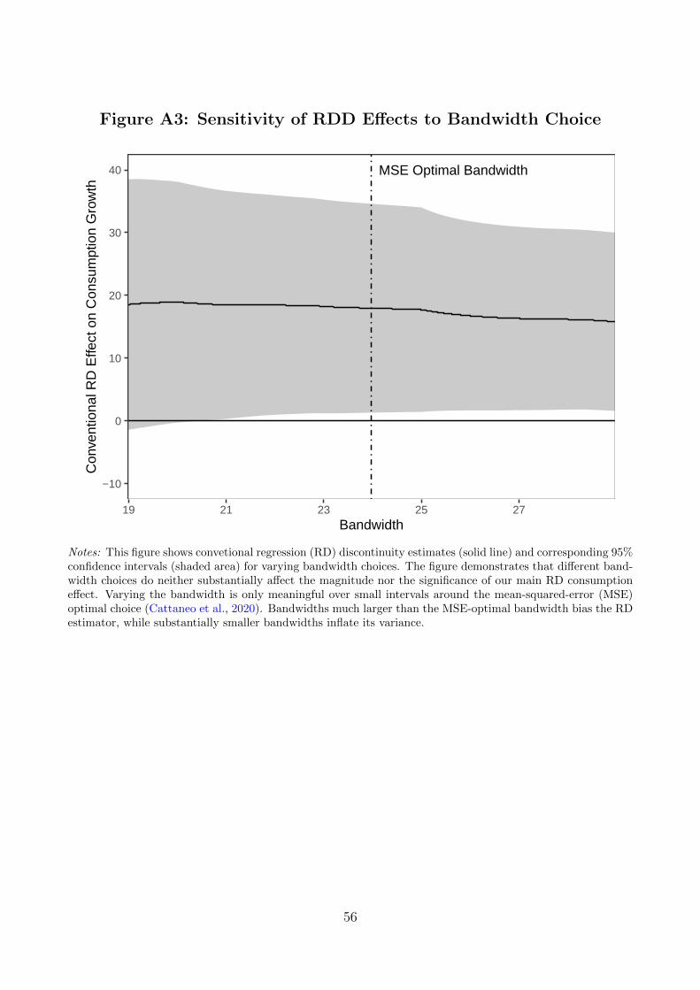
Figure A3: Sensitivity of RDD Effects to Bandwidth Choice
MSE Optimal Bandwidth
−10
0
10
20
30
40
19 21 23 25 27Bandwidth
Con
vent
iona
l RD
Effe
ct o
n C
onsu
mpt
ion
Gro
wth
Notes: This figure shows convetional regression (RD) discontinuity estimates (solid line) and corresponding 95%confidence intervals (shaded area) for varying bandwidth choices. The figure demonstrates that different band-width choices do neither substantially affect the magnitude nor the significance of our main RD consumptioneffect. Varying the bandwidth is only meaningful over small intervals around the mean-squared-error (MSE)optimal choice (Cattaneo et al., 2020). Bandwidths much larger than the MSE-optimal bandwidth bias the RDestimator, while substantially smaller bandwidths inflate its variance.
56
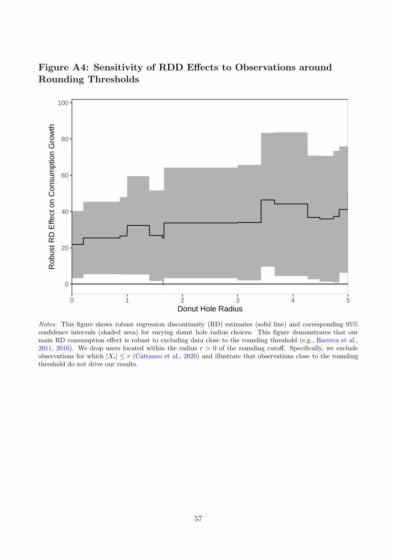
Figure A4: Sensitivity of RDD Effects to Observations aroundRounding Thresholds
0
20
40
60
80
100
0 1 2 3 4 5Donut Hole Radius
Rob
ust R
D E
ffect
on
Con
sum
ptio
n G
row
th
Notes: This figure shows robust regression discontinuity (RD) estimates (solid line) and corresponding 95%confidence intervals (shaded area) for varying donut hole radius choices. This figure demonstrates that ourmain RD consumption effect is robust to excluding data close to the rounding threshold (e.g., Barreca et al.,2011, 2016). We drop users located within the radius r > 0 of the rounding cutoff. Specifically, we excludeobservations for which |Xi| ≤ r (Cattaneo et al., 2020) and illustrate that observations close to the roundingthreshold do not drive our results.
57

Table A2: User Characteristics around Rounding Thresholds
Dependent Variable: User Age Female Account Age Consumption Inflows
(1) (2) (3) (4) (5)
Conventional 3.485 -0.00263 0.0568 -347.1∗ -535.2∗
(1.28) (-0.02) (0.61) (-1.82) (-1.84)
Robust 4.192 -0.0407 0.0432 -391.4∗ -554.4(1.26) (-0.24) (0.39) (-1.72) (-1.54)
Covariates No No No No NoUser Observations 972 972 972 972 972Order Local Polynomial (p) 1 1 1 1 1Order Bias (q) 2 2 2 2 2Bandwidth Left 29.77 33.95 41.64 39.81 31.04Bandwidth Right 29.77 33.95 41.64 39.81 31.04
Notes: This table reports non-parametric estimates for the RD treatment effect of a 250 Euro higher overdraftamount on several user characteristics. The dependent variables are the user’s age, gender, and time sinceaccount opening at the treatment date as well as the user’s level of consumption and inflows in the 3 months priorto the overdraft application. We only use polynomials of order 1 and 2 to avoid overfitting issues (Gelman andImbens, 2018), apply weights from a triangular kernel because it is the mean squared error (MSE) minimizingchoice (Cheng et al., 1997), and employ the MSE-optimal bandwidth selection procedure recommended byCalonico et al. (2014). We report both conventional and robust RD estimates (Calonico et al., 2014, 2019).***, **, and * indicate statistical significance at the 1%, 5%, and 10% levels (two-tailed), respectively.
58

Table A3: Survey Questions
Question Possible Answers
Do you rate yourself as a risk-taking person or areyou trying to avoid risks?
Scale from 0 (not willing to take risks) to 10 (verywilling to take risks)
Would you say that you are a person who trusts oth-ers, or not?
Scale from 0 (I do not trust others) to 10 (I trustothers fully)
When you make savings or investment decisions foryourself, which of the following statements describesyou best?
1 – I take significant risks and want to generate highreturns.2 – I take above-average risks and want to achieveabove-average returns.3 – I take average risks and aim for average returns.4 – I am not willing to take any financial risk andaccept not to generate any returns.
Imagine, you get either 100 Euros immediately or ahigher amount of money in a month. What is thelowest amount you would be willing to wait for amonth?
1 – 101 Euros2 – 103 Euros3 – 108 Euros4 – 117 Euros5 – 125 Euros6 – 133 Euros7 – 150 Euros8 – 167 Euros9 – 183 Euros10 – 200 Euros11 – 233 Euros
How likely is it that you will face large, unexpectedexpenses over the next 12 months?
Scale from 0 (very unlikely) to 10 (very likely)
How likely is it that you will face large medicalexpenses for yourself or a family member over thenext 12 months, including hospitalization and nurs-ing care?
Scale from 0 (very unlikely) to 10 (very likely)
How likely are you to lose your job in the next 12months?
Scale from 0 (very unlikely) to 10 (very likely)
How satisfied are you with your health at the mo-ment?
Scale from 0 (not satisfied) to 10 (very satisfied)
What do you usually think of when saving? 1 – I usually save for very specific expenses, such asa vacation or a car.2 – I usually save to have a small amount of moneyavailable for unexpected expenses.3 – I do not save much or cannot save much. When-ever I put money aside, I do it without much thought.4 – I am saving with the goal of building a small es-tate that I may pass on to my children, nephews,nieces, or other family members.
Suppose you have 100 Euros in your savings accountand earn 10 percent interest per year. How high willbe your balance after 2 years?
1 – Lower than 120 Euros2 – 120 Euros3 – Higher than 120 Euros
How high do you estimate your life expectancy? Enter number
59