working paper no. 12-11 g the sovereign spread in asian

Department of Economics and Finance

Working Paper No. 12-11

http://www.brunel.ac.uk/economics

Eco

nom

ics

and F

inance

Work

ing P

aper

Series

Sanjay Banerji, Alexia Ventouri and Zilong Wang

The sovereign spread in Asian emerging economies: The significance of external versus internal factors

September 2012

The sovereign spread in Asian emerging economies:

The significance of external versus internal factors

Sanjay Banerji†, Alexia Ventouri*, Zilong Wang‡

Abstract

This paper investigates the dynamic relations between external factors, domestic macroeconomic factors and sovereign spreads in Asian emerging countries. We conduct our analysis using a methodology that combines theoretical and empirical elements, using a Structural Vector Autoregression (SVAR) model. In particular, we investigate how the spread of sovereign debt is influenced over time by both external as well as domestic factors. Moreover, we generate variance decompositions and impulse response functions. Our results show that variations in sovereign spreads are mainly driven by external shocks, with the term structure of U.S. interest rate and the global risk aversion having the most important role. The findings also indicate that shocks from the U.S. have a direct effect on sovereign spread and an indirect effect via domestic macroeconomic fundamentals. Finally, the evidence produced validates the presence of some response patterns of sovereign spread to the external shocks.

Keywords: Bond spread; SVAR; Sovereign risk; Emerging market; Risk aversion

JEL classification codes: F34; F41; G15

*(Corresponding author): School of Social Sciences, Department of Economics and Finance, Brunel University, Uxbridge, UB8 3PH (United Kingdom); Tel: +44-1895-267165. Email: [email protected]. † Nottingham University Business School, University of Nottingham, Nottingham, NG8 1BB (United Kingdom); Tel: +44-1159-515276. Email: [email protected]. ‡ Essex Business School, University of Essex, Colchester, CO4 3SQ (United Kingdom); Email: [email protected].

1

mailto:[email protected]



1. Introduction

Since the 1990s, there is a significant increase in the amount of outstanding debt and by

2010, the world had over 77 trillion dollars aggregate outstand sovereign bond according

to BIS. Not only such bonds formed an important class of portfolio for investors, they

were also key source of funds for the Governments of the emerging markets. Hence,

understanding the factors behind the magnitude of spread and its volatility and how they

are influenced by foreign and domestic factors over time are important not only for the

purpose of inclusion in a well diversified portfolio but also for grasping its efficacy as a

financial instrument of the government in emerging economies. The sovereign spreads of

the U.S. Dollar denominated bond are typically defined as the difference in yield

between the bond and a benchmark U.S. Treasury bond of a similar maturity and are

normally expressed in basis point. The return on emerging market issues of such bonds is

in general expressed in terms of their spread rather than their absolute yield.

In this paper, we aim to assess the relative importance of both domestic and

external factors in influencing the variations of spread of the sovereign bonds issued by

the Asian emerging countries. In order to resolve endogeneity problems stemming from

the dynamic interdependence between these variables, we employ a Structural Vector

Autoregression (SVAR, hereafter) model. In addition, instead of following the traditional

approach relying on exchange rate, we use the U.S. Dollar index1 as a proxy for the

currency risk that affects the probability of default of sovereign bonds and their spread.

Based on this framework, results show that external factors cause variations of

both domestic macroeconomic variables (trade balance to GDP ratio and debt to GDP

ratio) and sovereign spreads. Moreover, there is evidence suggesting that external factors

1Dollar index is a trade-weighted average of six foreign currencies against the dollar. Currently, the index includes Euros (EUR), Japanese yen (JPY), British pounds (GBP), Canadian dollars (CAD), Swedish kronas (SEK) and Swiss francs (CHF).

2

not only directly affect sovereign spread, but indirectly causes fluctuation of sovereign

spread via its impact on the domestic macroeconomic fundamentals. Although the

evidence shows the indirect effects are limited, still we cannot ignore this fact.

This paper advances the previous literature in the following directions: Firstly,

one of the main advantages is that we explicitly take into account currency risk by

bringing the Dollar exchange rate into the analysis. The bulk of empirical evidence on

capturing currency risk tends to use the exchange rate between domestic currency and

the U.S. Dollar (treated as a domestic factor). However, currency risk can be seen as a

pure external factor, implying that the Dollar index can be used as a more appropriate

measurement to capture this fact. Specifically, the exchange rate can be affected by

domestic factors, such as high debt level etc. Yet, previous studies on this issue have

already included those variables in the model, which in turn implies that after controlling

for domestic macroeconomic fundamentals, exchange risk can be seen as a pure external

factor. A second advancement of this paper is that we investigate the dynamic role of

term structure of U.S interest rate on domestic economy and sovereign spread, most of

previous work focus on the spot U.S interest rate since their models are static. An

increase in the expected future short term U.S interest rate might cause a higher cost of

borrowing in emerging countries, but on the other hand it signals a recovery in a world

economy.

A third advancement of this paper is that we conduct our investigation using data

from Asian emerging markets. As far as we are aware, our study is the first to explore the

dynamic impact of debt on the sovereign spread, within the Asian market. Lastly, from a

methodological point of view, our approach considers the inclusion of two proxies for

the global risk aversion as determinants of the spread: (a) volatility risk, measured by

3

variance risk premium of the S&P 500; and (b) credit risk, based on the spreads on high-

yield BAA U.S. corporate bonds.

The role of sovereign bond spreads in emerging economies has generated a lot of

interest among economists for the best part of the past century. Edwards (1984) provides

a simple valuation framework for the determination of emerging market sovereign bonds

under the assumption that investors are risk neutral. The analysis is based on a sample of

19 developing countries over 1976-1980. Using random effects components estimation,

he provides evidence suggesting that the spread is determined by the reserves-to-GNP,

debt-to-GDP and Debt-service ratios, as well as by the propensity to invest. Based on the

same methodology, Arora et al. (2001) investigate the impact of changes in the U.S.

monetary policy on country risk and economic growth in several developing countries in

Latin America, Asia, and Eastern Europe over the period 1994-1999. The results indicate

that the level of U.S. interest rates has a direct positive effect on sovereign bond spreads.

The findings also document that country risk (proxied by sovereign bond spreads) is

influenced by the U.S. monetary policy, the country-specific fundamentals, and the

conditions of the global capital markets.

Diaz and Gemmill (2006) use end-of-month market prices of Par Brady bonds to

investigate the impact of global, regional and country-specific factors on the

creditworthiness of four emerging countries. The time span considered is from April

1994 to October 2001. The results document that credit risk (as measured by the

estimated distance-to-default) is mainly driven by systematic global and regional factors,

implying that credit risk should be treated as non-diversifiable. Thus, their result tend to

suggest that credit ratings for those emerging markets should be based more strongly on

global and regional economic factors than on local factors. One notable result which

relate to this paper is that they use term structure of U.S interest rate as an explanatory

4

variable, it has significant positive effects on the distance-to-default, but when the on

period lag of the term structure of U.S. interest rate takes into account, the effects

disappear in Brazil and Mexico.

The abovementioned studies rely on OLS and panel regressions to investigate the

relationship between sovereign spread, credit ratings and macroeconomic variables.

More recently, studies have turned their attention to the endogeneity of sovereign spread

and the role of risk aversion. More specifically, two strands of literature have emerged as

the most prominent in the field of sovereign spread. One investigates the interaction of

sovereign spread with domestic business cycles. A second strand of literature has

engaged in examining the impact of risk aversion on sovereign spread.

Uribe and Yue (2006) examine the interaction of sovereign spreads, the world

interest rate, and business conditions in emerging markets. Using a panel VAR model,

the authors find that sovereign spreads affect aggregate activity, but, interestingly, at the

same time respond to domestic macroeconomic conditions. Even more importantly, their

findings highlight the issue of sovereign spreads and their dependence on domestic

fundamentals and the world interest rate appear to be of great interest in understanding

business cycles in emerging countries. However, this analysis does not take into account

the role of global risk aversion, which may also affect sovereign spreads, especially in an

open emerging market economy.

The novelty of the second strand of literature is that it explicitly investigates risk

aversion and its impact on sovereign spread (Blanchard, 2005). Dungey et al. (2004) use

SVAR to explore the role of investor' risk aversion during three financial crisis period

(Russian crisis, LTCM crisis and Brazilian crisis). Their results suggest that the increase

in the sovereign spread in most of the countries during Russian and LTCM crisis is

mainly caused by credit risk and country risk, whereas during Brazilian crisis period, the

5

increase in sovereign spread is driven by credit, liquidity and volatility risk. Garcia-

Herrero and Ortiz (2006) use a four variables SVAR model to identify the underlying

foreign determinants of Latin American sovereign spreads. Their findings suggest that

U.S. growth and interest rate have a direct effect on sovereign spread and an indirect

effect on global risk aversion. Yet, the issue of endogeneity is not explicitly captured by

this model. In a more recent study, Fracasso (2007) attempts to fill this gap in the

literature by considering both the endogeneity of the credit spreads and relate them to the

degree of risk aversion of international investors, as well as to domestic and international

macroeconomic factors. 2 The analysis is based on a VAR system encompassing six

domestic and three foreign variables3 capturing global factors in Brazil during 1999-

2004. The evidence broadly supports the view that foreign factors, in particular global

appetite for risk and global risk aversion, are important determinants of the development

of the domestic variables.

Finally, Eichler and Maltritz (2012) examine the determinants of the government

bond yield spread of EMU member across different maturities. Using a panel regression,

the authors find that both economic growth and countries' openness are significant

determinants of government bond yield spread for all maturities. The countries' debt to

GDP ratio is only significant for short term government bond yield spread, whereas net

lending, interest rate costs and trade balance are significant for long term government

bond yield spread.

Overall, understanding these relationships has important policy implications as

researchers should take into account both domestic and external factors, as well as the

role of global risk aversion, when investigating emerging economies. Although several

2The focus of this study is to examine the impact of foreign global shocks on the behaviour of domestic macroeconomic variables (in particular external debt and EMBI spread) in Brazil. 3 The author uses the industrial cycle; primary deficit; real depreciation; inflation; external debt; and EMBI spread as domestic variables while the US industrial cycle; US Federal fund rate; US-BAA corporate high yield spread are used as foreign variables.

6

studies have investigated sovereign spread in emerging markets, none of them offer

explicit consideration of foreign and domestic factors in determining the shapes of the

spread over time. Table B in the Appendix B presents a summary of the previous studies

on sovereign spread, along with their main findings. On balance, the existing literature

indicates that foreign and domestic factors can significantly influence sovereign spread.

The remaining of the paper is organized as follows: Section 2 develops the

theoretical model. Section 3 presents the data and variables. Section 4 presents the

estimation strategy of a SVAR model. Section 5 discusses the empirical results for the

variance decomposition and impulse response functions, and Section 6 concludes.

2. Theoretical model

In order to show interdependence between various variables, we resort to a simple

framework that combines an incentive model of debt overhang (Obstfeldt and Rogoff,

1996; chapter 6) with a framework by Blanchard (2005) who analyzed capital inflow,

debt and default in the context of a portfolio allocation model.

We consider a one period model with two risk averse representative investors: An

emerging market investor whom we call the Malaysian investor and international

investor. There are three assets: 1) A risk free one-period Malaysian bond denominated

in domestic currency with rate of return r. 2) A one-period Malaysian government bond

denominated in U.S. dollar with rate of return MAr , let p be the probability of default on

Malaysian government bond. 3) A risk free one-period U.S. government bond

denominated in U.S. dollar with rate of return . We also assume that there are some

capital flow restrictions: 1) Malaysian investor can only buy Malaysian risk free bond

and Malaysian government’s U.S. dollar bond; 2) International investor can only buy

U.S. government’s bond and Malaysian government’s U.S. dollar bond.

USr

7

2.1. Portfolio allocation model

Consider the Malaysian investor with initial endowment W and invest x amount on

Malaysian risk free bond, then her utility is:

'( (1 )) (1 ) ( (1 ) ( ) (1 ))MApU x r p U x r W x rεε

+ + − + + − + (1)

By the expected utility theory, we can rewrite equation (1):

'{ (1 )) (1 )[ (1 ) ( ) (1 )] [( ), , ]}MAU px r p x r W x r f W x pε θε

+ + − + + − + − − (2)

where ε is the real exchange rate measure by domestic good per foreign good,

primes denote next-period variables, f is the premium that agents willing to pay to get a

certain payment, θ measure the degree of risk aversion and f is a function of W-x, θ and

p. We assume f is a linear function of W-x, θ and p and

( )f W x pθ= − , then rewrite (2)

'{ (1 ) (1 )( ) (1 )] ( ) ]}MAU x r p W x r W x pε θε

+ + − − + − − (3)

Maximise (3) respect to x:

'(1 ) (1 ) (1 )MAp r r pε θε

− + = + + (4)

Using same methodology for international investor:

(1 )(1 ) (1 ) *MA USp r r θ− + = + + p (5)

where θ* is the degree of risk aversion of international investor.

8

2.2. Capital flows and debt dynamic

Since international investor choose between Malaysian government U.S. dollar bond and

U.S. government bond, rewrite equation (5) in terms of Malaysian good:

' '(1 ) (1 ) (1 ) *MA USp r r pε ε θε ε

− + = + +

Capital flows are given by:

' '{(1 ) (1 ) (1 ) * } ' 0MA USCF C p r r p Cε ε θε ε

= − + − + − >

Use equation (4),

'{1 (1 ) ( *) }USCF C r r pε θ θε

= + − + + −

Assume there is home bias, so international investors are more risk averse than

Malaysian investor, which in turn θ*>θ. We further assume

*, 1θ λθ λ= ≤

then capital flow are given by:

'{1 (1 ) (1 ) * }USCF C r r pε λ θε

= + − + − −

Assume the net exports are a function of the real exchange rate:

( ) '( ) 0NX N Nε ε= >

In the equilibrium condition, the sum of the capital flow and the net exports has to be

zero gives:

'{1 (1 ) (1 ) * } ( ) 0USC r r p Nε λ θ εε

+ − + − − + =

Since this is a one-period model, we normalize the long run equilibrium exchange rate to

be equal to one, then assume

' , 0 1ηε ε η= ≤ ≤

9

replacing 'ε in the equilibrium condition:

1{1 (1 ) (1 ) * } ( ) 0USC r r p Nηε λ θ−+ − + − − + =ε (6)

The equation (6) determines the exchange rate as a function of p the

probability of default. Consider the Malaysian government inherited an outstanding

amount of U.S. dollar debt D$, then the debt at the start of next period is given by:

$' (1 ) 'MAD r D Rε= + −

where, R is the primary surplus, D' and R are measured in Malaysian goods.

Use equation (5)

$1 *' ( )1 1

USr pD D Rp p

ηθ ε+= +

− −− (7)

The equation (7) gives a relationship between D and p. The debt in the next period

depends on the probability of default directly as well as via exchange rate

from the equilibrium condition (6).

2.3. Incentive model

The Malaysian government needs to repay D' in the second period and there are two

output states in the second period, good state output YG and bad state out YB. We further

assume that YG>D'> YB, and in the bad state, the Malaysian government default and pays

nothing to the bond holder. The state depends on the Malaysian government's effort e,

hence the probability of the default depends on Malaysian government's effort, and there

is a dislike of effort, then the cost of effort is φ(e), where e is continuous, φ() is a convex

function with φ(0)=0, φ’(0)=0 and φ(1)=+∞. In order to simplify the problem, we assume

that p(e)=1-e and φ(e)= 0.5me2, this assumption does not affect our results. The

Malaysian government maximizes its utility:

2( ') (1 ) ( ) 0.5G BeU Y D e U Y me− + − −

10

By first order condition:

( ') ( )G BU Y D U Y me− − =

Replacing e with 1-p:

( ') ( ) (1G BU Y D U Y m p− − = − ) (8)

The equation (8) and (7) determine the equilibrium p and D' together, as a function of

risk aversion parameter, GDP and other variables. By implicit function theorem, the

following comparative statics are computed (see for more details Appendix A):

' '0, 0, 0* *US

D D prθ θ

∂ ∂ ∂> >

∂ ∂ ∂> and 0US

pr∂

>∂

Define the sovereign spreads as the rate of return difference between the Malaysian

government U.S. dollar bond and the U.S. government U.S. dollar bond, rearrange (5):

(1 *)1

MA US US pS r r rp

θ= − = + +−

2

1(1 *)1 (1

USUS US

S p rr p p

θ∂ ∂= + + +

)p

r− ∂∂ −

2

1(1 *)* 1 (1 ) *

USS p rp p

θ pθ θ∂ ∂

= + + +∂ − − ∂

The first term in the above two equations is the direct effects of U.S. interest and

international risk aversion on sovereign spread, whereas the second term is the indirect

effects via probability of default.

To summarize, we can construct the following hypothesis:

1. If there is an unexpected increase in the U.S. interest rate, there will be an increase in

the emerging countries' debt level, probability of default and sovereign spread.

2. If there is an unexpected increase in the international investors' risk aversion, there

will be an increase in the emerging countries' debt level, probability of default and

sovereign spread.

11

Given that the estimation of the above model reveals a complicated equilibrium

relationship between sovereign spread, domestic and external factors, we use a SVAR,

model. This method allows for valid inference and resolves the endogeneity problem

that seems to plague our estimations.

3. Data and variables

This study uses a SVAR model to study the relative contribution of external and internal

variables to the volatility of macroeconomic variables and credit spread. In order to

account for the endogeneity of sovereign spread and risk aversion, we include the

following sets of foreign (external) and domestic (internal) variables:

FOREIGN = (TERM STRUCTURE, CBS, VRP, DOLLAR) (9a)

DOMESTIC = (TRADE/GDP, DEBT/GDP, LOGSPREAD) (9b)

The vector FOREIGN (equation 9a) includes four sets of external variables: the

term structure of the U.S. interest rate (TERM STRUCTURE); the U.S.-BAA corporate

bond spread (CBS); the variance risk premium (VRP) and the Dollar Index (DOLLAR).

Similarly, the vector of domestic variables (DOMESTIC) in equation (9b) contains the

trade balance to GDP ratio (TRADE/GDP); the debt to GDP ratio (DEBT/GDP) and the

LOGSPREAD, as measured by the log to the level of EMBI global index.

In particular, we control for the future short term interest rate and prospect of

future U.S. economy by using the term structure of the U.S. interest rate. To account for

global risk aversion we use two proxies: the U.S.-BAA spread (CBS) and the variance

risk premium (VRP). The Dollar index is used as a proxy of the real value changed of

Dollar. Turning to the variables capturing the domestic factors, we use the trade balance

12

to GDP ratio (TRADE/GDP) as a proxy for domestic liquidity condition and debt to

GDP ratio (DEBT/GDP) as a proxy for the domestic solvency condition. Both variables

have been identified as important determinants of the emerging market sovereign spreads

(see among others, Min, 1998; Arora et al., 2001; Eichler and Maltritz, 2012). Finally,

the LOGSPREAD variable is a measure of the cost of borrowing. Table 1 provides

detailed information on the variables employed in the model.

<Insert table 1 about here>

The sovereign spread of a U.S. Dollar denominated bond is defined as the

difference in yield between the bond and a benchmark U.S. Treasury bond of a similar

maturity, and is normally expressed in basis point. The return on emerging market issues

is expressed as their spread rather than their absolute yield (LOGSPREAD). This study

uses the J.P. Morgan EMBI Global spread index as a proxy of sovereign spread for

different countries. The EMBI Global is a weighted average of the spreads of U.S.

Dollar-denominated individual bonds issued by a particular emerging market country.4

The EMBI Global controls for floating coupons, principal collateral, rolling interest

guarantees, and other unusual features of the bonds, and it is computed for all the main

emerging market sovereign issuers, which also allows direct comparability of the results

across countries in the sample.

The dataset used in this study is composed of different sample periods for each

country under investigation.5 In particular, and due to the data availability,6 the chosen

4 Other studies (e.g. Dungey et al., 2004) use a benchmark bond for each country to define the spread. However, and given that the purpose of this study is to look at the spread related to the risk of a sovereign issuer rather than the spreads of individual bonds, the EMBI Global is considered more appropriate for this type of investigation. 5 We choose the largest time span possible.

13

time span per country is as follows: Chinese data are from Jan. 1995 to Sep. 2009;

Malaysian data are from Nov. 1996 to Sep. 2009; Philippine data are from Jan. 1998 to

Sep. 2009; and finally Indonesian data are from Jun. 2004 to Sep. 2009. For similar

reasons, when only quarterly and yearly data are available, 7 we convert the

corresponding series to monthly frequency. Table 2 presents the full raw data

information.

<Insert Table 2 about here>

Table 3 presents the summary statistics for the variables employed in the model

per country. China presents the lowest mean value of sovereign spread and debt to GDP

level...On the other hand, Philippines has the highest mean value of sovereign spread and

debt to GDP level. Malaysia presents the highest mean value of trade balance to GDP

ratio, whereas Indonesia has the lowest trade balance to GDP ratio. By ranking the mean

value of the DEBT/GDP ratio, Philippines represent the largest group, followed by

Indonesia, Malaysia and China. Table 3 also presents the results after checking for

stationarity. The unit root tests we ran include the Augmented Dickey Fuller (ADF Tests)

and the Kwiatkowski, Phillips, Schmidt and Shin (KPSS tests). According to both tests,

the CBS, DOLLAR and DEBT/GDP variables are I(1) stationary, with the remaining

ones being I(0) stationary. For that reason, CBS, DOLLAR and DEBT/GDP variables

are measured by taking the difference of their logs.


6Since the information on the J.P. Morgan EMBI Global index is not available for all countries and years, we construct our analysis based on the available data. 7This is due to the fact that data for the debt level in China are available in years.

14

4. The empirical model

To test the dynamic relations between sovereign spread, domestic macroeconomic

variables and external factors we use a SVAR method as our modeling framework. This

method allows us to generate an impulse response function, which simulates the effects

of a shock to one variable in the system on the conditional forecast of another variable.

In this context, the application of a SVAR model allows us to obtain the variance

decomposition, which determines how much of the forecast error variance of each of the

variables can be explained by exogenous shocks to the other variables. Finally, we also

compare the short-term and the long-term effects. Specifically, we estimate the following

econometric model that constructs impulse response function and variance

decomposition:

1 1 ...t t p t p tAY AY A Y Bα ε− −= + + + (10)

where, A represents a matrix of instantaneous relations between the variables in

Y; B is a matrix of contemporaneous relationships among the structural disturbances ε

and p is the period of lag. The vector Yt in the model contains the set of external and

internal variables as specified in equations (9a and 9b). Therefore, equation (10) can be

re-written as follows:

1

1

1

1 1

1

1

1

.../ // /

t t

t t

t t

t t p

t t

t t

t t

TERM STRUCTURETERM STRUCTURE TERM STRUCTURECBS CBSVRP VRP

A DOLLAR A DOLLAR ATRADE GDP TRADE GDPDEBT GDP DEBT GDPLOGSPREAD LOGSPREAD

−

−

−

−

−

−

−

⎛ ⎞ ⎛ ⎞⎜ ⎟ ⎜ ⎟⎜ ⎟ ⎜ ⎟⎜ ⎟ ⎜ ⎟⎜ ⎟ ⎜ ⎟

= +⎜ ⎟ ⎜ ⎟⎜ ⎟ ⎜ ⎟⎜ ⎟ ⎜ ⎟⎜ ⎟ ⎜ ⎟⎜ ⎟ ⎜ ⎟⎝ ⎠ ⎝ ⎠

//

t p

t p

t p

t p t

t p

t p

t p

CBSVRP

DOLLAR BTRADE GDPDEBT GDPLOGSPREAD

ε

−

−

−

−

−

−

−

⎛ ⎞⎜ ⎟⎜ ⎟⎜ ⎟⎜ ⎟

+⎜ ⎟⎜ ⎟⎜ ⎟⎜ ⎟⎜ ⎟⎝ ⎠

15

In order to estimate the SVAR model, two issues have to be considered: impulse

restrictions and autocorrelation. In particular, the solution of the SVAR model involves a

number of restrictions that have to be implemented. That is, given that the U.S. market is

a large, integrated financial centre, this implies that the U.S. Dollar and U.S. investors

play a very important role in the global financial market. As such, we implicitly assume

that the U.S. variables are appropriate proxies of global factors, and that all the U.S.

variables should be treated as exogenous ones. We adopt this restriction because it is

reasonable to assume that the U.S. variables may affect, but not be affected by the

domestic ones.

An additional restriction we impose in estimating the SVAR system is that the

TERM STRUCTURE variable is non- contemporaneous and unaffected by any other

variables. The TERM STRUCTURE has a contemporaneous effect on CBS and VRP,

but CBS and VRP do no contemporaneously affect each other. Alternatively, the TERM

STRUCTURE, CBS and VRP have a contemporaneous effect on the DOLLAR. In

addition, all the external variables have a contemporaneous effect on TRADE/GDP,

while the DEBT/GDP is contemporaneously affected by the external variables and the

TRADE/GDP. Finally, all variables have contemporaneously effect on sovereign spread.

Another important issue for the estimation of the SVAR model is to address for

autocorrelation. In order to make sure no autocorrelation appears in the error term after

estimation, a sufficient number of lags have to be employed. We first select for the

appropriate lag length using the Akaike Information Criterion (AIC) and the Hannan-

Quinn Information Criterion (HQIC). Following this methodology, we ending up with 14

lags for Malaysia, China and Philippines, and 5 lags for Indonesia.

16

5. Empirical results

This section first evaluates the empirical results for the variance decomposition analysis

(Section 5.1). Then, it discusses the results deriving from the impulse response function

of the variables employed in the VAR system (Section 5.2).

5.1 Variance decomposition analysis

To consider the contribution of the various shocks in the empirical model, we perform a

variance decomposition of the variables contained in the VAR system at different

horizons. Specifically, we focus on the fraction of the variance of the forecasting error

explained by each shock.

<Insert Table 4 about here>

Table 4 presents the contribution of all variables to the forecasting error variance

of sovereign spread. The column aggregate foreign factor is the sum of the TERM

STRUCRURE, CBS, VRP and DOLLAR variables. At 24 months horizon, foreign

shocks could explain 64%, 71%, 53% and 58% fluctuation in LOGSPREAD in Malaysia,

Indonesia, China and Philippines accordingly. The longer the horizon is, the greater the

effect of foreign shocks. The TERM STRCURE shock appears to be the most important

driven factor for LOSGPREAD, especially in the medium run between 6 and 18 months

horizon. Focusing on the different variables capturing risk aversion, credit risk (CBS)

appear to be more important than volatility risk (VRP), however they present different

explanatory patterns. That is, CBS shocks have great impact on fluctuation of

LOGSPERAD in the short run, but gradually lose its explanatory power, except for the

17

case of Indonesia. On the other hand, VRP shocks have limited effect on LOGSPREAD,

in the short run, while this effect increases the larger the horizon gets.

As far as the internal variables are concerned, the explanatory power for the

internal factors is under 10%, on average. This result implies that the domestic shocks

have limited effects on the fluctuation of LOGSPREAD. Interestingly, the results for

Philippines indicate that the DEBT/GDP shock can explain about 20% variation of

LOGSPREAD at 1 month horizon, but its effect disappears later on, while the

TRADE/GDP shock has almost no effects on the variation of LOGSPREAD, but pick up

at medium run, after 12 months horizon. This result indicates that policy makers should

always counteract unexpected changes in U.S. factors since they affect LOGSPREAD at

most either in medium or long run.


Table 5 reports the results for the contribution of U.S. variables to the forecasting

error variance of TRADE/GDP ratio. Overall, Aggregate foreign shocks could explain

55%, 70%, 45% and 69% of fluctuations in TRADE/GDP in Malaysia, Indonesia, China

and Philippines at 24 month horizon. Table 6 analyses the contribution of U.S. variables

to the forecasting error variance of debt to GDP ratio. Overall, aggregate foreign shocks

could explain 55%, 66%, 54% and 54% of fluctuations in DEBT/GDP in Malaysia,

Indonesia, China and Philippines, at 24 month horizon. Unexpected FOREIGN shocks

could explain large amounts of fluctuation in domestic macroeconomic fundamentals,

while the longer the horizon is, the larger the effect. This finding is in line with previous

findings (Fracasso, 2007).

18


In summary, foreign shocks could explain 50-70% the variation of domestic

variables, in particular, the TERM STRUCTURE shock could explain about 20%, which

is line with previous findings (Uribe and Yue, 2006). Our results also indicate that risk

aversion shocks could explain 20-40% variation of domestic variables. This result

corresponds to previous findings in the literature (Garcia-Herrero and Ortiz, 2006).

Finally, the DOLLAR shock could explain 10% variation of domestic variables. This is

also in line with previous findings in the literature (Fracasso, 2007). Furthermore,

domestic variable shocks could explain part of fluctuation in LOGPREAD. The next step

is to examine whether LOGSPREAD shock can also drive domestic variables. Table 7

reports the results from the contribution of sovereign spread to the forecasting error

variance of TRADE/GDP and DEBT/GDP. LOGSPREAD shock could explain about

10% variation of TRADE/GDP and DEBT/GDP. This result also in line with previous

findings provided by Uribe and Yue (2006), who suggest that sovereign spread shock,

can explain about 12% of movements in domestic economic activities.


5.2. Impulse response analysis

This section analysis the impulse response pattern of the variables employed in the VAR

system at different horizons. To recall, the SVAR method allow us to generate the

impulse response function, which simulates the effects of a shock to one variable in the

system on the conditional forecast of another variable. In that way, we attempt to further

investigate the response pattern of the various shocks in the empirical model. Given that

19

our findings suggest that domestic factors have no affect on the variation of sovereign

spread, the analysis for the domestic variable shocks are not presented in the paper.8

<Insert figure 1 about here>

Figure 1 illustrates the impulse response of sovereign spread to U.S. variable

shocks. The figure shows that if there is one unit of unexpected increase of one variable,

how other variables changes over the next 24 months. The solid line depicts point of

estimate of impulse response, and the dotted lines depict 95% confident interval. Overall,

the results in Figure 1 are consistent for all countries except the response pattern for VRP

shock, an ambiguous result given that the 95% confident interval includes zero. The

LOGSPREAD displays an increasing trend whenever there is a positive shock on the

TERM STRUCTURE, CBS or the DOLLAR index. This increasing affect continues

until the 3-6 months horizon, and then the response patterns are ambiguous, since the

shaded area is 95% confident include zero. The response of the risk aversion shocks are

in line with Garcia-Herrero and Ortiz (2006) who found a positive relationship between

risk aversion and sovereign spread. The result of the TERM STRUCTURE shock is quite

interesting, suggesting that if there is a shock of increasing expected future U.S. short

term interest rate, the present LOGSPREAD would go higher. This result suggest that

when the U.S feudal reserve use QE (quantitative easing) or operational twist, which

causes decline of the term structure of U.S interest rate, the countries in our sample

would benefit from those U.S monetary policy and incur a lower cost of sovereign

borrowing. This result is in line with Diaz and Gemmill (2006) who suggest the default

probability has positive relationship with the Term structure of U.S. interest rate.

8 The figures for the domestic variable shocks are not reported but are available with the authors upon request.

20

6. Conclusion

This paper contributes to the existing literature by analyzing the dynamic relations

between external factors, domestic macroeconomic factors and sovereign spreads in

Asian emerging countries. Our analysis includes a theoretical framework that combines

an incentive model of debt overhang (Obstfeldt and Rogoff, 1996; chapter 6) with

Blanchard (2005)’s who analyzed capital inflow, debt and default in the context of a

portfolio allocation model. Then we use a SVAR model to empirically investigate how

the spread of sovereign debt is influenced over time by both external as well as domestic

factors. In addition, using the estimated SVAR, we generate variance decompositions

and impulse response functions. One feature of this paper is that we explicitly take into

account currency risk by bringing the Dollar index into the analysis. Another important

advancement is the use of two global risk aversion proxies, namely volatility and credit

risk, as external factors. Those variables play an important role in both domestic

macroeconomic factors and sovereign spread. Finally, the present study attempts to shed

more light in an area that has not been extensively examined, such as the Asian emerging

market.

By combining the term structure of the U.S. interest rate, the BAA corporate

bond spread, the variance risk premium and the Dollar index as external factors, our

findings indicate that the variation of sovereign spreads in Asian emerging countries is

mainly driven by external shocks, with the term structure of U.S. interest rate and the

credit risk aversion playing the most important role. Moreover, we find that shocks from

the U.S. could largely explain fluctuations in domestic macroeconomic fundamentals,

implying that Asian economies are heavily rely on U.S. factors. This in turn implies that

the U.S. variables have a direct effect on sovereign spread and an indirect effect via

domestic macroeconomic fundamentals. Our findings also validate the presence of some

21

response patterns of sovereign spread to the external shocks. Sovereign spreads increase

the response to all kinds of external shocks.

From a public policy perspective, understanding the relationships among foreign,

domestic factors and sovereign spread is important for both investors and policy makers

alike, in deciding a suitable investment or government policy, especially in emerging

economies. Furthermore, our evidence highlights the crucial role of sovereign bond in

Asia, which is mainly driven by the U.S. economy. Asian economies appear to be

heavily depending on U.S., which in turn implies that when a shock is coming from the

U.S., its affect can be continuous in the medium and long run.

Yet there is no doubt that the recent financial markets turmoil puts this

discussion on a new basis. Further research could focus on the role of risk aversion

under different economies characteristics, e.g. under different exchange rate regime or

under different macroeconomic fundamental, those results would give policy maker

more insight on the best strategy to response for risk aversion shocks.

22

REFERENCES

Arora, V. and M. Cerisola, (2001), “How does U.S. monetary policy influence

sovereign spreads in emerging markets?” IMF Staff Papers, Vol. 48, pp. 474-498.

Blanchard, O., (2005), “Fiscal Dominance and Inflation Targeting. Lessons from

Brazil”, In Giavezzi, F., Goldfajn I. and S. Herrera (Eds.), Inflation Targeting,

Debt, and the Brazilian Experience, 1999 to 2003, Cambridge: MIT Press.

Diaz, W.D and G. Gemmill, (2006), “What drives credit risk in emerging markets? The

roles of country fundamentals and market co-movements” Journal of International

Money and Finance, Vol. 25 (3), pp.476-502.

Dungey, M., Fry, R., González-Hermosillo, B. and V. L. Martin, (2004),

“Characterizing Global Investors’ Risk Appetite for Emerging Market Debt during

Financial Crises”, IMF Working Paper, No. 03/251.

Edwards, S., (1984), “LDC Foreign Borrowing and DEFAULT Risk: An Empirical

Investigation 1976-1980”, American Economic Review, Vol. 74, pp.726-734.

Eichengreen, B. and A. Mody, (1998), “What explains changing spreads on emerging-

market debt: fundamentals or market sentiment?”, NBER working paper, No 6408.

Eichler,S. and D. Maltritz, (2012), “The term structure of sovereign default risk in EMU

member countries and its determinants”, Journal of Banking & Finance,

Forthcoming.

Fracasso, A., (2007), “The role of foreign and domestic factors in the evolution of the

Brazilian EMBI spread and debt dynamics”, HEI Working Paper No: 22/2007.

Garcia-Herrero A. and A. Ortiz, (2006), “The role of global risk aversion in explaining

Latin American sovereign spreads”, Economía, Vol. 7 (1), pp. 125-155.

Grandes, M., (2003), “Convergence and Divergence of Sovereign Bond Spreads:

Theory and Facts from Latin America”, Paris, France: Delta, ENS/EHES.

23

http://papers.ssrn.com/sol3/cf_dev/AbsByAuth.cfm?per_id=578493

Min, Hong G., (1998), “Determinants of Emerging Market Bond Spread: Do Economic

Fundamentals Matter?”, Policy Research Working Paper No. WPS 1899, The

World Bank, Washington D.C.

Sims, C., J. Stock, and M. Watson, (1990), “Inference in linear time series models with

some unit roots,” Econometrica, Econometric Society, Vol. 58 (1), pp. 113-144.

Sims, C., (1980), “Macroeconomics and reality”, Econometrica, Economometric

Society, Vol.48 (1), pp.1-48.

Obstfeld, M, and K. Rogoff, (1996), Foundations of international macroeconomics,

Cambridge MA: MIT Press.

Uribe, M. and V.Z. Yue, (2006), “Country spreads and emerging countries: who drives

whom?”, Journal of International Economics, Vol. 69 (1), pp. 6-36, and NBER

Working Paper 10018.

Zhou, H., (2010), “Variance Risk Premia, Asset Predictability Puzzles, and

Macroeconomic Uncertainty”, Finance and Economics Discussion Series, 2010-14,

Board of Governors of the Federal Reserve System (U.S.).

24

http://ssrn.com/abstract=1400049

http://ssrn.com/abstract=1400049

Appendix A: Theoretical model statics

From equilibrium condition (6)

11 {1 (1 ) (1 ) * } ( ) 0USF C r r p Nηε λ θ−= + − + − − + =ε (6)

By using implicit function theorem:

1

21

(1 ) * ' 0( 1) (1 ) ' 'US

FCp

Fp rη

ε λ θη ε

ε

−

∂∂ − −∂= − = − >

∂∂ − − + +∂

C N

Recall equilibrium condition (7) and (8)

$1 *' ( )1 1

USr pD Dp p

ηθ ε+= +

− −R−

)

(7)

( ') ( ) (1G BU Y D U Y m p− − = − (8)

(7) (8)

p

D’

Second order condition for (7) and (8)

$ $$ 1

2

1 * 1 *1 ' [( ) ( ) ](1 ) 1 1 1 1

US USUSr r p D pDdD D dp dr d

p p p p p

η ηη ηθ θ ε ε *

pεε η ε −+ + + ∂

− + + = +− − − ∂ − −

θ

*

' ' 0 0USU dD mdp dr dθ− + = +

25

Since the above graph shows that the equilibrium can only exist if the gradient of (7) is

smaller than (8), then the Jacobian determinant has to be bigger than zero.

The Jacobian determinant is

$

11

' 0

D

U−

−

$$ 1

2 $

1 * 1 *[( ) ( ) ]1 (1 ) 1 1

0' 1 0

US US

US

D r r pDp p p p p Dm

mD pr J J

ηη η

η

ε θ θ εε η εε

−+ + + ∂− + +− − − − ∂

∂ −= = >∂

26

$ 12

1 * 1 *1 [( ) ( ) ]0(1 ) 1 1

'

US USr r pDJ p p p p

U m

η ηθ θ εε η ε −+ + + ∂− + +

= >− − − ∂−

$

21 * 1 *[( ) ) ]

1 (1 10' 1 0

*

US USpD r r pDp p p p p pDm

D pJ J

ηη η

η

ε θ θ εεε

θ

−+ + + ∂+− − − ∂

∂ −= = >∂

$ 1

$

$

$1

1'

' 0 1 0*

pDp pDU

Up pJ J

η

η

εε

θ

−−∂ −= = >

∂

$

'1 0US

p DUp p

r J J

η

η

εε

∂ −= = >∂

() 1

m

ε η− +−

Appendix B

Table B

Selected Studies on Sovereign Spread

Author (publication date)

Period under study

Sample Methodology Main Findings

Edwards (1984)

1976-1980 727 public and publically guaranteed Eurodollar loans

Panel regression Spreads are determined by the debt to GNP and the dept service rations, as well as by the propensity to invest.

Min (1998)

1991-1995 11 Emerging countries

Panel regression Spreads are determined by the debt-to-GDP, reserves-to-GDP and debt-service-to exports ratios, as well as by the import-export growth rates, the inflation rate, the net foreign assets, the terms of trade and the real exchange rate.

Eichengreen and Mody (1998)

1991-1996 1,000 developing country bonds

Panel regression The launch spreads depend on the issue size, the credit rating of the issuer, and the debt-to-GDP and the debt-service-to-exports rations.

Arora and Cerisola (2001)

1994-1999 11 Emerging countries

OLS and ARCH methods

Country-specific fundamentals are important in explaining the fluctuations in country risk and domestic interest rate, while the level of U.S. interest rates has a direct positive effect on sovereign bond spreads.

Dungey et al. (2004)

Russian crisis; LTCM crisis; Brazilian crisis

9 Emerging countries

SVAR method Russian crisis is characterized by a sharp increase in global credit risk, while the relative size of global risk factors is mixed for the Brazilian crisis.

27

Garcia-Herrero and Ortiz (2006)

1994-2003 9 Latin American countries

SVAR method U.S. growth and interest rate have a direct effect on sovereign spread and an indirect effect via global risk aversion. Global risk aversion shows a positive and significant relation to Latin American sovereign spreads.

Diaz and Gemmill (2006)

1994-2001 4 Latin American countries

OLS regression Credit risk is mainly driven by systematic global and regional factors, implying that credit risk should be treated as non-diversifiable.

Uribe and Yue (2006)

1994-2001 7 emerging countries Panel VAR method

Sovereign spreads affect aggregate activity; while at the same time respond to domestic macroeconomic fundamentals.

Fracasso (2007) 1995-2004 Brazil VAR method Brazilian series, in particular EMBI spread and external debt, are strongly affected by foreign exogenous innovations.

Eichler and Maltritz (2012)

1999-2009 EMU member states Panel regression Economic growth and countries' openness are significant determinants of government bond yield spread for all maturities. The countries' debt to GDP ratio is significant for short term default risk, whereas net lending, interest rate costs and trade balance are significant for long term default risk.

28

29

Table 1 Variables employed in the model estimation

Symbol Definition Calculation Description and sources

External variablesTERM STRUCTURE Term structure of U.S. interest Yield of 20 U.S. years Treasury notes

minus yield of 2 years U.S. Treasury notes

Proxy for future short-term interest rate and future U.S. economy (source: DataStream)

CBS BAA corporate bond spread Yield of U.S.-BAA bond minus yield of 10 years U.S. Treasury notes

Proxy for global investor’s risk aversion. The higher the global investor's risk aversion, the higher premium required (source: DataStream)

VRP Variance risk premium Difference between the implied and expected VIX Proxy for global investor’s risk aversion. The higher the global investor's risk aversion, the higher premium required (source: Federal Reserve System; Zhou, 2010)

DOLLAR Dollar Index Weighted average measure of Dollar against major currencies.

Proxy for the real value changed of Dollar (source: DataStream)

Internal variablesTRADE/GDP Trade balance to GDP ratio (trade balance * exchange rate)/GDP Proxy for domestic liquidity conditions

(source: DataStream) DEBT/GDP Debt to GDP ratio (Debt*exchange rate)/GDP Proxy for domestic solvency conditions

(source: DataStream) LOGSPREAD Logspread Log to the level of EMBI Global index Proxy for the cost of borrowing (source: DataStream)

Table 2

Raw data sample size and frequency

Country Sample size Variable Data Frequency Yield of 2 years treasury note Monthly Yield of 10 years treasury note Monthly Yield of 20 years treasury note Monthly Yield of U.S.-BASS bond Monthly Variance risk premium Monthly

U.S. Jan.1995-Sep 2009

Dollar index Monthly GDP Quarterly Trade balance Monthly External debt Yearly Nominal exchange rate Monthly

China Jan.1995-Sep.2009

EMBI Global Index Monthly GDP Quarterly Trade balance Monthly External debt Monthly Nominal exchange rate Monthly

Malaysia Nov.1996-Sep.2009

EMBI Global Index Monthly GDP Quarterly Trade balance Monthly External debt Quarterly Nominal exchange rate Monthly

Philippines Jan.1998 to Sep.2009

EMBI Global Index Monthly GDP Quarterly Nominal exchange rate Monthly Trade balance Monthly External debt Quarterly

Indonesia Jun.2004-Sep.2009

EMBI Global Index Monthly Source: All data are from DataStream. Data for the VRP variable is from the Federal Reserve System, Zhou (2010).

30

31

Table 3 Selected descriptive statistics of the variables employed in the model

U.S. Variable Mean Std. Dev. Median Observations Stationarity TERM STRUCTURE 1.39 1.12 0.90 177 I(0) CBS 2.35 0.91 2.07 177 I(1) VRP 18.31 22.91 14.49 177 I(0) DOLLAR 110.80 10.13 111.19 177 I(1) China Variable Mean Std. Dev. Median Observations Stationarity TRADE/GDP 0.036 0.027 0.031 177 I(0) DEBT/GDP 1.448 0.267 1.442 177 I(1) LOGSPREAD 4.575 0.441 4.610 177 I(0) Malaysia Variable Mean Std. Dev. Median Observations Stationarity TRADE/GDP 0.163 0.065 0.170 155 I(0) DEBT/GDP 1.688 0.331 1.691 155 I(1) LOGSPREAD 5.051 0.614 5.081 155 I(0) Philippines Variable Mean Std. Dev. Median Observations Stationarity TRADE/GDP -0.039 0.099 -0.058 141 I(0) DEBT/GDP 11.691 3.158 12.650 141 I(1) LOGSPREAD 5.944 0.389 5.999 141 I(0) Indonesia Variable Mean Std. Dev. Median Observations Stationarity TRADE/GDP 0.075 0.041 0.092 64 I(0) DEBT/GDP 4.371 1.035 3.979 64 I(1) LOGSPREAD 5.684 0.456 5.624 64 I(0)

Sources: All date are from DataStream. Data for the VRP variable is from the Federal Reserve System, Zhou (2010). The TERM STRUCTURE and CBS variables are measured in %. Notes: TERM STRUCTURE= Term structure of U.S. interest rate; CBS= BAA Corporate Bond Spread; VRP= Variance Risk Premium; Dollar= Dollar Index; TRADE/GDP= Trade balance to GDP ratio; DEBT/GDP= Debt to GDP ratio; LOGSPREAD= Log to the level of EMBI Global index.

32

Table 4 Contribution of all variables to the forecasting error variance of sovereign spread

Sources: All date are from DataStream. Data for the VRP variable is from the Federal Reserve System, Zhou (2010). The TERM STRUCTURE and CBS variables are measured in %. Notes: TERM STRUCTURE= Term structure of U.S. interest rate, CBS= BAA Corporate Bond Spread, VRP= Variance Risk Premium, Dollar= Dollar Index, Aggregate Foreign Factor= TERM STRUCRURE+CBS+VRP+DOLLAR, TRADE/GDP= Trade balance to GDP ratio, and DEBT/GDP=debt to GDP ratio.

Malaysia Horizon TERM STRUTURE CBS VRP DOLLAR Aggregate Foreign Factor TRADE/GDP DEBT/GDP

1 8.35 24.00 1.45 8.52 42.31 2.53 2.83 6 11.53 5.77 9.52 10.76 37.57 5.41 9.66 12 8.67 9.76 24.86 10.39 53.68 3.71 9.18 18 7.53 15.82 27.61 9.40 60.36 7.94 6.95 24 9.20 17.15 26.77 10.66 63.78 7.55 6.57

Indonesia Horizon TERM STRUTURE CBS VRP DOLLAR Aggregate Foreign Factor TRADE/GDP DEBT/GDP

1 35.48 0.28 4.33 8.18 48.26 0.85 1.72 6 39.93 10.81 2.54 8.74 62.02 5.28 1.40 12 38.32 12.77 6.21 7.09 64.39 12.24 1.99 18 36.85 23.74 9.20 5.34 75.13 7.60 2.32 24 24.68 36.79 6.14 3.20 70.82 4.94 1.61

China Horizon TERM STRUTURE CBS VRP DOLLAR Aggregate Foreign Factor TRADE/GDP DEBT/GDP

1 1.31 13.24 1.09 0.07 15.71 2.28 1.76 6 3.63 16.41 2.50 6.98 29.52 4.65 4.99 12 11.29 15.14 3.65 9.02 39.10 2.69 9.83 18 15.58 11.45 9.78 9.89 46.69 3.02 13.82 24 19.77 9.79 11.05 12.84 53.44 4.48 11.81

Philippines Horizon TERM STRUTURE CBS VRP DOLLAR Aggregate Foreign Factor TRADE/GDP DEBT/GDP

1 19.51 12.99 0.66 0.47 33.63 0.38 19.63 6 43.51 5.85 5.58 13.65 68.59 2.71 5.99 12 27.09 8.87 8.66 13.18 57.80 26.82 5.51 18 23.37 10.80 12.16 11.93 58.25 26.89 6.05 24 21.42 9.61 13.21 14.19 58.43 27.26 5.53

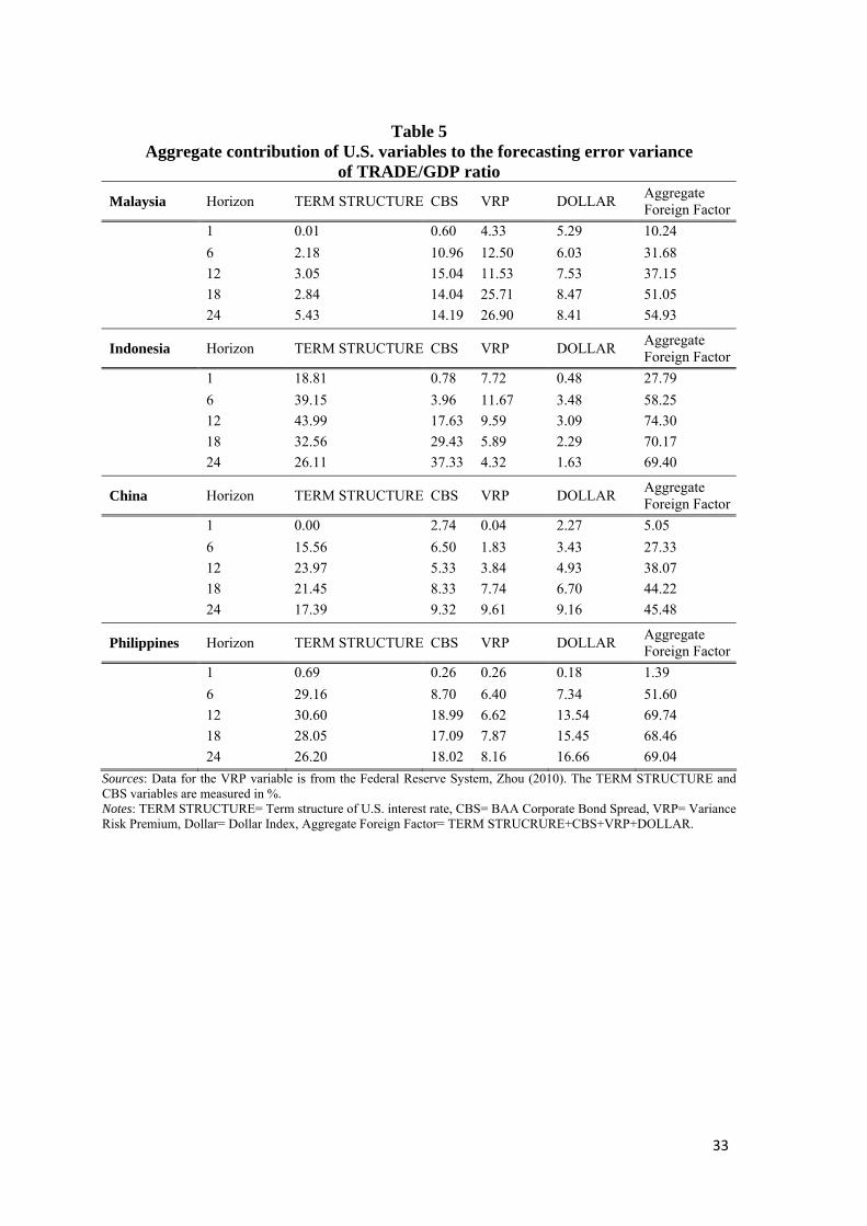
Table 5

Aggregate contribution of U.S. variables to the forecasting error variance of TRADE/GDP ratio

Malaysia Horizon TERM STRUCTURE CBS VRP DOLLAR Aggregate Foreign Factor

1 0.01 0.60 4.33 5.29 10.24 6 2.18 10.96 12.50 6.03 31.68 12 3.05 15.04 11.53 7.53 37.15 18 2.84 14.04 25.71 8.47 51.05 24 5.43 14.19 26.90 8.41 54.93

Indonesia Horizon TERM STRUCTURE CBS VRP DOLLAR Aggregate Foreign Factor

1 18.81 0.78 7.72 0.48 27.79 6 39.15 3.96 11.67 3.48 58.25 12 43.99 17.63 9.59 3.09 74.30 18 32.56 29.43 5.89 2.29 70.17 24 26.11 37.33 4.32 1.63 69.40

China Horizon TERM STRUCTURE CBS VRP DOLLAR Aggregate Foreign Factor

1 0.00 2.74 0.04 2.27 5.05 6 15.56 6.50 1.83 3.43 27.33 12 23.97 5.33 3.84 4.93 38.07 18 21.45 8.33 7.74 6.70 44.22 24 17.39 9.32 9.61 9.16 45.48

Philippines Horizon TERM STRUCTURE CBS VRP DOLLAR Aggregate Foreign Factor

1 0.69 0.26 0.26 0.18 1.39 6 29.16 8.70 6.40 7.34 51.60 12 30.60 18.99 6.62 13.54 69.74 18 28.05 17.09 7.87 15.45 68.46 24 26.20 18.02 8.16 16.66 69.04

Sources: Data for the VRP variable is from the Federal Reserve System, Zhou (2010). The TERM STRUCTURE and CBS variables are measured in %. Notes: TERM STRUCTURE= Term structure of U.S. interest rate, CBS= BAA Corporate Bond Spread, VRP= Variance Risk Premium, Dollar= Dollar Index, Aggregate Foreign Factor= TERM STRUCRURE+CBS+VRP+DOLLAR.

33

Table 6 Contribution of U.S. variables to the forecasting error variance of DEBT/GDP ratio

Malaysia Horizon TERM STRUCTURE CBS VRP DOLLAR Aggregate Foreign Factor

1 15.12 0.24 0.26 8.33 23.96 6 13.29 7.45 11.23 14.06 46.03 12 11.83 9.76 10.87 14.20 46.66 18 12.79 10.96 14.82 11.47 50.04 24 16.22 10.11 19.21 9.61 55.14

Indonesia Horizon TERM STRUCTURE CBS VRP DOLLAR Aggregate Foreign Factor

1 32.85 13.32 23.52 1.09 70.78 6 31.06 15.97 19.56 5.54 72.13 12 31.13 12.47 16.02 8.30 67.92 18 29.26 15.36 14.76 8.97 68.36 24 27.44 14.62 14.57 8.94 65.57

China Horizon TERM STRUCTURE CBS VRP DOLLAR Aggregate Foreign Factor

1 0.19 1.29 1.22 0.10 2.80 6 0.32 3.86 3.08 6.57 13.84 12 4.82 17.14 4.86 6.33 33.15 18 4.97 17.10 15.84 7.40 45.31 24 12.37 17.72 15.80 8.08 53.96

Philippines Horizon TERM STRUCTURE CBS VRP DOLLAR Aggregate Foreign Factor

1 0.01 0.38 6.64 7.44 14.46 6 5.02 4.43 7.80 11.82 29.06 12 8.73 12.17 7.33 10.60 38.83 18 8.69 12.74 7.13 11.29 39.85 24 18.56 16.77 8.13 10.35 53.81

Sources: Data for the VRP variable is from the Federal Reserve System, Zhou (2010). The TERM STRUCTURE and CBS variables are measured in %. Notes: TERM STRUCTURE= Term structure of U.S. interest rate, CBS= BAA Corporate Bond Spread, VRP= Variance Risk Premium, Dollar= Dollar Index, Aggregate Foreign Factor= TERM STRUCRURE+CBS+VRP+DOLLAR.

34

35

Table 7 Contribution of sovereign spread to the forecasting error variance

of domestic variables Malaysia Horizon TRADE/GDP DEBT/GDP

1 0.00 0.00 6 4.52 4.90 12 8.03 10.20 18 8.37 12.66 24 8.32 12.62 Indonesia Horizon TRADE/GDP DEBT/GDP

1 0.00 0.00 6 3.89 5.27 12 5.53 10.81 18 16.45 10.32 24 20.84 11.51 China Horizon TRADE/GDP DEBT/GDP

1 0.00 0.00 6 11.88 14.16 12 13.23 7.86 18 11.58 12.87 24 12.45 11.98 Philippines Horizon TRADE/GDP DEBT/GDP

1 0.00 0.00 6 3.47 6.97 12 3.12 9.65 18 5.42 10.38 24 6.51 9.02

Sources: All date are from DataStream. Notes: TRADE/GDP= Trade balance to GDP ratio and DEBT/GDP= Debt to GDP ratio.

Figure 1 Impulse response of sovereign spread to U.S. variable shocks

-.3

-.2

-.1

.0

.1

.2

.3

2 4 6 8 10 12 14 16 18 20 22 24

Response of LOGSPREAD to TERM STRUCTURE

-.3

-.2

-.1

.0

.1

.2

.3

2 4 6 8 10 12 14 16 18 20 22 24

Response of LOGSPREAD to CBS

-.3

-.2

-.1

.0

.1

.2

.3

2 4 6 8 10 12 14 16 18 20 22 24

Response of LOGSPREAD to VRP

-.3

-.2

-.1

.0

.1

.2

.3

2 4 6 8 10 12 14 16 18 20 22 24

Response of LOGSPREAD to DOLLAR

Malay sia

-.5

-.4

-.3

-.2

-.1

.0

.1

.2

.3

2 4 6 8 10 12 14 16 18 20 22 24


-.5

-.4

-.3

-.2

-.1

.0

.1

.2

.3

2 4 6 8 10 12 14 16 18 20 22 24


-.5

-.4

-.3

-.2

-.1

.0

.1

.2

.3

2 4 6 8 10 12 14 16 18 20 22 24


-.5

-.4

-.3

-.2

-.1

.0

.1

.2

.3

2 4 6 8 10 12 14 16 18 20 22 24


Indonesia

36

-.2

-.1

.0

.1

.2

2 4 6 8 10 12 14 16 18 20 22 24


-.2

-.1

.0

.1

.2

2 4 6 8 10 12 14 16 18 20 22 24


-.2

-.1

.0

.1

.2

2 4 6 8 10 12 14 16 18 20 22 24


-.2

-.1

.0

.1

.2

2 4 6 8 10 12 14 16 18 20 22 24


China

-.3

-.2

-.1

.0

.1

.2

2 4 6 8 10 12 14 16 18 20 22 24


-.3

-.2

-.1

.0

.1

.2

2 4 6 8 10 12 14 16 18 20 22 24


-.3

-.2

-.1

.0

.1

.2

2 4 6 8 10 12 14 16 18 20 22 24


-.3

-.2

-.1

.0

.1

.2

2 4 6 8 10 12 14 16 18 20 22 24


Philippines

Notes: solid lines depict point estimates of impulse response, and dotted lines depict 95% confident interval.

37

working paper no. 12-11 g the sovereign spread in asian

Documents