working paper 367 may 2014 - center for global … · working paper 367 may 2014 understanding...
TRANSCRIPT

Working Paper 367May 2014
Understanding Latin America’s Financial
Inclusion Gap
Abstract
This paper analyzes Latin America’s Financial Inclusion Gap, the difference between the average financial inclusion for Latin America and the corresponding average for a set of comparator countries. At the country level, we assess four types of obstacles to financial inclusion: macroeconomic weaknesses, income inequality, institutional deficiencies and financial sector inefficiencies. A key finding of this paper is that although the four types of obstacles explain the absolute level of financial inclusion, institutional deficiencies and income inequality are the most important obstacles behind the Latin America’s financial inclusion gap. From our analysis at the individual level, we find that there is a Latin America-specific effect of education and income. The results suggest that the effect of attaining secondary education on the probability of being financially included is significantly higher in Latin America than in its comparators. Furthermore, the difference in the probability of being financially included between the richest and the poorest individuals is significantly higher in Latin America than in comparator countries.
JEL Codes: D14, G21, G28
Keywords: Financial Inclusion, Latin America, Government Policy and regulation, Findex microdata
www.cgdev.org
Liliana Rojas-Suarez and Maria Alejandra Amado

Understanding Latin America’s Financial Inclusion Gap
Liliana Rojas-SuarezCenter for Global Development
Maria Alejandra Amado
Center for Global Development
The authors are especially grateful to Nancy Birdsall, Augusto de la Torre, Alan Gelb, Christian Meyer, Daniel Ortega, Lucciano Villacorta and participants in a session at the 2013 LACEA meetings in Mexico DF for their valuable comments and suggestions and Anita Tung for her contributions to this paper. A version of this paper was prepared for the CGD/CIEPLAN project: “Emerging Issues for Latin America and the Caribbean 2015-2020” sponsored by the Inter-American Development Bank (IADB). The authors alone are responsible for its content.
CGD is grateful for contributions from the Bill & Melinda Gates Foundation in support of this work.
Liliana Rojas-Suarez and Maria Alejandra Amado . 2014. “Understanding Latin America’s Financial Inclusion Gap” CGD Working Paper 367. Washington, DC: Center for Global Development. http://www.cgdev.org/publication/understanding-latin-america%E2%80%99s-financial-inclusion-gap-working-paper-367
Center for Global Development2055 L Street, NW
Fifth FloorWashington, DC 20036
202.416.4000(f ) 202.416.4050
www.cgdev.org
The Center for Global Development is an independent, nonprofit policy research organization dedicated to reducing global poverty and inequality and to making globalization work for the poor. Use and dissemination of this Working Paper is encouraged; however, reproduced copies may not be used for commercial purposes. Further usage is permitted under the terms of the Creative Commons License.
The views expressed in CGD Working Papers are those of the authors and should not be attributed to the board of directors or funders of the Center for Global Development.

Contents 1. Introduction ............................................................................................................................. 1
2. Financial Inclusion in Latin America: How does it compare with other country groups? ............................................................................................................................................... 3
3. Obstacles to Financial Inclusion in Latin America: Cross-Country Comparisons ....... 8
a. Socio-Economic Factors ................................................................................................... 8
b. Macroeconomic Constraints to Financial Inclusion ................................................... 11
c. Institutional Factors ......................................................................................................... 13
d. Financial Sector Inefficiencies and Inadequacies ........................................................ 15
4. Explaining Low Financial Inclusion in Latin America: An Econometric Analysis ... 18
a. Understanding Latin America’s Financial Inclusion Gap: a country-level analysis 19
b. Further Insights into the Latin America Financial Inclusion Gap: an individual-level analysis ................................................................................................................................ 28
5. Conclusions ............................................................................................................................ 35
Annex I: Grouping of countries by category ............................................................................ 40
Annex II: Correlation matrix of country-level variables .......................................................... 41
Annex III: Additional Variables included in the preliminary estimations ............................. 42
Annex IV: Validity of Instruments in the Endogeneity Analysis ........................................... 43
Annex V: Results under an Alternative Definition of the Financial Inclusion Gap ........... 45

1
1. Introduction
Financial inclusion, broadly defined as the share of households and firms that use formal
financial services, is increasingly recognized as crucial for development. Financial inclusion
can have substantial effects on welfare and can contribute to the reduction of poverty1. In
particular, financial inclusion allows individuals and firms to reduce the costs of making
transactions and to move away from short-term decision making toward an inter-temporal
allocation of resources. This encourages savings and improves incentives for productive
investments. As argued by Allen et al (2012), there is significant evidence supporting the
positive effects of having a bank account on individuals’ saving and investment behavior.
Although its importance is widely recognized -with a substantial amount of supporting
literature2-, financial inclusion remains extremely low in a large number of Latin American
countries. According to World Bank calculations for 20113, the percentage of adults that
have an account at a formal financial institution was only 30 percent in Colombia, 42 percent
in Chile and a dismal 14 percent in El Salvador and Nicaragua. Even in Brazil, the country
with the highest ratio of financial inclusion in the region, the ratio only reached 56 percent.
For the region as a whole, the average was 30 percent, far below the average ratio in high
income countries (89 percent) and even below the world average (46 percent). Most
importantly Latin America lagged significantly relative to countries with similar real income
per capita (henceforth, the region’s comparators). Specifically, financial inclusion in Latin
America’s comparators reached an average of 49 percent; that is, on average, financial
inclusion in the comparators group was over 60 percent higher than in Latin America. This
gap was similar when comparing median values. The median value of financial inclusion in
Latin America was 27.7 percent while that of its comparators equaled 45.5 percent.
This paper builds on existing research and new databases to address a fundamental question:
What are the relevant factors explaining the lower ratios of financial inclusion in Latin
America relative to comparable countries in terms of income per capita? In other words,
what explains the Latin American financial inclusion gap? At the country level, what is the role of
1See Beck, Demirgüç-Kunt, and Levine (2007) for an analysis of the effects of financial development on
poverty rates. For the linkages between access to formal financial services and poverty see Dupas and Robinson (2009) and Brune et al. (2011).
2 See for example Beck, Demirgüç-Kunt, and Honohan (2008) for an analysis of the theoretical models that illustrate the role access to finance plays in the development process. And Levine (2005) and Beck (2009) for an overview over the extensive literature on the relationship between finance and growth.
3 Global Findex Database, 2011. Available at http://www.worldbank.org/globalfindex.
2
macroeconomic vulnerabilities, socioeconomic constraints, institutional deficiencies and
financial sector inefficiencies? At the individual level, do demographic characteristics such as
sex, education or income affect financial inclusion in Latin America differently than in
comparator countries?
The inclusion of a variety of country variables for understanding the Latin American
financial inclusion gap builds up on the work of Rojas-Suarez (2007), among others, and is
based on the premise that financial intermediaries’ decisions are significantly influenced by
the economic and institutional environment where the financial system operates. For
example, it is expected that countries with greater institutional weaknesses are those where
challenges to improve financial inclusion could become more daunting. Financial institutions
might not be willing to extend the provision of financial services to large segments of the
population in societies where the respect for the rule of law, including enforcement of
contracts, is highly deficient. As shown below, relative to their comparators, most Latin
American countries are not favorably placed regarding the quality of their institutions. This
could, therefore, be a contributing factor explaining the region’s financial inclusion gap.
Another example of country-specific variables that are potential candidates to understand
the Latin American financial inclusion gap relates to the efficiency of the overall financial
system. It is expected that in financial systems with large operational inefficiencies reflected,
inter alia, in high administrative costs and/or a high degree of bank concentration, financial
services might only be offered at very high costs--above those in a competitive system--
which reduces usage of these services.4 On average, banks’ administrative costs are higher in
Latin America than in its comparators. This paper will explore whether this difference serves
to explain the financial inclusion gap.
Additional country-specific variables that could potentially explain the lower usage of
financial services in Latin America relative to its comparators include macroeconomic
fragilities, such as the region’s high volatility of inflation, and socioeconomic variables, such
as Latin America’s high income inequality—the highest among regions of the world.
The rest of the paper is organized as follows: Section 2 presents some stylized facts that
characterize financial inclusion in Latin America, highlighting differences with other country
groups, especially a set of countries categorized as the region’s comparators. Section 3
4 It’s been documented that high costs of maintaining deposit accounts and various types of fees on
financial services are important constraints to financial inclusion (see Allen et al and Beck et al).

3
identifies and discusses key obstacles at the country level affecting financial inclusion.
Section 4 presents an econometric analysis aimed at answering two questions: (a) At the
country level, which obstacles explain the lower levels of financial inclusion in Latin America
relatively to comparators? and (b) at the individual level, does belonging to Latin America
significantly affect individuals’ probability of being financially included, controlling for
demographic characteristics such as age, sex, education and income? Is there any Latin
American-specific effect of these individual characteristics? Section 5 concludes.
2. Financial Inclusion in Latin America: How does it compare with other country groups?
Until very recently, limited availability of data imposed a serious constraint on the empirical
analysis of financial inclusion.5 Over the past couple of years, however, important efforts
have emerged to overcome this problem.
At the regional level, the Andean Development Corporation (CAF, 2010) surveyed
households in 17 large Latin American cities to gauge information on key characteristics of
financial inclusion affecting the adult population, including factors deterring the demand for
financial services.6 Selected questions on financial inclusion were also included in the CAF’s
2011 survey, with plans to repeat the surveys in the years to come.7
At the global level, a World Bank project, named the Global Findex database was designed
to allow comparisons across country characteristics, individual characteristics, and over
time.8 The first round of the Findex database, covering the adult population (defined as 15
years of age and older) of 148 countries, was made public in 2011. While it is still too early to
count with time series data (updates are scheduled for 2014 and 2017), the common
methodology used in the country surveys allows sound cross-country and cross-individuals
comparisons.
5 Indeed, most cross-country analyses were based on an indicator of financial inclusion constructed by
Honohan (2007), based on multiple sources. See, for example, Rojas-Suarez (2010). 6 See CAF (2011) 7 Data from the surveys can be found in http://www.caf.com/view/index.asp?pageMs=74589&ms=19 8For complete information on the Global Findex project, see:
http://econ.worldbank.org/WBSITE/EXTERNAL/EXTDEC/EXTRESEARCH/EXTPROGRAMS/EXTFINRES/EXTGLOBALFIN/0,,contentMDK:23147627~pagePK:64168176~piPK:64168140~theSitePK:8519639,00.html

4
Table 1 to 3 present two indicators of financial inclusion taken from the Global Findex
database: the percentage of adults that have an account at a formal financial institution, and
the percentage of adults that have deposited savings at a financial institution in the past year.
The former indicator provides a stock measurement while the latter is a flow measurement
that is indicative of current activity by individuals in the usage of at least one category of
financial services: savings. The indicators are presented for Latin American countries and for
country groupings by income levels according to the World Bank categories.
Table 1 shows that, although with significant dispersion, no country in Latin America
financially includes the large majority of its population. In the countries with the highest
ratios, Brazil and Costa Rica, only half of the adult population has financial accounts.
Moreover, this ratio is extremely low (less than 25 percent) in Central American economies
(excluding Costa Rica), Paraguay, Peru and Uruguay. For this latter set of countries, the ratio
of inclusion to formal financial services is similar to that of the average for Sub-Saharan
Africa (24.1 percent)9, 10. An additional important result is derived from column 2: Although
a country comparison shows that the intensity of usage of savings accounts (column 2)
roughly corresponds to the penetration of financial inclusion (column 1)11, there are some clear
exceptions. In Argentina, only 3.8 percent of the adult population has saved in a formal
institution in 2010-11, the lowest number among the countries in our sample and out of line
with the penetration indicator of column 1 (33 percent). This is indicative of a potential
disintermediation process in Argentina; not a surprising result in the context of the ongoing
economic and financial difficulties faced by this country. As discussed below, by affecting
the demand for financial services, economic conditions play an important role as determinants
of financial inclusion12.
9 See World Bank (2012) 10 Of course it is possible that important segments of the population have access to financial services
provided in the informal sector. However, as mentioned in the introduction, this paper takes the view that there are important benefits in the provision of financial services through formal channels.
11 For example, Costa Rica, the country with the largest percentage of adult populations that have a financial account, is also the country with the largest percentage of adult populations that increased its savings in 2010-2011. Likewise, Nicaragua, displays one of the lowest ratio of financial inclusion in the region (14.2 percent) and a dismal percentage of the adult population that saved in 2010-11 (6.5 percent).
12 It is important to note that the indicators used in this paper do not reveal the existing huge differences in financial inclusion between urban and rural populations. By and large, the percentage of urban populations being financially included is much larger than the corresponding percentage in rural areas (a comprehensive analysis on financial inclusion in major urban areas in Latin America is included in CAF (2011)). Explaining the differential behavior in the usage of financial services between urban and rural areas is beyond the scope of this paper.

5
Table 1: Financial Inclusion Indicators in Latin America
Has an account at a formal financial
institution (1)
Has saved at a financial institution in the past year (1)
Argentina 33.1 3.8
Bolivia 28.0 17.1
Brazil 55.9 10.3
Chile 42.2 12.4
Colombia 30.4 9.2
Costa Rica 50.4 19.9
Dominican Republic 38.2 16.0
Ecuador 36.7 14.5
El Salvador 13.8 12.9
Guatemala 22.3 10.2
Honduras 20.5 8.5
Mexico 27.4 6.7
Nicaragua 14.2 6.5
Panama 24.9 12.5
Paraguay 21.7 9.7
Peru 20.5 8.6
Uruguay 23.5 5.7
Venezuela, RB 44.1 13.6
Latin America mean (unweighted) 30.4 11.0
Notes: (1) Percentage of adult population, 2011 Source: Authors’ calculations based on Global Financial Inclusion (Global Findex) Database, 2011
Table 2 divides the world into four groups of countries: High Income countries, Latin
American countries, Latin American comparators, and the rest of the world13. Latin
American comparators are defined as countries within the same range of real income per
capita as Latin American countries14. Annex I presents the list of countries within each
category.
13 High Income Countries are defined as those countries with values of income per-capita higher than those
of Latin America and its comparators. 14 This range goes from 879.9 to 9933.2 in constant 2000 US$ in 2009.

6
Latin America lags significantly relative to High Income countries in terms of the percentage
of the adult population with an account in a formal institution; the Latin American figure is
about one third of the corresponding number for high income economies. Moreover, Latin
America lags significantly with respect to its comparators, and is only moderately higher than
the rest of non-Latin American developing countries. This raises the issue about the
particular features of Latin America that may explain the low levels of financial inclusion.15
These issues will be dealt with in section 4.
The story for the flow indicator of financial inclusion (percentage of adult population who
saved in the period 2010-11) is similar to, but much more dramatic than that of the stock
variable. The percentage of the population who saved in Latin America is about one quarter
of the corresponding percentage in high income countries.
Table 2: Indicators of Financial Inclusion: Latin America and Other country Groups, 2011
Has an account at a formal financial
institution (1)
Has saved at a financial
institution in the past year (1)
Average Median Average Median
High Income Countries 89.3 94.6 45.3 49.5
Latin America 30.4 27.7 11.0 10.3
Latin American comparators 48.6 45.5 14.4 12.2
Rest of the World 18.3 17.3 8.8 7.7
Notes: (1) Percentage of adult population, 2011
Source: Global Financial Inclusion (Global Findex) Database, 2011
An additional indicator that is often used to complement the financial inclusion indicator is
banking system penetration through channels like bank branches and ATMs.16 These
indicators are taken from the Financial Access Survey (FAS), a database constructed by the
15 Which are actually closer to many of the poorest countries in the world than to the region’s comparators. 16 Ideally, the activities of the entire formal financial system would be accounted for rather than just the
banking system. However, no such data exists for world-wide comparisons, thus this indicator provides useful, albeit limited additional information.
7
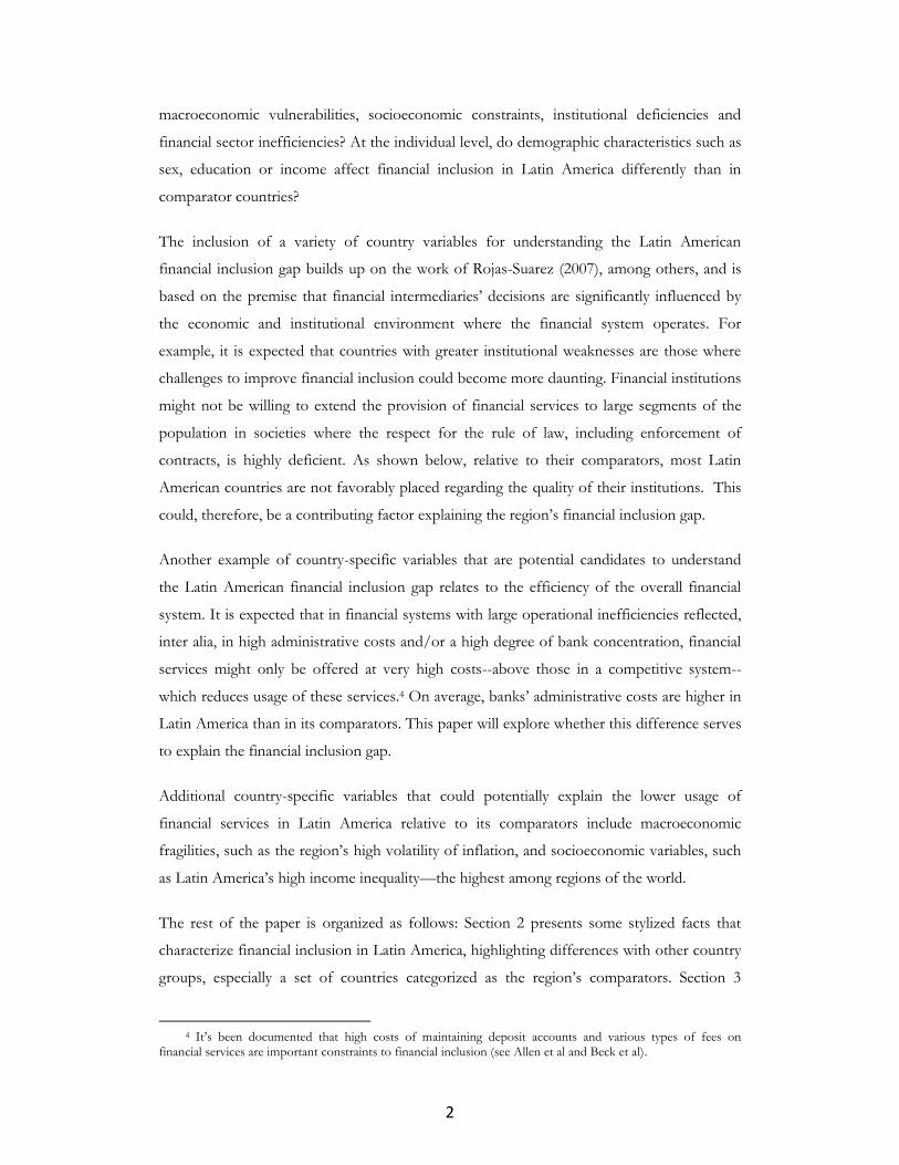
International Monetary Fund (IMF) 17and are presented in Table 3. The indicators consider
the number of bank branches and ATMs per 100,000 adults.
Table 3: Financial Inclusion through branches and ATMs (per 100,000 adult population, 2011)
Number of
Branches
Number of
ATMs
Number of ATMs
+ Branches
Unweighted Average
High Income Countries 34.3 99.4 134.2
Latin America 21.4 39.9 61.4
Latin American Comparators 19.3 43.6 63.3
Rest of the World 5.7 6.5 12.4
Source: IMF, Financial Inclusion Survey
The figures in Table 3 show a significant difference between high income countries and
Latin American countries in terms of bank coverage through branches and ATMs. However,
this gap is lower than that for the indicators of financial inclusion shown in Tables 1 and 2.
For example the average number of branches per 100,000 adults in Latin America is 63
percent of the corresponding value in high income countries and above the value of the
Latin American comparators.
However, an important caveat in assessing the importance of banks’ financial penetration
through branches and ATMS is that banks in a number of countries are using other channels
for the delivery of financial services, mostly based on digital technology. For example, for
Brazilian financial institutions, the most important form of reaching rural areas is through
non-bank correspondents; these are non-banking entities which provide banking services
through digital connections with a bank. This model has become increasingly popular and
has started to be applied in other Latin American countries such as Colombia, Mexico and
Peru. Similarly, in other countries like Bolivia, the large expansion of microfinance activities
is not necessarily based on the usage of branches or ATMs.
17 See www.fas.imf.org.

8
3. Obstacles to Financial Inclusion in Latin America: Cross-Country Comparisons
At the country level, the vast literature18 on financial inclusion has identified a number of
constraints for financial inclusion, both on the supply and the demand sides. In this section,
we follow the classification of factors affecting financial inclusion suggested by Rojas-Suarez
(2007) and further explored by Rojas-Suarez and Gonzales (2010) and discuss simple
correlations between financial inclusion and some of the most important identified
constraints. Here and in Section 4, the variable of financial inclusion used is the percentage
of the population that has at least one account at a formal financial institution. As explained
above, this indicator is taken from the Global Findex Database for the year 2011.
Obstacles affecting financial inclusion can be classified into four categories. The first
category relates to socio-economic constraints that limit both the supply of and the demand
for financial services. The second deals with vulnerabilities in the macroeconomic
environment that deters large segments of the population from using the services provided
by the formal financial system. The third category focuses on institutional weaknesses, with
emphasis on the quality of the governability of countries. Finally, the fourth category
identifies characteristics in the operations of the formal financial system that impede the
adequate provision of financial services. These operations respond both to the regulatory
framework and to the specific features of the financial system (such as the competitive
environment, business models, etc.). The discussion in this section provides insights on the
behavior of these obstacles for the Latin American region relative to its comparators. An
econometric investigation of these relationships will be undertaken in section 4.
a. Socio-Economic Factors
A number of papers19 have discussed the importance of socio-economic development in
explaining the degree of financial inclusion. Low levels of social indicators are often
associated with lower demand for and supply of financial services. As stated by Claessens
(2005), financial exclusion often reflects a wider social exclusion, which involves factors such
as education level, type of employment, and training.
Figure 1a shows this relationship by comparing the financial inclusion indicator and the UN
Human Development Indicator (HDI), which is a well-known measurement of social
18 As reviewed in Rojas-Suarez (2007) and Allen et al (2012). 19 Such as Claessens, 2005.

9
development. 20 The correlation coefficient between these two variables is 0.8. In general,
countries with greater access to social services and a better quality of life are countries that
have also developed a stronger “financial culture” in which the use of financial services
through formal markets becomes indispensable. In the graph, the countries denoted with
dark dots are those classified as high income economies. As expected, these countries display
the highest values of both the HDI and the indicator of inclusion.
Most Latin American countries are below the fitted line, suggesting that, ceteris paribus,
there is potential for improving financial inclusion given their degree of development. Thus,
other factors are constraining financial inclusion (explored in Section 4’s econometric
investigation). Uruguay, Mexico and Panama stand out. Their degree of financial inclusion is
well below what can be expected given their degree of social development. Such
homogeneous behavior cannot be found in Latin America’s comparator countries.
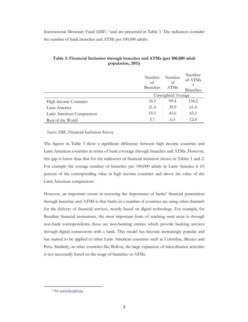
Alternatively, a country’s degree of social development could be proxied by the value of its
real GDP per capita. As shown in Figure 1b, the correlation between GDP per capita and
financial inclusion is highly positive (0.83) and of the same order of magnitude as the
correlation between social development and financial inclusion (0.83). As expected, the
20 The HDI has three components. The first relates to health, the second to education and the third to
income.
ARGBOL
BRA
CHL
COL
CRI
ECU
SLV
GTM HND
MEX
NIC
PANPRY PER
URY
Coef.correl=0.80p-value=0.000
02
04
06
08
01
00
Fin
an
cia
l In
clu
sio
n (
%)
.2 .4 .6 .8 1
Human Development Index (2011)
Comparators Rest of the World
Fitted values Latin America
High Income countries
Source: Authors' calculations based on United Nations Development Programe (2011) and Findex (2011)
Figure1a: Financial Inclusion and Social DevelopmentFigure 1a: Financial Inclusion and Social Development
10
behavior of Latin American countries is also similar to that in figure 1a and so is the
behavior of the comparators.21
Income distribution is another socio-economic factor potentially affecting financial
inclusion. Inequality can hinder financial reforms and financial development that enhance
financial inclusion. The argument is that in very unequal economies, with a highly skewed
distribution of income, wealth and political powers, powerful interests will likely block or
manipulate reforms so as to capture the benefits and avoid the costs (Claessens and Perotti,
2005). Behrman and Birdsall (2009) analyze the relationship between structural, high
inequality –measured by schooling inequality- and an index of financial liberalization for a
sample of 37 developing and developed countries. They conclude that in a highly unequal
setting, powerful interests are more likely to dominate politics, pushing for financial policies
that protect privileges rather than foster competition and growth.
Some authors, however, argue that there is some evidence suggesting that improved
household financial inclusion may lead to lower income inequality (see Honohan 2007).
Thus, there is the potential for reverse causality in the relationship between these two
variables.
21 This result is not surprising since GDP per capita is one of the components of the HDI and, as Pritchett
(2010) has noted the cross-country variability of the HDI is increasingly driven by GDP per capita.
ARGBOL
BRA
CHL
COL
CRI
ECU
SLV
GTMHND
MEX
NIC
PANPRY PER
URY
Coef. correl=0.83p-value=0.000
02
04
06
08
01
00
Fin
an
cia
l In
clu
sio
n (
%)
2 3 4 5
Log GDP per capita
Comparators Rest of the World
Fitted values Latin America
High Income countries
Source: Authors' calculations based on World Development Indicators (2012) and Findex (2011)
Figure1b: Financial Inclusion and GDP per capitaFigure 1b: Financial Inclusion and GDP per capita

11
While section 4 deals with the reverse causality issue, here we limit ourselves to the observed
correlation between financial inclusion and income inequality as measured by the Gini
coefficient (Figure 2). The correlation coefficient between the Gini and financial inclusion
equals -0.56 and is significant at the 1 percent level. Once again, high income countries
display greater financial inclusion and lower income inequality.
It is quite likely that the provision of financial services by financial institutions is relatively
easier in more egalitarian societies since financial products can be more uniform across a
large majority of the population. It is, therefore, not surprising that countries like Finland,
Denmark and Belgium, where almost 100 percent of their populations are financially
included, are also among the countries with the lowest values of the Gini coefficient. In
contrast, Latin American countries are largely concentrated in the lower right hand side of
the figure (the average and the median values of the Gini coefficient for Latin American
countries equal 51.4) While Gini coefficients in comparator countries are more dispersed,
the average (38.7) and the median (39.2) values are significantly lower than those for Latin
America.
b. Macroeconomic Constraints to Financial Inclusion
Macroeconomic instability can have adverse effects on financial inclusion. Significant
macroeconomic imbalances are associated with financial crises, sharply slowing the provision
ARGBOL
BRA
CHL
COL
CRI
ECU
SLV
GTM HND
MEX
NIC
PANPRYPER
URY
Coef. correl=-0.56p-value=0.000
02
04
06
08
01
00
Fin
an
cia
l In
clu
sio
n (
%)
20 30 40 50 60
Gini coefficientlatest observation since 2000
Comparators Rest of the World
Fitted values Latin America
High Income countries
Source: Authors' calculations based on World Income Inequality Database (WIID- v. 2.0a) and Findex (2011)
Figure 2: Financial Inclusion and Income InequalityFigure 2: Financial Inclusion and Income Inequality

12
of financial services. But beyond credit supply effects, the negative consequences on the
demand for financial services are usually quite severe and may last well after the end of a
financial crisis. The reason is that the demand for deposits and savings products offered by
the formal financial system depends largely on trust in the soundness of the system. The
economic and financial crises in emerging markets and developing countries in the last three
decades have resulted in significant losses for depositors in terms of the real value of their
wealth. Deposits’ freeze, interest rate ceilings, forced conversion of foreign-currency
denominated deposits into local currency-denominated deposits using undervalued exchange
rates, and hyperinflation that destroyed the value of savings in the financial system were
among the causes.22
High inflation volatility and real interest rates perhaps best capture the adverse effect of
macro instability on the demand for financial services. Figure 3 shows the negative
correlation between the coefficient of variation of inflation23 and the indicator of financial
inclusion. The inverse relationship between these variables is reflected in a correlation
coefficient of -0.30, significant at the 1 percent level. Most high income economies (denoted
with dark dots) are located at the upper left hand side of the graph. Clearly, high income
countries have the lowest inflation volatility and the highest values for financial inclusion,
suggesting a high willingness to demand (and supply) services offered by the formal financial
system. Among Latin American countries, Peru and Argentina have the greatest inflation
volatility, followed by Brazil. This high volatility in part reflects the extremely high inflation
rates in the early 1990s and the speculative balance of payments crises in the late 1990s in
Brazil and Peru. The highest ratio of financial inclusion displayed by Brazil (among Latin
American countries) cannot be explained by a long history of macroeconomic stability as the
country does not have one. Other country-specific policies and factors are behind Brazil’s
advances with financial inclusion. With escalating inflation in the last years, problems in
Argentina are as current today as they were in the 1990s. By contrast, Chile and Costa Rica
have the combination of low inflation volatility and relatively high (among countries in the
region) financial inclusion indicators. The average and median values of inflation volatility
for Latin America and its comparators countries do not diverge significantly (1.3 and 1.0
respectively in Latin America and 1.4 and 1.2 respectively in the comparator countries). The
22 Although the recent global financial crisis severely affected developed countries, especially the US, in
general, depositors did not suffer losses in the real value of their deposits. This is because a number of advanced economies have in place credible deposit insurance schemes—a result of these countries’ capacity to issue “hard currency”, that is currencies that are internationally traded and enjoy high liquidity worldwide.
23 Approximated by the ratio standard deviation to average inflation, calculated over the period 1990-2011.

13
values in both groups, however, differ significantly from those in high income countries (0.7
and 0.5 respectively)
c. Institutional Factors
The importance of institutional quality in the provision of financial services has been
discussed extensively in the literature.24 The institutional environment in which financial
entities operate plays a central role in the provision of financial services.
To measure institutional quality, this paper uses the Worldwide Governance Indicators.25
Previous studies26 have demonstrated that the financial system will develop more fully in
countries with observance of the law, political stability, fair and efficient enforcement of the
rule of law and respect for creditors’ and debtors’ rights. When contracts between creditors
and debtors are observed, depositors have incentives to entrust their savings to banks and
other financial institutions. Also, financial firms have incentives to lend at better rates and
longer terms to enterprises, since they can seize collaterals when default happens and are
compensated according to pre-established rules in bankruptcy. In a recent paper, Allan et al
(2012) show that two measures of creditors’ rights—the “legal right index” from the World
24 An analysis of the effect of institutional quality on access to bank services is found in Beck et al. (2003). 25 www.govindicators.org 26 See for example, Claessens and Leaven (2003) and Demetriades and Andrianova (2004).
ARGBOL
BRA
CHL
COL
CRI
ECU
SLV
GTMHND
MEX
NIC
PANPRY PER
URY
Coef. correl=-0.30p-value=0.000
02
04
06
08
01
00
Fin
an
cia
l In
clu
sio
n (
%)
0 1 2 3 4 5
InflationCoefficient of variation 1990-2011
Comparators Rest of the World
Fitted values Latin America
High Income countries
Source: Authors' calculations based on IMF World Economic Outlook (WEO) and Findex (2011)
Figure 3: Financial Inclusion and Inflation VolatilityFigure 3: Financial Inclusion and Inflation Volatility

14
Bank Doing Business and the “political risk rating” from the International Country Risk
Guide-- play an important role in the usage of bank accounts.
Figure 4 illustrates the relationship between institutional quality and financial inclusion using
the Rule of Law component of the Worldwide Governance Indicators, which measures
agents’ confidence in and commitment to abiding by the rules of society, the quality of
contract enforcement, the police, the courts and the likelihood of crime and violence. In this
graph we are using the variable Weak Law, which is a transformation of the rule of law
indicator and ranges from -100 to 0. The graph shows a clear negative (positive) relationship
between weak law (adherence to the rule of law) and financial inclusion. The correlation
coefficient is -0.83 and is significant at the 1 percent level.
As expected, high income economies are concentrated in the upper left corner of the graph,
indicating that high institutional quality in developed countries is consistent with high levels
of financial inclusion. Among Latin American countries, Chile is the closest to high income
economies in terms of quality of institutions.27 At the opposite extreme, a number of Central
American countries, including Nicaragua, El Salvador, Honduras and Guatemala, Bolivia,
and Paraguay display very low institutional quality and very low financial inclusion. Relative
to its comparators, Latin American countries do not stand favorably. On average, the weak
law indicator reaches a value of -40 in Latin America while the corresponding value in
27 However, despite its high level of institutional quality, Chile still lags in terms of financial inclusion,
relative to Brazil and Costa Rica.
ARGBOL
BRA
CHL
COL
CRI
ECU
SLV
GTMHNDMEX
NIC
PANPRYPER
URY
Coef. correl=-0.83p-value=0.000
-50
05
01
00
Fin
an
cia
l In
clu
sio
n (
%)
-100 -80 -60 -40 -20 0
Weak Law
Comparators Rest of the world
Fitted values Latin America
High Income countries
Source: Authors' calculations based on The Worldwide Governance Indicators (2010) and Findex (2011)
Figure 4: Financial Inclusion and Quality of InstitutionsFigure 4: Financial Inclusion and Quality of Institutions

15
comparator countries equals -46. This difference is significantly larger if we take median
values. Weak law in the median Latin America country is -35, while it is -44 in the median
comparator country.
d. Financial Sector Inefficiencies and Inadequacies
Based on Rojas-Suarez (2007), in this category we include obstacles to financial inclusion
encountered by individuals and firms that can be attributed to characteristics of the financial
system, including financial entities’ methods and practices in conducting their operations.
Operational inefficiencies reflected, for example, in high administrative costs and/or a high
degree of concentration can result in important constraints for financial inclusion.28 Financial
system’s inefficiencies tend to restrict the availability of financial products and to increase the
price of accessing them. High costs of opening and maintaining an account in a financial
institution (above the costs in more efficient systems) and high minimum balances
requirements are byproducts of these inefficiencies.29
The ratio of overhead (administrative) costs to total assets is commonly used as an indicator
of banks’ operational inefficiency. High ratios tend to increase the fixed costs of extending
loans and maintaining accounts as well as lowering interest payments on savings and other
deposits, therefore restricting financial inclusion.
Figure 5, presents the relationship between the ratio of bank overhead costs to total assets
and financial inclusion. The correlation coefficient equals -0.55 and is significant at the 1
percent level.
28 A number of financial system inefficiencies can in turn, be associated with inadequate policies and
regulations 29 Beck et al (2006) and Allen et al (2012) use survey data to the analyze costs of opening and maintaining
bank accounts. However, the data in Beck et al cover only 62 countries and that in Allen et al (2012) is not publicly available.

16
The figure shows results similar to those in previous graphs in the sense that high income
countries display the lowest ratios of operational inefficiency (lower overhead costs).30
Among Latin American countries, Paraguay stands out for having the highest ratios of bank
operational inefficiency and one of the lowest values of the indicator of financial inclusion in
the region. While Chile displays ratios similar to those in high income countries, the average
and the median Latin American country have ratios of operational inefficiency much higher
than the average comparator country. Indeed, the median value for Latin America (4.8
percent) is over 50 percent higher than the median value for comparator countries (2.7
percent).
Banking concentration can also be considered a measure of financial inefficiency to the
extent that it might lead to oligopolistic behavior. In addition to driving up the costs of
providing financial services, high levels of banking concentration might also inhibit lending
to individuals and SMEs if concentration is associated with a lack of competitive incentives
to assess the quality of borrowers with relative riskier characteristics. However, recent
studies have found that highly concentrated banking systems become an obstacle to financial
inclusion mostly in those countries with weak institutions and strong restrictions on the
range of permissible banking activities.31 At places where contract enforcement is weaker,
30 The data is the average for 2006-2010 to smooth out the effects of the global financial crisis. 31 See, for example, Claessens (2005).
ARGBOL
BRA
CHL
COL
CRI
ECU
SLV
GTM HNDMEX
NIC
PANPRYPER
URY
Coef. correl=-0.55p-value=0.000
-50
05
01
00
Fin
an
cia
l In
clu
sio
n (
%)
0 2 4 6 8 10
Overhead Costs (% of total assets)Average 2006-2010
Comparators Rest of the world
Fitted values Latin America
High Income countries
Source: Authors' calculations based on Fitch’s BankScope database (2010) and Findex (2011)
Figure 5: Financial Inclusion and Bank InneficiencyFigure 5: Financial Inclusion and Bank Inefficiency

17
the oligopolistic power arising from a high banking concentration leads to greater
discrimination against riskier borrowers (like low-income individuals and SMEs) and to
higher costs of opening and maintaining accounts than there would be in a more competitive
banking system.
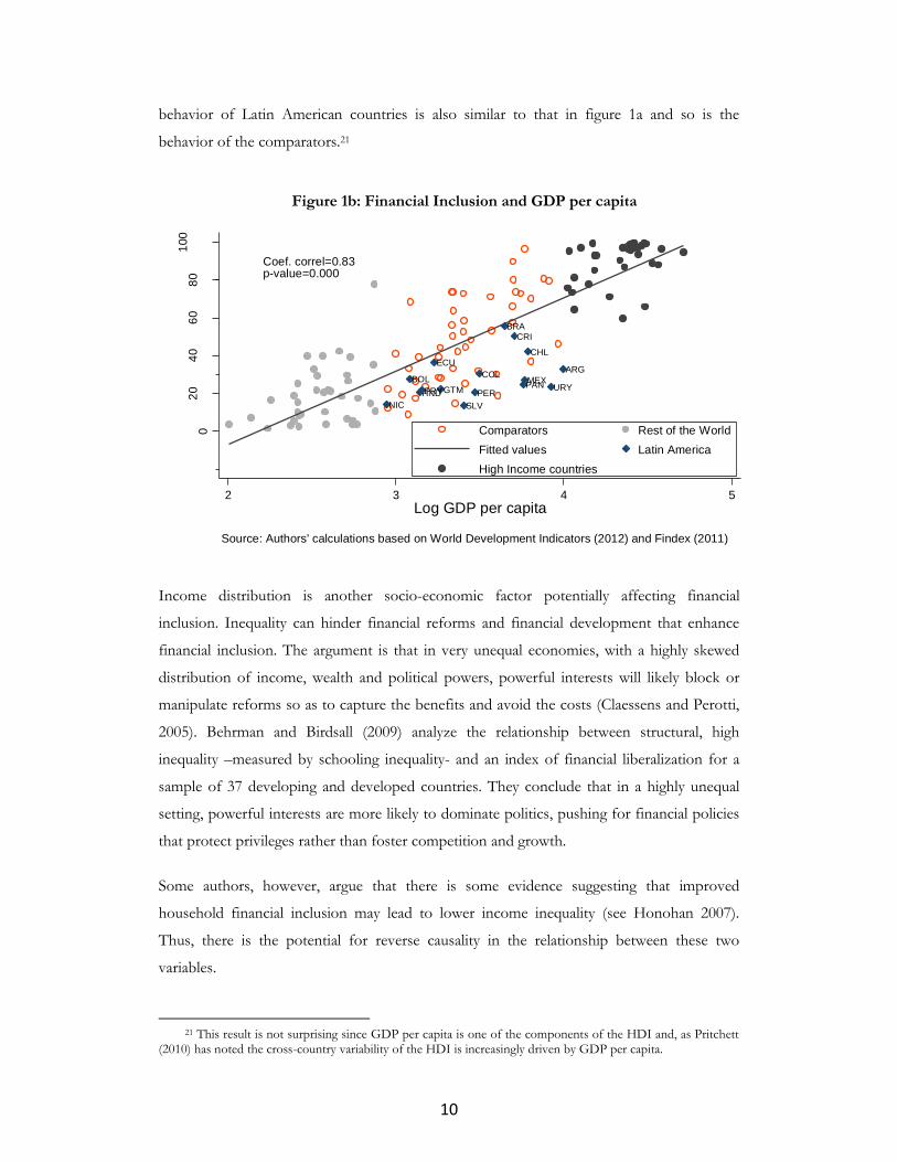
Taken together, figures 6a and 6b are consistent with these claims. In figure 6a the
correlation between bank concentration32 and financial inclusion is negative but only reaches
the value of -0.2.
Figure 6b plots financial inclusion and bank concentration for two groups of countries. For
illustrative purposes we have arbitrarily defined “low weak-law countries” as the ones whose
weak law levels are below the average of the sample, and “high-weak law countries” as the
ones whose weak law levels are above the average. As expected, almost all high income
countries fall into the first category. However, the correlation coefficient between bank
concentration and financial inclusion for the sample of “low weak-law countries” is not
significant and, therefore, we cannot determine statistically that there is a relationship
between those variables. In contrast, in the sample of “high weak-law countries” we find a
significant and negative correlation between bank concentration and institutional quality of -
0.3. In fact, most Latin American countries are within this group, suggesting that bank
32 Defined as the percentage of total system assets held by the three largest banks.
ARGBOL
BRA
CHL
COL
CRI
ECU
SLV
GTMHND
MEX
NIC
PANPRY PER
URY
Coef. correl=-0.2p-value=0.021
02
04
06
08
01
00
Fin
an
cia
l In
clu
sio
n (
%)
20 40 60 80 100
Bank concentration (%)
Comparators Rest of the world
Fitted values Latin America
High Income countries
Source: Authors' calculations based on Fitch’s BankScope database (2009) and Findex (2011)
Figure 6a: Financial Inclusion and Bank Concentration
Figure 6: Financial Inclusion and Bank Concentration
18
concentration could be an obstacle to financial inclusion in this region. Nevertheless, the
average and mean percentage values of bank concentration in Latin America (59.1 and 57.7
respectively) do no differ significantly from those of its comparators (58.5 and 58.7
respectively).
We therefore hypothesize that in countries with strong institutions, such as the high income
countries, the net adverse effect of high bank concentration on financial inclusion is much
lower (and perhaps even insignificant) than in countries with weak institutions. This issue
will be discussed further in the next section when we formally analyze the overall effects of
bank concentration.
4. Explaining Low Financial Inclusion in Latin America: An Econometric Analysis
This section conducts an econometric analysis to understand the relatively low degree of
financial inclusion in Latin America. First, based on country-level data, we estimate a
benchmark equation using a worldwide sample of 137 countries and analyze the Latin
American financial inclusion gap -relative to comparator countries-. For this purpose, we
BRA
CHL
CRI
URY
Coef. correl=-0.30p-value=0.0094
Coef. correl=0.12p-value=0.3266
ARGBOL
COL
ECU
SLV
GTMHND
MEX
NIC
PANPRY PER
05
01
00
20 40 60 80 100 20 40 60 80 100
Source: Authors' calculations based on Fitch’s BankScope database (2009) and Findex (2011)
Low weak-law countries High weak-law countries
Figure 6b: Financial Inclusion and Bank Concentration
Comparators Rest of the world
Fitted values Latin America
High Income countries
Fin
an
cia
l In
clu
sio
n (
%)
Bank Concentration (%)
Note: Low-weak law countries are countries whose weak law levels are below -47.64.
High-weak law countries are the remaining countries in the sample.
Figure 6b: Financial Inclusion and Bank Concentration

19
include the different obstacles discussed in the previous section as controls in the
benchmark equation. Second, using individual-level data, we evaluate whether belonging to a
Latin American country significantly affects individual’s probability of being financially
included; controlling for demographic characteristics such as age, sex, education and income.
Also, we evaluate whether there is any Latin American-specific effect of these individual
characteristics. While we acknowledge that there are additional individual characteristics that
might be relevant in explaining financial inclusion, our analysis is limited to these four
characteristics because of data availability.
a. Understanding Latin America’s Financial Inclusion Gap: a country-
level analysis
a.1. The model and data
As discussed above, the obstacles affecting financial inclusion at the country-level are taken
from the theoretical and empirical literature and can be classified into four categories
(following Rojas-Suarez, 2007). Based on that literature, we follow a similar methodology as
in Rojas-Suarez and Gonzales (2010) and estimate the following equation:
0 1
(1) _ _ _n
i i i k ki ikFin Inclusion Latin America Outside comp Y
Where i denotes a country, _Fin Inclusion is the percentage of the adult population that
holds an account at a formal financial institution, kY is a vector representing the different
obstacles to financial inclusion. _Latin America is a dummy indicating a Latin American
country, _Outside comp is a dummy indicating a country outside Latin American comparators
(that is, countries that are neither Latin American countries nor their comparators); and is
assumed to be a disturbance with the usual properties of zero mean and constant variance.
The Latin America dummy is taken here to reflect the region’s financial inclusion gap relative
to comparators. As discussed above, comparator countries are defined as those with a similar
real income per capita as Latin America (see Annex I).
Since there is no time series data available for the dependent variable, _Fin Inclusion , we
are restricted to using a cross-section data set in the estimation of equation (1). Data for the
dependent variable corresponds to 2011. For the explanatory variables, we use the latest
available data.

20
The discussion in Section 3 provided the basis for identifying the variables to conduct the
econometric exercise. However, the presence of multicollinearity prevented the simultaneous
inclusion of all controls discussed in section 3. For example, the degree of social
development and the quality of institutions (reflected by the variable Weak_Law) were highly
correlated (a correlation coefficient of 0.75). We also considered an additional set of
variables that could be classified within any of the four categories of obstacles. Annex III
presents the entire list of variables considered and their sources. In some cases, data
availability precluded the inclusion of some variables; in others multicollinearity was the
constraint.
The explanatory variables included in the regressions presented in Table 5 are:
Income_Inequality: is the latest observation of the Gini coefficient available since 2000.
This variable is taken from the World Income Inequality Database (WIID) and represents
the category of socioeconomic factors.
Inflation_Volatility: is the coefficient of variation of inflation, measured as the ratio of the
standard deviation of annual inflation (end of period) to average inflation, for the period
1990-2011. This variable was constructed using the IMF World Economic Outlook database
and represents the category macroeconomic constraints.
Weak_Law: this variable represents the lack of enforcement of the Rule of Law, an
indicator taken from the Worldwide Governance Indicators for the year 2010. The rule of
law “reflects perceptions of the extent to which agents have confidence in and abide by the
rules of society, and in particular the quality of contract enforcement, property rights, the
police, and the courts, as well as the likelihood of crime and violence.”33 The original
variable, rule of law, was rescaled to a range from 0 to 100, and the variable Weak_Law is
calculated by multiplying the rescaled variable by minus 1. This variable belongs to the
category institutional factors.
Overhead_Costs: An indicator of banking operational inefficiencies, measured as the ratio
of overhead costs to total assets. This variable was taken from the dataset created by Beck et
al., and updated in 2012. The original data is from the Fitch BankScope database. The
variable used in the regression is the average 2006-2010 and is within the category of financial
sector inefficiencies.
33 www.govindicators.org.

21
Bank_Concentration: measured as the share of the three largest banks’ assets to all
commercial banks’ assets. This variable was taken from the dataset created by Beck et al.,
and updated in 2012. The original data is from the Fitch BankScope database. The variable
used in the regression is from 2009 and is within the category of financial sector inefficiencies.
In addition to these obstacles to financial inclusion, we also considered real GDP per capita
as a control in the empirical analysis. This is consistent with the discussion in section 3. Real
GDP per capita is measured in logs and defined as follows:
Log_GDP_per_capita: corresponds to the logarithm of GDP per capita in constant 2000
US dollars of 2009. The variable is taken from the World Bank World Development
Indicators database.
The variables Log_GDP_per_capita and Weak_Law are highly correlated.34 Thus, to avoid
multicollinearity, the analysis that follows presents two sets of regressions. In the first one
we control for the effects of institutional quality and in the second one for the effect of real
income per capita.
a.2. Econometric strategy
As a first step we estimate a simple OLS regression including the dummy for Latin America
and a dummy for countries outside comparators (see table 5 column 1). The coefficient of
the Latin America dummy reflects the difference between the average financial inclusion in
Latin America and its comparators (18.1 percentage points in absolute terms). As mentioned
before, we call this difference: the Latin American financial inclusion gap. Our purpose is to
evaluate whether the incorporation of alternative obstacles to financial inclusion in the
regression can help to understand this gap.
Before proceeding, however, we need to deal with possible endogeneity issues. The strict
exogeneity of each obstacle included in the regression is a necessary condition to draw any
conclusion about their effects on the gap. As mentioned in section 3, the literature shows
evidence of a relationship between financial inclusion and one of the obstacles considered in
the regression, Income_Inequality, which might be driven by reverse causation. This generates a
potential problem of endogeneity of income inequality. We, therefore, test for potential
endogeneity and evaluate the convenience of using instrumental variables estimation (IV) to
deal with this problem.
34 Both variables present a correlation coefficient that exceeds the practical benchmark of 0.75.

22
We use the Durbin-Wu-Hausman test to test for endogeneity of Income_Inequality. Following
the insights in Calderon and Chong (2001) we use trade variables as instruments for
Income_Inequality. Specifically, we use an indicator of trade openness, Trade_Opennes, which is
the ratio of exports and imports to GDP in 201035 and the interaction term between trade
openness, and a concentration index of merchandise exports and imports of 201036,
Trade_Concentration37. The hypothesis is that although higher levels of trade openness
decrease income inequality, this effect is reduced at high levels of trade concentration.38
Annex IV verifies the validity of the selected instruments.
The p-values of the Durbin-Wu-Hausman test of endogeneity are shown in Table 4.
Table 4: Instrumented Variable: Income_Inequality
Excluded Instruments Durbin-Wu-
Hausman p-value
Trade_Openness Trade_Openness*Trade_Concentration
0.311764 0.5782
(*) H0: variables are exogenous
Results show that it is possible to reject the endogeneity of Income_Inequality in the regression,
suggesting that OLS is the best estimator, a consistent and more efficient estimator than the
Instrumental Variables (IV) estimator.
35 Data for constructing this indicator is obtained from the World Bank Database.
http://data.worldbank.org/ 36 This indicator is the Herfindahl-Hirschmann index, normalized to obtain values ranging from 0 to 1
(maximum concentration). Data is obtained from the United Nations Conference on Trade and Development (UNCTAD) database. http://unctad.org/en/pages/Statistics.aspx
37 We argue that these instruments are strictly exogenous –they are not correlated with any shock affecting financial inclusion-.
38 Calderon and Chong (2001) show that trade openness reduce income inequality, measured by the Gini coefficient. They also find that export orientation towards primary activities may be associated with higher income inequality. This last finding supports the hypothesis that higher trade concentration reduces the effect of trade openness on income inequality, since countries with higher levels of exports concentration are mainly commodities exporters.

23
a.3. Results
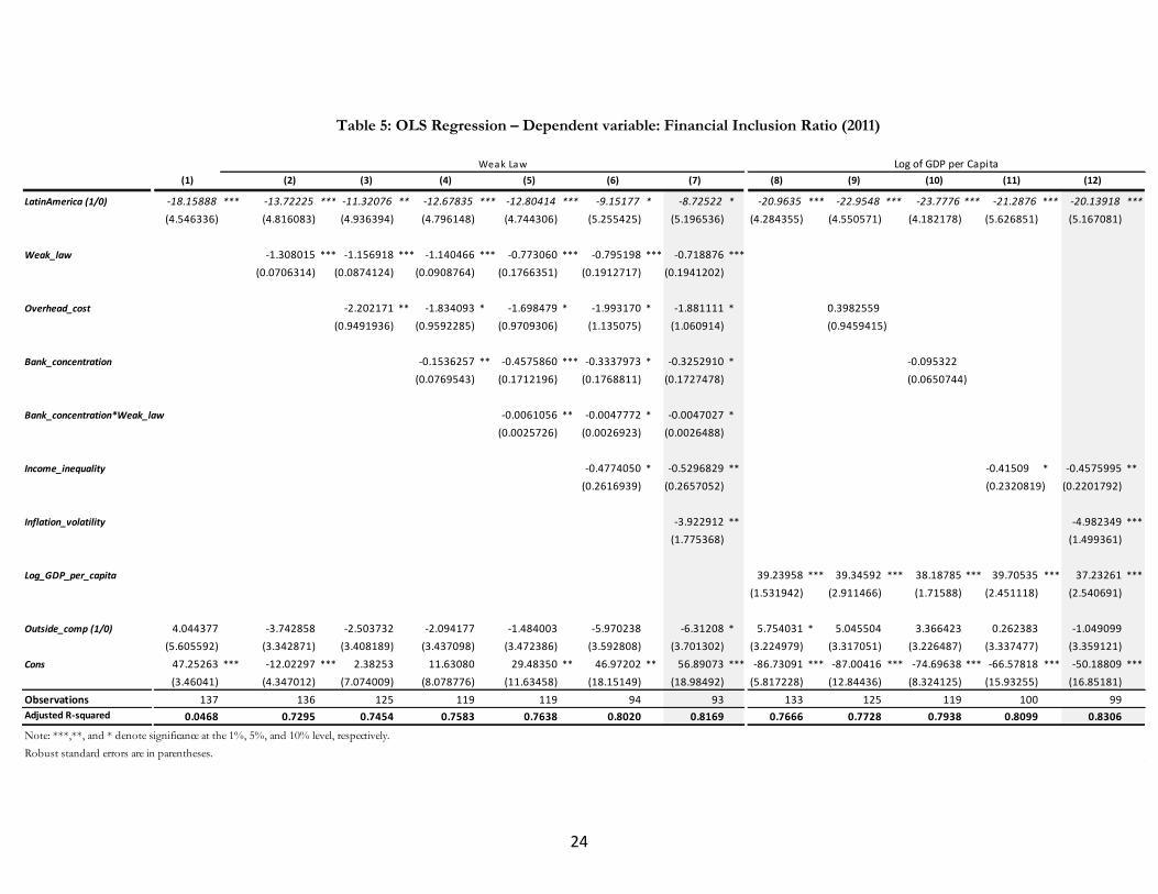
Based on OLS estimations, columns (2) to (7) of Table 5 include the variable Weak_Law as a
control, while columns (8) to (12) include the Log_GDP_per_capita. The shadowed columns
(7) and (12) indicate the preferred specifications under the two alternatives.
We focus first on the regressions including Weak_Law as a control. We expected a negative
sign for the coefficients of all the explanatory variables in these regressions since the
variables are expressed as obstacles to financial inclusion. There are two central results from
the preferred specification in column (7). The first is that all the variables considered are
significant and the goodness of fit reaches a high value (the adjusted R-squared equals 0.81).
The second is that, in comparison to column (1), the absolute value of the coefficient of the
Latin America dummy declines significantly to 8.7 (in absolute terms). This last result, in
turn, implies that the obstacles to financial inclusion in the regression can account for more
than half of the Latin American financial inclusion gap.
How do the alternative obstacles to financial inclusion help to understand the Latin American
financial inclusion gap? The entire set of regressions (columns (2) to (6)) serves to answer this
question since in each consecutive column we add an additional variable representing an
obstacle. The order of inclusion of obstacles does not affect the results in any meaningful
way.
The analysis shows that the quality of institutions, represented by the variable Weak_Law is
the relatively most important factor to understand the Latin American financial inclusion gap. As
shown in column (2), the addition of this variable reduces the coefficient of the Latin
America dummy by over 4 percentage points. Moreover, the goodness of fit of the simple
model in column (2) is quite high (the adjusted R-squared equals 0.72).
The variables Overhead_Costs and Inflation_Volatility (incorporated in the regression in
columns (3) and (7)) are significant as obstacles explaining the dependent variable, financial
inclusion, but play a relatively less important role for understanding the Latin American
financial inclusion gap; that is, the coefficient of the Latin America dummy only shows a slight
decrease in absolute terms when these variables are incorporated in the regression. In
addition, Bank_Concentration, while significant on its own or when interacted with Weak_Law
(columns 4 and 5 respectively) cannot explain the Latin American financial inclusion gap since
the coefficient of the Latin America dummy increases (in absolute terms) when these
variables are introduced.
24
Table 5: OLS Regression - Dependent variable: Financial Inclusion Ratio (2011)
(1) (2) (3) (4) (5) (6) (7) (8) (9) (10) (11) (12)
LatinAmerica (1/0) -18.15888 *** -13.72225 *** -11.32076 ** -12.67835 *** -12.80414 *** -9.15177 * -8.72522 * -20.9635 *** -22.9548 *** -23.7776 *** -21.2876 *** -20.13918 ***
(4.546336) (4.816083) (4.936394) (4.796148) (4.744306) (5.255425) (5.196536) (4.284355) (4.550571) (4.182178) (5.626851) (5.167081)
Weak_law -1.308015 *** -1.156918 *** -1.140466 *** -0.773060 *** -0.795198 *** -0.718876 ***
(0.0706314) (0.0874124) (0.0908764) (0.1766351) (0.1912717) (0.1941202)
Overhead_cost -2.202171 ** -1.834093 * -1.698479 * -1.993170 * -1.881111 * 0.3982559
(0.9491936) (0.9592285) (0.9709306) (1.135075) (1.060914) (0.9459415)
Bank_concentration -0.1536257 ** -0.4575860 *** -0.3337973 * -0.3252910 * -0.095322
(0.0769543) (0.1712196) (0.1768811) (0.1727478) (0.0650744)
Bank_concentration*Weak_law -0.0061056 ** -0.0047772 * -0.0047027 *
(0.0025726) (0.0026923) (0.0026488)
Income_inequality -0.4774050 * -0.5296829 ** -0.41509 * -0.4575995 **
(0.2616939) (0.2657052) (0.2320819) (0.2201792)
Inflation_volatility -3.922912 ** -4.982349 ***
(1.775368) (1.499361)
Log_GDP_per_capita 39.23958 *** 39.34592 *** 38.18785 *** 39.70535 *** 37.23261 ***
(1.531942) (2.911466) (1.71588) (2.451118) (2.540691)
Outside_comp (1/0) 4.044377 -3.742858 -2.503732 -2.094177 -1.484003 -5.970238 -6.31208 * 5.754031 * 5.045504 3.366423 0.262383 -1.049099
(5.605592) (3.342871) (3.408189) (3.437098) (3.472386) (3.592808) (3.701302) (3.224979) (3.317051) (3.226487) (3.337477) (3.359121)
Cons 47.25263 *** -12.02297 *** 2.38253 11.63080 29.48350 ** 46.97202 ** 56.89073 *** -86.73091 *** -87.00416 *** -74.69638 *** -66.57818 *** -50.18809 ***
(3.46041) (4.347012) (7.074009) (8.078776) (11.63458) (18.15149) (18.98492) (5.817228) (12.84436) (8.324125) (15.93255) (16.85181)
Observations 137 136 125 119 119 94 93 133 125 119 100 99
Adjusted R-squared 0.0468 0.7295 0.7454 0.7583 0.7638 0.8020 0.8169 0.7666 0.7728 0.7938 0.8099 0.8306
Note: ***,**, and * denote significance at the 1%, 5%, and 10% level, respectively.
Robust standard errors are in parentheses.
Weak Law Log of GDP per Capita
Table 5: OLS Regression – Dependent variable: Financial Inclusion Ratio (2011)
25
In contrast, controlling for Income_Inequality (column (6) reduces the absolute value of the
dummy coefficient from 12.8 to 9.1 and also has a significant effect in explaining financial
inclusion.
Taken together, these findings imply that, while all obstacles considered significantly explain
the behavior of financial inclusion in a world-wide cross-country analysis, institutional
deficiencies and income inequality are at the core of understanding the low levels of financial
inclusion in the Latin American region relative to the region’s comparators. To clarify:
Improvements in all and every one of the obstacles analyzed support an increase in the absolute
levels of financial inclusion for the countries in the sample: Latin America and otherwise.
However, to attain large reductions in the financial inclusion gap between Latin America as a
whole and its comparators, improvements in institutional quality and income inequality are
essential.
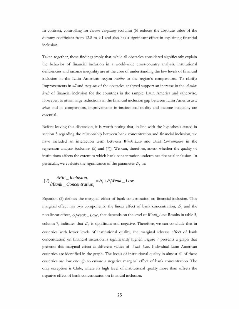
Before leaving this discussion, it is worth noting that, in line with the hypothesis stated in
section 3 regarding the relationship between bank concentration and financial inclusion, we
have included an interaction term between Weak_Law and Bank_Concentration in the
regression analysis (columns (5) and (7)). We can, therefore, assess whether the quality of
institutions affects the extent to which bank concentration undermines financial inclusion. In
particular, we evaluate the significance of the parameter 2 in:
1 2
_(2) _
_
ii
i
Fin InclusionWeak Law
Bank Concentration
Equation (2) defines the marginal effect of bank concentration on financial inclusion. This
marginal effect has two components: the linear effect of bank concentration, 1 and the
non-linear effect, 2 _Weak Law , that depends on the level of Weak_Law: Results in table 5,
column 7, indicates that 2 is significant and negative. Therefore, we can conclude that in
countries with lower levels of institutional quality, the marginal adverse effect of bank
concentration on financial inclusion is significantly higher. Figure 7 presents a graph that
presents this marginal effect at different values of Weak_Law. Individual Latin American
countries are identified in the graph. The levels of institutional quality in almost all of these
countries are low enough to ensure a negative marginal effect of bank concentration. The
only exception is Chile, where its high level of institutional quality more than offsets the
negative effect of bank concentration on financial inclusion.
26
The results of the regression analysis in Table 5 differ when Log_GDP_per_capita is included,
instead of Weak_Law (columns 8 to 12). First, the absolute value of the coefficient of the
Latin American dummy does not decline when controlling for income per capita; in fact, it
slightly increases from 18 percentage points in column (1) to 20.9 percentage points in
column (8). This result is consistent with the findings in figure 1b in section 3. In that
figure, most Latin American countries are below the fitted line, suggesting that a higher level
of financial inclusion could be obtained in these countries given their income per capita. In
other words, real GDP per capita does not seem to be a binding constraint for achieving
greater financial inclusion in Latin America. Another important difference is that not all the
identified obstacles for financial inclusion are significant when Log_GDP_per_capita is
included. In particular, neither Overhead_Costs nor Bank_Concentration are included in column
(12). In this new specification, Log real GDP per capita plays a central role in explaining
financial inclusion and its presence renders insignificant a number of other variables. Only
two obstacles: Income_Inequality and Inflation_Volatility are significant when
Log_GDP_per_capita is included. Notice that under the specifications containing
Log_GDP_per_capita the absolute value of the coefficient of the Latin American dummy
CHL
URY CRI
BRA PAN
COL MEX
ARG PER
NIC DOM HND
SLV PRY GTM BOL
ECU
-0.35
-0.30
-0.25
-0.20
-0.15
-0.10
-0.05
0.00
0.05
0.10
0.15
0.20
-100
-95 -90 -85 -80 -75 -70 -65 -60 -55 -50 -45 -40 -35 -30 -25 -20 -15 -10 -5 0
Figure 7: Marginal Effect of Bank Concentration on Financial Inclusion
Weak Law
Source: Authors' calculations based on OLS regressions in table 5, column 7; World wide Governance Indicators (2010).
27
decreases relative to its initial value in column 1 only in column (12) when the variable
inflation volatility is included.
In the preferred specification of this second set of regressions (column (12)) the overall fit of
the regression is similar to the regression where Weak_Law was included (column (7)). How
to choose between the two alternative specifications? It depends on objectives. If the
objective is to obtain the best fit for the dependent variable in a parsimonious way, then the
regression in column (12) needs to be the choice. This could explain why a number of
empirical papers aiming to explain financial inclusion consistently incorporate real GDP per
capita as a control.39 However, if the objective is to understand the factors behind the low
levels of financial inclusion in Latin America relative to the rest of the world, then the
specification in column (7) is preferable. Based on our objectives, we favor the specification
in column (7).
As a robustness analysis we present in Table V.I of Annex V an additional set of regressions
which evaluate an alternative definition of the Latin American financial inclusion gap;
namely, the Latin American gap relative to High Income countries. The main results
obtained in this paper are robust to this alternative definition of the gap which equals 60
percentage points. First, Weak_law and Income_Inequality are the main obstacles explaining the
gap with high income countries. Second, taken together, all the obstacles to financial
inclusion (column 7 of Table V.I) account for more than half of the gap. Thus, alternative
measures of the Latin American financial inclusion gap can be largely accounted by the same
obstacles.
A final result from Table 5 is that, while a large proportion of the gap is explained by our
analysis, there remains an unobservable Latin American fixed effect that cannot be
accounted for the observable variables included in the regressions.
To further understand the financial inclusion gap and evaluate the effect of additional
variables that are only available at the household level, we need to change the data dimension
and use an alternative methodology40. In the next section we use individual-level data to
explore whether demographic characteristics constitute additional obstacles that affect
financial inclusion in Latin American countries. The presence of a Latin American specific
39 See, for example Allen et al (2012) and Martinez Peria (2011) 40 Results in section (b) below are not strictly comparable to those in this section due to the change in
methodology.

28
effect of these demographic obstacles can contribute to further understanding the Latin
American financial inclusion gap.
b. Further Insights into the Latin America Financial Inclusion Gap: an
individual-level analysis
This section analyzes whether belonging to a Latin American country significantly affects
individuals’ probability of being financially included; controlling for individual characteristics
as well as for the country-level obstacles previously analyzed.
While the number of individual characteristics considered in the literature on financial
inclusion is quite large, limitations on data availability restricts our analysis to a few
individual-level variables. Specifically, we control for age, sex, education level and income.
This data is obtained from the Global Findex Database41.
Our analysis has two parts. First, controlling for the four individual characteristics
mentioned above, we explore whether there is a significant negative effect of belonging to a
Latin American country on the individual’s probability of having an account at a financial
institution. In this analysis, we acknowledge that there are other characteristics such as
employment, marital status or geographic location of the household (urban/rural), which are
shown in the literature to be determinants of financial inclusion (see Allen et al., 2012)42.
Second, to get further insights into the Latin American financial inclusion gap, we evaluate
whether there is a Latin American-specific effect of sex, education level and income, on the
individual’s probability of having an account at a financial institution.
Using a sample of 92 countries and 96,124 individuals we estimate the following equation as
a probit model by maximum likelihood.
41 The complete microdata for the Global Findex is available at
http://microdata.worldbank.org/index.php/catalog/global-findex/. However, among individual-level characteristics collected from the survey, only age, sex, education level and income are publicly available. Respondents in the survey are randomly selected adults within the selected household.
42 In the working paper “The Foundations of Financial Inclusion”, Allen et al. (2012) do have availability to the whole set of individual characteristics collected from the survey that shaped the Global Findex Database. In their analysis, they show that a number of individual-level characteristics, additionally to those we are including in this paper, are significant in explaining financial inclusion.

29
*
0 1 1(3) _ _ _
n m
ij i i k ki l lij ijk lBank Account Latin America Outside comp Y Z
*_ 1 _ 0ij ijBank Account if Bank Account
*_ 0 _ 0ij ijBank Account if Bank Account
Where _Bank Account is a binary dependent variable that takes the value of 1 if the
individual owns a bank account and 0 otherwise43. _ *Bank Account is a latent variable44;
countries and individuals are denoted by i and j respectively. kY is a vector of country
level obstacles, lZ is a vector of individual level characteristics, is assumed to be a
disturbance with the usual properties of zero mean and constant variance. As in the previous
section, _Latin America is a dummy indicating a Latin American country and _Outside comp
is a dummy indicating a country belonging neither to Latin America nor its comparators.
The results of the probit estimation are presented in Table 6. In this set of estimations we
include the four individual-level characteristics mentioned above and control for the
country-level obstacles from the preferred specification in Table 5 (column 7)45. Results
show that there is a significant negative effect of belonging to a Latin American country on
the probability of having an account at a financial institution (see columns (1) to (4)).
Average marginal effects are calculated in Table 7 46. Column 1 shows that the probability of
having an account is on average 11.9 percentage points lower for someone in Latin America
than for someone in comparator countries.
43 Specifically, the question stated in the Global Findex survey is the following: Do you, either by yourself or
together with someone else, currently have an account at any of the following places? An account can be used to save money, to make or receive payments, or to receive wages and remittances. Do you currently have an account at a bank or credit union (or another financial institution, where applicable - for example, cooperatives in Latin America).http://microdata.worldbank.org/index.php/catalog/1162/search?vk=q1a&search=Searc h&vf%5B%5D=name&vf%5B%5D=labl&vf%5B%5D=qstn&vf%5B%5D=catgry.
44 In this case, this latent variable represents subjective elements that might be behind the individual’s decision of demanding a bank account or the bank’s decision of supplying a bank account. In other words, it represents the unobservable elements behind the supply and demand decisions reflected in the observable variable Bank_Account.
45 When we introduce controls for individual characteristics, the sign and significance of country level obstacles remain the same. However, when we control for age and education, Income_Inequality is no longer significant. We found a high and significant correlation between the gini coefficient and the average values of education and age. Correlations suggest that the more educated and older a country’s population is on average, the lower the country’s levels of inequality. We conclude, therefore, that age and education are capturing most of the effect of inequality on financial inclusion.
46 In a binary model, the influence of the regressors on the dependent variable does not only depend on their coefficients but also on the values taken by these variables. Thus, the magnitudes of the coefficients in table 6 are not directly interpretable.

30
We also obtain the expected effects of individual characteristics. That is, there is a positive
effect of the respondent’s age on his/her probability of having an account at a formal
financial institution47. Also, being a woman is an obstacle to financial inclusion since it
implies having, on average, 3.3 percentage points lower probability of owning a financial
account relative to a man. Moreover, relative to the poorest quintile, the probability of
having an account increases for individuals in the higher quintiles of the income distribution.
For example, column 1 shows that belonging to the second quintile implies having, on
average, 3.5 percentage points higher probability of owning an account than individuals in
the poorest quintile. Additionally, belonging to the richest quintile implies having, on
average, 16.5 percentage points higher probability than individuals in the poorest quintile.
Having secondary education as the highest level of attained schooling allows, on average,
14.6 percentage points higher probability of owning an account than having attained only
primary education. And, by completing tertiary education, an individual increases his
probability of having an account by 28.5 percentage points relative to individuals with only
primary education.
In order to get further insights into the Latin American financial inclusion gap we evaluate
whether there is a region-specific effect of individual characteristics on the probability of
being financially included. To test this hypothesis, we include interaction terms between
individual characteristics and the dummy for Latin America (see Table 6 columns 2 to 4).
Column 2 shows that the interaction between sex (represented by the dummy variable
Female) and the dummy for Latin America is negative and not significant. This implies that
the difference in the probability of being financially included between women and men is
similar in Latin America than in comparator countries. (See Figure 8).
Column 3 shows the interaction term between the Latin American dummy and income
group. This interaction is positive and significant for the 5th quintile of the income
distribution. This implies that the difference in the probability of being financially included
between the poorest individuals (1st quintile) and the richest individuals (5th quintile) is
significantly higher in Latin America than in comparator countries (see figure 9).
Finally, column 4 shows that the interaction term between the Latin American dummy and
education level is positive and significant only for secondary education. This implies that the
47 This marginal effect incorporates both, the direct effect of age and its negative indirect effect mediated by
age squared (see table 7).

31
difference in the probability of being financially included between the less educated and the
ones with secondary education, is significantly higher in Latin America than in comparator
countries (see figure 10).
The finding that the relative exclusion of the poorest individuals or those with the lowest
levels of education is higher in Latin America than in comparator countries helps to provide
further insights into the Latin American financial inclusion gap and complements the
country-level analysis in the previous section. Future lines of research can be oriented to
explore the effects of additional individual characteristics as they become publicly available.
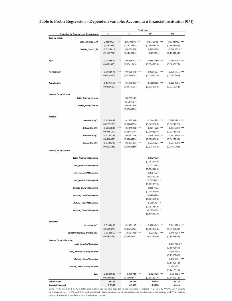
32
Table 6: Probit Regression - Dependent variable: Account at a financial institution (0/1)
(1) (2) (3) (4)
Country Group:
Latin_America (1/0) -0.4583421 ** -0.4194070 ** -0.5673966 *** -0.5549952 ***
(0.181933) (0.1878264) (0.1895855) (0.1993096)
Outside_Comp (1/0) -0.0312811 -0.0252660 0.0505538 -0.2480619 *
(0.1163772) (0.1143764) -0.119894 (0.1384153)
Age 0.0596689 *** 0.0596907 *** 0.0598480 *** 0.0605083 ***
(0.0041873) (0.0041843) (0.0042155) (0.0040979)
Age squared -0.0005675 *** -0.0005679 *** -0.0005697 *** -0.0005771 ***
(0.0000514) (0.0000514) (0.0000517) (0.0000501)
Female (0/1) -0.1277768 *** -0.1100063 ** -0.1260320 *** -0.1262995 ***
(0.0250613) (0.0474025) (0.0251061) (0.0252364)
Country Group*Female
Latin_America*Female -0.0789147
(0.056037)
Outside_Comp*Female -0.0111958
(0.0568383)
Income:
2nd quintile (0/1) 0.1354465 *** 0.1353349 *** 0.1444633 *** 0.1384982 ***
(0.0269293) (0.0268985) (0.0492389) (0.0271176)
3rd quintile (0/1) 0.2853038 *** 0.2849206 *** 0.2914528 *** 0.2875610 ***
(0.0346172) (0.0346076) (0.0492557) (0.0351359)
4th quintile (0/1) 0.4284168 *** 0.4277796 *** 0.4962260 *** 0.4329894 ***
(0.0468422) (0.0468485) (0.0783089) (0.0472038)
5th quintile (0/1) 0.6344226 *** 0.6334404 *** 0.6576324 *** 0.6378588 ***
(0.0492638) (0.0492159) (0.0764781) (0.0499796)
Country Group*Income
Latin_America*2nd quintile 0.0529030
(0.0828447)
Latin_America*3rd quintile 0.1013285
(0.0948265)
Latin_America*4th quintile 0.0567621
(0.087223)
Latin_America*5th quintile 0.2636247 **
(0.1028558)
Outside_Comp*2nd quintile -0.0357772
(0.0642504)
Outside_Comp*3rd quintile -0.0390384
(0.0715009)
Outside_Comp*4th quintile -0.1855474 *
(0.0971332)
Outside_Comp*5th quintile -0.1824519 *
(0.0990047)
Education
Secondary (0/1) 0.5332856 *** 0.5332117 *** 0.5288045 *** 0.3415279 ***
(0.0625379) (0.0625056) (0.0630364) (0.0730049)
Completed tertiary or more (0/1) 1.0526010 *** 1.0524730 *** 1.036217 *** 0.9499514 ***
(0.0783876) *** (0.0784504) (0.078208) (0.1095945)
Country Group*Education
Latin_America*Secondary 0.1677718 *
(0.1009869)
Latin_America*Tertiary or more 0.1106493
(0.1596766)
Outside_Comp*Secondary 0.4089311 ***
(0.1120918)
Outside_Comp*Tertiary or more 0.1582531
(0.1418323)
Cons -2.1895580 *** -2.200715 *** -2.222720 *** -1.968255 ***
(0.6640635) (0.6660247) (0.6611317) (0.6445112)
Observations 96124 96124 96124 96124
Pseudo R-Squared 0.3388 0.3389 0.3398 0.3413
Table 6: Probit Regression - Dependent variable: Account at a financial institution
Controlled for Country Level Determinants
Weak Law
Note: From columns 1 to 4, country level controls are the ones included in the regression of column 7 in table 5. ***,**, and * denote
significance at the 1%, 5%, and 10% level, respectively. Standard errors are in parentheses and are clustered at the country level. The reference
category for education variables is completed primary or less.
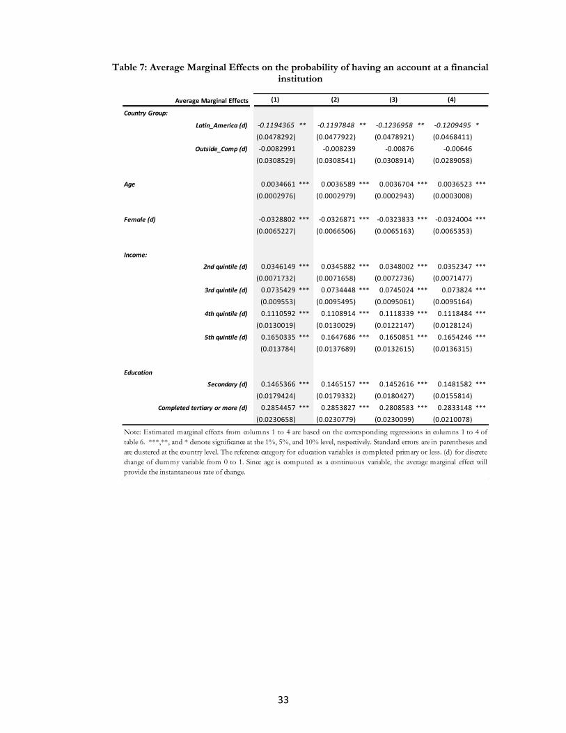
33
Table 7: Average Marginal Effects on the probability of having an account at a financial institution
Average Marginal Effects (1) (2) (3) (4)
Country Group:
Latin_America (d) -0.1194365 ** -0.1197848 ** -0.1236958 ** -0.1209495 *
(0.0478292) (0.0477922) (0.0478921) (0.0468411)
Outside_Comp (d) -0.0082991 -0.008239 -0.00876 -0.00646
(0.0308529) (0.0308541) (0.0308914) (0.0289058)
Age 0.0034661 *** 0.0036589 *** 0.0036704 *** 0.0036523 ***
(0.0002976) (0.0002979) (0.0002943) (0.0003008)
Female (d) -0.0328802 *** -0.0326871 *** -0.0323833 *** -0.0324004 ***
(0.0065227) (0.0066506) (0.0065163) (0.0065353)
Income:
2nd quintile (d) 0.0346149 *** 0.0345882 *** 0.0348002 *** 0.0352347 ***
(0.0071732) (0.0071658) (0.0072736) (0.0071477)
3rd quintile (d) 0.0735429 *** 0.0734448 *** 0.0745024 *** 0.073824 ***
(0.009553) (0.0095495) (0.0095061) (0.0095164)
4th quintile (d) 0.1110592 *** 0.1108914 *** 0.1118339 *** 0.1118484 ***
(0.0130019) (0.0130029) (0.0122147) (0.0128124)
5th quintile (d) 0.1650335 *** 0.1647686 *** 0.1650851 *** 0.1654246 ***
(0.013784) (0.0137689) (0.0132615) (0.0136315)
Education
Secondary (d) 0.1465366 *** 0.1465157 *** 0.1452616 *** 0.1481582 ***
(0.0179424) (0.0179332) (0.0180427) (0.0155814)
Completed tertiary or more (d) 0.2854457 *** 0.2853827 *** 0.2808583 *** 0.2833148 ***
(0.0230658) (0.0230779) (0.0230099) (0.0210078)
Note: Estimated marginal effects from columns 1 to 4 are based on the corresponding regressions in columns 1 to 4 of
table 6. ***,**, and * denote significance at the 1%, 5%, and 10% level, respectively. Standard errors are in parentheses and
are clustered at the country level. The reference category for education variables is completed primary or less. (d) for discrete
change of dummy variable from 0 to 1. Since age is computed as a continuous variable, the average marginal effect will
provide the instantaneous rate of change.
Table 7: Average Marginal Effects on the probability of having an account at a financial
institution

34
53.91
42.88
50.99
38.11
0
10
20
30
40
50
60
Comparators Latin America
Figure 8: Predicted probability of being financially included: By gender
(in percentage points)
male female
44.3
30.2
48.2
34.9
52.2
39.8
57.7
44.0
62.1
53.9
0
10
20
30
40
50
60
70
Comparators Latin America
Figure 9: Predicted probability of being financially included: By income quintiles
(in percentage points)
q1 q2 q3 q4 q5
Note: Figures show predicted probabilities. Calculations are based on probit regressions in table 6 column 3. Source: Authors' calculations based on Findex (2011) database.
Note: Figures show predicted probabilities. Calculations are based on probit regressions in table 6 column 2. Source: Authors' calculations based on Findex (2011) database.

35
5. Conclusions
This paper built on existing research and new databases to address a fundamental question:
What are the relevant factors explaining the observed low ratios of financial inclusion in
Latin America relative to comparable countries in terms of real income per capita? That is,
what explains the Latin American financial inclusion gap?
At the country level we identified four types of obstacles: socio-economic constraints,
macroeconomic vulnerabilities, institutional deficiencies and financial system inefficiencies
that impede the adequate provision of financial services. A key finding of the paper is that,
although the four types of obstacles explain the absolute level of financial inclusion, the
particularly high levels of income inequality and institutional deficiencies in Latin America
can be assessed as the most important obstacles explaining the region’s financial inclusion
gap. These results shed some light on the direction of policies needed to improve the relative
position of Latin America.
Analysis at the individual level, where characteristics such as age, sex, education and
individual income are included, shows that the probability of being financially included is
significantly lower for an individual in Latin America than for someone in comparator
45.22
30.22
55.04
43.92
71.67
59.72
0
10
20
30
40
50
60
70
80
Comparators Latin America
Figure 10: Predicted probability of being financially included: By education level
(in percentage points)
Primary Secondary Tertiary or more
Note: Figures show predicted probabilities. Calculations are based on probit regressions in table 6 column 4. Source: Authors' calculations based on Findex (2011) database.

36
countries. We also found that the relative exclusion of the poorest individuals or those with
the lowest levels of education is higher in Latin America than in comparator countries. As
data on additional individual characteristics become publicly available, further research might
help to obtain the full picture regarding the peculiar features of Latin Americans regarding
financial inclusion and shape the adequate policy responses.

37
References
Acemoglu, D., S. Johnson, and J. A. Robinson (2005). ‘Institutions as a Fundamental Cause of Long-Run Growth’. In Aghion, P. and S. N. Durlauf (eds), Handbook of Economic Growth, Vol. 1A. Amsterdam: Elsevier.
Allen, F., A. Demirgüç-Kunt, L. Klapper and M. Martinez Peria (2012). ‘The Foundations of
Financial Inclusion: Understanding Ownership and Use of Formal Accounts’. Policy Research Working Paper No. 6290. Washington, DC: World Bank.
Beck, T. (2009). ‘The Econometrics of Finance and Growth’. In Mills, T. and K. Patterson
(eds), Palgrave Handbook of Econometrics, Vol. 2. Palgrave Macmillan. Beck, T., A. Demirgüç-Kunt, and P. Honohan (2008). ‘Finance for All? Policies and Pitfalls
in Expanding Access’. Policy Research Report. Washington, DC: World Bank. Beck, T., A. Demirgüç-Kunt, and R. Levine (2007). ‘Finance, Inequality and the Poor’.
Journal of Economic Growth, 12, 27-49. Beck, T., A. Demirgüç-Kunt, and M. Martinez Peria (2006). ‘Banking Services for Everyone?
Barriers to Bank Inclusion and Use around the World’. World Bank Policy Research Working Paper No. 4079. Washington, DC: World Bank.
Beck, T., A. Demirgüç-Kunt, and M. Martinez Peria (2005). ‘Reaching Out: Inclusion to and
use of Banking Services across Countries’. World Bank Policy Research Paper No. 3754. Washington, DC: World Bank.
Beck, T., A. Demirgüç-Kunt, and V. Maksimovic (2003). ‘Bank Competition, Financing
Obstacles and Inclusion to Credit’. World Bank Policy Research Paper No. 2996. Washington, DC: World Bank.
Beck, T., A. Demirgüç-Kunt, R. Levine, M. Cihak, and E. H.B. Feyen. ‘A New Database on
Financial Development and Structure’. (Updated 2012). World Bank Economic Review 14, 597-605.
Behrman, J., N. Birdsall, and G. Petterson (2009). ‘Schooling Inequality, Crises and Financial
Liberalization in Latin America’. CGD Working Paper No. 165. Washington, DC: Center for Global Development.
Birdsall, N., N. Lustig, and C. Meyer (2013). ‘The New Poor in Latin America: Challenges
and Risks’. Center for Global Development. Brune, L., X. Giné, J. Goldberg, and D. Yang (2011). ‘Commitments to Save: A Field
Experiment in Rural Malawi’. World Bank, Policy Research Working Paper No. 5748. Washington, DC: World Bank.
CAF (2011). ‘Servicios Financieros para el Desarrollo: Promoviendo el Acceso en América
Latina’. Bogota, April. Calderon, C., and A. Chong (2001). ‘External sector and income inequality in independent
economies using a dynamic panel data approach’. Economic Letters, 71(2), 225-231.

38
Claessens, S., and L. Leaven (2003). ‘Financial development, property rights, and growth’. Journal of Finance, 58(6), 2401–2436.
Claessens, S. (2005). ‘Universal Inclusion to Financial Services: A Review of the Issues and
Public Policy Objectives’. OECD-World Bank, Fifth Services Experts Meeting. OECD, Paris, February.
Claessens, S., and E. Perotti (2005). ‘The Links between Finance and Inequality: Channels
and Evidence’. University of Amsterdam, March. Clarke, G., L. Colin Xu, and H. Zou (2006). ‘Finance and Inequality: What Do the Data Tell
Us?’. Southern Economic Journal, 72(3): 578–96. Demetriades, P., and S. Andrianova (2004). ‘Finance and Growth: What We Know and
What We Need to Know’. In C. Goodhart (eds), Financial Development and Economic Growth: Explaining the Links, 38-65. Palgrave Macmillan: Basingstoke and New York.
Demirgüç-Kunt, A., and R. Levine (2008). ‘Finance and Economic Opportunity’. World
Bank Policy Research Paper No. 4468. Washington, DC: World Bank. Dupas, P., and J. Robinson (2009). ‘Savings Constraints and Microenterprise Development:
Evidence from a Field Experiment in Kenya’. NBER working paper No. 14693. Ferreira, F., J. Messina, J. Rigolini, L. López-Calva, M. Lugo, and R. Vakis (2012).
‘Economic Mobility and the Rise of the Middle Class in Latin America’. The World Bank.
Gratius, S. (2008). ‘The International Arena and Emerging Powers: Stabilizing or
Destabilizing Forces?’. Comment, FRIDE, April. Honohan, P. (2007). ‘Cross-Country Variation in Household Access to Financial Services’.
The World Bank, January. Latin America Shadow Financial Regulatory Committee (2004). ‘Small and Medium-Size
Enterprises in Latin America: Developing Markets, Institutions and Instruments’. Statement No, 11. Washington, DC, September.
Levine, R. (2005). ‘Finance and Growth: Theory and Evidence’. In Aghion, P. and S. Durlauf (eds), Handbook of Economic Growth. Elsevier Science. The Netherlands.
Lopez-Calva, L. and E. Ortiz-Juarez (2011). ‘A Vulnerability Approach to the Definition of
the Middle Class’. World Bank, Policy Research Working Paper No. 5748. Washington, DC: World Bank.
Martínez Pería, M. (2012). ‘Financial Inclusion: Where does LAC stand?’. In De la Torre, A.,
Ize, A. and Schumkler, S. (eds), Financial Development in Latin America and the Caribbean, The Road Ahead. World Bank, Flagship Report. Washington, DC: World Bank.
Milanovic, B. (2010). ‘The Haves and the Have-Nots: A Brief and Idiosyncratic History of
Global Inequality’. New York: Basic Books.

39
Pritchett, L. (2010). ‘Birth Satisfaction Units (BSU): Measuring Cross-National Differences in Humal Well-Being’. United Nations Development Program, Research Paper 2010/03, Human Development Reports, June.
Rojas-Suarez, L. (2007). ‘The Provision of Banking Services in Latin America: Obstacles and
Recommendations’. CGD Working Paper No. 124. Washington, DC: Center for Global Development.
Rojas-Suarez, L. (2009). ed. ‘Growing Pains in Latin America: An Economic Growth
Framework as Applied to Brazil, Colombia, Costa Rica, Mexico and Peru’, Center for Global Development, July.
Rojas-Suarez, L. and V. Gonzales (2010). ‘Inclusion to Financial Services in Emerging
Powers: Facts, Obstacles and Policy Implications’. OECD Development Centre, March. Singh, A., A. Belaisch, C. Collyns, P. de Masi, R. Krieger, G. Meredith and R. Rennhack
(2005). ‘Stabilization and Reform in Latin America: A Macroeconomic Perspective on the Experience Since the Early 1990s’. IMF Occasional Paper No. 238, February.
Wilson, D. and A. Stupnytska (2007). ‘The N-11: More than an Acronym’. Global Economic
Papers No. 153, Goldman Sachs, March 28. ----- (2003). ‘Dreaming with BRICs: The Path to 2050’. Global Economics Paper No. 99,
Goldman Sachs, October.

40
Annex I: Grouping of countries by category
Latin America(1) Latin American comparators High Income countries Rest of the world
Argentina Albania Indonesia Saudi Arabia Australia Kuwait Afghanistan Lesotho Tajikistan
Bolivia Algeria Iran, Islamic Rep.
Slovak Republic
Austria Luxembourg Bangladesh Liberia Togo
Brazil Angola Jamaica South Africa Bahrain Malta Benin Madagascar Uganda
Chile Armenia Jordan Sri Lanka Belgium Netherlands Burundi Malawi West Bank and Gaza
Colombia Azerbaijan Kazakhstan Swaziland Canada New Zealand
Cameroon Mali Yemen, Rep.
Costa Rica Belarus Latvia Syrian Arab Republic
Cyprus Oman Central African Republic
Mauritania Zambia
Ecuador Bosnia and Herzegovina
Lebanon Thailand Denmark Portugal Chad Mongolia Zimbabwe
El Salvador Botswana Lithuania Tunisia Finland Qatar Comoros Mozambique
Guatemala Bulgaria Macedonia, FYR
Turkey France Singapore Congo, Dem. Rep.
Nepal
Honduras China Malaysia Turkmenistan Germany Slovenia Ghana Niger
Mexico Congo, Rep. Mauritius Ukraine Greece Spain Guinea Nigeria
Nicaragua Czech Republic
Montenegro Uzbekistan Hong Kong, China
Sweden Haiti Rwanda
Panama Djibouti Morocco Ireland Trinidad and Tobago
India Senegal
Paraguay Estonia Philippines Israel United Arab Emirates
Iraq Sierra Leone
Peru Gabon Poland Italy United Kingdom
Kenya Somalia
Uruguay Georgia Romania Japan United States
Kyrgyz Republic
Sudan
Hungary Russian Federation
Korea, Rep.
Lao PDR Taiwan, China
(1)We have removed Venezuela from the sample because it is an outlier based on the studentized residuals criterion.
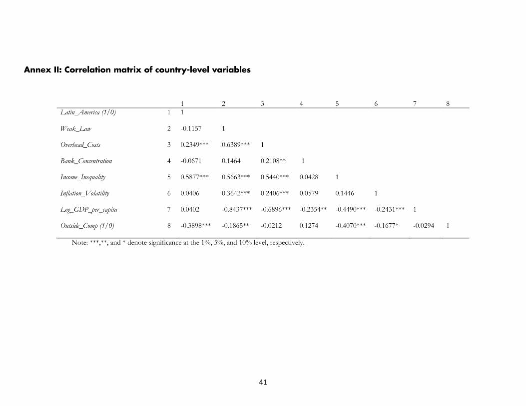
41
Annex II: Correlation matrix of country-level variables
1 2 3 4 5 6 7 8
Latin_America (1/0) 1 1
Weak_Law 2 -0.1157 1
Overhead_Costs 3 0.2349*** 0.6389*** 1
Bank_Concentration 4 -0.0671 0.1464 0.2108** 1
Income_Inequality 5 0.5877*** 0.5663*** 0.5440*** 0.0428 1
Inflation_Volatility 6 0.0406 0.3642*** 0.2406*** 0.0579 0.1446 1
Log_GDP_per_capita 7 0.0402 -0.8437*** -0.6896*** -0.2354** -0.4490*** -0.2431*** 1
Outside_Comp (1/0) 8 -0.3898*** -0.1865** -0.0212 0.1274 -0.4070*** -0.1677* -0.0294 1
Note: ***,**, and * denote significance at the 1%, 5%, and 10% level, respectively.

42
Annex III: Additional Variables included in the preliminary estimations
Variable Description Source Available years
Non performing loans to total loans
Bank nonperforming loans to total gross loans are the value of
nonperforming loans divided by the total value of the loan
portfolio (including nonperforming loans before the deduction
of specific loan-loss provisions). The loan amount recorded as
nonperforming should be the gross value of the loan as
recorded on the balance sheet, not just the amount that is
overdue.
World Bank (WB) 2000-2011
Bank Provisions to non performing Loans Financial Soundness Indicators (IMF) 2005-2010
Regulatory capital to risk weight assets Financial Soundness Indicators (IMF) 2005-2010
Bank Capital to Assets Financial Soundness Indicators (IMF) 2005-2011
Liquidity Ratio Bank liquid reserves to bank assets ratio (%) WB 2001-2011
Banking assets held by government-owned
banks (% of total banking assets)-2005Barth, Caprio and Levine database 2005
Lending Interest Rate WB 1960-2010
Deposit Interest Rate WB 1960-2010
Interest rate spread WB 1960-2010
Net interest marginAccounting value of bank's net interest revenue as a share of its
interest-bearing (total earning) assets.Fitch's BankScope database 1987-2009
BANK ROA Fitch's BankScope database 1960-2009
BANK ROE Fitch's BankScope database 1960-2009
volatility of gdp growth 1990-2000/2001-2011 World Economic Outlook database (IMF)
GDP acceleration (2000s vs 1990s)average of gdp growth (2011-2001) minus average gdp growth
(2000-1990)
Authors' calculations based on World Economic
Outlook database (IMF)
Poverty ratio %
PovcalNet: the on-line tool for poverty
measurement developed by the Development
Research Group of the World Bank'
http://iresearch.worldbank.org/PovcalNet/ind
ex.htm?2
various
Rural population (% of total population) World Development Indicators (WDI) 1960-2010
Doing Business, legal right index
Strength of legal rights index measures the degree to which
collateral and bankruptcy laws protect the rights of borrowers
and lenders and thus facilitate lending. The index ranges from 0
to 10, with higher scores indicating that these laws are better
designed to expand access to credit.
Doing Business 2004-2011
Doing Business, credit information index
Credit depth of information index measures rules affecting the
scope, accessibility, and quality of credit information available
through public or private credit registries. The index ranges
from 0 to 6, with higher values indicating the availability of
more credit information, from either a public registry or a
private bureau, to facilitate lending decisions.
Doing Business 2004-2011
Heritage Financial Freedom Index
The Index scores an economy’s financial freedom by looking
into the following five broad areas: The extent of government
regulation of financial services, The degree of state intervention
in banks and other financial firms through direct and indirect
ownership, The extent of financial and capital market
development, Government influence on the allocation of credit,
and Openness to foreign competition
Heritage 1995-2012

43
Annex IV: Validity of Instruments in the Endogeneity Analysis
The relevance of the instruments is analyzed through the statistics of the first stage
regression in Table IV.I. The R-squared and the adjusted R-squared are around 0.7, which
means that there won’t be significant loss of precision because of IV estimation. Also, both
instruments are significant when explaining Income_Inequality, controlling for the remaining
obstacles (excluded instruments).
Table IV.I: OLS Regression - First-stage regression
Dependent variable: Income Inequality
(1)
Latin America (1/0) 8.71101 ***
(1.713146)
Weak law 0.088894
(0.1155747)
Overhead cost 0.467423
(0.3515685)
bank concentration 0.0527601
(0.0871163)
bank concentration*weak_law 0.0012515
(0.0015521)
Trade Openness -0.0579027 ***
(0.0209949)
Trade Openness*Trade_Concentration 0.105755 **
(0.0456942)
Inflation Volatility -1.717728 ***
(0.5982767)
Outside Comparators (1/0) -4.145863 **
(1.651272)
Cons 48.86809 ***
(6.610664)
Observations 90
R-squared 0.7034
Adjusted R-squared 0.6700
Note: ***,**, and * denote significance at the 1%, 5%, and 10% level,
respectively. Robust standard errors are in parentheses.
Table IV.I: OLS Regression – First-stage regression Dependent variable: Income Inequality

44
The exclusion restriction is also fulfilled. Table IV.II column 1 shows the OLS estimation
of equation (1) controlling simultaneously for Income_Inequality and the corresponding
instruments. Under this specification, both instruments are not significant in explaining
financial inclusion. However, when removing Income_Inequality, Trade_Openness becomes
significant and its interaction term is very close to be significant48 (see column 2). This
exercise supports the argument that the effect of the instruments on financial inclusion is
only through their effect on Income_Inequality.
48 Statistically significant at the 18% level.
Table IV.II: Regression - Dependent variable: Financial Inclusion Ratio (2011)
(1) (2)
Latin America (1/0) -8.05355 -10.42202 **
(5.053559) (4.867017)
Weak_Law -0.757209 *** -0.820972 ***
(0.2100573) (0.1991836)
Overhead_Costs -1.164410 -1.540701 *
(1.061411) (0.8578353)
Bank_Concentration -0.3411860 * -0.3927155 **
(0.1783621) (0.1655031)
Bank_Concentration*Weak_Law -0.0044996 0.0050765 *
(0.0028479) (0.0026924)
Income_Inequality -0.5340706 *
(0.3022005)
Trade_Openness 0.0249903 0.0527909 *
(0.0361353) (0.0322554)
Trade_Openness*Trade_Concentration -0.062706 -0.145660
(0.1035126) (0.1085976)
Inflation_Volatility -3.354288 * -1.397752
(1.757216) (1.535763)
Outside_Comp (1/0) -5.053559 0.142222
(4.275802) (3.770228)
Cons 51.47901 ** 23.90974 *
(19.83234) (12.65929)
Observations 90 111
R-squared 0.8197 0.7924
Table IV.II: OLS Regression - Dependent variable: Financial
Inclusion Ratio (2011)
Note: ***,**, and * denote significance at the 1%, 5%, and 10% level, respectively.
Robust standard errors are in parentheses.

45
Annex V: Results under an Alternative Definition of the Financial Inclusion Gap (Latin America relative to High Income
countries)
Table V.I: OLS Regression - Dependent variable: Financial Inclusion Ratio (2011)
(1) (2) (3) (4) (5) (6) (7)
Latin_America (1/0) -60.23311 *** -26.00768 *** -23.48866 *** -26.37723 *** -27.62997 *** -19.06786 ** -18.97034 **
(3.564747) (5.81143) (6.128063) (6.219678) (5.96395) (7.33746) (7.282937)
Weak_Law -1.031015 *** -0.897276 *** -0.861673 *** -0.413902 ** -0.479442 ** -0.420305 *
(0.1183783) (0.1232726) (0.1313036) (0.1918728) (0.2153179) (0.2217809)
Overhead_Costs -2.061473 ** -1.605704 * -1.380773 -1.993904 * -1.897226 *
(0.9087449) (0.9103235) (0.9078429) (1.149645) (1.104352)
Bank_Concentration -0.1751761 * -0.5405857 *** -0.4490912 ** -0.4478388 **
(0.0734331) (0.1558478) (0.1734661) (0.1674374)
Bank_Concentration*Weak_Law -0.0073595 *** -0.0063791 ** -0.0063449 **
(0.0025373) (0.0026718) (0.0026211)
Income_Inequality -0.3312317 -0.3445690
(0.2597597) (0.2571944)
Inflation_Volatility -3.147173 *
(1.652687)
Log_GDP_per_capita
Outside_High_income (1/0) -54.451110 *** -17.337270 *** -15.91417 *** -17.15868 *** -17.92617 *** -12.13076 * -12.35295 **
(3.359178) (5.076848) (5.212547) (5.522648) (5.32658) (5.533436) (5.592893)
Cons 89.32686 *** 11.87579 24.76691 ** 37.18776 *** 59.66467 *** 65.42503 *** 72.29192 ***
(2.003171) (9.172523) (10.05539) (12.01966) (13.98804) (19.22661) (20.2336)
Observations 137 136 125 119 119 94 93
Adjusted R-squared 0.5564 0.7502 0.7645 0.7824 0.7904 0.8056 0.8203
Note: ***,**, and * denote significance at the 1%, 5%, and 10% level, respectively.
Robust standard errors are in parentheses.
Weak Law
Table V.I: OLS Regression - Dependent variable: Financial Inclusion Ratio (2011)