working paper 182 - rising food prices and household ... food prices and household welfare in...

Rising Food Prices and Household Welfare in Ethiopia:

Evidence from Micro Data

Abebe Shimeles and Andinet Delelegn

No 182 – September 2013

Correct citation: Shimeles A. and Delelegn A. (2013), Rising Food Prices and Household Welfare in Ethiopia:

Evidence from Micro Data Working Paper Series N° 182 Rising food prices and household welfare in Ethiopia:

evidence from micro data.

Steve Kayizzi-Mugerwa (Chair)

Anyanwu, John C.

Faye, Issa

Ngaruko, Floribert

Shimeles, Abebe

Salami, Adeleke

Verdier-Chouchane, Audrey

Coordinator

Working Papers are available online at

http:/www.afdb.org/

Copyright © 2013

African Development Bank

Angle de l’avenue du Ghana et des rues Pierre de

Coubertin et Hédi Nouira

BP 323 -1002 TUNIS Belvédère (Tunisia)

Tel: +216 71 333 511

Fax: +216 71 351 933

E-mail: [email protected]

Salami, Adeleke

Editorial Committee Rights and Permissions

All rights reserved.

The text and data in this publication may be

reproduced as long as the source is cited.

Reproduction for commercial purposes is

forbidden.

The Working Paper Series (WPS) is produced by

the Development Research Department of the

African Development Bank. The WPS disseminates

the findings of work in progress, preliminary

research results, and development experience and

lessons, to encourage the exchange of ideas and

innovative thinking among researchers,

development practitioners, policy makers, and

donors. The findings, interpretations, and

conclusions expressed in the Bank’s WPS are

entirely those of the author(s) and do not

necessarily represent the view of the African

Development Bank, its Board of Directors, or the

countries they represent.

Rising Food Prices and Household Welfare in Ethiopia:

Evidence from Micro Data

Abebe Shimeles and Andinet Delelegn1

ABSTRACT

1 Abebe Shimeles and Andinet Delelegn are respectively Manager at the Development Research Department,

African Development Bank and Lecturer at the Department of Economics, Georgian State University. The

authors are grateful to Arne Bigsten, Jeni Klugman, Joseph Loeing, Paul Dorosh and members of the Ethiopian

Inflation Study Task Force for very useful comments and suggestions.

AFRICAN DEVELOPMENT BANK GROUP

Working Paper No. 182

September 2013

Office of the Chief Economist

This paper analyzes welfare implications of

rising commodity prices in Ethiopia based

on household budget surveys. Our findings

suggest that a rise in relative prices of such

necessities as cereals would lead to a large

deterioration in the welfare of households in

urban areas. In rural areas generally land-

rich households tend to benefit significantly

from the recent surge in food prices, while

the land-poor and typical farm households

tend to experience negative growth. Thus,

price shifts in favour of agriculture could

aggravate poverty conditions in rural areas.

Simulated Gini computed from simple

demand systems indicate worsening income

distribution in urban areas due to price

shifts that would exacerbate the already

dire poverty conditions. The paper also

reported own and cross-price elasticities

mainly for cereals to gain insight into

magnitude of demand shifts due to income

and price changes.

5

1. Introduction

The Ethiopian economy has witnessed a double-digit rate of inflation since 2003, culminating

at 53% in June 2008. Particularly the significant rise in the relative prices of grain and other

foodstuff such as sugar, edible oil and other necessities in recent period are very worrisome.

Evidently such large changes in both absolute and relative prices in a space of few years can

undermine the rebound in per capita incomes in the last decade and the poverty reduction

effort of the government.

The gravity of the problem has been well understood by policy makers, and efforts are

underway to cushion vulnerable households from the consequences of the price surge. The

potential role of such interventions can only be known if welfare effects of rising prices are

understood. In addition, better measures of the key parameters that drive the demand for grain

and other goods is a useful input to the analysis of the causes of relative price changes in

Ethiopia.

This paper attempts to fill some of the gaps in our knowledge of the link between welfare and

rising prices by examining first what the distributional consequence of the rise in absolute

price has been over the recent period in rural as well as urban areas. It provides quantitative

estimates of the change in the measure of income inequality due to price changes alone. Such

findings will indicate whether or not the poor have been affected relatively more than others

during an inflationary period. Secondly, the study provides evidence on the welfare

implications of changes in relative prices of key consumption goods by constructing

concentration curves using non-parametric methods. The pair-wise comparison of

concentration curves provides a useful analytical framework in generating partial ordering of

welfare between consumption goods. This framework can be also used to analyze whether

subsidies on wheat or other grain products could raise welfare, particularly so if it is financed

through surtax imposed on other commodities, or income. Third, the paper estimates the

effect of changes in the relative prices of agricultural goods on consumption growth for rural

as well as urban households to capture welfare effects of the price shocks. Finally, a range of

income and cross-price elasticity of demand values are reported to understand better the role

of demand shifts in driving relative price changes. The key results emerging from our

analysis are first, the recent dramatic rise in the general price could be responsible in raising

the average Gini coefficient in urban areas by more than 2% every year. In other words,

between 2000 and 2006, the Gini coefficient could rise by about 6 percentage points due to

inflation alone suggesting the anti-poor bias the inflationary process has in urban areas.

Secondly, consumption pattern for cereals and other food items suggest that subsidies

targeted at maize in rural areas, and teff in urban areas financed say through a proportional

income tax (surtax) could be welfare enhancing, particularly for the poor population. Finally,

while real consumption growth deteriorated significantly following the rise in the real price

of food (cereals) in urban areas, its effect on rural households depends on the potential to be

net seller or buyer. As a result, land rich households tend to benefit significantly from real

and nominal price movements of cereals while land poor households lose enormously. Thus,

policy reforms designed to raise agricultural terms of trade in favour of the rural sector need

to bear in mind that it has the potential to precipitate poverty by impoverishing the land-poor

and consequently raising income inequality as well as pushing the average farm household

into poverty.

6

The next section discusses in some detail the methodological framework used in the paper,

Section 3 describes the data source and survey methodology, Section 4 discusses key results

and Section 5 concludes the paper.

2. Methodological framework

2.1. Welfare implications of inflation

To establish empirically the impact of inflation on the poor, it is possible to use two

approaches (though interrelated) based on household budget surveys. The first, and perhaps

simplest, is incidence analysis using concentration curves for a wide range of commodities.

In this case, the rise in price of a particular commodity is regarded as an implicit tax, and the

expenditure profile of this commodity (or sets of commodities) is used to infer whether the

rise in price affects poor households differently from non-poor ones. This exercise provides

rich information on the aggregate welfare implications of increase in commodity prices and

its distributional implications (see eg. Yitzhaki and Slemrod 1991). Furthermore, this

approach allows for evaluating the welfare consequence of subsidizing a wide range of

commodities.

Concentration curves are generalized forms of the popular summary distributional measure

known as the Lorenz curve. The distribution of expenditure on various goods across a

spectrum of household characteristics renders valuable insights to policy options2. The

concept of concentration curves was first used by Roy, et al (1959); and later Kakwani (1980)

provided proof of some of the empirical properties, and Yithaki and Slemrod (1991) used

them to analyze issues of marginal tax reform in a revenue-neutral setting.

As defined by Yitzhaki and Slemrod (1991: 481), "the concentration curve is a diagram

similar to the Lorenz curve. On the horizontal axis, the households are ordered according to

their income, while on the vertical axis describes the cumulative percentage of the total

expenditure on specific commodity that is spent by the families whose incomes are less than

or equal to specified income level". This definition of a concentration curve embodies the

income effects; and Rao et al (1959) introduced relative concentration curves to normalize

the effects of differences in purchasing power so that the effect of differences in preferences

for various commodities can be neatly captured. Kakwani (1980)3 proved important theorems

pertaining to concentration curves of which the following may be reproduced for the purpose

of this paper:

i. If the income elasticity of commodity i, Ei is greater than the income elasticity of

commodity j, then, the concentration curve for i lies above the concentration curve for

j;

ii. The concentration curve for commodity i will be above (below) the egalitarian line

if, and only if Ei is less (or greater) than zero for all income level greater than zero.

2 see also Haggablade and Younger (2003), and Younger et al, (1999) for the application of concentration curves

on African data and Michael (2003) on Ethiopia. Early attempt on Ethiopia using the 1980/81 household income

and consumption survey was made by Shimeles (1993)

3Kakwani (1980), op cit, pp165-166.

7

iii. The concentration curve for commodity i lies above (below) the Lorenz curve if,

and only if , Ei is less (greater) than unity for all income greater than zero.

It follows therefore, that if the concentration curve of a commodity lies above the 450 line, it

is an inferior commodity, if the concentration curve lies between the Lorenz curve and the

450 line, it is a necessary commodity, and if the concentration curve lies below the Lorenz

curve, the commodity is luxury.

Yitzhaki and Slemrod (1991) made an insightful use of concentration curves in the realm of

public economics to analyze issues of tax reform. It is rather becoming conventional in the

literature to look into the structure of indirect tax systems, and the possibility of reform by

maximizing social-welfare function of the community subject to a government revenue

constraint4. This approach presupposes the knowledge of Indirect Utility Function of the

community, and thus the respective demand systems in order to be of any empirical use.

When one looks at the severe limitations that developing countries face to meet the data

requirements of this approach, then, the search for an alternative method remains a very

compelling one. In this respect, the Marginal Conditional Stochastic Dominance Rules

(MCSD) developed by Yithaki and Smlerod (1991) using the concept underlying

concentration curves can be considered as a significant step to that end. MCSD is defined as a

state where " if the (shifted) [due to tax incidence] concentration curve of one commodity is

above the (shifted) concentration curve of another commodity, then, the first commodity

dominates in the sense that a small tax decrease in the first commodity accompanied by a taxi

increase in the second (with revenue remaining unchanged) increases social welfare

functions. In other words, if and only if concentration curves do not intersect will all additive

social-welfare functions show that the tax change increases welfare. We refer to these rules as

Marginal Conditional Stochastic Dominance Rules"5. Normally this proposition would have

required the plotting of n(n-1)/2 curves, which for a sufficiently large number of commodities

becomes cumbersome. The Gini-coefficient has been used to identify a class of easily

computable necessary conditions for welfare dominance via the translation into income

elasticities. This condition states that the income elasticity of commodity i should be lower

than that of commodity j in order for commodity i to dominate commodity j in the event they

are subject to an indirect tax.

We may show the above relations explicitly using the concentration ratio or index concept,

which is defined as one half of the area below the 450

line minus the concentration curve.

That is,

i

ii

m

yFXCovc

)](,[ (1)

Where, ci is one-half of the concentration ratio, mi is the mean expenditure on commodity i,

Xi is total expenditure on commodity i, and F (y) is the cumulative distribution of income.

4see Atkinson (1970) for the specification of a social-welfare function, Ahmad And Stern (1984), King (1983),

Cragg (1991) for empirical application and Deaton (1979, 1981) for the implication of additive preferences to

optimal commodity taxes.

5Yitzhaki and Smelord (1991), op cit, pp 482

8

Therefore, the area between the concentration curve of commodity i, and the concentration

curve of commodity j can be written as:

y

j

j

i

iji G

S

b

S

bcc ][ (2)

Where,

)](,[

)(,(

yFyCov

yFXCovb i

i

y

ii

m

mS

And my stands for mean income or expenditure. Here the revenue implication of the policy

reform is assumed to be neutral that is there is no gain or loss to the government. We may

interpret bi/Si as the weighted average income elasticities of commodity i, the weight being

here the Gini-coefficient-implied welfare function, and is a nonparametric estimator of the

slope of the regression line of Si on y.6 Thus for commodity i to dominate commodity j the

weighted income elasticity of commodity i should be larger than for commodity j. The

weighting scheme employed here is the Gini-index which also implies a specific form of

social-welfare function. In fact, we can further broaden the weighting scheme by using the

notion of the extended Gini index , which is given by:

ym

yFyCovG

1)](1,[)(

where, G () is a parameter chosen by the investigator. The Gini is a special case of G ()

where, is 2. The higher is the greater is the emphasis on the bottom of the income

distribution.

2.2. Demand systems and household welfare

A related approach is to construct a simple demand system for the commodities of interest

and use the direct link between expenditure shares and Gini coefficients to quantify the

extent to which the rise in prices has impacted on the overall Gini coefficient (Kakwani,

1980). From this exercise it would be possible to tell whether the inflationary process is

against the poor, distribution neutral or biased against well off households. The basic

framework is that of the Stone-Greary utility function that gives the Linear Expenditure

Systems, which is given by:

)(1

k

k

khtiitihtiti pypxp

(3)

6see Yitzhaki and Slemrod (1991), op cit , pp 487.

9

Where pit is price of commodity i prevailing at period t, xit is quantity of i demanded by

household h at period t, yht is total income of household h at period t and i and i are

parameters to be estimated, representing respectively the “subsistence” consumption of

commodity i, and i is the marginal budget share. The structure of the LES is motivated by

the assumption that regardless of income levels, each household allocates its income first on

subsistence goods and the remaining is driven by consumption preference. Estimation of (2)

is complicated by the non-linear term linking marginal budget share with the

“supernumerary” income or consumption expenditure so that a numerical approximation is

used in the context of non-linear system of equations. Despite some limitations, the LES

provides a simple framework to capture the welfare implications of changes in relative prices.

Estimation of (3) from one cross-section data can be made using additional information on

consumption decision, such as savings. For instance, it is possible to establish whether

inequality of income changes due to changes in relative prices. To do that we use the result in

Kakwani (1980) that links Gini coefficient between two price settings on the assumption that

real income among households is held constant:

1 1 1

*

*

1

00

*

))((i i i i

iiitii

i i

i

ti

i

p

ppp

Gp

p

G

(4)

Where Gt is Gini coefficient at period t with price vector P*, t is mean consumption

expenditure at period t and 0 is mean consumption expenditure in period 0. Using estimated

coefficients from (3), it is possible to compute the Gini coefficient at the new set of prices

and examine whether or not it leads to a worsening state. The LES is less attractive to

investigate price responses though.

A better framework to estimate price elasticities for a wide range of commodities, such as

teff, wheat, and maize would be flexible demand functional form such as the Almost Ideal

Demand System (AIDS) of Deaton and Mullebauer (1980), which is given as follows:

)/log(log PXpw ij

j

ijii (5)

Where: wi is the ith

budget share, pj is prices of commodity j, δ is the price coefficient and β

is the income coefficient of demand for commodity i and P is a price index that is implicitly

defined by logP as in equation 2:

jk

j k

kj

k

kk PPPP loglog2

1loglog 0 (6)

Demand theory imposes structure on equation (1) by assuming that demand function is

homogenous of degree 1 in prices and income, and that price responses are symmetric across

commodities. These assumptions lead to the following well known restrictions:

10

1 i , 0 ij , 0 i , jiij

Several approximations have been suggested in the empirical literature to consistently

estimate the system of demand equations given by (1) due to complexities involved in

equation (5)7. Following Hayes et al (1990) we use the Laspeyers index to estimate equation

2 which is given by :

k

kk PwP loglog (7)

A linear approximation of the relevant elasticties is also given by the following equations:

Own-price elasticities:

)1()/( iiiiii w (8)

Cross-price elasticities:

j

i

i

i

ij

ij www

(9)

The income elasticities

1i

ii

w

(10)

Compensated (Hicksian) elasticity of demand is given by:

ijijij w *

To address possibility of non-linearity in expenditure functions, we complement our

estimation with a quadratic specification of the AIDS model that is frequently used in applied

work (see for example, Banks et al, 1997 for the derivation of quadratic AIDS model; and

Bopape and Myers, 2007, Tasciotti, 2007 for recent applications). The quadratic AIDS

demand system is given by:

])(

[log)()(

loglog

2

pP

x

pbpP

xpw ijijii

(11)

where,

kpPb 0)(

ji

i j

ijii pppaPa loglog2

1log)(log 0

Estimates of the appropriate own and cross price elasticities, as well as, the income

elasticities is reported for equation (11) as a further test of robustness of the lineraized AIDS

specification.

7 In this study we use log-linerarized version of the AIDS model especially to approximate equation (3).

11

In addition to non-linearities involved in the estimation of the AIDS model, there are a

number of other issues such as censoring of the expenditure data due to zero observations that

pose econometric challenges. Parameter estimates are controlled for selectivity bias due to

censoring. The censoring issue further complicates the soundness of the theoretical

restrictions outlined above, like symmetry, adding-up and homogeneity assumptions. In this

study we address some of the empirical issues, such as non-linearities in expenditure

functions, of estimating a consistent price and income responses by a typical household.

3. Data

The data for this study comes from two sources. The first is the panel data set collected by

Addis Ababa University in collaboration with Oxford University for rural areas and

University of Gothenburg for urban areas covering the period 1994-2004 in five waves. This

data set contains most of the variables of interest here. The sample is 3,000 households

divided equally between urban and rural areas where nearly 90% of households for rural and

60% for urban have been interviewed in all waves. In the rest of the cases, appropriate

replacements have been made. Thus, the unbalanced data consists of approximately the

history of 3000 households in five waves. The second data set is the 1999/2000 Household

Income and Consumption Expenditure Survey (HICES) of the CSA, which covered a

nationally representative sample of 17000 households with variables on income, consumption

expenditure, household demographics and others useful for welfare analysis.

The panel data set originally consisted of approximately 3000 households, equally divided

between rural and urban areas. The nature of the data, the sampling methods and other

features are discussed in detail in Bigsten et al. (2005). It is one of the few longitudinal data

sets available for Africa. The data covers households’ livelihoods, including asset

accumulation, labor market participation as well as health and education and other aspects of

household level economic activities.

The common problem in using consumption expenditure for welfare analysis is that of

measurement errors. The major source of errors could come from problems associated with

accurate reporting during data collection, which in general has to do with the level of

disaggregation of consumption baskets. The finer the consumption breakdown the better is

the accuracy of measurement (e.g. Deaton, 1997). In our case, the consumption breakdown is

very detailed, and has been held constant to allow inter-temporal comparisons. In computing

consumption expenditures, we used quantities reported for each commodity by respondents

and per unit prices from the nearby market. However, major food expenses among

households in Ethiopia are difficult to measure, particularly in rural areas, because of

problems related to measurement units, prices, and quality. The consumption period could be

a week or a month depending on the nature of the food item, the household budget cycle, and

consumption habits. Own-consumption is the dominant source of food consumption in rural

Ethiopia, particularly with regard to vegetables, fruits, spices and stimulants like coffee and

chat.8 Cereals, which make up the bulk of food consumption, is increasingly obtained from

markets as farmers swap high cash-value cereals such as teff for lower-value ones, such as

maize and sorghum. In the urban setting, the bulk of consumption items are obtained from

markets and measurement problems are less. To address this issue, we used carefully

8 Chat is a stimulant leaf commonly used in Ethiopia and neighboring countries.

12

constructed conversion factors for all types of commodities that are comparable across

households.

There may also be other sources of error that are systematic across households (say better

educated households could be relatively better at keeping records of their regular expenses),

or across survey periods (seasonality effects). So, consumption expenditure is not immune to

measurement error even in the best-administered surveys.

4. Discussion of results

4.1. Incidence analysis of the welfare impact of inflation

As described in Section 2, the pattern of consumption could provide important information on

how changes in the relative prices of consumption goods might affect welfare across a cross-

section of households. In this section, we discuss results based on the behaviour of

concentration curves for a wide range of commodities to investigate two key issues. The first

examines the distributional consequence of changes in the relative price of commodities. The

second issue deals with welfare implications of possible government interventions through

price supports financed mainly by raising taxes on commodities or income. Concentration

curves for a wide range of commodities have been constructed for rural and urban households

separately. To compare results, we have used the nationally representative income and

expenditure survey of the CSA, 1999, focusing on urban households

To get a sense of the profile of consumption, Table A1 and Table A2 report detail profile of

consumption expenditure by consumption quintile and rounds. It can be inferred from these

tables that monthly total expenditure on consumption between 1994 and 2004 is devoted

largely to food and drinks, as one might expect in a poor economy such as Ethiopia. Thus,

changes in prices of food and drinks relative to non-food consumption items can have

significant effects on consumption growth, an issue that will be taken up in great detail

below. Among food items, cereals account in rural areas about 42% and in urban areas 22%

of total consumption expenditure, of which teff, wheat and maize play a major role (Table A1

and Table A2). Thus, we focus on the welfare implications of changes in the relative prices of

cereals, mainly that of teff, maize and wheat and discuss some of the policy lessons that can

be drawn if subsidizing one of the commodities is taken as an option to support the poor

population.

We report our results separately for urban and rural households based on visual inspection of

the concentration curves for several commodities taking total consumption expenditure as a

point of reference. In addition, the concentration curve results can also be used to make a pair

wise comparison of subsidizing a particular commodity financed through revenues raised by

imposing tax on the other commodity. The comparison with the Lorenz curve (or the

concentration curve of total expenditure) is useful since it can capture a uniform commodity

tax, such as value-added tax, which is common in Ethiopia, as it is the sum total of

consumption expenditure obtained from the market. The Lorenz curve also provides a useful

reference point to classify commodities into groups of necessities, luxuries and inferior

goods. We report our results first for rural and next for urban households based on the pooled

panel data.

13

Figure 1:

0

.2

.4

.6

.8

1

C(p)

0 .2 .4 .6 .8 1 Percentiles (p)

line_45° cons_pcexp teff_pcexp maize_pcexp wheat_pcexp

Concentration curve for cereals: rural areas 1994-2004 (pooled)

Lorenz curve

Figure 2

0

.2

.4

.6

.8

1

C(p)

0 .2 .4 .6 .8 1 Percentiles (p)

line_45° cons_pcexp

kerosene_pc laundry_pc transport_pc

Concentration curve for utilities: rural areas 1994-2004 (pooled)

Lorenz curve

14

Figure 3: concentration curves for health, education expenditures in rural areas

0

.2

.4

.6

.8

1

C(p

0 .2 .4 .6 .8 1 Percentiles (p)

line_45° cereals health_pc edu_pc transport_pc exp_pc

Lorenz curve

In rural areas, the concentration curves for teff and wheat lie slightly above the Lorenz curve

and in some quintiles the three curves cross (Figure 1). This implies that there is mixed

welfare dominance for the poor and rich households (see Howe, 1993). However, for maize,

consumption seems to be consistently closer to the 450 line suggesting that it is a super-

necessity commodity. In general, price increases in teff and wheat adversely affect the non-

poor rural population. According to the discussions in section 2, these commodities tend to be

“luxuries” where their consumption increases with household income: where elasticity of

demand with respect to income is greater than 1. We also considered welfare dominance for a

set of commodities, which rural households generally tend to buy from the market: kerosene,

laundry items (soap, soap powders, etc), and transport expenses. Our result suggests that

increases in the relative prices of these commodities would particularly hurt the poor (see

Figure 2).

15

Table 1: Summary of classification of commodities from concentration curves: rural areas

0<Elasticity of income<1

(Necessities) > Elasticity of income

(Luxuries)

Elasticity of income

<0

(Inferior goods)

Maize 1.0 Teff

Transport Wheat

Kerosene Charcoal

Personal care Meat

Education Pulses

Health Spices

Matches, Battery, Fuel

wood,

Enset (with crossing)

Salt Pasta (with crossing)

Coffee Milk

Sugar (with crossing)

Bread

Cooking oil Source: authors’ computations based on pooled panel data

Table (1) summarizes the sign and level of the income elasiticty for a group of commodities

for rural households. Most consumption goods in rural areas tend to be necessities, including

those that are officially provided free of charge, such as education and health. In this context,

increase in the relative prices of teff and wheat do not have a major impact on rural poverty,

though rise in the price of maize and various other non-agricultural goods and services can

significantly affect the poor. This result is consistent with Derocn’s (2004) analysis of terms

of trade shocks on consumption growth. In this context, the widespread practice of

distributing wheat freely or through food-work-programs is notable. Teff, while being the

hallmark of Ethiopian diet, particularly in the Northern part of the country, is consumed by

the relatively rich. Maize, animal products in general, spices and processed food such as pasta

tend to be necessities and thus rise in the relative price of such commodities has adverse

effects, or analogously an increase in tax to subsidize any of the commodities can improve

welfare.

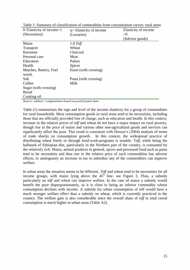
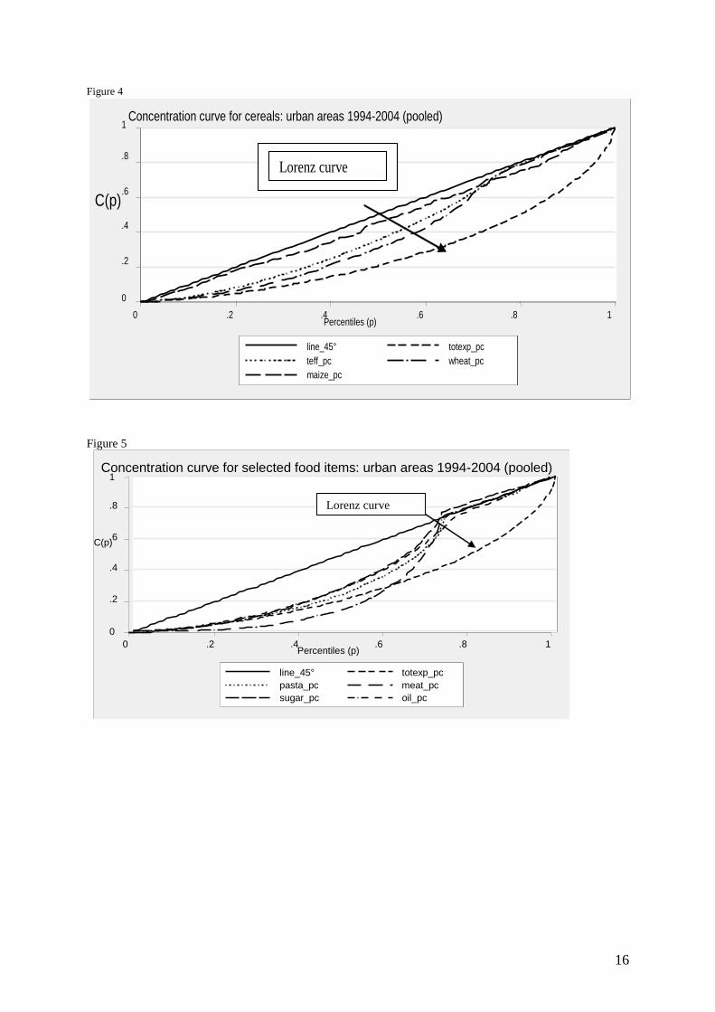
In urban areas the situation seems to be different. Teff and wheat tend to be necessities for all

income groups, with maize lying above the 450 line- see Figure 3. Thus, a subsidy

particularly on teff and wheat can improve welfare. In the case of maize a subsidy would

benefit the poor disproportionately, as it is close to being an inferior commodity whose

consumption declines with income. A subsidy for urban consumption of teff would have a

much stronger welfare effect than a subsidy on wheat, which is currently practiced in the

country. The welfare gain is also considerable since the overall share of teff in total cereal

consumption is much higher in urban areas (Table A2).

16

Figure 4

0

.2

.4

.6

.8

1

C(p)

0 .2 .4 .6 .8 1 Percentiles (p)

line_45° totexp_pc teff_pc wheat_pc maize_pc

Concentration curve for cereals: urban areas 1994-2004 (pooled)

Lorenz curve

Lorenz curve

Figure 5

0

.2

.4

.6

.8

1

C(p)

0 .2 .4 .6 .8 1 Percentiles (p)

line_45° totexp_pc pasta_pc meat_pc sugar_pc oil_pc

Concentration curve for selected food items: urban areas 1994-2004 (pooled)

Lorenz curve

17

Figure 6

0

.2

.4

.6

.8

1

C(p)

0 .2 .4 .6 .8 1 Percentiles (p)

line_45° totexp_pc kerosene_pc water_pc electricity_pc

Concentration curve for utilities: urban areas 1994-2004 (pooled)

Lorenz curve

As depicted in Figure 4 and 5, and also Table (2), urban consumption pattern exhibits

significant non-linearities in a large group of commodities, mainly at higher consumption

quintiles.

Table 2: Summary of commodity classification based on concentration curves: urban areas 0<Elasticity of income<1

(Necessities) > Elasticity of income (Luxuries) Elasticity of income <0

(Inferior goods) Wheat (super necessity after 7th

percentile)

Meat (cross Lorenz at 70th

percentile)

Teff Pasta (becomes necessity at higher

income)

Pulses (higher income)

Maize Cooking oil Shiro (higher income)

Sugar Clothing (crossing Lorenz curve at

60th

percentile)

Fruits(higher income)

Kerosene, Fuel Wood, Charcoal Transport (crossing Lorenz curve) Transport (higher income)

Water Fruits Water (at higher income level)

Electricity Drinks (crosses Lorenz curve at higher

income)

Electricity (higher income )

Salt Health expenditure (crosses Lorenz

curve)

Coffee, Tea (higher income)

Shiro

Pulses

Coffee, tea

Personal care

Education

Source: authors’ computations based on pooled panel data

In general, in addition to cereals, such items as sugar, kerosene, electricity, pulses, coffee, tea,

education expenses and personal care fall under the category of necessities in urban areas so

that an increase in the relative price of these commodities will have adverse effect more on

the poor population than the non-poor.

18

4.2. Inflation, inequality and consumption growth in Ethiopia

4.2.1. Illustration with the Linear Expenditure System

Results from the preceding section indicated that relative prices can have different

distributional impacts depending on whether a particular commodity is a necessity, luxury or

inferior commodity, and that it is important to distinguish between rural and urban areas. We

can extend this insight by linking the inequality of concentration curves with the overall

inequality of consumption expenditure. That is, it is possible to evaluate by how much overall

inequality as measured by the Gini coefficient changes due only to changes in relative prices

holding household income constant. We base our computations on the normative concept of

distribution of income that would maintain individual utility constant. To operationalize this,

we use one of the earliest and simplest expenditure systems used in the empirical literature,

the Linear Expenditure System, whose features have been sketched briefly in section 2. We

estimated the coefficients of Equation (2) using savings to identify all the parameters (see

Lluch, 1974 and Lluch and Powell, 1975).

The data used for this particular purpose is the urban Household Income and Consumption

Expenditure Survey collected by CSA in 1999/2000 since it has a wider coverage and is

nationally representative. We used single equation OLS to estimate first the parameters of

each group of consumption items, and used savings as a residual “consumption good” to

identify ii ip 1. Once the total subsistence expenditure is identified, then, we can use

equation (4) to compute the “true-cost of living index” as well as the magnitude of changes in

the Gini coefficient resulting from relative price changes. We used 9 commodity groupings,

including savings. The saving information includes only Iqub9 contributions and bank

deposits at the time of the survey.

9 Informal saving groups widely practiced in Ethiopia across all social groups.

19

Table 3: Robust Estimates of the parameters of the Extended Linear Expenditure System: urban areas,

1999/2000

Items iip

(Subsistence

consumption

expenditure, Birr)

i Per capita

consumption

expenditure (Birr)

Estimated

elasticity of

income

Cereals and Drinks 476

(6.68)**

0.43

(9.52)**

795

1.03

Household Items -43

(-2.97)**

0.08

(5.0)**

144

0.71

Clothing -33.0

(-2.12)**

0.12

(12.7)**

204

1.07

Transport -19

(-6.19)**

0.03

(2.05)**

30

1.02

Personal Care -34

(-3.0)**

0.04

(4.05)**

59

1.9

Recreation -29.9

(-5.8)**

.05

(6.0)**

96

1.3

Others 33.8

(0.71)

0.19

(5.04)**

512

1.0

Savings 0.0 0.06 51 …

** significant at 1%, terms in brackets are t-tratios.

Source: authors’ computations based on HICES data set

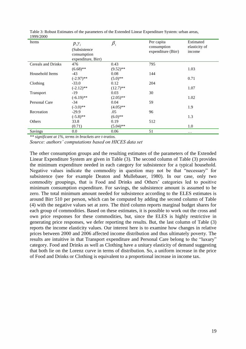
The other consumption groups and the resulting estimates of the parameters of the Extended

Linear Expenditure System are given in Table (3). The second column of Table (3) provides

the minimum expenditure needed in each category for subsistence for a typical household.

Negative values indicate the commodity in question may not be that “necessary” for

subsistence (see for example Deaton and Mullebauer, 1980). In our case, only two

commodity groupings, that is Food and Drinks and Others’ categories led to positive

minimum consumption expenditure. For savings, the subsistence amount is assumed to be

zero. The total minimum amount needed for subsistence according to the ELES estimates is

around Birr 510 per person, which can be computed by adding the second column of Table

(4) with the negative values set at zero. The third column reports marginal budget shares for

each group of commodities. Based on these estimates, it is possible to work out the cross and

own price responses for these commodities, but, since the ELES is highly restrictive in

generating price responses, we defer reporting the results. But, the last column of Table (3)

reports the income elasticity values. Our interest here is to examine how changes in relative

prices between 2000 and 2006 affected income distribution and thus ultimately poverty. The

results are intuitive in that Transport expenditure and Personal Care belong to the “luxury”

category. Food and Drinks as well as Clothing have a unitary elasticity of demand suggesting

that both lie on the Lorenz curve in terms of distribution. So, a uniform increase in the price

of Food and Drinks or Clothing is equivalent to a proportional increase in income tax.

20

Table 4: Welfare implications of relative price changes based on parameters of ELES: urban Ethiopia

Year National price index

i

i i

it

p

p

9

0

True cost of living index Gini coefficient

2000 100 1.000 1.000 0.330

2001 100.8 1.004 1.005 0.340

2002 96 0.998 0.988 0.344

2003 110.5 1.099 1.101 0.340

2004 120 1.181 1.186 0.339

2005 128.2 1.344 1.327 0.344

2006 143.9 1.606 1.561 0.350

Source: authors’ computations based on HICES data.

Table (4) reports measures of changes in the True Cost of Living Index10 as well as

simulated changes in the Gini coefficient due to inflationary processes. The second column of

Table (5) is the general price index obtained from the CSA. The third column provides the

weights in the changes in the relative index that is needed to estimate equation (4). The fourth

column provides the change in the True Cost of Living that takes fully into account

consumption behaviour. The last column is the Gini coefficient corresponding to each

period’s price regime with the assumption that nominal income remained constant. Important

points to note from this result are that first the True Cost of Living Index exceeds the general

price index by about 12% between 2000 and 2006. This means that the degree of welfare loss

due to inflation is much higher than implied by the general price index: that is households on

the average would need an additional 12% increase in expenditure to remain as well off as

they were in 2000, apart from adjustments they would need to make for the rise in the general

price index. Secondly, income distribution would worsen by about 2-percentage point

between 2000 and 2006 due only to inflationary processes. In effect, this means that inflation

tends to erode more the welfare base of the poor than the non-poor in urban areas. If the trend

of rising income inequality reported during the last decade (1994-2004) has prevailed in the

last two years also in urban areas (see (Bigsten and Shimeles, 2007), then, one would expect

a further worsening of poverty due to the inflationary process and changes in real prices. The

adverse effect of changes in prices on the poor implied here did not take into account the

possible offsetting increase in real per-capita income during the period. Still, the current

change in overall prices in urban areas tends to affect adversely more the poor than the non-

poor population.

10

The True Cost of Living Index is based on the total expenditure that a consumer needs to maintain the same

level of utility between two price regimes.

21

4.2.2. Consumption growth and price shocks

The above framework has a limitation in capturing welfare changes since it abstracts from the

simultaneous changes in relative wages, and in the rural context, incomes in the wake of

relative price changes. Thus, we may not be able to get the full impact of changes in prices on

household welfare. An economy wide model might be of help, but its data requirements and

the structure it imposes on the behaviour of economic agents, markets and institutions makes

it less attractive in the Ethiopian context. Availability of panel data at the household level

provides a rare opportunity to examine the price responses of consumption as in Dercon

(2004). This is a dynamic model where consumption growth for each household is allowed to

respond to price shocks after controlling for the effects of changes in other key determinants

of consumption. The model specified is:

itisit

s

sikt

k

kitiitit uSKPCC 1 (11)

Where itC is consumption expenditure by the ith

household in period t, itP is relative price

(in this case the terms of trade for agriculture), iktK represents household ith

’s k endowment

(land, education, oxen, etc..) and sitS captures other covariate or idiosyncratic shocks, such as

drought, illness, etc. Equation (11) provides a convenient framework to quantify the effect of

relative price shocks on the consumption growth of a typical household after controlling for

the contribution of other determinants of income. We estimate (11) by a linear transformation

through first-differencing (to identify ui) for households in rural and urban areas covering the

period 1994-2004 to decompose the change in consumption into components of shocks and

changes in human and physical capital.

Nearly all households in our sample in rural areas are farmers so that a rise in food prices,

particularly cereals, should be good for them as producers, but, bad as net buyers from

markets. For net sellers, the benefit is both from the real income side (better revenue from

crop sales) and improved utility from consumption of a commodity whose market price is

rising fast. The common method of identifying net-buyers and net-sellers is to take the

difference between reported crop sales and total crop output. Households with a net output

position are net-sellers. For such households, a rise in the price of cereals or grain brings

welfare gain through two channels, increase in household income as producers as well as

increase in utility as consumers depending on their preference for cereals. For net buyers, the

net welfare effect could be positive or negative, again depending on the strength of demand

responses to changes in income and prices. Thus, the welfare impact on rural households of

rising food prices is an empirical question. In Ethiopia, average income level is so low that

very few households have a surplus in their monthly household budget (Figure 7) putting a

majority vulnerable to price shocks.

22

Figure 7: household level budget deficit in rural areas: mean 1994-2004

Source: authors’ computations based on panel data

In a majority of cases, farmers in Ethiopia engage in the grain market in a complex way.

Most produce high value crops (such as teff) for the market to buy cheaper ones for

consumption, such as maize or barley. In other times, there is a tendency of switching to

export or cash crops (mainly chat) in response to relative price changes. Thus, the criterion

used to identify net sellers and buyers misses a very important dynamics in the choice of

crops for production and consumption. To partially address this, we instead use size of land-

holding as a potential indicator of net-crop position. A cursory look at the response of real

consumption growth to price shocks could be seen in Figure 8 for different household

groupings: land-rich, land-poor and the average household. The non-parametric estimate

suggests that more or less land-rich households tend to experience real growth in

consumption following rising food prices (weighted average prices of four types of cereals-

teff, wheat, maize and barley), while for the poorest consumption seems to have deteriorated

significantly.

-200

0

200

400

600

800

Hou

seho

ld b

udge

t def

icit

(per

mon

th p

er p

erso

n)

0 20 40 60 80 100Income percentile

23

Figure 8: real consumption growth and relative price changes by wealth status in rural

Ethiopia

Such divergent outcomes beg further investigation. The order of magnitude involved can be

obtained by estimating equation (11) for each category of households. We allow for the

persistence of shocks so that we estimate a dynamic consumption model not only as a

function of growth of endowments and shocks, we also include lagged consumption changes

as additional explanatory variable.

-1

-.5

0

.5

1

Gro

wth

in

re

al co

nsu

mp

tio

n p

er

ad

ult e

qu

iva

len

t

-.5 0 .5Rate of change in the price of cereals

Average poorest richest

24

Table (5) reports estimate of the parameters of equation (11) using Generalized Method of

Moments to deal with issues of endogenity as a result of the lagged consumption on the right

hand side of equation 11 (see for example Bond, 2002). We can infer from Table 5 that for

the average or typical farm household, rise in the price of cereals could lead to deterioration

in the rate of growth of consumption expenditure. A 1% increase in the rate of growth of

price of cereals could dampen the rate of growth of consumption by nearly 0.9%. On the

other hand, a rise in the rate of growth in the agricultural terms of trade leads to growth

acceleration in consumption.

Table 5:Real consumption growth and its determinants in rural Ethiopia: 1994-2004 Coef. z-values

Rate of growth in real per capita consumption(t-1) 0.058241 1.54

Rate of growth in agricultural terms of trade(t-1) 0.296366 8.59

Rate of growth in the price of cereals (t-1). -0.94347 -4.21

Rate of growth in crop sale(t-1) 0.056706 2.32

Rate of growth in hhsize(t-1) -0.76862 -8.86

Rate of growth in oxen ownership (t-1) 0.126832 5.36

Rate of growth in land size(t-1) 0.029682 1.13

1997 dummy 0.017889 0.37

2004 dummy -0.27786 -3.09

Village3*terms of trade -1.03093 -2.8

Village4*terms of trade 0.031806 0.19






_cons 0.074466 1.89

Sargan’s overidentification test 0.2806

Second order autocorrelation of eror terms

**significant at 1% level of significance

2.0 Source: authors’ computations based on the panel data

25

For the land-rich households, rising prices tend to contribute significantly to consumption

growth (Table 6). Both rise in real and nominal prices of agricultural prices contribute to

consumption growth for the land rich households suggesting that relatively wealthy farmers

could benefit from price reforms that favor the agricultural sector.

Table 6: Real consumption growth and its determinants in rural Ethiopia for land rich

households: 1994-2004 Rate of growth in real per capita consumption(t-1) 0.02413 0.45


Rate of growth in the price of cereals (t-1) 1.251573 2.22

Rate of growth in interaction terms b/n cropsales and cereal prices(t-1) -0.05496 -0.9




Rate of growth in land size(t-1) 0.019055 0.32

1997 dummy 0.164506 1.32

2004 dummy 0.478569 2.63

village4*tor -0.40467 -1.01

village5*tor -0.34491 -0.59

village6*tor -1.20123 -2.34

village7*tor -0.62834 -1.09

village 8* tor 0.817733 1.04

village9*tor -0.71678 -1.46

village 10*tor -2.02922 -1.8

_constant -0.07815 -1.09



The picture for land-poor households is rather bleak. They do not benefit from real price

increases and actually lose significantly from increase in the rate of price of cereals. A 1%

rise in the rate of growth of cereal prices could lead to 1.34% decline in real consumption

growth. To keep per capita consumption levels unchanged, poor farm households need much

innovation to do to raise farm productivity and identify other sources of income, such as non-

farm activities or employment with other farmers.

26

Table 7: Real consumption growth and its determinants in rural Ethiopia for land poor

households: 1994-2004 Rate of growth in real per capita consumption(t-1) 0.027867 0.42


Rate of growth in the price of cereals (t-1) -1.34007 -1.97

Rate of growth in interaction terms b/n cropsales and cereal prices(t-1) -0.21141 -1.89




Rate of growth in land size(t-1) -0.04482 -0.9

dummy 1997 0.667 4.67

dummy 2004 0.234161 0.95

village2*tor 0.181343 0.87

village3*tor -1.04528 -1.46

village 5*tor 3.636928 0.94

village6*tor -0.93955 -2.66

village7*tor -0.32782 -0.63

village8*tor -1.38326 -1.89

village10*tor 2.126619 2.14

_cons | 0.286125 4.08



The situation is straight forward for households in urban areas. Rise in the relative price of

food would decrease consumption expenditure significantly (Figure 9). During the decade

under investigation, real consumption per adult equivalent declined on the average by

approximately 1% in urban areas, while the real price of food in comparison to non-food

items increased by about 1.8% per annum, leading to an approximately 2.9% decline in

consumption (Table 8). So, over the decade, close to 30% of the decline in real consumption

growth could be attributed to rising food prices. The trend since 2004 in the rise of food

prices against non-food items is phenomenal. It is thus possible to imagine the

impoverishment of households in urban areas.

27

Figure 9: Non-parametric estimate of effect of relative price on consumption growth in urban areas: 1994-2004

Table 8: GMM estimate of consumption growth in rural Ethiopia: 1994-2004

Dependent variable: consumption growth in current period Coefficient z-ratio

Growth in one period lagged consumption .2847435 3.49**

Growth in two period lagged consumption .1942577 3.44**

Change in agricultural terms of trade -1.657991 -5.47**

Change in household size -.9795375 -10.29**

Change in real household asset ownership .0873953 3.46**

Lagged period dummy -.1339127 -1.54

Constant .3152891 3.39

Sargan’s overidentification test (P-value) 0.2179

**significant at 1% level of significance

-.8

-.6

-.4

-.2

0.2

Gro

wth

in r

ea

l co

nsu

mptio

n e

xpe

nd

iture

-.4 -.2 0 .2 .4 .6Change in relative prices of agricultural goods (TOT)

28

4.3. Own and cross-price elasticities for selected commodities using AIDS model

As part of the exercise to evaluate the welfare implications of changes in relative prices, in

this section we report demand responses to changes in prices and income. Estimates of price

and income elasticities can be useful for multi-market model analysis to examine the effects

of price changes. Our estimates are based on the AIDS model, which has several attractive

features, compared to say LES, which we estimated to illustrate welfare impacts of inflation.

The AIDS model does not impose a structure on the type of utility function so long as it

meets certain general criterion. Also linear Engel curves are not imposed (see section 3 for

details of model specification and some estimation issues).

We report here four specifications of the AIDS model with and without controlling for a set

of socio-economic characteristics of the household such as demographic profile, region of

residence, education of the head, sex of the head and others to get a robust elasticity

estimates. In all cases, restrictions required by choice theory are imposed on the coefficients.

These are the additive restriction, which states that all coefficients of the price variables add

up to unity, that the sum of marginal budget shares should add up to zero and symmetry of

the price responses which is related mainly with the positive-definiteness of the second order

condition for maximum ( or the Slutsky matrix).

Table 9: Price and income elasticities for rural areas using cereals as total consumption expenditure: restricted

AIDS model with socio-economic control variables

Price of Teff Price Wheat Price of Maize Expenditure elasticity

Teff -1.2527 -0.1620 0.0263 1.3887

Wheat -0.0179 -2.0862 1.2939 0.8114

Maize 0.2133 0.8815 -1.8260 0.8065

3.0 Source: authors’ computations based on the panel data Table 10: Price and income elasticities for rural areas using total consumption expenditure: restricted AIDS

model with socio-economic control variables

Price of Teff Price Wheat Price of Maize Price of Others Expenditure

Teff -0.0205 -1.8442 -1.0267 1.0020 1.7559

Wheat -2.7876 -3.6329 2.3150 2.5566 1.5811

Maize -1.5341 2.5285 1.4834 -3.7070 1.1606

Others 0.5276 0.5920 -0.6005 -1.1659 0.6425


Table 11: Price and income elasticities for rural areas using Quadratic AIDS model


Teff -2.19037 -0.82538 -0.83390 -0.92011 1.81868

Wheat -0.82538 -3.07998 -0.14283 -0.93583 1.84114

Maize -1.09564 -0.21623 -1.13090 -1.25064 1.55124

Others -1.13672 -0.99679 -2.63932 -0.79126 0.57190


The system of equations underlying the AIDS model has a non-linear component due to the

specification of the general price given in equation (7). To simplify the complications

involved we use instead the Lasperyes price index given by equation (8) to approximate the

general price index (see also Molina, 1994). By thus re-specifying equation (7) as in (8), we

make a linear approximation to the AIDS model. To allow for the possibility of non-linearity

29

of the Engle function, we used the Quadratic AIDS model fully specified in equation (11).

The system of equations is estimated by 3Stage Least Square method with the above

restrictions imposed on the coefficients. In addition, to allow for inter-temporal and spatial

comparison, we used real prices instead of nominal prices. For this reason, we deflated each

price variable with a weighted price index using 1994 as a reference period, and Harsaw, one

of our rural sites as reference. Thus, all prices are adjusted for spatial as well as temporal

variations.

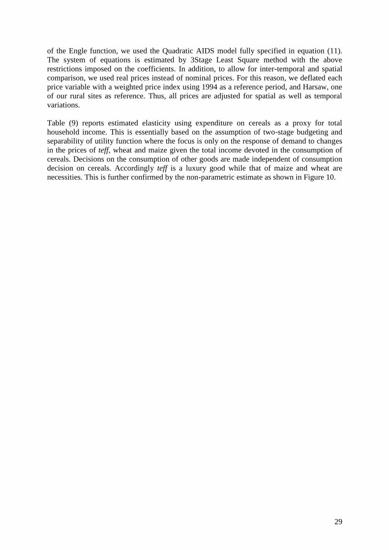
Table (9) reports estimated elasticity using expenditure on cereals as a proxy for total

household income. This is essentially based on the assumption of two-stage budgeting and

separability of utility function where the focus is only on the response of demand to changes

in the prices of teff, wheat and maize given the total income devoted in the consumption of

cereals. Decisions on the consumption of other goods are made independent of consumption

decision on cereals. Accordingly teff is a luxury good while that of maize and wheat are

necessities. This is further confirmed by the non-parametric estimate as shown in Figure 10.

30

Figure 10: Concentration curves for teff, wheat and maize using cereal expenditure as

reference

0

.2

.4

.6

.8

1

C(p)

0 .2 .4 .6 .8 1 Percentiles (p)

line_45° teff_exp

maize_exp wheat_exp cereal_exp

But, price responses tend to be stronger for the three types of cereals considered in our

analysis. Once we broaden our commodity groupings, the price and income response change

significantly. Table 10 for instance reports that teff, wheat, and maize become luxury items

once we allow choices for other goods also. Own price elasticities tend to remain stable

except for teff, which has declined markedly. Alternative commodity groupings are also

reported in Table A3 and A4 where we have taken a larger set of choices for households. In

this case, income elaticities for teff and wheat remained luxuries, and maize remained a

necessity. Allowing for the non-linearity of Engel function does not change the degree of

price or income responses of demand (Table 10). In fact, price and income responses tended

to be much stronger than the linearized version of the AIDs model in rural areas. The overall

trend regarding price responses is that the three typical cereals tend to be price elastic in

many specifications, with evidence of wheat being a close substitute for teff, especially in

cereal growing areas. This pattern is consistent across most of the alternative specifications,

and thus appears to be robust.

31

Table 12: Gross own and cross-price elasticities and expenditure elasticity of demand: narrow

classification(cereal growing rural areas)

Price of teff Price of wheat Price of maize Expenditure

Teff -1.43 0.83 -0.55 1.15

Wheat 0.28 -3.14 1.35 0.89

Maize 4.25 4.56 1.95 0.88


Table 13:Gross own and cross-price elasticities and expenditure elasticity of demand: narrow classification(Enset growing

areas)

Price of teff Price of wheat Price of maize Expenditure

Teff -1.06 -1.02 -2.80 1.79

Wheat 0.18 -0.28 0.04 0.64

Maize 2.00 1.93 2.17 0.99


Regarding urban areas teff and wheat tend to have an elasticity closer to unity when

allocation is restricted to cereals alone, suggesting some degree of being necessity and there

is strong own price response, which is understandable given the high degree of

substitutability indicated among these crops (Table 14). Maize tends to be an inferior

commodity (negative income elasticity or very low income elasticity) with relatively high

own-price responses. We also note that maize tends to be a good substitute for teff and wheat

in urban areas, perhaps explaining part of the high own-price elasticity (Table 15).

Table 14: Price and income elasticities for urban areas using cereals as total consumption expenditure: restricted linearized

AIDS model with socio-economic control variables

Price of Teff Price Wheat Price of Maize Expenditure

Teff -1.4645 0.1341 0.2176 1.1133

Wheat 1.1176 -1.1514 -0.7181 0.7479

Maize 4.3915 -1.8463 -2.5570 -0.1215


Table 15: Price and income elasticities for urban areas using Quadratic specification of the restricted AIDS Model

Price of Teff Price Wheat Price of Maize Expenditure

Teff -0.94465 -0.97383 0.64818 0.77179

Wheat -0.97383 -0.52042 -2.26954 0.82815

Maize -0.81174 -1.50334 -3.57145 0.36254


When we use broader commodity classifications with the Other group including total

consumption expenditure, less expenditure on teff, wheat and maize, the price and income

responses decline significantly. Teff, wheat and maize now become necessities for urban

households, which also remained unchanged as shown in Table A5 and Table A6. In

addition, allowing non-linearity in the Engel curve significantly changes the price and income

responses as shown in Table (16). Except for maize, the other cereals are now price and

income inelastic. This indicates the persistence of taste in affecting demand for teff and wheat

in urban areas and is also consistent with the non-parametric estimate discussed in the

preceding section.

32

Table 16: Price and income elasticities for urban areas using total consumption expenditure: restricted AIDS

model with socio-economic control variables


Teff -0.5961 -0.0535 0.1107 -1.0381 0.9405

Wheat -0.3266 -0.9996 -0.5682 0.9766 0.9186

Maize 2.1664 -1.3454 -2.7679 1.4143 0.5348

Others -0.2959 0.0854 0.0441 -0.8952 1.0618


33

5. Summary and conclusions

This study investigated the welfare implications of changes in relative prices in rural and

urban Ethiopia mainly based on a panel data of 3,000 households collected during 1994-

2004. This data was generated by the Department of Economics, Addis Ababa University, in

collaboration with University of Oxford and Gothenburg University. In addition, the

1999/2000 Household Income and Consumption Expenditure survey collected by the Central

Statistical Authority was also used to complement some of the analysis.

We found that changes in the prices of such consumption goods as teff, wheat and maize

could adversely affect the people at the higher income quintile in rural areas, while in urban

areas increased prices tend to affect those in the lower income quintile based on their

consumption patterns. Pair-wise comparisons of welfare dominance showed that most

consumption items tended to be necessities in rural areas and increases in the price of

transport, kerosene, coffee, cooking oil, and other consumption items would lead to the

worsening of welfare of poor households. This means that for example commodity specific

tax is not justified on welfare grounds. In urban areas, the choices for using specific

commodity taxes to finance subsidy on cereals are broader. Taxes on such wide range of

commodities, such as animal products (meat, milk, etc..), cooking oil, drinks, transport

services, utilities such as electricity, imported items to finance targeted subsidies on cereals

could potentially lead to higher welfare or less poverty. The current government program

intended to subsidize wheat through taxes on a wide range of commodities could be welfare

enhancing in urban areas.

Overall, the recent hike in relative prices was found to increase the true cost of living by an

additional 12% in urban areas, suggesting the severity of the welfare loss associated with

inflation. In addition, if unchecked, inflation in urban Ethiopia could worsen income

inequality significantly. It is estimated that between 2000 and 2006, the Gini coefficient

might have increased by 6.1% due to changes in relative prices, that were adverse to the

urban the poor. This result coupled with the recent trend of rising inequality in urban areas

(see for example Bigsten and Shimeles, 2006), suggests that gains in average per captia

growth can be eroded easily leading to growing impoverishment of households in urban

areas. The impact of rise in the real prices of cereals on the welfare of rural households is

more complex. To partially address this issue, we specified a dynamic model of consumption

growth, which is a function of changes in household endowments and price shocks. The

model was estimated for three distinct groups which potentially could address the net-

purchasing position of a household. These groups are: land-rich, land-poor and a typical farm

household. Our result imply that real growth in consumption is positive for land-rich

households while it remains negative for a typical farm household and deteriorates

significantly for the land-poor households. Certainly such significantly diverse outcome

would have a negative consequence on the pace of poverty reduction in rural areas.

Finally the study estimated a fully specified AIDS demand system for rural and urban areas

to generate effects of price and income changes on demand, particularly that of cereals. Using

pooled panel data, the estimates generally confirmed with what demand theory predicted.

Own price elasticities tended to vary significantly with different specifications in rural areas.

Overall, the evidence suggests that demand for teff, maize and wheat tends to be elastic, with

evidence of substitutability, especially between teff and wheat. In urban areas, all three types

of cereals tended to be necessities, and relatively price inelastic.

34

References

Ahmad ,E., and Stern, N., (1984), The Theory Of Indirect Tax Reform and Indian Indirect

Taxes, Journal Of Public Economics, 25, 259-298.

Atkinson, A.B., 1970, The Measurement of Inequality, Journal of Economic Theory, 2, 244-263.

Banks, J, Blundell, R., and A.Lewbel, (2004) “Endogenity in semi-parametric binary

response models”, Review of Economic Studies, 71: 655-679

Bigsten, A. and A. Shimeles (2006), “Poverty and Income Distribution in Ethiopia: 1990-

2004”, Department of Economics, University of Gothenburg, mimeo.

Bond, S. (2002), “Dynamic panel data models: A guide to micro data methods and practice”,

Cemmap Working Paper CW09/02, The Institute for Fiscal Studies. Department of

Economics

Cragg, M., 1991, Do we care; A study of Canada's Indirect Tax System’ Canadian Journal of

Economics, XXIV, No.1. Feb, 124-143

Haggablade, S and Younger. S. 2003. Indirect Tax Incidence in Madagascar: Updated

Estimates Using the Input-Output Table. Mimeo.

Deaton, A.S., 1981, Optimal Taxes and The Structure of Preferences, Econometrica, Vol.49,

1245-1260

Deaton, A. and J. Mullbeauer (1980): Economics and Consumer Behaviour, Cambridge

University Press. Cambridge

Dercon, S. (2005), “Economic Reform, Growth and the Poor: Evidence from Rural Ethiopia”,

Journal of Development Economics, 74(2):309-329

Kakwani, N., 1980 Income Inequality, and Poverty: Methods of Estimation and Policy

Applications, Oxford University Press

King., M., 1983, Welfare Analysis of Tax Reform, Journal of Public Economics, 21, 183-241

Molina, J.A., (1994), “Food demand in Spain: an application of almost ideal demand system”

Journal of Agricultural economics, 45, 202-258.

Myers, R and Bopape, L (2007), “Analysis of household demand for food in South Africa:

model selection, expenditure endogenity, and influence of socio-demographic effects”, paper

presented at the African Econometrics Society Annual Conference, Cape Town,

Roy, J., I.M., Chakravarty and R.G., Laha, 1959, A study of concentration Curves As

Description of consumption patterns, Studies In consumer Behavior, Calcutta: Indian

Statistical Institute

Tasciotti, L (2007), “Expenditure pattern in Italy:1875-1960: A complete quadratic demand

system estimation with demographic variables”, mimeo. University of Tor Vergata

Yitzhaki S. and Slmerod 1991, Welfare Dominance American Economic Review, Vol, No. 3,

480-495.

35

Table A1: Expenditure share by round and income quintile for rural areas of Ethiopia (1994-2004)… cont’d (next page)

Items 1994

2004

All Income Quintile Groups All Quintile Groups

Quint

1

Quint

2

Quint

3

Quint

4

Quint

5

Quint

1

Quint

2

Quint

3

Quint

4

Quint

5

Cereals 0.448 0.472 0.443 0.4159 0.4315 0.4926 0.4377 0.4399 0.3945 0.4256 0.4972 0.4989

Teff 0.1 0.08 0.082 0.0899 0.0857 0.1426 0.0856 0.0462 0.0577 0.0847 0.1342 0.149

Wheat 0.044 0.045 0.032 0.0436 0.0501 0.0667 0.0534 0.0276 0.0396 0.0654 0.0816 0.0698

Maize 0.096 0.08 0.094 0.1309 0.1105 0.1177 0.0773 0.0719 0.0861 0.0753 0.0863 0.0739

Sorghum 0.011 0.006 0.01 0.0106 0.016 0.0218 0.0219 0.0204 0.0313 0.0169 0.0273 0.0265

Millet 8E-04 0.001 1E-03 0 0.0005 0.001 0.0011 0 0.0015 0.0011 0.0011 0.0034

Animal Products 0.07 0.055 0.066 0.0852 0.0854 0.0915 0.0547 0.0289 0.0546 0.069 0.0517 0.0747

Pulses 0.066 0.069 0.07 0.0769 0.0672 0.0492 0.0903 0.0576 0.1023 0.1034 0.0942 0.0932

Drinks and

Stimulants

0.017 0.015 0.02 0.0177 0.0152 0.0196 0.0192 0.0107 0.023 0.0197 0.0248 0.0211

Enset 5E-04 0.001 5E-04 0.0004 0.0002 0 0.0011 0.0006 0.0015 0.0014 0.001 0.0008

Energy 0.025 0.026 0.03 0.0218 0.0188 0.0235 0.0336 0.0417 0.0386 0.0315 0.0268 0.0285

Personal Care 0.024 0.021 0.028 0.0261 0.0203 0.0259 0.03 0.0391 0.0331 0.0297 0.0261 0.0252

Clothes 0.106 0.102 0.095 0.1173 0.1208 0.1318 0.1094 0.0951 0.101 0.1214 0.1122 0.1315

Transport 0.015 0.011 0.009 0.0109 0.0185 0.0292 0.0166 0.0094 0.0124 0.0184 0.0207 0.0258

Health 0.019 0.013 0.017 0.0202 0.0257 0.0222 0.0206 0.0197 0.0232 0.0221 0.0203 0.0212

Education 0.005 0.003 0.006 0.0072 0.0062 0.0086 0.0111 0.0087 0.0114 0.013 0.0105 0.0138

Total Food 0.76 0.767 0.775 0.7627 0.7656 0.7348 0.6982 0.7188 0.7254 0.7264 0.7528 0.7234

Total Non-food 0.219 0.197 0.215 0.2305 0.2266 0.2652 0.2499 0.2443 0.2539 0.2597 0.2373 0.2707

36

Cont’d…. (Previous page) Table A1: Expenditure share by round and income quintile for rural areas of Ethiopia (1994-2004)

Items 1994-2004

All Quintile Groups

Quint 1 Quint 2 Quint 3 Quint 4 Quint 5

Cereals 0.4379 0.463 0.4316 0.4131 0.4627 0.4635

Teff 0.0933 0.0754 0.0686 0.0815 0.1026 0.1295

Wheat 0.047 0.0311 0.0381 0.0505 0.0637 0.0652

Maize 0.086 0.0785 0.099 0.1018 0.0935 0.08

Sorghum 0.017 0.0176 0.0205 0.0164 0.0176 0.0141

Millet 0.0018 0.0007 0.0016 0.0021 0.0028 0.0023

Animal Products 0.0506 0.033 0.0484 0.0545 0.0517 0.0674

Pulses 0.0783 0.0666 0.0806 0.0863 0.0843 0.0805

Drinks and stimulants 0.0192 0.0132 0.0188 0.0199 0.0225 0.0244

Enset 0.0006 0.0007 0.0009 0.0008 0.0005 0.0004

Energy 0.0239 0.0235 0.0282 0.0266 0.0227 0.0229

Personal Care 0.0281 0.0279 0.0286 0.03 0.0276 0.0289

Clothes 0.107 0.0915 0.0934 0.1095 0.1204 0.1268

Transport 0.0154 0.0083 0.01 0.0149 0.0192 0.0256

Health 0.0183 0.0132 0.0188 0.0216 0.0187 0.0204

Education 0.007 0.0047 0.0068 0.0077 0.0082 0.0092

Total Food 0.7385 0.7669 0.7624 0.7426 0.7311 0.7169

Total Nonfood 0.2278 0.1942 0.2173 0.2361 0.2408 0.2624

37

Table A2: Expenditure share by round and income quintile: Urban Areas Items 1994 2004 Pooled: 1994-2004

All All All Quintile Groups

Quint

1

Quint

2

Quint

3

Quint

4

Quint

5

Quint

1

Quint

2

Quint

3

Quint

4

Quint

5

Quint

1

Quint

2

Quint

3

Quint

4

Quint

5

Cereals 0.232 0.239 0.285 0.27 0.23 0.15 0.21 0.27 0.27 0.23 0.18 0.12 0.22 0.26 0.27 0.24 0.2 0.13

Teff 0.188 0.178 0.234 0.22 0.19 0.12 0.18 0.24 0.24 0.2 0.16 0.1 0.18 0.21 0.24 0.21 0.17 0.11

Wheat 0.029 0.034 0.029 0.04 0.03 0.02 0.02 0.02 0.02 0.02 0.02 0.02 0.02 0.02 0.02 0.03 0.02 0.02

Maize 0.015 0.026 0.021 0.01 0.01 0 0.01 0.02 0.01 0 0 0 0.01 0.02 0.01 0.01 0.01 0

Animal Products 0.075 0.015 0.035 0.07 0.11 0.14 0.08 0.01 0.03 0.06 0.11 0.15 0.08 0.01 0.03 0.06 0.11 0.15

Pulses 0.055 0.077 0.062 0.06 0.04 0.04 0.05 0.07 0.06 0.05 0.05 0.04 0.05 0.07 0.06 0.05 0.05 0.04

Drinks and stimulants 0.068 0.068 0.068 0.06 0.07 0.07 0.07 0.07 0.05 0.06 0.07 0.08 0.07 0.07 0.06 0.06 0.07 0.07

Energy 0.053 0.072 0.061 0.05 0.05 0.03 0.07 0.08 0.08 0.07 0.06 0.05 0.06 0.08 0.08 0.06 0.06 0.04

Personal Care 0.021 0.026 0.018 0.02 0.02 0.03 0.02 0.03 0.03 0.02 0.02 0.02 0.02 0.03 0.02 0.02 0.02 0.02

Clothes 0.04 0.009 0.028 0.03 0.05 0.08 0.04 0.01 0.02 0.04 0.05 0.09 0.04 0.01 0.03 0.03 0.05 0.08

Transport 0.036 0.012 0.035 0.04 0.03 0.06 0.04 0.03 0.04 0.04 0.04 0.05 0.04 0.02 0.04 0.04 0.04 0.05

Health 0.017 0.012 0.013 0.02 0.02 0.02 0.02 0.01 0.02 0.02 0.02 0.03 0.02 0.01 0.01 0.02 0.02 0.03

Education 0.098 0.118 0.1 0.1 0.09 0.09 0.05 0.05 0.05 0.05 0.04 0.05 0.07 0.08 0.07 0.07 0.06 0.06

Total Food 0.687 0.69 0.704 0.72 0.7 0.63 0.71 0.72 0.72 0.72 0.73 0.68 0.7 0.71 0.71 0.72 0.72 0.66

Total Non-food 0.203 0.177 0.194 0.18 0.2 0.25 0.25 0.24 0.25 0.25 0.25 0.27 0.23 0.21 0.23 0.23 0.23 0.27

38

Table A3: Price and income elastcities for selected commodities in urban areas using AIDS model without controlling for socio-economic factors

Price of Teff

Price Wheat

Price of Maize

Price of Milk

Price of Meat

Price of Sugar

Price of Coffee

Price of Cooking-oil

Price of Salt

Price of Pulses

Expenditure

Teff -0.92 -0.04 0.08 -0.31 -0.04 0.10 -0.10 0.12 -0.14 0.21 1.03

Wheat -0.25 0.55 -0.17 0.23 0.17 -0.44 0.20 -1.14 0.34 -0.48 1.03

Maize 1.32 -0.37 -6.34 0.08 -0.80 0.63 3.32 1.40 1.28 -1.02 0.63

Milk -1.92 0.16 0.00 0.17 -0.02 0.36 -0.23 -0.07 0.07 -0.24 1.70

Meat -0.38 0.08 -0.25 -0.01 -1.03 0.26 -0.18 -0.06 0.05 -0.18 1.59

Sugar 0.57 -0.33 0.20 0.38 -0.07 -1.50 -0.15 -0.23 -0.11 -0.01 0.85

Coffee -0.22 0.14 0.84 -0.08 0.10 -0.10 -0.83 -0.32 0.04 -0.05 0.61

Cooking-oil 0.42 -0.59 0.30 0.01 0.12 -0.16 -0.32 -0.43 -0.02 -0.19 0.97

Salt -2.19 1.10 1.71 0.37 0.41 -0.36 0.27 -0.01 -0.62 -0.68 -0.05

Pulses 1.26 -0.38 -0.37 -0.15 0.06 0.01 -0.06 -0.26 -0.20 -0.31 0.59

Table A4: Price and income elastcities for selected commodities in urban areas using AIDS model after controlling for socio-economic factors

Items

Price of

Teff

Price of

Wheat

Price of

Maize

Price of

Milk

Price of

Meat

Price of

Sugar

Price of

Coffee

Price of

Cooking-oil

Price of

Salt

Price of

Pulses

Expenditure

Teff -0.50 0.04 0.07 -0.11 -0.01 -0.18 -0.11 -0.10 -0.01 -0.10 1.01

Wheat 0.28 -0.17 -0.71 0.88 0.09 -1.05 0.59 -0.57 0.13 -0.44 0.98

Maize 1.20 -1.62 -5.78 -2.25 -0.81 1.75 2.64 3.56 -0.17 1.27 0.57

Milk -0.89 0.72 -0.87 -0.04 -0.01 0.21 0.02 -0.76 -0.51 0.46 1.77

Meat -0.27 0.02 -0.25 0.00 -1.02 0.15 0.00 -0.58 -0.38 0.33 1.66

Sugar -0.83 -0.80 0.57 0.25 -0.20 -0.57 -0.56 1.14 0.62 -0.88 0.86

Coffee -0.26 0.37 0.67 0.09 0.09 -0.41 -0.72 -0.65 0.17 -0.03 0.61

Cooking-oil -0.31 -0.29 0.79 -0.40 0.23 0.77 -0.61 -0.58 -0.15 0.23 0.96

Salt 0.18 0.45 -0.21 -1.67 0.45 2.54 0.93 -0.78 -1.76 2.06 -0.07

Pulses -0.38 -0.34 0.46 0.52 -0.05 -0.94 -0.04 0.42 0.55 -1.39 0.58

39

Table A5: Price and income elastcities for selected commodities in rural areas using AIDS model without controlling for socio-economic factors

Price of

Teff

Price of

Wheat

Price of

Maize

Price of

Milk

Price of

Meat

Price of

Sugar

Price of

Coffee

Price of

Cookingoil

Price of

Salt

Price of

Pulses

Expenditure

Teff -2.53 0.50 0.85 -0.06 -0.02 0.13 -0.68 0.49 -0.10 -0.17 1.71

Wheat 0.86 -2.84 1.04 -0.21 0.17 -0.42 0.23 -0.27 -0.01 -0.23 1.49

Maize 0.87 0.61 -2.92 0.02 -0.20 0.43 0.29 0.03 -0.34 -0.07 1.24

Milk -0.26 -0.78 0.15 -1.45 -0.26 -0.24 -0.18 -0.31 1.13 0.84 1.10

Meat 0.12 0.59 -0.79 -0.16 -1.89 -0.14 -0.10 -0.18 0.83 0.63 0.42

Sugar 0.79 -1.08 2.25 -0.16 0.66 -1.88 0.73 -0.66 0.73 -0.26 0.72

Coffee -0.46 0.21 0.37 -0.01 0.15 0.14 -0.89 -0.02 0.08 -0.07 0.63

Cooking-

oil

2.30 -0.48 0.21 -0.16 0.05 -0.50 -0.18 -1.47 -0.55 -0.30 0.85

Salt 0.06 0.13 -0.46 0.37 -0.02 0.34 0.15 -0.08 -1.13 0.32 -0.03

Pulses -0.87 -0.66 -0.22 0.83 0.47 -0.37 -0.81 -0.47 0.77 0.40 0.56

Table A6: Price and income elastcities for selected commodities in rural areas using AIDS model after controlling for socio-economic factors

Price of

Teff

Price of

Wheat

Price of

Maize

Price of

Milk

Price of

Meat

Price of

Sugar

Price of

Coffee

Price of

Cookingoil

Price of

Salt

Price of

Pulses

Expenditure

Teff -2.30 0.32 0.85 -0.08 -0.05 0.19 -0.69 0.46 -0.13 -0.14 1.72

Wheat 0.58 -2.89 1.04 -0.13 0.24 -0.48 0.22 -0.28 0.05 -0.13 1.47

Maize 0.87 0.60 -2.80 -0.02 -0.25 0.46 0.24 -0.05 -0.31 -0.08 1.25

Milk -0.41 -0.48 -0.12 -1.22 -0.07 -0.45 -0.03 -0.25 0.90 0.79 1.06

Meat 0.00 0.77 -1.06 -0.03 -1.63 -0.28 0.00 -0.03 0.68 0.60 0.41

Sugar 1.06 -1.24 2.39 -0.31 0.69 -1.58 0.72 -0.85 0.70 -0.41 0.74

Coffee -0.47 0.20 0.34 0.01 0.12 0.14 -0.89 0.06 0.10 -0.08 0.62

Cookingoil 2.24 -0.33 0.08 -0.12 0.05 -0.65 -0.11 -1.40 -0.53 -0.28 0.81

Salt 0.01 0.20 -0.40 0.30 -0.05 0.32 0.19 -0.08 -1.11 0.28 0.01

Pulses -0.67 -0.26 -0.26 0.78 0.44 -0.58 -0.85 -0.43 0.63 0.24 0.52

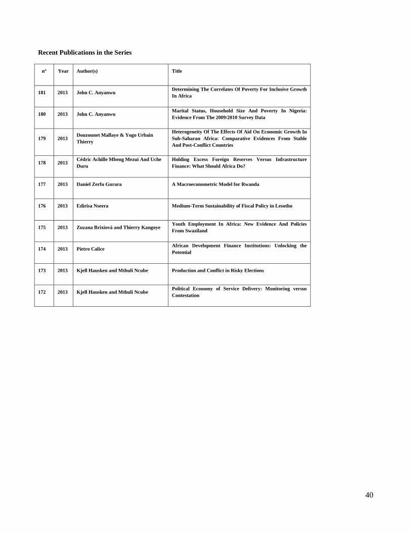
40

Recent Publications in the Series

nº Year Author(s) Title

181 2013 John C. Anyanwu Determining The Correlates Of Poverty For Inclusive Growth

In Africa

180 2013 John C. Anyanwu Marital Status, Household Size And Poverty In Nigeria:

Evidence From The 2009/2010 Survey Data

179 2013 Douzounet Mallaye & Yogo Urbain

Thierry

Heterogeneity Of The Effects Of Aid On Economic Growth In

Sub-Saharan Africa: Comparative Evidences From Stable

And Post-Conflict Countries

178 2013 Cédric Achille Mbeng Mezui And Uche

Duru

Holding Excess Foreign Reserves Versus Infrastructure

Finance: What Should Africa Do?

177 2013 Daniel Zerfu Gurara A Macroeconometric Model for Rwanda

176 2013 Edirisa Nseera Medium-Term Sustainability of Fiscal Policy in Lesotho

175 2013 Zuzana Brixiová and Thierry Kangoye Youth Employment In Africa: New Evidence And Policies

From Swaziland

174 2013 Pietro Calice African Development Finance Institutions: Unlocking the

Potential

173 2013 Kjell Hausken and Mthuli Ncube Production and Conflict in Risky Elections

172 2013 Kjell Hausken and Mthuli Ncube Political Economy of Service Delivery: Monitoring versus

Contestation

working paper 182 - rising food prices and household ... food prices and household welfare in...

Documents