1

Workhour Differences: The Labor/Leisure Choice

Chapter Overview

This paper continues the development of macroeconomic models based on

microeconomics. The models in these chapters that covered the issue of growth and

development were not truly modern in that they did not consider they took the savings

rate as exogenous. They were modern in that they included the profit maximizing

decision of firms and they studied the general equilibrium of the system. Still, they failed

to include the utility maximization problems of households.

This chapter moves us closer to a fully, micro founded model of the

macroeconomy. There are really two key decisions that consumers make in the context

of studying the macro economy. The first relates to labor supply worked, which is a

trade-off between work and leisure. The second relates to savings, which is a trade-off

between consumption today and in the future. This chapter considers the labor/leisure

decision of households, postponing the savings decision.

Despite this abstraction, the model we develop in this section is a useful device

for drawing scientific inferences, and it lays the foundation for much of what we shall do

in the remainder of the book. There are a number of questions that we can address with

it. One question is whether differences in tax rates on labor income across countries can

account for the observed differences in hours worked per person in these countries.

Consider the following Table taken from Edward C. Prescott’s (2004) article

titled, “Why do Americans work so much more than Europeans?” The table reports

average hours worked per week by the population aged 15-64 in the G-7 countries in both

2

the early 1970s and the mid-1990s. The Table shows that whereas Americans on average

worked shorter work weeks in the early period, they worked longer weeks in the later

period. In the early period, only the Canadians and Italians worked fewer hours per week

on average than Americans. However, in the later period, things are reversed; all

countries except the Japanese work shorter hours than Americans.

Hours per week per working age population ages 15-64

1970-74 1993-96

Germany 24.6 19.3

France 24.4 17.5

Italy 19.2 16.5

Canada 22.2 22.9

UK 25.9 22.8

Japan 29.8 27

USA 23.5 25.9

Source: Prescott 2004, Table 2.

Another question, and one you will be asked to answer, is what is the tax rate on

labor income that would maximize the government’s tax revenue? This question is one

that is particularly relevant to policy makers. Indeed, it was at the heart of the political

debate in the late 1970s, which brought Ronald Regan to the White House. One of the

promises that Ronald Regan made was to lower the marginal tax rate on people’s labor

income and increase the federal government’s tax revenues. The principal idea behind

this policy is known as the Laffer Curve, named after Arthur Laffer, (who purportedly

introduced the idea on a napkin at a cocktail party). The Laffer Curve shows the amount

3

of government revenues that are generated for tax rates between 0 and 100 percent. As

shown in Figure 1, government tax revenues are 0 when the tax rate is either 0 percent or

100 percent: if the tax rate is 0 percent, no taxes are collected; and if the tax rate is 100

percent, no rational individual will produce a thing knowing that the government is going

to confiscate all of his income. As the tax rate increases from 0 percent, tax revenues

must rise initially with the tax rate. Eventually, they must fall with the tax rate.

Consequently, there is a tax rate that maximizes the government’s tax revenues.

τ

Figure 1: The Laffer Curve

0 1.0 τ*

Tax

Revenues

4

Utility Maximization: Leisure and Consumption

In the utility maximization example studied in Chapter 2 there were two-goods. The

budget constraint was

Vpcc 21 (1)

Where p is the price of good 2 in units of good 1 and V is the consumer’s wealth also

measured in units of good 1. The utility maximizing condition sets the Marginal Rate of

Substitution in Consumption (MRSC) to the Marginal Rate of Substitution in Exchange,

which is

pcU

cU

1

2

/

/ (2)

Although it is natural to think of these two goods as say apples and oranges, we can think

of these two goods differently. For example, we can think of good 1 as apples and good 2

as leisure. Alternatively, we can think of good 1 as apples today and good 2 as apples

tomorrow. In this chapter, we will interpret the goods as apples and leisure. In the next

chapter, where we study the household savings decision, we will interpret the goods as

apples today and applies tomorrow. In terms of the mathematics, the interpretation we

give to the two goods is irrelevant in that the same utility maximization condition (2)

must hold.

To convince you that this is the case, let us examine the household’s problem

when utility is defined over consumption and leisure, c and l. An individual in any period

will only have a limited number of hours for which he can enjoy leisure. The other use of

his time is work. For now, let us fix these limited hours available to the person at 100 in

the period.

5

The indifference curves display the same shapes as before (i.e. downward sloping

and convex to the origin) and so the utility function is increasing in consumption and

increasing in leisure, and which is subject to the law of diminishing utility. The more

challenging issue is determining what the budget constraint for the household is in this

case? Let h denote the hours the household works, and the letter w to denote the wage

rate measured in units of the consumption good. (Instead of being paid in dollars, you are

paid in apples). If the household works, h, hours than he generates wh in income

measured in units of the consumption good. Then the amount of consumption the

household can afford is

whc (3)

If we use the fact that l+h=100, so that h=100-l, then the budget constraint is

wwlc 100 . (4)

This is just the same as before. The right hand side is not labor income, but your wealth-

the value of your time endowment, which you own.

The necessary conditions for household utility maximization are just as they were

before, namely,

cU

lUw

/

/ . (5)

2. General Equilibrium Analysis

From consumer theory, we obtain the household’s demand for goods and its supply of

inputs. From producer theory, we obtain the firm’s supply for goods and its demand for

6

inputs. The intersection of the supply and the demand for a final good or an input

determine its price and the quantity traded. General Equilibrium analysis simply requires

that all markets clear simultaneously.

To illustrate this, let us return to the model economy in which household utility is

defined over consumption and leisure. Namely, household utility is just

)log()log( dc , (6)

where the superscript d has been added to distinguish demand from supply. Without loss

of generality, we will assume that there is a single representative household in the

economy. The household takes prices as given.

On the producer side, we assume a production function that only uses labor as the

sole input, and for which the marginal product of labor is constant, rather than

decreasing. Thus, the Law of Diminishing Returns does not apply to the production side

of the economy. The production function does exhibit constant returns to scale.

Graphically, this production function is just a ray from the origin.

Mathematically, the production function is just linear in labor, namely,

ds Ahc (7)

where A is the Total Factor Productivity.

For this economy, we can define a competitive equilibrium.

Definition of Competitive Equilibrium

A competitive equilibrium for this economy is real wage rate, w a quantity of labor

supplied, hs , a quantity of labor demanded, h

d , production, c

s, and consumption, c

d, such

that

7

i. given the real wage rate, the consumer chooses cd and h

s to maximize utility

subject to his budget constraint.

ii. Given the real wage rate, firms choose cs and h

d to maximize profits

iii. The goods market clears; cs=c

d

iv. The labor market clears: hs=h

d.

We next solve out the competitive equilibrium for the household’s utility and the

firm’s production technology assumed above. We begin with the Household's problem.

The household utility is given by the following functional equations

)log()log( dc . (8)

The household’s budget constraint is

wwlc 100 . (9)

The utility maximization condition is

wh

c

l

c

cU

lUs

dd

100/

/ . (10)

We can use (10) to solve for cd. This is

)100( sd hw

c

. (11)

Next we substitute (11) into (9) using the fact that l=100-h. This gives us a single

equation in hs, for which we can solve for:

1

100sh . (12)

8

This is the household’s supply of labor. Notice, that the supply of labor is independent of

the price of labor, w, so that it is a vertical line. At first this may sound strange.

However, it is an implication of the choice of utility function.

To understand this, recall from microeconomic theory that when a price of a good

changes, there is both an income effect and a substitution effect. The substitution effect

always works to decrease the quantity demanded of a good as people will substitute away

from the good as the good's price increases. Here, if we think of an increase in the real

wage as an increase in the price of leisure, it is clear that the substitution effect will push

the consumer to work more. The income effect works in the opposite direction. Namely,

with a higher real wage, the household can work less hours and maintain the same

income. Since the household likes leisure, he shall want to take more leisure. With the

log utility, the two effects completely cancel each other out. This explains why the real

wage rate does not appear in the household's labor supply.

Profit Maximization

For the firm, its production function is just linear in labor, namely,

ds Ahc . (13)

The profit maximization condition described by (19) is just

A=w. (14)

Again, with this production function, the marginal product is constant so there is no law

of diminishing returns. Labor demand, therefore, is a horizontal line. If the wage rate

exceeds TFP, then the firm wants to hire zero workers. In the opposite case, the firm

would want to hire infinitely many as every worker would add to its profits by the

amount, A-w.

9

Graphically, the labor market is shown in the following diagram. The equilibrium

wage rate is just A, and the equilibrium quantity is just 100/(1+α).

The only issue that that remains in completing the characterization of the competitive

equilibrium is the quantity of consumption. This is easy, as once we have the equilibrium

quantity of hours, we can substitute this either into the production function or the

household’s demand function given by equation (11). In either case, we obtain that the

equilibrium amount of consumption/output

1

100 Ac . (15)

w

A

Labor Demand

Labor

Supply

Figure 8: Labor Market Equilibrium

1

100

h

10

This completes the characterization of the competitive equilibrium. Note that the

solution is in terms of the parameters of the model, and the endowment of the

household’s time. This will always be the case in solving for a competitive equilibrium,

namely, the equilibrium quantities and prices are expressed as functions of only the

model parameters and the endowments.

3. Government Policy

Having laid out the basic model and solved for the general equilibrium prices and

allocations, we now turn to the questions motivating this chapter. Why did Americans

tend to work less hours per week relative to other G-7 countries in the 1970s but more in

the 1990s. Relatedly, what is the tax rate on labor that maximizes government tax

receipts? For this reason, we reintroduce government into the static model used in the

previous section.

Government Budget Constraint

In general governments buy goods and services. They generate tax revenues from labor

income, as well as from other forms of income such as capital income. In many countries,

taxes on consumption are an important source of government revenues. They also make

payments to households. These are known as transfer payments. Now, a government

whose outlays are greater than its tax receipts can borrow. Of course, it will need to pay

off the interest and principle on its previous borrowings. Since the model is static, there

11

can not be any borrowing or lending. 1 Additionally, since our model does not have any

capital, there cannot be any capital income taxes in our static model.

Taxes and Transfers

For now, we shall consider a limited form of government policy, namely, where the

government only imposes a tax on the household’s labor income and then rebates all of

the tax receipts back to the household in a single check in the form of a lump-sum

payment. The key feature of the lump-sum payment is that the household views the

payment amount to be independent of any decision it makes.

If the government taxes the household’s labor income at a tax rate of τ, what this means

is that for each hour worked the household keeps (1-τ)w. Additionally, by assumption

the household has a second source of income, the lump-sum transfer by the government.

If ψ denotes the lump-sum transfer, (which could be negative in which case it would be a

lump-sum tax), then the budget constraint is just

whc )1( . (16)

Using the time use constraint for households, we can rewrite the budget constraint as,

wwlc )1(100)1( . (17)

As the total amount of tax revenue collected equals the amount of lump-sum transfers,

the government's budget constraint is

1 Governments can also print money if tax revenues are deficient. This has been a common method used

by many countries, particularly Latin American countries in the post war period. As there is no money in

our model, i.e., it is a real economy, we do not consider this possibility in this chapter.

12

hw . (18)

Now that we have introduced the government into the model, we shall want to

solve for the competitive equilibrium.

Competitive Equilibrium

There are still two markets in this economy: the labor market and the goods market. A

competitive equilibrium for this economy is still a real wage rate, w a quantity of labor

supplied, hs, a quantity of labor demanded, h

d, production, c

s, and consumption, c

d. In

addition, there is the government policy, given by the tax rate on labor income τ and the

lump-sum transfers, ψ. This price, allocations, and policy must satisfy the following

conditions:

i. Given the real wage rate, the tax rate and lump-sum transfers, the consumer

chooses cd and h

s to maximize his utility subject to its budget constraint.

ii. Given the real wage rate, firms choose cs and h

d to maximize profits

iii. The government’s budget is satisfied, namely hw

iv. The goods market clears; cs=c

d

v. The labor market clears: hs=h

d.

To solve for the competitive equilibrium we start with the household’s utility

maximization problem. Equating MRSC=MRSE implies

wl

c)1(

(19)

Next, we rewrite (19) using the time use constraint of the household so that we

MRSC=MRSE is expressed in terms of hours rather than leisure. This is

13

wh

c)1(

)100(

(20)

Next, we shall use the goods market clearing condition c=Ah, together with the profit

maximizing condition that w=A and substitute into (20). This gives

)1()100(

h

h (21)

From (21), we arrive at the equilibrium value for work hours

100))1((

1

h (22)

It is easy to show that h is a decreasing function of τ, so that a higher tax rate reduces

work hours in the economy.

What is the intuition for this result? Recall, our utility function is characterized

by a unit elasticity of substitution so that a 1% increase in the wage has no effect on work

hours. It is true that putting a tax on labor income in effect represents a change in the

relative price of leisure, and so in this sense the tax rate has no effect of the household’s

leisure choice. However, the lump sum transfer that is paid back to the households acts as

type of gift to the household, that makes the feel wealthier and hence makes them want to

buy more consumption and leisure. The following two figures represent the difference

between a change in relative prices (without the transfer), and the change in relative

prices with the transfer. As can be seen the transfer ψ allows the consumer to consume

consumption up to ψ even when the household does not work.

14

c

leisure

Figure 5.a: Choice of Leisure –No

transfer

1U

0U

15

Comparing Alternative Policies: Welfare Analysis:

For any tax rate, we can compute the competitive equilibrium. While we can easily show

how the prices and quantities are affected by tax policy, we ultimately want to know what

happens to households' welfare. As the tax rate changes, a household's consumption and

leisure will change. An interesting question is how will the household’s welfare differ

across alternative tax policies? To compare welfare across different policy regimes, we

will determine the factor that we must scale consumption by so that the utility of the

household in the equilibrium when the tax rate is set to some value, (say τ = .40) equals

the utility realized by the household in the case that the tax rate is at a lower value. This

gives the household’s welfare in terms consumption differences.

Consider as an example a policy experiment whereby the tax rate on labor income

would be raised from .40 to .60. Household welfare will be lower under the higher tax

c

leisure

Figure 5.b: Choice of Leisure –with

transfer

1U

0U

16

rate. Thus, we would like to know by how much we would have to increase the

consumer’s consumption so that his utility is equal to the utility that he realizes with the

lower tax rate of .40. Mathematically, we are interested in finding the value of the

scaling factor, 1+, such that

))60.0(100log())60.0()1log((

))40.0(100log())40.0(log(

hc

hc (23)

Therefore, (1+) is the factor that consumption must be scaled if there is a change in the

tax rate from 40% to 60% to leave people indifferent to the change. The welfare loss in

consumption equivalents is c .

In general, it is not possible to determine this compensation factor without

assigning parameters to the model. This is the goal of the calibration procedure. We now

illustrate the calibration procedure within the context of the static model with government

policy.

III. Calibration Application: Work Hour Differences

We next use the model with government taxes to understand the differences in work

hours per person of working age across G-7 countries by undertaking a calibration

exercise that is based on Prescott (2004). We proceed in detail by going through each of

the five steps. However, before doing so, it is useful to consider the issue in the context

of labor market outcomes.

One reasonable question to ask about the observation that Americans in the 1990s

worked more than their G-7 counterparts whereas the opposite was the case in the 1970,

is whether differences in unemployment rates across countries and across time are

important to understanding differences in work hours. Additionally, since work hour per

person are averages over the working age population there is also the question of whether

how much of these differences are the result of differences in participation rates.

17

A person is defined to be in the Labor Force (LF) if he is

either employed (E) or looking for employment, that latter of which

are defined as unemployed (U). Thus, LF=E+U. A country’s

unemployment rate (UR) is simply the number of unemployed

divided by its labor force, namely, UR=U/LF. A country’s

participation rate (PR) is equal to its labor force divided by its

population of people above 15 years of age. If P denotes the

working age population, then a country’s participation rate,

PR=LF/P.

Let h be the average hours worked per worker. Then the

hours, H, worked per person (above age 15) is

P

EhH (24)

Next, we shall use the fact that LF=E+U, PR = LF/P=(E+U)/P. and

UR=s U/LF to rewrite (24) as

)1( URhPRH (25)

Equation (25) thus allows us to decompose the average hours per

working age population into hours per worker, the participation rate,

and the employment rate, or 1 less the unemployment rate.

[Insert Figures 6-7]

Although unemployment rates and participation rates have

increased over the two sub-periods for most of the G-7 countries, it

is not the case that either changes in PR or ER account for change in

Employment, Unemployment and the Labor Force

Unemployment and Employment

Statistics are based on household survey

data taken on a monthly or quarterly

basis. Although each country’s surveys

are conducted by its own agency, the

same criteria are used to classify

households as being employed or

unemployed. (The source of each

country’s employment statistics can be

found here.) As stated on the OECD

webpage for Labour Statistics these

criteria are as follows:

Employment - Persons

in civilian employment

include all those employed

above a specified age who

during a specified brief

period, either one week or

one day, were in the

following categories: i) paid

employment; ii) employers

and self-employed; iii) unpaid

family workers; unpaid

family workers at work

should be considered as being

self-employed irrespective of

the number of hours worked

during the reference period.

For operational purposes, the

notion of some work may be

interpreted as work for at

least one hour. Total

employment is defined as the

sum of civilian employment

and members of the armed

forces.

Unemployment - The

unemployed comprise all

persons above a specified age,

who during the reference

period were: i) without

work, i.e. were not in paid

employment or self-

employment during the

reference period; ii) currently

available for work, i.e. were

available for paid

employment or self-

employment during the

reference period; iii) seeking

work, i.e. had taken specific

steps in a specified recent

period to seek paid

employment or self-

employment.

18

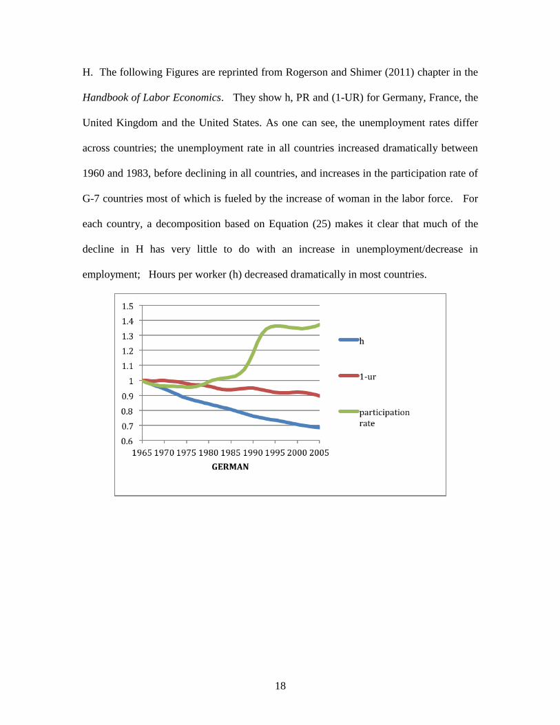
H. The following Figures are reprinted from Rogerson and Shimer (2011) chapter in the

Handbook of Labor Economics. They show h, PR and (1-UR) for Germany, France, the

United Kingdom and the United States. As one can see, the unemployment rates differ

across countries; the unemployment rate in all countries increased dramatically between

1960 and 1983, before declining in all countries, and increases in the participation rate of

G-7 countries most of which is fueled by the increase of woman in the labor force. For

each country, a decomposition based on Equation (25) makes it clear that much of the

decline in H has very little to do with an increase in unemployment/decrease in

employment; Hours per worker (h) decreased dramatically in most countries.

19

20

Data Resource: The annual hours, 1-unemployment rate and participation rate is relative

to 1965 level. They are handled by HP filter. Data for annual hours per worker in

employment are from the Groningen Growth and Development Center(GGDC), Total

Economic Database. The participation rate is calculated by using data active population

from OECD StatExracts. The activte population divided by the total populatioin. The

active population is the sum of unemploymed population and employed population. The

total population data is from GGDC. The active population data is missing for UK from

1992-1999, so these data is replaced by using participation rate from U.S Bureau of

Labor Statistics: the International Comparisons of Annual Labor Force Statistics,1970-

2012.

To make the point that unemployment is not an important factor in understanding

work hour differences of the working age population, Rogerson and Shimer compute H

for each country in Equation (25) fixing (1-UR) at the US rate and using each country’s

own h and PR. What they find is the difference in hours per person obtained by using the

US employment rate is very similar to the actual hours per person.

21

These findings suggest that the issue of unemployment is not important for

accounting for work hour differences. This is important as our model does not consider

the issue of unemployment. Our model assumes perfectly competitive markets with a

wage rate equal to its marginal product. It is classical in that given the equilibrium wage,

everyone is happy about the amount of time they work or do not work. The study of

unemployment, specifically of differences in unemployment rates across countries, will

require a different type of model.

Calibration Steps

Recall there are 5 steps: pose a question; choose a model; define consistent measures;

assign parameters, and comparison of model predictions with data. We now go through

each of the 5 steps.

a. Pose a Question.

We can use the model in this section to answer a number of relevant questions. One

question is “What is the tax rate that maximizes the government’s tax receipts?” Another

related question is “What would be the effect on household welfare if Europe adopted the

U.S. tax rate on labor income equal to .40 instead of its current tax rate of .60?

b. Choice of model

Here the issues are what things to put in the model, and what functional forms should

utility and production take. Obviously, the question one poses has a lot to do with what

goes in the model. As we are interested in how tax rates affect work hours, it is critical

22

that we allow for the household to trade off between leisure and work. Thus, it is critical

that we define utility over both consumption and leisure.

As for the functional forms, we want to use both theory and data to guide us in

their selection. In solving for the competitive equilibrium, we used a utility function of

the form log (c) + α log (l). This was not by accident. Recall, that in the model without

taxes we showed that the labor supply is unaffected by changes in the real wage. That is

because with the log utility function the substitution effect exactly offsets the income

effect.

This utility function is consistent with the long-run record of the United States.

The real wage in the United States has grown at roughly 2 percent per year over the 20th

century. Despite this increase, there has been no secular change in the hours worked by

households, at least in the post World War II period. What this suggests is that the entire

increase in the real wage has gone to pay for more consumption by households.

Alternatively, a one percentage increase in the real wage rate has been associated with a

one percent increase in consumption. This is just saying that the elasticity of substitution

between consumption and leisure goods is unity. This effectively limits the functional

forms for household utility.

The production function was chosen so that there are constant returns to scale.

With constant returns to scale, profits of firms are zero provided each factor is paid its

marginal product. Zero profits is consistent with perfect competition. Additionally, with

constant returns to scale, the size of firms is unimportant in the economy. In the U.S.

economy, some firms in an industry are large while others are small. This is consistent

with the constant returns to scale technology.

23

If you have been paying attention, the question you should now ask yourself is

why would a change in the tax rate on labor income change the amount of time an

individual works? If the log utility implies that the substitution and income effects cancel

each other out, how can it be the case that the tax rate affects work hours, as the tax rate

effectively determines the real wage the consumer takes home? As you shall see, a higher

marginal tax rate on labor income will decrease the equilibrium work hours. The

substitution and income effects still cancel each other out. So what is going on here? This

is a good question, and one that you are assigned to answer on your own. A helpful hint:

What happens to the tax revenues that are collected by the government?

c. Defining Consistent Measures

The model is truly abstract. For instance, there are no investment expenditures or

government expenditures. All output is consumption. Additionally, there is no capital,

so all income is paid to labor. Normally, we would have to rearrange the National

Income and Product accounts around the categories of the model. For instance, we would

need to add all investment and government expenditures in the NIPA to consumption.

While we could do this, it is really not essential for completing steps 4 or 5 of the

calibration exercise. This is because these steps only involve the data on hours worked,

which are directly comparable between the model and the data.

d. Assignment of parameters

The next step is to assign parameters to the model. There are three parameters: the tax

rate, τ, preference parameter, α and the TFP parameter, A. The value of A only

24

determines the choice of units for measuring output and prices. For this reason, we can

proceed to normalize its value to 1. In effect, it doesn't matter if we measure the output of

the dairy industry in gallons, half gallons, or pints. In the case we measure it in pints,

output will be smaller, and this will be reflected by a smaller value of A. The tax rate is

chosen to the value in the U.S. economy, which is equal to .40. This leaves the leisure

parameter, α. This can be pinned down by using the observations for h=25 in the United

States, and the household utility maximization condition

)100)(1( sd hw

c

,

together with the result that in equilibrium c = Ah . This is left for you to do as an

exercise.

Notice that if we started with this value of α and proceeded to solve for the

equilibrium with the tax rate equal to .40 and A= 1.0, we would find that in equilibrium

h=25. In effect, Step 4 of the calibration exercise is akin to an inverse problem to

finding the equilibrium. We know the equilibrium property, namely h=.25. What we

want to find is the value of α that gives us this equilibrium result.

e. Test of the Theory

The question we posed is a policy related question. If it were a test or development of

theory related question, such as do tax rate differences account for the differences in

work hours observed between the rich industrialized countries, we would want to

compare the predictions of the model for work hours as we vary the tax rate to market

hours worked in various countries with their tax rate on labor income. This is what

Prescott (2004) does in trying to see if differences in tax rates between OECD countries

25

can account for the fact that in the 1970s Europeans worked more than Americans on a

per person basis while in the 1990s the opposite was true.

For the policy evaluation at hand, we simply compute the equilibrium for

alternative tax rates and determine the welfare differences between policies. What we

really want to do is to determine what side of the Laffer curve the United States is on. If

the current tax rate of .40 is to the left of the maximum tax revenues, than increasing the

tax rate is a good idea from the standpoint of increasing government tax revenues. If the

opposite holds, then increasing the tax rate will actually lower the government's tax

revenues. This is also left as an exercise for you to do.

IV. The Uses of Tax Revenue: The Scandinavian Outliers

Richard Rogerson in a 2007 paper title Taxation and Work Hours: Is Scandanavia an

Outlier? published in Economic Theory pointed out that the Scandinavian countries in

general have higher marginal tax rates than Western Europe, yet work more hours per

person. Does this mean that Prescott (2004) was wrong in arguing that differences in tax

rates can account for most of the observed differences in work hours among OECD

countries? Rogerson's answer is that Prescott’s findings are not necessarily wrong,

because households work hour responses to taxes will depend critically on the how the

government spends the tax revenues.

Rogerson considers four types of government programs, including the lump-sum

transfer program studied by Prescott and presented in Section 2. We now present each in

turn.

26

Program 1: Useful government transfers

This is just the case studied in Section 3 of this chapter. The key feature of this program

is the lump-sum payment of tax revenues back to the household. Although we model this

as a rebate check from the government, the key aspect of this policy is that the

government revenue provides something that the consumer values. This can be in the

form of added purchasing power to consumers, (outright income transfers), goods that the

government buys and transfers to consumers (education, judicial, health), or employs

workers to produce output transferring the output to consumers.

In the case of useful government transfers, the household’s budget constraint is

whc )1(

and the Government Budget Constraint is

wh0

Examples: Government revenue is used to provide something that the consumer values.

This can be in the form of added purchasing power to consumers, (outright income

transfers), goods that the government buys and transfers to consumers (education,

judicial, health), or employs workers to produce output transferring the output to

consumers.

Solving for the Equilibrium: The utility maximization condition is:

wh

c)1(

)100(

In equilibrium c=wh, and w=A. Hence

27

)1()100(

h

h

This yields the familiar solution given by Equation (22)

100))1((

1

h

Program 2: Useless government expenditures

In this case the government uses the tax revenues to buy output. The key property of this

program is that the use of the government revenue yields no utility to consumers and does

not enhance the productivity of firms. Here the best example is probably military

services. Much of employment in the public sector could be classified as useful

government expenditures.

The household’s budget constraint is

whc )1(

and the Government Budget Constraint is

whg

FONCs:

wh

c)1(

)100(

In equilibrium, since whg , whc )1( . Hence

)1()100(

)1(

h

h

It is immediate apparent that taxes rates have no effect on the equilibrium work hours in

the case of useless government expenditures. We have

28

1

100h

Program 3: Consumption subsidy.

Another use of tax revenues is to subsidize the consumption purchases of households.

Here the key is that government subsidizes consumption at the margin. Examples that

Rogerson lists are subsidized child care or elderly care. In Sweden, the child care

transfers are actually made conditional on both parents working.

For this policy, for every $1 spent by the consumer on goods and services, the

subsidy would rebate back s cents. In the case of the consumption subsidy, the

household’s budget constraint is

whcs )1()1(

And the Government Budget Constraint is

whsc

FONCS

wh

cs)1(

)100(

)1(

In equilibrium sc=τwh, and w=A and c=h, hence

Ah

hA

h

hhA)1(

)100(

)1(

)100(

)(

.

Thus, equilibrium work hours are independent of taxes and are just

1

100h

Program 4: Subsidy to leisure;

29

The final type of use of tax revenues is a transfer that depends on how much leisure the

consumer enjoys. An example of this type of transfer is unemployment compensation.

In particular, for each unit of leisure enjoyed by the household, he or she enjoys a transfer

of b units of the good. Note that this is not a lump-sum transfer as it depends on leisure,

or how little you enjoy. The household’s budget constraint is

blwhc )1(

The Government Budget Constraint is

blwh

FONCS

bwh

c

)1(

)100(

In equilibrium c=Ah, and w=A and )100( hbwh , hence

bAh

hA

)1(

)100(

h

A

h

AhA

h

hA

1001

100)1(

)100(

hh )1(100

So that

1

)1(100h

Findings: Rogerson points to key differences in the use of government tax revenues

between Scandinavia and Continental Europe as a way of reconciling Prescott’s

conclusions with the Scandinavian experiences. For example, he points out that

Government spending on family services in Scandinavia is 8% of GDP whereas it is 2%

30

in continental Europe 2%; Additionally, he points out that government employment to

total employment is 15% in the US, 18% in Continental Europe, and 28% in

Scandinavia. If these expenditures are wasteful, then according to Case 2 above they do

not change work hours. Rogerson argues that half of these expenditures in Scandinavia

are wasteful. Rogerson concludes that these differences gets you most of the difference

between Continental Europe and Scandinavia.

V. Conclusions

In this chapter we introduced the labor/leisure decision and government policy,

and used the model to examine how much of the differences in work hours observed

across G-7 countries in the 1970s and the 1990s could be accounted for by differences in

tax rates. The conclusion of the calibration exercise is that tax rate differences across

countries and across time can account for most of the differences in hours worked per

week per person aged 15 to 65.

Quantitative Exercises:

1. Calibrate model under program x to US and then change the tax rates.

2. More interesting, calibrate the model with all four programs in the US and then change

the tax rates.

31