word embeddings: history & behind the...
TRANSCRIPT

Word Embeddings: History & Behind the Scene
Alfan F. WicaksonoInformation Retrieval Lab.
Faculty of Computer ScienceUniversitas Indonesia

References
• Bengio, Y., Ducharme, R., Vincent, P., & Janvin, C.(2003). A Neural Probabilistic Language Model. TheJournal of Machine Learning Research, 3, 1137–1155.
• Mikolov, T., Corrado, G., Chen, K., & Dean, J. (2013).Efficient Estimation of Word Representations in VectorSpace. Proceedings of the International Conference onLearning Representations (ICLR 2013), 1–12
• Mikolov, T., Chen, K., Corrado, G., & Dean, J. (2013).Distributed Representations of Words and Phrases andtheir Compositionality. NIPS, 1–9.
• Morin, F., & Bengio, Y. (2005). Hierarchical ProbabilisticNeural Network Language Model. Aistats, 5.

References
Good weblogs for high-level understanding:
• http://sebastianruder.com/word-embeddings-1/
• Sebastian Ruder. On word embeddings - Part 2:Approximating the Softmax. http://sebastianruder.com/word-embeddings-softmax
• https://www.tensorflow.org/tutorials/word2vec
• https://www.gavagai.se/blog/2015/09/30/a-brief-history-of-word-embeddings/
Some slides were also borrowed from From Dan Jurafsky’scourse slide: Word Meaning and Similarity. Stanford University.

Terminology
• The term “Word Embedding” came from deeplearning community
• For computational linguistic community, they prefer“Distributional Semantic Model”
• Other terms:– Distributed Representation
– Semantic Vector Space
– Word Space
https://www.gavagai.se/blog/2015/09/30/a-brief-history-of-word-embeddings/

Before we learn Word Embeddings...

Semantic Similarity
• Word Similarity– Near-synonyms
– “boat” and “ship”, “car” and “bicycle”
• Word Relatedness– Can be related any way
– Similar: “boat” and “ship”
– Topical Similarity:• “boat” and “water”
• “car” and “gasoline”

Why Word Similarity?
• Document Classification
• Document Clustering
• Language Modeling
• Information Retrieval
• ...

How to compute word similarity?
• Thesaurus-based Approach– Using lexical resource, such as WordNet, to compute
similarity between words
– for example, two terms are similar if their glossescontain similar words
– For example, two terms are similar if they are neareach other in the thesaurus hierarchy
• Distributional-based Approach– Do words have similar distributional contexts?

Thesaurus-based Approach
• Path-based similarity
• Two terms are similar if they are near each other inthe thesaurus hierarchy
Hypernym Graph

Thesaurus-based Approach
Other Approach:
• Resnik. 1995, using information content toevaluate semantic similarity in a taxonomy.IJCAI.
• Dekang Lin. 1998. An information-theoreticdefinition of similarity. ICML.
• Lesk Algorithm

Thesaurus-based Approach
Problems...
• We don’t have a thesaurus for every language
• For Indonesian, our WordNet is not complete
– Many words are missing
– Connections between senses are missing
– ...

Distributional-based Approach
• Based on the idea that contextual information aloneconstitutes a viable representation of linguistic items.
• As opposed to formal lingustics and the Chomskytradition.
• Zellig Haris (1954): “...if A and B have almostidentical environments, we say that they aresynonyms...”
Word Embeddings are based on this idea!

Distributional-based Approach
A bottle of is on the tableEverybody likes tesgüinoTesgüino makes you drunkWe make tesgüino out of corn
• From context words humans can guess tesgüino means• an alcoholic beverage Like beer
• Intuition for algorithm:• Two words are similar if they have similar word contexts
From Dan Jurafsky’s course slide: Word Meaning and Similarity
tesgüino
Distributional-based Approach
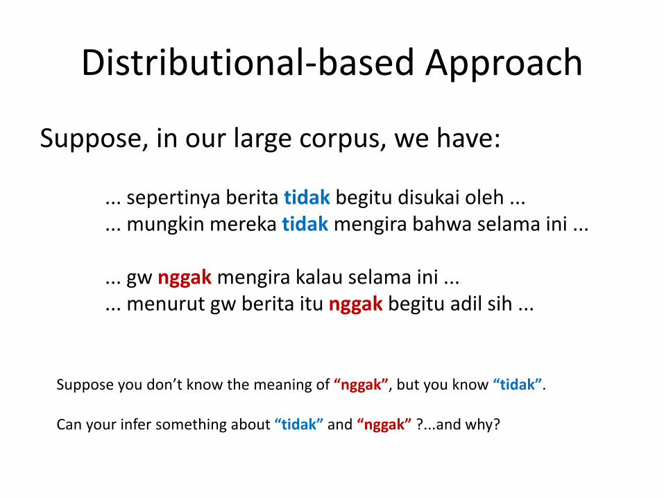
Suppose, in our large corpus, we have:
... sepertinya berita tidak begitu disukai oleh ...
... mungkin mereka tidak mengira bahwa selama ini ...
... gw nggak mengira kalau selama ini ...
... menurut gw berita itu nggak begitu adil sih ...
Suppose you don’t know the meaning of “nggak”, but you know “tidak”.
Can your infer something about “tidak” and “nggak” ?...and why?

Why Word Embeddings?
• Word representations are a critical component of manyNLP systems. It is common to represent words asindices in a vocabulary, but this fails to capture the richrelational structure of the lexicon.– Representing words as unique, discrete ids furthermore
leads to data sparsity, and usually means that we mayneed more data in order to successfully train statisticalmodels
• Vector-based models do much better in this regard.They encode continuous similarities between words asdistance or angle between word vectors in a high-dimensional space.

Why Word Embeddings?
• Can capture the rich relational structure of the lexicon
https://www.tensorflow.org/tutorials/word2vec

Word Embeddings
• Any technique that maps a word (or phrase) from it’s originalhigh-dimensional sparse input space to a lower-dimensionaldense vector space.
• Vectors whose relative similarities correlate with semanticsimilarity
• Such vectors are used both as an end in itself (for computingsimilarities between terms), and as a representational basisfor downstream NLP tasks, such as POS tagging, NER, textclassification, etc.

Continuous Representation of Words
• In research on Information Retrieval and Topic Modeling– Simple Vector Space Model (Sparse)– Latent Semantic Analysis– Probabilistic LSA– Latent Dirichlet Allocation
• [Distributional Semantic]– VSMs, LSA, SVD, etc.– Self Organizing Map– Bengio et al’s Word Embedding (2003)– Mikolov et al’s Word2Vec (2013)– Pennington et al’s GloVe (2014)
The first use neural “word embedding”
“word embedding” becomes popular!

Continuous Representation of Words
The Differences:
• In information retrieval, LSA and topic modelsuse documents as contexts.
– Capture semantic relatedness (“boat” and “water”)
• Distributional semantic models use words ascontexts (more natural in linguistic perspective)
– Capture semantic similarity (“boat” and “ship”)
Word Embedding

Distributional Semantic Models
Other classification based on (Baroni et al., ACL 2014)
• Count-based models– Simple VSMs
– LSA
– Singular Value Decomposition (Golub & VanLoan, 1996)
– Non-negative Matrix Factorization (Lee & Seung, 2000)
• Predictive-based models (neural network)– Self Organizing Map
– Bengio et al’s Word Embedding (2003)
– Mikolov et al’s Word2Vec (2013)
Baroni et la., “Don’t count, predict! A systematic comparison of context-counting vs. context-predicting semantic vectors”. ACL 2014

DSMs or Word Embeddings
• Count-based model
– first collecting context vectors and then reweightingthese vectors based on various criteria
• Predictive-based model (neural network)
– vector weights are directly set to optimally predict thecontexts in which the corresponding words tend toappear
– Similar words occur in similar contexts, the systemnaturally learns to assign similar vectors to similarwords.

DSMs or Word Embeddings
• There is no need for deep neural networks in orderto build good word embeddings.
– the Skipgram and CBoW models included in the word2veclibrary – are shallow neural networks
• There is no qualitative difference between(current) predictive neural network models andcount-based distributional semantics models.
– they are different computational means to arrive at thesame type of semantic model
https://www.gavagai.se/blog/2015/09/30/a-brief-history-of-word-embeddings/

Vector Space Model
Term-Document Matrix
D1 D2 D3 D4 D5
ekonomi 0 1 40 38 1
pusing 4 5 1 3 30
keuangan 1 2 30 25 2
sakit 4 6 0 4 25
inflasi 8 1 15 14 1
Vector of D2 = [1, 5, 2, 6, 1]
Each cell is the count of word t in document d

Vector Space Model
Term-Document Matrix
D1 D2 D3 D4 D5
ekonomi 0 1 40 38 1
pusing 4 5 1 3 30
keuangan 1 2 30 25 2
sakit 4 6 0 4 25
inflasi 8 1 15 14 1
Two documents are similar if they have similar vector!D3 = [40, 1, 30, 0, 15]D4 = [38, 3, 25, 4, 14]
Each cell is the count of word t in document d

Vector Space Model
Term-Document Matrix
D1 D2 D3 D4 D5
ekonomi 0 1 40 38 1
pusing 4 5 1 3 30
keuangan 1 2 30 25 2
sakit 4 6 0 4 25
inflasi 8 1 15 14 1
Vector of word “sakit” = [4, 6, 0, 4, 25]
Each cell is the count of word t in document d

Vector Space Model
Term-Document Matrix
D1 D2 D3 D4 D5
ekonomi 0 1 40 38 1
pusing 4 5 1 3 30
keuangan 1 2 30 25 2
sakit 4 6 0 4 25
inflasi 8 1 15 14 1
Two words are similar if they have similar vector!pusing = [4, 5, 1, 3, 30]sakit = [4, 6, 0, 4, 25]
Each cell is the count of word t in document d

Vector Space Model
Term-Context Matrix• Previously, we use entire Documents as our Context of word
– document-based models capture semantic relatedness (e.g. “boat” –“water”), NOT semantic similarity (e.g. “boat” – “ship”)
• We can get precise vector representation of word (forsemantic similarity task) if we use smaller context, i.e, Wordsas our Context!– Window of N words
• A word is defined by a vector of over counts of contextwords.

Vector Space Model
Sample context of 4 words ...
No Potongan konteks 4 kata
1 ... kekuatan ekonomi dan inflasi ...
2 ... obat membuat sakit pusing ...
3 ... sakit pening di kepala ...
4 ... keuangan menipis serta inflasi ...
5 ...

Vector Space Model
Term-Context Matrix
• Sample context of 4 words ...
ekonomi obat sakit kepala keuangan ...
inflasi 2 0 0 0 3 ...
pusing 0 1 6 6 1 ...
pening 0 2 6 6 0 ...
keuangan 2 0 0 0 4 ...
...
Two words are similar in meaning if they have similar context vector!Context Vector of “pusing” = [0, 1, 6, 6, 1, ...]Context Vector of “pening” = [0, 2, 6, 6, 0, ...]

Vector Space Model
• Weighting: it practically works well... instead ofjust using raw counts.
• For Term-Document matrix
– We usually use TF-IDF, instead of Raw Counts (onlyTF)
• For Term-Context matrix
– We usually use Pointwise Mutual Information (PMI)

Word Analogy Task
• Father is to Mother as King is to _____ ?
• Good is to Best as Smart is to _____ ?
• Indonesia is to Jakarta as Malaysia is to ____ ?
• It turns out that the previous Word-Context based vector model is good for such analogy task.
Mikolov, T., Chen, K., Corrado, G., & Dean, J. (2013). Distributed Representations of Words and Phrases and their Compositionality. NIPS, 1–9
Vking – Vfather + Vmother = Vqueen

Word Embeddings for Information Retrieval
• The two passages are indistinguishable for the query term “Albuquerque”!– Both contains the same
number of “Albuquerque”, i.e. Only one!
• Word embeddings can help us to distinguish them!
• Which one is the real one talking about “Albuquerque”??– #terms in the document
related to “Albuquerque”
Nalisnick et al., “Improving Document Ranking with Dual Word Embedding”, WWW 2016

Some basics …

Gradient Descent (GD)Problem: carilah nilai x sehingga fungsi f(x) = 2x4 + x3 – 3x2
mencapai titik local minimum.
Misal, kita pilih x dimulai dari x=2.0:
Local minimum
Algoritma GD konvergenpada titik x = 0.699, yang merupakan local minimum.

Gradient Descent (GD)
Algorithm:
"")()(
""
int"")('
)('
:...,,2,1
1
1
1
1
max
divergingreturnthenxfxfIf
valuexonconvergedreturnthenxxIf
pocriticalonconvergedreturnthenxfIf
xfxx
NtFor
tt
tt
t
tttt
αt : learning rate atau step size pada iterasi ke-tϵ: sebuah bilangan yang sangat kecilNmax: batas banyaknya iterasi, atau disebut epoch jika iterasi selalu sampai akhir
Algoritma dimulai dengan menebak nilai x1 !
Tips: pilih αt yang tidak terlalu kecil, juga tidak terlalu besar.

Gradient Descent (GD)Kalau parameter-nya ada banyak ?
Carilah θ = θ1, θ2, …, θn sehingga f(θ1, θ2, …, θn) mencapai localminimum !
)(
)(
)(
:
)(
)(
)()1(
)(
)(
2
)(
2
)1(
2
)(
)(
1
)(
1
)1(
1
t
t
n
t
t
n
t
n
t
tt
tt
t
tt
tt
f
f
f
convergednotwhile
Dimulai dengan menebaknilai awal θ = θ1, θ2, …, θn

Multilayer Neural Network (Multilayer Perceptron)
Misal, ada 3-layer NN, dengan 3 input unit, 2 hidden unit,dan 2 output unit.
x1
x2
x3
+1
+1
𝑊11(1)
𝑊21(1)
𝑊12(1)
𝑊22(1)
𝑊13(1)
𝑊23(1)
𝑏1(1) 𝑏2
(1)
𝑊11(2)
𝑊12(2)
𝑊21(2)
𝑊22(2)
𝑏1(2) 𝑏2
(2)
W(1), W(2), b(1), b(2) adalah parameter !

Multilayer Neural Network (Multilayer Perceptron)
Misal, untuk activation function, kita gunakan fungsihyperbolic tangent.
Untuk menghitung output di hidden layer:
)tanh()( xxf
)1(
23
)1(
232
)1(
221
)1(
21
)2(
2
)1(
13
)1(
132
)1(
121
)1(
11
)2(
1
bxWxWxWz
bxWxWxWz
)(
)(
)2(
2
)2(
2
)2(
1
)2(
1
zfa
zfa
Ini hanyalah perkalian matrix !
)1(
2
)1(
1
3
2
1
)1(
23
)1(
22
)1(
21
)1(
13
)1(
12
)1(
11)1()1()2(
b
b
x
x
x
WWW
WWWbxWz

Multilayer Neural Network (Multilayer Perceptron)
Jadi, Proses feed-forward secara keseluruhan hinggamenghasilkan output di kedua output unit adalah:
)(ax )(
)(
)3()3(
,
)2()2()2()3(
)2()2(
)1()1()2(
zsoftmaxh
baWz
zfa
bxWz
bW
i
(3)
i
(3)
i(3)
i)exp(z
)exp(za
f
softmax
Par: W(1)
Par: W(2)
Par: b(1)
Par: b(2)
x
a(3)

Multilayer Neural Network (Multilayer Perceptron)
Learning
Misal, Cost function kita adalah cross-entropy loss:
m adalah banyaknya training examples.
1
1 1 1
2)(
,
1
,
1
)(2
)(log1
),(l l ln
l
s
i
s
j
l
jiji
m
i Cj
ji Wpym
bWJ
Regularization terms

Multilayer Neural Network (Multilayer Perceptron)
Learning
Batch Gradient Descent
inisialisasi W, b
while not converged :
),(
),(
)(
)()(
)(
)()(
bWJb
bb
bWJW
WW
l
i
l
i
l
i
l
ij
l
ij
l
ij
Bagaimana cara menghitung gradient ??
Backpropagation Algorithm

Neural Language Model (Bengio et al., 2003)

Main Goal: Language Model
Actually, their main goal is to develop a language model, i.e., conditionalprobability of the next word given all the previous ones:
So that, we can compute the likelihood of a whole document or sentence bythe product of the probabilies each word given its previous words:
Given a document or sentence
)...|( 1221 wwwwwP ttt
T
t
ttTT wwwwPwwwwP1
121121 )...|()...(
TT wwwww ,,...,,, 1321

N-Gram Language Model
In N-Gram language model, we often relax the conditionalprobability of a word into just its n-1 previous words (MarkovAssumption):
For example, using Bi-Gram:
Using MLE, we can estimate the parameter using FrequencyCounts:
)...|()...|( 1111 nttttt wwwPwwwP
)|()|()|()|()|(
),,,(
embeddingendPwordembeddingPlearnwordPilearnPstartiP
embeddingwordlearniP
)...(
)...()...|(
11
1111
ntt
ntttnttt
wwcount
wwwcountwwwP

Problem with N-Gram
• There should be much more information in the sequence thatimmediately precedes the word to predict than just theidentity of the previous couple of words.
• It’s NOT taking into account the “similarity” between words.
• For example, in the training data:
• Then, the model should generalize for the following sentence:
The cat is walking in the bedroom
A dog was running in a room
WHY ? Dog-Cat, The-A, Bedroom-Room have similar semantic and grammatical roles !

Neural Language Model
Given a document or sentence
Where each word belongs to a Vocabulary,
We want to learn good model for:
TT wwwww ,,...,,, 1321
Vwi
Vj
j
t
t
ntttnttt
contextwscore
contextwscore
contextwscoresoft
wwwPwwwf
)),(exp(
)),(exp(
)),(max(
)...|(),...,,( 1111
11,..., tnt wwcontext

Neural Language Model
))(),...,(,(
)|(),...,,(
11
11
ntt
tntt
wCwCig
contextiwPwwif
We have Embedding/Projection Matrix
g is a neural network function.
mVC ||
m is size of word vector.
mRiC )(
C(i) is a function that maps A Word i into Its Vector
......
......
......
......
||V
m
Score for a particular output:

Merge (concat vector)
......
......
......
......
||V
m
1ntw 2tw 1tw
Feed-Forward Process
tanh
softmax
Par: C
Par: H
Par: W
Par: U
Par: d
Par: b
Vi
i
w
nttty
ywwwP t
)exp(
)exp()...|( 11
)tanh( HxdUWxbytw
))(),...,(( 11 ntt wCwCconcatx
Total Parameters:
),,,,,( CHUWdb
mnh
mnV
mV
hV
RH
RW
RC
RU
)1(
)1(||
||
||
||VRb
hRd
)...|( 11 nttt wwwP
Output Layer
Hidden Layer
ProjectionLayer
InputLayer

Merge (concat vector)
......
......
......
......
||V
m
1ntw 2tw 1tw
Training
tanh
softmax
Par: C
Par: H
Par: W
Par: U
Par: d
Par: b
How? We can use Gradient Ascent!
Iterative update using the following formula:
Training is achieved by looking θ that maximizes the following Cost Function:
Given training data TT wwwww ,,...,,, 1321
T
t
ntttT RwwwfT
wwJ1
111 )();,...,,(log1
);...(
Regularization terms
);...(: 1
T
oldnew wwJ
Learning rate
)...|( 11 nttt wwwP
Output Layer
Hidden Layer
ProjectionLayer
InputLayer

Where are the Word Embeddings?
• The previous model actually aims at building thelanguage model.
– So, where is the Word Embedding model that we need?
• The answer is: If you just need the WordEmbedding model, you just need the matrix C

Where are the Word Embeddings?
• After all parameters (including C) are optimized, thenwe can use C to map a word into its vector !
......
......
......
......
||V
m
mVRC ||
A Word w
Vw
mRwC )(
76.0
31.0
2.0
)(
wC

Problem?
Merge (concat vector)
......
......
......
......
||V
m
1ntw 2tw 1tw
tanh
softmax
Par: C
Par: H
Par: W
Par: U
Par: d
Par: b
)...|( 11 nttt wwwP
Computation in this area is very COSTLY!
Size of Vocabulary can reach 100.000 !
(Mikolov et al., 2013)Computational Complexity of this model per each training sample:
|)|()()( VhhmNmNQ
Dominating Term!
Composition of projection layerN words X size of vector m
Between projection layer & hidden layer

Word2Vec (Mikolov et al., 2013)

Word2Vec
• One of the most popular Word Embedding modelsnowadays!
• Computationally less expensive compared to theprevious model
• There are two types of models:
– Continuous Bag of Words Model (CBOW)
– Skip-Gram Model

Continuous Bag-of-Words
• Bengio’s language model onlylooks at previous words as acontext for predictions.
• Mikolov’s CBOW looks at n wordsbefore and after the target words.– Non-linear hidden layer is also
removed.
– All word vectors get projected into thesame position (their vectors areaveraged)
• “Bag-of-Words” is because theorder of words in the history doesnot influence the projection.
)......|( 11 ntttntt wwwwwP We seek a model for

Continuous Bag-of-Words
Merge (average)
......
......
......
......
||V
m
ntw 1tw ntw
ProjectionLayer
InputLayer
1tw
softmax
Feed-Forward Process
Vi
i
w
ntttntty
ywwwwwP t
)exp(
)exp()......|( 11
Wxbytw
))(),(),...,(),(( 11 ntttnt wCwCwCwCaveragex
Total Parameters:
),,( CWb
)...|( 11 ntttntt wwwwwP
Par: W
Par: b
Par: C
mnV
mV
RW
RC
)2(||
||
OutputLayer

Continuous Bag-of-Words
Merge (average)
......
......
......
......
||V
m
ntw 1tw ntw
ProjectionLayer
InputLayer
1tw
softmax
Training)...|( 11 ntttntt wwwwwP
Par: W
Par: b
Par: C
Training is achieved by looking θ that maximizes the following Cost Function:
Given training data TT wwwww ,,...,,, 1321
T
t
ntttnttT RwwwwwPT
wwJ1
111 )()......|(log1
);...(
Regularization terms
OutputLayer

Continuous Bag-of-Words
Merge (average)
......
......
......
......
||V
m
ntw 1tw ntw
ProjectionLayer
InputLayer
1tw
Hierarchical Softmax
Training)...|( 11 ntttntt wwwwwP
Actually, if we use vanilla softmax, then the computational complexity is still costly.
|)|()2( VmmNQ
OutputLayer
To solve this problem, they use Hierarchical Softmax layer. This layer uses a binary tree representation of the output layer with |V| units.
|))log(|()2( 2 VmmNQ
(Morin & Bengio, 2005)

Skip-Gram
• Instead of predicting the currentword based on the context, it triesto maximize classification of a wordbased on another word in thesame sentence.
• Use each current word as an inputto a log-linear classifier withcontinuous projection layer, andpredict words within a certainrange before and after the currentword.
We seek a model for )|( tjt wwP

Skip-Gram
......
......
......
......
||V
m
tw
ProjectionLayer
InputLayer
softmax
)|( tjt wwP
Par: W
Par: b
Par: C
OutputLayer
Feed-Forward Process
Vi
i
w
tjty
ywwP
jt
)exp(
)exp()|(
Wxbyjtw
)( twCx
Total Parameters:
),,( CWb
mV
mV
RW
RC
||
|| ||VRb

Skip-Gram
......
......
......
......
||V
m
tw
ProjectionLayer
InputLayer
softmax
)|( tjt wwP
Par: W
Par: b
Par: C
OutputLayer
Training
Training is achieved by looking θ that maximizes the following Cost Function:
Given training data TT wwwww ,,...,,, 1321
T
t jcjc
tjt
T
RwwPT
wwJ
1 0,
1
)()|(log1
);...(
Regularization Terms
c is the maximum distance of the words, or WINDOW size

Skip-Gram
How to develop dataset?
For example, let’s consider the following dataset:
the quick brown fox jumped over the lazy dog
Using c = 1 (or window = 1), we then have dataset:
([the, brown], quick), ([quick, fox], brown), ([brown, jumped], fox), ...
Therefore, our (input, output) dataset becomes:
(quick, the), (quick, brown), (brown, quick), (brown, fox), ...
Reference: https://www.tensorflow.org/tutorials/word2vec
Use this dataset to learn
So that, the cost function is optimized!
)|( tjt wwP
T
t jcjc
tjtT wwPT
wwJ1 0,
1 )|(log1
);...(
)|( 1 quickwbrownwP tt For example,

Skip-Gram
......
......
......
......
||V
m
tw
ProjectionLayer
InputLayer
Hierarchical Softmax
)|( tjt wwP
Par: C
OutputLayer
Training
Actually, if we use vanilla softmax, then the computational complexity is still costly.
|)|( VmmCQ
To solve this problem, they use Hierarchical Softmax layer. This layer uses a binary tree representation of the output layer with |V| units.
|))log(|( 2 VmmCQ
(Morin & Bengio, 2005)

Word2Vec + H-Softmax + Noise Contrastive Estimation (Mikolov et al., 2013)

Previously
• Standard CBOW and Skip-gram models use standard flat softmax layer inthe output.
• This is very expensive, because we need to compute and normalize eachprobability using the score for all other words in the Vocabulary in thecurrent context, at every training step.
SOURCE: https://www.tensorflow.org/tutorials/word2vec
This picture is only CBOW.

Solution?
• In the first paper, Mikolov et al. (2013) use HierarchicalSoftmax Layer (Morin & Bengio, 2005).
• H-Softmax replaces the flat softmax layer with a hierarchicallayer that has the words as leaves.
• This allows us to decompose calculating the probability of oneword into a sequence of probability calculations, which savesus from having to calculate the expensive normalization overall words.
Sebastian Ruder. On word embeddings - Part 2: Approximating the Softmax. http://sebastianruder.com/word-embeddings-softmax

H-Softmax
• We can reason that at a tree's root node (Node 0), the probabilities of branchingdecisions must sum to 1.
• At each subsequent node, the probability mass is then split among its children,until it eventually ends up at the leaf nodes, i.e. the words.
Sebastian Ruder. On word embeddings - Part 2: Approximating the Softmax. http://sebastianruder.com/word-embeddings-softmax
We can now calculate theprobability of going right(or left) at a given node ngiven the context c.
vn is embedding in node n.
).(),|( nvWcnrightP
),|(1),|( cnrightPcnleftP

H-Softmax
• The probability of a word w given its context c, is then simply the product of theprobabilities of taking right and left turns respectively that lead to its leaf node.
Sebastian Ruder. On word embeddings - Part 2: Approximating the Softmax. http://sebastianruder.com/word-embeddings-softmax
(Hugo Lachorelle's Youtube lectures)
https://www.youtube.com/watch?v=B95LTf2rVWM

Noise Contrastive Estimation (NCE)
• In their second paper, the CBOW and skip-gram models are instead trainedusing a binary classification objective (logistic regression) to discriminatethe real target words wt from k imaginary (noise) words w.
NCE in the output layer, for CBOW.
SOURCE: https://www.tensorflow.org/tutorials/word2vec