word and speaker recognition system
TRANSCRIPT
ii
WORD AND SPEAKER RECOGNITION SYSTEM
By
TAN SHWU FEI
DISSERTATION REPORT
Submitted to the Electrical & Electronics Engineering Programme
in Partial Fulfillment of the Requirements
for the Degree
Bachelor of Engineering (Hons)
(Electrical & Electronics Engineering)
Universiti Teknologi PETRONAS
Bandar Seri Iskandar
31750 Tronoh
Perak Darul Ridzuan
Copyright 2010
by
Tan Shwu Fei, 2010

iii
CERTIFICATION OF APPROVAL
WORD AND SPEAKER RECOGNITION SYSTEM
by
Tan Shwu Fei
Dissertation report is submitted to the
Electrical & Electronics Engineering Programme
Universiti Teknologi PETRONAS
in partial fulfilment of the requirement for the
Bachelor of Engineering (Hons)
(Electrical & Electronics Engineering)
Approved:
__________________________
Assoc. Prof. Dr. Mohammad Awan
Project Supervisor
UNIVERSITI TEKNOLOGI PETRONAS
TRONOH, PERAK
December 2010

iv
CERTIFICATION OF ORIGINALITY
This is to certify that I am responsible for the work submitted in this project,
that the original work is my own except as specified in the references and
acknowledgements, and that the original work contained herein have not been
undertaken or done by unspecified sources or persons.
__________________________
Tan Shwu Fei

v
ABSTRACT
In this report, a system which combines user dependent Word
Recognition and text dependent speaker recognition is described. Word
recognition is the process of converting an audio signal, captured by a
microphone, to a word. Speaker Identification is the ability to recognize a
person identity base on the specific word he/she uttered. A person's voice
contains various parameters that convey information such as gender, emotion,
health, attitude and identity. Speaker recognition identifies who is the speaker
based on the unique voiceprint from the speech data. Voice Activity Detection
(VAD), Spectral Subtraction (SS), Mel-Frequency Cepstrum Coefficient
(MFCC), Vector Quantization (VQ), Dynamic Time Warping (DTW) and k-
Nearest Neighbour (k-NN) are methods used in word recognition part of the
project to implement using MATLAB software. For Speaker Recognition part,
Vector Quantization (VQ) is used. The recognition rate for word and speaker
recognition system that was successfully implemented is 84.44% for word
recognition while for speaker recognition is 54.44%.

vi
ACKNOWLEDGEMENT
I would like to acknowledge the following people for their support and
assistance with this project.
I would like to convey my deepest appreciation towards my final year
project supervisor, Assoc. Prof. Dr. Mohammad Awan who has persistently
and determinedly assisted me during the project. It would have been very
arduous to complete this project without the passionate supports and guidance
encouragement and advices given by him.
Second, I would like to thank to Universiti Teknologi PETRONAS
(UTP) and Electrical Engineering for providing us theoretical knowledge
which can be applied in our Final Year Project.
Lastly, I would love to thank the people that have been giving me
morale support all the way through the time I was doing the project. Thank you.

vii
TABLE OF CONTENTS
ABSTARCT………………………………………………………………….. v
ACKNOWLEDGEMENT…………………………………………………...vi
LIST OF FIGURE…………………………………………………………… x
LIST OF TABLES………………………………………………………… xii
LIST OF ABBREVIATIONS ......................................................................... xiii
CHAPTER 1 INTRODUCTION ...................................................................... 1
1.1 Background of Study ............................................................... 1
1.2 Problem Statement ................................................................... 9
1.3 Objective and Scope of Study ............................................... 11
1.4 Conclusion ............................................................................. 11
CHAPTER 2 LITERATURE REVIEW ........................................................ 12
2.1 Literature review on Word/Speech Recognition ................... 13
2.1.1 In 1950s ......................................................................... 13
2.1.2 In 1960s ......................................................................... 13
2.1.3 In 1970s ......................................................................... 14
2.1.4 In 1980s ......................................................................... 14
2.1.5 In 1990s ......................................................................... 14
2.1.6 In 2000s ......................................................................... 15
2.2 Literature Review on Speaker Recognition ........................... 15
2.2.1 In 1960s and 1970s ....................................................... 15
2.2.2 In 1980s ......................................................................... 16
2.2.3 In 1990s ......................................................................... 16
2.2.4 In 2000s ......................................................................... 17
2.3 Features Attraction Technique ............................................... 17
2.3.1 Linear Predictive Coding (LPC) ................................... 17
2.3.2 Perceptual Linear Prediction (PLP) ............................. 18
2.3.3 Mel-Frequency Cepstrum Coefficient(MFCC) ............. 18

viii
2.4 Pattern Recognition ............................................................... 19
2.4.1 Hidden Markov Model (HMM) ..................................... 20
2.4.2 Neural Network (NN) .................................................... 21
2.4.3 Vector Quantization (VQ) ............................................. 22
2.5 Conclusion ............................................................................. 23
CHAPTER 3 METHODOLOGY ................................................................... 24
3.1 Overview Planning ................................................................ 24
3.2 Tools and Equipment ............................................................. 27
3.2.1 Software ........................................................................ 27
3.3 Project Flow in MATLAB ..................................................... 28
3.4 Research Methodology .......................................................... 29
3.4.1 Front End Processing ................................................... 30
3.4.1.1 Voice Activity Detection (VAD) .................... 30
3.4.1.2 Spectral Subtraction (SS) ................................ 35
3.4.1.3 Mel-Frequency Cepstrum Coefficient (MFCC)38
3.4.1.4 Cepstrum ......................................................... 42
3.4.2 Word Recognition ......................................................... 43
3.4.2.1 Dynamic Time Warping (DTW) ..................... 43
3.4.2.2 k-Nearest Neighbour(k-NN) ............................ 45
3.4.3 Speaker Recognition ..................................................... 47
3.4.3.1 Vector Quantization (VQ) ............................... 47
3.5 Conclusion ............................................................................. 52
CHAPTER 4 RESULT AND DISCUSSION ................................................. 53
4.1 Word Recognition .................................................................. 54
4.2 Speaker Recognition .............................................................. 57
4.3 Miscellaneous ........................................................................ 61
4.4 Conclusion ............................................................................. 68
ix
CHAPTER 5 CONCLUSION AND RECOMMENDATIONS .................... 69
5.1 Conclusion ............................................................................. 69
5.2 Recommendation ................................................................... 70
REFERENCES ................................................................................................. 71
APPENDICES ............................................................................. 76
Appendix A GANTT CHART FYP I .......................................... 77
Appendix B GANTT CHART FYP II....……………………. ..77
Appendix C ENGINEERING DESIGN EXHIBITION……….78
Appendix D NOTIFICATION OF ACCEPTED PAPER BY
ICSTE 2011……………………………………....80
Appendix E CONFERENCE PAPER………………………….83

x
LIST OF FIGURES
Figure 1 How the Word Being Recognized [2] ...................................................4
Figure 2 Overview of Speaker Recognition ........................................................5
Figure 3 Basic Structure of Speaker Identification .............................................6
Figure 4 Basic Structure of Speaker Verification ...............................................6
Figure 5 Recognition Process ..............................................................................8
Figure 6 Block Diagram of Pattern Recognition Speech Recognizer ...............19
Figure 7 A 3-State Markov Chain with Transition Probabilities by Hansen [30]
....................................................................................................................20
Figure 8 Flow Chart for FYP I ..........................................................................25
Figure 9 Flow Chart for FYP II .........................................................................26
Figure 10 Process flows of the Speaker Recognition and Word Recognition ..28
Figure 11 Flow Chart for VAD .........................................................................31
Figure 12 Beginning and Endpoint by using energy alone [33] ........................33
Figure 13 Beginning and Endpoint by using both energy and ZCR [33] .........34
Figure 14 SS algorithm block diagram ..............................................................35
Figure 15 Block Diagram of the MFCC Processor [36] ...................................38
Figure 16 256 points hamming window [36] ....................................................40
Figure 17 Mel filter bank operating on a spectrum [36] ...................................41
Figure 18 The Mel spcaed filer banks, acting in the frequency domain [36] ....42
Figure 19 Time Alignment of two time-dependent sequences [38] ..................43
Figure 20 k-NN classifications ..........................................................................45
Figure 21 Flow Chart for k-NN Algorithm .......................................................46
Figure 22 Flow Diagram of VQ-LBG Algorithm [41] ......................................48
Figure 23 Overview of Speaker Recognition Algorithm (Part 1) .....................50
Figure 24 Overview of Speaker Recognition Algorithm (Part 2) .....................51
Figure 25 Database over the volume limit ........................................................61
Figure 26 Database within the volume limit .....................................................62
Figure 27 Original waveform for word "One" ..................................................63

xi
Figure 28 Waveform after VAD .......................................................................64
Figure 29 Waveform after SS ............................................................................65
Figure 30 MFCC Coefficient ............................................................................66
Figure 31 MFCC coefficient of the input speech ..............................................67
Figure 32 Test words for One by original speech, One by different person,
Two, Three (From left to right) .........................................................67

xii
LIST OF TABLES
Table 1 Word Recognition using DTW.............................................................54
Table 2 Word Recognition using VQ ................................................................55
Table 3 Word Recognition using DTW and VQ ...............................................56
Table 4 Speaker Recognition using DTW .........................................................57
Table 5 Speaker Recognition using VQ ............................................................58
Table 6 Speaker Recognition after combined with Word Recognition .............59
Table 7 Overall of Recognition Rate .................................................................60
xiii
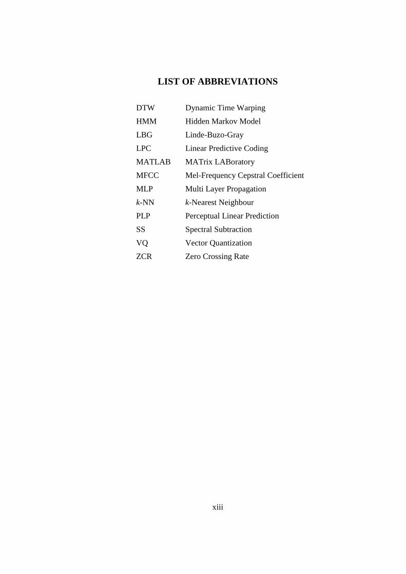
LIST OF ABBREVIATIONS
DTW Dynamic Time Warping
HMM Hidden Markov Model
LBG Linde-Buzo-Gray
LPC Linear Predictive Coding
MATLAB MATrix LABoratory
MFCC Mel-Frequency Cepstral Coefficient
MLP Multi Layer Propagation
k-NN k-Nearest Neighbour
PLP Perceptual Linear Prediction
SS Spectral Subtraction
VQ Vector Quantization
ZCR Zero Crossing Rate
1
Chapter 1
INTRODUCTION
By using speech to communicate in our daily life become very simple
until human tend to forget how inconsistent a signal speech is. Word and
Speaker recognition become more and more important in allowing or denying
access to restrict data or facilities [1]. Word recognition system is a system that
can recognize a word. Speaker recognition system is a system that can
recognize who the speaker is. Word recognition mean that the computer can
take dictation but do not understand what is being said. Speaker recognition is
related to Speech recognition [2]. Instead of determine what was said, it finds
out who said it. The combination of these two systems is a very active research
nowadays.
1.1 Background of Study
One of the most fascinating characteristics of humans is their capability
to communicate or share their idea by means of speech. With these
advantages, the possibility of creating machines capable to recognize and
understand what you say would provide a comfortable and natural way of
communication. If this applies to your personal computer, it can reduce the
amount of typing, leave your hands free, and allow you to move away from the
screen. This is called Speech Recognition which means the ability to identify
spoken word. Instead of determine what you say, Speaker Recognition can
determine who said it. Speaker recognition is extracting, characterizing and
recognizing the information in the speech signal conveying speaker identity.
2
The performance of speech and speaker recognition system nowadays
are far from perfect but these system have proven their usefulness in some
application.
The mightiest invention of speech recognition system is the use for the
primary purpose of aiding persons with disabilities. The Boeing Company has
a history of interest in speech recognition for use in aircraft. However, it was
also, perhaps unwittingly, instrumented in the use of speech recognition for the
seriously disabled. Some 20 years ago one of its programmers was rendered
quadriplegic from a boating accident. The group working on speech
recognition had several discrete-speech, speaker-dependent recognizers that
were unused at the time, so they developed a voice-controlled interface that
allowed the disabled programmer to operate his computer, control a robotic
arm for fetching manuals and turning their pages, and interface to a FORTRAN
development system so he could continue to work [3]. The system eventually
evolved into a robotic vocational workstation for the physically disabled
professional.
For some real-world application, Delco electronics employs IBM
PC/AT Cherry Electronics and Intel RMX86 recognition systems to collect
circuit board inspection data while the operator repairs and mark the boards.
Southern Pacific Railway inspectors now routinely use a PC-based Votan
recognition system to enter car inspection information from the field by walkie-
talkie. Besides, Michigan Bell has installed a Northern Telecom recognition
system to automate collect and third-number billed calls. AT&T has also put in
field trial systems to automate call type selection in its Reno, Nevada, and
Hayward, California, offices [2].
Speech Recognition may use in Telecommunication. For example,
voice access to a bank account by telephone. For command and control, it
happen in military parlance where officers in charge of an operation can issue
commands to control the movement and deployment of men and machines [4].

3
Speech Recognition can also be used in education for people to learn foreign
language by speak to the system can make sure the pronunciation is correct [5].
Speaker Recognition often use in security device to control access to building
or information. For example Texas Instruments corporate computer center
security system. Security Pacific has employed speaker verification as a
security mechanism on telephone-initiated transfers of large amount of money
[2].
More recent applications are for controlling access to computer
networks or website. Also used for automated password reset service. Besides,
some applications are home-parole monitoring and prison call monitoring.
There has also been discussion of using automatic systems to corroborate
aural/spectral inspections of voice samples for forensic analysis [6].
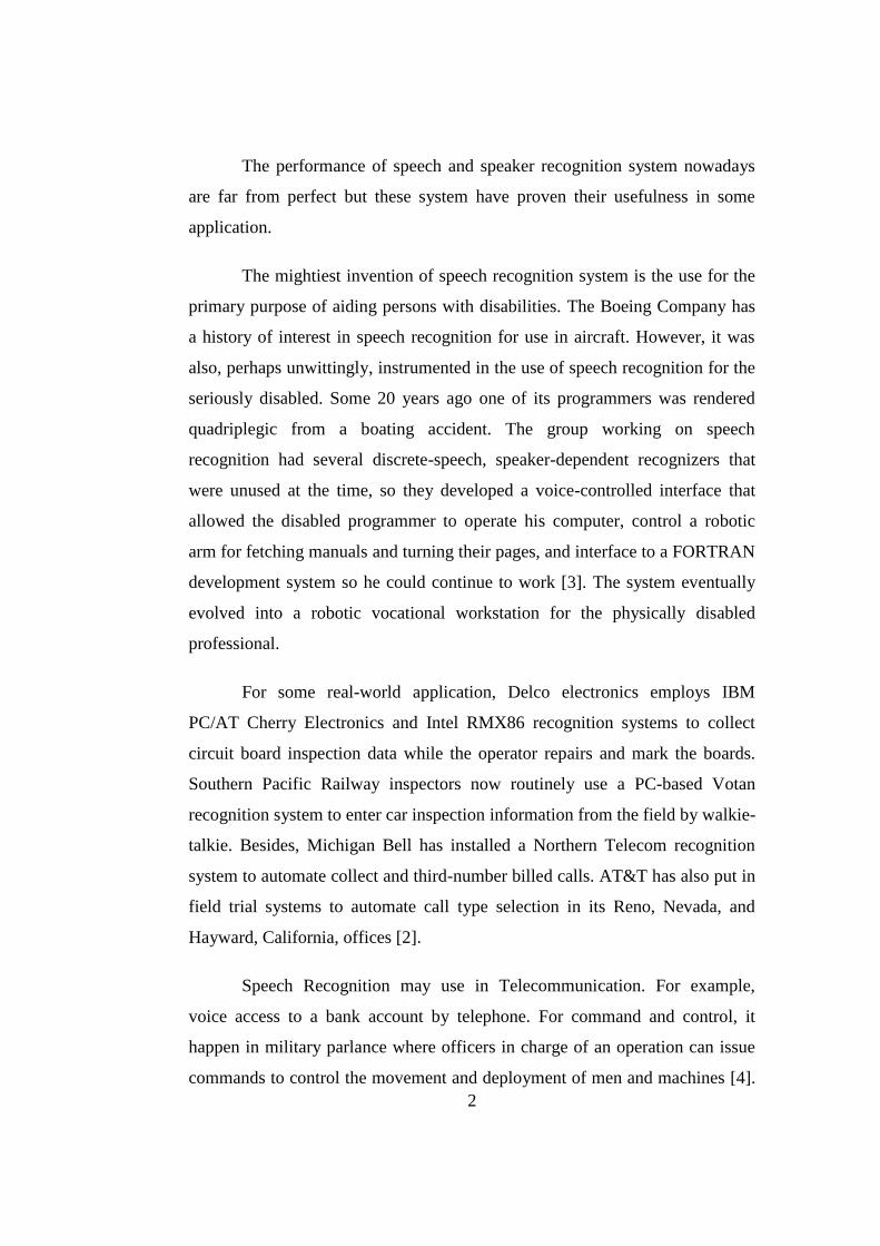
There are five main components need to pass through to recognize a
word. First, a reference speech patterns are stored as speech template or as
generative speech models. At another side, a speaker is speak to a microphone
and associated analog-to-digital converter are digitally encodes the raw speech
waveform. Then, MATLAB performs recognition to separate speech from non-
speech, speech enhancement by reducing noise and feature extraction. After
that preprocessed signal storage is used for the recognition algorithm. Once the
user‟s speech sample preprocessed by the MATLAB, the user‟s speech
database are compare to the stored reference patterns. Lastly the pattern
matching algorithm computes a measurement between the preprocessed signal
from the user‟s speech and all the stored database to choose the best match. [2]
Figure 1 show the flow of the how the word being recognized.
4
Figure 1 How the Word Being Recognized [2]
Most of us are aware of the fact that every human have different voice
vocal. With this important property, we are able to recognize a friend over a
telephone. No matter how we mimic the voice of someone, there are still some
different in energy, pronunciation and etc. Speaker recognition is the process of
automatically recognizing who is speaking on the basis of individual
information included in speech waves. Flow chart shown in Figure 2 shows the
overview of the Speaker Recognition.
Speech
Capture
Device
DSP
Module
Preprocessed
Signal
Storage
Reference
Speech
Patterns
Pattern-
Matching
Algorithm

5
Figure 2 Overview of Speaker Recognition
Speaker Recognition can be categorized in two categories: Speaker
Identification and Speaker Verification. Speaker Identification is a process of
finding the person‟s identity by matching the speech pattern on a set of known
speaker‟s voice in the database [7]. The system will choose the best matching
speaker. Speaker Verification is a process of accept or reject the person‟s voice
compare with the voice in the database. Speaker Identification with text
dependent method is the speaker require to speak a specific words while
Speaker Identification with text independent method is the speaker.
Speaker
Recognition
Speaker Identification
Choosing a
person‟s identity
from a set of known
speaker
Speaker
Verification
Accept / Reject
the person‟s
identity
Text Dependent
Require to
speak specific
words
Text Independent
Not require to
speak specific
words

6
Figure 3 Basic Structure of Speaker Identification
Figure 3 shows the Basic Structure of Speaker Identification. In
Speaker Identification, M speaker models are examining parallel. The most
likely one is chosen and the decision will be one of the speaker‟s ID in the
database, or will be „none of the above‟ if and only if the matching score is
below some threshold.
Figure 4 Basic Structure of Speaker Verification
Speaker
Database
Speaker Model
Front-end Processing
VAD
SS
MFCC
Decision Pattern
Matching
Front-end
Processing
VAD
SS
MFCC
Decision
Best
Selection
Speaker
Model
M
Speaker
Model 1
Speaker
Model 2
Speaker
Databas
e

7
By referring to Figure 4, the Basic Structure of Speaker Verification
there are three main components shown in the structure are: Front-end
Processing, Speaker Modeling, and Pattern Matching. Front-end processing is
performs when speaker speak to the system to get the feature vectors of
incoming voice, and then depending on the models used in Pattern Matching,
the match scores is calculated. If the score is larger than a certain threshold,
then as a result, claimed speaker would be acknowledged.
In this project, Speaker Identification text-dependent is conducted.
The program contains two functionalities: A training mode, a
recognition mode. Training mode can also called feature extraction while
recognition mode is feature matching. Feature extraction is same as the front
end processing of word recognition which is the process that extracts a small
amount of data from the voice signal that can later be used to represent each
speaker. Feature matching involves the actual procedure to identify the
unknown speaker by comparing extracted features from his/her voice input
with the ones from a set of known speakers. In the training phase, each
registered speaker has to provide samples of their speech so that the system can
build or train a reference model for that speaker. In the testing phase, the input
speech is matched with stored reference model(s) and a recognition decision is
made.
8
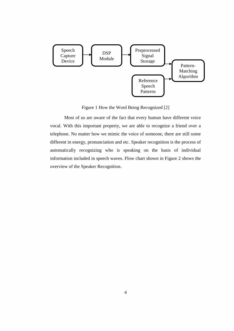
Figure 5 Recognition Process
According to Figure 5, the reference speech sample is the speech in the
database while test speech sample is the unknown speaker‟s voice. Both speech
samples are extracted from the speech utterance at features extraction stage. At
the training stage, reference speech samples are trained from the reference
patterns by various methods. Statistical parameters from the reference speech
data is formed for later used. At Pattern Matching stage, the test pattern is
compare with the reference pattern. After comparison, the test pattern is labeled
to a speaker model at the decision stage. The output with minimum risk is
produced.
Features
Extraction
Features
Extraction
Training
Pattern
Matching
Recognition
Decision
Recognition
Output
Reference
Speech
Sample
Test
Speech
Sample
9
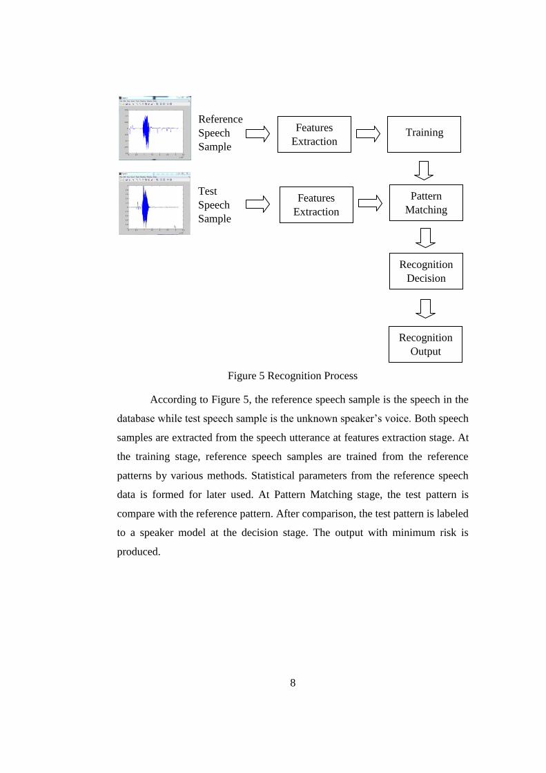
1.2 Problem Statement
Word and Speaker Recognition System is a very useful system to
develop on. The speaker-specific characteristics of speech are due to
differences in physiological and behavioral aspects of the speech production
system in humans. Speech is produce begins with a thought which shows the
initial communication message. Following the rules of the spoken language and
grammatical structure, words and phrases are selected and ordered. After the
thought constructs into language, brain sends commands by means of motor
nerves to the vocal muscles, which move the vocal organs to produce sound
[7]. There are a lot of existing word recognition or speaker recognition
standalone systems, however there are little research on combined word and
speaker recognition. With the word and speaker recognition system, security
feature using speaker recognition can be implemented on top of word
recognition- based applications.
The problems of the project involve in two parts. The first part is Word
Recognition while the second part is Speaker Recognition.
For the Word Recognition, the tasks to be completed are:
Record word from “one” to “nine” for as much speakers as possible in
a minimal interference and minimal noise environment and save it in a
file that can be used later on for processing.
Using the recorded data file and MATLAB speech processing tool box
find the “signature” of a word contents so that the word can be
recognized.
For Speaker Recognition, the tasks to be completed are:
Record words from more speakers and to design an algorithm or
method that can recognize who the speaker is.

10
Below are some complexities of Word and Speaker Recognition:
a) The system has to handle the variability of the speaker speech.
b) Speaking rate: The speed we induced a word is different every time we
speak it depending on the health, emotion and etc.
c) Vocabulary Size: Different size of vocabulary can be confused even
small vocabulary size.
d) Environment: Stationary or non-stationary noises, correlated noises
will affects the performance of the system.
Speech signals in training and testing sessions can be greatly different
due to many facts such as people voice change with time, health conditions (e.g.
the speaker has a cold), speaking rates, and so on. There are also other factors,
beyond speaker variability, that present a challenge to speaker recognition
technology. Examples of these are acoustical noise and variations in recording
environments (e.g. speaker uses different telephone handsets).
The problem of speaker recognition is pattern recognition which is to
classify the input speech into one of a number of categories or classes.
Furthermore, if there exist some set of patterns that the individual classes of
which are already known, then one has a problem in supervised pattern
recognition [5].
At the end the software package must also able to recognize at least a
common word and can also find out who the speaker is.
11
1.3 Objective and Scope of Study
The main aim of this project is to improve the word and speaker
recognition system, by enhancing the audio processing techniques.
The objectives are:
To understand the speaker recognition and word recognition methods.
To design and develop the speaker recognition and word recognition
algorithms on MATLAB.
To further improve the efficiency, robustness and reliability of the
system.
In this project, Word Recognition and text dependent Speaker
Recognition system has been conducted using MATLAB program.
1.4 Conclusion
Word and Speaker recognition can look forward to a promising future
both in terms of challenging research and useful application. Word and speaker
recognition besides help in security, it also help the hard-of hearing by giving
them printed text to read and the wheelchair-bound by following them to
control their vehicle by voice. It is a challenging in implementing this system.

12
Chapter 2
LITERATURE REVIEW
There is already five decades the attention of research in automatic
word and speaker recognition machine has drawn an enormous attention. A
large number of speech processing techniques have been proposed and
implemented, and a number of significant advances have been compared in this
field during the last one to two decades, which are aroused by the development
of algorithms, computational architectures and hardware. There are many
techniques have been developed by researchers in doing the word and speaker
recognition system. There are many challenges and research on word and
speaker recognition system before creating a machine that can communicate
naturally with people. In recent years, automatic word recognition has reached
a soaring of performance. Due to the improvement of the algorithm and
techniques used, the word-error rates dropping by a factor of five in the past
five years. With the development of speech recognition system, it has become
ordinary and is being used as an alternative for keyboards. Consequently, the
recognition rate of this system is improved especially when using a
combination of various algorithms and techniques [6].

13
2.1 Literature review on Word/Speech Recognition
Word/Speech recognition has been start implemented since 1950s. The
first speech recognizer appeared in 1952 and consisted of a device for the
recognition of single spoken digits.
2.1.1 In 1950s
In Bell Laboratories, a system that can recognize an isolated digit for a
single speaker is built. In year 1956, at RCA Laboratories, Olson and Bellar
tried to recognize 10 distinct syllables of a single speaker. [8] University
College in England, Fry and Denes tried to build a recognizer that can
recognize four vowels and nine consonants in year 1959 [9]. At the same year
Forgie and Forgie at MIT Lincoln Laboratories devised a system which was
able to recognize 10 vowels embedded in a /b/ - vowel - /t/ format in a speaker-
independent manner [10]. In the Soviet Union, Vintsyuk proposed the use of
dynamic programming methods for time aligning a pair of speech utterances
[11].
2.1.2 In 1960s
In continuous speech recognition, Reddy at Carnegie Mellon University
conducted a pioneering research in the field of continuous speech recognition
by dynamic tracking of phonemes [12]. At the same time, Martin and his
colleagues at RCA Laboratories developed a set of elementary time-
normalization methods, based on the ability to reliably detect speech starts and
ends, that significantly reduced the variability of the recognition scores [13].
Nagata and his colleagues at NEC Laboratories built a hardware digit
recognizer in 1963 [14].

14
2.1.3 In 1970s
Researchers on large vocabulary speech recognition for three distinct
tasks, namely the New Raleigh language for simple database queries at IBM
Lab. In AT&T Bell Labs there are researchers making speaker-independent
speech-recognition systems [15]. In 1973, one of the first demonstrations of
speech understanding was achieved by Carnegie Mellon University (CMU).
CMU‟s Harpy system was able to recognize speech using a vocabulary of
1,011 words with reasonable accuracy [16].
2.1.4 In 1980s
The problem of creating a robust system capable of recognizing a
fluently spoken string of connected word (e.g., digits) was a focus of research.
One of the key technologies developed in the 1980s is the hidden Markov
model (HMM) approach [17]. In the 1980s, the idea of applying neural
networks to speech recognition was reintroduced. Actually neural networks
were first introduced in the 1950s, but they did not prove useful because of
practical problems. A deeper understanding of the strengths and limitations of
the technology was achieved, as well as an understanding of the relationship of
this technology to classical pattern classification methods [18].
2.1.5 In 1990s
In the 1990s, there are different innovation pattern took place in the
field of pattern recognition. The problem of pattern recognition, which
traditionally the framework of Bayes is followed and required estimation of
distributions for the data, was transformed into an optimization problem
involving minimization of the experiential recognition error [19]. To against
the mismatch between training and testing conditions, various techniques were
investigated to increase the robustness of speech recognition systems The

15
mismatch is caused by background noises, voice individuality, microphones,
transmission channels, room reverberation, etc.
2.1.6 In 2000s
The Effective Affordable Reusable Speech-to-Text (EARS) program
was conducted to develop speech-to text (automatic transcription) technology.
Defense Advanced Research Projects Agency (DARPA), aim of achieving
substantially richer and much more accurate output than before. The system is
kept on improving to become more robust especially for spontaneous speech,
utterance verification and confidence measures are being intensively
investigated [20].
2.2 Literature Review on Speaker Recognition
After Word/Speech recognition has been implemented, Speaker
recognition system also had started at 1960s. Speaker recognition has a history
dating back some four decades and uses the acoustic features of speech that
have been found to differ between individuals.
2.2.1 In 1960s and 1970s
The first attempts for automatic speaker recognition were made in the
1960s, one decade later than that for automatic speech recognition. Doddington
at Texas Instruments (TI) replaced filter banks that use by Pruzansky at Bell
Labs [21] by formant analysis [22]. TI built the first fully automated large scale
speaker verification system providing high operational security. Verification
was based on a four-word randomized utterance built from a set of 16
monosyllabic words. The use of the combination of cepstral coefficient is
proposed by Furui [23] .The first and second polynomial coefficients as frame-
based features to increase robustness against distortions by the telephone

16
system. He had implemented an online system and tested it for a half year with
many calls by 120 users. The cepstrum-based features later became standard,
not only for speaker recognition, but also for speech recognition.
2.2.2 In 1980s
The Hidden Markov Model (HMM) -based text-dependent method was
introduced. The HMM that was used in the same way for word recognition is
the HMM that use in speaker recognition as well HMM. It has the same
advantages for speaker recognition as they do for word recognition. Vector
Quantization (VQ) /HMM-based text-independent method are introduced at the
same time. It has nonparametric and parametric probability models were
investigated for text-independent speaker recognition [24].
2.2.3 In 1990s
Research on increasing robustness of the speaker recognition system
became a central theme in the 1990s. Matsuiet al. compared the VQ-based
method with the discrete/continuous ergodic HMM based method, concentrated
on robustness against utterance variations [24]. They found that the continuous
ergodic HMM method is far better to the discrete ergodic HMM method and
that the continuous ergodic HMM method is as robust as the VQ. Text-
prompted speaker recognition method is propsed by Matsui et al. Text-
prompted speaker recognition is the key sentences are completely changed
every time the system is used [25]. This method not only accurately recognizes
speakers, but can also reject an utterance whose text differs from the prompted
text, even if it is uttered by a registered speaker.

17
2.2.4 In 2000s
High-level features such as word idiolect, pronunciation, phone usage,
prosody, etc. have been successfully used in text independent speaker
verification. There has been a lot of interest in audio-visual speaker verification
systems, in which a combination of speech and image information is used. The
audio-visual combination helps improve system reliability.
2.3 Features Attraction Technique
According to Martens (2000), there are various speech features
extraction techniques which are Linear Predictive Coding (LPC), Perceptual
Linear Prediction (PLP) and Mel-Frequency Cepstral Coefficient (MFCC).
However, MFCC has been the most frequently used technique especially in
speech recognition and speaker verification applications [26].
2.3.1 Linear Predictive Coding (LPC)
According to Huang et al. in year 2001, LPC is known as LPC analysis or
Auto-Regressive (AR) modeling. It is a very powerful method for speech
analysis; therefore, it is widely used. LPC is fast and simple, yet an effective
method for estimating the main parameters of speech signals. At the same year,
Felber said that LPC is useful and it can produce a set of coefficients that
describe a digital filter, which would together produce a sound similar to the
original speech. It is also able to extract and store time varying formant
information, where formants are points in a sound‟s spectrum where the
loudness is boosted.
In year 2003, Wai mention that based on a highly simplified model for
speech production, the linear prediction coding (LPC) algorithm is one of the
earliest standardized coders, which works at low bit-rate inspired by
18
observations of the basic properties of speech signals and represents an attempt
to mimic the human speech production mechanism [26].
2.3.2 Perceptual Linear Prediction (PLP)
In year 1990, another popular feature set is the set of perceptual linear
prediction (PLP) coefficients, which was first introduced by Hermansky. In
1999, Madisetti and Williams identified certain perceptual attributes and
properties of the human auditory system to be considered. Those perceptual
properties include the loudness, pitch, threshold of hearing, differential
threshold, masked threshold, and critical bands and peripheral auditory filters.
In 2005 Hönig et al. reported that PLP features are more robust when there is
an acoustic mismatch between training and testing data [26].
2.3.3 Mel-Frequency Cepstrum Coefficient (MFCC)
Huang et al. mentioned that MFCCs being considered as frequency
domain features are much more accurate than time domain features in 2001. He
said that MFCC have a smooth transfer function, and the main advantage of the
MFCC is when computing the log-energy at the output of each filter. The filter
energies are more robust to noise and spectral estimation errors. This
algorithm has been widely used as a feature vector for speech recognition
systems.
In year 2002 Milner said that MFCC analysis gives better performance
than the PLP derived cesptral in an unconstrained monophone test. MFCC is
widely used in speech and speaker recognition applications.
Khalifa et al. (2004) identified the main steps required for the MFCC
computations in 2004. The main steps include the followings: preprocessing,
framing, windowing using hamming window, performing Discrete Fourier
Transform (DFT), applying the Mel-scale filter bank in order to find the

19
spectrum as it might be perceived by the human auditory system, performing
the Logarithm, and finally taking the inverse DFT of the logarithm of the
magnitude spectrum.
In year 2005, according to Hönig et al. (2005), MFCC features have a
better performance compare to PLP and LPC. According to Zoric, MFCC is an
audio feature extraction technique which extracts parameters from the speech
similar to ones that are used by humans for hearing speech, while at the same
time, deemphasizes all other information [27].
2.4 Pattern Recognition
According to Huang et al. in year 2001, spoken language processing
relies heavily on pattern recognition, which is one of the most challenging
problems for machines. Figure 6 is a pattern recognition model that has been
used successfully in isolated word, connected word, and continuous speech
recognition systems by Madisetti and Williams. This pattern recognition model
consists of some elements which include speech analysis, pattern training,
pattern matching, decision strategy and templates or models containing the
pattern training features for pattern matching purposes.
Figure 6 Block Diagram of Pattern Recognition Speech Recognizer by
Madisetti and Williams in year 1999 [27]

20
The most frequent used pattern recognition techniques in speech
recognition field are Hidden Markov Model (HMM), Neural Networks (NN)
and Vector Quantization (VQ) [28].
2.4.1 Hidden Markov Model (HMM)
In year 1997, Podder mentioned that Hidden Markov Models (HMMs)
are the main technologies that have contributed to the improvement of the
recognition performances. The underlying structure of an HMM is the set of
states and associated probabilities of transitions between states known as a
Markov chain. Figure 7 shows a 3-state Markov chain with transition
probabilities by Hansen in year 2003.
Figure 7 A 3-State Markov Chain with Transition Probabilities by Hansen [30]
There are two strong reason stated by Rabiner (1989) about the
importance of HMMs. Firstly, HMM models are very rich in mathematical
structure and hence can form the theoretical basis for use in a wide range of
applications. Secondly, HMM models work very well in practice for several
important applications provided that they are applied properly.

21
In order to make HMM to be useful in real world, there are three basics
problems need to be solved which stated by Rabiner (1989) and Huang et al. in
year 2001. Those problems are evaluation which states how well a given model
matches a given observation sequence; the decoding problem states an attempt
to uncover the hidden part of the model in order to find the “correct” state
sequence and the learning/training problem stated an attempt to optimize the
model parameters to observed training data in order to create best models for
real phenomena [29][30].
2.4.2 Neural Network (NN)
Neural Networks‟ structure is proposed as a model of the human brain‟s
activities aiming to imitate certain processing capabilities of the human brain.
In year 1998, Kasabov stated that NN is a computational model defined
by four main parameters. First the types of neurons or nodes that can either be
fully or partially connected. The second parameter is connectionist architecture,
which is classified into auto associative such as Hopfield network or
heteroassociative such as Multilayer Perceptron (MLP), which can be
distinguished according to the number of input and output sets of neurons and
the layers of neurons used. The third parameter is the learning algorithm that
makes possible modification of behavior in response to the environment.
Learning algorithm is classified into supervised, unsupervised and
reinforcement learning. Learning is considered as the most attractive
characteristic of neural networks, which is a collective process of the whole
neural network and a result of a training procedure. The role of the learning is
to adjust the interconnection weights between nodes of the different layers of
the networks which mentioned by Boukezzoula et al. in year 2006. The fourth
parameter is the recall algorithm, which is characterized by generalization that
is when similar stimuli recall similar patterns of activity.
22
In year 1999, Haykin stated a number of benefits of neural networks
and their capabilities such as the nonlinearity, input-output mapping (learning),
adaptivity, evidential response, contextual information, fault tolerance,
uniformity of analysis and design, neurobiological analogy, and very-large-
scale-integrated (VLSI) implementability.
In year 1998 Kasabov and in year 2000 Martens, identified several
advantages of ANN over HMM. Firstly, model accuracy where ANN
estimation of probabilities does not require detailed assumptions about the
form of the statistical distribution to be modeled, resulting in more accurate
acoustic models. Secondly, discrimination where ANNs can easily
accommodate discriminant training, currently done at frame level. Thirdly,
context sensitivity where Recursive Neural Networks (RNN) local correlation
of acoustic vectors can be taken into account in the probability distribution,
whereas in standard HMMs either derivatives or linear discriminant analysis on
adjacent frames are used. Fourthly, parsimonious use of parameters, since all
probability distributions are represented by the same set of shared parameters.
Unlike HMM, the estimation criterion for neural networks is directly related to
classification rather than the maximum likelihood. (Huang et al., 2001) [30].
2.4.3 Vector Quantization (VQ)
According to Huang et al. in year 2001, a vector quantizer is described
by a codebook, which is a set of fixed prototype vectors or reproduction
vectors. Each of these prototype vectors is known as a codeword. To perform
the quantization process, the input vector is matched against each codeword in
the codebook using some distortion measure. The input vector is then replaced
by the index of the codeword with the smallest distortion. Therefore, VQ
process includes the distortion measure and the generation of each codeword in
the codebook, and the main goal of VQ is how to minimize the distortion.
23
In year 1993 according to Rabiner and Juang the key advantages of the
VQ is reduced the storage for spectral analysis information, the reduced
computation for determining similarity of spectral analysis vectors and the
discrete representation of speech sounds. The similarity or distortion measure is
an advantage of VQ algorithm since it has a built-in distance measure in its
computation process. According to Goldberg and Riek in year 2000, a
distortion measure indicates how similar two vectors are. It is used to decide
how close an input vector is to a codebook vector and is also used in the
training of the codebook. Goldberg and Riek (2000) also added that the most
commonly used distortion measure is the sum of squared differences. In year
1997 Franti et al. said that the distortion measure is usually computed as the
sum of squared distances between a feature vector and its representative
centroid [30].
2.5 Conclusion
Before we achieve the ultimate goal to create a system that can
recognize human words, there are a lot of challenges we must face. The effort
and hard work for the past 50 years, we must appreciate it. A much greater
understanding of the human speech process is still required before automatic
speaker recognition systems can approach human performance.

24
Chapter 3
METHODOLOGY
In this chapter, the overview of the whole planning on FYP I and II will
be explained. The tools and equipment involved in this project will be
discussed. Besides, the method and the flow chart of the algorithm used to
implement the project will be further explained more detail.
3.1 Overview Planning
At the beginning of the semester, after get the approval of the title of
the project by supervisor, the title of the project is submitted to the committee
of the Final Year Project.
Once the project title is submitted, the overall Gantt Chart has been
planned for the project for two semester. The details Gantt Chart for FYP I is
done as well. The research and study about Word Recognition is done by
searching for the information from library and internet. MATLAB had been
familiarized. After that, VAD has been started to work on. The preliminary
report is submitted.
After the preliminary report is submitted, SS and MFCC have been
implemented on. The progress report is submitted at the middle of the
semester. After the submission, a seminar is conducted to present on the
progress and what has been understood about the project so that the supervisor
can have some advice on it.

25
After that to complete the whole word recognition system DTW and k-
NN has been done. The draft report and interim report is written as well.
The details planning on the FYP II is carried out once the Word
recognition system was completed. Figure 8 is shown the flow chart for FYP I.
Figure 8 Flow Chart for FYP I
Work on Spectral
Subtraction (SS)
Work on Mel-
Frequency Cepstrum
Coefficient (MFCC)
Submission of Progress
Report
Seminar
Work on Dynamic
Time Warping (DTW)
Work on k-Nearest
Neighbour (k-NN)
Word Recognition
System Completed
A START
Submission of Titles &
Project Synopsis
Approval on project
Proposal & Supervisor
Research & Study on
Word Recognition
Familiarize with
MATLAB
Work on Voice
Activity Detection
(VAD)
Submission of
Preliminary Report
A

26
In the second semester, the method used in Speaker Recognition
System is studied. The front-end processing which includes VAD, SS and
MFCC are conducted as done in Word Recognition System. For Back-end
processing, Vector Quantization is used. The combine of the both system is
implemented and the robustness is improved. The system will then apply to the
real life. Figure 9 is shown the flow chart for FYP II.
Figure 9 Flow Chart for FYP II
Work on Spectral
Subtraction (SS)
Work on Mel-
Frequency Cepstrum
Coefficient (MFCC)
Work on Voice
Activity Detection
(VAD)
Vector Quantization
Combination of Word
& Speaker Recognition
Improve Efficiency,
Robustness and
Reliability
Word & Speaker
Recognition System
Completed
Research & Study on
Speaker Recognition
B
B

27
3.2 Tools and Equipment
In this project, the major tool is Matlab software. The MATLAB R2009b
is used.
3.2.1 Software
MATLAB is the main software that used in this project. MATLAB
stands for MATrix LABoratory. It is a software package developed by the
MathWorks Inc. It is a high-level language and interactive environment that
performs computationally intensive tasks faster than with traditional
programming languages.
MATLAB allows easy matrix manipulation, plotting of functions and
data, implementation of algorithm, creation of UI, and interfacing with
programs in other languages. Solving problems in MATLAB is generally much
quicker than programming in a high-level language such as C or FORTRAN
[31].
MATLAB Toolboxes are additional mathematical function library on
specific topic which extends MATLABs capabilities to perform more complex
and specialized computation. MATLAB Toolboxes are used in the project.

28
3.3 Project Flow in MATLAB
It is proposed that this project is divided into two stages to be worked
on and conducted to achieve the desired aims and goals in the best manner
possible. Before start written the program, the database from various speakers
has been recorded. The database from the author has been recorded as well.
There are two sets of database have been recorded for each speakers, Train and
Test. Each set of database contain 10 speakers voice which utter word “One”,
“Two”, “Three”, “Four”, “Five, “Six”, “Seven,”, “Eight” and “Nine”.
The system will first recognize the word utter by the speaker and from
the word the speaker utter, the system will look for who is the speaker.
The audio authentication process contains two processing stages:
i. Front-end preprocessing is for feature extraction
Voice Activity Detection (VAD)
Spectral Subtraction (SS)
Mel-Frequency Cepstrum Coefficient (MFCC)
ii. Back-end processing for classification.
Dynamic Time Warping (DTW)
k- Nearest Neighbour (k-NN)
Vector Quantization (VQ)
Figure 10 Process flows of the Speaker Recognition and Word Recognition
VAD MFCC
DTW
&
VQ
k-NN
VQ
SS

29
For Word/Speech Recognition, when the word speak into the
microphone VAD is used to separate the speech and non-speech waveform.
After the speech waveform extract out, the waveform is pass by SS to eliminate
the noise of the speech. Third, the speech performs the feature extraction by
MFCC. MFCC capture the important characteristic of the speech in a set of
numerical description. Next DTW is to compare the input speech pattern with
the database speech while k-NN is to choose the most nearest result.
For Speaker Recognition, after pass through the front end processing,
Vector Quantization (VQ) is implemented by creating a classification system
for each speaker and codebook is constructed.
3.4 Research Methodology
In this project, the tested words are “One”, “Two”, “Three”, “Four”,
“Five, “Six”, “Seven,”, “Eight” and “Nine”. By using number as the tested
words as this application can be used in the future to help the wheel-chair or
disable people to reach the level they desired to go without pressing the level
button at lift.
First of all, for the whole recognition system the first step to do is to
record the voices for the user of the systems. In this project, there are voices
from 10 speakers, five female: Shwu Fei ( The author), Choon Yan, Siew Kim
and Yin Fei, Shuk Yee five male: Jinq Yoong, Kooi Khim, Keat Oon, Ping
Hong and Raheel. This database is kept in a folder name Train.
This step is called enrolment phase. This is to get the speaker models or
voiceprints for speaker database. For almost all the recognition systems, training is
the first step.
After a month or longer, the voices of these speakers are recorded again
and to be kept in a folder name Test. These sound files were recorded after one
30
month or longer to take in account the many changes that occur in a speaker‟s
voice, for example health, time and etc.
When the speaker speaks to the system, MATLAB read the .wav audio file
using “waveread”. The file perform front-end processing, VAD then MFCC to get
the coefficient. The MFCC coefficients are put into its respective cell. The task is
repeated for a number of times depending on the number of audio file samples for
the particular word. The cell is saves into .mat file for later process. These are the
process of building a database. In the recording steps a silent environment is
required to make sure the database is produced with as minimal noise and
interferences as possible.
3.4.1 Front End Processing
Front end processing in this project included VAD, SS and MFCC. Front
end processing is the part of features attraction.
3.4.1.1 Voice Activity Detection (VAD)
A voice activity detection (VAD) is an algorithm which is a technique
used in speech processing able to distinguish the presence or absence
(distortion or noise) of human speech [32] .The output from a VAD is a signal
that possesses the information whether the input signal contains speech or noise
only. VAD used in both Word and Speaker Recognition.
The speech signal contains segments where the speaker is silent. These
segments can be happened at the beginning or the end of the speech. VAD are
designed to divide the speech into human speech part and non-human speech
part.

31
Figure 11 Flow Chart for VAD
Signal Speech
Compute statistics of
ZCR during silence
Compute Energy
Set Threshold, IZCT
Compute Peak
Energy-IMX and
Silence Energy-IMN
Compute Lower
Energy Threshold-ITL
and Upper Energy
Threshold-ITU
Search forward for
starting point, N1
Search from N2 to
N2+N25 for number
of points, M1 at which
ZCR ≥ IZCT
Search from N1 to
N1-N25 for number of
points, M1 at which
ZCR ≥ IZCT
Search backward for
ending point, N2
N1 changed to last
index for which
ZCR ≥ IZCT
N1
remains
un-
changed
N2 changed to last
index for which
ZCR ≥ IZCT
Is
M1≥3?
Is
M1≥3?
N2
remains
un-
changed
No No
Yes Yes

32
In this project, energy and zero crossing rate (ZCR) are the
measurement used to locate the beginning and endpoints of an utterance. These
both methods are simple and fast to compute and it can give an accurate
indication as to the presence or absence of speech. By referring to L. R.
Rabiner and M. R Sambur the algorithm has been tested over variety of
recording conditions and for a large number of speakers and has been found to
perform well across all tested conditions. Figure 11 shows the flow chart of
VAD algorithm.
The sampling frequency used is 16000Hz. When computing the energy,
10ms window is used. It is assumed that during the first 100ms of the recording
interval there is no speech present which mean the silent interval is 100 ms.
These measurements include the average and standard deviation of the ZCR
and average energy. If there are excessive in the measurements, the algorithm
stops and warns the user. Zero Crossing Threshold (IZCT) choose the
minimum value between fixed threshold (IF) (25 crossings per 10ms), and the
sum of the mean zeros crossing rate during silence, we named it as IZC, plus
twice the standard deviation of the zero crossing rate during silence.
IZCT = min(IF, IZC + 2 )
The peak energy, IMX and the silence energy, IMN are used to set two
thresholds, lower threshold (ITL) and upper threshold (ITU).
I1 = 0.03*(IMX – IMN) + IMN
I2 = 4*IMN
ITL = min(I1,I2)
ITU = 5*ITL
I1 is to be a level which is 3 percent of the peak energy. It is adjusted for the
silence energy while I2 is a level set at four times the silence energy. ITL, is
the minimum of this two conservative energy threshold, and the ITU, is five
times the ITL [33].

33
Separating the speech from background silence is not an easy task
unless the environments have extremely high signal-to-noise ratio for example
an anechoic chamber or a soundproof room in which high-quality recording are
made. However such ideal recording conditions are not practical for real-world
applications of speech-processing systems. Thus, simple energy are not
sufficient to separate weak fricative such as the /f/ in “Your” from background
silence.
Up to this, it is safe to assume that, although part of the utterance may
be outside the (N1, N2) interval, the actual endpoints are not within this
interval. Due to this, the algorithm proceeds to examine the interval from N1 to
N1-25. If the number of times the threshold exceeded three or more, the
starting point is set back to the first point (in time) at which the threshold was
exceeded. Otherwise, the beginning is kept at N1.
A similar step is used on the endpoint of the utterance to determine if
there is unvoiced energy in the interval from N2 to N2+25.
By referring to the Figure 12 and Figure 13, shows the clearer about the
case of using only energy and the case of using both energy and ZCR. Using
the energy alone, the algorithm chooses the point N1 and N2 as the beginning
and the end of the point respectively for an utterance.
Figure 12 Beginning and Endpoint by using energy alone [33]

34
By searching the interval from N1 to N1-25, the algorithm finds a larger
number of intervals with ZCR exceeding the threshold; thus, the beginning
point is moved to Nî, that exceeded the zero crossing threshold. Do the same
from N2 to N2+25 shows no significant number of intervals with high zero
crossings; thus, the point N2 is remain as the endpoint of the utterance. [32]
Figure 13 Beginning and Endpoint by using both energy and ZCR [33]

35
3.4.1.2 Spectral Subtraction (SS)
Spectral Subtraction (SS) is a method used to eliminate/reduce the
amount of noise acoustically added in the speech signals. SS is implemented by
estimating the noise spectrum from regions that are estimated as "noise-only"
and subtracting it from the rest of the noisy speech signal. Background noise
that added in VAD waveform can degrade the performance of the system.
Spectral subtraction suppresses stationary noise from speech by subtracting the
spectral noise which calculated during non-speech activity. After that attenuate
the residual noise left after subtraction.
The overall of SS algorithm is shown as in Figure 14:
Figure 14 SS algorithm block diagram
x(n)
Hanning Window
Compute Speech Activity Detector
FFT
Subtract Bias
Half-Wave Rectify
Reduce Noise Residual
Compute Magnitude
Attenuate Signal during Non-speech Activity
IFFT
ŝ(n)

36
3.4.1.2.1 Segmenting the Data
The input for SS algorithm contains two speech signals: VAD
algorithm result and input speech data from the speaker. Both speech data are
segmented and windowed, such that if the sequence is separated into half-
overlapped data buffers, and each of them are multiplied by Hanning window,
then the total of these windowed sequences adds back up to the original
sequence [34].
3.4.1.2.2 Taking the Fourier Transform
Since each buffer is multiplied by Hanning window, the real data are
analyzed, the data were transformed symmetries. It is an advantage as it can
reduce the storage requirements essentially in half [35].
Let assume s(k) as windowed speech signal and n(k) as windowed
noise signal. The sum of the two is then denoted by x(k),
x(k) = s(k) + n(k). [1]
Taking the Fourier Transform of both sides gives
( ) ( ) ( )j j jX e S e N e [2]
where
1
0
( ) ( )
( ) ( )
1( ) ( ) .
2
j
Lj j k
k
j j k
x k X e
X e x k e
x k X e e d
[3]

37
3.4.1.2.3 Frame Averaging
The spectral error is equal to the difference between the noise spectrum
N and its mean , local averaging of spectral magnitudes can be used to reduce
the error. Therefore ( )jX e is replaced with ( )jX e .
Where
1
0
1( ) ( )
Mj j
i
i
X e X eM
( )j
iX e = i th time-windowed transform of
x(k) . [35]
Given,
( )ˆ ( ) ( ) ( )j
xj ej j j
AS e X e e e
[4]
The spectral error is now approximately
( )je = ˆ ( )j
AS e - ˆ( )jS e N [5]
Where
1
0
1( ) ( )
Mj j
i
i
N e N eM
. [6]
Thus, the sample mean of ( )jN e will converge to ( )je as a longer average
is taken [32].
It has also been noted that averaging over more than three half-
overlapped frames, will weaken intelligibility.
3.4.1.2.4 Half-Wave Rectification
For frequencies where ( )jX e is less than ( )je , the estimator ˆ( )jS e
will become negative, therefore the output at these frequencies is set to zero.

38
This is half-wave rectification. The advantage of half-wave rectification is that
the noise floor is reduced by ( )je [34]. When the speech plus the noise is
less than ( )je this leads to an incorrect removal of speech information and a
possible decrease in intelligibility.
3.4.1.3 Mel-Frequency Cepstrum Coefficient (MFCC)
Mel-Frequency Cepstrum Coefficient is a feature extraction that
converts digital speech signal which contain the important characteristics of the
speaker into sets of numerical descriptors. Figure 15 shows the block diagram
of the MFCC processor. In the project, the speech input is typically recorded at
a sampling rate 16000 Hz so as all the wave.file in the database [36].
Figure 15 Block Diagram of the MFCC Processor [36]
There are five main steps need to pass through to get the coefficient:
Frame Blocking, Windowing, Fast Fourier Transform, Mel-frequency wraping
and Cepstrum.
Fast Fourier
Transform
(FFT)
Mel
-Frequency
Warpping
Windowing Frame
Blocking
Cepstrum
Continuous
Speech
Frame
Spectrum
Mel-Spectrum
Mel
Spectrum

39
3.4.1.3.1 Frame Blocking
The continuous speech signal is blocked into frames of N samples, with
adjacent frames being separated by M (M<N). The first frame consists of the
first N samples. The second frame begins M samples after the first frame, and
overlaps it by N - M samples and so on. This process continues until all the
speech is accounted for within one or more frames. Typical values for N and
M are N = 256 (which is equivalent to ~ 30 msec windowing and facilitate the
fast radix-2 FFT) and M = 100.
3.4.1.3.2 Windowing
Windowing is to minimize the signal discontinuities at the beginning
and end of each frame. The concept here is to minimize the spectral distortion
by using the window to taper the signal to zero at the beginning and end of
each frame. If we define the window as 10),( Nnnw , where N is the
number of samples in each frame, then the result of windowing is the signal
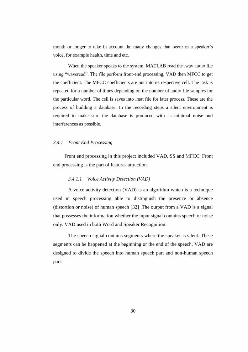
10),()()( Nnnwnxny ll .Typically the Hamming window is used,
which has the form: 10,1
2cos46.054.0)(
Nn
N
nnw
as shown
in Figure 16.
40
Figure 16 256 points hamming window [36]
3.4.1.3.3 Fast Fourier Transform (FFT)
Fast Fourier Transform, which converts each frame of N samples from
the time domain into the frequency domain. The FFT is a fast algorithm to
implement the Discrete Fourier Transform (DFT), which is defined on the set
of N samples {xn}, as
1
0
/2 1,...,2,1,0,N
n
Nknj
nk NkexX
In general Xk‟s are complex numbers and we only consider their
absolute values (frequency magnitudes). The resulting sequence {Xk} is
interpreted as follow: positive frequencies 2/0 sFf correspond to values
12/0 Nn , while negative frequencies 02/ fFs correspond to
112/ NnN . Here, Fs denote the sampling frequency.

41
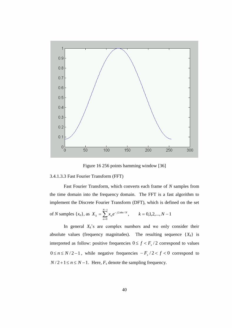
3.4.1.3.4 Mel-Frequency Wrapping
Mel-Frequency Wrapping maps frequency components using a Mel
scale modeled based on the human ear perception of sound instead of a linear
scale [36]. Filter bank is an approach to simulate the subjective spectrum which
it spaced uniformly on the mel-scale as shown at Figure 17. The mel-frequency
scale is linear frequency spacing below 1000 Hz and a logarithmic spacing
above 1000 Hz as shown in Figure 18. This is the scale where much similar to
the perception model of human ear. The Mel-frequency cepstrum represents the
short-term power spectrum of a sound using a linear cosine transform of the log
power spectrum of a Mel scale. The formula for the Mel scale is
which mean if a pitch of 1 kHz tone, 40 dB above the
perceptual hearing threshold, the value of mel is 1000 Mels. Mel filter bank is
best to view each filter as a histogram bin in frequency and the bins have
overlap.
Figure 17 Mel filter bank operating on a spectrum [36]
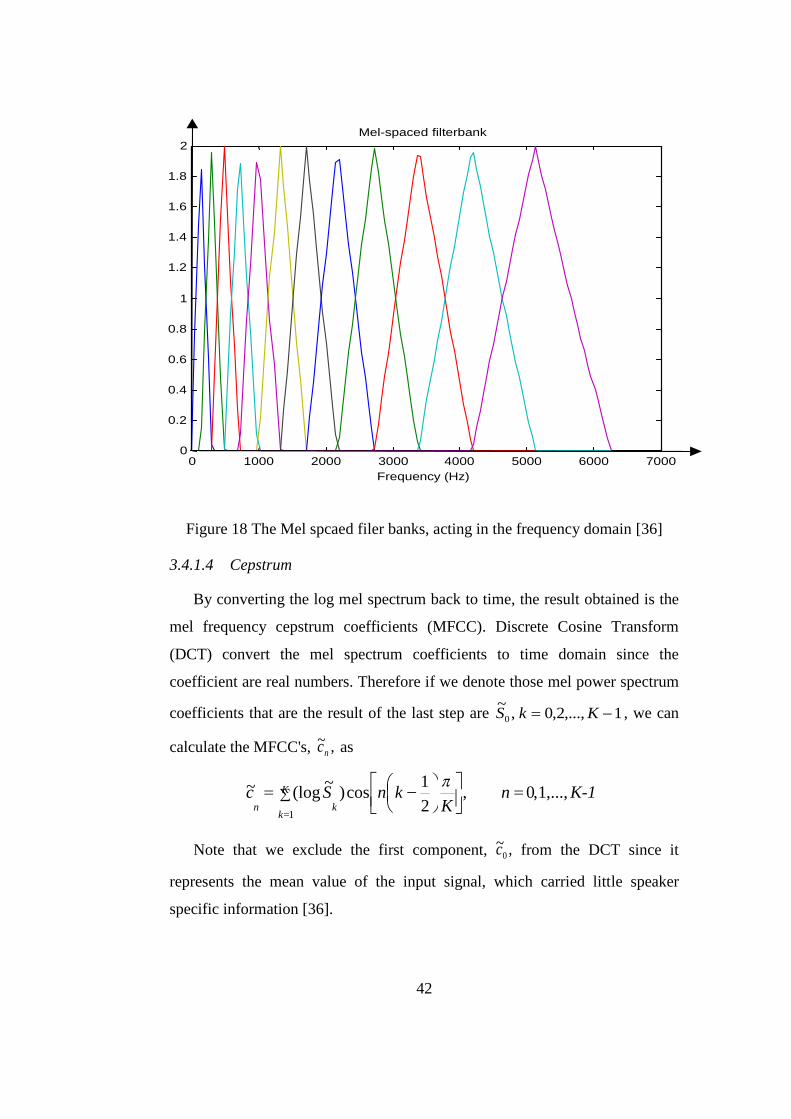
42
Figure 18 The Mel spcaed filer banks, acting in the frequency domain [36]
3.4.1.4 Cepstrum
By converting the log mel spectrum back to time, the result obtained is the
mel frequency cepstrum coefficients (MFCC). Discrete Cosine Transform
(DCT) convert the mel spectrum coefficients to time domain since the
coefficient are real numbers. Therefore if we denote those mel power spectrum
coefficients that are the result of the last step are 1,...,2,0,~
0 KkS , we can
calculate the MFCC's, ,~nc as
Note that we exclude the first component, ,~0c from the DCT since it
represents the mean value of the input signal, which carried little speaker
specific information [36].
K-1 n K
k n S c K
k k n
,..., 1 , 0 , 2
1 cos )
~ (log ~
1
0 1000 2000 3000 4000 5000 6000 70000
0.2
0.4
0.6
0.8
1
1.2
1.4
1.6
1.8
2
Mel-spaced filterbank
Frequency (Hz)

43
3.4.2 Word Recognition
Word Recognition identifies what the speaker said by referring to the
database.
3.4.2.1 Dynamic Time Warping (DTW)
Dynamic time warping (DTW) is a well-known method to find the best
alignment between two given (time-dependent) sequences with certain
restrictions. DTW has been used to compare different speech patterns in
automatic speech recognition. The speed when we are talking, every single
time there must be at least some different in speed. Some time we talk slower
when we are tired, some time we talk quicker when we get nervous and all
depends on the situation. DTW has earn its popularity by being extremely
efficient as the time-series similarity measure which minimizes the effect of
shifting and distortion in time by allowing “elastic” transformation of time
series in order to detect similar shapes with different phases [37]. Dynamic
time warping is a clever technique which lies in the computation of the distance
between input streams and templates. Algorithm is used to search the space of
mappings from the time sequence of the input stream to that of the template
stream, so that the total distance is minimize instead of comparing the value of
the input stream at time, t to the template stream at time, t as shown in Figure
19 [38].
Figure 19 Time Alignment of two time-dependent sequences [38]

44
For this project, there are two time series, one is MFCC coefficient T =
(t1, t2…., tN) of length N ϵ ℕ another one is the database coefficient R = (r1, r2….
rM) of length M ϵ ℕ. These sequences sampled at equidistant points in time and
fix a features space denoted by ƥ. Then tn, rm ϵ ƥ for n ϵ [1: N] and m ϵ [1 : M].
To compare t, r ϵ ƥ, local cost measure or local distance measure is used. The
function is localcost : ƥ x ƥ ℝ ≥ 0. In general, localcost is small if t and r are
similar to each other or else localcost is large.
Algorithm starts by building the distance matrix by using “repmat” in
MATLAB software which represent all pair wise distance between t and r. This
distance matrix called local cost matrix for alignment of two sequence t and r:
Cl ϵ ℝ M x N : Ci,j = || ti – rj || , i ϵ [1 : N] , j ϵ [1: M] [38].
Next, Optimal Warping Path which is a warping path that has a minimal
cost among all possible warping paths between T and R. To obtain the optimal
path, every possible warping between T and R need to be tested which causing
computational complexity that is exponential in the lengths T and R. To handle
this problem, Dynamic Programming does the job. The total cost of function is
Cp( T, R ) = . The DTW function is DTW(T,R) = Cp*( T, R )
= min{Cp( T, R ), p ϵ PN x M
}where PN x M
is the set of all possible warping paths.
The accumulated cost matrix D are defined as follows: 1. D( 1, j ) =
C(t1,rk) , j ϵ [1:M] ; 2. D( i, 1) =
C(tk,r1), i ϵ [1:N] ; 3. D( i, j ) =
min{D( i – 1, j – 1), D( i – 1, j ), D( i, j – 1)} + C( ti, rj ), I ϵ [1,N] , j[1:M]. [37]
As a conclusion, DTW is first figure out the difference of the two time
series by building the accumulated cost matrix then finding the optimal
warping path to get all the value for every single pair between T and R [38].

45
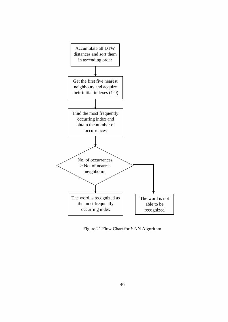
3.4.2.2 k-Nearest Neighbour
In pattern recognition, the k-nearest neighbour algorithm (k-NN) is a
method for classifying objects based on closest training. In the project, the
result obtained in the Dynamic Time Warping algorithm will be sorted
accordingly in k-NN algorithm. k-nearest neighbour algorithm works based on
minimum distance from the query instance to the training samples to determine
the k-nearest neighbours. After gather k-nearest neighbours, we take simple
majority of these k-nearest neighbors to be the prediction of the query instance.
Figure 20 k-NN classifications
Example of k-NN classifications by referring to Figure 20. The test
sample which is the diamond shape should be classified either to the first class
of pentagon or to the second class of stars. If k = 3, it is classified to the second
class because there are 2 stars and only 1 pentagon inside the inner circle. If k
= 5 it is classified to first class, 3 pentagon vs. 2 stars inside the outer circle
[39]. Figure 21 shows the flow chart of the k-NN algorithm.
46
Figure 21 Flow Chart for k-NN Algorithm
Accumulate all DTW
distances and sort them
in ascending order
Get the first five nearest
neighbours and acquire
their initial indexes (1-9)
Find the most frequently
occurring index and
obtain the number of
occurrences
The word is recognized as
the most frequently
occurring index
No. of occurrences
> No. of nearest
neighbours
The word is not
able to be
recognized

47
3.4.3 Speaker Recognition
Speaker Recognition is able to recognize who is the speaker from the
codebook.
3.4.3.1 Vector Quantization (VQ)
Vector Quantization is a technique used to compress the classification
and manipulate the data in a way to maintain the most prominent characteristic.
VQ can also be called as a process of mapping vectors. From a large vector
space it map to a finite number of regions in that space. This finite region is
called a cluster. It can represent by its center called a codeword. Each
codeword is used to construct a codebook, this process is applied to every
single speaker to be trained into the system.
Linde-Buzo-Gray [40] or LBG VQ algorithm is implemented in this
project. The overflow of the algorithm is shown in Figure 22.

48
Figure 22 Flow Diagram of VQ-LBG Algorithm [41]
The LBG is using splitting method to obtain the codebook. LBG splits
the codebook into segments and performs a comprehensive analysis on each
segment. The analysis compresses the training vector information creating a
new codebook which is then used to compute the next segment [40].
According to Fuzzy Clustering, to start a splitting method, an initial
codevector is set as average, then split in two vectors. Then the two vectors are
run in the iterative algorithm. The results from these two vectors are further
Find
centroid
m=2*m
Cluster
Vectors
Split each
centroid
Find code
vectors
Compute D
(Distortion)
D‟ = D
Stop
No Yes
Yes

49
split into 2 vectors each become four vectors. This process is repeated until the
desired number of code vectors is obtained.
The process is proceeding continuously until all segments have been
processed and the new codebook is created. This process is to minimize any
distortions in the data creating a codebook which is computationally optimized,
while providing a sub-optimal solution.
The performance of VQ analysis is highly dependent on the length of
the voice file which is operated upon.
The algorithm makes the decision base on two of the criteria. First is,
the Euclidean Distance between the codebook tested and the trained codebooks.
Second is, the distance calculated falls below a pre-defined threshold of
acceptance. If the system could not met the threshold of this two requirement,
the voice signal in the test is will be shown “unknown speaker” [41].
Basically, the Speaker Recognition is run as shown in the block
diagram in Figure 23 and Figure 24.

50
Figure 23 Overview of Speaker Recognition Algorithm (Part 1)
Matlab waveread function imports
*.wav file into workspace
mfcc.m is executed on current
*.wav file
Vqlbg.m is executed using
computed mfcc as input
Compare k-NN using disteu.m
Find Centroids
Create codebook array
A

51
Figure 24 Overview of Speaker Recognition Algorithm (Part 2)
Matlab waveread function
imports *.wav file into
workspace
mfcc.m is executed on current
*.wav file
Compure k-NN using disteu.m
Find minimum distance
between test signal and trained
signal
A
If
Distance <
Threshold
“Test Speaker is Speaker n”
“Test Speaker is an
unknown Speaker”
Yes
No
52
3.5 Conclusion
Basically, to start work on this project two set of database need to be
recorded: Train and Test folder. When recording the database, a very silent
environment is required because a quality of a database affects the accuracy of
the system. There are many others way to work on the Word and Speaker
Recognition System. In this project VAD, SS and MFCC are used in front-end
processing. For back-end processing, DTW, k-NN and VQ are used.
53
Chapter 4
RESULT AND DISCUSSION
Word and Speaker recognition are inherent of a database, which stores
information used to compare the test word and speaker against a set of trained
words and speakers‟ voices. Ideally, storing as much database is advised
because it can give higher accuracy, but realistically this cannot be achieved. It
would be unfeasible and impractical to stores a number of feature vectors as it
require a very large storing place.
There are 10 people‟s voices utter words: “One”, “Two”, “Three”,
“Four”, “Five”, “Six”, “Seven”, “Eight” and “Nine” which are 5 female and 5
male.
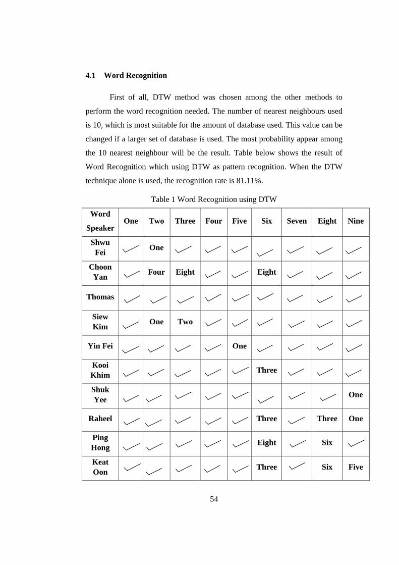
54
4.1 Word Recognition
First of all, DTW method was chosen among the other methods to
perform the word recognition needed. The number of nearest neighbours used
is 10, which is most suitable for the amount of database used. This value can be
changed if a larger set of database is used. The most probability appear among
the 10 nearest neighbour will be the result. Table below shows the result of
Word Recognition which using DTW as pattern recognition. When the DTW
technique alone is used, the recognition rate is 81.11%.
Table 1 Word Recognition using DTW
Word
Speaker One Two Three Four Five Six Seven Eight Nine
Shwu
Fei One
Choon
Yan
Four Eight Eight
Thomas
Siew
Kim
One Two
Yin Fei
One
Kooi
Khim
Three
Shuk
Yee
One
Raheel Three Three One
Ping
Hong
Eight Six
Keat
Oon Three Six Five
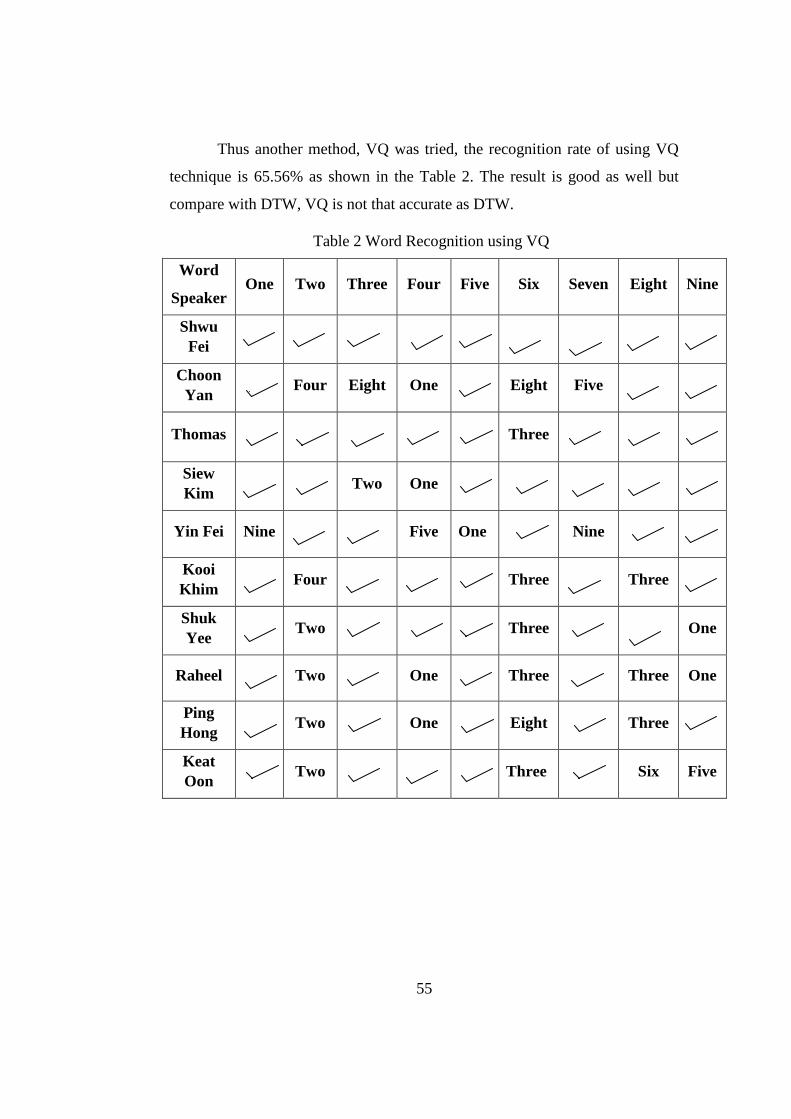
55
Thus another method, VQ was tried, the recognition rate of using VQ
technique is 65.56% as shown in the Table 2. The result is good as well but
compare with DTW, VQ is not that accurate as DTW.
Table 2 Word Recognition using VQ
Word
Speaker One Two Three Four Five Six Seven Eight Nine
Shwu
Fei
Choon
Yan
Four Eight One Eight Five
Thomas
Three
Siew
Kim Two One
Yin Fei Nine
Five One Nine
Kooi
Khim
Four Three Three
Shuk
Yee Two
Three
One
Raheel Two One Three Three One
Ping
Hong Two One Eight Three
Keat
Oon Two Three Six Five

56
To improve the recognition rate, both DTW and VQ are combined.
Obviously, the recognition rate is higher compare to previous result which is
84.44% as shown in the Table 3.
Table 3 Word Recognition using DTW and VQ
Word
Speaker One Two Three Four Five Six Seven Eight Nine
Shwu
Fei
Choon
Yan
Four Eight
Thomas
Siew
Kim
Two One
Yin Fei
One
Kooi
Khim
Four Three
Shuk
Yee
One
Raheel One
Ping
Hong
Eight Six
Keat
Oon Eight One Five

57
4.2 Speaker Recognition
For Speaker recognition, let‟s assume: Shwu Fei – SF ,Choon Yan –
CY, Thomas – T, Siew Kim – SY, Yin Fei – YF, Kooi Khim – KK, Shuk Yee
– SY, Raheel – R, Ping Hong – PH and Keat Oon -- KO
At first DTW method was chosen but the accuracy is low which is
35.56% as shown in Table 3.
Table 4 Speaker Recognition using DTW
Word
Speaker One Two Three Four Five Six Seven Eight Nine
Shwu
Fei
CY YF
Choon
Yan SF PH SF SK PH SF
Thomas KK PH PH SK SF PH KK PH
Siew
Kim
PH PH SF PH KO
Yin Fei SK SK SK CY CH
Kooi
Khim SK PH YF PH SF YF YF YF YF
Shuk
Yee PH PH SF PH PH YF
Raheel PH PH PH PH PH PH SF PH SK
Ping
Hong SK SF
Keat
Oon PH PH PH SF SF

58
Due to the accuracy is not that high, another method was used which is
VQ method was chosen for the speaker recognition purpose. The accuracy for
Speaker Recognition that using VQ method has the recognition rate slightly
higher than DTW method which is 42.22%.
Table 5 Speaker Recognition using VQ
Word
Speaker One Two Three Four Five Six Seven Eight Nine
Shwu
Fei CY CY
Choon
Yan YF SF SF SF YF YF YF
Thomas PH KO KK YF PH PH
Siew
Kim
PH SF T YF
Yin Fei SK SK SK CY CY
Kooi
Khim YF PH PH SF YF YF
Shuk
Yee SK PH PH SF PH SK PH YF
Raheel PH KO PH CY PH SK
Ping
Hong YF KK SF
Keat
Oon KK T T PH KK
Due to the low recognition rate of speaker recognition, the high
accuracy of word recognition is make used to improve the speaker recognition
rate.
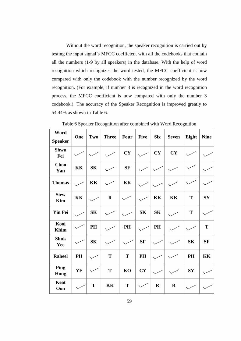
59
Without the word recognition, the speaker recognition is carried out by
testing the input signal‟s MFCC coefficient with all the codebooks that contain
all the numbers (1-9 by all speakers) in the database. With the help of word
recognition which recognizes the word tested, the MFCC coefficient is now
compared with only the codebook with the number recognized by the word
recognition. (For example, if number 3 is recognized in the word recognition
process, the MFCC coefficient is now compared with only the number 3
codebook.). The accuracy of the Speaker Recognition is improved greatly to
54.44% as shown in Table 6.
Table 6 Speaker Recognition after combined with Word Recognition
Word
Speaker One Two Three Four Five Six Seven Eight Nine
Shwu
Fei CY CY CY
Choo
Yan KK SK SF
Thomas KK KK
Siew
Kim KK R KK KK T SY
Yin Fei SK SK SK T
Kooi
Khim
PH PH PH T
Shuk
Yee SK SF SK SF
Raheel PH T T PH
PH KK
Ping
Hong YF T KO CY SY
Keat
Oon T KK T R R
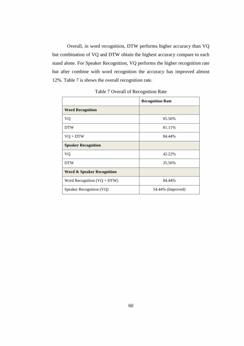
60
Overall, in word recognition, DTW performs higher accuracy than VQ
but combination of VQ and DTW obtain the highest accuracy compare to each
stand alone. For Speaker Recognition, VQ performs the higher recognition rate
but after combine with word recognition the accuracy has improved almost
12%. Table 7 is shows the overall recognition rate.
Table 7 Overall of Recognition Rate
Recognition Rate
Word Recognition
VQ 65.56%
DTW 81.11%
VQ + DTW 84.44%
Speaker Recognition
VQ 42.22%
DTW 35.56%
Word & Speaker Recognition
Word Recognition (VQ + DTW) 84.44%
Speaker Recognition (VQ) 54.44% (Improved)

61
4.3 Miscellaneous
When recording the database, a few steps need to be taken. The voices
utter to the speaker must not exceed the threshold 1. Figure 25 shows the
voices over the limit while Figure 26 shows the correct volume of the voices.
Figure 25 Database over the volume limit

62
Figure 26 Database within the volume limit

63
Figure 27-31 show the differences of the waveform when the voices
pass through every algorithm. The waveform shown is from Speaker Shwu Fei.
Figure 27 is the original waveform of word “One”.
Figure 27 Original waveform for word "One"

64
Figure 28 shows the waveform after the VAD which is the step to
differentiate the human speech and non human speech.
Figure 28 Waveform after VAD

65
Figure 29 shows the waveform after SS which is used to eliminate the
noise.
Figure 29 Waveform after SS
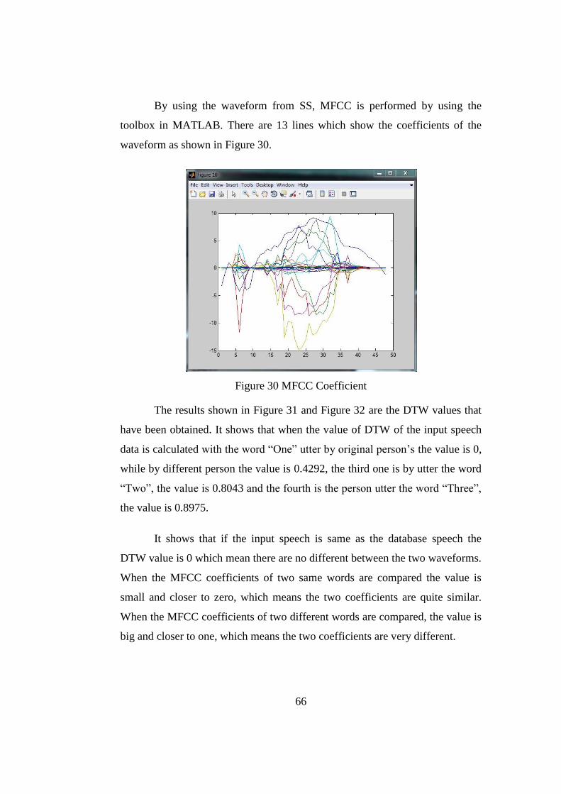
66
By using the waveform from SS, MFCC is performed by using the
toolbox in MATLAB. There are 13 lines which show the coefficients of the
waveform as shown in Figure 30.
Figure 30 MFCC Coefficient
The results shown in Figure 31 and Figure 32 are the DTW values that
have been obtained. It shows that when the value of DTW of the input speech
data is calculated with the word “One” utter by original person‟s the value is 0,
while by different person the value is 0.4292, the third one is by utter the word
“Two”, the value is 0.8043 and the fourth is the person utter the word “Three”,
the value is 0.8975.
It shows that if the input speech is same as the database speech the
DTW value is 0 which mean there are no different between the two waveforms.
When the MFCC coefficients of two same words are compared the value is
small and closer to zero, which means the two coefficients are quite similar.
When the MFCC coefficients of two different words are compared, the value is
big and closer to one, which means the two coefficients are very different.

67
Figure 31 MFCC coefficient of the input speech
Figure 32 Test words for One by original speech, One by different person,
Two, Three (From left to right)
DTW Distance
= 0
DTW Distance
= 0.4249
DTW Distance
= 0.8043
DTW Distance
= 0.8975

68
4.4 Conclusion
When doing the testing, the microphone used could not perform well.
To improve the performance, a better quality of microphone must be used so
that the words utter by the speaker can be captured accurately and the result
might be more accurate. When recording the database, the environment must
be silent enough to reach the most accuracy. A complete word recognition
system and speaker recognition system are successfully built with recognition
rate of 84.44 % for word recognition and 54.44% for speaker recognition.

69
Chapter 5
CONCLUSION AND RECOMMENDATIONS
As a conclusion, the methods used in word and speaker recognition
system are being explored. This project involves two main parts: Speech/Word
Recognition and Speaker Recognition. The main tool for this project is
MATLAB. Training and Testing are the important stages to perform. With
accurate training and testing stage the result will be more accurate.
5.1 Conclusion
The GOLD medal is achieved in Engineering Design Exhibition for this
project in Universiti Teknologi PETRONAS as shown in Appendix C while the
conference paper is accepted in 2011 International Conference on Software
Technology and Engineering (ICSTE 2011) as attach at Appendix D.
From the research, among so many methods to implement on the word
recognition, VAD, SS, MFCC, DTW, VQ and k-NN are used. MFCC is the
most popular method in pattern recognition. For speaker recognition, VQ is
used. A complete word recognition system and speaker recognition system are
successfully built with recognition rate of 84.44% for word recognition and
54.44% for speaker recognition.

70
The advantage of the project is focused on the improvement in security
provided by this Word and Speaker Recognition System. It can also be used by
the disable people. For example in the lift, they can utter the number of the
level they would like to reach instead of pressing the button of the lift which is
hard to reach by them.
5.2 Recommendation
The main idea of this project is to help the disable people to go to the
desired level they wish to go in the lift. With the combination of word and
speaker recognition, the lift not just needs to recognize the word utter by the
speaker but also must able to recognize who are the speakers. This will
improve the security of the building.
This project can be used together with PIC or Digital Signal Processing
development kits then it can be further used in the real world.
Last, the recognition rate can be improved by recording the database in
a very ideal environment. The quality of the database affects the accuracy of
the recognition rate.
71
REFERENCES
[1] M. R.Schroeder, “ Computer Speech Technology”. Second Edition,
Boston New York, 1999.pp 41-45
[2] R.D. Peacocke, “An Introduction to Speech and Speaker Recognition”,
IEEE Press, Bell Northern Research, 1990. pp26-33
[3] Fu, C, “An independent Workstation for a Quadriplegic”, In
International Excahnge of Experts and Informatiopn in Rehabilitation,
Monograph #37, Foulds, R. (ed.), World Rehabilitation Fund, New
York, 1986, pp.42-22.
[4] Salisbury, M.W., J.H.Hendrickson, T.L.Lammers, C.Fu, and
S.A.Moody, “Talk and Draw: Bundling Speech and Graphic,” IEEE
Computer, Vol. 23, No. 8, 1990, pp. 59-65.
[5] R. D. Rodman, “Computer Speech Technology”, Boston, London, 1999,
pp 272- 275.
[6] D. A. Reynolds, “An Overview of Automatic Speaker Recognition
Technology”, MIT Lincoln Laboratory, Lexington, MA USA, IEEE
2002 Vol. IV pp 4072-4075.
[7] T.W. Keong, “Speaker Recognition” [Online]. Available:
sst.unisim.edu.sg:8080/dspace/.../314/.../09_Thang%20Wee%20Keong.
doc [Accessed: Sept. 13, 2010]
[8] J. R. Deller, J. H.L. Hansen, J. G. Proakis, “Discrete-Time Processing
of Speech Signals”, IEEE Press, New York, NY, 2000. [Accessed:
Sept. 13, 2010]

72
[9] “An Automatic Speaker Recognition System” [Online]. Available:
http://www.ifp.uiuc.edu/~minhdo/teaching/speaker_recognition
[Accessed: Sept. 13, 2010]
[10] H. F. Olson and H. Belar, “Phonetic typewriter,” J.A.S.A., 28 (6), pp.
1072-1081, 1956.
[11] D. B. Fry, “Theoretical aspects of mechanical speech recognition”; and
P. Denes, “The design and operation of the mechanical speech
recognizer at University College London,” J. British Inst. Radio Engr.,
19, 4, pp. 211-229, 1959.
[12] J. W. Forgie and C. D. Forgie, “Results obtained from a vowel
recognition computer program,” J.A.S.A., 31 (11), pp. 1480-1489.
1959.
[13] T. K. Vintsyuk, “Speech discrimination by dynamic programming,”
Kibernetika, 4 (2), pp. 81- 88, 1968.
[14] D. R. Reddy, “An approach to computer speech recognition by direct
analysis of the speech wave,” Tech. Report No. C549, Computer
Science Dept., Stanford Univ., 1966.
[15] T. B. Martin, et. al., “Speech recognition by feature abstraction
techniques,” Tech. Report ALTDR- 64-176, Air Force Avionics Lab,
1964.
[16] K. Nagata, et. al., “Spoken digit recognizer for Japanese language,”
NEC Res. Develop., 6, 1963.
[17] L. R. Rabiner, et. al., “Speaker independent recognition of isolated
words using clustering techniques,” IEEE Trans. Acoustics, Speech,
Signal Proc., ASSP-27, pp. 336-349, 1979.
73
[18] B. Lowerre, “The HARPY speech understanding system,” Trends in
Speech Recognition, W. Lea, Ed., Speech Science Pub., pp. 576-586,
1990.
[19] J. Ferguson, Ed., Hidden Markov models for speech, IDA, Princeton,
NJ, 1980.
[20] S. Katagiri, “Speech pattern recognition using neural networks,” W.
Chou and B.-H. Juang (Eds.) Pattern Recognition in Speech and
Language Processing, CRC Press, pp. 115-147, 2003.
[21] B.-H. Juang and S. Furui, “Automatic speech recognition and
understanding: A first step toward natural human-machine
communication,” Proc. IEEE, 88, 8, pp. 1142-1165, 2000.
[22] C. H. Lee, “Statistical confidence measures and their applications,”
Proc. ICSP, pp. 1021-1028, 2001
[23] G. R. Doddington, “A method of speaker verification,” J.A.S.A., 49,
139 (A), 1971
[24] S. Pruzansky, “Pattern-matching procedure for automatic talker
recognition,” J.A.S.A., 35, pp. 354-358, 1963.
[25] S. Furui, “Cepstral analysis technique for automatic speaker
verification,” IEEE Trans. Acoustics, Speech, Signal Processing,
ASSP-29, pp. 254- 272, 1981.
[26] T. Matsui and S. Furui, “Comparison of text independent speaker
recognition methods using VQ-distortion and discrete/continuous
HMMs,” Proc. ICSLP, pp. II-157-160, 1992.
[27] T. Matsui and S. Furui, “Concatenated phoneme models for text-
variable speaker recognition,” Proc. ICASSP, pp. II-391-394, 1993
74
[28] Reynolds, D.A. and Heck, L.P., “Automatic Speaker Recognition:
Recent Progress, Current Applications and Future Trends,” American
Association for the Advancement of Science (AAAS) Symposium,
February 2000.
[29] M Abd-AlRahman ,” Chapter 3 Literature Review”. [Online].
Available:
http://dspace.fsktm.um.edu.my/bitstream/1812/111/5/Chapter%203.pdf.
[Accessed: Oct, 3 2010]
[30] K.C. Huang, “Robust Speech Recognition in Noisy Environments,
National Centre University, Taiwan. May 30, 2003.
[31] M.M Ali, “ Introduction to MATLAB”, second edition, Johor Darul
Ta‟zim, Malaysia. Universiti Teknologi Malaysia, 2005.
[32] J.Staderman, “VOICE ACTIVITY DETECTION IN NOISY
ENVIRONMENTS”,[Online]. Available: perso.telecom
paristech.fr/~chollet/Biblio/Congres/Audio/.../page1851.pdf. [Accessed:
Oct, 3 2010]
[33] L.R. Rabiner and M.R. Sambur, “An Algorithm for Determining the
Endpointd of Isolated Utterances”, The Bell System Technical Journal,
February 1975, pp.297-331
[34] S. F. Boll, “Suppression of Acoustic Noise in Speech Using Spectral
Subtraction” in Proc. IEEE Int. Conf. on Acoustics, speech, and signal
processing, Apr. 1979, vol. 27 pp.113
[35] 0. Brigham, “The Fast Fourier Transform”. Englewood Cliffs, NJ:
Prentice-Hall, 1974.
75
[36] M.R. Hasan, Mustafa Jamil, Md. Golam Rabbani, Md. Saifur Rahman.
"Speaker Identification using Mel Frequency cepstral coefficients". 3rd
International Conference on Electrical & Computer Engineering ICECE
2004, 28-30 December 2004, Dhaka, Bangladesh
[37] P.Senin, “Dynamic Time Warping Algorithm Review”, Information
and Computer Science Department, University of Hawaii, USA,
December 2008. pp 3-9
[38] M.W. Kadous, “ Dynamic Time Warping”, [Online]. Available:
http://www.cse.unsw.edu.au/~waleed/phd/html/node38.html [Accessed:
Oct,9 2010]
[39] “K-nearest neighbour algorithm”, [Online]. Available:
http://en.wikipedia.org/wiki/K-nearest_neighbor_algorithm [Accessed:
Oct, 9 2010]
[40] By Minh N. Do , Digital Signal Processing Mini-Project: An Automatic
Speaker Recognition System. [Online]. Available:
http://lcavwww.epfl.ch/~minhdo/asr_project/ [Accessed: March, 23
2011]
[41] Sookpotharom, S. Manas "Codebook Design Algorithm for Classified
Vector Quantization" Bangkok University, Pathumtani, Thailand pp.
751-753, 2000

76
APPENDICES
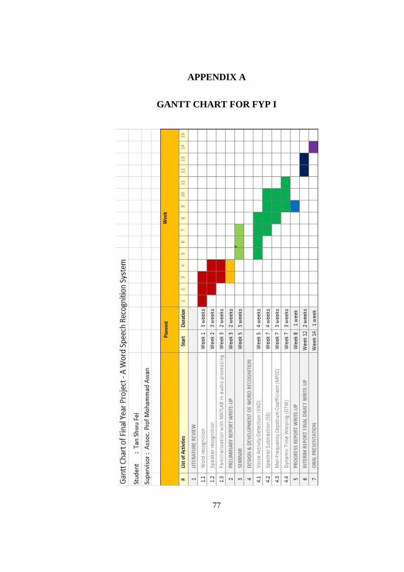
77
APPENDIX A
GANTT CHART FOR FYP I
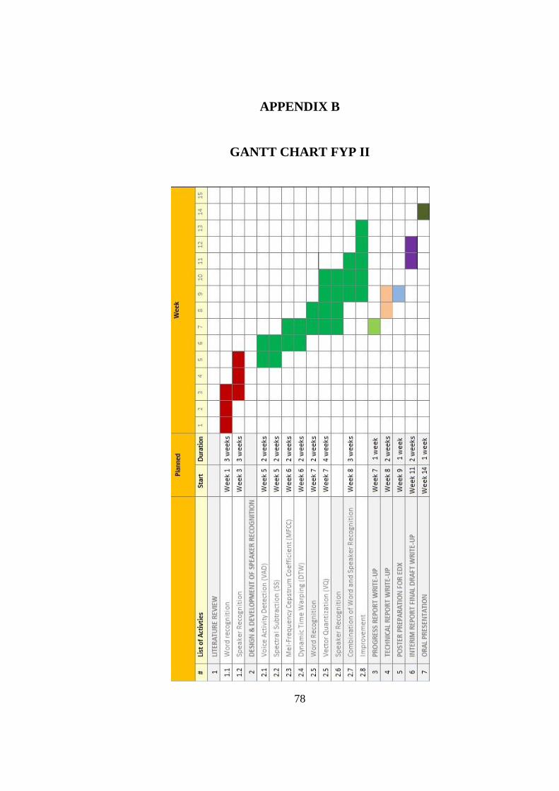
78
APPENDIX B
GANTT CHART FYP II

79
APPENDIX C
ENGINEERING DESIGN EXHIBITION

80

81
APPENDIX D
NOTIFICATION OF ACCEPTED PAPER BY ICSTE 2011

82

83

84
APPENDIX E
CONFERENCE PAPER