Markov Chain Models: Computations andApplicationsWai-Ki CHING

AMACL, Department of MathematicsThe University of Hong Kong

ICCM 2016, Beijing

Abstract: Markov chain models are popular mathematical tools forstudying many different kinds of real world systems such as queueingnetworks (continuous time) and categorical data sequences (discretetime). In this talk, I shall first present some efficient numerical algo-rithms for solving Markovian queueing networks. I shall then intro-duce some other parsimonious high-order and multivariate Markovchain models for categorical sequences with applications. Efficientestimation methods for solving the model parameters will also bediscussed. Practical problems and numerical examples will then begiven to demonstrate the effectiveness of our proposed models.

Research Supported in Part by HK RGC Grant Nos. HKU712602, 701707, and 17301214.

1

The Outline

(1) Motivations and Objectives.

(2) Queueing Systems.

(3) High-order Markov Chain Models.

(4) Multivariate Markov Chain Models.

(5) Concluding Remarks.

2

1. Motivations and Objectives.

• Markov chain models are popular tools for modeling many real

world systems including

• Continuous Time Markov Chain Process

-Queueing Systems.

-Telecommunication Networks.

-Manufacturing Systems.

-Re-manufacturing Systems.

• Discrete Time Markov Chain Process

-Categorical Time Series.

-Financial and Credit Risk Models.

-Genetic Networks and DNA Sequencing.

-Inventory Prediction and Control.

3

2. Queueing Systems

• [Queueing systems with Batch Arrival] R. Chan and W. Ching,

Toeplitz-circulant Preconditioners for Toeplitz Systems and Their

Applications to Queueing Networks with Batch Arrivals, SIAM Jour-

nal of Scientific Computing, 1996.

• [Manufacturing Systems with Production Control] W. Ching

et al., Circulant Preconditioners for Markov Modulated Poisson Pro-

cesses and Their Applications to Manufacturing Systems, SIAM

Journal on Matrix Analysis and Its Applications, 1997.

• [Queueing systems with Negative Customers] W. Ching, Itera-

tive Methods for Queuing Systems with Batch Arrivals and Negative

Customers, BIT, 2003.

• [Hybrid Method (Genetic Algorithm & SOR Iterative Method)]

W. Ching, A Hybrid Algorithm for Queueing Systems, CALCOLO,

2004.4

2.1.1 Single Markovian Queue (M/M/s/n-s-1)

• λ input rate (Arrival Rate),

• µ output rate (Service Rate, Production Rate).

• s number of servers.

• n− s− 1 number of waiting space.

• Set of possible states (number of customers): {0,1, . . . , n− 1}.

ss− 1

...

321

m��p pm��p pm��p p...

m��p pm��p pm��p p

1 2 3 · · · j · · · n− s− 1

p p p p p p · · · p p p p p p · · · λ�

�µ

�µ

�µ

�µ

�µ

�µ

: empty buffer in queue

p p : customer waiting in queuem��p p : customer being served

5

2.1.2 The Steady-state Distribution

• Let pi be the steady-state probability that i customers in thequeueing system and p = (p0, . . . , pn−1)

t be the steady-state prob-ability vector.

• Important for system performance analysis, e.g. average waitingtime of the customers in long run.

• B. Bunday, Introduction to Queueing Theory, Arnold, N.Y., 1996.

• pi governed by the Kolmogorov equations:

Out Going Rate Incoming Rate

� - - �pi−1 pi pi+1λ

iµpi−1 pi pi+1

(i+1)µ

λ

6

�

-

µ

���0

�

-

2µ

λ����1 · · · �

-

sµ

λ����s · · · ��

��n-1

�

-

sµ

λ

The Markov Chain of the M/M/s/n-s-1 Queue

• We are solving: A0p0 = 0,∑

pi = 1,pi ≥ 0.

• A0, the generator matrix, is given by the n×n tridiagonal matrix:

A0 =

λ −µ−λ λ+ µ −2µ 0

−λ λ+2µ −3µ· · ·

−λ λ+ sµ −sµ· · ·

0 −λ λ+ sµ −sµ−λ sµ

.

7

2.1.3 The Two-Queue Free Models

s1

s1 − 1

...

321

m��p pm��p pm��p p...

m��p pm��p pm��p p

1 2 3 · · · j · · · n1 − s1 − 1

p p p p p p · · · p p p p p p · · · λ1�

�µ1

�µ1

�µ1

�µ1

�µ1

�µ1

s2

s2 − 1

...

321

m��p pm��p pm��p p...

m��p pm��p pm��p p

1 2 3 · · · k · · · n2 − s2 − 1

p p p p p p · · · p p · · · � λ2

�µ2

�µ2

�µ2

�µ2

�µ2

�µ2

: empty buffer in queue

p p : customer waiting in queuem��p p : customer being served

8

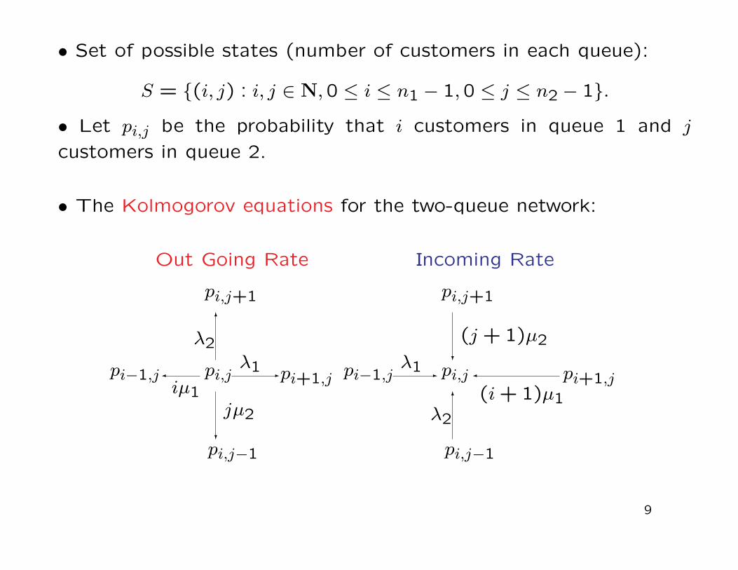
• Set of possible states (number of customers in each queue):

S = {(i, j) : i, j ∈ N,0 ≤ i ≤ n1 − 1,0 ≤ j ≤ n2 − 1}.

• Let pi,j be the probability that i customers in queue 1 and j

customers in queue 2.

• The Kolmogorov equations for the two-queue network:

Out Going Rate Incoming Rate

� -

?

6

- �

6

?

pi,j+1

pi,j−1

pi−1,j pi,j pi+1,j

jµ2

λ2λ1

iµ1

pi,j+1

pi,j−1

pi−1,j pi,j pi+1,j

λ2

(j +1)µ2

(i+1)µ1

λ1

9

• Again we have to solve A1p = 0,∑pij = 1,

pij ≥ 0.

• The generator matrix A1 is separable (no interaction between the

queues): A1 = A0 ⊗ I + I ⊗A0.

• Kronecker tensor product of two matrices Cn×r and Bm×k:

Cn×r ⊗Bm×k =

c11B · · · · · · c1rBc21B · · · · · · c2rB

... ... ... ...cn1B · · · · · · cnrB

nm×rk

.

• It is easy to check that the Markov chain of the queueing system

is irreducible and the unique solution is p = p0 ⊗ p0.

10

2.1.4 2-Queue Overflow Networks

s1

s1 − 1

...

321

m��p pm��p pm��p p...

m��p pm��p pm��p p

1 2 3 · · · j · · · n1 − s1 − 1

p p p p p p · · · p p p p p p p p · · · p p λ1�

��6

�µ1

�µ1

�µ1

�µ1

�µ1

�µ1

s2

s2 − 1

...

321

m��p pm��p pm��p p...

m��p pm��p pm��p p

1 2 3 · · · k · · · n2 − s2 − 1

p p p p p p · · · p p · · · � λ2

�µ2

�µ2

�µ2

�µ2

�µ2

�µ2

: empty buffer in queue

p p : customer waiting in queuem��p p : customer being served

• L. Kaufman, Matrix Methods for Queuing Problems, SIAM J. Sci. Statist. Comput., 1983.

11

• The generator matrix A2 is given by

A2 = A0 ⊗ I + I ⊗A0 +

(0

1

)⊗R0,

where

R0 = λ1

1−1 1 0

· ·· ·

0 −1 1−1 0

describes the overflow discipline of the queueing system.

• In fact, we may write

A2 = A1 +

(0

1

)⊗R0,

• Unfortunately analytic solution for the steady-state distributionp is not available.

12

• The generator matrices are sparse and have block structures.

• Direct method (LU decomposition will result in dense matrices L

and U) is not efficient in general.

• Fast algorithm should make use of the block structures and the

sparsity of the generator matrices.

• Block Gauss-Seidel (BGS) is an usual approach for mentioned

queueing problems. Its convergence rate is not fast and increase

linearly with respect to the size of the generator matrix in general.

• R. Varga, Matrix Iterative Analysis, Prentice-Hall, N.J., 1963.

13

2.2 The Telecommunication System

�

µ1

����s1 Queue 1

�λ1

@@@

@@R•••

�

µn

����sn Queue n �

λn

���

���

-λ Main Queue ����s -

µ

Size N

• W. Ching, Iterative Methods for Queuing and Manufacturing System, SpringerMonograph, 2001.

• W. Ching et al., Circulant Preconditioners for Markov Modulated Poisson Pro-

cesses and Their Applications to Manufacturing Systems, SIAM Journal on Matrix

Analysis and Its Applications, 1997.

14

• The generator matrix is given by:

A3 =

Q+Γ −µI 0−Γ Q+Γ+ µI −2µI

. . . . . . . . .−Γ Q+Γ+ sµI −sµI. . . . . . . . .

−Γ Q+Γ+ sµI −sµI0 −Γ Q+ sµI

,

((N +1)-block by (N +1)-block), where

Γ = Λ+ λI2n,

Q = (Q1⊗I2⊗· · ·⊗I2)+(I2⊗Q2⊗I2⊗· · ·⊗I2)+· · ·+(I2⊗· · ·⊗I2⊗Qn),

Λ = (Λ1⊗I2⊗· · ·⊗I2)+(I2⊗Λ2⊗I2⊗· · ·⊗I2)+· · ·+(I2⊗· · ·⊗I2⊗Λn),

Qj =

(σj1 −σj2−σj1 σj2

)and Λj =

(λj 00 0

).

15

2.3 The Manufacturing System of Two Machines in Tandem

M1 -

µ1

����B1

size l

- M2 -

µ2

����B2

size N

-

λ

• Search for optimal buffer sizes l and N (N >> l), which minimizes

(1) the average running cost, (2) maximizes the throughput, or (3)

minimizes the blocking and the starving rate.

• W. Ching, Iterative Methods for Manufacturing Systems of Two Stations inTandem, Applied Mathematics Letters, 1998.

• W. Ching, Markovian Approximation for Manufacturing Systems of Unreliable

Machines in Tandem, Naval Research Logistics, 2001.

16

The generator matrix is of the form:

A4 =

Λ+ µ1I −Σ 0−µ1I Λ+D + µ1I −Σ

... . . . . . .−µ1I Λ+D + µ1I −Σ

0 −µ1I Λ+D

,

((l+1)-block by (l+1)-block), where

Λ =

0 −λ 0

λ . . .. . . −λ

0 λ

, Σ =

0 0µ2

. . .

. . . . . .0 µ2 0

,

and

D = Diag(µ2, · · · , µ2,0).

17

2.4 The Re-Manufacturing System

-λ

Q?

-µ

N

ProcurementInventory

of Returns

-γ Inventory

of Product

Re-manu-

facturing· · ·

• There are two types of inventory to manage: the serviceable prod-uct and the returned product. The re-cycling process is modelledby an M/M/1/N queue.

• The product inventory level and outside procurements are con-trolled by an (Q, r) continuous review policy. Here r is the outsideprocurement level and Q is the procurement quantity. We assumethat N >> Q.

• W. Ching et al., An Inventory Model with Returns and Lateral Transshipments,Journal of the Operational Research Society, 2003.

• W. Ching et al., A Direct Method for Solving Block-Toeplitz with Near-

Circulant-Block Systems with Applications to Hybrid Manufacturing Systems,

Journal of Numerical Linear Algebra with Applications, 2005.

18

• The generator matrix is given by

A5 =

B −λI 0−L B −λI

. . . . . . . . .−L B −λI

−λI −L BQ

,

where

L =

0 µ 0

0 .. .. . . . . .

. . . µ0 0

, B = λIN+1 +

γ 0−γ γ + µ

. . . . . .. . . γ + µ

0 −γ µ

,

and

BQ = B −Diag(0, µ, . . . , µ).

19

2.5 Numerical Algorithm (Preconditioned Conjugate Gradi-

ent (PCG) Method)

• Conjugate Gradient (CG) Method to solve Ax = b.

• Need preconditioning to accelerate convergence rate.

• O. Axelsson, Iterative Solution Methods, Cambridge University

Press, 1996.

• In the Preconditioned Conjugate Gradient (PCG) method with

preconditioner C, CG method is applied to solve

C−1Ax = C−1b

instead of

Ax = b.

20

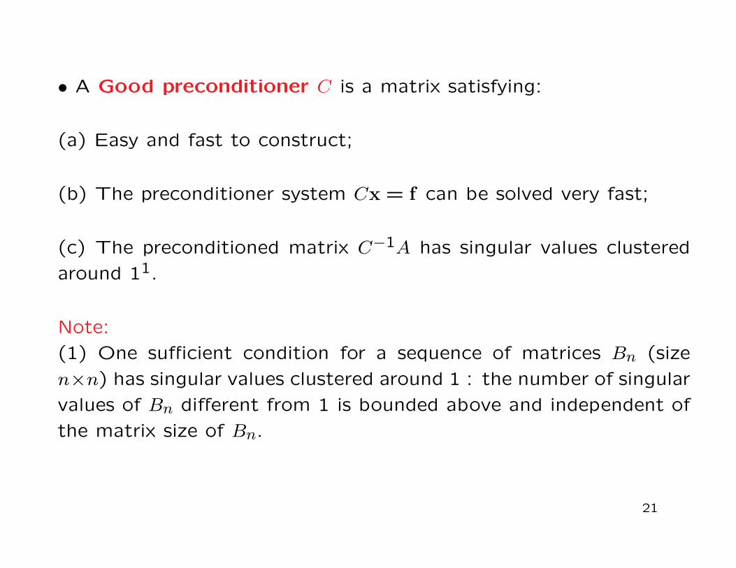
• A Good preconditioner C is a matrix satisfying:

(a) Easy and fast to construct;

(b) The preconditioner system Cx = f can be solved very fast;

(c) The preconditioned matrix C−1A has singular values clustered

around 11.

Note:

(1) One sufficient condition for a sequence of matrices Bn (size

n×n) has singular values clustered around 1 : the number of singular

values of Bn different from 1 is bounded above and independent of

the matrix size of Bn.

21

2.5.1 Circulant-based Preconditioners

• Circulant matrices are Toeplitz matrices (constant diagonal en-tries) such that each column is a cyclic shift of its preceding column.It is characterized by its first column.

• The class of circulant matrices is denoted by F.

− C ∈ F implies C can be diagonalized by Fourier matrix F :

C = F ∗ΛF.

Hence

C−1x = F ∗Λ−1Fx.

− Eigenvalues of a circulant matrix has analytic form, thereforeenhance the spectrum analysis of the preconditioned matrix.

− C−1x can be done in O(n logn).

• P. Davis, Circulant Matrices, John Wiley and Sons, N.J. 1985.

22

2.5.2 Circulant-based Preconditioner

The idea of circulant approximation:

A =

λ −µ 0−λ λ+ µ −2µ

· · ·−λ λ+ sµ −sµ

· · ·−λ λ+ sµ −sµ

0 −λ sµ

.

s(A) =

λ+ sµ −sµ −λ−λ λ+ sµ −sµ

· · ·−λ λ+ sµ −sµ

· · ·−λ λ+ sµ −sµ

−sµ −λ λ+ sµ

.

We have rank(A− s(A)) = s+1.

23

2.5.3 The Telecommunication System

•A3 = I ⊗Q+A⊗ I +R⊗ Λ, where

R =

1 0−1 1

−1 .. .. . . 1

0 −1 0

.

•s(A3) = s(I)⊗Q+ s(A)⊗ I + s(R)⊗ Λ, where

s(I) = I and s(R) =

1 −1−1 1

−1 .. .. . . 1

0 −1 1

.

24

2.5.4 The Manufacturing System of Two Machines in Tandem

• Circulant-based approximation of A4 : s(A4) =s(Λ) + µ1I −s(Σ) 0

−µ1I s(Λ) + s(D) + µ1I −s(Σ).. . . . . . . .

−µ1I s(Λ) + s(D) + µ1I −s(Σ)0 −µ1I s(Λ) + s(D)

,

((l+1)-block by (l+1)-block), where

s(Λ) =

λ −λ 0

λ . . .. . . −λ

−λ λ

, s(Σ) =

0 µ2µ2

. . .

. . . . . .0 µ2 0

,

and

s(D) = Diag(µ2, · · · , µ2, µ2).

25

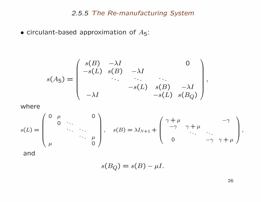
2.5.5 The Re-manufacturing System

• circulant-based approximation of A5:

s(A5) =

s(B) −λI 0−s(L) s(B) −λI

. . . . . . . . .−s(L) s(B) −λI

−λI −s(L) s(BQ)

,

where

s(L) =

0 µ 0

0 .. .. . . . . .

. . . µµ 0

, s(B) = λIN+1 +

γ + µ −γ−γ γ + µ

. . . . . .0 −γ γ + µ

,

and

s(BQ) = s(B)− µI.

26

2.5.6 Stochastic Automata Networks

• In fact, all the generator matrices A take the following form:

A =m∑

i=1

n⊗j=1

Aij,

where Ai1 is relatively huge in size.

• Our preconditioner is defined as

C =m∑

i=1

s(Ai1)n⊗

j=2

Aij.

• We note thatF n⊗j=2

I

∗CF n⊗

j=2

I

=m∑

i=1

Λi1

n⊗j=2

Aij =ℓ⊕

k=1

m∑i=1

λki1

n⊗j=2

Aij

which is a block-diagonal matrix.

27

• One of the advantages of our preconditioner is that it can be

inverted in parallel by using a parallel computer easily. This would

therefore save a lot of computational cost.

• Theorem: If all the parameters stay fixed then the preconditioned

matrix has singular values clustered around one. Thus we expect

our PCG method converges very fast.

• Ai1 ≈ Toeplitz except for rank (s+1) perturbation

≈ s(Ai1) except for rank (s+1) perturbation.

• R. Chan and W. Ching, Circulant Preconditioners for Stochastic

Automata Networks, Numerise Mathematik, (2000).

28

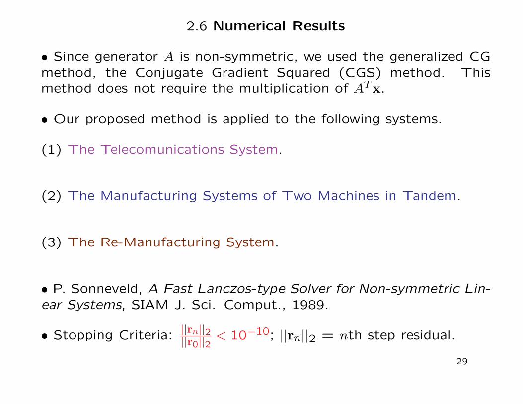
2.6 Numerical Results

• Since generator A is non-symmetric, we used the generalized CGmethod, the Conjugate Gradient Squared (CGS) method. Thismethod does not require the multiplication of ATx.

• Our proposed method is applied to the following systems.

(1) The Telecomunications System.

(2) The Manufacturing Systems of Two Machines in Tandem.

(3) The Re-Manufacturing System.

• P. Sonneveld, A Fast Lanczos-type Solver for Non-symmetric Lin-ear Systems, SIAM J. Sci. Comput., 1989.

• Stopping Criteria: ||rn||2||r0||2

< 10−10; ||rn||2 = nth step residual.

29

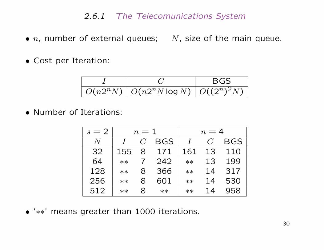
2.6.1 The Telecomunications System

• n, number of external queues; N , size of the main queue.

• Cost per Iteration:

I C BGSO(n2nN) O(n2nN logN) O((2n)2N)

• Number of Iterations:

s = 2 n = 1 n = 4N I C BGS I C BGS32 155 8 171 161 13 11064 ∗∗ 7 242 ∗∗ 13 199128 ∗∗ 8 366 ∗∗ 14 317256 ∗∗ 8 601 ∗∗ 14 530512 ∗∗ 8 ∗∗ ∗∗ 14 958

• ’∗∗’ means greater than 1000 iterations.

30

2.6.2 The Manufacturing Systems of Two Machines in Tandem

• l, size of the first buffer; N , size of the second buffer.

• Cost per Iteration:

I C BGSO(lN) O(lN logN) O(lN)

• Number of Iterations:

l = 1 l = 4N I C BGS I C BGS32 34 5 72 64 10 7264 129 7 142 139 11 142128 ∗∗ 8 345 ∗∗ 12 401256 ∗∗ 8 645 ∗∗ 12 ∗∗1024 ∗∗ 8 ∗∗ ∗∗ 12 ∗∗

• ’∗∗’ means greater than 1000 iterations.

31

2.6.3 The Re-Manufacturing System

• Q, size of the serviceable inventory; N , size of the return inventory.

• Cost per iteration:

I C BGSO(QN) O(QN logN) O(QN)

• Number of Iterations:

Q = 2 Q = 3 Q = 4N I C BGS I C BGS I C BGS100 246 8 870 ∗∗ 14 1153 ∗∗ 19 1997200 ∗∗ 10 1359 ∗∗ 14 ∗∗ ∗∗ 19 ∗∗400 ∗∗ 10 ∗∗ ∗∗ 14 ∗∗ ∗∗ 19 ∗∗800 ∗∗ 10 ∗∗ ∗∗ 14 ∗∗ ∗∗ 19 ∗∗

• ’∗∗’ means greater than 2000 iterations.

32

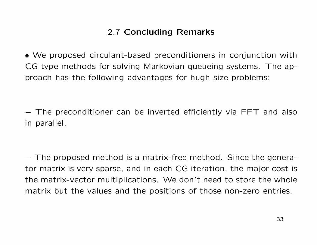
2.7 Concluding Remarks

• We proposed circulant-based preconditioners in conjunction with

CG type methods for solving Markovian queueing systems. The ap-

proach has the following advantages for hugh size problems:

− The preconditioner can be inverted efficiently via FFT and also

in parallel.

− The proposed method is a matrix-free method. Since the genera-

tor matrix is very sparse, and in each CG iteration, the major cost is

the matrix-vector multiplications. We don’t need to store the whole

matrix but the values and the positions of those non-zero entries.

33

3. High-order Markov Chain Models.

• Markov chains are popular models for solving many practical sys-

tems including categorical time series.

• It is also very easy to construct a Markov chain model. Given

the observed time series data sequence (Markov chain) {Xt} of m

states, one can count the transition frequency Fjk (one step) in

the observed sequence from State k to State j in one step.

• Hence one can construct the one-step transition frequency ma-

trix for the observed sequence {Xt} as follows:

F =

F11 · · · · · · F1mF21 · · · · · · F2m... ... ... ...

Fm1 · · · · · · Fmm

. (1)

34

• From F , one can get the estimates for Pkj (column normaliza-

tion) as follows:

P =

P11 · · · · · · P1mP21 · · · · · · P2m... ... ... ...

Pm1 · · · · · · Pmm

(2)

where

Pkj =Fkj

m∑r=1

Frj

is the maximum likelihood estimator.

35

• Example 1: Consider a data sequence of 3 states/categories:

{1,1,2,2,1,3,2,1,2,3,1,2,3,1,2,3,1,2,1,2}. (3)

We adopt the following notation. The sequence {Xt} can be writtenin vector form (canonical representation by Robert J. Elliott):

X0 = (1,0,0)T , X1 = (1,0,0)T , X2 = (0,1,0)T , . . . , X19 = (0,1,0)T .

• The First-order Markov Chain Model:By counting the transition frequency from State k to State j inthe sequence, one can construct the transition frequency matrix F

(then the transition probability matrix Q̂) for the sequence.

F =

1 3 36 1 11 3 0

and Q̂ =

1/8 3/7 3/46/8 1/7 1/41/8 3/7 0

(4)

and the first-order Markov chain model is

Xt+1 = Q̂Xt.

36

Robert J. Elliott (University of Calgary).

Hidden Markov models and financial engineering.

Ph.D. and Sc.D. (Cambridge University)

37

3.1 The Steady-state Probability Distribution

Proposition 3.1: Given an irreducible and aperiodic Markov chain

of m states, then for any initial probability distribution X0

limt→∞

||Xt − π|| = limt→∞

||P tX0 − π|| = 0.

where π is the steady-state probability distribution of the tran-

sition probability matrix P of the underlying Markov chain and

π = Pπ.

• We remark that a non-negative probability vector π satisfies π =

Pπ is called a stationary probability vector. A stationary proba-

bility vector is not necessary the steady-state probability distri-

bution vector.

38

Proposition 3.2: [Perron (1907) - Frobenius (1912) Theorem] Let

A be a non-negative, irreducible and aperiodic square matrix of

size m. Then

(i) A has a positive real eigenvalue λ, equal to its spectral radius,

λ = max1≤k≤m

|λk(A)|

where λk(A) denotes the kth eigenvalue of A.

(ii) There corresponds an eigenvector z, its entries being real and

positive, such that Az = λz.

(iii) The eigenvalue λ is a simple eigenvalue of A.

This theorem is important in Markov chains and dynamical systems.

39

• We remark that requirement aperiodic is important. The follow-

ing matrix is non-negative and irreducible but not aperiodic:

Q =

0 0 · · · 0 11 0 .. . 00 1 0 .. . ...... . . . . . . . . . 00 · · · 0 1 0

(5)

Now we see that all eigenvalues of Q are given by

λj = e2πij/n j = 0,1, . . . , n− 1

and they all satisfy |λj| = 1. They are all on the unit circle. We

see that π = (1,1, · · · ,1)T is the stationary probability vector but

it is not the steady-state distribution vector. In fact, begin with

x0 = (1,0,0, · · · ,0)T , xt does not converge to π. But we have

limn→∞

1

n

n∑i=1

xi = π.

40

Oskar Perron (7 May 1880 - 22 February 1975).

(Taken from Wikipedia, the free encyclopedia)

Differential equations and partial differential equations.

41

Ferdinand Georg Frobenius (October 26, 1849 - August 3, 1917).

(Taken from Wikipedia, the free encyclopedia)

Differential equations and group theory.

He gave the first full proof for the Cayley-Hamilton theorem.

42

3.2 Motivations for High-order Markov Chain Models.

• Categorical data sequences occur frequently in many real world

applications. The delay effects occur in many applications and data.

(i) Inventory Control and Demand Forecasting. W. Ching et al.,

A Higher-order Markov Model for the Newsboy’s Problem, Journal

of Operational Research Society, 54 (2003) 291-298.

(ii) Genetic Networks and DNA Sequencing. W. Ching et al.,

Higher-order Markov Chain Models for Categorical Data Sequences,

Naval Research Logistics, 51 (2004) 557-574.

(iii) Financial and Credit Risk Models. T. Siu, W. Ching et

al., A Higher-Order Markov-Switching Model for Risk Measurement,

Computers & Mathematics with Applications, 58 (2009) 1–10.

43

3.3 High-order Markov Chain Models.

• High-order Markov chain can better model categorical data se-quence (to capture the delay effect).

• Problem: A conventional n-th order Markov chain of m states hasO(mn) states and therefore parameters. The number of transitionprobabilities (to be estimated) increases exponentially with respectto the order n of the model.

(i) P. Jacobs and P. Lewis, Discrete Time Series Generated byMixtures I : Correlational and Runs Properties, J. R. Statist. Soc.B, 40 (1978) 94–105.

(ii) G. Pegram, An Autoregressive Model for Multilag Markov Chains,J. Appl. Prob., 17 (1980) 350–362.

(iii) A.E. Raftery, A Model for High-order Markov Chains, J. R.Statist. Soc. B, 47 (1985) 528–539.

44

Adrian E. Raftery, University of Washington.

Statistical methods for social, environmental and health sciences.

C. Clogg Award (1998) and P. Lazarsfeld Award (2003)

World’s most cited researcher in mathematics for the decade

1995-2005

45

• Raftery proposed a high-order Markov chain model which in-

volves only one additional parameter for each extra lag.

• The model:

P (Xt = k | Xt−1 = k1, . . . , Xt−n = kn) =n∑

i=1

λiqkki (6)

where k, k1, . . . , kn ∈ M . Here M = {1,2, . . . ,m} is the set of the

possible states and

n∑i=1

λi = 1 and Q = [qij]

is a transition probability matrix with column sums equal to one,

such that

0 ≤n∑

i=1

λiqkki ≤ 1, k, k1, . . . , kn = 1,2, . . . ,m. (7)

46

• Raftery proved that Model (6) is analogous to the standard

AR(n) model in time series.

• The parameters qk0ki, λi can be estimated numerically by maximiz-

ing the log-likelihood of Model (6) subjected to the constraints

(7).

• Problems:

(i) This approach involves solving a highly non-linear optimization

problem (which is not easy to solve).

(ii) The proposed numerical method neither guarantees convergence

nor a global maximum.

47

3.4 Our High-order Markov Chain Model.

• Raftery’s model can be generalized as follows:

Xt+n+1 =n∑

i=1

λiQiXt+n+1−i. (8)

• We define Qi to be the ith step transition probability matrix

of the sequence.

• We also assume that λi are non-negative such that

n∑i=1

λi = 1

so that the right-hand-side of Eq. (8) is a probability distribution.

48

3.5 A Property of the Model.

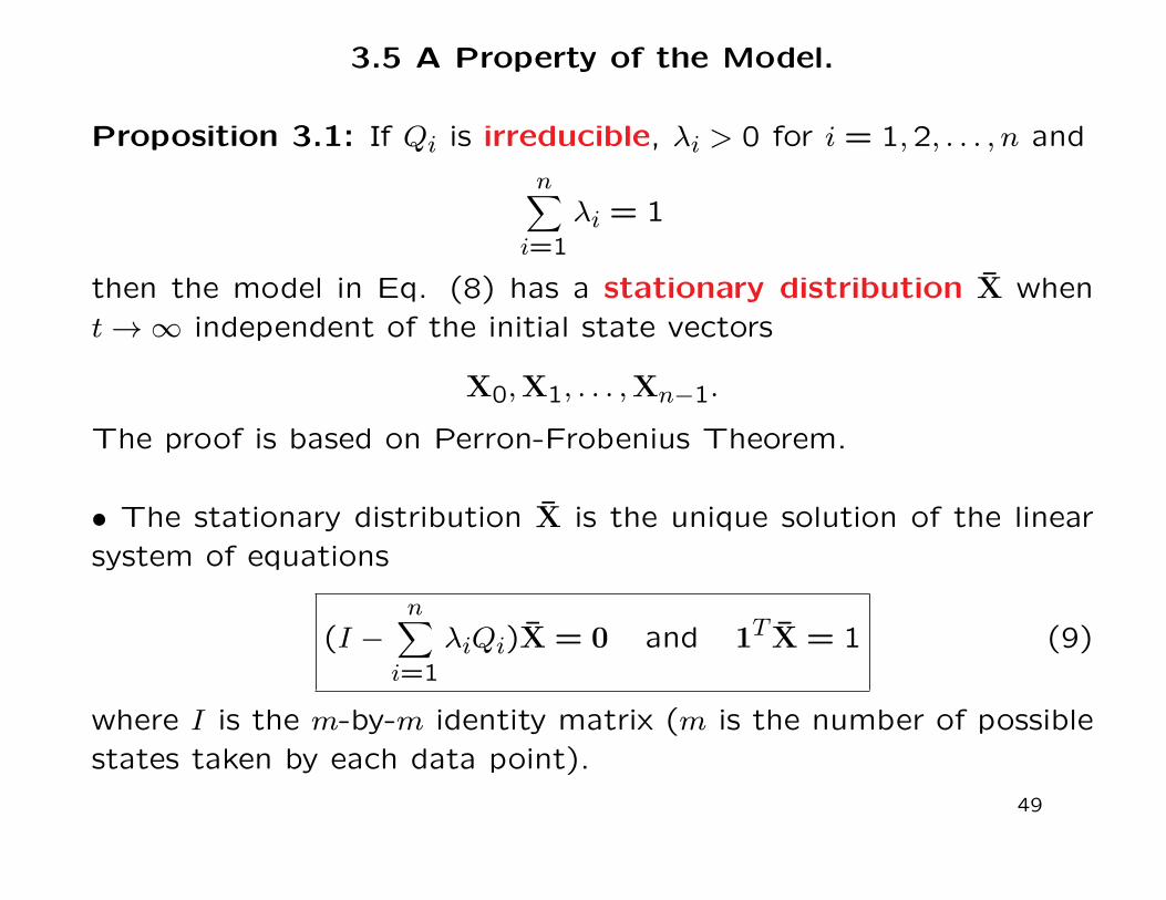
Proposition 3.1: If Qi is irreducible, λi > 0 for i = 1,2, . . . , n and

n∑i=1

λi = 1

then the model in Eq. (8) has a stationary distribution X̄ whent → ∞ independent of the initial state vectors

X0,X1, . . . ,Xn−1.

The proof is based on Perron-Frobenius Theorem.

• The stationary distribution X̄ is the unique solution of the linearsystem of equations

(I −n∑

i=1

λiQi)X̄ = 0 and 1T X̄ = 1 (9)

where I is the m-by-m identity matrix (m is the number of possiblestates taken by each data point).

49

3.6 Parameter Estimation.

• Estimation of Qi, the ith step transition probability matrix. One

can count the transition frequency f(i)jk in the sequence from State

k to State j in the ith step. We get

F (i) =

f(i)11 · · · · · · f

(i)m1

f(i)12 · · · · · · f

(i)m2... ... ... ...

f(i)1m · · · · · · f

(i)mm

, for i = 1,2, . . . , n. (10)

• From F (i), we get by column normalization:

Q̂i =

q̂(i)11 · · · · · · q̂

(i)m1

q̂(i)12 · · · · · · q̂

(i)m2... ... ... ...

q̂(i)1m · · · · · · q̂

(i)mm

where q̂(i)kj =

f(i)kj

m∑r=1

f(i)rj

(11)

50

• Linear Programming Formulation for the Estimation of λi.

Note: Proposition 3.1 gives a sufficient condition for the sequence

Xt to converge to a stationary distribution X.

• We assume Xt → X̄ as t → ∞.

• X̄ can be estimated from the sequence {Xt} by computing the

proportion of the occurrence of each state in the sequence and let

us denote it by X̂.

• From Eq. (9) one would expect that

n∑i=1

λiQ̂iX̂ ≈ X̂. (12)

51

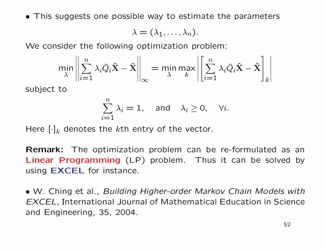
• This suggests one possible way to estimate the parameters

λ = (λ1, . . . , λn).

We consider the following optimization problem:

minλ

∣∣∣∣∣∣∣∣∣∣∣∣

n∑i=1

λiQ̂iX̂− X̂

∣∣∣∣∣∣∣∣∣∣∣∣∞

= minλ

maxk

∣∣∣∣∣∣ n∑i=1

λiQ̂iX̂− X̂

k

∣∣∣∣∣∣subject to

n∑i=1

λi = 1, and λi ≥ 0, ∀i.

Here [·]k denotes the kth entry of the vector.

Remark: The optimization problem can be re-formulated as anLinear Programming (LP) problem. Thus it can be solved byusing EXCEL for instance.

• W. Ching et al., Building Higher-order Markov Chain Models withEXCEL, International Journal of Mathematical Education in Scienceand Engineering, 35, 2004.

52

Remark: Other norms such as ||.||2 and ||.||1 can also be considered.

The former will result in a quadratic programming problem while

||.||1 will still result in a linear programming problem.

• It is known that in approximating data by a linear function ||.||1gives the most robust answer.

• ||.||∞ avoids gross discrepancies with the data as much as pos-

sible.

• If the errors are known to be normally distributed then ||.||2 is

the best choice.

53

• The linear programming formulation:

minλ

w

subject to ww...w

≥ X̂−[Q̂1X̂ | Q̂2X̂ | · · · | Q̂nX̂

] λ1λ2...λn

,

ww...w

≥ −X̂+[Q̂1X̂ | Q̂2X̂ | · · · | Q̂nX̂

] λ1λ2...λn

,

w ≥ 0,n∑

i=1

λi = 1, and λi ≥ 0, ∀i.

• V. Chvatal, Linear Programming, Freeman, New York, 1983.

54

• For a numerical demonstration, we refer to Example 1. A 2nd-order (n = 2) model for the 3-states (m = 3) categorical sequence.

We have the transition frequency matrices

F (1) =

1 3 36 1 11 3 0

and F (2) =

1 4 12 2 33 1 0

. (13)

From (13) we have the i-step transition probability matrices:

Q̂1 =

1/8 3/7 3/43/4 1/7 1/41/8 3/7 0

and Q̂2 =

1/6 4/7 1/41/3 2/7 3/41/2 1/7 0

(14)

and the stationary distribution

X̂ = (2

5,2

5,1

5)T .

Hence we have

Q̂1X̂ = (13

35,57

140,31

140)T , and Q̂2X̂ = (

29

84,167

420,9

35)T .

55

• To estimate λi we consider the optimization problem:

minλ1,λ2

w

subject to

w ≥2

5−

13

35λ1 −

29

84λ2

w ≥ −2

5+

13

35λ1 +

29

84λ2

w ≥2

5−

57

140λ1 −

167

420λ2

w ≥ −2

5+

57

140λ1 +

167

420λ2

w ≥1

5−

31

140λ1 −

9

35λ2

w ≥ −1

5+

31

140λ1 +

9

35λ2

w ≥ 0, λ1 + λ2 = 1, λ1, λ2 ≥ 0.

• The optimal solution is (λ∗1, λ∗2, w

∗) = (1,0,0.0286). Since λ2 is

zero, the “optimal” model is a first-order model.

56

Proposition 3.2 If Qn is irreducible and aperiodic, λ1, λn > 0 and

n∑i=1

λi = 1

then the model has a stationary distribution X satisfying

(I −n∑

i=1

λiQi)X̄ = 0 and 1T X̄ = 1

and

limt→∞

Xt = X.

• We remark that if λn = 0 then it is not an nth model and if λ1 = 0

then the model is clearly reducible.

57

3.7 The Newsboy’s Problem.

• A newsboy sells newspaper (perishable product) every morn-ing. The cost of each newspaper remains at the end of the day isCo (overage cost) and the cost of each unsatisfied demand is Cs

(shortage cost).

• Suppose that the (stationary distribution) probability density func-tion of the demand D is given by

Prob (D = d) = pd ≥ 0, d = 1,2, . . . ,m. (15)

• To determine the best amount r∗ (order size) of newspaper to beordered such that the expected cost is minimized.

Proposition 3.3: The optimal order size r∗ is the one which satisfies

F (r∗ − 1) <Cs

Cs + Co≤ F (r∗). (16)

Here F (x) =x∑

i=1

pi.

58

Example 2: Suppose that the demand (1,2, . . . ,2k) (m = 2k) fol-lows an Markov process with the transition probability matrix Q ofsize 2k × 2k given by

Q =

0 0 · · · 0 11 0 .. . 00 1 0 .. . ...... . . . . . . . . . 00 · · · 0 1 0

(17)

• Assume that Co = Cs. Clearly the next “demand” can be deter-mined by the state of the current demand, and hence the optimalexpected cost is equal to zero when the first-order Markov modelis used.

• When the classical Newsboy model is used, we note that thestationary distribution of Q is given by

1

2k(1,1, . . . ,1)T .

The optimal ordering size is equal to k by Proposition 2.2 and there-fore the optimal expected cost is Cok.

59

Example 3: A large soft-drink company in Hong Kong faces an

in-house problem of production planning and inventory control.

• Products are labeled as either very high sales volume (state 1),

high sales volume (state 2), standard sales volume (state 3),

low sales volume (state 4) or very low sales volume (state 5).

(m = 5).

• For simplicity, we assume the following symmetric cost matrix:

C =

0 100 300 700 1500

100 0 100 300 700300 100 0 100 300700 300 100 0 1001500 700 300 100 0

(18)

where [C]ij is the assigned penalty cost when the production plan

is for sales volume of State i and the actual sales volume is State j.

60

• We employ high-order Markov model for modeling the sales de-

mand data sequence.

• Optimal production policy can then be derived based on Proposi-

tion 2.2.

• The following table shows the optimal costs based on three dif-

ferent models for three different products.

Products A B CHigh-order Markov Model (n = 3) 11200 9300 10800First-order Markov Model (n = 1) 27600 18900 11100Stationary Model 31900 18900 16300

• W. Ching et al., A Higher-order Markov Model for the Newsboy’s

Problem, Journal of Operational Research Society, 54, 2003.

61

4. Multivariate Markov Model for multiple Categorical DataSequences.

• In many situations, there is a need to consider a number of cate-gorical data sequences (having same number of categories/states)together at the same time because they are related to each other.

(i) Gene Expression Sequences. W. Ching et al., On Construc-tion of Stochastic Genetic Networks Based on Gene Expression Se-quences, International Journal of Neural Systems, 2005.

(ii) Credit Risk Measurements. T. Siu, W. Ching et al, On Multi-variate Credibility Approach for Portfolio Credit Risk Measurement,Quantitative Finance, 2005.

(iii) Sales Demand. W. Ching et al., A Multivariate Markov ChainModel for Categorical Data Sequences and Its Applications in De-mand Prediction, IMA Journal of Management Mathematics, 2002.

• Problem: The conventional first-order Markov chain model for scategorical data sequences of m states has ms states.

62

4.1 The Multivariate Markov Chain Model.

• We propose a multivariate Markov chain model which can cap-ture both the intra- and inter-transition probabilities among thesequences and the number of model parameters is O(s2m2).

• Given s sequences with fixed m, the minimum number of param-

eters required is

(s2

)= O(s2).

• We assume that there are s categorical sequences and each hasm possible states in

M = {1,2, . . . ,m}.

• Let X(k)n be the state probability distribution vector of the kth

sequence at time n. If the kth sequence is in State j at time n then

X(k)n = ej = (0, . . . ,0, 1︸︷︷︸

jth entry

,0 . . . ,0)T .

63

• In our proposed multivariate Markov chain model, we assume the

following relationship:

X(j)n+1 =

s∑k=1

λjkP(jk)X(k)

n , for j = 1,2, · · · , s (19)

where

λjk ≥ 0, 1 ≤ j, k ≤ s ands∑

k=1

λjk = 1, for j = 1,2, · · · , s.

(20)

• The state probability distribution of the kth sequence at time

(n+1) depends on the weighted average of P (jk)X(k)n .

• Here P (jk) is a one-step transition probability matrix from the

states in the kth sequence to the states in the jth sequence.

Here recall that X(k)n is the state probability distribution of the kth

sequences at time n.

64

• In matrix form, we have the following block structure matrix equa-

tion (a compact representation):

Xn+1 ≡

X(1)

n+1

X(2)n+1...

X(s)n+1

=

λ11P

(11) λ12P(12) · · · λ1sP

(1s)

λ21P(21) λ22P

(22) · · · λ2sP(2s)

... ... ... ...

λs1P(s1) λs2P

(s2) · · · λssP (ss)

X(1)n

X(2)n...

X(s)n

≡ QXn

or

Xn+1 = QXn.

Remark: We note that X(j)n is a probability distribution vector.

65

4.2 Some Properties of the Model.

Proposition 4.1: If λjk > 0 for 1 ≤ j, k ≤ s, then the matrix Q hasan eigenvalue equal to one and the eigenvalues of Q have modulusless than or equal to one.

Proposition 4.2: Suppose that P (jk) (1 ≤ j, k ≤ s) are irre-ducible and λjk > 0 for 1 ≤ j, k ≤ s. Then there is a vectorX = [X(1), · · · ,X(s)]T such that

X = QX andm∑

i=1

[X(j)]i = 1, 1 ≤ j ≤ s.

Moreover,

limn→∞Xn = X.

Again the proof depends on Perron-Frobenius theorem.

Remark: Propositions 4.1 and 4.2 still hold if [Λij] is irreducibleand aperiodic .

66

4.3 Parameter Estimation.

4.3.1 Estimations of P (jk).

• We can construct the transition frequency matrix from the ob-

served data sequences. More precisely, we count the transition

frequency f(jk)ijik

from the state ik in the sequence {X(k)n } to the

state ij in the sequence {X(j)n }.

• Therefore we construct the transition frequency matrix for the

sequences as follows:

F (jk) =

f(jk)11 · · · · · · f

(jk)m1

f(jk)12 · · · · · · f

(jk)m2... ... ... ...

f(jk)1m · · · · · · f

(jk)mm

.

67

• From F (jk), we get the estimates for P (jk) as follows:

P̂ (jk) =

p̂(jk)11 · · · · · · p̂

(jk)m1

p̂(jk)12 · · · · · · p̂

(jk)m2... ... ... ...

p̂(jk)1m · · · · · · p̂

(jk)mm

where

p̂(jk)ijik

=f(jk)ijik

m∑ij=1

f(jk)ijik

68

4.4 Estimation of λjk

• We have seen that the multivariate Markov chain has a stationary

vector (joint probability distribution vector) X.

• The vector X can be estimated from the sequences by comput-

ing the proportion of the occurrence of each state in each of the

sequences, and let us denote it by

X̂ = (X̂(1), X̂(2), . . . , X̂(s))T .

One would expect thatλ11P̂

(11) λ12P̂(12) · · · λ1sP̂

(1s)

λ21P̂(21) λ22P̂

(22) · · · λ2sP̂(2s)

... ... ... ...

λs1P̂(s1) λs2P̂

(s2) · · · λssP̂ (ss)

X̂ ≈ X̂. (21)

69

• If ||.||∞ is chosen to minimize the discrepancies then we have the

following optimization problem:

minλ

maxi

∣∣∣∣∣∣ m∑k=1

λjkP̂(jk)X̂(k) − X̂(j)

i

∣∣∣∣∣∣

subject tos∑

k=1

λjk = 1, and λjk ≥ 0, ∀k.

(22)

Remark: Again other norms such as ||.||2 and ||.||1 can also be

considered. The former will result in a quadratic programming

problem while ||.||1 will still result in a linear programming prob-

lem.

70

Problem (22) can be formulated as s linear programming prob-

lems. For each j:

minλ

wj

subject to

wjwj...wj

≥ x̂(j) −Bj

λj1λj2...

λjs

wjwj...wj

≥ −x̂(j) +Bj

λj1λj2...

λjs

,

wj ≥ 0,s∑

k=1

λjk = 1, λjk ≥ 0, ∀k,

(23)

where

Bj = [P̂ (j1)X̂(1) | P̂ (j2)X̂(2) | · · · | P̂ (js)X̂(s)].

71

4.5 A Numerical Demonstration

• Consider s = 2 sequences of m = 4 states:

S1 = {4,3,1,3,4,4,3,3,1,2,3,4}

and

S2 = {1,2,3,4,1,4,4,3,3,1,3,1}.

• By counting the transition frequencies

S1 : 4 → 3 → 1 → 3 → 4 → 4 → 3 → 3 → 1 → 2 → 3 → 4

and

S2 : 1 → 2 → 3 → 4 → 1 → 4 → 4 → 3 → 3 → 1 → 3 → 1

we have

F (11) =

0 0 2 01 0 0 01 1 1 20 0 2 1

and F (22) =

0 0 2 11 0 0 01 1 1 11 0 1 1

.

72

• Moreover by counting the inter-transition frequencies

S1 : 4 3 1 3 4 4 3 3 1 2 3 4↘ ↘ ↘ ↘ ↘ ↘ ↘ ↘ ↘ ↘ ↘

S2 : 1 2 3 4 1 4 4 3 3 1 3 1

and

S1 : 4 3 1 3 4 4 3 3 1 2 3 4↗ ↗ ↗ ↗ ↗ ↗ ↗ ↗ ↗ ↗ ↗

S2 : 1 2 3 4 1 4 4 3 3 1 3 1

We have

F (21) =

1 0 2 00 0 0 10 1 3 01 0 0 2

, F (12) =

0 1 1 00 0 1 02 0 1 21 0 1 1

.

73

• After normalization we have the transition probability matrices:

P̂ (11) =

0 0 2

5 012 0 0 012 1 1

523

0 0 25

13

, P̂ (12) =

0 1 1

4 0

0 0 14 0

23 0 1

423

13 0 1

413

,

P̂ (21) =

12 0 2

5 0

0 0 0 13

0 1 35 0

12 0 0 2

3

, P̂ (22) =

0 0 1

213

13 0 0 013 1 1

413

13 0 1

413

.

• Moreover, we also have

X̂1 = (1

6,1

12,5

12,1

3)T and X̂2 = (

1

3,1

12,1

3,1

4)T

Solving the corresponding linear programming problems, the mul-tivariate Markov models of the two categorical data sequences S1and S2 are then given by X(1)

n+1 = 0.00P̂ (11)X(1)n +1.00P̂ (12)X(2)

n

X(2)n+1 = 0.89P̂ (21)X(1)

n +0.11P̂ (22)X(2)n .

74

Proposition 4.3 [Zhu and Ching (2011)] If λii > 0, Pii is irreducible

(for 1 ≤ i ≤ s), the matrix [λij] is also irreducible and at least one

of Pii is aperiodic then the model has a stationary joint probability

distribution

X = (x(1), · · · ,x(s))T

satisfying

X = QX.

Moreover, we have

limt→∞

Xt = X.

• D. Zhu and W. Ching, A Note on the Stationary Property of High-

dimensional Markov Chain Models, International Journal of Pure and

Applied Mathematics, 66, 2011.

75

5. Concluding Remarks.

5.1 Extension to High-order Multivariate Markov Chain Models

• We assume that there are s categorical sequences with order nand each has m possible states in M . In the proposed model, weassume that the jth sequence at time t = r + 1 depends on all thesequences at times t = r, r − 1, . . . , r − n+1.

• Using the same notations, our proposed high-order (nth-order)multivariate Markov chain model takes the following form:

x(j)r+1 =s∑

k=1

n∑h=1

λ(h)jk P

(jk)h x(k)r−h+1, j = 1,2, . . . , s (24)

where

λ(h)jk ≥ 0, 1 ≤ j, k ≤ s, 1 ≤ h ≤ n

ands∑

k=1

n∑h=1

λ(h)jk = 1, j = 1,2, . . . , s.

76

In fact, if we let

X(j)r = ((x(j)r )T , (x(j)r−1)

T , . . . , (x(j)r−n+1)T )T

for j = 1,2, . . . , s be the nm× 1 vectors.

Then the model can be written as the following matrix form:

Xr+1 ≡

X(1)

r+1

X(2)r+1...

X(s)r+1

=

B(11) B(12) . . . B(1s)

B(21) B(22) . . . B(2s)

... ... ... ...

B(s1) B(s2) . . . B(ss)

X(1)r

X(2)r...

X(s)r

≡ JXr

77

where

B(ii) =

λ(1)ii P

(ii)1 λ

(2)ii P

(ii)2 . . . λ

(n−1)ii P

(ii)n−1 λ

(n)ii P

(ii)n

I 0 . . . 0 00 I . . . 0 0... ... ... ... ...0 . . . 0 I 0

mn×mn

and if i ̸= j then

B(ij) =

λ(1)ij P

(ij)1 λ

(2)ij P

(ij)2 . . . λ

(n−1)ij P

(ij)n−1 λ

(n)ij P

(ij)n

0 0 . . . 0 00 0 . . . 0 0... ... ... ... ...0 . . . 0 0 0

mn×mn

.

• W. Ching et al., Higher-order Multivariate Markov Chains and their

Applications, Linear Algebra and Its Applications, 428 (2-3), 2008.

78

• We define an s× s matrix B̃.

We let B̃ii = 1 for all i = 1,2, . . . , s, and if i ̸= j

B̃ij =

1 if λ(k)ij > 0 for all k

0 otherwise.

Here j = 1,2, . . . , s, k = 1,2, . . . , n.

Proposition 4.4 If λ(1)ii , λ(n)ii > 0, P (ii)

1 is irreducible and at least one

of them is aperiodic (i = 1,2, . . . , s), additionally, B̃ is irreducible,

then the model has a stationary probability distribution X satisfying

X = JX.

Moreover,

limt→∞

Xt = X.

79

5.2 Extension to Negative Correlations

• Theoretical results of the multivariate Markov chains were ob-

tained when λij ≥ 0 (non-negative matrix). It is interesting to study

the properties of the models when λij are allowed to be negative.

• An example of a two-chain model: x(1)n+1

x(2)n+1

=

(λ1,1P

(11) λ1,2I

λ2,1I λ2,2P(22)

) x(1)n

x(2)n

︸ ︷︷ ︸

Positive correlated part

+1

m− 1

(λ1,−1P

(11) λ1,−2I

λ2,−1I λ2,−2P(2,2)

) 1− x(1)n

1− x(2)n

.︸ ︷︷ ︸Negative correlated part

Here λi,j ≥ 0 for i = 1,2 and j = ±1,±2 and∑2

j=−2 λi,j = 1.

• W. Ching, et al., An Improved Parsimonious Multivariate Markov

Chain Model for Credit Risk, Journal of Credit Risk, 5, 2009.

80