wkb solution of the wave equation for a plane angular sector · wkb solution of the wave equation...
TRANSCRIPT

PHYSICAL REVIEW E JULY 1998VOLUME 58, NUMBER 1
WKB solution of the wave equation for a plane angular sector
Ahmad T. Abawi* and Roger F. DashenPhysics Department, University of California, San Diego, La Jolla, California 92093
~Received 31 December 1997; revised manuscript received 10 March 1998
The two angular Lame´ differential equations that satisfy boundary conditions on a plane angular sector~PAS! are solved by the Wentzel-Kramers-Brillouin~WKB! method. The WKB phase constants are derived bymatching the WKB solution with the asymptotic solution of the Weber equation. The WKB eigenvalues andeigenfunctions show excellent agreement with the exact eigenvalues and eigenfunctions. It is shown that thoseWKB eigenvalues and eigenfunctions that contribute substantially to the scattering amplitude from a PAS canbe computed in a rather simple way. An approximate formula for the WKB normalization constant, which isconsistent with the WKB assumptions, is derived and compared with the exact normalization constant.@S1063-651X~98!00507-8#
PACS number~s!: 42.25.2p
tct
en
i, n
is
l.ashe
wheiccBfrKtioch
ith
nam
isem
e
I. INTRODUCTION
In a previous paper@1#, formulas for the Wentzel-Kramers-Brillouin ~WKB! eigenvalues satisfying Dirichleor Neumann boundary condition on a plane angular se~PAS! were reported and the WKB eigenvalues,$n,m%, werecompared with the exact eigenvalues for PAS’s of differcorner angles~60°, 90°, and 120°!. A historical review of thesolution of the wave equation for a PAS was also giventhe above paper. It suffices to say that, to our knowledgeapproximate solution of this problem has been reportedthe literature.
In this paper, the two coupled Lame´ equations are solvedby the WKB method. The WKB analysis in this papervalid for large values ofn. Depending on the sign ofm, oneof the two Lame´ equations has turning points. Whenumu issmall the turning points occur where the angles are smalthis region it proves more accurate to obtain the WKB phconstants by matching it with the asymptotic solution of tWeber equation. For large values ofumu, it is shown that thisphase constant reduces to the phase constant obtainedthe solution is matched with the asymptotic solution of tAiry’s equation as is commonly done in quantum mechan
This paper is organized in the following way: In the seond section the WKB solution is formulated and the WKphase constants are derived. In the third section formulasthe WKB eigenvalues for Dirichlet and Neumann boundaconditions are derived and a comparison between the Wand exact eigenfunctions is presented. The fourth seccontains a derivation of approximate WKB solutions whiare valid for small values ofm/n. Finally, an approximateformula for the WKB normalization constant consistent wWKB assumptions is derived in section five.
II. THE GENERAL SOLUTION
The angular part of the wave equation in the sphero-cocoordinate system are expressed by the two angular L´differential equations@2,1#:
*Present address: Propagation Division, SPAWAR Systems Cter, D881, 53560 Hull Street, San Diego, CA 92152-500l.
PRE 581063-651X/98/58~1!/1051~13!/$15.00
or
t
no
in
Ine
hen
s.-
oryBn
ale
A12k2cos2qd
dqFA12k2cos2qd
dqQ~q!G
1@n~n11!k2sin2q1m#Q~q!50 ~1!
and
A12k82cos2wd
dwFA12k82cos2wd
dwF~w!G
1@n~n11!k82sin2w2m#F~w!50, ~2!
where the sphero-conal coordinate system variablesq andware related to the Cartesian coordinate variables,x, y, andzby
x5r cosqA12k82cos2w,
y5r sin q sin w, ~3!
z5r coswA12k2cos2q,
where
k5cosS b
2 D ,
b is the corner angle andk85A12k2. The range of thevariables is
0<q<p, 0<w<2p, r>0.
The geometry of the sphero-conal coordinate systemshown in Fig. 1. The construction of this coordinate systis described, and its orthogonality proved, in@2#. The WKBsolution of Eqs.~1! and ~2! are respectively given by@1#
n-
1051 © 1998 The American Physical Society

-
t
g
dr-s
e
r-s
y
1052 PRE 58AHMAD T. ABAWI AND ROGER F. DASHEN
Q~q!51
A4 ~n1 12 !2k2sin2q1m
3cosH Eq t
qS ~n1 12 !2k2sin2q1m
12k2cos2qD 1/2
dq1dqJ ,
~4!
and
F~w!51
A4 ~n1 12 !2k82sin2w2m
3cosH Ew t
wS ~n1 12 !2k82sin2w2m
12k82cos2wD 1/2
dw1dwJ .
~5!
Notice that theF solution can be obtained from theQ solu-tion by replacingq with w, m with 2m, andk with k8. Thisis also evident in the differential equations, Eqs.~1! and~2!.For m.0, the turning point for theQ equation,q t50, andthe turning point for theF equation isw t5f t(n,2m,k8).For m,0, w t50 andq t5f t(n,m,k), where
f t~n,m,k!5arcsinS 2m
k2~n1 12 !2D 1/2
.
The above solutions are valid forp2q t.q.q t and p2w t.w.w t . For the regionsq t.q.p2q t and w t.w.p2w t the solutions are given by
Q~q!51
A4 umu2~n1 12 !2k2sin2q
3expH 2E0
qS umu2~n1 12 !2k2sin2q
12k2cos2qD 1/2
dqJ ,
m,0. ~6!
FIG. 1. The geometry of the sphero-conal coordinate systemris the distance from the origin to the pointp.
A similar solution for theF equation which is valid form.0can be obtained from the above equation by replacingumu, k,andq with m, k8, andw, respectively. The solutions given byEqs. ~4! and ~6! are separated by the turning points wherethey are both singular. To match these solutions at the turning points, the Lame´ equation is approximated by anotherdifferential equation at the turning point and then theasymptotic solution of this differential equation is matchedwith the WKB solution of the Lame´ equation. By this pro-cess the phase constantsdq anddw are obtained.
Although the WKB solutions obtained in this paper aregeneral, we are particulary interested in those solutions thacorrespond to the small absolute values of the eigenvaluem.The reason for this is that the expression for the scatterinamplitude for a PAS, derived in a separate paper@3#, con-tains either the eigenfunctions or their derivatives evaluateat the surface of the PAS or its edges. Observe that the suface of the PAS in the sphero-conal coordinate system iq5p and its edges arew50 and w5p. Since the WKBeigenfunctions are decaying exponentials to the left of thturning point near zero and to the right of the turning pointnearp, significant contribution to the solution comes fromthose eigenfunctions that have a turning point near the suface or near the edges. They correspond to eigenfunctionwith small absolute values of the eigenvaluem.
To derive a differential equation that approximates theLame equation at the turning points, we use the followingtransformation:
y~q!5A4 12k2cos2~q!Q~q!.
For n@m@1 this transformation converts Eq.~1! tod2
dq2y~q!1p~q!y~q!50, ~7!
with
p~q!5~n1 1
2 !2k2sin2q1m
~12k2cos2q!.
By using the Liouville transformation@4#
y~x!5S dx
dq D 1/2
y~q!,
Eq. ~7! can be transformed to
d2y
dx2 5H 2S dq
dx D 2
p~q!1S dq
dx D 1/2 d2
dx2F S dq
dx D 21/2G J y.
The first term in the curly brackets can be set equal to ansmooth function ofx @4#, and for smallm/n the second termcan be ignored. Near the turning points~q!1! we set
S dq
dx D 2
p~q!5S x2
41aD , ~8!
resulting in
d2y
dx2 1S x2
46aD y50, ~9!
.

luis
eim
s
c-
eer-
PRE 58 1053WKB SOLUTION OF THE WAVE EQUATION FORA . . .
which is the Weber equation. In the above equation the psign is applicable to theQ equation and the minus signapplicable to theF equation. The parametera is determinedfrom Eq.~8! by requiring that the turning points of the Lam´equation and the Weber equation occur at the same tthus ensuring the regularity ofdq/dx at the turning points:
E0
q tS ~n1 12 !2k2sin2q1m
12k2cos2qD 1/2
dq5E0
2A2aS x2
41aD 1/2
dx.
~10!
A similar equation is obtained for theF equation by replac-ing q t by w t , k by k8, m by 2m, anda by 2a. Oncea isdetermined from the above equation,q andw can be relatedto x by
E0
q tS ~n1 12 !2k2sin2q1m
12k2cos2qD 1/2
dq5E0
xS x2
41aD 1/2
dx.
~11!
and
Ew t
wS ~n1 12 !2k82sin2w2m
12k82cos2wD 1/2
dw5E2Aa
x S x2
42aD 1/2
dx.
~12!
a is found to be
a52
pH ~n1 12 !2k822m
k8A~n1 12 !2k21m
3FPS p
2,
m
~n1 12 !2k82
,eD 2K~e!G J , ~13!
where
e51
k8S m
~n1 12 !2k21m D 1/2
, m.0,
andP is the elliptic integral of the third kind. Form,0 a canbe obtained from the above equation by replacingm by umuand interchangingk8 andk. Equation~13! has a power serieexpansion given by
a51
2kk8x1
k22k82
16k3k83~n1 12 !
x2
1328k2k82
128k5k85~n1 12 !2
x31O~x4!,
where
x5m
n1 12
.
If only the first term in the above expansion is retained,
s
e,
a5m
2kk8~n1 12 !
. ~14!
If this value of a is used in Eqs.~11! and ~12!, near theturning points~small q and w! the above equations respetively yield
x5A2k/k8A~n1 12 !q, x5A2k8/kA~n1 1
2 !w. ~15!
Equation ~9! is the desired differential equation. Thasymptotic solution of this equation will be used to detmine dq anddw .
A. The WKB phase constantsdq and dw
The Weber equation
d2y
dx2 1S x2
42aD y50 ~16!
has solutions@5#
W~a,6x!5223/4~AG1 /G3ye7A2G3 /G1yo!, ~17!
where
ye~x,a!511ax2
2!1S a22
1
2D x4
4!
1S a327
2aD x6
6!1•••, ~18!
yo~x,a!5x1ax3
3!1S a22
3
2D x5
5!
1S a3213
2aD x7
7!1•••, ~19!
and
G1~a!5uG~ 14 1 1
2 ia !u,
G3~a!5uG~ 34 1 1
2 ia !u.
For x@uau the Weber equation has asymptotic solutions@5#
W~a,x!5S 2h~a!
x D 1/2
cosH 1
4x22a ln x1
p
41
1
2f2~a!J
and
W~a,2x!5S 2
h~a!xD 1/2
sinH 1
4x22a ln x1
p
41
1
2f2~a!J ,
where
h~a!5A11e2pa2epa, f2~a!5argG@ 12 1 ia#.
From these two solutions we construct an even solution

e
D
ir
ith
om-
ob-ary
1054 PRE 58AHMAD T. ABAWI AND ROGER F. DASHEN
ye~x,a!5A4 2S G3~a!
G1~a! D1/2S 11h2~a!
h~a! D 1/2S 1
xD 1/2
3cosH x2
42a ln x1
p
41
1
2f2~a!2g~a!J ,
~20!
and an odd solution
yo~x,a!52A4 2S G1~a!
2G3~a! D1/2S 11h2~a!
h~a! D 1/2S 1
xD 1/2
3cosH x2
42a ln x1
p
41
1
2f2~a!1g~a!J ,
~21!
where
tang~a!51
h~a!5A11e2pa1epa.
In the region wherew is small so that the Lame´ equation canbe approximated by the Weber equation, yetn is large so thatthe WKB solution for the Lame´ equation is valid, and
x5S 2k8
k D 1/2S n11
2D 1/2
w@uau,
both Eq.~5! and Eqs.~20! or ~21! are solutions of the samdifferential equation. The phase constantdw can therefore bedetermined by matching the phases of the two solutions.pending on the prescribed boundary conditions, eitherye oryo will be employed to obtain these phase constants. Fconsider the even solution for theF equation. From Eq.~12!we have
I w5Ew t
wS ~n1 12 !2k82sin2w2m
12k82cos2wD 1/2
dw
51
2E2Aa
xAx224a dx
5x
4Ax224a2a ln@x1Ax224a#1a ln@2Aa#.
Expanding the last expression in powers ofa and keepingonly terms of first order gives
I w5x2
42a ln x1
a
2lnuau2
a
2.
The WKB solution, Eq.~5!, thus becomes
F~x!5AwA4 2
A4 ~n1 12 ! kk8Ax
3cosH x2
42a lnx1
a
2lnuau2
a
21dwJ .
e-
st
Comparing the phase and amplitude of this equation wthat of ye(x,a) we find
dw5p
41
1
2f2~a!2g~a!2
a
2lnuau1
a
2
and
Aw5A4 kk8~n1 12 !S G3~a!
G1~a! D1/2S 11h2~a!
h~a! D 1/2
. ~22!
It can be shown that
2g~a!23
4p5arctanF tanhS pa
2 D G[D~a!52D~2a!.
In terms of this new quantity we have
dw52p
81
1
2f2~a!2
1
2D~a!2
a
2lnuau1
a
2. ~23!
The phase constant for the odd solution is obtained by cparing I w with the phase of Eq.~21!. It is
dw855p
81
1
2f2~a!1
1
2D~a!2
a
2lnuau1
a
2.
A similar analysis gives
dq52p
81
1
2f2~2a!1
1
2D~a!1
a
2lnuau2
a
2~24!
and
Aq5A4 ~n1 12 !kk8S G3~2a!
G1~2a! D1/2S 11h2~2a!
h~2a! D 1/2
.
~25!
And for the odd solution we find
dq8 55p
81
1
2f2~2a!2
1
2D~a!1
a
2lnuau2
a
2.
For m , 0 the role of theF and theQ equations are inter-changed. In other words, in this case theQ equation is theone with the turning points. However, the expressionstained for the phase constants still remain valid. In summwe have
dw52p
81
1
2f2~a!2
1
2D~a!2
a
2lnuau1
a
2,
dq52p
82
1
2f2~a!1
1
2D~a!1
a
2lnuau2
a
2,
dw855p
81
1
2f2~a!1
1
2D~a!2
a
2lnuau1
a
2,
dq8 55p
82
1
2f2~a!2
1
2D~a!1
a
2lnuau2
a
2.
s
au
ohe
lu
ing
-nn
PRE 58 1055WKB SOLUTION OF THE WAVE EQUATION FORA . . .
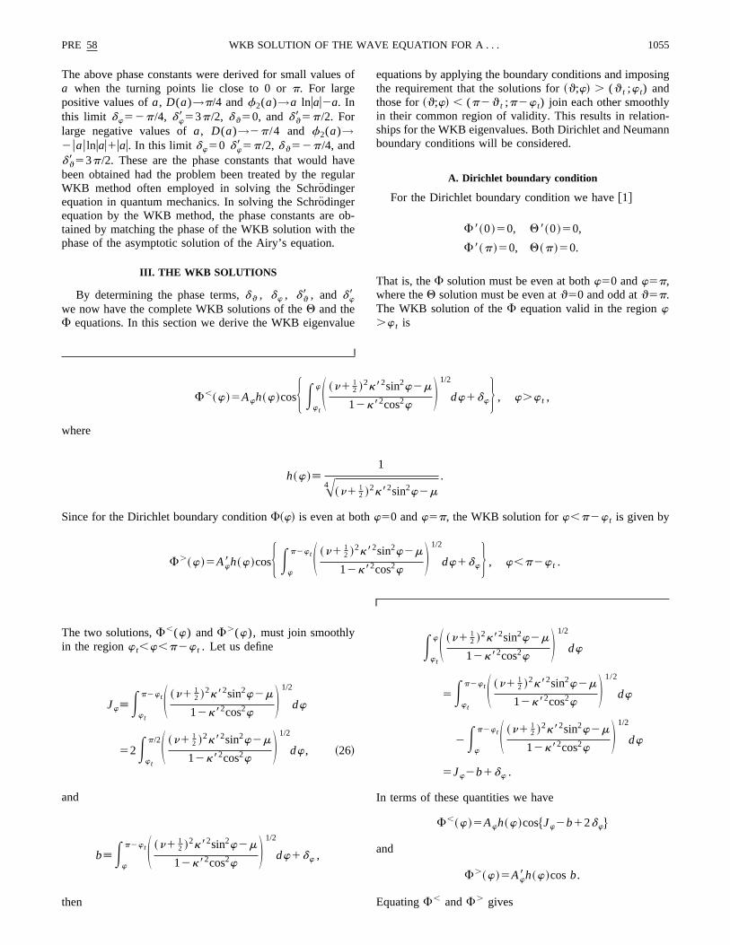
The above phase constants were derived for small valuea when the turning points lie close to 0 orp. For largepositive values ofa, D(a)→p/4 andf2(a)→a lnuau2a. Inthis limit dw52p/4, dw853p/2, dq50, anddq8 5p/2. Forlarge negative values ofa, D(a)→2p/4 and f2(a)→2uau lnuau1uau. In this limit dw50 dw85p/2, dq52p/4, anddq8 53p/2. These are the phase constants that would hbeen obtained had the problem been treated by the regWKB method often employed in solving the Schro¨dingerequation in quantum mechanics. In solving the Schro¨dingerequation by the WKB method, the phase constants aretained by matching the phase of the WKB solution with tphase of the asymptotic solution of the Airy’s equation.
III. THE WKB SOLUTIONS
By determining the phase terms,dq , dw , dq8 , and dw8we now have the complete WKB solutions of theQ and theF equations. In this section we derive the WKB eigenva
of
velar
b-
e
equations by applying the boundary conditions and imposthe requirement that the solutions for~q;w! . (q t ;w t) andthose for~q;w! , (p2q t ;p2w t) join each other smoothlyin their common region of validity. This results in relationships for the WKB eigenvalues. Both Dirichlet and Neumaboundary conditions will be considered.
A. Dirichlet boundary condition
For the Dirichlet boundary condition we have@1#
F8~0!50, Q8~0!50,
F8~p!50, Q~p!50.
That is, theF solution must be even at bothw50 andw5p,where theQ solution must be even atq50 and odd atq5p.The WKB solution of theF equation valid in the regionw.w t is
F,~w!5Awh~w!cosH Ew t
wS ~n1 12 !2k82sin2w2m
12k82cos2wD 1/2
dw1dwJ , w.w t ,
where
h~w
1056 PRE 58AHMAD T. ABAWI AND ROGER F. DASHEN
Aw$cos$Jw12dw%cosb1sin$Jw12dw%sin b%5Aw8cosb.
The solution to this equation, which givesAw8 , constant andindependent of the parameterb, is obtained by setting
Jw12dw5mp, m50,1, . . . .
t o
s
Substituting fordw , we find
Jw1f2~a!2D~a!2a lnuau1a5~m1 14 !p, m50,1, . . . .
For Dirichlet boundary conditionQ~q! is even aroundq50and odd aroundq5p. Then
Q,~q!5Aqh~q!cosH Eq t
qS ~n1 12 !2k2sin2q1m
12k2cos2qD 1/2
dq1dqJ , q.0,
whereh~q! is h~w! with the appropriate change of variables. The solution forq.p1q t is
Q.~q!5Aq8 h~q!cosH Ep1q t
q S ~n1 12 !2k2sin2q1m
12k2cos2qD 1/2
dq1dq8 J , q.p1q t .
Since this solution is odd with respect toq5p, the solution forq,p2q t is given by
Q.~q!52Aq8 h~q!cosH Eq
p2q tS ~n1 12 !2k2sin2q1m
12k2cos2qD 1/2
dq1dq8 J , q,p2q t .
ty
Requiring thatQ,(q) andQ.(q) join each other smoothlyresults in
Jq1dq1dq8 5np, n51,2, . . . .
Note that the reasonn starts from 1 is to guarantee that
np2dq2dq8 .0,
sinceJq is positive. Substituting fordq anddq8 we find
Jq1f2~2a!1a lnuau2a5~n1 12 !p, n50,1, . . . .
For Dirichlet boundary condition we therefore have the seeigenvalue equations
Jw1f2~a!2D~a!2a lnuau1a5~m1 14 !p, m50,1, . . . ,
Jq1f2~2a!1a lnuau2a5~n1 12 !p, n50,1, . . . .
~27!
The integrals defined byJq andJw can be expressed in termof elliptic integrals@6#
Jq52m
k8A~n1 12!
2k21mH PS p
2,
~n1 12!
2k2
~n1 12!
2k21m,r 1D J ,
and
Jw52m
k8A~n1 12!
2k21m
3H PS p
2,~n1 1
2!2k822m
~n1 12!
2k82,r 1D 2K~r 1!J
f
for m.0 and
Jq522m
kA~n1 12!
2k822m
3H PS p
2,~n1 1
2!2k21m
~n1 12!
2k2,r 2D 2K~r 2!J ,
and
Jw522m
kA~n1 12!
2k822mH PS p
2,
~n1 12!
2k82
~n1 12!
2k822m,r 2D J
for m , 0. In the above
r 15k
k8S ~n1 1
2!2k822m
~n1 12!
2k21mD 1/2
,
r 25k8
k S ~n1 12!
2k22m
~n1 12!
2k821mD 1/2
,
P is the elliptic integral of the third kind, andK is the ellipticintegral of the first kind. We also have the following identifor Jq andJw :
Jq1Jw5~n1 12 !p. ~28!

xact
PRE 58 1057WKB SOLUTION OF THE WAVE EQUATION FORA . . .
FIG. 2. The top two panels show theQ and theF eigenfunctions for the exact~solid lines!, the WKB ~dashed lines! and the power seriessolution to the Weber equation~dotted lines! of the Lameequations, subject to Dirichlet boundary condition. The corresponding eeigenvalues are~n,m!5~6.282 285,0.442 731!, and the corresponding WKB eigenvalues are~n,m!5~6.282 324,0.441 515!. The bottom twopanels show the same eigenfunctions for Neumann boundary condition with exact eigenvalues~n,m!5~6.792 665,20.632 047! and WKBeigenvalues~n,m!5~6.792 723,20.630 761!. Note how the power series solutions overlay the exact solutions forq andw close to zero andp and connect smoothly with the WKB solutions.
-
e
tth
val-
nc-
l a
m-hen-
ualthehen
er.
B. Neumann boundary condition
For the Neumann boundary condition we have
F~0!50, Q~0!50,
F~p!50, Q8~p!50.
The F solution is thus odd with respect tow50 andw5pwhere theQ solution is odd with respect toq50 and evenwith respect toq5p. A similar approach yields the eigenvalue equations:
Jw1f2~a!1D~a!2a lnuau1a5~m1 34 !p, m50,1, . . .
Jq1f2~2a!1a lnuau2a5~n1 12 !p, n50,1, . . . .
~29!
Note that Eqs.~27! and ~29! are two parameter eigenvaluequations. This means that for a given value ofn andm eachset of equations must be solved simultaneously. We usedNewton-Raphson method in two dimensions to compute
hee
eigenvalues,n andm for each boundary condition. The WKBeigenvalues agree remarkably well with the exact eigenues@1#.
C. The WKB eigenfunctions
Once the eigenvalues are computed, the WKB eigenfutions can be obtained from Eqs.~4! and~5!. It is obvious thateither of these solutions multiplied by a constant is stilsolution. However, the amplitudesAq and Aw were deter-mined in such a way that the WKB solutions can be copared with the exact solution and with the solution of tWeber equation without the need to multiply them by a costant. This proves convenient when comparing individeigenfunctions. The complete normal mode solution ofwave equation for this problem involves a sum over tproduct of all eigenfunctions divided by the normalizatioconstant that removes any amplitude ambiguities@3#. TheWKB normalization constant is derived later in this papFor even solutions the amplitudesAq andAw given by Eqs.

therf
fo
te0
de
ns
yay
Ica
heth
l-Kn
d-
let
1058 PRE 58AHMAD T. ABAWI AND ROGER F. DASHEN
~25! and ~22! are determined such thatz(0)51 andz8(0)50, wherez can be eitherQ or F. For odd solutions, on theother hand, the initial conditions arez(0)50 and z8(0)51. Because the derivative of the solution is nonzero atinitial point, Aq and Aw must be multiplied by the scalfactorsdq/dx anddw/dx, respectively. To see this, take, foexample,Q~q!, which nearq50 reduces to the solution othe Weber equation,y(x). Then
dQ~q!
dq Uq50
;dy~x!
dq Uq50
5dy~x!
dx Ux50
dx
dq51.
Sincedy/dxux50 is chosen to be unity,Q~q! multiplied bydq/dx satisfies the above equation. The same is trueF~w!. dq/dx anddw/dx may be obtained from Eq.~15!.
As was pointed out before, we are particularly interesin those solutions for which the turning points lie close toor p. In this case near 0 andp the solution can be obtainefrom the power series solution of the Weber equation givby Eqs.~18! and~19!. For a given set of eigenvalues$n,m%, ais determined from Eq.~10!. Then the power series solutioare obtained by choosingq or w as independent variableand determiningx from Eqs.~11! or ~12!, which is then usedin Eqs. ~18! and ~19!. The results are shown in Fig. 2. Bonly using a few terms, the power series solution overlthe exact solution forq and w close to zero andp andsmoothly connects with the WKB solution in each case.this way an excellent approximation to the exact solutionbe obtained for the entire interval between 0 andp.
IV. SOLUTION FOR LARGE n AND SMALL m
It was pointed out earlier that the main contribution to tscattering amplitude comes from those eigenfunctionscorrespond to small values ofm. It will be shown in thissection that whenm/n2!1, the expressions for the eigenvaues and the integrals appearing in the phases of the Wsolutions can be approximated by simple algebraic functioFirst, consider the integral
tio
ly
e
r
d
n
s
nn
at
Bs.
Jq5E0
pS ~n1 12!
2k2sin2q1m
12k2cosqD 1/2
52k
k8 S n11
2D E0
p/2 Asin2q1a
A11z sin2qdq,
where
a5m
k2~n1 12!
25
2ak8
k~n1 12!
, z5S k
k8D 2
.
For small values ofa this integral is approximated by@7#
Jq52~n1 12 !arctan
k
k81a ln@8kk8~n1 1
2 !#
2a lnuau1a1O~a2!. ~30!
Similarly,
Jw52~n1 12 !arctan
k8
k2a ln@8kk8~n1 1
2 !#
1a lnuau2a1O~a2!. ~31!
By adding the eigenvalue equations for the Dirichlet bounary condition, Eq.~27!, and using Eq.~28! we find
n5m1n11
41
D~a!
p. ~32!
For Neumann boundary condition we similarly find
n5m1n13
42
D~a!
p. ~33!
By subtracting the eigenvalue equations for the Dirichboundary condition and using Eqs.~30!, ~31!, and ~32! wefind
2S m1n13
41
D~a!
p D S p
22b D12a lnF8kk8S m1n1
3
41
D~a!
p D G22f2~a!1D~a!5S n2m11
4Dp. ~34!
In the same way we find for the Neumann boundary condition
2S m1n15
42
D~a!
p D S p
22b D12a lnF8kk8S m1n1
5
42
D~a!
p D G22f2~a!2D~a!5S n2m21
4Dp. ~35!
e
on
ee-KB
In the above equations use has been made of the relaships
arctank8
k5
b
2, arctan
k
k85S p
22
b
2 D .
Equations~34! and ~35! have the advantage that they on
n-depend on the parametera. This allows one to solve thesequations fora by performing a search in one dimension~asopposed to two dimensions when the equations dependnas well! and then use Eqs.~32! and~33! to determinen. Theeigenvalues obtained in this way are still in excellent agrment with the exact eigenvalues. The phase of the Wsolution for theQ equation, Eq.~4! is

ion
d
hes
ror-
r
PRE 58 1059WKB SOLUTION OF THE WAVE EQUATION FORA . . .
f ~q!5Eq t
qS ~n1 12!
2k2sin2q1m
12k2cos2qD 1/2
dq1dq .
This can be written asf~q!5f~p/2!2u~q!, ~36!
where
f S p
2 D5Eq t
p/2S ~n1 12!
2k2sin2q1m
12k2cos2qD 1/2
dq1dq ,
and
u~q!5Eq
p/2S ~n1 12!
2k2sin2q1m
12k2cos2qD dq
5kS n11
2D Eq
p/2 Asin2q1v
A12k2cos2qdq,
where
v5m
k2~n1 12!
2.
Using the WKB eigenvalue equations and the expressfor dq and dw , we find for both Dirichlet and Neumanboundary conditions
f S p
2 D51
2S n11
4Dp1D~a!
2.
Similarly the phase of theF equation can be written as
g~w!5gS p
2 D2u~w!.
For the Dirichlet boundary condition we find
gS p
2 D 5mp
2,
and for the Neumann boundary condition we find
gS p
2 D51
2S m11
2Dp2D~a!.
In the aboveg~w! is f ~q! with k replaced byk8, m by 2m,anddq by dw . For smallv it may be shown that@7#
u~q!5S n11
2Darcsin@k cosq#
1a lnU A12k2cos2q1k8cosq
sinqU, ~37!
wherea5m/2kk8(n1 12). A similar solution can be obtaine
for u~w! by replacingk with k8 anda with 2a.
ns
V. THE WKB NORMALIZATION
In this section we derive an approximate formula for tWKB normalization coefficient that is valid for small valueof m and large values ofn. The normalization coefficent fothe solution of the wave equation in the sphero-conal codinate system is given by@2#
N5E0
pE0
p
uQLame~q!FLame~w!u2sdq dw, ~38!
where
s5k2sin2q1k82sin2w
A~12k2cos2q!~12k82cos2w!.
Let us define
xLame~q
efo
tio
be
re
ov
l
reye
1060 PRE 58AHMAD T. ABAWI AND ROGER F. DASHEN
E0
p
@xLame~q!2xLameWKB~q!#y~q!dq
5E0
D
@xLame~q!2xLameWKB~q!#y~q!dq
1ED
p2D
@xLame~q!2xLameWKB~q!#y~q!dq
1Ep2D
p
@xLame~q!2xLameWKB~q!#y~q!dq.
Since forq close to 0 orp the Lameequation reduces to thWeber equation,D is chosen to be small enough such that0,q,D andp2D,q,p, the solution of the Lame´ equationcan be represented by the solution of the Weber equadenoted byxWeber, and the WKB solution of the Lame´ equa-tion can be represented by the WKB solution of the Weequation, denoted byxWeber
WKB , and given by Eqs.~20! or ~21!.In the regionD,q,p2D, both the solution of the Lame´equation and the solution of the Weber equation can beresented by their WKB solutions:
xLame~q!5xLameWKB~q!, xWeber~q!5xWeber
WKB ~q!.
Based on this argument the middle integral in the abequation is zero and in the other integralsxLame can be re-placed byxWeber, resulting in
E0
p
@xLame~q!2xLameWKB~q!#y~q!dq
5E0
D
@xWeber~q!2xWeberWKB ~q!#y~q!dq
1Ep2D
p
@xWeber~q!2xWeberWKB ~q!#y~q!dq.
Substituting these in Eq.~40! we find
E0
p
xLame~q!y~q!dq
5E0
D
@xWeber~q!2xWeberWKB ~q!#y~q!dq
1Ep2D
p
@xWeber~q!2xWeberWKB ~q!#y~q!dq
1E0
p
xLameWKB~q!y~q!dq.
In the second integral in the above equation letq85p2q, so
Ep2D
p
@xWeber~q!2xWeberWKB ~q!#y~q!dq
5E0
D
@xWeber~q8!2xWeberWKB ~q8!#y~q8!dq8.
Next, let us write
r
n,
r
p-
e
E0
D
@xWeber~q!2xWeberWKB ~q!#y~q!dq
5E0
`
@xWeber~q!2xWeberWKB ~q!#y~q!dq
2ED
`
@xWeber~q!2xWeberWKB ~q!#y~q!dq.
For q.D, xWeber~q!5xWeberWKB ~q! and thus the second integra
in the above equation is zero and
E0
D
@xWeber~q!2xWeberWKB ~q!#y~q!dq
5E0
`
@xWeber~q!2xWeberWKB ~q!#y~q!dq.
Thus
E0
p
xLame~q!y~q!dq
5E0
`
@xWeber~q!2xWeberWKB ~q!#y~q!dq
1E0
`
@xWeber~q8!2xWeberWKB ~q8!#y~q!8dq8
1E0
p
xLameWKB~q!y~q!dq. ~41!
Note that in the first integral the functions in the squabrackets are valid nearq50 and in the second integral theare valid nearq5p. In the equation for the normalization weither have
y~q!5k2sin2q
A12k2cos2q
or
y~q!51
A12k2cos2q.
In the first case we have
E0
p
xLame~q!k2sin2q
A12k2cos2dq
5E0
`
@xWeber~q!2xWeberWKB ~q!#
k2sin2q
A12k2cos2qdq
1E0
`
@xWeber~q8!2xWeberWKB ~q8!#
k2sin2~q8!
A12k2cos2q8dq8
1E0
p
xLameWKB~q!
k2sin2q
A12k2cos2qdq.

ls
o
e
a-
0
PRE 58 1061WKB SOLUTION OF THE WAVE EQUATION FORA . . .
There is negligible contribution from the first two integraon the right hand side because for small values ofq, sinq'0 and for large values ofq, xWeber(q) 5 xWeber
WKB (q).Therefore, we find
E0
p
xLame~q!k2sin2q
A12k2cos2qdq
5E0
p
xLameWKB~q!
k2sin2q
A12k2cos2qdq.
In the second case
E0
p
xLame~q!1
A12k2cos2qdq
5E0
`
@xWeber~q!2xWeberWKB ~q!#
1
A12k2cos2qdq
1E0
`
@xWeber~q8!2xWeberWKB ~q8!#
1
A12k2cos2q8dq8
1E0
p
xLameWKB~q!
1
A12k2cos2qdq.
Here again there is negligible contribution from the first twintegrals for large values ofq sincexWeber(q)5xWeber
WKB (q).For small valuers ofq
1
A12k2cos2q'
1
k8,
and thus we have
E0
p
xLame~q!1
A12k2cos2qdq
51
k8E
0
`
@xWeber~q!2xWeberWKB ~q!#dq
11
k8E
0
`
@xWeber~q8!2xWeberWKB ~q8!#dq8
1E0
p
xLameWKB~q!
1
A12k2cos2qdq.
Let us define
eq5E0
`
@xWeber~q!2xWeberWKB ~q!#dq,
and
eq8 5E0
`
@xWeber~q8!2xWeberWKB ~q8!#dq8,
then
E0
p
xLame~q!1
A12k2cos2qdq
5eq1eq8
k81E
0
p
xLameWKB~q!
1
A12k2cos2qdq.
Following a similar procedure using integrals involving thvariablew and substituting in Eq.~38! yields
N5E0
p k2sin2~q!xLameWKB~q!
A12k2cos2qdq
3FCw
ew1ew8
k1E
0
p xLameWKB~w!
A12k82cos2wdwG
1E0
p k82sin2~w!xLameWKB~w!
A12k82cos2wdw
3FCq
eq1eq8
k81E
0
p xLameWKB~q!
A12k2cos2qdqG , ~42!
where
ew5E0
`
@xWeber~w!2xWeberWKB ~w!#dw,
and
ew85E0
`
@xWeber~w8!2xWeberWKB ~w8!#dw8,
andCq andCw are proportionality constants given by
E cLame~q!2dq5CqE cWeber2 ~x!dx, ~43!
and
TABLE I. Comparison between the exact and WKB normaliztion coefficients.
(n,m) aexact aWKB Nexact NWKB
~1,1! 0.465 255 0.324 84 3.8244 3.3266~2,1! 20.452 788 20.348 023 2.9522 3.0724~2,2! 0.530 210 0.504 450 5.0025 4.8042~3,1! 20.549 215 20.537 476 8.4871 8.7563~3,2! 0.057 476 0.055 747 1.3784 1.3586~3,3! 0.617 823 0.611 585 19.0350 18.5510~4,1! 20.652 852 20.651 458 41.9459 41.1747~4,2! 20.126 564 20.124 423 1.4276 1.4592~4,3! 0.204 048 0.201 308 2.2521 2.2066~4,4! 0.691 944 0.694 140 98.7856 93.2777~5,1! 20.720 185 20.725 213 229.3953 211.8818~5,2! 20.251 494 20.244 911 3.7883 3.8674~5,3! 0.029 370 0.029 055 0.8805 0.8758~5.4! 0.309 851 0.308 281 7.8471 7.7465~5,5! 0.745 515 0.752 932 539.3419 480.618
ef
lts
thfoarffin
o
ica-er
1062 PRE 58AHMAD T. ABAWI AND ROGER F. DASHEN
E cLame~w!2dw5CwE cWeber2 ~x!dx. ~44!
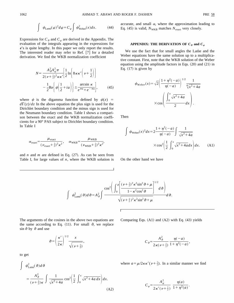
Expressions forCq andCw are derived in the Appendix. Thevaluation of the integrals appearing in the expressionse’s is quite lengthy. In this paper we only report the resuThe interested reader may refer to Ref.@7# for a detailedderivation. We find the WKB normalization coefficient
N5Aq
2 Aw2p
2~n1 12!
2kk8F1
2lnH 8kk8S n1
1
2D J2
1
2ReH cS 1
21 ia D J 6
arcsink
epa1e2paG , ~45!
where c is the digamma function defined byc(z) 5dG(z)/dz In the above equation the plus sign is used forDirichlet boundary condition and the minus sign is usedthe Neumann boundary condition. Table I shows a compson between the exact and the WKB normalization coecients for a 90° PAS subject to Dirichlet boundary conditioIn Table I
aexact5mexact
~nexact112!
2k2, aWKB5
mWKB
~nWKB1 12!
2k2,
and n and m are defined in Eq.~27!. As can be seen fromTable I, for large values ofn, where the WKB solution is
a
or.
eri--.
accurate, and smalla, where the approximation leading tEq. ~45! is valid, NWKB matchesNexact very closely.
APPENDIX: THE DERIVATION OF Cq and Cw
We use the fact that for small angles the Lam´ e and theWeber equations have the same solution up to a multipltive constant. First, note that the WKB solution of the Webequation using the amplitude factors in Eqs.~20! and~21! inEq. ~17! is given by
cWeber~x!5A2S 11h2~2a!
h~2a! D 1/2 1
A4 x214a
3cosS E0
xAx214a
2dxD .
Then
E cWeber~x!2dx5211h2~2a!
h~2a!E 1
Ax214a
3cos2S 1
2 E0
xAx214adxD dx. ~A1!
On the other hand we have
E cLame2 ~q!dq5Aq
2 Ecos2S E
0
qF ~n1 12!
2k2sin2q1m
12k2cos2qG 1/2
dq DA~n1 1
2 !2k2sin2q1mdq.
The arguments of the cosines in the above two equationsthe same according to Eq.~11!. For small q, we replacesinq by q and use
q5S k8
2kD 1/2 x
A~n1 12!
,
to get
E cLame2 ~q!dq
5Aq
2
~n1 12!k
E 1
Ax214acos2S 1
2 E0
xAx214a dxD dx.
~A2!
reComparing Eqs.~A1! and ~A2! with Eq. ~43! yields
Cq5Aq
2
2k~n1 12!
h~2a!
11h2~2a!,
wherea5m/2kk8(n1 12). In a similar manner we find
Cw5Aw
2
2k8~n1 12 !
h~a!
11h2~a!.
J
,
n
PRE 58 1063WKB SOLUTION OF THE WAVE EQUATION FORA . . .
@1# Ahmad T. Abawi, Roger F. Dashen, and Herbert Levine,Math. Phys.38, 1623~1997!.
@2# L. Kraus and L. Levine, Commun. Pure Appl. Math.9, 49~1961!.
@3# Ahmad T. Abawi and Roger F. Dashen, Phys. Rev. E56, 2172~1997!.
@4# F. W. J. Olver,Asymptotics and Special Functions~Academic,
. New York, 1974!.@5# Handbook of Mathematical Functions, edited by M.
Abramowitz and I. A. Stegun~Dover, New York, 1972!.@6# I. S. Gradshteyn and I. M. Ryzhik,Tables of Integrals, Series
and Products, 2nd ed.~Academic, New York, 1980!.@7# Ahmad T. Abawi, Ph.D. thesis, University of California, Sa
Diego, 1993.