w.j. riley hamilton technical services beaufort, sc 29907 frequency standard primer 102211.pdf ·...
TRANSCRIPT

W.J. Riley
Hamilton Technical Services
Beaufort, SC 29907
RUBIDIUM FREQUENCY STANDARD PRIMER
ii
Copyright Notice
© 2010-2011 Hamilton Technical Services
All Rights Reserved
No part of this document may be reproduced or retransmitted in any form or by any
means, electronically or mechanically, including photocopying or scanning, for any
purpose other than the purchaser‟s personal use, without the express written
permission of Hamilton Technical Services. The information in this document is
provided without any warranty of any type. Please report any errors or beneficial
comments to the address below.
Rubidium Frequency Standard Primer
10/22/2011
Available from www.lulu.com as ID # 9559425
Hamilton Technical Services Phone: 843-525-6495
650 Distant Island Drive Fax: 843-525-0251
Beaufort, SC 29907-1580 E-Mail: [email protected]
USA Web: [email protected]
Cover photograph: Classic Efratom FRK and modern Symmetricom X72 rubidium
frequency standards.

FRONT MATTER
iii
About the Author
William J. Riley, Jr.
Proprietor
Hamilton Technical Services
650 Distant Island Drive
Beaufort, SC 29907
Phone: 843-525-6495
Fax: 843-525-0251
E-Mail: [email protected]
Web: www.wriley.com
Mr. Riley has worked in the area of frequency control his entire professional career.
He is currently the Proprietor of Hamilton Technical Services, where he provides
software and consulting services in that field, including the Stable program for the
analysis of frequency stability. Bill collaborates with other experts in the time and
frequency community to provide an up-to-date and practical tool for frequency
stability analysis that has received wide acceptance within that community. From
1999 to 2004, he was Manager of Rubidium Technology at Symmetricom, Inc.
(previously Datum), applying his extensive experience with atomic frequency
standards to those products within that organization, including the early development
of a chip-scale atomic clock (CSAC). From 1980-1998, Mr. Riley was the
Engineering Manager of the Rubidium Department at EG&G (later PerkinElmer and
now Excelitas), where his major responsibility was to direct the design of rubidium
frequency standards, including high-performance rubidium clocks for the GPS
navigational satellite program. Other activities there included the development of
several tactical military and commercial rubidium frequency standards. As a
Principal Engineer at Harris Corporation, RF Communications Division in 1978-
1979, he designed communications frequency synthesizers. From 1962-1978, as a
Senior Development Engineer at GenRad, Inc. (previously General Radio), Mr.
Riley was responsible for the design of electronic instruments, primarily in the area
of frequency control. He has a 1962 BSEE degree from Cornell University and a
1966 MSEE degree from Northeastern University. Mr. Riley holds six patents in the
area of frequency control, and has published a number of papers and tutorials in that
field. He is a Fellow of the IEEE, and a member of Eta Kappa Nu, the IEEE UFFC
Society, and served on the Precise Time and Time Interval (PTTI) Advisory Board.
He received the 2000 IEEE International Frequency Control Symposium I.I. Rabi
Award for his work on atomic frequency standards and frequency stability analysis,
and the 2011 Distinguished PTTI Service Award recognizing outstanding
contributions related to PTTI systems.
RUBIDIUM FREQUENCY STANDARD PRIMER
iv
Dedication
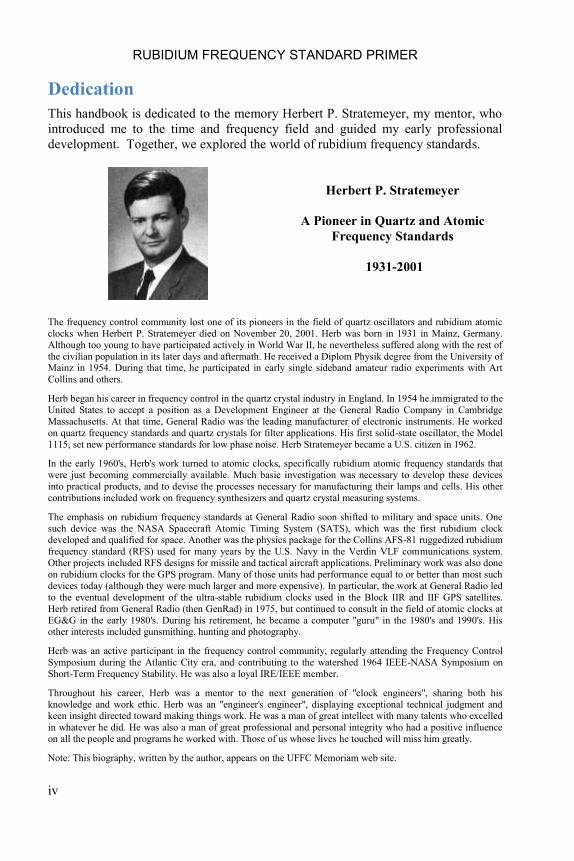
This handbook is dedicated to the memory Herbert P. Stratemeyer, my mentor, who
introduced me to the time and frequency field and guided my early professional
development. Together, we explored the world of rubidium frequency standards.
Herbert P. Stratemeyer
A Pioneer in Quartz and Atomic
Frequency Standards
1931-2001
The frequency control community lost one of its pioneers in the field of quartz oscillators and rubidium atomic
clocks when Herbert P. Stratemeyer died on November 20, 2001. Herb was born in 1931 in Mainz, Germany.
Although too young to have participated actively in World War II, he nevertheless suffered along with the rest of
the civilian population in its later days and aftermath. He received a Diplom Physik degree from the University of Mainz in 1954. During that time, he participated in early single sideband amateur radio experiments with Art
Collins and others.
Herb began his career in frequency control in the quartz crystal industry in England. In 1954 he immigrated to the
United States to accept a position as a Development Engineer at the General Radio Company in Cambridge
Massachusetts. At that time, General Radio was the leading manufacturer of electronic instruments. He worked
on quartz frequency standards and quartz crystals for filter applications. His first solid-state oscillator, the Model
1115, set new performance standards for low phase noise. Herb Stratemeyer became a U.S. citizen in 1962.
In the early 1960's, Herb's work turned to atomic clocks, specifically rubidium atomic frequency standards that
were just becoming commercially available. Much basic investigation was necessary to develop these devices
into practical products, and to devise the processes necessary for manufacturing their lamps and cells. His other
contributions included work on frequency synthesizers and quartz crystal measuring systems.
The emphasis on rubidium frequency standards at General Radio soon shifted to military and space units. One
such device was the NASA Spacecraft Atomic Timing System (SATS), which was the first rubidium clock developed and qualified for space. Another was the physics package for the Collins AFS-81 ruggedized rubidium
frequency standard (RFS) used for many years by the U.S. Navy in the Verdin VLF communications system.
Other projects included RFS designs for missile and tactical aircraft applications. Preliminary work was also done
on rubidium clocks for the GPS program. Many of those units had performance equal to or better than most such
devices today (although they were much larger and more expensive). In particular, the work at General Radio led
to the eventual development of the ultra-stable rubidium clocks used in the Block IIR and IIF GPS satellites.
Herb retired from General Radio (then GenRad) in 1975, but continued to consult in the field of atomic clocks at
EG&G in the early 1980's. During his retirement, he became a computer "guru" in the 1980's and 1990's. His other interests included gunsmithing, hunting and photography.
Herb was an active participant in the frequency control community, regularly attending the Frequency Control
Symposium during the Atlantic City era, and contributing to the watershed 1964 IEEE-NASA Symposium on
Short-Term Frequency Stability. He was also a loyal IRE/IEEE member.
Throughout his career, Herb was a mentor to the next generation of "clock engineers", sharing both his
knowledge and work ethic. Herb was an "engineer's engineer", displaying exceptional technical judgment and keen insight directed toward making things work. He was a man of great intellect with many talents who excelled
in whatever he did. He was also a man of great professional and personal integrity who had a positive influence
on all the people and programs he worked with. Those of us whose lives he touched will miss him greatly.
Note: This biography, written by the author, appears on the UFFC Memoriam web site.

FRONT MATTER
v
Table of Contents
Copyright Notice ........................................................................................................ ii
About the Author ....................................................................................................... iii
Dedication .................................................................................................................. iv
Table of Figures ......................................................................................................... xi
List of Tables ........................................................................................................... xiii
INTRODUCTION ...................................................................................................... 1
Introduction ................................................................................................................ 1
Terminology ............................................................................................................... 2
History ........................................................................................................................ 2
PHYSICS .................................................................................................................... 5
Rubidium .................................................................................................................... 5
Hyperfine Resonances ................................................................................................ 5
Optical Pumping ......................................................................................................... 9
Hyperfine Filtration .................................................................................................... 9
Passive Atomic Frequency Standards ........................................................................11
Rubidium Gas Cell Devices .......................................................................................12
Rb Physics Packages ..................................................................................................13
Rb Discriminator Signal ............................................................................................14
Rb Resonance Line ....................................................................................................15
Servo Modulation ......................................................................................................15
Modulation Format ............................................................................................17
Modulation Rate ................................................................................................17
Modulation Deviation ........................................................................................18
Modulation Distortion........................................................................................18
The Kenschaft Model ................................................................................................19
Physics Package Recipes and Optimizations .............................................................23
Rb Lamps ...................................................................................................................25
Lamp Life and Calorimetry .......................................................................................28

RUBIDIUM FREQUENCY STANDARD PRIMER
vi
Rb Lamp Exciters ..................................................................................................... 29
Rb Spectral Lamps ............................................................................................ 29
Lamp Exciters ................................................................................................... 30
Packaging .......................................................................................................... 30
Components ...................................................................................................... 31
Lamp Loading Measurements ........................................................................... 32
Lamp Exciter Oscillation .................................................................................. 32
Lamp Starting ................................................................................................... 32
Lamp Running .................................................................................................. 33
Current Regulation ............................................................................................ 33
Power Measurements ........................................................................................ 34
Frequency Stability ........................................................................................... 34
Lamp Excitation Power ..................................................................................... 34
Light Shift ................................................................................................................. 34
Pulsed Light ...................................................................................................... 35
Isotopic Filter Cells ................................................................................................... 35
Absorption Cells ....................................................................................................... 35
Buffer Gas ................................................................................................................. 38
Rb Cell Processing .................................................................................................... 40
Microwave Cavities .................................................................................................. 42
Jin Resonator ..................................................................................................... 45
C-Field ...................................................................................................................... 46
Advantages of Fixed Minimum C-Field ........................................................... 47
C-Field Commutation ....................................................................................... 47
C-Field Boost During Lock Acquisition ........................................................... 48
Magnetic Shielding ................................................................................................... 49
Photodetectors ........................................................................................................... 50
ELECTRONICS ....................................................................................................... 51
Preamplifier .............................................................................................................. 51
FRONT MATTER
vii
S/N Ratio ...................................................................................................................52
Analog Servo Amplifiers ...........................................................................................53
Low Pass or Notch Filtration .....................................................................................54
Synchronous Detection ..............................................................................................54
Frequency Lock Loop ................................................................................................55
Lock Acquisition .......................................................................................................58
Digital Signal Processing ...........................................................................................58
Crystal Oscillators .....................................................................................................60
Other Oscillators ................................................................................................60
Transient Response ............................................................................................60
RF Chains ..................................................................................................................61
Harmonic Multipliers .................................................................................................65
Modulation Distortion........................................................................................66
Sub-Harmonics ..................................................................................................66
Phase Modulators.......................................................................................................66
Step Recovery Diode Multipliers...............................................................................67
Phase Locked Oscillator Multipliers ..........................................................................68
Frequency Synthesis ..................................................................................................68
Direct Digital Synthesis .............................................................................................68
Microwave Spectral Pulling .......................................................................................69
Oven Temperature Controllers ..................................................................................69
Mechanical Design ....................................................................................................70
Thermal Design .........................................................................................................72
Baseplate Temperature Control .................................................................................72
Stability ......................................................................................................................73
Stability Measures .............................................................................................74
Stability Measurements ......................................................................................74
Stability Analysis ...............................................................................................74
Phase Noise ................................................................................................................77
RUBIDIUM FREQUENCY STANDARD PRIMER
viii
Signal Parameters ..................................................................................................... 78
RFS Internal Operating Adjustments ........................................................................ 81
Internal Measurements .............................................................................................. 82
PERFORMANCE ..................................................................................................... 83
Performance .............................................................................................................. 83
Environmental Sensitivity ......................................................................................... 84
Temperature Compensation ...................................................................................... 85
Pressure Sensitivity ................................................................................................... 86
Radiation Sensitivity ................................................................................................. 87
Vibration Sensitivity ................................................................................................. 87
EMI ........................................................................................................................... 89
Conducted Susceptibility .................................................................................. 90
Conducted Emissions ........................................................................................ 90
Radiated Susceptibility ..................................................................................... 90
Radiated Emissions ........................................................................................... 90
DC Power Interface ........................................................................................... 90
Aging ........................................................................................................................ 91
Flicker Floor ............................................................................................................. 94
Life and Reliability ................................................................................................... 95
Warm-up ................................................................................................................... 95
Power and Thermal Cycling Endurance ................................................................... 95
Storage ...................................................................................................................... 96
Periodic Turn-On .............................................................................................. 96
Lamp Starting After Prolonged Storage ............................................................ 96
Helium Permeation into the Absorption Cell .................................................... 97
Applications .............................................................................................................. 97
RFS with a GPS Receiver ......................................................................................... 98
Specifications ............................................................................................................ 99
Testing .................................................................................................................... 100

FRONT MATTER
ix
Power/Temperature Cycling ............................................................................108
Environmental Stress Screening ......................................................................109
Embedded Software .........................................................................................109
Analog Control and Monitoring ..............................................................................110
Digital Control and Monitoring ...............................................................................110
Calibration ...............................................................................................................110
PRODUCTS ............................................................................................................111
Manufacturers ..........................................................................................................111
Gallery of RFS Products ..........................................................................................111
RbXO .......................................................................................................................118
Laser-Pumped Gas Cell Frequency Standards .........................................................119
Chip Scale Atomic Clocks .......................................................................................119
CPT Interrogation ....................................................................................................120
Advanced Rubidium Clocks ....................................................................................120
BIBLIOGRAPHY ....................................................................................................121
Glossary and Acronyms ...........................................................................................121
Bibliography ............................................................................................................122
General Atomic Clocks ....................................................................................122
History .............................................................................................................122
Early Scientific Papers .....................................................................................122
General RFS Theory ........................................................................................123
Early RFS Research and Development ............................................................124
RFS Products ...................................................................................................125
Rubidium .........................................................................................................126
RFS Environmental Sensitivity........................................................................126
RFS Testing .....................................................................................................126
Rb Lamps .........................................................................................................128
Lamp Exciters ..................................................................................................128
Harmonic Multipliers .......................................................................................128
RUBIDIUM FREQUENCY STANDARD PRIMER
x
SRD Multipliers .............................................................................................. 128
GPS Rb Clocks ............................................................................................... 129
Space RFS (Non-GPS) .................................................................................... 131
MIL (Tactical) RFS......................................................................................... 131
RbXO .............................................................................................................. 133
Rb Signal Parameters ...................................................................................... 133
Kenschaft Model ............................................................................................. 134
C-Field ............................................................................................................ 134
Magnetic Shielding ......................................................................................... 134
Microwave Cavities ........................................................................................ 135
Phase Noise ..................................................................................................... 136
Acceleration, Vibration and G-Sensitivity ...................................................... 136
Buffer Gas ....................................................................................................... 136
Relativity ......................................................................................................... 137
Crystal Oscillators ........................................................................................... 137
Baseplate Temperature Controllers ................................................................. 137
Radiation Hardening ....................................................................................... 137
Reliability........................................................................................................ 138
Standards ......................................................................................................... 138
Chip Scale Atomic Clocks .............................................................................. 138
CPT Rubidium Clocks .................................................................................... 139
Patents ............................................................................................................. 139
Frequency Stability ......................................................................................... 143
Tutorials .......................................................................................................... 143
Credits ..................................................................................................................... 145
Index ....................................................................................................................... 146

FRONT MATTER
xi
Table of Figures
Table I. Early Contributors to Gas Cell Atomic Clock Technology .......................... 2 Figure 1. Rb Ampoule ............................................................................................... 5 Figure 2. Hyperfine Structure of Alkali Atoms ......................................................... 6 Figure 3. Energy Levels of
87Rb ................................................................................ 6
Figure 4. 87
Rb D1 Hyperfine Structure ....................................................................... 7 Figure 5.
87Rb D2 Hyperfine Structure ....................................................................... 8
Figure 6. Isotopic Filtering of 87
Rb D Lines .............................................................10 Figure 7. Unfiltered and Filtered Rb Lamp Spectrum ..............................................11 Figure 8. Block Diagram of a Passive Atomic Frequency Standard .........................12 Figure 9. Schematic of a Classic RFS Physics Package ...........................................13 Figure 10. Rb Discriminator Signal ..........................................................................14 Figure 11. Rb Resonance Line ..................................................................................15 Figure 12. Rb Signal Waveforms..............................................................................16 Figure 13. Signal vs. Modulation Rate .....................................................................17 Figure 14. Rb Recovered Signal Waveforms with Slow Squarewave FM ...............18 Figure 15. FM Modulation Sidebands ......................................................................18 Figure 16. Kenschaft Model of the Rb Signal ..........................................................19 Figure 17. Simulated and Actual Rb Signal Waveforms ..........................................20 Figure 18. 2
nd Harmonic Magnitude and Phase vs. RF Interrogation Power ............21
Figure 19. Rb Signal Plots from Kenschaft Model ...................................................22 Figure 20. PerkinElmer RFS-10 Physics Package ....................................................23 Figure 21. Characteristics of Tandem Cell RFS .......................................................23 Figure 22. Symmetricom LPRO Physics Package ....................................................24 Figure 23. Mounted RFS Rb Lamp ...........................................................................25 Figure 24. Rb Vapor Pressure vs. Temperature ........................................................27 Figure 25. Photograph of Temex RFS with Cutaway Physics Package. ...................28 Figure 26. Lamp Calorimetry Plot ............................................................................29 Figure 27. Basic Lamp Exciter Circuit .....................................................................30 Figure 28. Lamp Test Circuit ....................................................................................32 Figure 29. Rb Cell Collection ...................................................................................36 Figure 30. Rb Resonance Cells .................................................................................37 Figure 31. Linewidth versus Buffer Gas Pressure ....................................................39 Figure 32. Typical Rb Cell Processing System .........................................................41 Figure 33. Pulling Lamps Off Vacuum .....................................................................42 Figure 34. Cavity Modes ..........................................................................................44 Figure 36. RFS C-Field Characteristic ......................................................................46 Figure 37. Si Photodiode Responsivity .....................................................................50 Figure 38. Basic Preamp Circuit ...............................................................................51
RUBIDIUM FREQUENCY STANDARD PRIMER
xii
Figure 39. Typical Analog Servo Amplifier Block Diagram ................................... 53 Figure 40. Hall Notch Filter ..................................................................................... 54 Figure 41. Basic Synchronous Detector Circuit ....................................................... 55 Figure 42. PSD of Passive AFS with Pure Integrator Frequency Lock Loop .......... 56 Figure 43. PSD of Passive AFS with General Frequency Lock Loop ..................... 56 Figure 44. Model of RAFS Servo ............................................................................ 57 Figure 45. RAFS Servo Open Loop Gain (Log Approximation) ............................. 57 Figure 46. Integrate and Dump DSP Servo .............................................................. 59 Figure 47. ADC and DAC DSP Servo ..................................................................... 59 Figure 48. All Digital DSP Servo ............................................................................ 59 Figure 49 Classic RFS RF Chain ............................................................................. 62 Figure 50. Modern Tactical RFS RF Chain ............................................................. 63 Figure 51. Another Tactical RFS RF Chain ............................................................. 63 Figure 52. GPS RFS RF Chain ................................................................................. 64 Figure 53 Simple Rb Clock RF Chain ..................................................................... 64 Figure 54. Modern Commercial RFS RF Chain ...................................................... 65 Figure 55. All-Pass Phase Modulator ...................................................................... 67 Figure 56. Typical SRD Multiplier Circuit .............................................................. 68 Figure 57. Basic Temperature Controller Circuit..................................................... 70 Figure 58. BTC Thermal Characteristic ................................................................... 73 Figure 59. Stability Plot for RFS Under Temperature Cycling without BTC .......... 73 Figure 60. Phase Data .............................................................................................. 75 Figure 61. Phase Residuals without Frequency Offset ............................................ 75 Figure 62. Phase Residuals without Frequency Offset Drift .................................... 75 Figure 63. Frequency Data ....................................................................................... 75 Figure 64. Frequency Data Averaged by Factor of 10 ............................................. 76 Figure 65. Frequency Data Averaged by factor of 100 ............................................ 76 Figure 66. Frequency Residuals ................................................................................ 76 Figure 67. Frequency Stability .................................................................................. 76 Figure 68. RFS Phase Noise .................................................................................... 77 Figure 69. RFS Signal Parameters ........................................................................... 79 Figure 69. RFS Signal Parameters (Cont.) ............................................................... 80 Figure 69. RFS Signal Parameters (Cont.) ............................................................... 81 Figure 70. RFS Stability ........................................................................................... 83 Figure 71. RFS Environmental Sensitivities ............................................................ 85 Figure 72. RFS TC Compensation ........................................................................... 86 Figure 73. Temperature Compensated Transient Response ..................................... 86 Figure 74. Servo Transient Response ...................................................................... 87 Figure 75. Diffusion Fit to RFS Aging .................................................................... 94 Figure 76. RFS and GPS Stability Plot .................................................................... 99

FRONT MATTER
xiii
Figure 77. RFS Environmental Test Setup .............................................................102 Figure 78. Typical C-Field Circuit..........................................................................110 Figure 79. Gallery of Commercial RFS Products ...................................................114 Figure 80. Gallery of Tactical Military RFS Products ............................................116 Figure 81. Gallery of Space Rb Clocks ..................................................................118 Figure 82. Photograph of EG&G RbXO .................................................................119 Figure 83. Northrop-Grumman Miniature Cs Resonator ........................................119 Figure 84. Symmetricom SA.45s Chip Scale Atomic Clock ..................................120
List of Tables
Table I. Early Contributors to Gas Cell Atomic Clock Technology ...................... 2
Table II. Buffer Gas Coefficients ...........................................................................40
Table III. Typical RFS Condensed Specifications ...................................................99
Table IV. Military Specs for the Testing of Electronic Equipment ........................100
Table V. RFS Environmental Tests ..................................................................... 101
Table VI. Major RFS Manufacturers .................................................................. 111
Table VII. Miscellaneous Credits ............................................................................145

RUBIDIUM FREQUENCY STANDARD PRIMER
xiv

INTRODUCTION
1
INTRODUCTION These primer sections introduce the subject of rubidium frequency standards, explain
some of the terminology used in describing them, and tell a bit about their history.
Introduction
The rubidium gas cell atomic frequency standard is the most widely used type of
atomic clock. Tens of thousands of those devices are manufactured each year and
used in applications ranging from commercial telecommunications to global
positioning satellites. They are the smallest, lightest, lowest power, least complex,
least expensive, and longest lived such devices, offering excellent performance,
stability and reliability. They are therefore the device of choice when better stability
than a crystal oscillator is needed, providing lower aging, lower temperature
sensitivity, faster warm-up, excellent retrace, lower acceleration and tip-over
sensitivity, and better radiation tolerance. This primer provides an introduction to
those devices, describing their physical basis, design, performance and applications.
Atomic frequency standards are named and distinguished by both the species (atom,
ion, or molecule) and the physical structure (method of confinement, preparation,
interrogation, and detection) used in their physics package (atomic
resonator/discriminator). Three arrangements evolved as particularly effective in the
early years of AFS development (1950‟s), the rubidium gas cell, the cesium beam
tube, and the hydrogen maser. Before the availability of spectroscopic lasers,
rubidium was the atom of choice for gas cell devices because of its unique ability to
use isotopic hyperfine filtering of the pumping light from a Rb lamp. Now that
suitable lasers are available, Cs can also be used for gas cells (e.g., CSAC). Cesium
was (and still is) the atom of choice for a beam tube because of its single, abundant
isotope and relatively high vapor pressure (thallium was once considered because of
its lower magnetic sensitivity). Cesium is now the atom of choice by definition of
the second. Hydrogen, the “atom with the fewest moving parts”, was found to be the
best choice for both wall-coated active and passive masers (rubidium has also been
used). Today, over 50 years after the first practical atomic clocks, most
commercially available units still either the “classic” lamp-pumped Rb gas cell or the
magnetically state selected/detected Cs beam tube. Meanwhile, several new
technologies (along with the availability of pumping/cooling spectroscopic lasers)
have led to significant advances in primary standards (especially Cs and Rb
fountains). At the other end of the performance spectrum, CPT and CSAC devices
promise much smaller, lower power, lower cost, and more widely used atomic
clocks.
Finally, please understand that the operation of atomic clocks does not depend upon
radioactivity, and these devices do not present a nuclear radiation hazard. Nor do
they depend on any “black magic” for their operation. A successful RFS design
does, however, depend on close attention to many details.

RUBIDIUM FREQUENCY STANDARD PRIMER
2
Terminology
This primer uses the terms “frequency standard” and “clock” interchangeably even
though “clock” implies the inclusion of counting circuits to keep time. One could
also make that distinction on the basis of the intended application, or even that a unit
runs continuously. A rubidium frequency standard is commonly abbreviated as RFS.
We avoid the term “rubidium oscillator” because the Rb reference in an RFS is a
passive discriminator that does not actively oscillate. That section of an RFS is
commonly called the “physics package”. Frequencies are usually expressed as
dimensionless fractional frequency, a frequency deviation divided by its nominal
value, written as either 1x10-11
or 1pp1011
.
History
A summary of the early work leading to the development of today‟s rubidium gas
cell atomic frequency standards is shown in Table I.
Table I. Early Contributors to Gas Cell Atomic Clock Technology
Persons Year Place Work
A. Kastler 1950 Paris Optical pumping
R.H. Dicke 1953 Princeton Buffer gas
T.R. Carver 1957 Princeton Microwave detection
H.G. Dehmelt 1957 Univ. Wash Optical detection
M. Arditi & T.R. Carver 1958 ITT, Princeton Optical detection,
buffer gas effects,
TC, light shift, etc. P.L. Bender, E.C. Beaty &
A.R. Chi
1958 NBS
T.R. Carver & C.O. Alley 1958 Princeton, NBS Isotopic filtering
References to papers by Bitter on optical pumping to enhance hyperfine state
populations [13], Brossel and Kastler on optical pumping and detection [14], Dicke
on the use of buffer gas to reduce Doppler broadening [15], and Bender, Beaty and
Chi on hyperfine filtering and buffer gas mixtures [17] are included in the
Bibliography.
Much of this work was described in papers at the 1958 Frequency Control
Symposium. Prototype RFS units soon followed in the early 1960‟s as reported by
Arditi & Carver, Carpenter, Packard & Swartz and others. Commercial units
became available from Varian and General Technology soon thereafter. The January
1963 Proc. IEEE paper by M. Arditi and T.R. Carver is good overall reference to this
early work [42].
The first type of atomic clock still being made today was the cesium beam tube
device, based on the early work by Stern and Gerlach and I.I. Rabi. Development of
optically-pumped gas cell devices followed later during a period of intense research

INTRODUCTION
3
in the late 1950‟s, work that can be followed by reading the Frequency Control
Proceedings from that era. Robert Dicke‟s group at Princeton, which included Tom
Carver and Carroll Alley, in collaboration with Maurice Arditi at ITT can probably
be credited with building the first working devices that closely resemble modern
rubidium frequency standards, but concurrent work at NBS also contributed
importantly. The combination of optical pumping and detection along with vapor
cells containing inert buffer gas, together with the isotopic filtering possible with Rb,
led to the realization of the first RFS products in the early 1960‟s. These were
produced by instrumentation companies like Varian, Hewlett Packard, General Radio
and Rohde and Schwarz, as well as small aerospace organizations like Space
Technology Laboratories, Clauser Technology (later General Technology). The final
idea that led to the widespread availability of low cost RFS units was the integrated
resonance cell developed by Ernst Jechart who founded Efratom in 1971 [305].
RFS applications gradually evolved from laboratory standards to avionics equipment
and then to commercial telecommunications with yearly manufacturing volumes
increasing from hundreds to tens of thousands, influenced greatly by the advent of
GPS. The combination of a GPS time reference and a small Rb oscillator for short-
term stability and holdover is essential to today‟s telecom networks. Meanwhile,
several orders-of-magnitude improvements were realized in high-performance RFS
units, particularly at EG&G (later PerkinElmer and Excelitas) for use on-board GPS
satellites. The material in this primer comes, in large part, from the evolution of
those units.
Today, RFS units are made by several companies in the U.S. and abroad, most with
direct links to those early organizations and people. Their development and
manufacturing remains the domain of small groups, not their much larger telecom
and aerospace users, probably because their specialized nature. I find it ironic that
ITT in Nutley, NJ, now the largest user of high performance space Rb clocks, and
one of the main spawning grounds of that technology, announced in a 1958 news
release a “lightweight atomic clock” as an “aid to space navigation in the future” but
then, in 1965, declared “Dr. Arditi‟s atomic clock research has not been considered
by ITT as worthy of continued financial support”. He was clearly far ahead of his
time.

RUBIDIUM FREQUENCY STANDARD PRIMER
4

PHYSICS
5
PHYSICS These primer sections cover the basic physics of rubidium frequency standards, and
the design and implementation of their physics packages. Good general references to
the physics of atomic frequency standards are [1], [6] and [9].
Rubidium
Rubidium (Rb) is an alkali
element located between
potassium and cesium at the left
side of the periodic table. It is a
soft silvery metal that melts at
39°C and is highly chemically
reactive, oxidizing rapidly in air
(see Figure 1). Natural rubid-
ium contains two common
isotopes, 72% stable 85
Rb and
28% slightly radioactive 87
Rb, a
0.28 MeV beta emitter whose
5x10¹⁰
year half-life is longer
than the age of the universe.
Figure 1. Rb Ampoule
A rubidium frequency standard contains under a milligram of 87
Rb rubidium, and its
radioactivity of about 20 pCi is less than that of a banana. No special precautions are
needed for shipping or handling it. Rubidium is usually bought in the form of
chloride, and isotopically-pure 85
RbCl and 87
RbCl can be bought from Oak Ridge
National Laboratory where it was separated using now-decommissioned WWII era
calutrons.
Rubidium is not particularly rare or valuable, and doesn‟t have much industrial use
except as a getter and a dopant in glass. Interestingly it is the 16th
most abundant
element in the human body, ahead of most other metals. Foods high in Rb include
coffee, black tea, fruits and vegetables (especially asparagus), and a typical daily
dietary intake is 1-5 mg (more than used in several rubidium frequency standards). It
has no negative environmental effects.
Rubidium is easily ionized, and its two strongest Rb optical emission lines are barely
visible in the deep red at 780 and 795 nm.
Hyperfine Resonances
Atomic frequency standards use atomic resonances that are based on fundamental
properties of nature.
RUBIDIUM FREQUENCY STANDARD PRIMER
6
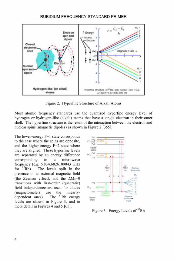
Figure 2. Hyperfine Structure of Alkali Atoms
Most atomic frequency standards use the quantized hyperfine energy level of
hydrogen or hydrogen-like (alkali) atoms that have a single electron in their outer
shell. The hyperfine structure is the result of the interaction between the electron and
nuclear spins (magnetic dipoles) as shown in Figure 2 [355].
The lower-energy F=1 state corresponds
to the case where the spins are opposite,
and the higher-energy F=2 state where
they are aligned. These hyperfine levels
are separated by an energy difference
corresponding to a microwave
frequency (e.g. 6.834.6826109043 GHz
for 87
Rb). The levels split in the
presence of an external magnetic field
(the Zeeman effect), and the MF=0
transitions with first-order (quadratic)
field independence are used for clocks
(magnetometers use the linearly-
dependent ones). The 87
Rb energy
levels are shown in Figure 3, and in
more detail in Figures 4 and 5 [65].
Figure 3. Energy Levels of 87
Rb

PHYSICS
7
Figure 4. 87
Rb D1 Hyperfine Structure

RUBIDIUM FREQUENCY STANDARD PRIMER
8
Figure 5. 87
Rb D2 Hyperfine Structure
PHYSICS
9
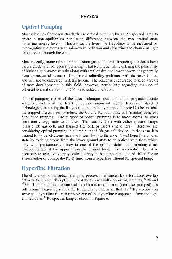
Optical Pumping
Most rubidium frequency standards use optical pumping by an Rb spectral lamp to
create a non-equilibrium population difference between the two ground state
hyperfine energy levels. This allows the hyperfine frequency to be measured by
interrogating the atoms with microwave radiation and observing the change in light
transmission through the cell.
More recently, some rubidium and cesium gas cell atomic frequency standards have
used a diode laser for optical pumping. That technique, while offering the possibility
of higher signal-to-noise ratio along with smaller size and lower power, has generally
been unsuccessful because of noise and reliability problems with the laser diodes,
and will not be discussed in detail herein. The reader is encouraged to keep abreast
of new developments in this field, however, particularly regarding the use of
coherent population trapping (CPT) and pulsed operation.
Optical pumping is one of the basic techniques used for atomic preparation/state
selection, and is at the heart of several important atomic frequency standard
technologies, including the Rb gas cell, the optically pumped/detected Cs beam tube,
the trapped mercury ion standard, the Cs and Rb fountains, and (similar) coherent
population trapping. The purpose of optical pumping is to move atoms (or ions)
from one energy state to another. This can be done with either spectral lamps
(classic Rb gas cell, and trapped Hg ion), or lasers (the others). Here we are
considering optical pumping in a lamp pumped Rb gas cell device. In that case, it is
desired to move Rb atoms from the lower (F=1) to the upper (F=2) hyperfine ground
state by exciting atoms from the lower ground state to an optical state from which
they will spontaneously decay to one of the ground states, thus creating a net
overpopulation of the upper hyperfine ground level. To accomplish that, it is
necessary to selectively apply optical energy at the component labeled “b” in Figure
3 from either or both of the Rb D-lines from a hyperfine-filtered Rb spectral lamp.
Hyperfine Filtration
The efficiency of the optical pumping process is enhanced by a fortuitous overlap
between the optical absorption lines of the two naturally-occurring isotopes, 85
Rb and 87
Rb. This is the main reason that rubidium is used in most (non-laser pumped) gas
cell atomic frequency standards. Rubidium is unique in that the 85
Rb isotope can
serve as a hyperfine filter to remove one of the hyperfine components from the light
emitted by an 87
Rb spectral lamp as shown in Figure 6.

RUBIDIUM FREQUENCY STANDARD PRIMER
10
Figure 6. Isotopic Filtering of 87
Rb D Lines
In this cartoon figure (see Figure 7 for real spectra), the top plot shows the two
hyperfine components in the optical spectrum of one of the 87
Rb D-lines. Because
both hyperfine components are present at equal intensities, this light would be
ineffective for the purpose of optical pumping. The middle plot shows the
absorption spectrum of 85
Rb gas. Notice that the “a” and “A” components overlap
while the “b” and “B” components do not. If the 87
Rb lamp spectrum is passed
through the 85
Rb filter cell, the resulting filtered spectrum is shown in the bottom
plot. The desired “b” component is now significantly larger than the “a” component,
making the filtered spectrum more effective as an optical pumping source for an 87
Rb
absorption cell. The filter cell can be separate or integrated with the absorption
(resonance) cell by using natural Rb with both isotopes.
The D1 line hyperfine spectrum of an actual unfiltered (A) and filtered (B) Rb lamp
is shown in Figure 7 [120]. For optimum performance considering discriminator
signal strength, light shift and temperature coefficient, the desired pumping
component (labeled e,f) is only slightly enhanced.

PHYSICS
11
Figure 7. Unfiltered and Filtered Rb Lamp Spectrum
Passive Atomic Frequency Standards
A passive atomic frequency standard (AFS) is the most common type of atomic
clock. It uses a crystal oscillator or other frequency source to excite a passive atomic
discriminator that produces a correction signal for a frequency control loop to lock
the oscillator to the atomic reference. The crystal oscillator provides the stable
output frequency.
The other type of atomic clock is the active atomic frequency standard, which is an
actual atomic oscillator. The active hydrogen maser is the most common of those,
which excels as the atomic frequency source having the best short term stability. A
passive device is preferred as a primary (absolute) standard (particularly the beam
and fountain devices) because of the ability to evaluate and reduce their bias
corrections and accuracy limitations.
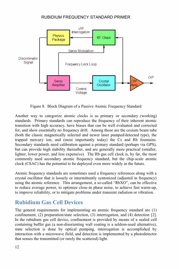
Figure 8 shows the basic block diagram of a passive atomic frequency. The crystal
oscillator excites the physics package through the RF chain, which synthesizes the
nominal atomic frequency. The physics package acts as a passive atomic
discriminator to produce an error signal that is processed by the servo amplifier to
control the frequency of the crystal oscillator. The overall configuration is that of a
frequency lock loop. The discriminator signal is the result of frequency modulation
applied to the RF interrogation, which is synchronously detected by the servo
amplifier to produce the crystal oscillator control voltage. The crystal oscillator
provides the stable output frequency via an output amplifier.
RUBIDIUM FREQUENCY STANDARD PRIMER
12
Figure 8. Block Diagram of a Passive Atomic Frequency Standard
Another way to categorize atomic clocks is as primary or secondary (working)
standards. Primary standards can reproduce the frequency of their inherent atomic
transition with high accuracy, have biases that can be well evaluated and corrected
for, and show essentially no frequency drift. Among those are the cesium beam tube
(both the classic magnetically selected and newer laser pumped/detected type), the
trapped mercury ion, and (most importantly today) the Cs and Rb fountains.
Secondary standards need calibration against a primary standard (perhaps via GPS),
but can provide high stability thereafter, and are generally more practical (smaller,
lighter, lower power, and less expensive). The Rb gas cell clock is, by far, the most
commonly used secondary atomic frequency standard, but the chip-scale atomic
clock (CSAC) has the potential to be deployed even more widely in the future.
Atomic frequency standards are sometimes used a frequency references along with a
crystal oscillator that is loosely or intermittently syntonized (adjusted in frequency)
using the atomic reference. This arrangement, a so-called “RbXO”, can be effective
to reduce average power, to optimize close-in phase noise, to achieve fast warm-up,
to improve reliability, or to mitigate problems under transient radiation or vibration.
Rubidium Gas Cell Devices
The general requirements for implementing an atomic frequency standard are (1)
confinement, (2) preparation/state selection, (3) interrogation, and (4) detection [2].
In the rubidium gas cell device, confinement is provided by means of a sealed cell
containing buffer gas (a non-disorienting wall coating is a seldom-used alternative),
state selection is done by optical pumping, interrogation is accomplished by
interaction with a microwave field, and detection is implemented by a photodetector
that senses the transmitted (or rarely the scattered) light.

PHYSICS
13
Rb Physics Packages
The assembly comprising the atomic frequency reference of an atomic clock is
traditionally called a “physics package”, and a schematic diagram of a generic RFS
physics package is shown in Figure 9.
Figure 9. Schematic of a Classic RFS Physics Package
This figure shows the elements of a classic rubidium gas cell physics package. A
lamp exciter (RF power oscillator) produces a plasma discharge in a small
electrodeless lamp containing 87
Rb, possibly mixed with 85
Rb in a natural or custom
ratio, and an inert buffer gas, usually Xe, sometimes Kr. The output from the lamp
passes through a filter cell containing 85
Rb and another buffer gas, usually N2,
sometimes Ar or a mixture thereof. The filter cell works as a hyperfine optical filter
to improve the optical pumping efficiency. The filtered light then passes through the 87
Rb absorption cell, which also contains a buffer gas, usually N2 or a N2-Ar mixture,
and is located inside a microwave cavity and a C-field coil. The latter makes an
axial DC magnetic field to orient the atoms, separate the Zeeman lines, and (perhaps)
to make fine frequency adjustments. A silicon photodetector senses the light
throughput, producing the output discriminator signal from the physics package,
which is surrounded by one or more high-permeability magnetic shields. The light is
a minimum when the RF excitation applied to the microwave cavity is at the center
of the Rb atomic resonance at 6.835 GHz. The filter and absorption cells may be
separate as shown or combined into a single integrated resonance cell, which
contains a (usually natural) mixture of both Rb isotopes. The lamp, filter (if
separate), and cavity ovens are temperature-controlled. Many aspects of this general
arrangement have been optimized over the years to improve performance, reduce
size, and reduce cost. In particular, the details of the cell sizes, cavity mode, isotopic
and buffer gas mixtures, and oven operating temperatures can improve S/N ratio and
RUBIDIUM FREQUENCY STANDARD PRIMER
14
short-term stability, and reduce sensitivity to temperature, light intensity, and RF
power changes.
Again, the function of the Rb physics package is to produce a discriminator signal
that indicates the frequency of the applied RF excitation. It contains a rubidium
lamp, filter cell and absorption cell in their respective temperature-controlled ovens,
enclosed inside a magnetic shield. The absorption cell oven is also a 6.835 GHz
microwave cavity, and it has a coil to produce a DC magnetic bias field (“C-field”).
The RF power oscillator that excites a plasma discharge in the lamp may be within or
external to the physics package assembly, while a photodiode detects the light
throughput, producing an output signal in response to the applied microwave power.
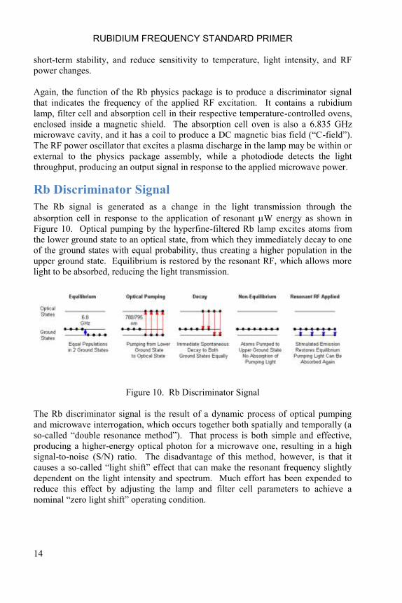
Rb Discriminator Signal
The Rb signal is generated as a change in the light transmission through the
absorption cell in response to the application of resonant W energy as shown in
Figure 10. Optical pumping by the hyperfine-filtered Rb lamp excites atoms from
the lower ground state to an optical state, from which they immediately decay to one
of the ground states with equal probability, thus creating a higher population in the
upper ground state. Equilibrium is restored by the resonant RF, which allows more
light to be absorbed, reducing the light transmission.
Figure 10. Rb Discriminator Signal
The Rb discriminator signal is the result of a dynamic process of optical pumping
and microwave interrogation, which occurs together both spatially and temporally (a
so-called “double resonance method”). That process is both simple and effective,
producing a higher-energy optical photon for a microwave one, resulting in a high
signal-to-noise (S/N) ratio. The disadvantage of this method, however, is that it
causes a so-called “light shift” effect that can make the resonant frequency slightly
dependent on the light intensity and spectrum. Much effort has been expended to
reduce this effect by adjusting the lamp and filter cell parameters to achieve a
nominal “zero light shift” operating condition.
PHYSICS
15
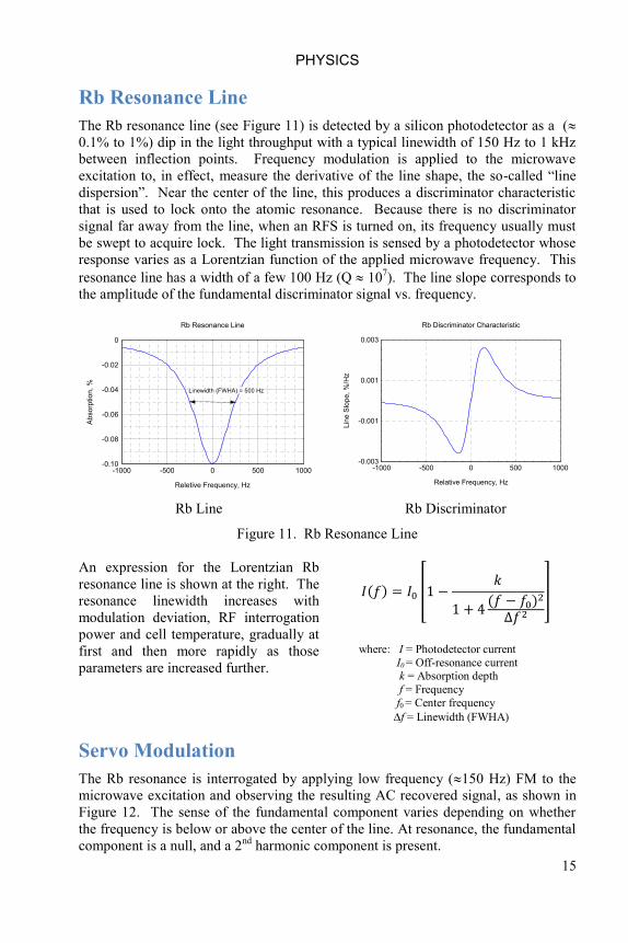
Rb Resonance Line
The Rb resonance line (see Figure 11) is detected by a silicon photodetector as a (
0.1% to 1%) dip in the light throughput with a typical linewidth of 150 Hz to 1 kHz
between inflection points. Frequency modulation is applied to the microwave
excitation to, in effect, measure the derivative of the line shape, the so-called “line
dispersion”. Near the center of the line, this produces a discriminator characteristic
that is used to lock onto the atomic resonance. Because there is no discriminator
signal far away from the line, when an RFS is turned on, its frequency usually must
be swept to acquire lock. The light transmission is sensed by a photodetector whose
response varies as a Lorentzian function of the applied microwave frequency. This
resonance line has a width of a few 100 Hz (Q 107). The line slope corresponds to
the amplitude of the fundamental discriminator signal vs. frequency.
Rb Line
Rb Discriminator
Figure 11. Rb Resonance Line
An expression for the Lorentzian Rb
resonance line is shown at the right. The
resonance linewidth increases with
modulation deviation, RF interrogation
power and cell temperature, gradually at
first and then more rapidly as those
parameters are increased further.
( ) [
( )
]
where: I = Photodetector current
I0 = Off-resonance current k = Absorption depth
f = Frequency
f0 = Center frequency
f = Linewidth (FWHA)
Servo Modulation
The Rb resonance is interrogated by applying low frequency (150 Hz) FM to the
microwave excitation and observing the resulting AC recovered signal, as shown in
Figure 12. The sense of the fundamental component varies depending on whether
the frequency is below or above the center of the line. At resonance, the fundamental
component is a null, and a 2nd
harmonic component is present.
-0.10
-0.08
-0.06
-0.04
-0.02
0
-1000 -500 0 500 1000
Linewidth (FWHA) = 500 Hz
Reletive Frequency, Hz
Ab
so
rptio
n,
%
Rb Resonance Line
-0.003
-0.001
0.001
0.003
-1000 -500 0 500 1000
Relative Frequency, Hz
Lin
e S
lop
e,
%/H
z
Rb Discriminator Characteristic

RUBIDIUM FREQUENCY STANDARD PRIMER
16
Figure 12. Rb Signal Waveforms
When the center frequency is below the center of the resonance line, the light
throughput is higher on one half cycle of the modulation than the other, producing a
fundamental recovered discriminator signal. When the center frequency is above the
center of the resonance line, the light throughput is higher on the other half cycle,
producing a fundamental signal having the opposite polarity. The frequency lock
servo uses the discriminator signal by a process of synchronous detection to steer the
center frequency to the exact center of the resonance line, where the fundamental
component of the discriminator signal is null. At that condition, the square wave FM
modulated RF excitation passes through the center of the resonance line twice per
modulation cycle, producing a second harmonic component. Because the
modulation rate is on the same order as the linewidth, the atomic discriminator acts
like a low-pass filter, changing the square wave FM excitation waveform into a
quasi-sine wave. The second harmonic signal is useful as a means of lock detection,
for monitoring purposes, and to control lock acquisition.
Note that if the square wave FM rate were much lower than the linewidth, the
recovered signal waveform would also be a fundamental square wave of alternating
polarity on each side of resonance, and a null (with transients at the modulation
switching points) at the center. This is the typical response of a cesium beam
instrument.
The frequency lock servo must find the exact center of the atomic resonance with
great precision, e.g., a 10 ppm or -100 dB fundamental null for an offset of 1.5x10⁻¹²
with a symmetric Rb linewidth of 1 kHz. This requires careful avoidance of even-
order modulation distortion, fundamental pickup, and analog offsets.

PHYSICS
17
Modulation Format
RFS designs nearly always use squarewave FM, although sinewave modulation is
occasionally used (e.g., the Stanford Research PRS10, which uses a 12-bit DAC to
synthesize 70 Hz sinusoidal PM), as is squarewave PM (e.g., the
EG&G/PerkinElmer/Excelitas RFS-10, which uses a PLL to inject band-limited
squarewave PM). Squarewave FM can be implemented by either a sawtooth signal
to an analog phase modulator or (preferably) by switching the frequency of a DDS.
Modulation Rate
A relatively fast (in relation to the resonance linewidth) servo modulation rate is used
in most RFS designs to support the fastest possible servo response and thus best
transfer the stability of the Rb reference to locked crystal oscillator [32]. As
mentioned above, this results in a quasi-sinusoidal 2nd
harmonic component in the
recovered signal when the system is in lock at the center of the Rb resonance.
The modulation rate is usually chosen as
the highest convenient value that
maintains a strong discriminator signal,
as shown in Figure 13 where 146 Hz is
used. The squarewave PM modulation
format mentioned above extends that
limit, an advantage for a tactical RFS in
a vibratory environment. The particular
modulation rate is often then selected on
the basis of available values in its
synthesizer that avoid power line
frequencies and other interference.
Figure 13. Signal vs. Modulation Rate
A slow modulation rate does not provide better performance unless a very high
performance crystal oscillator is used, but may be an advantage for digital signal
processing. Slow FM generates a squarewave fundamental signal, and, at the line
center, there is no 2nd
harmonic signal per se but rather transients in response to the
frequency transitions. A DSP servo implementation would blank those out, and can
also use a sampling technique that avoids power line interference. An example of
RFS recovered signals for slow squarewave FM is shown in Figure 14.

RUBIDIUM FREQUENCY STANDARD PRIMER
18
Off Line at Maximum Fundamental At Resonance Line Center
Figure 14. Rb Recovered Signal Waveforms with Slow Squarewave FM
Modulation Deviation
The FM deviation is chosen to
maximize the discriminator slope, and a
typical setting is where the peak
deviation, is equal to the linewidth
between inflection points. Since the
modulation rate is also chosen at about
that value, the FM modulation index,
, is usually about 1.0. The
deviation can be measured by
observing the microwave interrogation
spectrum and noting the difference
between the amplitudes of the carrier
and 1st sidebands (see Figure 15).
Figure 15. FM Modulation Sidebands
Modulation Distortion
Modulation distortion refers to even-order harmonic PM distortion or odd-order AM
distortion applied to the RFS interrogation signal. Either of those results in a
frequency offset and is an important cause of RFS frequency instability. It is easy to
see how AM at the fundamental modulation rate causes a spurious fundamental error
signal component that is synchronously detected like the desired discriminator signal
and produces a frequency offset. The same thing happens to any odd-order AM
component within the preamplifier bandwidth. A similar thing happens as a result of
even-order PM distortion due to an intermodulation effect. For 2nd
harmonic PM
distortion, spurious sideband components are produced at ±2·fmod on the microwave
excitation that mix with the normal fmod modulation to generate a spurious
fundamental recovered signal component that causes a fractional frequency offset
given by
PHYSICS
19
where is the relative amount of 2nd
harmonic distortion and is the Rb line Q.
For -70 dB 2nd
harmonic distortion level and a 300 Hz Rb linewidth ( = 23x106),
the resulting frequency offset is 7x10-12
, and a 15% change in the distortion would
cause a frequency deviation of 1x10-12
. This effect is clearly very important.
Modulation distortion can be caused in several ways: Distortion on the modulation
waveform itself, distortion in the phase modulator, distortion caused by
asymmetrical RF selectivity, and AM-to-PM conversion in the multiplier chain. The
modulation signal itself can be made very pure by generating it from a precise
squarewave followed by passive integration. A low-distortion analog phase
modulator using an all-pass network is discussed below, and it should be applied at a
relatively low RF frequency where the required deviation is small.
Ripple from the fundamental synchronous detector, can reach the VCXO control
voltage even after attenuation by the servo integrator and loop filter. This is mainly
at fmod, which is significant only if it causes AM, but any leakage of 2·fmod is another
cause of even-order modulation distortion.
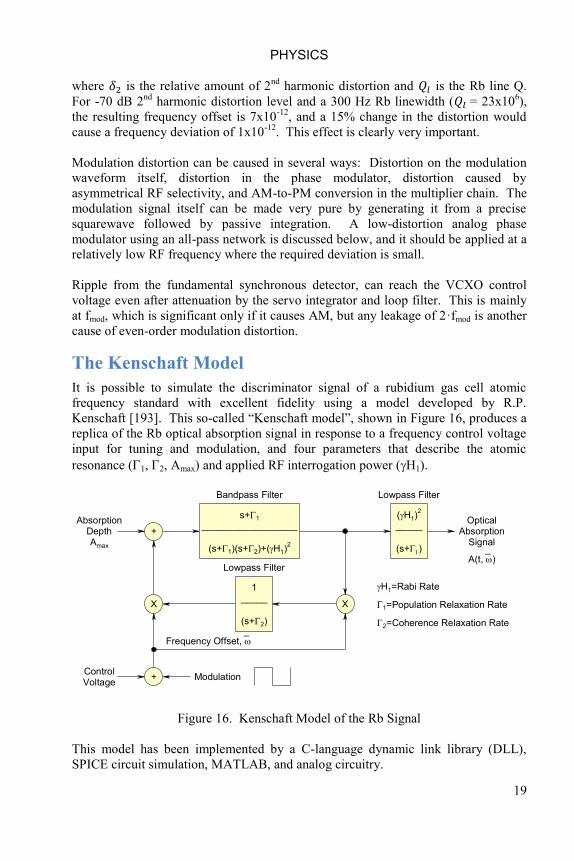
The Kenschaft Model
It is possible to simulate the discriminator signal of a rubidium gas cell atomic
frequency standard with excellent fidelity using a model developed by R.P.
Kenschaft [193]. This so-called “Kenschaft model”, shown in Figure 16, produces a
replica of the Rb optical absorption signal in response to a frequency control voltage
input for tuning and modulation, and four parameters that describe the atomic
resonance (1, 2, Amax) and applied RF interrogation power (H1).
Modulation
OpticalAbsorption
Signal
s+1
__________________
(s+1)(s+2)+(H1)2
1_____
(s+2)
(H1)2
_____
(s+)
+
X
+
X
Bandpass Filter
Lowpass Filter
ControlVoltage
AbsorptionDepthAmax
Lowpass Filter
H1=Rabi Rate
1=Population Relaxation Rate
2=Coherence Relaxation Rate
Frequency Offset,
_A(t, )
_
Figure 16. Kenschaft Model of the Rb Signal
This model has been implemented by a C-language dynamic link library (DLL),
SPICE circuit simulation, MATLAB, and analog circuitry.

RUBIDIUM FREQUENCY STANDARD PRIMER
20
Examples of simulated and actual Rb 2nd
harmonic and fundamental signal
waveforms are shown in Figure 17 [194]. The Kenschaft model is able to very
closely duplicate the actual response.
Figure 17. Simulated and Actual Rb Signal Waveforms
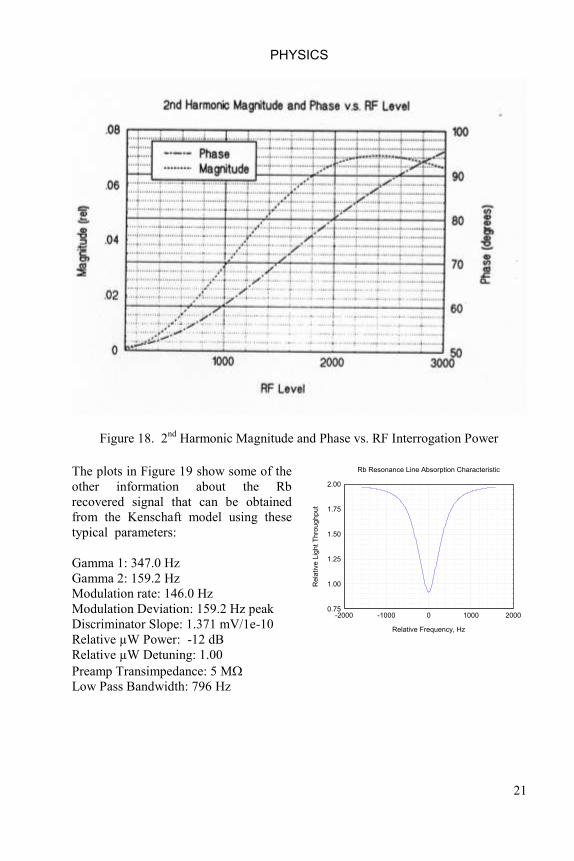
As another example of the utility of the Kenschaft model, it accurately predicts the
magnitude and phase of the recovered 2nd
harmonic signal as a function of the RF
interrogation power (see Figure 18). The predicted sensitivity of the 2nd
harmonic
phase, 0.18º per percent change in RF power, was confirmed by laboratory
measurements. Because it is difficult to directly measure the microwave magnetic
field strength in an operating RFS, this relationship can be of interest for probing the
applied RF power. The Kenschaft model can also be used to predict such
parameters as the 2nd
harmonic phase versus FM deviation, the magnitude and phase
of the fundamental signal versus RF power and the fundamental phase versus FM
deviation.
PHYSICS
21
Figure 18. 2nd
Harmonic Magnitude and Phase vs. RF Interrogation Power
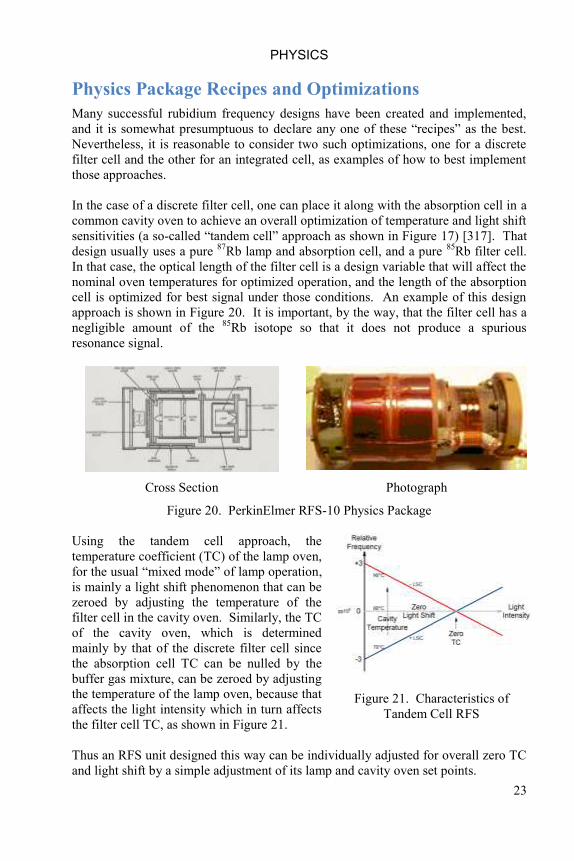
The plots in Figure 19 show some of the
other information about the Rb
recovered signal that can be obtained
from the Kenschaft model using these
typical parameters:
Gamma 1: 347.0 Hz
Gamma 2: 159.2 Hz
Modulation rate: 146.0 Hz
Modulation Deviation: 159.2 Hz peak
Discriminator Slope: 1.371 mV/1e-10
Relative µW Power: -12 dB
Relative µW Detuning: 1.00
Preamp Transimpedance: 5 M
Low Pass Bandwidth: 796 Hz
0.75
1.00
1.25
1.50
1.75
2.00
-2000 -1000 0 1000 2000
Relative Frequency, Hz
Re
lative
Lig
ht
Th
rou
gh
pu
t
Rb Resonance Line Absorption Characteristic

RUBIDIUM FREQUENCY STANDARD PRIMER
22
Figure 19. Rb Signal Plots from Kenschaft Model
0
0.0001
0.0002
0.0003
0.0004
0 400 800 1200 1600
Modulation Deviation, Hz peak
Re
lative
Fu
nd
am
en
tal S
ign
al A
mp
litu
de
Fundamental Signal Amplitude Vs. Modulation Deviation
0
0.04
0.08
0.12
0.16
0 400 800 1200 1600
Modulation Deviation, Hz peak
Re
lative
2n
d H
arm
on
ic S
ign
al A
mp
litu
de
2nd Harmonic Signal Amplitude Vs. Modulation Deviation
0
0.0005
0.0010
0.0015
0.0020
0.0025
-40 -30 -20 -10 0 10
Relative Microwave Power, dB
Re
lative
Fu
nd
am
en
tal S
ign
al A
mp
litu
de
Fundamental Signal Amplitude Vs. Microwave Power
0
0.02
0.04
0.06
0.08
0.10
-40 -30 -20 -10 0 10
Relative Miocrowave Power, dB
Re
lative
2n
d H
arm
on
ic S
ign
al A
mp
litu
de
2nd Harmonic Signal Amplitude Vs. Microwave Power
0
0.0005
0.0010
0.0015
0.0020
0.0025
0 400 800 1200 1600
Modulation Rate, Hz
Re
lative
Fu
nd
am
en
tal S
ign
al A
mp
litu
de
Fundamental Signal Amplitude Vs. Modulation Rate
-0.3
-0.1
0.1
0.3
-2000 -1000 0 1000 2000
Relative Frequency, Hz
Re
lative
Dis
cri
min
ato
r S
ign
al
Discriminator Characteristic
PHYSICS
23
Physics Package Recipes and Optimizations
Many successful rubidium frequency designs have been created and implemented,
and it is somewhat presumptuous to declare any one of these “recipes” as the best.
Nevertheless, it is reasonable to consider two such optimizations, one for a discrete
filter cell and the other for an integrated cell, as examples of how to best implement
those approaches.
In the case of a discrete filter cell, one can place it along with the absorption cell in a
common cavity oven to achieve an overall optimization of temperature and light shift
sensitivities (a so-called “tandem cell” approach as shown in Figure 17) [317]. That
design usually uses a pure 87
Rb lamp and absorption cell, and a pure 85
Rb filter cell.
In that case, the optical length of the filter cell is a design variable that will affect the
nominal oven temperatures for optimized operation, and the length of the absorption
cell is optimized for best signal under those conditions. An example of this design
approach is shown in Figure 20. It is important, by the way, that the filter cell has a
negligible amount of the 85
Rb isotope so that it does not produce a spurious
resonance signal.
Cross Section
Photograph
Figure 20. PerkinElmer RFS-10 Physics Package
Using the tandem cell approach, the
temperature coefficient (TC) of the lamp oven,
for the usual “mixed mode” of lamp operation,
is mainly a light shift phenomenon that can be
zeroed by adjusting the temperature of the
filter cell in the cavity oven. Similarly, the TC
of the cavity oven, which is determined
mainly by that of the discrete filter cell since
the absorption cell TC can be nulled by the
buffer gas mixture, can be zeroed by adjusting
the temperature of the lamp oven, because that
affects the light intensity which in turn affects
the filter cell TC, as shown in Figure 21.
Figure 21. Characteristics of
Tandem Cell RFS
Thus an RFS unit designed this way can be individually adjusted for overall zero TC
and light shift by a simple adjustment of its lamp and cavity oven set points.

RUBIDIUM FREQUENCY STANDARD PRIMER
24
In the case of an integrated resonance cell, the filter and absorption cells necessarily
share the same thermal environment inside the microwave cavity, and its buffer gas
mixture can be chosen for an appropriate TC, which can be adjusted with the lamp
oven temperature because that affects the light intensity and resonance cell TC.
Likewise, the lamp oven TC can be zeroed by the cavity oven temperature. The
nominal light shift condition can be set by adjusting the Rb isotopic ratio in the lamp
[307]. The net result is another optimized design. The only significant disadvantage
of the integrated cell design is that, because of resonance cell inhomogeneity, it has a
significantly larger sensitivity to RF interrogation power than does the separate filter
approach. An example of an integrated cell physics package is shown in Figure 22
[319].
It is worthwhile noting that other forms of inhomogeneity such as a non-uniform C-
field or temperature gradient across the cell can also cause RF power sensitivity, all
of which are aggravated by an uneven microwave interrogation H-field in the region
of the absorption/resonance cell.
13=Feedthru C
14=Cavity & Inner Magnetic Shield
18=Heater Transistor
19b=C-Field Winding
25=Rb Cell
20=SRD
Cross Section Photograph
Figure 22. Symmetricom LPRO Physics Package
Interestingly, the highest performance RFS designs, a family of
EG&G/PerkinElmer/Excelitas GPS satellite clocks, use discrete filter and absorption
cells in separate ovens. In that case, the individual ovens, combined with overall
chassis temperature control, have such high thermal stability that the relatively high
filter cell TC (≈ -6x10-11
/ºC) is not a problem, and the separate filter oven set point
allows precise independent nulling of the light shift.
So there is no single best recipe for an RFS physics package, but all successful
designs have effective ways to minimize TC and light shift sensitivities. For
example, in the GPS Rb clocks mentioned above, they utilize a total absorption cell
buffer gas fill pressure that is chosen for minimum resonance linewidth (highest Q).
In that case, the nominal frequency is a free variable that is adjusted for by the
overall system. An alternative integrated cell space clock design, although not fully
implemented, resulted in a somewhat smaller, lighter and lower physics package
with similar signal parameters, except for an order-of-magnitude larger RF
interrogation power sensitivity.

PHYSICS
25
Rb Lamps
The Rb electrodeless discharge lamp and its RF exciter are important parts of a
rubidium frequency standard. The lamp materials and processing are critical for long
life under the conditions associated with its hot glass envelope and plasma. The
exciter must provide reliable starting and stable running conditions.
Lamp envelope material and Rb fill affect lamp life and noise. Rubidium is lost by
diffusion into the glass under lamp operating conditions, and the key parameters are
glass type, temperature, and excitation power. Too little excess Rb will limit lamp
life, while too much excess Rb can cause noise and instability. A breakthrough for
Rb lamp life (the only important RFS wear-out mechanism) came in the early 1980‟s
with T.J. Lynch‟s idea at EG&G to apply calorimetry to the Rb lamp filling process
[100]. The lamp operates in a temperature-controlled oven at about 120 °C. An RF
power oscillator supplies about 0.5 watt at 130 MHz to excite the lamp. It may be
boosted to assure reliable starting, and must be well-regulated to provide a constant
output spectrum and intensity to avoid frequency changes due to the light shift effect
(frequency versus light intensity). The lamp output is a combination of Rb and
buffer gas spectral lines. In the usual operating mode, the intensity of the Rb
emissions is determined mainly by the Rb vapor pressure (lamp oven temperature),
while the intensity of the buffer gas emissions depend mostly on the exciter RF
power. Thus it is important that the lamp oven temperature be well-controlled to
avoid light shift sensitivity. The lamp output may be passed through a thin-film
optical interference filter to remove most of the useless buffer gas spectral lines so as
to reduce shot noise at the photodetector.
The Rb lamp is the most critical element affecting the life of an RFS physics
package, and it is also important to its frequency stability. Rb lamp life and
reliability considerations are discussed in more detail in the following section. Here
we wish to discuss some of the design considerations that affect successful lamp
operation, particularly those associated with its noise and stability. A drawing [100]
and photograph of a typical Rb lamp is shown in Figure 23.
Drawing of Typical Rb Lamp
Photograph of PerkinElmer RAFS Lamp
Figure 23. Mounted RFS Rb Lamp

RUBIDIUM FREQUENCY STANDARD PRIMER
26
Perhaps the most remarkable characteristic of the small RF-excited electrodeless
spectral lamps used in rubidium frequency standards is their intrinsically low noise.
Lamp noise has negligible influence on the short-term stability of an RFS (in contrast
to the visible flickering of a common neon lamp). Furthermore, the spectral width of
the lamp emissions is ideal in the sense that it provides effective optical pumping
without the need for elaborate wavelength stabilization.
The lamp noise power at the RFS physics package photodetector is effectively shot
noise proportional to the overall light intensity, and recent improvements using
optical filtration limit this noise to the useful Rb D-line emissions. The design issues
related to the Rb lamp (excluding life, see below) therefore center on its reliable
starting and stable running.
Stable lamp running mainly involves the thermal aspects of the Rb lamp, which can
operate in two modes depending on its RF excitation power and temperature (see
Figure 69J). A cold (room temperature) lamp is essentially a buffer gas lamp. The
Rb emissions are small because its vapor pressure is low. As the lamp warms up,
mainly because it is in a heated oven but also because of its excitation power, the Rb
vapor pressure increases and so does the Rb spectral output, principally at the two
deep red 87
Rb D-lines of 780 and 795 nm. That is the normal “mixed-mode”
operating condition, where the lamp emits light at wavelengths associated with both
its buffer gas and rubidium contents. The Rb output is mainly a function of the
temperature (i.e., vapor pressure), while the buffer gas output is mainly a function of
the RF excitation power.
That is the most desirable and stable operating condition, especially if the lamp is
well heat sunk to its thermally-controlled oven. RF excitation power changes mainly
affect the buffer gas output. If the temperature is raised higher, the lamp will enter a
more-intense all-Rb “red mode”, which can provide strong optical pumping and
large signals, but is less stable and (unless attenuated) causes excessive light shift
sensitivity. Furthermore, the region between the mixed and red modes is associated
with gross instability cause by mode hopping and acoustic plasma oscillations
(again, see Figure 69J). An RFS lamp is therefore almost always operated in the
cooler, more stable mixed mode wherein it emits both Rb and buffer gas spectral
lines. In this mode, the Rb light and discriminator signal both increase with a higher
lamp oven temperature and Rb vapor pressure.
With Xe buffer gas, most of the unwanted buffer gas spectral lines can be blocked by
a thin-film optical interference filter, reducing the total light intensity and shot noise
and thereby improving the S/N ratio of the Rb discriminator signal and the overall
short-term stability [154].

PHYSICS
27
Figure 24. Rb Vapor Pressure vs. Temperature
A plot of the 87
Rb vapor pressure versus temperature is shown in Figure 24 [65].
The dashed line denotes the 39ºC melting point. Only a very small amount of Rb
metal is required to maintain a saturated vapor pressure, but excess Rb is needed to
assure long lamp life as it diffuses into the glass lamp envelope. If the initial Rb fill
is insufficient, the lamp will fail prematurely. If the lamp is over-filled, it can
become noisy. Tight process control is therefore necessary on the initial Rb fill.

RUBIDIUM FREQUENCY STANDARD PRIMER
28
Figure 25. Photograph of Temex RFS with Cutaway Physics Package.
The back of the Rb lamp shown in Figure 23 is bonded into a metallic holder to
assure good thermal contact with the lamp oven, and its front portion is inserted into
a coil which couples RF power into it from its lamp exciter, producing a colorful
plasma discharge as shown in Figure 25.
During normal operation, the Rb lamp temperature is well above the melting point of
rubidium, and the molten rubidium must not be allowed to “slosh” around.
Fortunately, for the small amount of excess Rb that is necessary for long lamp life,
surface tension holds it in place under all but the most extreme conditions of shock,
acceleration and vibration. Most importantly, the excess Rb must remain at the
cooler tip of the lamp away from the active discharge region in order to avoid noisy
behavior.
Lamp Life and Calorimetry
The critical factor determining lamp reliability is quantitative control of the lamp Rb
fill and its depletion rate by diffusion into the glass envelope. Tom Lynch of EG&G
effectively solved that problem in 1980 by devising the method of calorimetric Rb
measurement that is now widely used by all organizations making rubidium
frequency standards. By measuring the heat energy required to melt the rubidium in
a lamp, and knowing its heat of fusion, calorimetry provides a nondestructive way to
weigh the Rb in a lamp for manufacturing process control, assessing the initial
“cleanup” due to chemical reactions when the lamp is first ignited, measuring the
rate of Rb depletion as a function of materials (glass type and condition) and
operating conditions (temperature, RF excitation power), and screening lamps for
flight usage, as shown in Figure 26 [120]. Experience shows that it is possible, with
the right design and manufacturing processes, to consistently obtain lamps that have
both low noise and long life. More information about Rb lamp life and calorimetry
will be found in Reference [100].
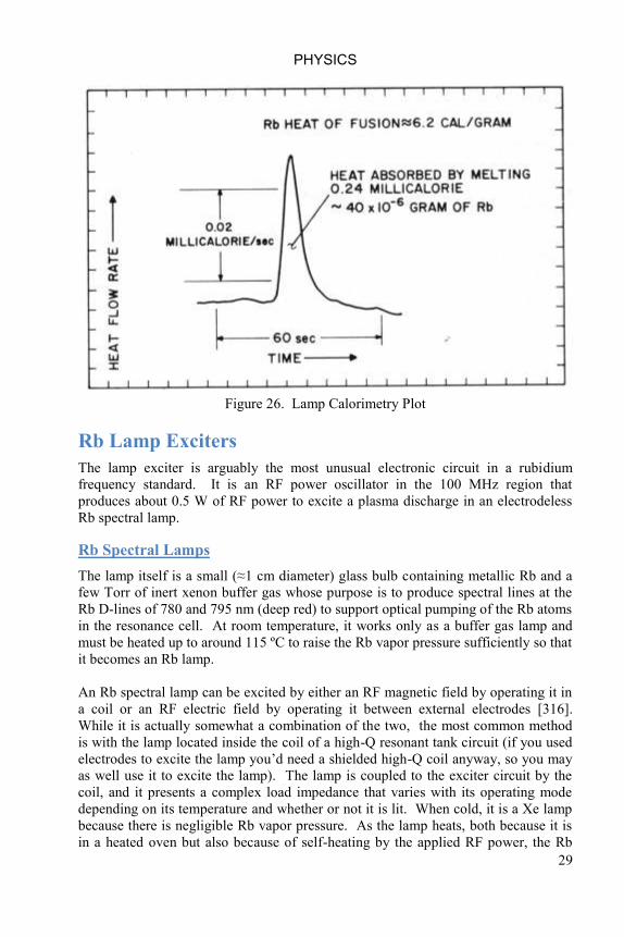
PHYSICS
29
Figure 26. Lamp Calorimetry Plot
Rb Lamp Exciters
The lamp exciter is arguably the most unusual electronic circuit in a rubidium
frequency standard. It is an RF power oscillator in the 100 MHz region that
produces about 0.5 W of RF power to excite a plasma discharge in an electrodeless
Rb spectral lamp.
Rb Spectral Lamps
The lamp itself is a small (≈1 cm diameter) glass bulb containing metallic Rb and a
few Torr of inert xenon buffer gas whose purpose is to produce spectral lines at the
Rb D-lines of 780 and 795 nm (deep red) to support optical pumping of the Rb atoms
in the resonance cell. At room temperature, it works only as a buffer gas lamp and
must be heated up to around 115 ºC to raise the Rb vapor pressure sufficiently so that
it becomes an Rb lamp.
An Rb spectral lamp can be excited by either an RF magnetic field by operating it in
a coil or an RF electric field by operating it between external electrodes [316].
While it is actually somewhat a combination of the two, the most common method
is with the lamp located inside the coil of a high-Q resonant tank circuit (if you used
electrodes to excite the lamp you‟d need a shielded high-Q coil anyway, so you may
as well use it to excite the lamp). The lamp is coupled to the exciter circuit by the
coil, and it presents a complex load impedance that varies with its operating mode
depending on its temperature and whether or not it is lit. When cold, it is a Xe lamp
because there is negligible Rb vapor pressure. As the lamp heats, both because it is
in a heated oven but also because of self-heating by the applied RF power, the Rb

RUBIDIUM FREQUENCY STANDARD PRIMER
30
vapor pressure increases and the Rb atoms, having a lower ionization potential,
absorb more and more of the RF energy, and the lamp enters a mixed Xe-Rb mode.
At even higher temperatures, the lamp will change to a pure Rb mode. Most RFS
operate in the mixed mode at a temperature chosen for optimum Rb spectral output.
That output is controlled mainly by the Rb vapor pressure determined by the
temperature of the well-controlled oven to which the rear of the lamp is thermally
attached. Changes in the RF excitation mainly affect the Xe emission, an advantage
for stable operation. Xe is chosen as the buffer gas for its easiest starting and
because it is possible to remove its unwanted spectral lines by an optical interference
filter [154].
More details about the acceleration of electrons and ions by electric and magnetic
fields, energy gain within a mean free path to cause avalanche breakdown, plasma
temperatures, ion densities and the like will be found in Reference [103].
Lamp Exciters
An RFS lamp exciter is nearly always an RF power oscillator rather than a master
oscillator – power amplifier arrangement because it is essential that the excitation
frequency be aligned with the lamp coil resonance.
There are many RF oscillator circuit
configurations, and many of them have
been used as lamp exciters (early RFS
units used push-pull cross-coupled
vacuum tube oscillators). One of the
most popular is the series-tuned Colpitts
configuration, shown in the basic
schematic of Figure 27. The oscillator
network comprises 150 and 30 pF
capacitors along with the 0.7 µH lamp
coil, series tuned to about 105 MHz by
the 3.6 pF capacitor.
-V
RFC
GHz80239
Rb Lamp
30pF
3.6pF
0.7
H
150pF
Figure 27. Basic Lamp Exciter Circuit
The exciter circuit has to (a) oscillate, (b) start the lamp, and (c) run the lamp. Item
(a) requires that the circuit have sufficient gain to start oscillating at the proper
frequency under all load conditions. Item (b) requires that sufficient RF voltage be
produced to start the plasma discharge. Item (c) involves optimization of the lamp
operating conditions (including its RF excitation power, temperature and temperature
gradients) for best clock performance, and maintaining those conditions indefinitely.
Packaging
One important decision is whether to locate the exciter circuit inside or outside the
lamp oven. The former has the advantages of short leads, smaller packaging, better

PHYSICS
31
EMI containment, higher thermal efficiency and generally better behavior. But it
requires that the exciter transistor operate at the lamp oven temperature. That factor,
and its effect on derating and predicted reliability, can lead to the decision to locate
the lamp exciter outside the lamp oven, connected to it by a short length of coax.
That line is a performance disadvantage, but is an acceptable tradeoff against lower
junction temperature, especially for space applications.
Components
The most important attribute in selecting the RF power transistor is its package. Not
only does it determine its power rating and mounting (an isolated case is much
preferred), but, most importantly it affects the RF circuit layout. More specifically,
multiple low-inductance emitter leads result in better performance and behavior.
The objective is to minimize the destabilizing effect of emitter inductance. No
emitter degeneration resistors are used, both for that reason and to provide the most
gain margin. A lamp exciter using a device with four wide emitter leads each
connected by chip capacitors to adjacent base and collector leads results in excellent
starting and running performance.
The choice between a BJT or MOSFET RF power transistor today is probably a
matter of personal choice. A critical aspect of RF power transistor technology was
the change to all gold metallization systems which solved a long-term metal
migration problem associated with aluminum. A BJT is subject to two main
considerations, base-emitter (B-E) junction breakdown and long-term DC bias
stability. B-E breakdown can cause noisiness and eventual transistor degradation
and failure. It is important therefore to make sure that the RF voltage swings are
within bounds, accomplished mainly by using as large a B-E circuit capacitance as
gain margin allows. The DC bias can be stabilized by an active current regulation
loop [104].
The series capacitor in the lamp network also deserves mention because it must
handle relatively a high RF circulating current and several hundred volts, especially
under starting boost conditions. An ordinary lossy ceramic capacitor will literally
glow cherry red in this circuit. A high quality porcelain RF chip capacitor should be
used, one with a sufficiently high voltage rating.

RUBIDIUM FREQUENCY STANDARD PRIMER
32
Lamp Loading Measurements
It is quite easy to measure the load presented to the exciter circuit by an unlit lamp.
A test fixture can be constructed
consisting of a lamp coil and resonating
capacitor in series, with one end of the
capacitor grounded and other lead from
the coil going to a coaxial connector as
shown in Figure 28. The resonant
impedance of this network can be
measured with a vector impedance meter
or RF network analyzer.
Rs Llamp coil
Cs
Figure 28. Lamp Test Circuit
Without a lamp, the Q is high and the equivalent series loss resistance is about 2.5 ,
corresponding to a Q of about 170. When a lamp in inserted into the coil, the loss
resistance increases, but normally only slightly because the dielectric loss of the
glass is low and the excess Rb is all condensed in the tip of the lamp. The front lamp
holder may be slotted to reduce its shorted-turn loading effect, as seen in Figure 23.
This is the normal starting condition, and the exciter produces a high RF voltage at
the high impedance point where the coil and capacitor connect at the top of the coil
by virtue of the large RF circulating current in the resonant tank. In the case of a
lamp where there is metallic Rb on the exposed inside surface of the lamp, this
conductive layer de-Qs the coil and increases the series load resistance. That can
also be measured in the test fixture, and the worst case loading results is an Rs of 25-
50 . Some loading is also caused by Rb that has diffused into the glass in a lamp
that has operated a long time. This presents the worst case for lamp starting, and
empirical tests are done with “bad” lamps (those that heavily load the coil) and/or by
inserting a physical resistor in series with the coil.
The series LRC lamp network shown in Figure 28 with an added shunt capacitor (the
connector in the test circuit, network capacitors in the oscillator circuit) is the same
as the equivalent circuit for a quartz crystal resonator and many of the same analysis
techniques can be applied, including the use of impedance and admittance circles.
Lamp Exciter Oscillation
A typical lamp exciter oscillates properly with a lamp equivalent resistance of ≈ 50
, and produces a negative resistance of over 200 , which provides a comfortable
margin for its oscillation threshold. Excessive gain can cause spurious oscillation.
Lamp Starting
The details of lamp starting (like so many things when you dig deep enough) are
only partially understood. Clearly electrons and ions are accelerated by the RF
electric and magnetic field excitation until avalanche ionization occurs and the
plasma is lit. But where do the original electrons and ions come from? Cosmic ray

PHYSICS
33
ionization is a leading contender, with natural background radioactivity and the high
energy tail of the buffer gas kinetic distribution being other possibilities. The buffer
gas pressure is optimized for easiest starting. Starting becomes easier as the lamp
heats and the Rb vapor pressure increases because of its lower first ionization
voltage. The coil geometry is another factor that can be optimized experimentally, as
is the lamp position and the details of its holder. Photoionization is very effective in
starting lamps (e.g., a photographic strobe flash or even an electrical spark), but is
not normally necessary. The RF voltage is the most important exciter-related
starting factor.
There isn‟t a lot of information available about long-term lamp starting behavior.
One would assume that starting would become somewhat more difficult for a mature
lamp, but Rb clocks seem to operate properly after years of dormancy without any
problem. Commercial Rb oscillators do get turned on and off more frequently, and
older lamps seem to start fine. The location of the excess Rb in the lamp is a much
more important factor for lamp loading than its long term diffusion into the glass.
Once “chased” into the lamp tip, the excess Rb stays there unless exposed to very
high temperatures (something that does not occur inside a unit). A heavily Rb-
loaded lamp starts if the exciter oscillates and delivers RF power to the lamp. That
power “burns away” the Rb that is loading the exciter by RF induction heating, aided
by the mobility provided by the elevated lamp oven temperature. Even with a well-
chased lamp, a conductive Rb film forms on the inside surface of an unlit lamp that
must be vaporized before it will start, a process that can take a few seconds when
cool. The voltage across the lamp coil gradually increases as the loading decreases
until the lamp starts.
Lamp Running
It is harder to measure the lamp load resistance for an operating lamp. The same test
fixture can be used along with a source of RF power to start and run a lamp (which
will self-heat even if it is not ovenized). But it is difficult to make impedance
measurements in that setup. Passive directional couplers can measure the magnitude
of the forward and reverse power flows. A classic General Radio 1602 passive UHF
admittance meter (Thurston bridge) can provide some information. But the most
practical way to obtain information about an operating lamp exciter is to calculate
the RF current by measuring the RF voltage across a large grounded capacitor. A
small RF current probe can also be used. Circuit voltages can be measured with
built-in peak detector diodes.
Current Regulation
The lamp exciter circuit can includes a regulator that controls the transistor DC bias
current at its nominal during normal operating and at a higher current for starting
boost, controlled by detecting the light [321], [331]. This current regulation provides
several important advantages by (a) stabilizing the lamp exciter DC current during
normal operation, (b) providing a means for boosting the lamp exciter for starting,
(c) maintaining (along with supply voltage regulation) constant DC power input and

RUBIDIUM FREQUENCY STANDARD PRIMER
34
thus stabilizing the RF power delivered to the lamp, and (d) providing additional
attenuation of power supply conducted EMI ripple. Experience from unregulated
BJT lamp exciter circuits in the 1960‟s showed that the DC bias current decreases
significantly over the long term for fixed bias because of transistor β falloff, causing
a drop in lamp power. The current regulator solves that problem, as well as
eliminating the need for individual adjustment. It also avoids changes in DC bias
current caused by radiation exposure. Lamp starting can be aided by boosting either
the exciter supply voltage or its current (or both).
Power Measurements
It is quite easy to measure the RF power delivered to a lamp assembly by a lamp
exciter located outside the lamp oven. One simply uses the lamp oven temperature
controller as a calorimeter by measuring the difference in heater power with the lamp
exciter turned on and off.
Frequency Stability
The lamp exciter frequency is not particularly critical, and it is quite constant
because it is determined mainly by a high quality RF capacitor and a high Q,
temperature-controlled air inductor. The frequency changes several MHz between
the lamp unlit and lit conditions because of non-linear transistor capacitance and
plasma reactance, but that is of little consequence. Little information exists about
long-term lamp exciter frequency change, but it does not appear to be important.
Experience has shown that it is much better to use a tight-tolerance fixed capacitor in
the lamp network rather than a trimmer to adjust the frequency because trimmer
capacitors are very prone to failure, especially in this relatively high-voltage high-
temperature application
Lamp Excitation Power
One would certainly expect that, after some initial stabilization, the lamp excitation
power would naturally tend to decrease over the life of a clock. But most of the
factors involved in such a change (e.g., transistor β falloff) are within the lamp
exciter current regulatory control loop. Thanks to that control loop, most of the
relevant factors can be modeled and analyzed. The main imponderable is the
relationship between DC power input and RF power output delivered to the lamp.
The RF power delivered to the lamp is not itself regulated per se but rather is
determined by the saturation characteristics of the circuit (the supply voltage and
current, transistor limiting, and the oscillator feedback network impedance ratio).
Light Shift
Light shift is the frequency deviation caused by a change in the optical pumping light
intensity or spectrum. It is a fundamental sensitivity of an RFS using the “double-
resonance” method whereby the Rb atoms are simultaneously exposed to pumping
light and RF interrogation. It is easy to understand from a phenomenological

PHYSICS
35
standpoint, but its underlying physics is very complex. Normally one defines it as
the frequency change due to light intensity (i.e., by inserting a neutral density filter in
the light beam), but from a practical engineering standpoint the effect of changing
the lamp oven temperature or the lamp exciter power is more important (those effects
are not identical). Fortunately, the isotopic filter offers an effective way of nulling
the light shift effect, especially if a discrete filter cell is used. In the integrated cell,
light shift, even if nulled from an overall standpoint, causes significant
inhomogeneity that then contributes to RF power sensitivity. In either case, light
shift is a leading candidate for the cause of frequency aging as the properties of the
pumping light change over time.
Pulsed Light
One way, in principle, to eliminate light shift is to operate an RFS in a pulsed mode
whereby the pumping light and the RF interrogation signal are applied sequentially.
Experiments have shown that this is effective to some extent [28] but it raises other
problems having to do with the pulsed operation, and this technique has not found
widespread use, particularly since the isotopic filter is so effective in reducing the
light shift in a more straightforward way.
Isotopic Filter Cells
The ability to improve the optical pumping efficiency with isotopic filtering is a
fundamental advantage of rubidium gas cell frequency standards, some of which use
discrete filter cells for optimum performance. An RFS filter cell is a glass enclosure
containing 85
Rb and an inert buffer gas (e.g., Ar) which is heated to the temperature
where it provides not only enhanced pumping but also a first-order zero light shift
(ZLS) condition.
Absorption Cells
A rubidium gas cell is a glass enclosure containing 87
Rb or natural Rb (72% 85
Rb,
28% 87
Rb) , and an inert buffer gas (e.g. N2, Ar) or a mixture thereof. The cell may
be used alone (a resonance cell) or as an absorption cell with a separate 85
Rb filter
cell. The cell is operated at a stable elevated temperature to establish sufficient Rb
vapor pressure, and the buffer gas prevents wall collisions that would broaden the resonance line. The cell is inside a microwave cavity and is surrounded by a coil to
produce a static DC magnetic field (C-field). The rubidium inside the cell is not
consumed, and lasts infinitely.
The absorption cell is the frequency-determining element in an RFS, and is therefore
a critical aspect of its performance. Besides 87
Rb, it contains a buffer gas to avoid
wall collisions that would otherwise broaden the resonance line (wall coating, a
possible alternative, is seldom used). Two optimum “recipes” have evolved for RFS
physics packages, one for the integrated cell (the more common arrangement), and
another for separate filter and absorption cells. Nitrogen is almost always used
(alone or mixed with argon) as an absorption cell buffer gas because its quenching
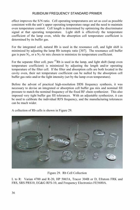
RUBIDIUM FREQUENCY STANDARD PRIMER
36
effect improves the S/N ratio. Cell operating temperatures are set as cool as possible
consistent with the unit‟s upper operating temperature range and the need to maintain
oven temperature control. Cell length is determined by optimizing the discriminator
signal at that operating temperature. Light shift is effectively the temperature
coefficient of the lamp oven, while the absorption cell temperature coefficient is
determined by its buffer gas.
For the integrated cell, natural Rb is used in the resonance cell, and light shift is
minimized by adjusting the lamp Rb isotopic ratio [307]. The resonance cell buffer
gas is pure N2, or a N2-Ar mix chosen to minimize its temperature coefficient.
For the separate filter cell, pure 87
Rb is used in the lamp, and light shift (lamp oven
temperature coefficient) is minimized by adjusting the length and/or operating
temperature of the filter cell. If the filter and absorption cells are both located in the
cavity oven, their net temperature coefficient can be nulled by the absorption cell
buffer gas ratio and/or the light intensity (set by the lamp oven temperature).
Before the advent of practical high-resolution DDS frequency synthesis, it was
necessary to devise an integrated or absorption cell buffer gas mix and nominal fill
pressure to match the nominal frequency of the fixed RF chain synthesizer. This also
imposed very tight buffer gas fill tolerances. With an adjustable synthesizer, it can
be used to calibrate the individual RFS frequency, and the manufacturing tolerances
can be much wider.
A collection of Rb cells is shown in Figure 29.
Figure 29. Rb Cell Collection
L to R: Varian 4700 and R-20, HP 5065A, Tracor 304B or D, Efratom FRK and
FRS, SRS PRS10, EG&G RFS-10, and Frequency Electronics FE5680A.

PHYSICS
37
Early cells had long tubulations to keep condensed Rb out of the microwave cavity
(General Radio did so for that reason and the HP 5065A used thermoelectric cooling
of the cell tip). The Efratom FRK cell has indentations for cavity tuning screws.
The cells in the latest commercial RFS designs have, along with their cavities, gotten
much smaller (see Figure 30). While this comes at the expense of a somewhat
broader line, lower Q and poorer short-term stability, good performance (e.g. y()=
1x10-11
at 1 second) can still be realized. Shorter cells require a higher cell operating
to maintain the same optical absorption and signal strength.
Left:
Symmetricom 8130A Resonance Cell.
Size: 1‟‟ diameter x 1” long
Right:
Symmetricom X72 Resonance Cell
Size: About 0.3” long
Figure 30. Rb Resonance Cells
Cells can be made to operate at higher temperatures by depressing the rubidium
vapor with potassium according to Raoult‟s law.
Cell volumetric change caused by atmospheric pressure variation causes a frequency
deviation because of the buffer gas pressure shift coefficient [68]. This effect scales
with the buffer gas frequency offset, and is primarily due to “oil-can” deflection of
the cell windows. It has a typical value of about 1x10⁻¹⁰
per atmosphere, and can be
an important error budget term for aircraft applications as well as a contributor to a
unit‟s stability floor. Sealed RFS units or physics packages have been used to reduce
or eliminate this effect [159].
All-metal cells have been proposed as a way to (a) eliminate Rb-glass reactions, (b)
eliminate helium permeation, (c) allow high-temperature bakeout, (d) provide precise
filling and sealing, (e) provide low thermal gradients, (f) integrate the cell, cavity and
oven, and (g) support fast warm-up [349]. It is known that rubidium co-exists
happily with copper, which is also an attractive cavity and oven material. Sapphire
windows could be brazed into the cell ends to allow light transmission. The cavity
could extend beyond the cell volume to allow integration of the microwave
multiplier and photodetector. The assembly could use an integrated resonance cell or
incorporate a separate filter cell, and they would be filled via copper tubulations that
would then be pinch sealed. CSAC cells are fabricated from silicon [260].
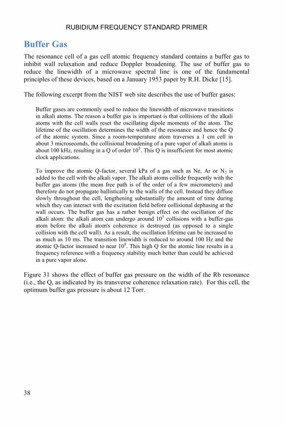
RUBIDIUM FREQUENCY STANDARD PRIMER
38
Buffer Gas
The resonance cell of a gas cell atomic frequency standard contains a buffer gas to
inhibit wall relaxation and reduce Doppler broadening. The use of buffer gas to
reduce the linewidth of a microwave spectral line is one of the fundamental
principles of these devices, based on a January 1953 paper by R.H. Dicke [15].
The following excerpt from the NIST web site describes the use of buffer gases:
Buffer gases are commonly used to reduce the linewidth of microwave transitions
in alkali atoms. The reason a buffer gas is important is that collisions of the alkali
atoms with the cell walls reset the oscillating dipole moments of the atom. The
lifetime of the oscillation determines the width of the resonance and hence the Q
of the atomic system. Since a room-temperature atom traverses a 1 cm cell in
about 3 microseconds, the collisional broadening of a pure vapor of alkali atoms is
about 100 kHz, resulting in a Q of order 105. This Q is insufficient for most atomic
clock applications.
To improve the atomic Q-factor, several kPa of a gas such as Ne, Ar or N2 is
added to the cell with the alkali vapor. The alkali atoms collide frequently with the
buffer gas atoms (the mean free path is of the order of a few micrometers) and
therefore do not propagate ballistically to the walls of the cell. Instead they diffuse
slowly throughout the cell, lengthening substantially the amount of time during
which they can interact with the excitation field before collisional dephasing at the
wall occurs. The buffer gas has a rather benign effect on the oscillation of the
alkali atom: the alkali atom can undergo around 105 collisions with a buffer-gas
atom before the alkali atom's coherence is destroyed (as opposed to a single
collision with the cell wall). As a result, the oscillation lifetime can be increased to
as much as 10 ms. The transition linewidth is reduced to around 100 Hz and the
atomic Q-factor increased to near 108. This high Q for the atomic line results in a
frequency reference with a frequency stability much better than could be achieved
in a pure vapor alone.
Figure 31 shows the effect of buffer gas pressure on the width of the Rb resonance
(i.e., the Q, as indicated by its transverse coherence relaxation rate). For this cell, the
optimum buffer gas pressure is about 12 Torr.

PHYSICS
39
Figure 31. Linewidth versus Buffer Gas Pressure
The following excerpts from P. Bender, et al [220] and W. Stern and R. Novick
[231] describe the effect of a buffer gas on the frequency:
When a rubidium-87 atom collides with a foreign gas molecule, there is an
instantaneous interaction between the dipole moments of the two species. This
interaction can be explained in terms of the attractive van der Waals forces and the
exchange forces and can be considered to cause either an expansion or contraction
of the electronic charge clouds of the interacting species. The change in the
density of the electronic-charge cloud causes a corresponding increase or decrease
in the hyperfine splitting of the ground state of rubidium-87. The van der Waals
forces are long-range attractive forces and always lead to decreases in the
hyperfine separation. For collisions with light buffer gas atoms,, the shift in the
rubidium-87 hyperfine levels is toward higher frequency while for heavy buffer
gas atoms, it is toward lower frequency. The pressure shifts are temperature-
dependent, and the sign of the temperature coefficient tends to be of the same as
the sign of the pressure coefficient.
The buffer gas slightly changes the hyperfine resonance and the resulting frequency
offset is somewhat temperature dependent. The buffer gas pressure shift and
temperature coefficients are nonlinear (they vary with the cell operating
temperature), and their values in the technical literature vary considerably because of
that and other measurement factors. Those values do not appear to depend
importantly on the alkali element (cesium or rubidium) used in the cell. The buffer
gas partial pressure is usually specified at the temperature at which it is filled
(typically +25°C), while the buffer gas pressure shift and temperature coefficients
are usually specified at the temperature at which the cell is operated.
100
200
300
400
500
0 10 20 30 40 50
87Rb Absorption Cell
R=1.2", L=1.6"N
2 + Ar Buffer Gas
Total Buffer Gas Pressure, Torr
Tra
nsve
rse
Re
laxa
tio
n R
ate
,
2,
s-1
Relaxation Rate vs. Buffer Gas Pressure
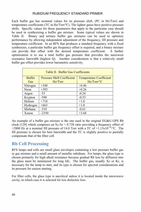
RUBIDIUM FREQUENCY STANDARD PRIMER
40
Each buffer gas has nominal values for its pressure shift, (PC in Hz/Torr) and
temperature coefficients (TC in Hz/Torr/ºC). The lighter gases have positive pressure
shifts. Specific values for those parameters that apply to the particular case should
be used in synthesizing a buffer gas mixture. Some typical values are shown in
Table II. Binary and tertiary buffer gas mixtures can be used to optimize
performance by allowing independent adjustment of the frequency, fill pressure and
temperature coefficient. In an RFS that produces a standard frequency with a fixed
synthesizer, a particular buffer gas frequency offset is required, and a binary mixture
can provide that offset with the desired temperature coefficient. A further
optimization is to use a total buffer gas pressure that provides the narrowest
resonance linewidth (highest Q). Another consideration is that a relatively small
buffer gas offset provides lower barometric sensitivity.
Table II. Buffer Gas Coefficients
Buffer
Gas
Pressure Shift Coefficient
Hz/Torr
Temperature Coefficient
Hz/Torr/°C
Nitrogen +548 +0.46
Neon +392 +0.26
Argon -53 -0.24
Krypton -590 -0.53
Helium +718 +1.0
Hydrogen +663 +1.0
Methane -510 -0.61
Xenon -2350 +3.68
An example of a buffer gas mixture is the one used in the original EG&G GPS Rb
clock [120] which comprises an N2/Ar = 0.728 ratio providing a frequency offset of
+2800 Hz at a nominal fill pressure of 14.0 Torr with a TC of +1.13x10⁻¹⁰
/°C. The
fill pressure is chosen for best linewidth and the TC is slightly positive to partially
compensate that of the filter cell.
Rb Cell Processing
RFS lamps and cells are small glass envelopes containing a low pressure buffer gas
or gas mixture and a small amount of metallic rubidium. For lamps, the glass type is
chosen primarily for high alkali resistance because gradual Rb loss by diffusion into
the glass must be minimized for long life. The buffer gas, usually Xe or Kr, is
necessary for the lamp to start, and its type is chosen for spectral considerations and
its pressure for easiest starting.
For filter cells, the glass type is uncritical unless it is located inside the microwave
cavity, in which case it is selected for low dielectric loss.

PHYSICS
41
For absorption cells, the glass type is selected primarily for low He permeation and
secondarily for low dielectric loss. The absorption cell geometry (dimensions and
wall thicknesses), along with its buffer gas frequency offset, will determine its
barometric sensitivity.
The best Rb ampoules, lamps and cells are processed on ultra-high vacuum systems
and use special processing steps like plasma cleaning to assure the best results.
Ampoules of metallic rubidium are reduced from the chloride under vacuum by
reacting it with barium azide according to the following:
2 RbCl + Ba(N3)2 → 2 Rb + BaCl2 + 3 N2
A typical cell processing setup is shown in Figure 32. The lamp or cell envelopes
are attached to a glass manifold through short tubulations, and the manifold is
connected to vacuum pumps through an isolation valve. The pumps can be a
combination of a sorb pump for roughing and an ion pump for high vacuum. A
previously-prepared Rb ampule is located in a side arm of the manifold along with a
glass-coated magnetic slug used to break it. The system also has a bellows valve for
adjusting its volume, leak and shutoff valves(s) for introducing buffer gas from a
regulated gas bottle, and a high-resolution pressure gauge. The entire system can be
covered with a bakeout hood.
Figure 32. Typical Rb Cell Processing System
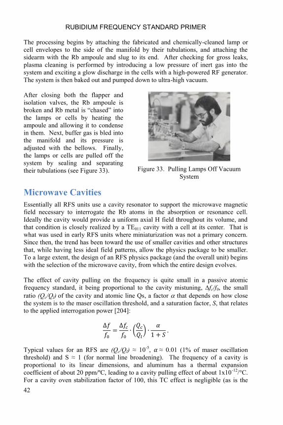
RUBIDIUM FREQUENCY STANDARD PRIMER
42
The processing begins by attaching the fabricated and chemically-cleaned lamp or
cell envelopes to the side of the manifold by their tubulations, and attaching the
sidearm with the Rb ampoule and slug to its end. After checking for gross leaks,
plasma cleaning is performed by introducing a low pressure of inert gas into the
system and exciting a glow discharge in the cells with a high-powered RF generator.
The system is then baked out and pumped down to ultra-high vacuum.
After closing both the flapper and
isolation valves, the Rb ampoule is
broken and Rb metal is “chased” into
the lamps or cells by heating the
ampoule and allowing it to condense
in them. Next, buffer gas is bled into
the manifold and its pressure is
adjusted with the bellows. Finally,
the lamps or cells are pulled off the
system by sealing and separating
their tubulations (see Figure 33).
Figure 33. Pulling Lamps Off Vacuum
System
Microwave Cavities
Essentially all RFS units use a cavity resonator to support the microwave magnetic
field necessary to interrogate the Rb atoms in the absorption or resonance cell.
Ideally the cavity would provide a uniform axial H field throughout its volume, and
that condition is closely realized by a TE011 cavity with a cell at its center. That is
what was used in early RFS units where miniaturization was not a primary concern.
Since then, the trend has been toward the use of smaller cavities and other structures
that, while having less ideal field patterns, allow the physics package to be smaller.
To a large extent, the design of an RFS physics package (and the overall unit) begins
with the selection of the microwave cavity, from which the entire design evolves.
The effect of cavity pulling on the frequency is quite small in a passive atomic
frequency standard, it being proportional to the cavity mistuning, ∆fc/f0, the small
ratio (Qc/Ql) of the cavity and atomic line Qs, a factor that depends on how close
the system is to the maser oscillation threshold, and a saturation factor, S, that relates
to the applied interrogation power [204]:
( )
Typical values for an RFS are (Qc/Ql) ≈ 10-5
, ≈ 0.01 (1% of maser oscillation
threshold) and S ≈ 1 (for normal line broadening). The frequency of a cavity is
proportional to its linear dimensions, and aluminum has a thermal expansion
coefficient of about 20 ppm/ºC, leading to a cavity pulling effect of about 1x10-12
/°C.
For a cavity oven stabilization factor of 100, this TC effect is negligible (as is the

PHYSICS
43
frequency offset compared with the buffer gas offset). Note that this does not
consider the effect of cavity detuning on the interrogation power level along with the
RF power shift coefficient. Nor does it consider the possibility of a stability floor
due to oven temperature set point fluctuations.
The H-field distributions of the near-ideal TE011 and smaller TE111 cavity modes are
shown in Figure 34 (a) and (b) respectively [6]. Note that the optimum position for
the resonance cell is at the center of a TE011 cavity.
The 6.8 GHz microwave cavity of a RFS, more than any other item, determines the
size of the physics package, and much effort has been devoted toward devising small
microwave cavities/resonators having a suitable H-field distribution. The classic
TE011 has an ideal field pattern, but is quite large (the size of a coffee mug) even if
dielectrically loaded, and various smaller TE111 and “magnetron” configurations have
been used. More recently, a significantly smaller capacitively-tuned re-entrant
resonator has been developed for a very small commercial RFS.
The 6.8 GHz microwave cavity of an RFS must provide a reasonably linear and
uniform H-field pattern parallel to the DC magnetic bias (C-field), generally, but not
necessarily, along the optical axis. For a TE011 cavity, the cell is positioned at the
center. For a TE111 cavity, it fills the entire cavity. Only moderate Q (100) is
wanted, to reduce the microwave power requirement without making the tuning
critical. Microwave power is applied to the cavity via an E-probe or H-loop. Non-
uniform microwave magnetic field strength causes signal loss and spatial frequency
differences that produce line broadening and RF power sensitivity. RF power
sensitivity (frequency versus microwave power) is especially important for an
integrated cell, where the frequency has a relatively large spatial variation due to
light shift as hyperfine filtering occurs along the optical path.
The microwave cavity is also a temperature-controlled oven for the
resonance/absorption cell, and it often houses a step recovery diode (SRD)
microwave multiplier. Residual magnetic field from the oven heater must be
minimized to avoid a pseudo temperature coefficient. The C-field coil is generally
wound either on the outside of the cavity or, in the case of a TE111 cavity, directly on
the cell. A temperature gradient is needed to keep the optical path free of condensed
rubidium, but must not be so large as to cause line broadening.
It should be noted that, because of the field reversal in a TE111 cavity, it must be used
either with a buffer gas or a septum to confine the Rb atoms to one region during the
time of an interrogation cycle.

RUBIDIUM FREQUENCY STANDARD PRIMER
44
TE011
Cavity
H-Field
Lines
TE111
Cavity
H-Field
Lines
Figure 34. Cavity Modes
At 6.8 GHz, a TE011 cavity is about the size of a coffee mug, while a TE111 cavity
resembles a “C-size” flashlight battery. Either can hold a 1” diameter by 1” long
typical full-sized cell that operates at around +65°C, in the center of the TE011
cavity or filling the TE111 cavity. The H-field of the TE011 mode is radially
symmetric, but it is asymmetric for the TE111 mode, having two regions of higher H-
field intensity whose orientation is determined by the way the RF current flows
across the ends. A slotted end cap can be used to let light to pass through while
allowing the current to flow. The resonant frequency of an unloaded TE111 cavity is
given by [113]:
√
where f is the frequency in MHz, and D and L are the diameter and length of the
cavity in inches. Some dielectric loading is provided by the cell, and more can be
added to make the cavity smaller.
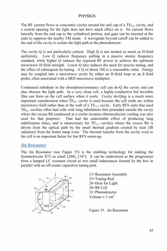
PHYSICS
45
The RF current flows in concentric circles around the end cap of a TE011 cavity, and
a central opening for the light does not have much effect on it. No current flows
laterally from the end cap to the cylindrical portion, and gaps can be inserted at the
ends to suppress the nearby TM mode. A waveguide beyond cutoff can be added to
the end of the cavity to isolate the light path to the photodetector.
The cavity Q is not particularly critical. High Q is not needed as much as H-field
uniformity. Low Q reduces frequency pulling in a passive atomic frequency
standard, while higher Q reduces the required RF power to achieve the optimum
microwave H-field strength. Lower Q also reduces the need for precise tuning, and
the effect of subsequent de-tuning. A Q of about 100 is a reasonable value. Energy
may be coupled into a microwave cavity by either an H-field loop or an E-field
probe, often associated with a SRD microwave multiplier.
Condensed rubidium in the absorption/resonance cell can de-Q the cavity and can
also obscure the light path. In a very clean cell, a highly-conductive but invisible
film can form on the cell surface when it cools. Cavity de-Qing is a much more
important consideration when TE011 cavity is used because the cell walls are within
microwave field rather than at the wall of a TE111 cavity. Early RFS units that used
TE011 cavities often had cells with long tubulations that protruded outside the cavity
where the excess Rb condensed at a cooler location (thermoelectric cooling was also
used for that purpose). That had the undesirable effect of producing long
stabilization times, and is unnecessary for TE111 cavities where the excess Rb is
driven from the optical path by the small thermal gradient created by heat (IR
radiation) from the hotter lamp oven. The thermal transfer from the cavity oven to
the cell is an important factor for fast RFS warm-up.
Jin Resonator
The Jin Resonator (see Figure 35) is the enabling technology for making the
Symmetricom X72 so small [208], [347]. It can be understood as the progression
from a lumped LC resonant circuit to two small inductances formed by the box in
parallel with an off-center capacitive tuning post.
13=Resonator Assembly
23=Tuning Rod
26=Hole for Light
30=Rb Cell
31=Photodetector
Volume 1 cm3
Figure 35. Jin Resonator

RUBIDIUM FREQUENCY STANDARD PRIMER
46
C-Field
An RFS physics package always includes a coil around the absorption or resonance
cell or its microwave cavity to produce a DC magnetic field along the axis of the
microwave H-field that orients the Rb atoms and separates the Zeeman lines so that
the unit locks up on the MF=0, MF=0 transitions with a small quadratic field
dependence. The C-field also provides a means for adjusting the RFS frequency to
correct for cell fill tolerances and frequency drift. Figure 36 shows the RFS C-field
characteristic, f = 573H2, where f is the frequency offset in Hz and H is the magnetic
field in Gauss. A typical C-field coil has a coefficient of 30 mG/mA and is operated
from 50 mG to 300 mG, providing a tuning range of about 7.3x10⁻⁹
. It can, of
course, only raise the frequency.
There are several important advantages of operating an RFS at a minimum C-field
setting of 50 mG, including a relaxation of the magnetic shielding and C-field
stability requirements. That can be made feasible by including provisions for
boosting the C-field during lock acquisition and by using an adjustable synthesizer to
correct for absorption/resonance cell fill tolerances and subsequent frequency drift.
Figure 36. RFS C-Field Characteristic

PHYSICS
47
Advantages of Fixed Minimum C-Field
The quadratic RFS C-field dependence means that the incremental C-field
dependence varies linearly with its nominal value according to the expression (where
H is C-field in Gauss in this and the following equations):
∆f/f = 1.68x10⁻⁷
H ∆H
and the fractional C-field sensitivity therefore varies as H2:
∆f/f = 1.68x10⁻⁷
H2 ∆H/H.
The first equation applies to the case of a small field change (perhaps caused by an
external field), while the second equation describes a fractional C-field change
(perhaps due the TC of the C-field source reference zener). At a nominal C-field of
250 mG, those sensitivities are:
∆f/f = 4.19x10⁻⁸
∆H = 1.05x10⁻⁸
∆H/H.
For example, if an RFS has a magnetic sensitivity specification of 1x10-12
/Gauss, the
C-field can change by no more than 1x10-12
/4.19x10-8
= 24 µG/G, which requires a
shielding factor of about 42,000. Similarly, for a fractional frequency change of
1x10-13
, the C-field must be stable to a factor of at least 1x10-13
/1.05x10-8
= 9.5 ppm.
These requirements can be relaxed by factors of 5 for the shielding factor and 25 for
the C-field stability by operating at the minimum 50 mG C-field value.
C-Field Commutation
The sensitivity of a rubidium frequency standard to external DC magnetic field is
always reduced by surrounding its physics package with magnetic shielding. That
sensitivity can, in principle, be reduced further by symmetrically commutating the C-
field to provide first-order cancellation of the effect of the external field [322].
As stated above, the Rb hyperfine frequency magnetic field dependency is quadratic
according to the relationship:
where is the frequency offset in Hz, and is the magnetic field strength in Gauss.
If is the sum of the applied C-field, , and the residual external (or Earth‟s) field,
, then the frequency offsets for the two directions of the commutated C-field are:
( )
(
) , and
( )
(
),

RUBIDIUM FREQUENCY STANDARD PRIMER
48
and their average is (
).
For the case where the residual external field is small compared with the C-field,
, the term is very small, and the commutated average frequency offset
is approximately equal to the desired undisturbed value:
instead of non-commutated values of
(
) or (
).
For example, for , the additive non-commutated field is 1.21 while the
commutated field is 1.01. Commutation thus provides a significant reduction in the
effect of the external field disturbance (1% versus 21%, in this example).
Unfortunately, it is hard to successfully implement C-field commutation because of
the difficulty of gracefully reversing the direction of current flow through an
inductor (the C-field coil). Transients are produced that degrade the speed and
symmetry of the commutation, and, even more importantly, create unwanted
modulation and interference that impairs RFS operation. Slow commutation
produces unacceptable FM equal to the difference between the two commutated
frequencies, , commutation near or synchronous with the servo
modulation rate produces unacceptable interference with the frequency lock loop,
and fast commutation aggravates the switching transient problems.
Active C-field commutation may have merit in special situations, but it is not a
viable general substitute for adequate passive magnetic shielding in a rubidium
frequency standard.
C-Field Boost During Lock Acquisition
The minimum allowable C-field during lock acquisition is dictated by the accuracy
and tuning range of the crystal oscillator as it is swept to find the Rb resonance. It is
necessary that the C-field be sufficient to prevent lockup on a Zeeman line. The first
order Zeeman lines occur at a separation of ±700 kHz/Gauss, so, for a VCXO with a
tuning range of ±10 ppm, the minimum C-field to assure proper lock acquisition is:
Hmin = 10x10-6
6835x106 / 700x10
3 = 100 mG
If a lower C-field value is desired during normal operation (say 50 mG), then the C-
field should be boosted during lock acquisition.
PHYSICS
49
Magnetic Shielding
An RFS physics package must include magnetic shielding to provide a clean C-field
and to avoid frequency sensitivity from external DC magnetic fields, including the
Earth‟s field of about 0.5 Gauss.
Calculations of magnetic shielding factor are only approximate at best because the
actual geometry is different from that of common equations for the radial attenuation
of infinite nested cylindrical shields. Formulae do exist for calculating the axial
(longitudinal) shielding factor for one or two nested cylindrical shields, but not for
three or more, where only approximate expressions are available. That shielding
factor is higher smaller values of length/radius (L/R). Real RFS shields, even if
nested cylinders, must provide axial attenuation, and are subject to fringing effects at
their ends. They may also have holes and more complex shapes. Shielding formulae
are therefore useful for only first approximations, which can provide insight into
important design variables (e.g., L/R, permeability, annealing process, thickness and
spacing), must yield to empirical measurements to obtain accurate values. An axial
shielding factor of 200,000 is possible with three shields, especially if one of them is
a larger outer case. Modern electromagnetics modeling software may be of some
help. Large shielding factor measurements are often made using low-frequency AC
excitation using a Helmholtz coil to produce a uniform external field and a multi-turn
pickup coil the size and shape of the absorption/resonance cell, perhaps using a lock-
in amplifier as the detector. Those measurements generally correlate well with
actual frequency sensitivity. It is important to measure the shielding at the specified
level external field. RFS magnetic sensitivity is generally measured by observing the
frequency change caused by a reversal of the largest specified field. Besides shield
permeability and thickness, end spacing is particularly critical to avoid reduced
shielding due to fringing. Removable end caps must fit tightly and have generous
overlap, and holes should preferably be at the sides or off-axis. Shields should be
carefully heat treated (annealed) after any machining is done, and handled with care
afterwards. In critical applications, each manufacturing lot should be tested.
Magnetic shield saturation is seldom a problem, but may favor using a lower-
permeability, higher saturation flux material for the outer shield. As its permeability
decreases in a high external field, the inner shields are biased higher and have higher
permeability than their initial value. Obtaining adequate magnetic shielding
becomes increasingly difficult as the overall physics package is made smaller, and it
becomes necessary to use the outer case for that purpose. On the positive side, that
material also serves well to shield against EMI and nuclear radiation. High
permeability tape is sometimes a useful supplement to thicker shields.
Besides passive magnetic shielding, the magnetic field sensitivity of an RFS can be
reduced by (a) operating the unit at low C-field, (b) orienting it that its C-field axis is
orthogonal to the external DC magnetic field, (c) by measuring and compensating for
the external magnetic field by using a magnetic sensor, (d) by occasionally operating
the unit on a Zeeman transition to measure and correct the C-field, or (e) by

RUBIDIUM FREQUENCY STANDARD PRIMER
50
periodically reversing the polarity of the applied C-field (commutation) to eliminate
the quadratic dependence to first order. Method (a) is facilitated by having a high-
resolution synthesizer to make frequency adjustments, method (b) is feasible only in
certain specific cases, method (c) has been implemented with limited success using
Hall-effect magnetic sensors, method (d) has been proven highly effective for a unit
that has microprocessor control and high-resolution frequency synthesis, and method
(e) has also been used, but with limited success.
The innermost RFS magnetic shield is usually close to the C-field winding to
improve its magnetic field uniformity. Any effort to optimize C-field uniformity
must include the effect of magnetic materials in close proximity, including hardware,
electronic devices and heater currents. The latter vary with ambient temperature and
can contribute toward a unit‟s temperature coefficient. A useful diagnostic is to
compare the TC for both C-field polarities. Double-layer, meander-pattern metal foil
heaters with twisted leads have much lower residual field than transistor heaters.
RFS magnetic shields should be degaussed in situ before being used. This can be
done by placing the entire RFS in a solenoidal coil with a series-resonating capacitor
and driving it from the power line via an adjustable autotransformer. The excitation
should be sufficient to saturate the innermost shield and then be slowly reduced to
zero, thereby eliminating residual magnetism.
Photodetectors
Rubidium frequency standards use large
area silicon photodiodes to detect the
light transmission through their physics
packages. A smaller photodetector
would require bulky focusing optics.
Silicon photodiodes have excellent
responsivity at the Rb 780 and 795 nm
wavelengths (see Figure 37), and should
have high shunt resistance (low dark
current) at their operating temperature to
minimize noise, as well as reasonably
low zero-bias capacitance.
Figure 37. Si Photodiode Responsivity
The photodetector shunt resistance determines the amount of noise current that flows
as a result of voltage noise at the input of the preamplifier op amp. It is measured as
the leakage (dark) current that flows when a small reverse voltage is applied across
the junction.
Radiation hardness, particularly responsivity loss in a neutron environment, can also
be a consideration. Neutron bombardment creates lattice defects that cause loss of
photo carriers due to recombination before they can diffuse out of the junction.
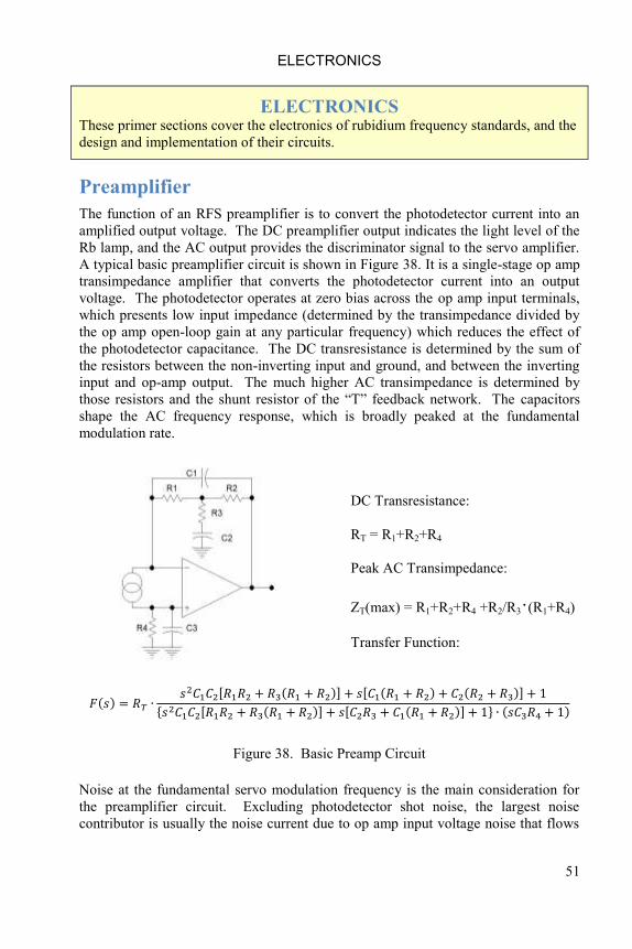
ELECTRONICS
51
ELECTRONICS These primer sections cover the electronics of rubidium frequency standards, and the
design and implementation of their circuits.
Preamplifier
The function of an RFS preamplifier is to convert the photodetector current into an
amplified output voltage. The DC preamplifier output indicates the light level of the
Rb lamp, and the AC output provides the discriminator signal to the servo amplifier.
A typical basic preamplifier circuit is shown in Figure 38. It is a single-stage op amp
transimpedance amplifier that converts the photodetector current into an output
voltage. The photodetector operates at zero bias across the op amp input terminals,
which presents low input impedance (determined by the transimpedance divided by
the op amp open-loop gain at any particular frequency) which reduces the effect of
the photodetector capacitance. The DC transresistance is determined by the sum of
the resistors between the non-inverting input and ground, and between the inverting
input and op-amp output. The much higher AC transimpedance is determined by
those resistors and the shunt resistor of the “T” feedback network. The capacitors
shape the AC frequency response, which is broadly peaked at the fundamental
modulation rate.
DC Transresistance:
RT = R1+R2+R4
Peak AC Transimpedance:
ZT(max) = R1+R2+R4 +R2/R3·(R1+R4)
Transfer Function:
( ) , ( )- , ( ) ( )-
* , ( )- , ( )- + ( )
Figure 38. Basic Preamp Circuit
Noise at the fundamental servo modulation frequency is the main consideration for
the preamplifier circuit. Excluding photodetector shot noise, the largest noise
contributor is usually the noise current due to op amp input voltage noise that flows

RUBIDIUM FREQUENCY STANDARD PRIMER
52
through the photodetector shunt resistance. Other noise sources are the op amp input
current noise and the Johnson noise of the resistors.
S/N Ratio
The dominant noise source in a rubidium gas cell passive atomic frequency standard
is shot noise at the photodetector. Shot noise has a white power spectral density, and
the discriminator signal at the photodetector represents the frequency error, so this
noise corresponds to white FM, and it therefore results in a frequency instability
(Allan deviation) that varies inversely with the square root of the averaging time
[191]. In addition, it is necessary to include a term that represents the contribution of
the phase noise of the RF interrogation signal at twice the servo modulation
frequency that causes additional white FM noise due to an intermodulation effect
[189]. RFS stability is therefore determined by a combination of the signal-to-noise
ratio (S/N), rubidium line Q, and the phase noise of its crystal oscillator according to
the following expression:
( )
( ) √
where Rubidium line Q, full width measured at half amplitude (FWHA).
Rubidium linewidth, maximum signal power, and the photodetector bias current can
all be measured in the laboratory. The signal-to-noise ratio at the output of the
photodetector is defined in a 1-Hz bandwidth as:
( ) = (maximum signal power / shot noise power)1/2
= [(rubidium signal current)2/ (2eI0)]
1/2
where
I0 = photodetector bias current
e = electron charge = 1.6x10⁻¹⁹
coulomb.
Ql is usually measured at normal microwave interrogation power and line
broadening, and a typical value is about 10 million.
The shot noise is caused by the photodetector DC current, which can be calculated
from the preamplifier DC output level and its DC transresistance. A typical value is
50 to 100 µA.
The maximum signal current is calculated based on the peak fundamental rms signal
at the output of the preamplifier and its transimpedance gain at fundamental
frequency.
The contribution to stability due to the VCXO phase noise is discussed in References
[213] and [214]. The second paper indicates that a good estimate of the stability limit
can be made by using the following equation:

ELECTRONICS
53
2
)2(2/1
My
y
fS
where:
Sy(2fM) = Power spectral density of fractional frequency fluctuations at twice the
modulation frequency (fM)
Sy(2fM) is related to the phase noise of the primary loop oscillator by the following
equation:
10/2
2
0
2
2
0
2
102
222
2 MfLMM
MMy
f
ffS
f
ffS
where:
L(2fM) = Phase noise of the primary loop oscillator at twice the modulation rate
fM = Modulation rate
f0 = Nominal VCXO frequency
The two effects combine as the square root of the sum of their squares.
Analog Servo Amplifiers
A typical analog RFS frequency lock servo is shown in Figure 39. The upper
channel processes the fundamental discriminator signal to produce a control voltage
for a VCXO, while the lower channel detects the 2nd
harmonic signal and serves as a
lock detector. A sweep circuit aids lock acquisition.
2fmod fmod
RbSignalFrom
Preamp
Synch DetRef Sigs
ControlVoltageMonitor
VCXOControlVoltage
C-FieldBoost
LockMonitor
Integrator
2nd HarmonicNotch Filter
FundamentalSynchronous
Detector
AcquisitionSweep Circuit
LoopFilter
2nd HarmonicSynchronous
Detector
Lock Detector
Figure 39. Typical Analog Servo Amplifier Block Diagram
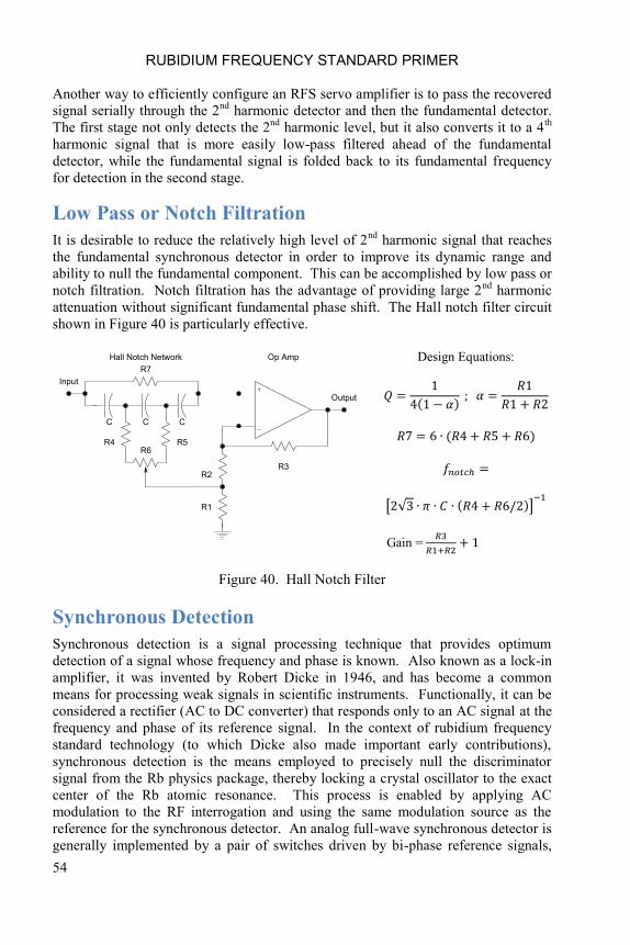
RUBIDIUM FREQUENCY STANDARD PRIMER
54
Another way to efficiently configure an RFS servo amplifier is to pass the recovered
signal serially through the 2nd
harmonic detector and then the fundamental detector.
The first stage not only detects the 2nd
harmonic level, but it also converts it to a 4th
harmonic signal that is more easily low-pass filtered ahead of the fundamental
detector, while the fundamental signal is folded back to its fundamental frequency
for detection in the second stage.
Low Pass or Notch Filtration
It is desirable to reduce the relatively high level of 2nd
harmonic signal that reaches
the fundamental synchronous detector in order to improve its dynamic range and
ability to null the fundamental component. This can be accomplished by low pass or
notch filtration. Notch filtration has the advantage of providing large 2nd
harmonic
attenuation without significant fundamental phase shift. The Hall notch filter circuit
shown in Figure 40 is particularly effective.
R6
R7
Hall Notch Network
C
R4 R5
C C
Input
R3R2
R1
Op Amp
Output
Design Equations:
( )
( )
[ √ ( )]
Gain =
Figure 40. Hall Notch Filter
Synchronous Detection
Synchronous detection is a signal processing technique that provides optimum
detection of a signal whose frequency and phase is known. Also known as a lock-in
amplifier, it was invented by Robert Dicke in 1946, and has become a common
means for processing weak signals in scientific instruments. Functionally, it can be
considered a rectifier (AC to DC converter) that responds only to an AC signal at the
frequency and phase of its reference signal. In the context of rubidium frequency
standard technology (to which Dicke also made important early contributions),
synchronous detection is the means employed to precisely null the discriminator
signal from the Rb physics package, thereby locking a crystal oscillator to the exact
center of the Rb atomic resonance. This process is enabled by applying AC
modulation to the RF interrogation and using the same modulation source as the
reference for the synchronous detector. An analog full-wave synchronous detector is
generally implemented by a pair of switches driven by bi-phase reference signals,

ELECTRONICS
55
and it is sensitive only to an AC input signal at the reference frequency (and its odd
harmonics) having the same phase.
It is important to realize how extremely well the line center must be found. Consider
a GPS Rb clock having a linewidth of 150 Hz at 6835 MHz that realizes a stability of
1x10-14
. The frequency lock loop, and in particular, the fundamental synchronous
detector of the servo amplifier must therefore locate and maintain the frequency to
within 68 µHz, thus “splitting” the resonance line by a factor of about 2 million.
An example of a basic analog synchronous detector circuit is shown in Figure 41.
Figure 41. Basic Synchronous Detector Circuit
This configuration uses shunt FET switches to switch a differential amplifier from an
inverting to a non-inverting configuration in response to the bi-phase reference
signals. Other configurations using series switches and other switch types are
obviously possible. It is critical to keep the reference signals from the synchronous
detector input, and to maintain circuit symmetry in order to avoid offsets and
maintain high quadrature and even harmonic rejection.
A numerical implementation of (perfect) synchronous detection is obviously possible
by appropriately multiplying the signal waveform by +1 or -1.
In an RFS servo, the synchronous detector operates with an integrator to null the
fundamental component of the recovered physics package discriminator signal, the
condition at the center of the Rb resonance line.
Frequency Lock Loop
The frequency lock loop is an essential part of any RFS, and its transfer function
affects its overall stability as described in Reference [213], reproduced in part as
Figure 42 below.

RUBIDIUM FREQUENCY STANDARD PRIMER
56
Figure 42. PSD of Passive Atomic Frequency Standard with Pure Integrator
Frequency Lock Loop
Here, a simple pure integrator is assumed, and the power spectral density (PSD) of
the fractional frequency fluctuations of the locked quartz oscillator that produces the
output signal, Syql(f), 1/Hz, is determined by the PSD of the oscillator, Syq
f(f) and the
PSD of the atomic reference, Syr(f). In addition, it is necessary to include a term that
represents the contribution of the crystal oscillator phase noise at twice the servo
modulation frequency that adds a white FM noise due to an intermodulation effect.
Those factors are analyzed in Reference [214] as excerpted in Figure 43 below:
Figure 43. PSD of Passive Atomic Frequency Standard with General Frequency
Lock Loop
Here the frequency lock servo is characterized by its open-loop (OL) transfer
function, G(s), a typical example of which is shown below, whose configuration
includes a lag-lead filter which is commonly used to allow higher gain at low
frequencies.

ELECTRONICS
57
SynchronousDetector
NotchFilter
5 M x 55 x 0.9
1 uF
Preamp Integrator Lag-LeadFilter
VCXO
50 k
500
47 uF 1.5 ppm/V0.1 s500 pA/1e-10
Physics Package
100 k
Figure 44. Model of RAFS Servo
Figure 44 shows the model for the frequency lock servo. The combination of the
gain blocks is x1860 and the integrator block has a time constant of 0.1 seconds,
resulting in an overall integration characteristic having 0 dB gain at 2960 Hz and a
transfer function G1(s)=18600/s. The lag-lead network with R1=50k, R2=500 and
C=47 µF has a transfer function G2 = (1+Ts)/(1+Ts) where T = R2C = 0.0235
seconds and = (R1+R2)/R2 = 101, with T = 2.37 seconds. This leads to the
overall OL servo transfer function shown in Figure 45.
1m 10m 100m 1 10 100 1k 10k-20
0
20
40
60
80
100
120
Ope
n L
oo
p G
ain
, d
B
Frequency, Hz
Integrator
6.868m
Lag-Lead
30
140
40 dB
300 3k
Figure 45. RAFS Servo Open Loop Gain (Log Approximation)
For good loop stability, the OL servo gain characteristic slope at 0 dB must be about
-6 dB/octave. Thus the overall characteristic is a (not quite pure) integrator with a
-20 dB/decade roll-off plus a lag-lead network seen at the central frequencies as an
increase in the roll-off rate to -40 dB/decade between about 68 mHz and 6.8 Hz that
provides an additional attenuation of -40 dB to stabilize the loop. The closed-loop
(CL) bandwidth is at about 30 Hz and the resulting phase margin is a comfortable
80º.

RUBIDIUM FREQUENCY STANDARD PRIMER
58
Lock Acquisition
An RFS frequency lock loop does not necessarily lock-up on its own, and may need
a specific means of lock acquisition. If the initial VCXO frequency is too far away
from the Rb resonance there may not be sufficient discriminator signal to drive servo
loop into lock. In that case, it is necessary to sweep the frequency until a signal is
detected. Fortunately, that process is quite simple because the servo integrator is
easily made to sweep the VCXO control voltage by injecting an offset current into it,
and the 2nd
harmonic synchronous detector provides a means for indicating lock.
When an RFS is turned on, the VCXO control voltage sweeps until it warms up
sufficiently to produce a discriminator signal. That signal then drives the servo loop
into lock with a frequency offset caused by the integrator sweep injection. Then,
when the signal reaches the lock detector threshold, the sweep is turned off and the
unit operates normally. The whole process is very graceful. In some designs,
especially when fast lockup is required, information from the fundamental detector is
also used to control lock acquisition.
Digital Signal Processing
Digital signal processing (DSP) is increasingly an attractive alternative to an analog
implementation of an RFS servo amplifier [346]. By converting the Rb recovered
signal to numeric form with an analog-to-digital converter, it can be processed
digitally to produce either a VCXO control voltage via a digital-to-analog converter,
or, even better, to directly steer a numerically-controlled oscillator such as a DDS.
Although these techniques are still evolving, they offer the advantage of eliminating
analog errors, better reproducibility, simpler hardware and near-infinite DC gain
since the processing is performed with software rather than analog circuits.
Several hybrid approaches can be taken to evolve from a purely analog to a purely
digital servo amplifier. For example, Figure 46 shows a DSP servo whose front end
uses an analog integrate and dump circuit that acquires information during each half-
cycle of the modulation that is digitized, processed and converted into an analog
control voltage. An important consideration is the need for a high-resolution (e.g.,
20 to 24 bit) DAC. This technique is best applied for relatively slow modulation
rates where there is no large 2nd
harmonic content and the modulation transients can
be suppressed by the reset interval.

ELECTRONICS
59
Integrate& Dump
RbSignalFrom
Preamp
VCXOControlVoltageOutput
Reset
Sample Convert
-
+P DACADC
Figure 46. Integrate and Dump DSP Servo
Figure 47 shows the next step toward DSP where the inputs signal is digitized
directly. In this case, the ADC will acquire multiple samples during each modulation
cycle that are then averaged before further processing. The same high-resolution
DAC requirement applies.
RbSignalFrom
Preamp
VCXOControlVoltageOutput
DACADC P
Figure 47. ADC and DAC DSP Servo
The final step toward an all-digital approach is shown in Figure 48. Here the
oscillator is controlled numerically, eliminating the need for a high-resolution DAC.
The NCO is probably part of a DDS synthesizer.
RFO/P
RbSignalFrom
Preamp
P NCOADC
Figure 48. All Digital DSP Servo
An important consideration in implementing a DSP servo is the modulation rate, i.e.,
whether the recovered signal has a large 2nd
harmonic component due to fast
interrogation (in relation to the atomic resonance linewidth), or whether it more
closely resembles a slower squarewave with a switching transient. Most analog RFS
servos are the former type, and endeavor to implement a fast loop that tightly locks a
VCXO to the atomic resonance. That has important advantages, especially when the
stability of the atomic reference is better than that of the VCXO, and the latter two
RUBIDIUM FREQUENCY STANDARD PRIMER
60
DSP servo schemes are therefore preferred. The DSP software can quite easily
implement signal averaging, synchronous detection and integration, and shaping of
the overall loop response. It can also handle lock acquisition and monitoring, as well
as supporting other more sophisticated processing tasks such as control of the RF
interrogation power and C-field stabilization. Quadrature detection is also quite
easily implemented, which can be used to determine and adjust the detector phasing.
An intermediate implementation can also be effective wherein an analog servo is
controlled by a microcontroller. Digital signal processing can also be employed for
other tasks in an RFS design, including adaptive oven temperature control.
Crystal Oscillators
The crystal oscillator is a key element in an RFS design, particularly since it
determines the unit‟s output phase noise performance beyond the Rb loop bandwidth
and it must also have sufficiently low phase noise, especially at 2·fmod from the
carrier, to drive the internal RF interrogation chain. Its vibration sensitivity is critical
in tactical applications where the combination of passive vibration isolation along
with a fast Rb loop can be an effective solution.
An especially challenging requirement is when the specified phase noise close to the
carrier is better than can be provided by the Rb reference. In that case, a high
performance OCVCXO is necessary along with a slow frequency lock loop. If also
exposed to vibration, a special low g sensitivity crystal oscillator may be required.
RFS crystal oscillators therefore can take several forms. A high stability Rb
reference with a fast servo may use a simple non-ovenized VCXO. More commonly,
a simple VCXO with a temperature-controlled crystal is used, or perhaps the VCXO
shares the physics package cavity oven. Often, the RFS oscillator is at a higher
frequency than its output, which is obtained via frequency dividers. And, as
described above, a high quality OCVCXO may be necessary to provide a low phase
noise output, either as the main RFS source or as separate unit in a secondary phase-
locked loop. In the limit, the overall system may be considered to be an OCVCXO
loosely-coupled to an Rb reference to improve its aging.
Other Oscillators
Some RFS designs use additional oscillators. For example, the RF chain may
include another phase-locked crystal, SAW or DRO VCO to reduce the phase noise
of the microwave interrogation signal.
Transient Response
It must be expected that the quartz crystal resonator of an RFS VCXO will
experience an occasional frequency jump, which will cause a permanent phase error.
For example, a 1x10⁻⁹
VCXO frequency jump would cause a phase error that grows
at the rate of 1 ns per second. For an RFS frequency lock loop that responds within

ELECTRONICS
61
16 ms (a loop bandwidth of 10 Hz), that would cause a time error of only 0.016 ns.
A transient upset of the frequency lock loop itself, without a VCXO or Rb reference
frequency change, will not cause a permanent phase error since the input to the servo
integrator represents frequency, and its VCXO control voltage output represents time
(the integral of frequency), which does not change as long as the loop remains within
its linear range. This is true even if the VCXO frequency requires some finite
amount of time to recover [240]. In contrast, a jump in the Rb reference frequency
causes a permanent frequency change and a corresponding time error that grows with
time.
RF Chains
Many RFS RF chain designs have been successfully implemented as different RF
components have become available. Most start with a requirement to produce a
standard (e.g., 10 MHz) unmodulated RF output, thus requiring some form of
frequency synthesis. Generally, the output signal is derived directly from a VCXO
that is locked to the Rb atomic resonance and determines the phase noise and
spectral purity outside the loop bandwidth. Early RFS RF chain designs were
constrained by the need to use a relatively simple fixed integer (A/B) relationship
between the Rb and output frequencies, thereby determining the absorption buffer
gas offset, and requiring a variable C-field to make frequency adjustments. An
important consideration is the way that their servo modulation is applied, generally
by some form of analog phase modulator. Occasionally, the application does not
require a standard output frequency, and in that case a simpler non-synthesized
approach can be used. More rarely, it is acceptable for the output signal to contain
the servo modulation, which also allows simplification. Modern RF chain designs
can benefit from the availability of direct-digital synthesis (DDS) to support high-
resolution digital frequency adjustment and near-perfect servo modulation. They can
also benefit from the availability of RF components developed for wireless
applications. Note that, as a general principle, one should not use the output of a
DDS as the main source that is multiplied to the Rb frequency, but only as an offset
that is mixed with a pure signal from a crystal oscillator because its phase noise is
relatively high. The following examples show some of the RF chain configurations
that have been used in RFS designs.
Figure 49 shows an example of an RF chain configuration that was popular during
the age of discrete components. It utilizes a simple synthesizer scheme whereby the
Rb frequency is generated by mixing a multiple of 60 MHz (x114 = 6840 MHz) with
5.3125 MHz, which can easily be obtained by mixing 5 MHz with 312.5 kHz (1/16th
of 5 MHz, a particularly favorable binary divisor). The arrangement is further
simplified by using a step recovery diode (SRD) multiplier as the final mixer.
Modulation is applied with an analog phase-shifter near the bottom of the multiplier
chain, and the power of the microwave interrogation signal can be conveniently
adjusted by the level of the 5.3125 MHz component that is simply added to the 60
MHz SRD drive. The disadvantages of this approach are (a) a rather large 4.9 kHz
buffer gas offset, and (b) a microwave spectrum containing many spurious

RUBIDIUM FREQUENCY STANDARD PRIMER
62
components. It is important that the multiplicative contribution to the phase noise on
the interrogation signal comes directly from the pure crystal oscillator. Other early
RFS RF chain designs used a similar arrangement, but incorporated a complex ≈
5.3125 MHz discrete-component synthesizer to allow frequency adjustments and a
lower buffer gas offset. Still other designs of that era used separate multiplier and
balanced mixer assemblies which allowed suppression of the otherwise stronger
carrier component.
RbServo
5 MHz
312.5 kHz
5.3125 MHz
10 MHzO/P
10 MHz 30 MHz 60 MHz
6840 MHz
O/P Amp
Mod SignalfRb
6834.6875 MHz
XO X3 Mod x2SRDx114
2
X
16
X
Figure 49 Classic RFS RF Chain
A modern version of that RF chain is shown in Figure 50, where the fixed 5.3125
MHz section is replaced by a high-resolution DDS that allows fine frequency
adjustments and ideal squarewave FM. Additional advantages of the DDS are that it
can correct for absorption cell frequency tolerances, and that it supports a simple
means for temperature compensation.

ELECTRONICS
63
ModSignal
FreqAdj
+
-
5.3125 MHz Nominal
Use20 MHzClock
32-Bit Resolution:
6.8e-13
SRD Mult & Mxr Part of Rb Physics Pkg
RbServo
60 MHz
10 MHzO/P Amp/Buffer
For 5 MHzO/P
(Sine or Digital)
10 MHzO/P
VCXOSRDx114
X
DDS3
24
fRb
6834.6875 MHz
Figure 50. Modern Tactical RFS RF Chain
Another RFS RF chain arrangement is shown in Figure 51 which offers the
advantage of a cleaner microwave spectrum by avoiding mixing in the SRD
multiplier. A second crystal oscillator is used in a phase-locked loop (PLL) to
generate a pure frequency near 90 MHz at a submultiple of the Rb resonance. In this
scheme, the servo modulation is applied via the PLL. The x9 block is a simple diode
harmonic mixer. Note that the fixed divider could be replaced with a DDS
synthesizer to apply FM and adjust for cell frequency tolerance but, because of the
subsequent x76 multiplication, it would not have sufficient resolution for fine
frequency adjustments.
Rb
Servo
20 MHz
PLL
X969.93 kHz
89.93006993 MHz10 MHz
10 MHz
O/P
Mod
Signal
O/P Amp
XO XO
X
SRD
x762
143
fRb
6834.6853146 MHz
Figure 51. Another Tactical RFS RF Chain
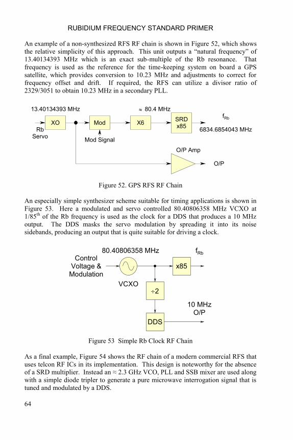
RUBIDIUM FREQUENCY STANDARD PRIMER
64
An example of a non-synthesized RFS RF chain is shown in Figure 52, which shows
the relative simplicity of this approach. This unit outputs a “natural frequency” of
13.40134393 MHz which is an exact sub-multiple of the Rb resonance. That
frequency is used as the reference for the time-keeping system on board a GPS
satellite, which provides conversion to 10.23 MHz and adjustments to correct for
frequency offset and drift. If required, the RFS can utilize a divisor ratio of
2329/3051 to obtain 10.23 MHz in a secondary PLL.
RbServo
13.40134393 MHz 80.4 MHz
O/P
Mod Signal
O/P Amp
fRb
6834.6854043 MHzXO Mod X6
SRDx85
Figure 52. GPS RFS RF Chain
An especially simple synthesizer scheme suitable for timing applications is shown in
Figure 53. Here a modulated and servo controlled 80.40806358 MHz VCXO at
1/85th
of the Rb frequency is used as the clock for a DDS that produces a 10 MHz
output. The DDS masks the servo modulation by spreading it into its noise
sidebands, producing an output that is quite suitable for driving a clock.
80.40806358 MHz
VCXO
10 MHzO/P
fRb
ControlVoltage &
Modulationx85
2
DDS
Figure 53 Simple Rb Clock RF Chain
As a final example, Figure 54 shows the RF chain of a modern commercial RFS that
uses telcon RF ICs in its implementation. This design is noteworthy for the absence
of a SRD multiplier. Instead an ≈ 2.3 GHz VCO, PLL and SSB mixer are used along
with a simple diode tripler to generate a pure microwave interrogation signal that is
tuned and modulated by a DDS.
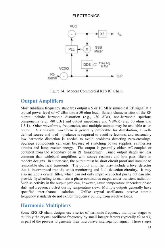
ELECTRONICS
65
Figure 54. Modern Commercial RFS RF Chain
Output Amplifiers
Most rubidium frequency standards output a 5 or 10 MHz sinusoidal RF signal at a
typical power level of +7 dBm into a 50 ohm load. Salient characteristics of the RF
output include harmonic distortion (e.g., -30 dBc), non-harmonic spurious
components (e.g., -80 dBc) and output impedance and VSWR (e.g., 50 ohms and
1.5:1). Other waveforms, frequencies, and multiple outputs may be available as an
option. A sinusoidal waveform is generally preferable for distribution, a well-
defined source and load impedance is required to avoid reflections, and reasonably
low harmonic distortion is needed to avoid problems detecting zero-crossings.
Spurious components can exist because of switching power supplies, synthesizer
circuits and lamp exciter energy. The output is generally either AC-coupled or
obtained from the secondary of an RF transformer. Tuned output stages are less
common than wideband amplifiers with source resistors and low pass filters in
modern designs. In either case, the output must be short circuit proof and immune to
reasonable electrical transients. The output amplifier may include a level detector
that is incorporated into the unit's monitoring and fault detection circuitry. It may
also include a crystal filter, which can not only improve spectral purity but can also
provide flywheeling to maintain a phase-continuous output under transient radiation.
Such selectivity in the output path can, however, cause temperature dependent phase
shift and frequency offset during temperature slew. Multiple outputs generally have
specified inter-channel isolation. Unlike crystal oscillators, passive atomic
frequency standards do not exhibit frequency pulling from reactive loads.
Harmonic Multipliers
Some RFS RF chain designs use a series of harmonic frequency multiplier stages to
multiply the crystal oscillator frequency by small integer factors (typically x2 or x3)
as part of the process to generate their microwave interrogation signal. These stages
RUBIDIUM FREQUENCY STANDARD PRIMER
66
generally use Class C tuned amplifiers or diodes, often in push-push amplifier
doubler, “full-wave rectifier” diode doubler, and Wenzel four diode squarer tripler
configurations [106]. Their tank circuits must have sufficient selectivity to attenuate
sub-harmonics but without excessive tuning sensitivity.
Modulation Distortion
Many subtle modulation distortion effects can occur in a harmonic multiplier chain.
Each stage enhances the PM index while suppressing AM by limiting. AM-to-PM
and PM-to-AM conversions can cause frequency sensitivity to RF stage tuning and
level.
Amplitude modulation on the microwave interrogation signal at the fundamental or
an odd-order multiple of the servo modulation rate will cause a frequency offset and
potential instability because it produces a spurious component on the recovered
signal that the servo nulls by changing the locked frequency. The frequency offset
caused by AM at the servo modulation frequency is given by
where is the relative amount of AM and is the resonance line Q. Similar to 2nd
harmonic PM distortion, a -70 dB AM level with a line Q of 23 million causes a
frequency offset of 7x10-12
.
Sub-Harmonics
The spectrum of a harmonic multiplier chain contains sub-harmonic components that
must be adequately suppressed (e.g., 50 dB or better) before further multiplication to
avoid cyclic phase jitter that causes an interference pattern which can affect the
microwave interrogation power according to the expression
[| ( )|]
where is the change in microwave power in dB, S is the sub-harmonic level in
the drive to the microwave multiplier in dBc and N is its multiplication factor [67].
Phase Modulators
The phase modulator of a traditional RFS RF chain (one that does not use a DDS to
apply servo modulation) is a particularly critical circuit because any amplitude
modulation and even-order distortion it introduces can cause frequency offsets and
instability. Most RFS designs use squarewave FM as their modulation format, which
in an analog RF chain, can be produced by applying triangular PM to a phase
modulator, generally at the lowest frequency of the harmonic multiplier chain where

ELECTRONICS
67
the required deviation is least (a modulation index of ≈1 is required at the Rb
frequency).
A simple R-C low-pass network, where a varactor diode is used as a variable
capacitor, is commonly used, but, at the optimum 45° setting, produces as much AM
as PM. Any such AM can be converted to PM by subsequent circuits, becoming a
source of modulation distortion.
A better approach is to use an all-pass network like that shown in Figure 55. This
all-pass phase modulator suppresses the AM while doubling the modulation
sensitivity, and can therefore provide much better performance (immunity from
subsequent AM-to-PM conversion and lower distortion). The varactor bias is
adjusted for maximum phase sensitivity (≈ -90° where B = G).
.
(a) Basic Circuit
(b) Transfer Function
Figure 55. All-Pass Phase Modulator
Modulation in a phase-locked loop is another possibility but can have problems with
coherent ripple that causes distortion.
Step Recovery Diode Multipliers
Many RFS designs use self-biased high-ratio step recovery diode (SRD) multipliers
to multiply a frequency in the 50-120 MHz range up to the 6835 MHz Rb hyperfine
frequency in one step. This is attractive because of their simplicity, and is feasible
because little microwave interrogation power is needed (typically < 100µW). In
many cases, the SRD multiplier is also used as a mixer. A common configuration is
a 60 MHz to 6840 MHz (x114) multiplier combined with a 5.3125 MHz mixer to
produce an interrogation frequency of 6834.6875 MHz, as shown in Figure 56.
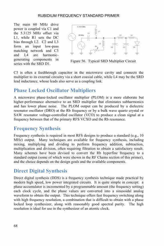
RUBIDIUM FREQUENCY STANDARD PRIMER
68
The main 60 MHz drive
power is coupled via C1 and
the 5.3125 MHz offset via
L1, while R1 sets the DC
bias through L2. C2 and L3
form an input low-pass
matching network and C3
and L4 are harmonic-
generating components in
series with the SRD D1.
Figure 56. Typical SRD Multiplier Circuit
C3 is often a feedthrough capacitor in the microwave cavity and connects the
multiplier to its external circuitry via a short coaxial cable, while L4 may be the SRD
lead inductance, whose leads also serve as a coupling link.
Phase Locked Oscillator Multipliers
A microwave phase-locked oscillator multiplier (PLOM) is a more elaborate but
higher-performance alternative to an SRD multiplier that eliminates subharmonics
and has lower phase noise. The PLOM output can be produced by a dielectric
resonator oscillator (DRO) at the Rb frequency or by a bulk wave quartz crystal or
SAW resonator voltage-controlled oscillator (VCO) to produce a clean signal at a
frequency between that of the primary RFS VCXO and the Rb resonance.
Frequency Synthesis
Frequency synthesis is required in most RFS designs to produce a standard (e.g., 10
MHz) output. Many techniques are available for frequency synthesis, including
mixing, multiplying and dividing to perform frequency addition, subtraction,
multiplication and division, often requiring filtration to obtain a satisfactory result.
Many schemes have been devised to convert the Rb hyperfine frequency to a
standard output (some of which were shown in the RF Chains section of this primer),
and the choice depends on the design goals and the available components.
Direct Digital Synthesis
Direct digital synthesis (DDS) is a frequency synthesis technique made practical by
modern high speed, low power integrated circuits. It is quite simple in concept: a
phase accumulator is incremented by a programmable amount (the frequency setting)
each clock cycle, and the phase values are converted into a sinusoidal analog
waveform to obtain the output. This technique offers fast frequency switching along
with high frequency resolution, a combination that is difficult to obtain with a phase
locked loop synthesizer, along with reasonably good spectral purity. The high
resolution is ideal for use in the synthesizer of an atomic clock.

ELECTRONICS
69
Microwave Spectral Pulling
Spurious spectral components can pull the locked frequency by causing a shift in the
center-of-gravity of the microwave interrogation power. The resulting fractional
frequency change depends on the spurious level and its distance from the carrier
according to the approximate expression [67]
( )
where is the gyromagnetic ratio, B is the spurious microwave induction at
frequency f, and is the center frequency. The pulling can be estimated by scaling
the measured pulling effect of applying a SSB interfering component equal to the
carrier power at some frequency separation, for example, a sideband 5 MHz away
might cause a frequency deviation of 5x10-13
. That would then imply that a -30 dBc
asymmetrical spur from a 25 kHz switching power supply would cause an offset of
1x10-13
.
Oven Temperature Controllers
Oven temperature controllers are a necessary and important part of any RFS design.
The Rb lamp and cells must be heated to obtain sufficient vapor pressure to operate,
and their temperature must be tightly controlled to maintain their stability. These
temperature controllers also influence the unit‟s warm-up and power characteristics.
RFS temperature controllers usually work at DC, but switching controllers are also
used. DC temperature controllers can have their control element (e.g., transistor)
either inside or outside the oven‟s thermal environment. The latter provides greater
efficiency, but raises residual magnetic field issues. A switching power supply has
good efficiency and dynamic range, but introduces EMI concerns.
Most RFS temperature controllers use thermistor temperature sensors because they
are sensitive, small and have reasonably good stability. For good performance, they
must have good thermal contact with their oven, and mechanical stresses must be
avoided.
Some RFS designs use foil heaters with polyimide (Kapton®
) insulation because they
provide good, large-area thermal contact, can have low residual magnetic field and
are very reliable. Two-layer foil heaters with matched meander patterns carrying
opposite currents have very low magnetic field. They can be designed with irregular
shapes and with contacts for thermistor leads. Transistor heaters are efficient and
inexpensive, but have much larger residual field, and necessarily are exposed to high
junction temperatures.
Oven thermal insulation can take many forms, but as RFS ovens have gotten smaller,
there is less need for special insulating materials like urethane foam, and simple

RUBIDIUM FREQUENCY STANDARD PRIMER
70
arrangements like thermally-isolated regions of a printed circuit board can be used.
For space applications, the vacuum environment can be utilized to much advantage.
A typical RFS temperature
controller circuit is shown in
Figure 57. A DC thermistor
bridge senses the oven
temperature and drives a simple
DC proportional controller
comprising a bridge amplifier,
voltage-to-current converter and
heater transistor.
Figure 57. Basic Temperature Controller Circuit
Better performance can be obtained over a wide ambient range with a proportional-
integrator (PI) controller, but it is harder to implement because of the long time
constants that may be involved. Digital temperature controllers are becoming more
common as RFS units include microcontrollers for other purposes. Besides offering
easier implementation of a PI controller, they can also provide adaptive oven demand
power.
The maximum supportable thermal gain can be estimated as the ratio of the oven
thermal time constant to that of either the heater or sensor (whichever is larger).
Thermal stability is improved by a larger oven mass, lower thermal loss, and better
sensor and heater thermal coupling. Elaborate thermal modeling is seldom very
helpful because of the difficulty in obtaining the various parameters, and its limited
effectiveness in predicting gradients. The exact location of the sensor in relation to
ambient is often critical and must be optimized by experiment. Shunting the heater
with an external load to simulate a lower temperature will show the static
proportional gain but tell nothing about the effect of gradients, which can be caused
by asymmetry of the oven, its insulation and lead losses, its heater, and/or any
internal dissipation.
Thermal runaway of an RFS oven is a rare but potentially catastrophic event. Open
thermistor and over-temperature protection may be a wise precaution in some critical
applications.
Mechanical Design
Mechanical design factors are clearly more important in an RFS design than most
types of electronic equipment, mainly because of its physics package. It is useful to
start at the inside of the physics package and consider some of the mechanical,
thermal, structural and magnetic design considerations.
The microwave cavity tends to set the overall size, as well as the size of the
absorption or resonance cell. A smaller cell must operate at a higher temperature to
ELECTRONICS
71
provide a usable Rb signal (i.e., a higher Rb vapor pressure is needed for a shorter
optical length). That may be desirable to support operation in a high-temperature
environment, but it also results in a wider resonance line, lower Q and lower
stability. Nevertheless, very small gas cells work remarkably well, as has been
demonstrated by the mm-sized cells used in chip-scale atomic clocks. For
conventional microwave interrogation, a correspondingly small “cavity” is needed,
which then must either be heavily dielectrically loaded or use a different principle to
produce the required H-field configuration at 6.8 GHz.
For a small design, an integrated resonance cell is almost always used to avoid the
need for a separate filter cell.
Next, one must consider the cell oven, which is also the microwave cavity, and, in
particular the means that heat will be applied. Let us assume that the heating will be
done with DC (AC heating is quite unusual and switching heaters, while offering
good efficiency and dynamic range, create troublesome EMI). A foil heater has
excellent thermal properties and minimal residual magnetic field, but is inefficient if
the control element (e.g., transistor) is located outside the oven. A transistor heater
has 100% efficiency, but applies the heat to a local spot, thus creating poorer
temperature uniformity (gradients) and is likely to create an unacceptable magnetic
field. This leads to the possibility that the cavity oven would be made of a high-
permeability magnetic shielding material, plated for good electrical conductivity (but
still having inferior thermal properties). In that case, the C-field must be inside the
cavity, probably wound on the cell and close to the inner cavity wall.
So our cavity design tends to take one of two approaches, (a) an aluminum oven
shell (copper could also be used for better thermal properties) with a foil heater and
external control element with a C-field coil outside the cavity and magnetic shielding
outside that, or (b) a plated mu-metal oven shell with a transistor heater/control
element with a C-field coil on the cell and additional external magnetic shielding
(perhaps the RFS case).
Let us now consider the lamp oven assembly. It must enclose the lamp and lamp coil
plus its resonating capacitor, but the lamp exciter circuit can be either inside or
outside the lamp oven. If it is inside, its operation is improved because of the short
connections, its power dissipation contributes toward the oven heating, and its EMI
is contained within the oven assembly. But it is a stressful thermal environment, and
a high reliability design is likely to locate the exciter circuit outside the lamp oven.
In that case, it should be as close as possible.
The physics package oven assemblies must be thermally isolated from their
environment but nevertheless ruggedly supported. The performance of their
temperature controllers depends on the oven thermal mass and its thermal loss to
ambient. A space design can effectively utilize vacuum insulation and employ low
emissivity coatings to minimize thermal loss, while a ground-based design can
utilize small air gaps to minimize convective heat transfer. Conductive loss via
RUBIDIUM FREQUENCY STANDARD PRIMER
72
leads, especially coaxial cables, must also be considered. Alloy wire and stainless
steel coax can be used to minimize those losses.
Clearly, there are many interacting considerations that go into an RFS physics
package mechanical design, and all the relevant concerns not have by any means
been exhausted. The need for magnetic shielding must be satisfied by the physics
package and overall structure. The C-field, which is influenced by the magnetic
shielding, must be uniform over the length of the resonance cell to avoid
inhomogeneity, as must thermal gradients be minimized for the same reason.
In a dynamic environment, relative motion between the lamp and cavity assemblies
must be minimized in order to avoid mechanical modulation of the physics package
light path. Mechanical vibration also affects the spectral purity of the crystal
oscillator and thereby the microwave interrogation signal, and vibration isolation
may be required. Fortunately, a wide bandwidth Rb servo can reduce vibration
sensitivity at the lower vibration rates, so the vibration isolators need work only at
higher, more practical, vibration frequencies. Cable isolators, although large, have
been found to be particularly effective, but may inhibit thermal transfer.
RFS modules have few, if any, physical controls. Older units had accessible
potentiometers for adjusting their frequency, but nowadays that is more likely to be
accomplished with an external voltage or resistance, or an internal non-volatile
digital memory. Some units have a lock indicator, and none have on-off switches.
All RFS modules have a connector for DC power, analog monitor signals and,
possibly, digital control lines. The same connector may contain the RF output
signal, or otherwise it will have a separate coaxial connector. Dual RF outputs are
sometimes available, possibly at different frequencies.
Complete RFS instruments are far less common, and have a larger complement of
connectors, indicators and controls, and generally operate from the AC power mains.
Thermal Design
In general, conductive heat transfer is preferred, and is essential for vacuum
operation. Temperature gradients should be minimized in the overall RFS chassis as
well as in its physics package ovens, because, in air, they may cause frequency
changes that depend on the orientation of the unit (otherwise an RFS frequency is not
sensitive to static g forces or tip-over).
Small RFS units often dissipate enough power that they must be heat sunk in some
way, making them not so small after all.
Baseplate Temperature Control
Baseplate temperature control can be used to stabilize the chassis temperature of an
RFS against environmental temperature variations. For example, a GPS satellite Rb

ELECTRONICS
73
clock may have an integral baseplate temperature controller (BTC) comprising
heaters and a thermistor temperature sensor inside the bottom of the RFS chassis, a
thermal insulator between the chassis and the space vehicle (S/V) panel, and an
electronic controller circuit. Besides improving the RFS stability, the BTC also has
the advantage of allowing its performance testing and operation to be limited to a
single temperature. Its main disadvantage is an increase in power consumption that
depends on the difference between the BTC set point and S/V panel temperatures.
An example of BTC operation is shown in Figure 58, which plots its overall power
consumption against the S/V panel temperature to which it is mounted.
The BTC set point is +45°C, where the
total power is zero, but the hottest
possible operating condition is when
the S/V panel is at +25°C, where the
BTC heater power is zero but the clock
itself still dissipates 14 watts.
Similarly, the coldest possible
operating condition is when the S/V
panel is at -11°C and the heater is at its
maximum demand power. The slope
of this operating characteristic is
determined by the 0.7 W/°C thermal
conductance of the thermal insulator.
Figure 58. BTC Thermal Characteristic
An uncontrolled RFS with a temperature
coefficient of 2x10-13
/ºC, would show
significant instability when exposed to
12-hour orbital S/V panel temperature
variations of 3.5°C peak-peak, as shown
in the Figure 59. The BTC reduces this
instability about two orders-of-
magnitude to below the 2x10-12
-1/2
+2x10-14
noise level of this example.
Figure 59. Stability Plot for RFS Under
Temperature Cycling without BTC
Stability
Frequency stability is the main attribute of a rubidium frequency standard, so it
naturally follows that it plays an important role in their design, specification and
testing. RFS stability (actually instability) is usually separated into its noise-like
frequency fluctuations, its gradual frequency change over time, and the dependence
of its frequency on environmental factors such as temperature and supply voltage. It
RUBIDIUM FREQUENCY STANDARD PRIMER
74
is best that those sources of instability be examined separately. The noise-like
frequency fluctuations are described by statistical stability measures, the frequency
aging is usually described under constant environmental conditions, and the
environmental sensitivity is expressed by a number of individual sensitivities. Note
that aging refers to internal RFS mechanisms that cause its frequency to change
while drift includes external factors and therefore depends on the unit‟s operating
conditions. This primer section emphasizes the measurement and analysis of the
noise-like frequency fluctuations, which are commonly described by power-law
power spectral densities ranging from white PM to flicker FM noise. As we have
seen previously, the dominant RFS noise type is white FM noise extending over
averaging times from 1 second to several hours or more.
Stability Measures
The principal RFS time-domain stability measure is the Allan deviation which is a
statistic similar to the ordinary standard deviation but is better able to handle the
more divergent noise sources that are present in most frequency sources [255], [354].
In the frequency domain, the stability of an RFS can be described by its phase noise.
Those two methodologies are complementary. Time domain measures are generally
applied for analyzing stability at times of 1 second and longer while frequency
domain measures are more often used for shorter averaging times. Conversions are
possible between the two domains, but it is usually best to use the one that most
closely resembles the requirements of a particular application.
Stability Measurements
RFS stability measurements generally require greater precision and accuracy than
can be obtained from an ordinary frequency counter [358]. High precision can be
achieved by a heterodyne process that enhances the measurement resolution, while
high accuracy requires a suitable reference source such as a cesium beam instrument
or a GPS time and frequency receiver. RFS stability is best performed by measuring
its phase, from which data it is easy to also obtain its frequency record.
Stability Analysis
The stability of an RFS is usually analyzed in a series of steps designed to separate
and describe both its deterministic and stochastic behavior, while dealing with any
anomalies involving the measurements or unit under test.
One usually begins with a phase record, its time error versus a highly stable
reference. Because an RFS has high stability (pp1013
) but is likely to have a rather
large frequency offset (pp1010
) and significant frequency drift (pp1012
/day), the raw
phase record may be a straight line whose slope corresponds to the frequency offset.
So the next steps in the analysis process are to remove that frequency offset and drift,
which we assume are deterministic parameters.

ELECTRONICS
75
The following example (see Figures 60-67) shows the basic RFS stability analysis of
a 1-week set of = 1 second simulated phase data having a nominal frequency offset
of 1x10⁻¹⁰
, white FM noise at a level of 1x10-11
-1/2,
and linear frequency drift of
3x10-12
/day.
The phase data are essentially a straight
line whose slope represents the average
frequency offset (1.035x10⁻¹⁰
), which
can be determined by a least-squares
linear fit. If that were removed from the
phase data, one would see a quadratic
representing the frequency drift as
shown in Figure 61. If a quadratic fit
were removed from the phase data, one
would see phase residuals showing their
noise fluctuations as shown in Figure 62.
Figure 60. Phase Data
Figure 61. Phase Residuals
without Frequency Offset
Figure 62. Phase Residuals
without Frequency Offset Drift
Converting the original phase data to
frequency data shows that there is linear
frequency drift plus noise. Note that if
there were outliers in the frequency data
they would have to be removed before
proceeding with the analysis. The drift
can be made clearer by averaging the
frequency data as shown in Figures 64
and 65 for averaging factors of 10 and
100 respectively.
Figure 63. Frequency Data

RUBIDIUM FREQUENCY STANDARD PRIMER
76
Figure 64. Frequency Data
Averaged by Factor of 10
Figure 65. Frequency Data
Averaged by Factor of 100
Removing a linear fit from the frequency
data leaves the frequency residuals
which can then be analyzed for their
noise.
Figure 66. Frequency Residuals
An Allan deviation plot shows the
frequency stability versus averaging
time. The white FM noise has a slope of
-0.5 on a log sigma versus log tau plot.
Note that most RFS units would have
flicker FM noise that would impose a
noise floor before the stability reached
1x10-13
. Other statistics are available to
analyze frequency stability for data
having linear drift, with better
confidence and at larger averaging
factors [354].
Figure 67. Frequency Stability
It is important to inspect the phase and frequency records for jumps and other
anomalies. The source of a phase discontinuity is unlikely to be in the frequency
standard, but rather a problem with the measuring system, but nevertheless should be
explained. A frequency jump is potentially a serious problem for a frequency
standard and requires careful investigation.
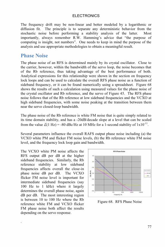
ELECTRONICS
77
The frequency drift may be non-linear and better modeled by a logarithmic or
diffusion fit. The principle is to separate any deterministic behavior from the
stochastic noise before performing a stability analysis of the latter. Most
importantly, always remember R.W. Hamming‟s advice that “the purpose of
computing is insight, not numbers”. One needs to keep in mind the purpose of the
analysis and use appropriate methodologies to obtain a meaningful result.
Phase Noise
The phase noise of an RFS is determined mainly by its crystal oscillator. Close to
the carrier, however, within the bandwidth of the servo loop, the noise becomes that
of the Rb reference, thus taking advantage of the best performance of both.
Analytical expressions for this relationship were shown in the section on frequency
lock loops and can be used to calculate the overall RFS phase noise as a function of
sideband frequency, or it can be found numerically using a spreadsheet. Figure 68
shows the results of such a calculation using measured values for the phase noise of
the crystal oscillator and Rb reference, and the servo of Figure 45. The RFS phase
noise follows that of the Rb reference at low sideband frequencies and the VCXO at
high sideband frequencies, with some noise peaking at the transition between them
near the servo closed-loop bandwidth.
The phase noise of the Rb reference is white FM noise that is quite simply related to
its time domain stability, and has a -20dB/decade slope at a level that can be scaled
from the value L(1 Hz) = -80 dBc/Hz at 10 MHz for a 1-second stability of 1x10-11
.
Several parameters influence the overall RAFS output phase noise including (a) the
VCXO white PM and flicker FM noise levels, (b) the Rb reference white FM noise
level, and the frequency lock loop gain and bandwidth.
The VCXO white PM noise affects the
RFS output dB per dB at the higher
sideband frequencies. Similarly, the Rb
reference stability at low sideband
frequencies affects overall the close-in
phase noise dB per dB. The VCXO
flicker FM noise level is important for
intermediate sideband frequencies (say
100 Hz to 1 kHz) where it largely
determines the overall phase noise, again
dB per dB. The most interesting region
is between 10 to 100 Hz where the Rb
reference white FM and VCXO flicker
FM phase noise both affect the results
depending on the servo response.
Figure 68. RFS Phase Noise
.

RUBIDIUM FREQUENCY STANDARD PRIMER
78
Note that this model does not include an explicit SyN(f) term for the 2fmod
intermodulation noise because that is already included in the white FM noise values.
Signal Parameters
An RFS physics package is characterized by a number of parameters that describe
the dependence of its linewidth, discriminator signal and light shift to such operating
conditions as lamp, filter cell and absorption cell temperatures, RF interrogation
power, modulation rate and deviation. Figure 69 shows some of these dependencies
in the form of plots from research conducted during the development of the EG&G
GPS Rb clocks [30]. While they apply to that particular hardware and its operating
conditions, they also serve to show the general dependences of an RFS physics
package using a discrete filter cell. The plots are not necessarily from the same cells
or operating conditions, and should not be used for quantitative comparisons, but
illustrate the sort of investigations that are performed during RFS development. The
following notes describe some of the features of the individual plots:
A. The linewidth increases with modulation deviation and RF interrogation power
due to line broadening
B. The linewidth increases with RF power and the signal peaks at a particular RF
power. There is an optimum RF interrogation power as a tradeoff between
signal strength and RF broadening.
C. The linewidth increases at higher temperatures due to an increase in Rb vapor
pressure and a higher spin-spin collision rate.
D. The frequency decreases with filter cell temperature in the region where the
signal is strongest. All RFS have a relatively large negative filter cell TC under
their normal operating conditions.
E. The lamp TC is a light shift effect that can be nulled by adjusting the filter cell
temperature (or length).
F. This shows the desired zero light shift condition at the optimum filter cell
temperature.
G. This is the actual light shift coefficient, showing the null (flat line) at the
optimum filter cell temperature, and that the lines converge at zero light
intensity.
H. The signal peaks at a particular light intensity due to light broadening above that
point, and at a higher than optimum filter cell temperature.
I. The cell TC is determined mainly by its buffer gas mixture (N2/Ar=0.73 here)
and is non-linear.
J. The lamp modes depend on both temperature and RF excitation power (lamp
exciter supply voltage here). The two basic modes are called “ring” and “red”
based on their appearance, and there is an oscillatory region between them,
along with considerable hysteresis. Most RFS operate in the cooler ring mode,
which avoids the oscillatory region, because, although the brighter red mode
signal is stronger, the light shift is larger and the spectral lines are self-reversed.

ELECTRONICS
79
A. Linewidth vs. Modulation Deviation
B. Linewidth and Signal vs. RF Power
C. Linewidth vs. Cell Temperature
D. Frequency and Signal vs. Filter
Temperature
Figure 69. RFS Signal Parameters

RUBIDIUM FREQUENCY STANDARD PRIMER
80
E. Frequency vs. Lamp Temperature
F. Light Shift Coefficient vs. Filter
Temperature
G. Frequency vs. Light Intensity
H. Signal vs. Lamp Temperature
Figure 69. RFS Signal Parameters (Cont.)

ELECTRONICS
81
I. Frequency vs. Cell Temperature
J. Lamp Modes
Figure 69. RFS Signal Parameters (Cont.)
RFS Internal Operating Adjustments
An RFS requires several of its operating parameters to be adjusted for best
performance depending on its particular design and the degree to which it is to be
individually optimized. Those adjustments and parameters may include some or all
of the following:
1. Frequency calibration
2. RF interrogation power
3. Oven temperature set points
4. Modulation deviation
5. Synchronous detector phasing
6. Lamp exciter frequency
7. Internal temperature compensation
8. S/N and S/W version information
Commercial units generally minimize such adjustments to save manufacturing cost,
militarized units are generally subjected to more extensive testing during which
certain adjustments may be made, and space units generally emphasis performance
and undergo extensive acceptance testing and optimization.
Frequency calibration is almost always done, either by adjusting the C-field or the
setting of a frequency synthesizer. It is usually necessary to adjust the RF
interrogation power, especially if a SRD multiplier is used whose DC bias very
likely requires adjustment. Oven temperatures, which affect important operating
parameters like light shift and TCs, may be individually set. Modulation deviation
often requires adjustment if it is implemented with an analog phase modulator rather
than a DDS. An adjustment of the lamp exciter frequency is generally not required,
nor is adjustment of the synchronous detector phasing. If internal temperature

RUBIDIUM FREQUENCY STANDARD PRIMER
82
compensation is used, it likely must be individually set. An RFS with digital control
requires that its embedded software be loaded, and generally includes specific serial
number and version information.
Internal Measurements
Several techniques have been found useful for measuring internal RFS operating
parameters.
1. The physics package discriminator signal is its primary attribute, but is not
directly observable during normal operation. The 2nd
harmonic signal is
therefore often used as a proxy for it while making internal adjustments and to
judge the general health of a unit. Measuring the actual discriminator slope, the
amount of fundamental recovered signal per unit of frequency deviation, can be
done by injecting a small offset current into the servo integrator and measuring
the amplitude of the resulting fundamental error signal (generally at the
preamplifier output) and the corresponding frequency offset.
2. The RF interrogation power should be optimized for the largest discriminator
signal. This is usually accomplished by observing the magnitude of the
recovered 2nd
harmonic signal and relating that to predetermined knowledge
about the mutual dependence of both the 2nd
harmonic and discriminator signals
on RF interrogation power. For example, one might adjust the RF power
slightly lower than for peak 2nd
harmonic signal.
3. The servo modulation deviation is often set for a certain maximum fundamental-
to-second harmonic signal ratio, again based of predetermined knowledge about
the deviation that produces the best discriminator signal.
4. Servo-induced frequency offsets must be minimized. Integrator DC offset is one
example of that. Pickup of stray fundamental synchronous detector reference
signal at the input to the servo amplifier is another. Those errors can be assessed
by removing the signal to the servo amplifier and observing the drift of
integrator output.
5. Information can be obtained about residual magnetic fields by reversing the
applied C-field. For example, frequency data versus temperature with both C-
field polarities can measure the effect of residual cavity heater field.
6. The RF interrogation power can be related to the phase of the recovered 2nd
harmonic signal (see Figure 18).
While some of these measurements relate to analog RFS servos they can also be
applied to DSP implementations. It is possible to automate measurements of most
RFS operating parameters, especially for a unit with a digital interface that supports
control of oven temperatures and other settings.

PERFORMANCE
83
PERFORMANCE These primer sections cover the performance, testing and of rubidium frequency
standards.
Performance
RFS stabilities span 1-2 decades
depending on type of unit and typical
versus specification values, as shown
in Figure 70. Rubidium frequency
standards have the widest range of
stability (as well as design
architecture, size, weight, power, other
performance factors, and cost) of any
of the commercially-available passive
atomic frequency standards. This plot
shows the approximate range between
commercial RFS specifications and
actual GPS RAFS performance.
Figure 70. RFS Stability
Like any passive atomic frequency standard, the dominant short and medium term
noise type is white FM noise set by basic physics package parameters (S/N, Q, etc.)
that varies inversely as the square root of the averaging time. At longer averaging
times, the stability reaches a “flicker floor” where flicker FM and other more-
divergent noise and environmental sensitivity limit the stability. This ultimate
stability is reached at about 1x10-13
at an hour or so for commercial RFS units, and
below 1x10-14
at several days for the GPS RAFS. Frequency drift (mainly physics
package aging mechanisms) also varies quite widely, from 10-11
/day for small
commercial units to well below 10-13
/day for GPS RAFS. The aging rate also
depends on how long a unit has stabilized. For commercial RFS units, a rule-of-
thumb is that, after initial syntonization, in a constant environment, a unit will
provide an accuracy of 10-11
per day, 10-10
per month, and 10-9
“forever”. Experience
has shown that RFS frequency on-off retrace is excellent (10-11
), and that the trend
of its retrace is essentially the same as its continuous drift. Warm-up and retrace
performance is much better than any crystal oscillator.
Rubidium frequency standards have a number of environmental sensitivities,
including, in rough order of importance, temperature, barometric pressure, shock and
vibration, magnetic field, EMI, voltage, humidity, and perhaps nuclear radiation
[67]. Temperature sensitivity is on the order of several pp1010
over the full operating
temperature range. Barometric sensitivity (about 10-10
/atm) can dominate day-to-day
instability in an otherwise well-controlled environment. Vibrational sensitivity is a
complex issue, mainly related to the acceleration sensitivity of the quartz resonator
used in the unit‟s crystal oscillator, causing degraded phase noise, discrete spurii, and

RUBIDIUM FREQUENCY STANDARD PRIMER
84
interference with the frequency lock servo. Unlike crystal oscillators, an RFS has no
static g-sensitivity. Tip-over and orientation sensitivity, if any, is caused by thermal
redistribution and external magnetic field change. Voltage sensitivity is also mainly a
thermal effect. The magnetic field sensitivity is largest along the axis of the internal
C-field. The most severe EMI sensitivity is usually conducted power line ripple at
the servo modulation rate and its harmonics. Thermal and power on-off cycling is
not a problem for a well-designed unit, and is recommended as an applied stress for
both design qualification and production quality screening. Nuclear radiation (total
gamma dose, neutron fluence, and transient X-rays) is generally not a severe
problem at tactical levels, but requires special analysis and testing.
Environmental Sensitivity
RFS environmental effects are determined mainly by internal sensitivities associated
with the physics package and electronic circuits [67]. Most of those internal
sensitivities have been described in previous sections of this primer. The physics
package sensitivities include C-field, light shift, lamp and cell temperature
coefficients, the cell barometric coefficient and the RF interrogation power
coefficient, while the electronic sensitivities include RF chain modulation distortion,
amplitude modulation, RF spurious components and sub-harmonics, and the voltage,
temperature and radiation sensitivities of the various electronic components. Those
sensitivities can be analyzed and summarized in the form of an error budget
covering, for example, all the factors that contribute to a unit‟s overall temperature
instability.
The external environmental effects include acceleration, supply voltage, humidity,
EMI, magnetic field, pressure, radiation, shock, temperature, vibration. Those
sensitivities are summarized in Figure 71 along with the RFS sections that they
affect. Other factors include the response of a unit to power-off storage, power
cycling, its retrace characteristics, and even the relativistic effects that affect any
clock.

PERFORMANCE
85
Figure 71. RFS Environmental Sensitivities
Temperature Compensation
It is quite common to improve the temperature stability of an RFS by applying some
form of temperature compensation. That usually involves measuring the
uncompensated frequency versus temperature characteristic of an individual unit and
using that information to adjust its frequency as a function of a temperature sensor
reading, but generic compensation can also be applied to reduce a consistent
temperature dependence. RFS temperature compensation can be implemented either
internally or externally, with the former done by the RFS manufacturer and the latter
possibly added by the user (for example, by varying the speed of a cooling fan).
RFS temperature compensation requires not only a temperature sensor but also a
means for storing the compensation information and a way to adjust the frequency.
Classic analog RFS temperature compensation often used a thermistor network with
a select-in-test resistor value to apply a correction to the unit‟s C-field current.
While reasonably effective, the scheme had the disadvantages that the general shape
of the compensation was fixed, and that it varied as the nominal C-field setting was
changed. Modern RFS designs often employ a high-resolution DDS synthesizer and
have internal digital frequency control, offering an effective way to implement
temperature compensation by means of a lookup table or mathematical model. That
also lends itself to automatic temperature compensation whereby the frequency of a
unit can be measured as a function of temperature and the necessary compensation
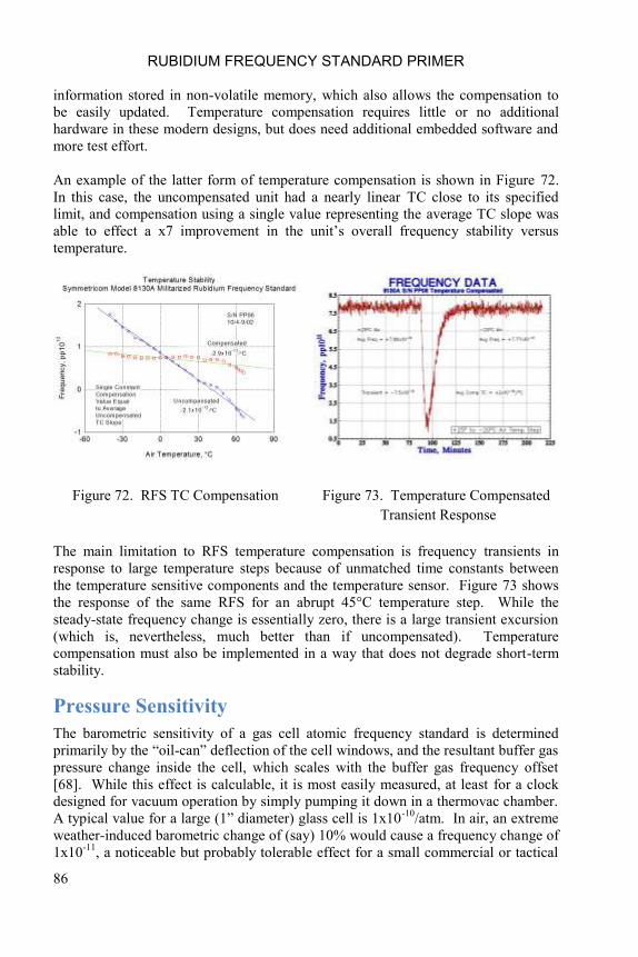
RUBIDIUM FREQUENCY STANDARD PRIMER
86
information stored in non-volatile memory, which also allows the compensation to
be easily updated. Temperature compensation requires little or no additional
hardware in these modern designs, but does need additional embedded software and
more test effort.
An example of the latter form of temperature compensation is shown in Figure 72.
In this case, the uncompensated unit had a nearly linear TC close to its specified
limit, and compensation using a single value representing the average TC slope was
able to effect a x7 improvement in the unit‟s overall frequency stability versus
temperature.
Figure 72. RFS TC Compensation
Figure 73. Temperature Compensated
Transient Response
The main limitation to RFS temperature compensation is frequency transients in
response to large temperature steps because of unmatched time constants between
the temperature sensitive components and the temperature sensor. Figure 73 shows
the response of the same RFS for an abrupt 45°C temperature step. While the
steady-state frequency change is essentially zero, there is a large transient excursion
(which is, nevertheless, much better than if uncompensated). Temperature
compensation must also be implemented in a way that does not degrade short-term
stability.
Pressure Sensitivity
The barometric sensitivity of a gas cell atomic frequency standard is determined
primarily by the “oil-can” deflection of the cell windows, and the resultant buffer gas
pressure change inside the cell, which scales with the buffer gas frequency offset
[68]. While this effect is calculable, it is most easily measured, at least for a clock
designed for vacuum operation by simply pumping it down in a thermovac chamber.
A typical value for a large (1” diameter) glass cell is 1x10⁻¹⁰
/atm. In air, an extreme
weather-induced barometric change of (say) 10% would cause a frequency change of
1x10-11
, a noticeable but probably tolerable effect for a small commercial or tactical
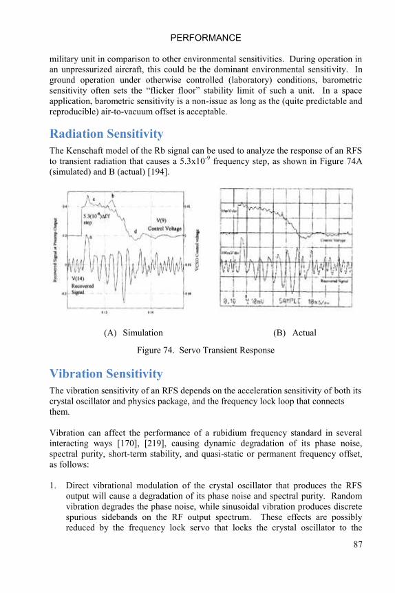
PERFORMANCE
87
military unit in comparison to other environmental sensitivities. During operation in
an unpressurized aircraft, this could be the dominant environmental sensitivity. In
ground operation under otherwise controlled (laboratory) conditions, barometric
sensitivity often sets the “flicker floor” stability limit of such a unit. In a space
application, barometric sensitivity is a non-issue as long as the (quite predictable and
reproducible) air-to-vacuum offset is acceptable.
Radiation Sensitivity
The Kenschaft model of the Rb signal can be used to analyze the response of an RFS
to transient radiation that causes a 5.3x10⁻⁹
frequency step, as shown in Figure 74A
(simulated) and B (actual) [194].
(A) Simulation (B) Actual
Figure 74. Servo Transient Response
Vibration Sensitivity
The vibration sensitivity of an RFS depends on the acceleration sensitivity of both its
crystal oscillator and physics package, and the frequency lock loop that connects
them.
Vibration can affect the performance of a rubidium frequency standard in several
interacting ways [170], [219], causing dynamic degradation of its phase noise,
spectral purity, short-term stability, and quasi-static or permanent frequency offset,
as follows:
1. Direct vibrational modulation of the crystal oscillator that produces the RFS
output will cause a degradation of its phase noise and spectral purity. Random
vibration degrades the phase noise, while sinusoidal vibration produces discrete
spurious sidebands on the RF output spectrum. These effects are possibly
reduced by the frequency lock servo that locks the crystal oscillator to the

RUBIDIUM FREQUENCY STANDARD PRIMER
88
rubidium reference. Very high vibration levels can damage a quartz crystal
resonator.
2. Crystal oscillator vibrational modulation also affects the microwave
interrogation signal applied to the rubidium physics package. Random vibration
causes noise on the Rb discriminator signal, sinusoidal vibration can cause a
quasi-static frequency offset when its frequency is related to the servo
modulation rate, and high levels of low frequency sinusoidal vibration can
reduce the applied microwave interrogation power. Sinusoidal modulation of
the microwave interrogation signal is particularly important when the vibration
frequency is twice the servo modulation rate.
3. Vibration can also affect the Rb physics package itself, mainly due to
modulation of its light throughput. Random vibration increases the noise on the
discriminator signal, while sinusoidal vibration can cause a quasi-static
frequency offset when its frequency is related to the servo modulation rate. The
latter is particularly important when the vibration frequency is equal to the servo
modulation rate. High levels of vibration can cause temporary frequency offsets
due to rubidium redistribution in the Rb spectral lamp. Very high vibration
levels can also induce mechanical damage to the physics package that can cause
permanent frequency offsets and loss of discriminator signal.
Let us first consider Item 1, the direct vibrational modulation of the crystal oscillator
that produces the RAFS output signal. The main effect of sinusoidal vibration is to
cause spurious components at a sideband frequency equal to the vibration frequency
on each side of the RF output spectrum because of the acceleration sensitivity of the
quartz crystal oscillator. The level of the discrete spectral components is determined
by the standard formula for sinusoidal FM modulation:
Sideband Level (dBc) = 20 log10 (f / 2fmod)
where f is the peak frequency deviation in Hz and fmod is the modulation rate and
sideband frequency.
For vibration, this formula for discrete FM is modified to use the peak f = g fo,
where g is the peak applied g level, is the acceleration sensitivity of the device
(expressed as a fractional frequency per g), and fo is the nominal carrier frequency:
Sideband Level (dBc) = 20 log10 (g fo / 2fvib)
Note that both the applied vibration and the vibration sensitivity are directional, and
thus a detailed analysis of the crystal resonator‟s orientation with respect to the
vibration may be required. A typical quartz crystal resonator has an acceleration
sensitivity of 1x10⁻⁹
per g along its most sensitive axis. Lower quartz crystal
resonator acceleration sensitivity is possible, either by specification or screening, and

PERFORMANCE
89
5x10⁻¹⁰
/g is feasible, but a further reduction requires special compensation
techniques.
While degrading the spectral purity, such crystal oscillator vibrational modulation
does not cause a static or permanent frequency offset. Unless the vibration level is
very high, the nominal resonant frequency of the quartz crystal is not changed, and,
even if it were, the Rb frequency lock loop would correct it. The vibrational
modulation will not affect the average RFS output frequency, and therefore will not
affect its long term time error. Low frequency vibrational disturbance of the crystal
oscillator can be corrected by the frequency lock loop to the extent that it has open
loop gain at the vibration frequency.
Next, let us consider Item 2, the effect of crystal oscillator vibrational modulation on
the microwave interrogation signal applied to the Rb physics package. Firstly, we
can usually rule out a gross loss of carrier power because the vibration would have to
be extremely large to cause a Bessel null.
But, if the vibration frequency is exactly equal to an even multiple of the RFS servo
modulation rate, there exists an intermodulation mechanism that causes the lock
point of the synchronously-detected frequency lock servo to be offset [189]. More
probably, if the (incoherent) vibration frequency is near one of those multiples of the
servo modulation rate, there will be “beats” that cause a low frequency disturbance
of the locked frequency. This instability mechanism can be quite significant. A
rough estimate for it can be based on its analogy with even-order modulation
distortion, which leads to a frequency offset value of about 1x10⁻⁹
for a -30 dBc
coherent 2fmod component. The effect can be very large, especially at the worse-case
vibration level, orientation and crystal g sensitivity for vibration at exactly twice the
modulation rate and coherent with it at a particular phasing, and it is possible for the
RFS to actually lose lock. Otherwise, one would expect degraded short-term
stability at the “beat” frequency, which would not appreciably affect the average
frequency or long term time error.
Finally, consider Item 3, the effect of vibration on the Rb physics package itself.
The moderate vibration levels under consideration are well below those imposed
during qualification testing, so it is reasonable to rule out gross effects such as
permanent damage or even Rb lamp disturbance. The main consideration is
therefore interference on the discriminator signal due to vibrational modulation of
the light beam. This depends critically on the mechanical design of the physics
package, particularly the ruggedness of the mounting of the Rb lamp, the three
ovens, and the various cells and optical elements.
EMI
RFS electronics are subject to several specific EMI considerations that are described
in the following sections of this primer.

RUBIDIUM FREQUENCY STANDARD PRIMER
90
Conducted Susceptibility
An RFS has particular susceptibility to audio frequency ripple on its DC power
supply at the servo modulation frequency and its second harmonic. For example,
ripple at the fundamental modulation rate can disturb the RFS output frequency (a)
by reaching the lamp exciter and impressing interference onto the light, (b) by
appearing at the input of the servo amplifier, (c) or by affecting the amplitude of the
RF interrogation signal, while ripple at the second harmonic of the servo modulation
rate can disturb the RFS output frequency impressing PM on the RF interrogation
signal. Such interference causes a false discriminator error signal that affects the
frequency lock servo, especially if the interference is coherent or nearly coherent
with the servo modulation. This susceptibility is difficult to completely eliminate.
Conducted Emissions
Conducted emissions from the power input of an RFS are usually associated with a
switching power supply, while must utilize an effective ripple filter to avoid this
problem. Conducted RF emission at the lamp exciter frequency is another potential
issue.
Radiated Susceptibility A properly packaged RFS should not have susceptibility problems from RF
radiation.
Radiated Emissions The most common radiated emission from an RFS is RF energy from its lamp
exciter, but proper packaging should avoid this problem.
DC Power Interface Several additional factors can impact an RFS DC power interface, including (a)
reverse polarity protection, (b) over and under voltage protection, (c) voltage
transient vulnerability, (d) input ripple current limits and (e) dynamic input
impedance, and (e) ground isolation requirements. These requirements are
particularly severe for vehicular power systems. Reverse polarity protection can be
provided by a series input diode at the expense of some inefficiency; a polarity-
sensitive relay is another possibility. Otherwise, it is wise to provide a fuse or other
sacrificial circuit element along with a shunt diode. Over voltage protection can be
provided in a similar way with a zener diode. Under voltage protection is
particularly important with a switching power supply. Protection against voltage
transients is often provided by a transient protective zener or varistor. It is
sometimes necessary to avoid high ripple currents at the series resonant frequency of
an input choke and filter capacitor, perhaps by allowing the choke to saturate and
thereby reduce the circuit Q. An assessment of the dynamic input impedance may be
necessary when the unit is powered by a switching power supply. DC ground
isolation of the input power return is usually provided by an internal DC/DC
converter, along with a balun transformer for better AC isolation.
PERFORMANCE
91
Aging
RFS frequency aging is defined as a slow change in average frequency due to effects
within the device (as compared with frequency drift which includes external
environmental effects). There is a fairly long list of possible contributors to RFS
aging, and, the better the design, the fewer of them are significant. The following
factors are generally the most important:
1. Absorption cell buffer gas (partial pressure change)
2. Light intensity and spectrum (light shift)
3. Microwave power (RF power shift)
4. C-field (voltage reference)
5. Oven temperatures (lamp and cell TCs, thermistor instability)
6. Servo offset (static and dynamic)
7. Modulation distortion (even order)
8. Microwave spectral purity (spurs, CG pulling)
For most RFS units, the first two items are the dominant causes. The best such units
show small, smooth, monotonically-stabilizing, highly-modelable and predictable
aging where, at least after initial stabilization, the direction of the aging never
reverses. Non-monotonic aging is an indication that there is more than one
significant factor, and which makes modeling difficult.
Item (1), absorption cell buffer gas pressure, has very large leverage (the total buffer
gas frequency offset which may be on the order of 1 ppm) and is subject to several
aging mechanisms, including He permeation and physical and/or chemical reaction
of the commonly-used N2 with the cell envelope or Rb film. These effects are
smooth, steady and consistent, and tend to slowly diminish with time. It is therefore
the leading candidate for the cause of RFS drift. Loss of N2 buffer gas by diffusion
into the Rb film or by weak Rb-N2 chemical reactions would cause negative aging,
as is consistently observed for the lowest-aging GPS Rb clocks. The diffusion
hypothesis is strengthened by the tendency of the aging of those units to be well-
modeled as proportional to the square root of time.
Item (2), light shift, is a popular aging mechanism invoked because it can also have
significant leverage and it is likely that the lamp output will change over time. It is
undoubtedly a significant factor in the aging of most RFS, but probably not for the
lowest-aging GPS Rb clocks that are carefully adjusted for a zero light shift (ZLS)
condition by adjusting the temperature of their discrete filter cell
Item (3), microwave interrogation power, depends on the RF power sensitivity of the
particular design, which is much larger for units employing an integrated resonance
cell than those with separate filter and absorption cells. The lowest-aging GPS Rb
clocks have an RF sensitivity of about ±2x10-12
/dB and highly-stabilized RF
interrogation power, and their aging is not believed to be affected by this factor.
Clearly there cannot be a large long-term RF power change because of the resulting

RUBIDIUM FREQUENCY STANDARD PRIMER
92
unobserved effect that would have on the magnitude of the recovered 2nd harmonic
signal. For example, a 1 dB change per year, more than would be inferred from the
signal record, corresponds to an aging contribution of only 5x10-15
/day.
Item (4), C-field, is an obvious but insignificant factor. One can estimate and
exclude instability of the zener diode that controls the C-field. A 10 ppm/month
voltage stability corresponds to an aging of only about 1x10-15
/day for a unit
operating at a low (50 mG) C-field.
Item (5), oven temperature change, is also very small. The thermistors that control
the oven temperatures have ±0.05%/year stability, and, for the filter cell oven with
the largest -6x10-11
/ºC TC, this would cause an aging of under 3x10-15
/day.
Items (6)-(8), electronic effects like servo offsets, modulation distortion and
microwave spurs can be analyzed and shown to be OK.
Some more details about aging mechanisms in a rubidium gas cell frequency
standard are as follows:
1. Permeation of helium through the walls of the absorption cell is a well-
understood reason for negative RFS aging in vacuum. Helium has a high
positive pressure shift coefficient (PC), +720 Hz/Torr. During storage in air, it
can enter the cell by permeation through the glass envelope, thereby raising the
frequency. Then, during subsequent operation in vacuum, the He would leak
out, causing negative frequency aging with a long stabilization time. A glass
type having low helium permeation (e.g., Corning 7056) should be used for the
absorption cell envelope.
2. Loss of N2 buffer gas partial pressure in the absorption cell is another potential
drift mechanism. The PC of N2 is +548 Hz/Torr, and change in its partial
pressure of only -1.25x10⁻⁶
Torr/day would cause a cell using that common
buffer gas to drift -1x10-13
/day.
Permeation is not a plausible mechanism for N2 loss. Gross leaks are unlikely,
and would show obvious signs of Rb oxidation while in air. But interaction
between nitrogen and the rubidium film in the absorption cell is a possible way
that N2 could be lost. Such interactions could be chemical reactions or (more
likely) physical adsorption. It is well known that large negative aging (pp1010
)
takes place immediately after an absorption cell containing a pure or partial N2
buffer gas is made, and that the aging of a cell is affected by disturbing the thin
Rb film that forms on its inside walls. This film, although invisible, is
electrically conductive, as indicated by the increase in the microwave loss of a
cavity into which a freshly-chased cell is placed. A monolayer of N2 on the
absorption cell wall represents a frequency offset of 7x10⁻⁹
, so an aging of
1x10-13
corresponds to a change of only about 14 ppm of a monolayer. The long
aging time constant is consistent with slow Rb redistribution, which requires
PERFORMANCE
93
about 200 days to move the length of the absorption cell under the influence of a
0.1C temperature gradient.
3. Much the same argument can be applied to N2-glass reactions. A very small rate
of N2 partial pressure reduction due to reaction with the absorption cell glass
envelope could account for gradually decreasing negative frequency aging
4. Hydrocarbon contamination, perhaps as a buffer gas trace constituent, could be a
concern because it would likely have a very large pressure shift coefficient (e.g.
heptane (C7H16) has a PC ≈ -4.5 kHz/Torr).
5. Changes in the intensity and spectrum of the Rb lamp used as the optical
pumping light source, because of changes in the lamp exciter RF power, lamp
oven temperature, lamp Rb distribution, lamp mounting thermal conductivity,
light beam darkening, etc., can cause frequency changes due to the light shift
effect. A classical RFS uses a “double-resonance” technique whereby the
optical pumping (state selection) and microwave interrogation are performed
simultaneously. This causes the frequency to depend on the optical pumping
conditions, causing a so-called light shift coefficient (LSC). Most RFS operate
at a condition of nominal zero. It is likely that a significant portion of the RFS
flicker FM noise floor is determined by lamp intensity and spectral fluctuations
via residual light shift effects, but there is no compelling reason to believe that
lamp changes and residual LSC is the dominant cause of long-term RAFS drift,
especially if it is always in the same direction.
6. Frequency drift could be caused by changes in the DC magnetic bias field
caused by (a) drift of the reference zener and other electronic components
associated with the C-field source, or (b) changes in the cavity oven residual
heater field caused by changes in the thermal losses or external temperature
producing a change in the heater power, or (c) changes in internal residual
magnetism, or (d) changes in the external magnetic field environment
7. A change in the temperatures of the lamp, filter cell and cavity ovens because of
aging of their control thermistors would cause frequency drift due to the
temperature sensitivity of the Rb lamp, filter cell and absorption cell. Such an
effect could cause frequency aging that would slowly stabilize with time.
8. A change in cavity RF magnetic field strength because of change in the RF drive
level, the step-recovery diode multiplier conversion gain or the microwave
cavity Q would cause frequency drift due to RF power sensitivity. An SRD
multiplier output can change because of component variations and bias circuit
changes. The cavity Q (which determines the relationship between the RF
power and magnetic field strength) can vary because of Rb migration within the
absorption cell. RFS RF power sensitivity is caused primarily by spatial
inhomogeneity due to DC and RF magnetic field variations and temperature
gradients within the absorption cell that cause the frequency to vary within the
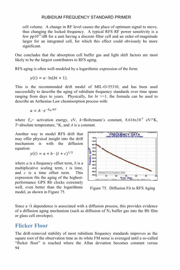
RUBIDIUM FREQUENCY STANDARD PRIMER
94
cell volume. A change in RF level causes the place of optimum signal to move,
thus changing the locked frequency. A typical RFS RF power sensitivity is a
few pp1012
/dB for a unit having a discrete filter cell and an order-of-magnitude
larger for an integrated cell, for which this effect could obviously be more
significant.
One concludes that the absorption cell buffer gas and light shift factors are most
likely to be the largest contributors to RFS aging.
RFS aging is often well-modeled by a logarithmic expression of the form:
( ) ( )
This is the recommended drift model of MIL-O-55310, and has been used
successfully to describe the aging of rubidium frequency standards over time spans
ranging from days to years. Physically, for bt >>1, the formula can be used to
describe an Arrhenius Law chemisorption process with:
⁄
where Ea= activation energy, eV, k=Boltzmann‟s constant, 8.616x10⁻⁵
eV/K,
T=absolute temperature, K, and A is a constant.
Another way to model RFS drift that
may offer physical insight into the drift
mechanism is with the diffusion
equation:
( ) ( ) ⁄
where a is a frequency offset term, b is a
multiplicative scaling term, t is time,
and c is a time offset term. This
expression fits the aging of the highest-
performance GPS Rb clocks extremely
well, even better than the logarithmic
model, as shown in Figure 75.
Figure 75. Diffusion Fit to RFS Aging
Since a t dependence is associated with a diffusion process, this provides evidence
of a diffusion aging mechanism (such as diffusion of N2 buffer gas into the Rb film
or glass cell envelope).
Flicker Floor
The drift-removed stability of most rubidium frequency standards improves as the
square root of the observation time as its white FM noise is averaged until a so-called
“flicker floor” is reached where the Allan deviation becomes constant versus
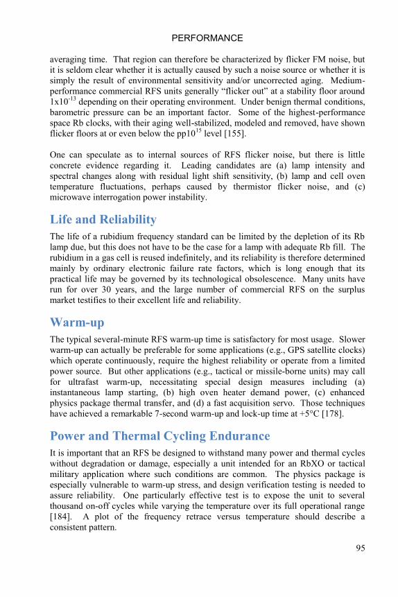
PERFORMANCE
95
averaging time. That region can therefore be characterized by flicker FM noise, but
it is seldom clear whether it is actually caused by such a noise source or whether it is
simply the result of environmental sensitivity and/or uncorrected aging. Medium-
performance commercial RFS units generally “flicker out” at a stability floor around
1x10-13
depending on their operating environment. Under benign thermal conditions,
barometric pressure can be an important factor. Some of the highest-performance
space Rb clocks, with their aging well-stabilized, modeled and removed, have shown
flicker floors at or even below the pp1015
level [155].
One can speculate as to internal sources of RFS flicker noise, but there is little
concrete evidence regarding it. Leading candidates are (a) lamp intensity and
spectral changes along with residual light shift sensitivity, (b) lamp and cell oven
temperature fluctuations, perhaps caused by thermistor flicker noise, and (c)
microwave interrogation power instability.
Life and Reliability
The life of a rubidium frequency standard can be limited by the depletion of its Rb
lamp due, but this does not have to be the case for a lamp with adequate Rb fill. The
rubidium in a gas cell is reused indefinitely, and its reliability is therefore determined
mainly by ordinary electronic failure rate factors, which is long enough that its
practical life may be governed by its technological obsolescence. Many units have
run for over 30 years, and the large number of commercial RFS on the surplus
market testifies to their excellent life and reliability.
Warm-up
The typical several-minute RFS warm-up time is satisfactory for most usage. Slower
warm-up can actually be preferable for some applications (e.g., GPS satellite clocks)
which operate continuously, require the highest reliability or operate from a limited
power source. But other applications (e.g., tactical or missile-borne units) may call
for ultrafast warm-up, necessitating special design measures including (a)
instantaneous lamp starting, (b) high oven heater demand power, (c) enhanced
physics package thermal transfer, and (d) a fast acquisition servo. Those techniques
have achieved a remarkable 7-second warm-up and lock-up time at +5°C [178].
Power and Thermal Cycling Endurance
It is important that an RFS be designed to withstand many power and thermal cycles
without degradation or damage, especially a unit intended for an RbXO or tactical
military application where such conditions are common. The physics package is
especially vulnerable to warm-up stress, and design verification testing is needed to
assure reliability. One particularly effective test is to expose the unit to several
thousand on-off cycles while varying the temperature over its full operational range
[184]. A plot of the frequency retrace versus temperature should describe a
consistent pattern.

RUBIDIUM FREQUENCY STANDARD PRIMER
96
Storage
Long-term off storage is not a severe problem for RFS units, but there are several
considerations that are worth keeping in mind. An RFS should be stored at room
temperature and away from a source of helium. One generally assumes that the
failure rate during storage is less (say one-half) of that during normal operation
because there are no electrical stresses applied and internal temperatures are lower.
Periodic Turn-On
It is not necessary to periodically turn on an RFS during prolonged storage.
Nevertheless, for critical applications, it is probably desirable to do so (say for 24
hours at 6-month intervals) to allow the physics package to re-stabilize.
Lamp Starting After Prolonged Storage
One concern regarding prolonged RFS storage is the possible failure of the Rb lamp
to start. This concern is primarily associated with slow migration of excess rubidium
from the tip of the lamp into the active region where the discharge is excited. The
resulting Rb film on the inside surface of the glass lamp envelope could then load the
lamp exciter circuit to such an extent that it would not oscillate, and the lamp would
never start.
Excess rubidium (more than that needed to support a saturated vapor pressure at the
operating temperature) is necessary to assure sufficient lamp life. This excess
rubidium (about 100 µgrams, liquid at temperatures above 39°C) collects in the tip
(cold spot) of the lamp during normal operation. When the RFS is off, the rubidium
is “frozen” and nearly all of it remains in the tip. Nevertheless, it still has a finite
vapor pressure, and under the influence of any temperature gradient, could migrate to
another locating within the lamp. This is a very slow process, especially at relatively
cool temperatures with the whole lamp at the same temperature, but, over a long
period of time, can result in some rubidium condensed in the active region of the
lamp.
The Rb lamp exciter is an RF power oscillator delivering about 0.5 watt at about 115
MHz to the lamp located inside its tank coil. The unlit lamp normally presents a
very light load to the exciter, which then has excess loop gain and easily starts
oscillating. The high RF voltage associated with the lightly-loaded tank circuit along
with some initially-ionized buffer gas atoms lights a plasma discharge in the lamp.
As the lamp oven heats, the Rb vapor pressure rises, and the lower ionization
potential of Rb causes the lamp discharge to emit light at the two Rb “D” lines that
provide optical pumping for the RFS.
The most essential aspect of this lamp starting process is that the RF exciter has
sufficient loop gain to oscillate. If it does, even if loaded by condensed rubidium,
the resulting RF induction heating will cause the rubidium to rapidly migrate away
from the discharge region to the cooler lamp tip, the tank Q and RF voltage will

PERFORMANCE
97
increase, and the lamp will start. A successful lamp exciter design must recognize
and overcome those issues by having sufficient RF exciter power, perhaps boosting it
for lamp starting. It is relatively easy to provide adequate margin, and the failure of
even a heavily-loaded lamp exciter circuit to oscillate is very unusual, thus assuring
that the lamp will start after prolonged storage.
Helium Permeation into the Absorption Cell
Helium gas in the atmosphere can permeate through the walls of the glass absorption
cell and thereby affect its buffer gas and frequency. For a unit stored and operated in
air, this is not an important issue unless the unit is stored in a location with an
atmosphere enhanced in helium. It will eventually each equilibrium with the
atmospheric helium tension and the helium diffusion rate is lower when the cell is
cool during off storage. But for a space Rb clock, the helium will diffuse out again
in vacuum, so, if it has “breathed in” helium during ground storage the unit will
show negative frequency aging as the helium diffuses out [126]. In that application,
it is recommended that the unit be stored in a helium-free (e.g., dry nitrogen)
atmosphere.
Applications
RFS applications can be divided into commercial, military and space sectors.
Commercial RFS units are distinguished primarily by their low cost, made feasible
mainly by the economies of scale created by telecom usage. Those applications have
also driven size reductions and extended their upper operating temperature range,
with less emphasis on best stability and performance. Nevertheless, commercial
RFS units have gotten smaller and cheaper with only modest reductions in
performance, a result fundamentally enabled by the remarkable ability to achieve
strong, narrow resonance line in a small gas cell utilizing buffer gas.
Military RFS units are distinguished by their ability to perform reliably from
unconditioned power in harsh environments such as shock, acceleration and
vibration, extreme temperatures, and exposure to moisture, humidity, EMI and
radiation. In the past, such units were often developed specifically to satisfy the
need of a particular program according to standard military specifications and
employing special MIL-spec parts. Today, the RFS units used in most military
equipment are based on ruggedized versions of commercial-off-the shelf (COTS)
designs. That results in significant cost savings and faster development schedules,
and is feasible in large part because of the improved reliability of commercial
electronic parts. It is still necessary, however, to consider the demands of the
military environment and to modify and qualify a commercial RFS design as
necessary to satisfy those demands.
Phase noise and spectral purity under vibration is often a concern for a MIL RFS,
and may require that the crystal oscillator and physics package be modified
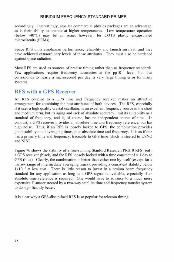
RUBIDIUM FREQUENCY STANDARD PRIMER
98
accordingly. Interestingly, smaller commercial physics packages are an advantage,
as is their ability to operate at higher temperatures. Low temperature operation
(below -40°C) may be an issue, however, for COTS plastic encapsulated
microcircuits (PEMs).
Space RFS units emphasize performance, reliability and launch survival, and they
have achieved extraordinary levels of those attributes. They must also be hardened
against space radiation.
Most RFS are used as sources of precise timing rather than as frequency standards.
Few applications require frequency accuracies at the pp1011
level, but that
corresponds to nearly a microsecond per day, a very large timing error for many
systems.
RFS with a GPS Receiver
An RFS coupled to a GPS time and frequency receiver makes an attractive
arrangement for combining the best attributes of both devices. The RFS, especially
if it uses a high quality crystal oscillator, is an excellent frequency source in the short
and medium term, but its aging and lack of absolute accuracy limit its suitability as a
standard of frequency, and it, of course, has no independent source of time. In
contrast, a GPS receiver provides an absolute time and frequency reference, but has
high noise. Thus, if an RFS is loosely locked to GPS, the combination provides
good stability at all averaging times, plus absolute time and frequency. It is as if one
has a primary time and frequency, traceable to GPS time which is steered to USNO
and NIST.
Figure 76 shows the stability of a free-running Stanford Research PRS10 RFS (red),
a GPS receiver (black) and the RFS loosely locked with a time constant of ≈ 1 day to
GPS (blue). Clearly, the combination is better than either one by itself (except for a
narrow range of intermediate averaging times), providing a consistent stability below
1x10-11
at low cost. There is little reason to invest in a cesium beam frequency
standard for any application as long as a GPS signal is available, especially if an
absolute time reference is required. One would have to advance to a much more
expensive H-maser steered by a two-way satellite time and frequency transfer system
to do significantly better.
It is clear why a GPS-disciplined RFS is so popular for telecom timing.
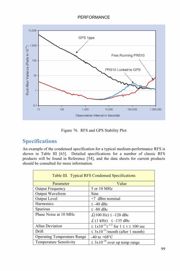
PERFORMANCE
99
Figure 76. RFS and GPS Stability Plot
Specifications
An example of the condensed specification for a typical medium-performance RFS is
shown in Table III [63]. Detailed specifications for a number of classic RFS
products will be found in Reference [54], and the data sheets for current products
should be consulted for more information.
Table III. Typical RFS Condensed Specifications
Parameter Value
Output Frequency 5 or 10 MHz
Output Waveform Sine
Output Level +7 dBm nominal
Harmonics -40 dBc
Spurious -80 dBc
Phase Noise at 10 MHz L(100 Hz) -120 dBc
L (1 kHz) -135 dBc
Allan Deviation 1x10-11
-1/2 for 1 100 sec
Drift 3x10-11
/month (after 1 month)
Operating Temperature Range -40 to +68C
Temperature Sensitivity 3x10⁻¹⁰
over op temp range

RUBIDIUM FREQUENCY STANDARD PRIMER
100
Parameter Value
Supply Voltage +22 to +32 VDC
Power 30 W (max), 12 W (SS, +25C)
Warm-up Time 5 min to lock at +25C
Voltage Sensitivity 1x10-11
/10%
Magnetic Field Sensitivity 2x10-11
/Gauss
Size (L, W, H) 3” x 3” x 4”
Testing
Environmental performance is critical for many applications of rubidium frequency
standards. IEEE Standard 1193, IEEE Guide for Measurement of Environmental
Sensitivities of Standard Frequency Generators [256] and Section 4.9 of MIL-O-
55310B for crystal oscillators [253] provide guidelines for the testing of these
devices, but a custom test plan and procedure is often required.
Rubidium frequency standards are, for the most part, tested similarly to other pieces
of electronic equipment. Commercial RFS units are subject to their manufacturer‟s
normal development tests, followed by those production tests deemed necessary to
maintain product quality, while military and space clocks are subject to more
stringent developmental, qualification and acceptance testing as dictated by program
requirements and their specifications.
The main differences associated with RFS tests are (a) the need for an adequate
frequency reference and specialized clock measuring facilities, and (b) the need to
verify RFS long-term aging which requires that units be operated for an extended
period of time. Space RFS testing imposes the additional requirement of conducting
the tests under thermovac conditions. RFS testing is described comprehensively in
Reference [69] in the context of military specification requirements.
Table IV. Military Specifications for the Testing of Electronic Equipment
RFS
USAGE
GENERAL
SPECIFICATION
TEST
REQUIREMENTS
ENVIRONMENTAL
TEST METHODS
EMI TEST
METHODS
A11 MIL-STD-454 MIL-STD-810 MIL-STD-461
Airborne MIL-E-5400 MIL-T-5422
Ship MIL-E-16400
Ground MIL-E-4158
Space DOD-E-8983 MIL-STD-1540 MIL-STD-1541
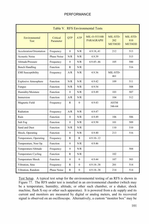
PERFORMANCE
101
Table V. RFS Environmental Tests
Environmental
Test
Critical
Parameter
QTP ATP MIL-O-55310B
PARAGRAPH
MIL-STD-
202
METHOD
MIL-STD-
810
METHOD
Acceleration/Orientation Frequency 0 N/R 4.9.18,.41 212 513
Acoustic Noise Phase Noise N/R N/R 4.9.39 515
Altitude/Pressure Frequency 0 N/R 4.9.45-.46 105 500
Bench Handling Function R N/R 516
EMI Susceptibility Frequency A/R N/R 4.9.36 MIL-STD-
461
Explosive Atmosphere Function N/R N/R 4.9.42 109 511
Fungus Function N/R N/R 4.9.54 508
Humidity/Moisture Function 0 N/R 4.9.49 103 507
Immersion Function A/R N/R 104 512
Magnetic Field Frequency R 0 4.9.43 ASTM
346-64
Radiation Frequency A/R N/R 4.9.47
Rain Function 0 N/R 4.9.49 106 506
Salt Fog Function 0 N/R 4.9.50 101 509
Sand and Dust Function N/R N/R 110 510
Shock, Operating Function 0 N/R 4.9.40 213 516
Temperature, Operating Frequency R R 4.9.10-.12
Temperature, Non Op. Function 0 N/R 4.9.46
Temperature/Altitude Frequency 0 N/R 504
Temperature Cycling Function R N/R 102
Temperature Shock Function 0 0 4.9.44 107 503
Vibration, Sine Frequency R 0 4.9.18-.38 201 514
Vibration, Random Phase Noise R 0 4.9.18-.38 214 514
Test Setup. A typical test setup for the environmental testing of an RFS is shown in
Figure 77. The RFS under test is installed in an environmental chamber (which may
be a temperature, humidity, altitude, or other such chamber, or a shaker, shock
machine, flash X-ray or other such apparatus). It is powered from a dc supply and its
current and monitors are measured by digital or analog meters, and its recovered
signal is observed on an oscilloscope. Alternatively, a custom “monitor box” may be

RUBIDIUM FREQUENCY STANDARD PRIMER
102
used, especially if special control or monitor functions are involved. A stripchart
record of the RFS dc supply current is often useful for evaluating performance and
diagnosing problems. Besides warm-up and steady-state power, the current record
shows lamp ignition and oven stability, and can be integrated to determine RbXO
syntonization energy [184]. The primary measurements, however, are the RFS RF
output level, frequency, and spectral purity. The frequency measuring system may
be simply a vector voltmeter or analog frequency difference meter to measure RFS
phase or frequency change, a frequency counter (perhaps the high resolution
interpolating reciprocal type), or a very high resolution heterodyne arrangement
(perhaps with computer control and data analysis). The frequency reference may be
a crystal oscillator (for low noise), another rubidium standard (for stability,
portability, and fast warm-up), or a cesium standard (for absolute frequency
determination). The RFS spectral purity may be observed on an RF spectrum
analyzer or on a wave or FFT analyzer (after down conversion). A phase noise
measuring system may also be necessary (by using a double-balanced mixer and
loose phase-locked crystal oscillator). The primary concern for this instrumentation
is often its portability to an outside testing lab. In such a case, careful planning is
critical and all the test instrumentation should be set up “at home” to confirm the test
methodology and to avoid missing or malfunctioning items in the field.
Figure 77. RFS Environmental Test Setup
Acceleration/Orientation. Unlike a quartz crystal oscillator, an RFS does not have
any inherent static acceleration sensitivity (either “tip-over effect” or centrifuge). It
is possible, however, for an RFS to show some frequency change due to acceleration
and reorientation because of thermal effects. A test for RFS orientation sensitivity
should therefore allow sufficient time (about five minutes) to reestablish thermal
equilibrium. It is also possible to have some change in the physical distribution of
the rubidium in the lamp under high static g-forces that can cause a small frequency

PERFORMANCE
103
change. This effect will occur if the acceleration forces liquid rubidium into the
body of the lamp and will be reversed by acceleration in the opposite direction or by
quiescent operation. It is possible, but not always easy, to make the precision
frequency measurements necessary to see these effects via the slip rings of a
centrifuge. Redundant slip rings should be used for both power and RFS output to
reduce contract noise.
A separate “2g tip-over” test may be required for the crystal oscillator portion of an
RbXO. The test results should be reported as the resultant of the g-sensitivity vector.
Dynamic acceleration can have a profound effect on the stability and purity of an
RFS, and those tests are discussed in the Vibration section below.
Acoustic Noise. Acoustic noise is usually not a significant factor affecting RFS
operation. The RFS is typically suspended on elastic cords during exposure;
frequency and phase noise should be measured.
Altitude/Barometric Pressure. The main considerations for the sensitivity of an RFS
to ambient pressure are; (a) frequency shift due to absorption cell buffer gas pressure
change caused by deflection of the glass cell envelope (about 1x10⁻¹⁰/atm), (b)
frequency shift due to thermal effects involving the physics package ovens and Rb
lamp, and (c) thermal effects due to heat transfer of the electronic circuits. Effect (a)
is proportional to the pressure change; effects (b) and (c) are small until the pressure
is reduced to about 10 Torr (100,000 feet altitude). Oven power will be less and
stabilization factor better in vacuum. The electronic circuits must be designed for
adequate heat transfer without air, and temperature profiling may be necessary to
ensure reliable operation in vacuum. The barometric sensitivity of an RFS can also
be measured as part of a temperature-altitude test. Unlike a cesium beam frequency
standard, an RFS does not use high voltages and can be safely operated throughout
the full pressure range from sea level to hard vacuum without any corona discharge
hazard.
Bench Handling. A bench handling shock test is perhaps the most severe yet
realistic and practical way to check an RFS for ruggedness. The unit should be
removed from its enclosure as it if were being serviced. After completing the test,
the unit should be inspected for damage and operated to show any resulting
frequency offset.
EMI Susceptibility. The most significant form of EMI susceptibility in an RFS is
usually due to ripple (CS01) and transients (CS06) on the dc input power. This
aspect of RFS design is covered by military and other standards [257], but specific
requirements may also be imposed. Ripple susceptibility is generally worst at the
RFS servo modulation rate; large frequency offsets are possible due to interference
with the servo that locks the VCXO to the Rb reference. A phase comparator, vector
voltmeter, or analog frequency difference meter is very useful for showing RFS EMI
susceptibility, as is observation of the RFS recovered signal on an oscilloscope.
Ripple susceptibility testing does not require a screen room or specialized EMI test

RUBIDIUM FREQUENCY STANDARD PRIMER
104
instrumentation, and can be investigated with ordinary laboratory equipment. The
EMI susceptibility test procedure must include a pass/fail criterion; a frequency
change of 1x10⁻¹⁰ is a reasonable value for a tactical RFS. The radiated
susceptibility test setup should pay particular attention to the shielding and
grounding of the RFS power/monitor leads; this is often the primary path for
interfering RF into the unit. It is also advisable to use a low-noise linear (rather than
switching) dc supply to power the RFS during all EMI testing.
The requirements for transient protection vary depending on the degree of external
power conditioning. Reverse and overvoltage protection is often necessary and must
be tested. Applying a pre-charged capacitor across the dc input is one simple way to
simulate voltage transients. RFS turn-on (inrush current) and turn-off (voltage spike)
transients can be a problem for the host system. A manually tipped mercury relay
and a digital storage oscilloscope is an effective means to simulate and observe these
transients.
Explosive Atmosphere. An RFS does not use high voltages or mechanical relays and
switches, and can be operated in an explosive atmosphere with minimal likelihood of
causing an explosion. Since an RFS is not normally sealed, the outer cover should
be removed or loosened during the test to facilitate the penetration of the explosive
vapor.
Fungus. A fungus test is usually conducted “by analysis” to verify that the design
uses only components and materials that are inherently fungus inert.
Humidity/Moisture. A typical humidity test consists of five, 48-hour temperature-
humidity cycles with RFS operation near the end of each cycle. With an unsealed
unit, the test results depend strongly on the adequacy of conformal coating and
encapsulating processes, and these should closely represent the actual production
processes for the test results to be valid. RFS moisture sensitivity is most often
associated with the high impedance servo amplifier synchronous detector/integrator
circuits.
Immersion. The capability to withstand immersion in water is seldom a requirement
for an RFS. Immersibility requires a sealed case and connectors, but it otherwise
does not affect RFS design or performance.
Intermittent Operation/Retrace. (See Power/ Temperature Cycling below.) A test
for the frequency retrace of an RFS under intermittent operation should, by
definition, return the unit to exactly the same operating conditions so as not to
confuse retrace with environmental sensitivity. The main concern is that the retrace
error be non-accumulative. The test must define; (a) operating conditions
(temperature, etc.), (b) off time, (c) restabilization time, and (d) number of retrace
cycles. A well-designed RFS should have an excellent retrace characteristic
(pp1011) that has little dependency on temperature, off time, or restabilization time.

PERFORMANCE
105
The test emphasis should therefore be on performing enough cycles to verify that the
retrace error does not accumulate.
Magnetic Field. An RFS has an inherent sensitivity to dc magnetic field and con-
tains magnetic shielding to reduce this sensitivity. The largest magnetic sensitivity is
along the physics package optical axis (the direction of the internal bias field), and
has a quadratic dependence of frequency on dc magnetic field (f/f = 8.38x10⁻⁸ H,
Gauss2). Since the magnetic sensitivity varies with C-field frequency adjustment,
the test procedure must specify the RFS frequency setting (minimum, nominal, upper
range, or maximum); nominal is usually used.
The test procedure must also define the magnetic field environment. The electrical
reversal of a 3 Gauss field from a pair of 4 foot diameter Helmholtz coils [89] is
recommended. This field is easy to produce yet considerably larger than the Earth‟s
field of about 0.5 Gauss, and field reversal tends to eliminate offsets due to the
Earth‟s field (a shielded room is impractical). Other considerations for the test field
are; (a) uniformity using coils much larger than RFS and away from metallic objects,
(b) calibration (measure field at center w/o RFS), and (c) magnitude which affects
shielding factor and measurement resolution. Care should be exercised when de-
energizing the Helmholtz coils; unplugging them can produce a hazardous high
voltage.
Magnetic sensitivity is generally a qualification test, but variations in C-field and/or
shield permeability and fit can require 100% testing for critical applications. AC
magnetic field sensitivity is generally part of EMI susceptibility testing.
Radiation. The radiation sensitivity of an RFS is essentially that of its electronic
circuits; the Rb physics package is inherently quite hard. RFS survivability can be a
critical requirement for both transient and total dose radiation environments.
Transient radiation testing usually requires a Flash X-Ray (FXR) facility to generate
an intense gamma pulse. The RFS is operated during the exposure and may be
required to “operate through” or to quickly recover frequency accuracy; in all cases,
it must not suffer latch-up, burnout, or other permanent degradation. The test setup
generally includes extensive recording of RFS output level, phase, frequency, light
monitor, VCXO control voltage, and dc input current (as well as radiation
dosimetry). Transient radiation testing is very desirable to verify analysis of the RFS
circuits, and is meaningful even for a single sample having generic parts. The most
critical parts causing latch-up are usually CMOS devices; all circuits may require
resistors or other means for current limiting.
Total dose radiation testing requires a different methodology. Analysis based on
piece-part test data is often preferable to a test of the entire RFS because a worst-case
error budget can be done. The most critical devices are usually servo amplifier and
temperature controller op amps and the C-field voltage reference. RFS testing, if
done to confirm the analysis, must be done with hardened parts. Total dose testing is
likely to damage the unit as it is exposed to a series of successively higher radiation
RUBIDIUM FREQUENCY STANDARD PRIMER
106
levels. The test setup is usually quite simple if the unit does not have to be operated
during the exposure; before and after frequency and perhaps monitor measurements
are generally all that is required. Total gamma dose is usually done by placing the
unit in a Co60 cell. Dose rate and annealing effects should be considered. If the unit
is operating during exposure, the RFS photodetector will respond to the gamma
irradiation. Neutron exposure is usually done by placing the unit in a reactor. The
unit may become radioactive because of neutron activation of the magnetic shields
and other high-Z materials. The most critical part for neutron fluence is usually the
silicon photodetector, which loses output due to lattice damage.
No standard procedures apply to RFS radiation testing; each case requires careful
planning and expert advice.
Rain. The test procedure should specify which sides of the RFS are to be exposed to
rain. Typically, waterproof cables are attached throughout the test, and the unit is
operated near the end of each exposure.
Salt Fog. Since the RFS is typically not operated during exposure, its connectors
should be covered. The unit should not be washed after exposure (as allowed by
MIL-STD-810). EMI testing should follow salt fog exposure since salt deposits and
corrosion could affect grounding and shielding. This can be a very destructive test.
Sand and Dust. The test procedure should specify the RFS face to be exposed.
Since the RFS is non-operating during exposure, connectors should be covered.
Penetration of dust should not necessarily be considered a failure.
Shock. The RFS under test should be powered to best show intermittent failures
under shock. Test cables should have strain relief and should be supported close to
the unit to prevent whipping and damage which could affect RFS measurements.
The RFS should be observed for timing error and permanent frequency offset.
Rubidium motion in the lamp (as described under Acceleration) may occur.
Temperature, Operating. Temperature sensitivity is often the most significant
environmental factor affecting the performance of an RFS. A stability of 3x10⁻¹⁰ is
typical for a small tactical RFS over a military temperature range, whereas the unit
will not have that much frequency aging over several years. Furthermore, there is
considerable unit-to-unit variation of this important parameter which is not
necessarily monotonic and which may have regions of high incremental sensitivity.
The RFS temperature stability is usually specified as the maximum (peak-to-peak)
variation in frequency anywhere within the operating temperature range. RFS
operating temperature range is usually specified from a minimum ambient value to a
maximum baseplate value. The distinction between ambient and baseplate
temperatures is necessary because of the RFS internal dissipation unless the unit is
attached to a large heat sink or is otherwise well coupled to the ambient. It is
sometimes necessary to specify the thermal resistance of the heat sink (from ambient
air to RFS baseplate).
PERFORMANCE
107
RFS temperature stability should be measured as part of the ATP for every unit. It is
best to make continuous frequency measurements on a stripchart recorder as the RFS
is stepped or ramped over its full operating temperature range (rather than just
measure the RFS frequency at a few discrete temperatures) so that a region of large
sensitivity or anomalous behavior is detected. An averaging time should be chosen
long enough to average the measurement noise while not masking rapid changes;
100 seconds is usually a good choice. Sufficient dwell time must be allowed,
especially at the temperature extremes, and the record should be examined for noise,
“glitches,” and retrace.
If the RFS uses C-field temperature compensation, it may exhibit disparate
frequency-temperature characteristics at different frequency adjustments.
Temperature, Non-Operating. Sufficient soak time must be used to ensure that RFS
internal temperatures reach the specified limits.
Temperature Cycling. (See Power/Temperature Cycling below).
Temperature Shock. Temperature shock testing is not as effective with an RFS as
with small components because of the slow internal temperature response of the
ovens. The severity of the test is indicated more by the internal temperature
extremes than the rate of change of ambient temperature, which may be expensive to
produce.
Temperature/Altitude. The Temperature/Altitude test has been deleted from the
latest revision of MIL-STD-810. It is better to measure the effects of pressure
(altitude) and temperature separately.
Vibration. The stability and purity of an RFS are affected by mechanical vibration
primarily because of the acceleration sensitivity of the quartz crystal used in the
VCXO that produces the output signal. Direct vibrational modulation of the crystal
oscillator generally affects the RFS phase noise and spectral purity at vibration
frequencies higher than the servo bandwidth without producing a frequency offset.
Vibrational modulation of the VCXO at the 2nd harmonic of the servo modulation
rate, however, can cause a frequency offset. Low frequency vibrational modulation
of the crystal oscillator can cause a frequency offset due to loss of microwave power.
These XO effects are reduced by a high modulation rate, a wide servo bandwidth,
and a low crystal g-sensitivity.
RFS stability can also be affected by vibrational modulation of the physics package
light beam at or near the servo modulation rate. This problem is reduced by rigid
physics package construction. Circuit board and wiring microphonics can also affect
RFS stability.
RFS vibration testing requires measurement of frequency offset, frequency stability
(Allan deviation) and phase noise under dynamic conditions while the unit is on a
shaker. It should also include before and after measurements to check for a per-

RUBIDIUM FREQUENCY STANDARD PRIMER
108
manent frequency offset. Phase noise is the primary parameter of concern during
random vibration, and frequency stability is the most critical factor under sine
vibration. Particular attention should be paid to frequency stability while the RFS is
vibrated at the servo modulation rate and its harmonics. An analog frequency
difference meter is an effective measurement tool; counter measurements are subject
to beats due to coherence between the gate time and vibration frequency. The RFS
recovered signal should also be observed, as should the lock detector output. Checks
should be made for interference from the magnetic field of an electrodynamic shaker
by holding the unit slightly above the top of the operating shaker. A slip table can
help by allowing separation between the shaker and the RFS under test, and it also
reduces cross-axis vibration. Ground insulation (rigid) or an isolation transformer in
the RFS output can also help to avoid ground loops, hum and interference; sine dwell
measurements should not be made at 60 Hz harmonics.
Power/Temperature Cycling
RFS units intended for frequent on-off and temperature cycling (in particular, the Rb
reference of an RbXO [184]) should be subjected to a Design Verification Test
(DVT) to prove their endurance under such cycling. The physics package of a fast-
warm-up RFS turned on after a cold soak experiences severe thermal stresses;
nevertheless, with proper design, a unit can survive such cycling and provide a
stability comparable to a unit that operates continuously. A typical DVT would
subject four RFS units to 20 on-off cycles per day while subjecting them to a -62 to
+68C temperature cycle each day for 180 days. The daily temperature cycles
include a cold soak at the low temperature extreme. The internal temperature of the
Rb physics package should decay essentially all the way to the air temperature
between turn on. The 3600 on-off cycles and 180 temperature cycles of the DVT
simulate 20 years of normal RFS operation.
The DVT should also include frequency measurement data after each turn-on cycle.
A plot of RFS frequency vs. temperature should show a consistent pattern for each
daily temperature cycle, similar to the static temperature stability characteristic. A
plot of average daily frequency vs. time should show a retrace characteristic trend
similar to the normal RFS aging behavior.
A DVT such as this should be performed on any basic Rb physics package design
that is intended for an application that involves frequent on-off and temperature
cycling, e.g., 7500 fast warm-up turn-on cycles over a period of 25 months without
any sign of wear-out due to thermal fatigue stress. A cold soak and turn-on is also an
effective means of environmental stress screening for production RFS units as
discussed below.
PERFORMANCE
109
Environmental Stress Screening
The purpose of Environmental Stress Screening (ESS) is different from other
environmental tests. The latter are intended to verify the adequacy of the RFS
design, construction, and performance under the anticipated environments. The
purpose of ESS is to reduce the number of service failures by applying temperature
and vibration screens to each production unit to precipitate latent manufacturing
defects as detectable failures.
To devise a suitable ESS test, vibration and temperature surveys are performed to
arrive at tailored levels which will show flaws without damaging a sound RFS unit.
A typical tailored vibration screen is random vibration of 5 grms (0.028 g2/Hz from
80 to 350 Hz, decreasing at 3 dB/octave to 20 Hz and 2000 Hz), applied for ten
minutes in each of three axes with the RFS unit operating and the input current and
lock monitor signal recorded. Wideband random vibration is far more effective than
sine vibration because the random excites all vibrational modes simultaneously and
for the full duration of the exposure. Single axis excitation is usually selected
because of shaker limitations.
A typical tailored temperature screen consists of 12 temperature cycles with power
applied after a cold soak of one hour. The cold soak is necessary to adequately stress
the physics package ovens and temperature control circuitry in terms of temperature
rates and excursions. The cold soak duration is determined by the thermal time
constants of the physics package ovens. The effectiveness of temperature cycling in
precipitating and detecting failures is greatly increased by operating and monitoring
the test unit, and by recording the input current and the lock monitor signal. In
particular, a cold soak and turn-on is much more effective than exposing a fast-
warm-up RFS to an external temperature shock. A temperature rate of 5C/minute is
generally selected (rather than a faster rate which requires a higher performance test
chamber) since the internal response of the RFS is not significantly different for the
slower rate.
Experience has shown that a properly chosen ESS test is a cost-effective way to find
latent defects and thereby ensure a lower failure rate in the field. An important part
of the ESS process is to review the test records to refine both the RFS manufacturing
processes and the effectiveness of the ESS test.
Embedded Software
Many modern RFS units employ embedded software (“firmware”) to support their
operation, and this presents unique test requirements. Of particular concern is the
possibility of encountering an unexpected operating condition that causes a failure
that could otherwise be undetected. Careful code review and testing under a wide
range of circumstances is recommended.

RUBIDIUM FREQUENCY STANDARD PRIMER
110
Analog Control and Monitoring
A typical analog C-field tuning circuit is shown in Figure 78. The op amp serves as
an active current source whose nominal current is equal to the reference voltage at its
non-inverting input divided by the resistance from its inverting input to ground. That
current is adjustable by applying an external tuning voltage or by connecting a
variable resistor from the tuning voltage input to ground. The tuning voltage pin also
serves as a monitor point for the reference voltage. Circuits to linearize the C-field
tuning characteristic are feasible, but are seldom used.
Figure 78. Typical C-Field Circuit
Digital Control and Monitoring
Most modern RFS units have provisions for external digital control and monitoring
via a serial communications interface, most often a 9600-baud RS-232 interface that
supplemented by a PC user interface program.
Calibration
An RFS is a secondary frequency standard and, as such, requires frequency
calibration (syntonization) to obtain full accuracy. RFS calibration must be done
with respect to a NIST or USNO traceable frequency reference such as a cesium
beam tube instrument or a GPS time and frequency receiver using a high-resolution
frequency measuring system. The specific means for performing the frequency
adjustment depends on the particular unit, but it should be done at the expected
operating temperature after allowing sufficient measurement time to provide the
desired precision. It is possible to make this process automatic [315]. A typical
adjustment tolerance is 1pp1011
, which is adequate in relation to the usual RFS TC
and drift performance, and requires a measurement time of only about 100 seconds
of noise averaging time. Recalibration should be performed at least annually since
the aging rate of a mature unit is typically 1x10-11
/month, 1x10⁻¹⁰
/year and 1x10⁻⁹
“forever”.

PRODUCTS
111
PRODUCTS These primer sections cover rubidium frequency standard manufacturers and their
products.
Manufacturers
There are currently four major RFS manufacturers in the United States and several in
other countries, as shown in Table VI. Those companies tend to have rather long
technological heritages from prior organizations, often involving the same key
people. In addition, there are many other companies that build products that contain
RFS modules, sold either as time and frequency products or as some other
instrument (e.g., counter, synthesizer, radio, time server) that needs a precise time or
frequency reference. Some of the RFS manufacturers offer a complete line of time
and frequency products such as quartz crystal oscillators, distribution amplifiers and
GPS time and frequency receivers.
Table VI. Major RFS Manufacturers
Country Company Heritage Types
United
States
Excelitas Varian, General Radio, EG&G,
PerkinElmer
c, M, S
Symmetricom Efratom, Ball, Datum C, M, s
Frequency
Electronics
Litton C, m, s
Stanford Research C
UK Quartzlock C, m
Switzerland Spectratime Neuchatel Observatory, Temex C, S
Israel Accubeat Tadiran, Time & Freq. Ltd. C, M
Others: Aqtron, CJI Technology, Darlington, Fujitsu, NEC
Type code: C=Commercial, M=Military, S=Space
Emphasis code: Lower case=Minor, Upper Case=Major, Red=Emphasis
This information is obviously subject to change, and one should read ads, conduct
web searches, attend trade shows and use other means to obtain current information
about RFS manufacturers and their products.
Gallery of RFS Products
The following pictures show a collection of commercial, military and space RFS
units in Figures 79, 80 and 81 respectively.

RUBIDIUM FREQUENCY STANDARD PRIMER
112
Varian Associates V-4700, c.
1961. The first
commercially available
rubidium vapor frequency
standard.
Examining a V-4700A instruction manual
shows a design that is very similar to
today‟s units, albeit implemented with
discrete transistors and a vacuum tube
lamp exciter instead of integrated circuits
or firmware, and its specifications are
quite competitive with today‟s RFS
products (a 1-second short-term stability
of 1x10-11 and a long-term stability of
5x10-11 per year). But it‟s a lot bigger
and heavier!
General Technology 304-B,
c. 1965. This lineage began
at Space Technology
Laboratories, moved to
Clauser Technology (c.
1960), then General
Technology (c. 1962) and
finally Tracor.
The General Technology 304-B Rb
physics package shown in this c. 1962
drawing from a c. 1967 Tracor service
manual is typical of those early
assemblies. The discrete filter cell
appears to share the same cavity thermal
environment as the absorption cell,
similar to the approach taken in the first
General Radio designs.

PRODUCTS
113
Hewlett Packard 5065, c.
1968. Classic high
performance RFS laboratory
instrument.
Efratom, Ball Efratom FRK-
L. Original miniature RFS,
c. 1971.
Efraton FRS, c. 1985.
Smaller than FRK
Stanford Research PRS10, c.
1995. Very good
performance, excellent phase
noise

RUBIDIUM FREQUENCY STANDARD PRIMER
114
Frequency Electronics 5680,
c. 1998. Low profile.
Efratom LPRO (Low Profile
Rubidium Oscillator), c.
1995. Good performance,
manufactured in large
volumes for commercial
telecom applications.
Symmetricom X72, c. 2000.
Small size, high temperature
op, modest performance, for
telecom apps.
Figure 79. Gallery of Commercial RFS Products

PRODUCTS
115
Collins Radio (later
Rockwell Collins)
AFS-81 Airborne
RFS for Verdin VLF
Communications
system, c. 1970.
Physics package
built by General
Radio. High
performance,
rugged.
Efratom (later Ball
Efratom, Datum and
Symmetricom)
M100 general
purpose (e.g.,
ground anti-jam and
troposcatter radio)
MIL RFS, c. 1980.
Similar RFS-10-7
made by EG&G.
Efratom (later Ball
Efratom) M3000
airborne tactical
RFS, c. 1985.
Similar units were
built by EG&G and
FEI. Probably the
most environment-
tally hardened RFS
units ever made.
EG&G (later
PerkinElmer and
Excelitas) RFS-10
general purpose MIL
RFS, c. 1985.
Smaller version of
M100 and RFS-10-7.

RUBIDIUM FREQUENCY STANDARD PRIMER
116
Symmetricom
8130A modern
MIL-spec RFS, c.
2002. Re-placement
for M100. Has DDS
and digital control
interface, screened
PEMs.
Symmetricom 8100
general purpose
MIL RFS, c. 2000.
Ruggedized version
of LPRO.
Symmetricom 8122
ruggedized airborne
version of X72, c.
2005.
Figure 80. Gallery of Tactical Military RFS Products

PRODUCTS
117
General Radio SATS (Spacecraft
Atomic Timing System), c. 1970.
First space qualified RFS. Rb
frequency standard and digital
clock.
Rockwell GPS II Rb Clock, c.
1980. First GPS atomic clock.
Uses Efratom physics package.
EG&G GPS Block IIR RAFS, c.
1990. About 100 built. Very high
performance and reliability.
Frequency Electronics Advanced EHF triple
redundant Rb and quartz clocks, c. 2000.
Similar to FEI Milstar RFS c. 1990.
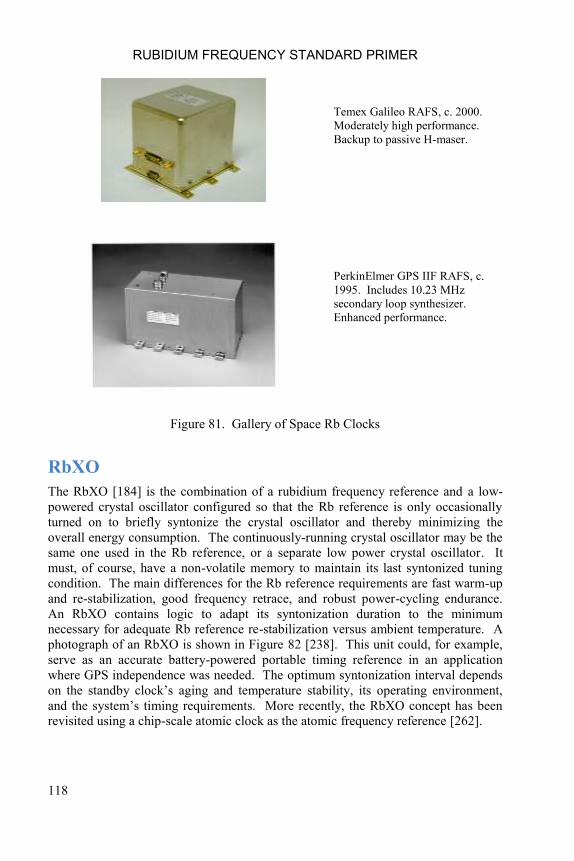
RUBIDIUM FREQUENCY STANDARD PRIMER
118
Temex Galileo RAFS, c. 2000.
Moderately high performance.
Backup to passive H-maser.
PerkinElmer GPS IIF RAFS, c.
1995. Includes 10.23 MHz
secondary loop synthesizer.
Enhanced performance.
Figure 81. Gallery of Space Rb Clocks
RbXO
The RbXO [184] is the combination of a rubidium frequency reference and a low-
powered crystal oscillator configured so that the Rb reference is only occasionally
turned on to briefly syntonize the crystal oscillator and thereby minimizing the
overall energy consumption. The continuously-running crystal oscillator may be the
same one used in the Rb reference, or a separate low power crystal oscillator. It
must, of course, have a non-volatile memory to maintain its last syntonized tuning
condition. The main differences for the Rb reference requirements are fast warm-up
and re-stabilization, good frequency retrace, and robust power-cycling endurance.
An RbXO contains logic to adapt its syntonization duration to the minimum
necessary for adequate Rb reference re-stabilization versus ambient temperature. A
photograph of an RbXO is shown in Figure 82 [238]. This unit could, for example,
serve as an accurate battery-powered portable timing reference in an application
where GPS independence was needed. The optimum syntonization interval depends
on the standby clock‟s aging and temperature stability, its operating environment,
and the system‟s timing requirements. More recently, the RbXO concept has been
revisited using a chip-scale atomic clock as the atomic frequency reference [262].
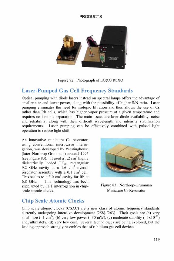
PRODUCTS
119
Figure 82. Photograph of EG&G RbXO
Laser-Pumped Gas Cell Frequency Standards
Optical pumping with diode lasers instead on spectral lamps offers the advantage of
smaller size and lower power, along with the possibility of higher S/N ratio. Laser
pumping eliminates the need for isotopic filtration and thus allows the use of Cs
rather than Rb cells, which has higher vapor pressure at a given temperature and
requires no isotopic separation. The main issues are laser diode availability, noise
and reliability, along with their difficult wavelength and intensity stabilization
requirements. Laser pumping can be effectively combined with pulsed light
operation to reduce light shift.
An innovative miniature Cs resonator,
using conventional microwave interro-
gation, was developed by Westinghouse
(later Northrop-Grumman) around 1995
(see Figure 83). It used a 1.2 cm3 highly
dielectrically loaded TE201 rectangular
9.2 GHz cavity in a 1.6 cm3 overall
resonator assembly with a 0.1 cm3 cell.
This scales to a 3.0 cm3 cavity for Rb at
6.8 GHz. This technology has been
supplanted by CPT interrogation in chip-
scale atomic clocks.
Figure 83. Northrop-Grumman
Miniature Cs Resonator
Chip Scale Atomic Clocks
Chip scale atomic clocks (CSAC) are a new class of atomic frequency standards
currently undergoing intensive development [258]-[263]. Their goals are (a) very
small size (≈1 cm3), (b) very low power (≈30 mW), (c) moderate stability (≈1x10
-11)
and, ultimately, (d) very low cost. Several technologies are being explored, but the
leading approach strongly resembles that of rubidium gas cell devices.

RUBIDIUM FREQUENCY STANDARD PRIMER
120
A fundamental factor is that tiny (≈1 mm long) cesium and rubidium gas cells with
buffer gas can produce narrow (≈1 kHz) resonances. Other enabling factors are the
use of diode lasers and coherent population trapping (CPT) interrogation, along with
MEMS (micro electro-mechanical systems) technology to batch-fabricate cells using
semiconductor technology. Coupled with low power RF and microcontroller
electronics, many of the CSAC goals have already been realized as shown in Figure
84 for the 16 cc, 120 mW Symmetricom SA.45s CSAC.
Figure 84. Symmetricom SA.45s
Chip Scale Atomic Clock
CPT Interrogation
CPT interrogation avoids the requirement for a large microwave cavity by
modulating a diode laser tuned to one of the Cs or Rb D lines with RF at one-half of
the hyperfine frequency. That produces an optical field with coherent sidebands
separated by the atomic resonance that interacts with the atoms such that the
transmitted light is a maximum when the RF frequency is at the center of the atomic
line. A frequency lock servo locks the RF frequency as in a conventional RFS, while
other digital servo loops control the cell and laser diode temperatures and the laser
wavelength and intensity.
Chip scale atomic clocks and coherent population trapping interrogation offer
attractive new opportunities for wider deployment of atomic clocks, opening up
entirely new applications for precise timing, especially in portable equipment. An
example of a commercial CPT rubidium clock is described in Reference [264].
Advanced Rubidium Clocks
The mature RFS technologies covered in this primer have a 50-year record of
improvement, and, because of their combination of performance and practicality,
will continue to be the most common form of atomic clock for the foreseeable future.
Opportunities also continue for further improvements, including the use of laser
pumping, a better understanding of aging and noise floor mechanisms, more
effective use of digital control, and the availability of new electronic components.
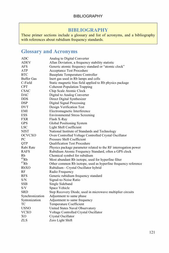
BIBLIOGRAPHY
121
BIBLIOGRAPHY These primer sections include a glossary and list of acronyms, and a bibliography
with references about rubidium frequency standards.
Glossary and Acronyms
ADC Analog to Digital Converter
ADEV Allan Deviation, a frequency stability statistic
AFS Generic atomic frequency standard or “atomic clock”
ATP Acceptance Test Procedure
BTC Baseplate Temperature Controller
Buffer Gas Inert gas used in Rb lamps and cells
C-Field Static magnetic bias field applied to Rb physics package
CPT Coherent Population Trapping
CSAC Chip Scale Atomic Clock
DAC Digital to Analog Converter
DDS Direct Digital Synthesizer
DSP Digital Signal Processing
DVT Design Verification Test
EMI Electromagnetic Interference
ESS Environmental Stress Screening
FXR Flash X-Ray
GPS Global Positioning System
LSC Light Shift Coefficient
NIST National Institute of Standards and Technology
OCVCXO Oven Controlled Voltage Controlled Crystal Oscillator
PC Pressure Shift Coefficient
QTP Qualification Test Procedure
Rabi Rate Physics package parameter related to the RF interrogation power
RAFS Rubidium Atomic Frequency Standard, often a GPS clock
Rb Chemical symbol for rubidium 85Rb Most abundant Rb isotope, used for hyperfine filter 87Rb Other common Rb isotope, used as hyperfine frequency reference
RbXO Rubidium - Crystal Oscillator hybrid
RF Radio Frequency
RFS Generic rubidium frequency standard
S/N Signal-to-Noise Ratio
SSB Single Sideband
S/V Space Vehicle
SRD Step Recovery Diode, used in microwave multiplier circuits
Synchronization Adjustment to same phase
Syntonization Adjustment to same frequency
TC Temperature Coefficient
USNO United States Naval Observatory
VCXO Voltage Controlled Crystal Oscillator
XO Crystal Oscillator
ZLS Zero Light Shift

RUBIDIUM FREQUENCY STANDARD PRIMER
122
Bibliography
Note: This bibliography is organized by topic, sorted by date, and numbered
consecutively. Some of these items are also referenced by number in the main text.
General Atomic Clocks
[1] C. Steiner, “Atomic Clocks”, Parts I-III, Frequency, March-May 1968.
[2] H. Hellwig, “Areas of Promise for the Development of Future Primary
Frequency Standards”, Proceedings of the 24th
Annual Symposium on
Frequency Control, pp. 246-258, April 1970.
[3] C. Audoin and J. Vanier, “Atomic Frequency Standards and Clocks”, J. Phys.
E., Vol. 9, pp. 697-720, 1976.
[4] H. Hellwig, K.M. Evenson and D.J. Wineland, “Time, Frequency and Physical
Measurement”, Physics Today, pp. 23-30, December 1978.
[5] C. Audoin and J. Vanier, “Atomic Frequency Standards, a Critical Review”, c.
1980.
[6] J. Vanier and C. Audoin, The Quantum Physics of Atomic Frequency
Standards, Adam Hilger, Bristol and Philadelphia, Volume 2, Chapter 7, ISBN
0-85274-433-1, 1989.
[7] D.B Sullivan, D.W Allan, D.A. Howe and F.L.Walls (Editors),
"Characterization of Clocks and Oscillators", NIST Technical Note 1337, U.S.
Department of Commerce, National Institute of Standards and Technology,
March 1990.
[8] A.O. McCoubrey, “History of Atomic Frequency Standards: A Trip Through
20th
Century Physics”, Proceedings of the 1996 IEEE International Frequency
Control Symposium, pp. 12251241, June 1996.
[9] C. Audoin and B. Guinot, The Measurement of Time, Cambridge University
Press, Cambridge, U.K., ISBN 0-521-80080-3, 2001.
[10] F.G. Major, The Quantum Beat: Principles and Applications of Atomic Clocks,
2nd
Edition, Springer-Science, 2007, ISBN 978-0-387-69533-4.
History
[11] N.F. Ramsey, “History of Early Atomic Clocks”, Metrologia, Vol. 42 S1,
2005.
[12] P. Forman, “Atomic Clocks: Preview of an Exhibit at the Smithsonian,
Proceedings of the 36th
Annual Symposium on Frequency Control, pp. 220-222,
June 1982.
Early Scientific Papers
[13] Bitter, Physical Review, Vol. 76, pp. 883-885, 1949.
[14] Brossel and A. Kastler, C.R. Acad. Sci. (Paris), Vol. 229, p.1213, 1949.
[15] R.H. Dicke, Physical Review, Vol. 89, pp. 472-473, 1953.
[16] R.H. Dicke, “Atomic and Molecular Frequency Standards, Proceedings of the
10th
Annual Symposium on Frequency Control, p. 259, 1956.

BIBLIOGRAPHY
123
[17] P.L. Bender, E.C. Beaty and A.R. Chi, “Optical Detection of Narrow Rb87
Hyperfine Absorption Lines”, Physical Review Letters, Vol. 1, No. 9, pp. 311-
313, November 1958.
General RFS Theory
[18] A.L. Bloom, “Optical Pumping”, Scientific American, pp. 72-80, XXX 1960.
[19] M. Arditi and T.R. Carver, “Pressure, Light and Temperature Shifts in Optical
Detection of 0-0 Hyperfine Resonance of Alkali Metals”, Physical Review,
Vol. 124, No. 3, pp. 800-809. November 1961.
[20] A. Kastler, “Displacement of Energy Levels of Atoms by Light”, J. Op. Soc.
Am., Vol. 53, No. 8, pp. 902-910, August 1963.
[21] M. Arditi and T.R. Carver, “Hyperfine Relaxation of Optically Pumped Rb87
Atoms in Buffer Gases”, Physical Review, Vol. 136, pp. A643-A649,
November 1964.
[22] R. Bernheim, Optical Pumping, W.A. Benjamin, New York, 1965.
[23] R.W. Frank, R.P. Kenschaft, R.A. Mortenson, W.J. Riley and H.P.
Stratemeyer, “Design Concepts Study for an Aerospace Rubidium Standard”,
General Radio Company, Bolton, MA 01740, October 1969.
[24] B.E. Blair, Editor, Time and Frequency: Theory and Fundamentals, NBS
Monograph 140, U.S. Department of Commerce, May 1974.
[25] G. Missout and J. Vanier, “Some Aspects of the Theory of Passive Rubidium
Frequency Standards”, Canadian Journal of Physics, Vol. 53, No. 11, pp.
1030-1043, 1975.
[26] A. Risley and G. Busca, “Effect of Line Inhomogeneity on the Frequency of
Passive Rb87
Frequency Standards”, Proceedings of the 32nd
Annual
Symposium on Frequency Control, pp. 506-513, June 1978.
[27] A.S. Risley. “Final Report on the Microwave Power and Lamp Temperature
Dependence of the Frequency of a Passive Rb87
Frequency Standard”, National
Bureau of Standards, Boulder, CO, c. 1977.
[28] T.C. English, E. Jechart and T.M. Kwon, “Elimination of the Light Shift in
Rubidium Gas Cell Frequency Standards Using Pulsed Optical Pumping”,
Proceedings of the 10th
Annual Precise Time and Time Interval (PTTI)
Applications and Planning Meeting, Greenbelt, MD, pp. 147-168, November
1978.
[29] J. Vanier and L. Bernier, “On the Signal to Noise Ratio and Short Term
Stability of Passive Rubidium Frequency Standards”, Laboratorire
D‟Electronique Quantique, Departement de Genie Electrique, Universite Laval,
February 1981.
[30] J. Vanier, “Light Shifts in Passive Rubidium Frequency Standards Using
Hyperfine Filtering”, Final Report, Universite Laval, April 1981.
[31] J. Vanier, R. Kunski, P. Paulin, J.V. Savard, M. Tetu and N. Cyr, “On the Light
Shift and Buffer Gas Shift in Passive Rubidium Frequency Standards”,
Proceedings of the 36th
Annual Symposium on Frequency Control, pp. 348-354,
June 1982.

RUBIDIUM FREQUENCY STANDARD PRIMER
124
[32] C. Audoin, J. Viennet, N. Cyr and J. Vanier, “Influence of Modulation
Frequency in Rubidium Cell Frequency Standards”, Proceedings of the 14th
Annual Precise Time and Time Interval (PTTI) Applications and Planning
Meeting, Greenbelt, MD, pp. 87-110, November-December 1982.
[33] P. Tremblay, N. Cyr and Michel Tetu, “Evaluation of the Performance of
Passive Rubidium Frequency Standards Using Cavity Operated in Mode TE011,
TE111, and TE101”, Proceedings of the 38th
Annual Symposium on Frequency
Control, pp. 406-415, June 1984.
[34] P. Tremblay, N. Cyr and Michel Tetu, “Pumping Light Intensity Transmitted
through an Inhomogeneously Broadened Line System: Application to Passive
Rubidium Frequency Standards”, Can. J. Physics, Vol. 63, No. 12, December
1985.
Early RFS Research and Development
[35] T.R. Carver, “Rubidium Oscillator Experiments”, Proceedings of the 11th
Annual Symposium on Frequency Control, pp. 307-XXX, XXX 1957.
[36] M. Arditi, “Gas Cell Atomic Clocks Using Buffer Gases and Optical
Orientation”, Proceedings of the 12th
Annual Symposium on Frequency
Control, pp. 606-622, April 1958.
[37] J.M. Andres, D.J. Farmer and G.T. Inouye, “Design Studies for a Rubidium
Gas Cell Frequency Standard”, IRE Trans. Mil. Electron., MIL-3, pp. 178-183,
October 1959.
[38] M. Arditi, “Evaluation of ITT Breadboard Gas Cell Frequency Standard”,
Proceedings of the 13th
Annual Symposium on Frequency Control, pp. 655-667,
May 1959.
[39] M. Arditi, IRE Trans. Mil. Electron., MIL-4, pp. 22-XX, 1960.
[40] R.J. Carpenter, E.C. Beaty, P.L. Bender, S. Saito and R.O. Stone, “A Prototype
Rubidium Vapor Frequency Standard”, IRE Trans. Instrum., Vol. I-9, pp. 132-
135, September 1960.
[41] M. Arditi, “Frequency Control by Gas Cell Standards – Fundamental Problems
in the Light of Recent Experimental Results”, Proceedings of the 15th
Annual
Symposium on Frequency Control, pp. 181-202, April 1961.
[42] M. Arditi and T.R. Carver, “The Principles of the Double Resonance Method
Applied to Gas Cell Frequency Standards”, Proc. IEEE, pp. 190-202, January
1963.
[43] D.J. Farmer, “Performance and Application of Gas Cell frequency Standards”,
Proceedings of the 17th Annual Symposium on Frequency Control, pp. 449-
XXX, April 1963.
[44] M.E. Packard and B.E. Swartz, “The Optically Pumped Rubidium Vapor
Frequency Standard”, IRE Trans. Instrum., I-11, pp. 215-223, December 1962.
[45] A.R. Chi, J.H. Roeder, S.C. Wardrip and B. Kruger, “Long-Term Stability
Frequency Stability Measurement of Rubidium Gas Cell Frequency
Standards”, Proceedings of the 22nd
Annual Symposium on Frequency Control,
pp. 592-604, XXXX 1968.
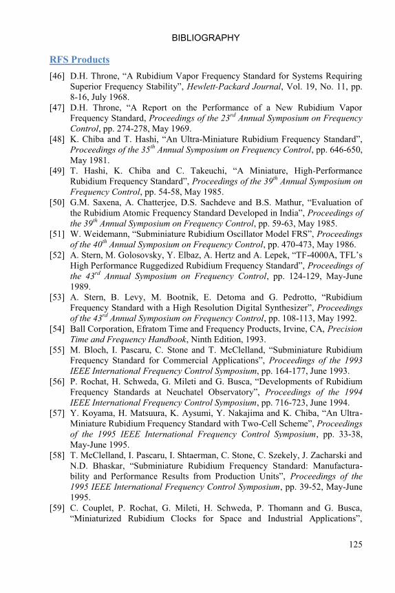
BIBLIOGRAPHY
125
RFS Products
[46] D.H. Throne, “A Rubidium Vapor Frequency Standard for Systems Requiring
Superior Frequency Stability”, Hewlett-Packard Journal, Vol. 19, No. 11, pp.
8-16, July 1968.
[47] D.H. Throne, “A Report on the Performance of a New Rubidium Vapor
Frequency Standard, Proceedings of the 23rd
Annual Symposium on Frequency
Control, pp. 274-278, May 1969.
[48] K. Chiba and T. Hashi, “An Ultra-Miniature Rubidium Frequency Standard”,
Proceedings of the 35th
Annual Symposium on Frequency Control, pp. 646-650,
May 1981.
[49] T. Hashi, K. Chiba and C. Takeuchi, “A Miniature, High-Performance
Rubidium Frequency Standard”, Proceedings of the 39th
Annual Symposium on
Frequency Control, pp. 54-58, May 1985.
[50] G.M. Saxena, A. Chatterjee, D.S. Sachdeve and B.S. Mathur, “Evaluation of
the Rubidium Atomic Frequency Standard Developed in India”, Proceedings of
the 39th
Annual Symposium on Frequency Control, pp. 59-63, May 1985.
[51] W. Weidemann, “Subminiature Rubidium Oscillator Model FRS”, Proceedings
of the 40th
Annual Symposium on Frequency Control, pp. 470-473, May 1986.
[52] A. Stern, M. Golosovsky, Y. Elbaz, A. Hertz and A. Lepek, “TF-4000A, TFL‟s
High Performance Ruggedized Rubidium Frequency Standard”, Proceedings of
the 43rd
Annual Symposium on Frequency Control, pp. 124-129, May-June
1989.
[53] A. Stern, B. Levy, M. Bootnik, E. Detoma and G. Pedrotto, “Rubidium
Frequency Standard with a High Resolution Digital Synthesizer”, Proceedings
of the 43rd
Annual Symposium on Frequency Control, pp. 108-113, May 1992.
[54] Ball Corporation, Efratom Time and Frequency Products, Irvine, CA, Precision
Time and Frequency Handbook, Ninth Edition, 1993.
[55] M. Bloch, I. Pascaru, C. Stone and T. McClelland, “Subminiature Rubidium
Frequency Standard for Commercial Applications”, Proceedings of the 1993
IEEE International Frequency Control Symposium, pp. 164-177, June 1993.
[56] P. Rochat, H. Schweda, G. Mileti and G. Busca, “Developments of Rubidium
Frequency Standards at Neuchatel Observatory”, Proceedings of the 1994
IEEE International Frequency Control Symposium, pp. 716-723, June 1994.
[57] Y. Koyama, H. Matsuura, K. Aysumi, Y. Nakajima and K. Chiba, “An Ultra-
Miniature Rubidium Frequency Standard with Two-Cell Scheme”, Proceedings
of the 1995 IEEE International Frequency Control Symposium, pp. 33-38,
May-June 1995.
[58] T. McClelland, I. Pascaru, I. Shtaerman, C. Stone, C. Szekely, J. Zacharski and
N.D. Bhaskar, “Subminiature Rubidium Frequency Standard: Manufactura-
bility and Performance Results from Production Units”, Proceedings of the
1995 IEEE International Frequency Control Symposium, pp. 39-52, May-June
1995.
[59] C. Couplet, P. Rochat, G. Mileti, H. Schweda, P. Thomann and G. Busca,
“Miniaturized Rubidium Clocks for Space and Industrial Applications”,

RUBIDIUM FREQUENCY STANDARD PRIMER
126
Proceedings of the 1995 IEEE International Frequency Control Symposium,
pp. 53-59, May-June 1995.
[60] T. McClelland, I. Pascaru, I. Shtaerman, C. Stone, C. Szekely, J. Zacharski and
N.D. Bhaskar, “Subminiature Rubidium Frequency Standard: Performance
Improvements”, Proceedings of the 1996 IEEE International Frequency
Control Symposium, pp. 1011-1016, June 1996.
[61] K. Suzuki, Y. Abe, N. Ishihara, H. Kudoh and S. Fukugawa, “Small-Sized
Rubidium Oscillator”, Proceedings of the 1998 IEEE International Frequency
Control Symposium, pp. 73-79, May 1998.
[62] J. Ho, I. Pascaru, C. Stone and T. McClelland, “New Rubidium Frequency
Standard Designa for Telecommunications Applications”, Proceedings of the
1998 IEEE International Frequency Control Symposium, pp. 80-83, May 1998.
[63] W. J. Riley, “A Modern Militarized Rubidium Frequency Standard”,
Microwave Journal, May 2002.
[64] Y. Koyama, H. Matsuura, K. Atsumi, K. Nakamuta, M. Sakai and I.
Maruyama, An Ultra-Miniature Rubidium Frequency Standard”, Proceedings
of the 2000 IEEE International Frequency Control Symposium, pp. 694-699,
June 2000.
Rubidium
[65] Daniel A. Steck. "Rubidium-87 D Line Data", Los Alamos National Laboratory
Technical report LA-UR-03-8638, September 2001.
[66] It has been reported that a lack of the mineral rubidium may cause: depression,
decreased cancer resistance, decreased cell PH, cell dehydration, increased
enzyme toxicity, decreased glucose tolerance, decreased peroxides elimination.
See http://www.4alw.com/liquid-minerals/rubidium.
RFS Environmental Sensitivity
[67] W. J. Riley, “The Physics of the Environmental Sensitivity of Rubidium Gas
Cell Atomic Frequency Standards”, IEEE Transactions on Ultrasonics,
Ferroelectrics and Frequency Control, Vol. 39, No. 2, pp. 232-240, March
1992.
[68] M. Huang, C. M. Klimcak, and J. C. Camparo, "Vapor-Cell Clock Frequency
and Environmental Pressure: Resonance-Cell Volume Changes", Proceedings
of the 2010 IEEE International Frequency Control Symposium, pp. 208-211,
June 2010.
RFS Testing
[69] T. J. Lynch, W. J. Riley and J. R. Vaccaro, “The Testing of Rubidium
Frequency Standards”, Proceedings of the 43rd
Annual Symposium on
Frequency Control, pp. 257-262, May 1989.
[70] J. Vanier, et. al., “Aging, Warm-up Time and Retrace: Important
Characteristics of Standard Frequency Generators”, Proceedings of the 1992
IEEE Frequency Control Symposium, pp. 807-XXX, June 1992.

BIBLIOGRAPHY
127
[71] T. Lynch and W. Riley, “Tactical Rubidium Frequency Standard (TRFS)”,
RADC-TR-87-166, Final Technical Report, Oct. 1987.
[72] MIL-STD-454, “Standard General Requirements for Electronic Equipment”.
[73] MIL-STD-810, “Environmental Test Methods”.
[74] MIL-STD-461, “Electromagnetic Interference Characteristics, Requirements
For Equipment”.
[75] MIL-E-5400, “Electronic Equipment, Airborne, General Specification For.”
[76] MIL-T-5422, “Testing, Environmental, Airborne Electronic And Associated
Equipment.”
[77] MIL-E-16400, “Electronic Equipment, Naval Ship and Shore, General
Specification”.
[78] MIL-E-4158, “Electronic Equipment, Ground, General Requirements For”.
[79] DOD-E-8983, “Electronic Equipment, Aerospace, Extended Space
Environment, General Specification For”.
[80] MIL-STD-1540, “Test Requirements for Space Vehicles.
[81] MIL-STD-1541, “Electromagnetic Compatibility Requirements for Space
Systems”.
[82] MIL-C-45662, “Calibration System Requirements”.
[83] MIL-O-55310B, “Military Specification, Oscillators, Crystal, General
Specification For,” 10 May 1988.
[84] MIL-STD-202, “Test Methods for Electronic and Electrical Component Parts.”
[85] MIL-STD-462, “Electromagnetic Interference Characteristics, Measurement
of”.
[86] MIL-STD-704, “Platform Electrical Power Characteristics”.
[87] MIL-STD-1275, “Characteristics of 28VDC Electrical System in Military
Vehicles”.
[88] ARNIC Report 413, “Guidance for Aircraft and Electrical Power Utilization
and Transient Protection.” Aeronautical Radio, Inc., Dec. 1976.
[89] ASTM 346-64, “Standard Methods of Test of Magnetic Shielding.” American
Society for Testing and Materials.
[90] W. Riley and J. Vaccaro, “Rubidium-Crystal Oscillator (RbXO) Development
Program,” U.S. Army LABCOM R&D Technical Report SLCET-TR-84-0410F,
April 1986.
[91] MIL-STD-2164(EC), “Environmental Stress Screening Process for Electronic
Equipment”.
[92] NAVMAT P-9492, “Navy Manufacturing Screening Program”.
[93] A.J. Curtis and R.D. McKain, “A Quantitative Method of Tailoring Input
Spectra for Random Vibration Screens,” J. Env. Sci., Sept. - Oct. 1987.
[94] R.G. Lambert, “Case Histories of Selection Criteria for Random Vibration
Screening”, Inst. Env. Sci. Workshop Proc., Sept. 1984.
[95] W. Weidemann, “Application Critical Parameters for Rubidium Standards”,
Proceedings of the 1998 IEEE International Frequency Control Symposium,
pp. 84-87, May 1998.
[96] D. Watts, F. Li, F. Vu, W.F. Cashin and T.C. English, “Specifying Commercial
Atomic Frequency Standards Using Statistics”, Proceedings of the 1996 IEEE
International Frequency Control Symposium, pp. 1023-1031, June 1996.

RUBIDIUM FREQUENCY STANDARD PRIMER
128
Rb Lamps
[97] W.E. Bell, A.L. Bloom and J. Lynch, “Alkali Metal Vapor Spectral Lamps”,
Review of Scientific Instruments, Vol. 32, No. 6, pp. 688-692, June 1961.
[98] R.G. Brewer, “High Intensity Low Noise Rubidium Light Source”, Review of
Scientific Instruments, Vol. 32, No. 12, pp. 1356-1358, December 1961.
[99] N. Oura, N. Kuramochi, S. Naritsuka and T. Hayashi, :Composite-Type 87Rb
Optical Pumping Light Source for the Rubidium Frequency Standard”,
Proceedings of the 13th
Annual Precise Time and Time Interval (PTTI)
Applications and Planning Meeting, Washington, DC, pp. 803-815, December
1981.
[100] C. H. Volk, R.P. Frueholtz, T.C. English, T.J. Lynch and W.J. Riley, “Lifetime
and Reliability of Rubidium Discharge Lamps for Use in Atomic Frequency
Standards”, Proceedings of the 38th
Annual Frequency Control Symposium,
Philadelphia, PA, pp. 387-400, May 1984.
[101] R.A. Cook and R.P. Frueholtz, “An Improved Rubidium Consumption Model
for Discharge Lamps Used in Rubidium Frequency Standards”, Proceedings
of the 42th
Annual Frequency Control Symposium, Baltimore, MD, pp. 525-
531, June 1988.
[102] J. Comparo and R. Mackay, “A Mechanism of Rubidium Clock Degradation:
Ring-Mode to Red-Mode Transition in RF-Discharge Lamps”, Proceedings of
the 2007 IEEE International Frequency Control Symposium, Geneva, pp. 45-
48, May-June 2007.
Lamp Exciters
[103] R. Shaw, “Spontaneously Generated Ion Acoustic Waves in a Weakly Ionized
Plasma”, MS Thesis, Cornell University, Ithaca, NY, September 1964. .
[104] W.J. Riley, “Power Supply Circuit for an Alkali Vapor Spectral Lamp” U.S.
Patent No. 4,721,890, January 1988.
[105] Performance Analysis, Lamp Exciter, FP0034, EG&G Frequency Products,
August 1990.
Harmonic Multipliers
[106] C. Wenzel, “New Topology Multiplier Generates Odd Harmonics”, RF
Design, Vol. 10, No. 7, pp. 31-34, July 1987.
[107] B. Sadowski, “Low Additive Noise Frequency Tripler”, RF Design, pp. 32-35,
May 2007.
SRD Multipliers
[108] H.T. Friis, “Analysis of Harmonic Generator Circuits for Step Recovery
Diodes” Proceedings of the IEEE, Vol. 55, No. 7, pp. 1192-1194, July 1967.
[109] A. Shipow, “Harmonic Generators”, Microwave Journal, February 1978.
[110] “Harmonic Generation Using Step Recovery Diodes and SRD Modules”,
Application Note 920, Hewlett-Packard Company.

BIBLIOGRAPHY
129
GPS Rb Clocks
[111] D.E. Ringer, J. Gandy and E. Jechart, “Spaceborne Rubidium Frequency
Standard for NAVSTAR GPS”, Proceedings of the 7th
Annual Precise Time
and Time Interval (PTTI) Applications and Planning Meeting, pp. 671-696,
December 1975.
[112] Final Report, “Design for a Rubidium Frequency Standard”, General Radio
Company, Bolton, MA 01740 , February, 1976.
[113] “Design for a Rubidium Frequency Standard for the GPS Program”, Final
Report, Rockwell Contract No. M5N3DGS-649024D, February 1976.
[114] Progress Report, “GPS Rubidium Frequency Standard”, EG&G Electronic
Components, Salem MA 01970, February 1980.
[115] “Preliminary Design Concept Review, Contract No. MOJ3BGR-484107E”,
EG&G Electronic Components, Salem MA 01970, May 1980.
[116] Technical Report, “Program Progress Review #2, Phase 1 Breadboard
Development, Rubidium Frequency Standard”, EG&G Electronic
Components, Salem MA 01970, September 1980.
[117] Technical Report, “Program Progress Review #3, Phase 1 Breadboard
Development, Rubidium Frequency Standard”, EG&G Electronic
Components, Salem MA 01970, November 1980.
[118] Technical Report, “Program Progress Review #4, Phase 1 Breadboard
Development, Rubidium Frequency Standard”, EG&G Electronic
Components, Salem MA 01970, January 1981.
[119] Performance Analysis, “GPS Rubidium Frequency Standard”, EG&G
Electronic Components, Salem, MA 01970, October 1981.
[120] W. J. Riley, “A Rubidium Clock for GPS”, Proceedings of the 13th
Annual
Precise Time and Time Interval (PTTI) Applications and Planning Meeting,
Washington, DC, pp. 609-630, December 1981.
[121] Technical Report, “Critical Design Review, GPS Rubidium Frequency
Standard”, EG&G Electronic Components, Salem MA 01970, May 1982.
[122] T. J. Lynch and W. J. Riley, “Test Results for Prototype GPS Rubidium
Clocks, Proceedings of the 15th
Annual Precise Time and Time Interval
(PTTI) Applications and Planning Meeting, Washington, DC, pp. 269-280,
December 1983.
[123] Final Report, “140 Day Stability Test, EG&G GPS RFS Prototype #1”, NBS
Test No. 801590, EG&G Electronic Components, Salem MA 01970, February
1983.
[124] Qualification Level Test Report, “GPS RFS”, EG&G Frequency Products,
Salem, MA 01970, March 1983.
[125] Final Technical Report, “EG&G GPS RFS Continuation Program”, EG&G
Electronic Components, Salem MA 01970, June 1985.
[126] S. Goldberg, T. J. Lynch and W. J. Riley, “Further Test Results for Prototype
GPS Rubidium Clocks, Proceedings of the 17th
Annual Precise Time and
Time Interval (PTTI) Applications and Planning Meeting, Washington, DC,
pp. 145-155, December 1985.

RUBIDIUM FREQUENCY STANDARD PRIMER
130
[127] F. Danzy and W. J. Riley, “Stability Test Results for GPS Rubidium Clocks,
Proceedings of the 19th Annual Precise Time and Time Interval (PTTI)
Applications and Planning Meeting, Redondo Beach, CA, pp. 267-274,
December 1987.
[128] Acceptance Test Report, “GE GPS Rubidium Frequency Standards S/N 3 &
4”, EG&G Frequency Products, Salem, MA 01970, August 1989.
[129] W. J. Riley, “Rubidium Atomic Frequency Standards for GPS Block IIR,
Proceedings of the 22nd Annual Precise Time and Time Interval (PTTI)
Applications and Planning Meeting, Vienna, VA, pp. 221-230, December
1990.
[130] “Input Current Time Profile Analysis, Dynamic Input Impedance, GPS Block
IIR RAFS”, EG&G Frequency Products, Salem, MA 01970, March 1990.
[131] Test Report, “Transient Radiation Test, Crystal Oscillator, GPS Block IIR
RAFS”, EG&G Frequency Products, Salem, MA 01970, April 1990.
[132] Test Report, “Transient Radiation Test, Output Amplifier, GPS Block IIR
RAFS”, EG&G Frequency Products, Salem, MA 01970, April 1990.
[133] Critical Design Review, GPS Block IIR Phase 2, “Rubidium Atomic
Frequency Standard”, EG&G Frequency Products, Salem, MA 01970, June
1990.
[134] Manufacturing Readiness Review, GPS Block IIR Phase 2, “Rubidium Atomic
Frequency Standard”, EG&G Frequency Products, Salem, MA 01970, August
1990.EG&G No. FP0043, “Qualification-Level Test Report, GPS Block IIR
RAFS”, EG&G Frequency Products, Salem, MA 01970, June 1991.
[135] W. J. Riley, “Rubidium Atomic Frequency Standards for GPS Block IIR,
Proceedings of the 6th
European Frequency and Time Forum, Noordwijk, NL,
pp. 231-238, March 1992.
[136] W. J. Riley, “Rubidium Atomic Frequency Standards for GPS Block IIR,
Proceedings of the 5th
Technical Meeting of the Satellite Division of the
Institute of Navigation, Albuquerque, NM, pp. 537-545, September 1992.
[137] Qualification Test Report, “GPS Block IIR Rubidium Atomic Frequency
Standard”, EG&G Rubidium Products, Salem, MA 01970, May 1994.
[138] Test Report, “Frequency Retrace Test of GPS Block IIR RAFS EDM1”,
EG&G Rubidium, Salem, MA 01970, September 1994.
[139] W. J. Riley, “Early Stability Test Results for GPS Block IIR Rubidium
Clocks, Proceedings of the 5th Symposium on Frequency Standards &
Metrology, Woods Hole, MA, October 1995, pp. 403-405.
[140] Technical Interchange Meeting, “RAFS Frequency Jumps”, EG&G
Frequency Products, Salem, MA 01970, August 1995.
[141] “Interpretation of GPS Block IIR RAFS Monitor Signals”, EG&G Rubidium,
Salem, MA 01970, March 1996.
[142] Design Concept, GPS Block IIF Rubidium Frequency Standard, EG&G
Frequency Products, Salem, MA 01970, September 1996.
[143] Test Report, RAFS Warm-up Test, EG&G Frequency Products, Salem, MA
01970, November 1996.
[144] Operations Manual, GPS Block IIR Rubidium Atomic Frequency Standard,
EG&G Frequency Products, Salem, MA 01970, November 1996.

BIBLIOGRAPHY
131
[145] Breadboard Report, “RFS-IIF Rubidium Frequency Standard”, EG&G
Frequency Products, Salem, MA 01970, December 1996.
[146] Test Report, “RFS-IIF Secondary Loop Synthesizer Flash X-Ray Test”,
EG&G Frequency Products, Salem, MA 01970, March 1997.
[147] Test Report, “RFS-IIF Prototype Evaluation”, EG&G Frequency Products,
Salem, MA 01970, June 1997.
[148] Test Report, “RFS-IIF Prototype Radiation Test”, EG&G Frequency Products,
Salem, MA 01970, September 1997.
[149] Test Report, “RFS-IIF EDU Initial Functional Test”, EG&G Frequency
Products, Salem, MA 01970, September 1997.
[150] Critical Design Review, GPS Block IIF, “Rubidium Frequency Standard”,
EG&G Frequency Products, Salem, MA 01970, November 1997.
[151] W.J. Riley, “Early In-Orbit Performance of GPS Block IIR Rubidium Clocks,
Proceedings of the 29th Annual Precise Time and Time Interval (PTTI)
Applications and Planning Meeting, Long Beach, CA, pp. 213-220,
November 1997.
[152] Qualification Test Report, “AFTR RFS, EG&G P/N 603-9598”, EG&G
Optoelectronics, Salem MA 01970, July 1998.
[153] Final Report, “SVN43 TKS Event Investigation”, EG*G Frequency Products,
Salem, MA 01970, July 1998.
[154] T.J. Lynch, K.D. Lyon, W.J. Riley and J.R. Vaccaro, “A Rubidium Clock for
GPS Block IIF”, April 1999 (unpublished).
[155] R.F. Dupuis, T.J. Lynch and J.R. Vaccaro, “Rubidium Frequency Standard for
the GPS IIF Program and Modifications for the RAFSMOD Program”,
Proceedings of the 2008 IEEE International Frequency Control Symposium,
Honolulu, HI, pp. 655-660, May 2008.
Space RFS (Non-GPS)
[156] R.W. Frank, R.P. Kenschaft, R.A Mortenson, W.J. Riley and H.P.
Stratemeyer, “Design Concepts for an Aerospace Rubidium Standard”,
General Radio Company, October 1969.
[157] Final Report, NASA Contract NAS 9-5425, Part II, “Rubidium Spacecraft
Atomic Timing System”, General Radio Company, W. Concord, MA 01742,
December, 1969.
[158] Design Study, “Milstar Feasibility Study, Rubidium Interface Unit”, EG&G
Frequency Products, Salem, MA 01970, January 1998.
MIL (Tactical) RFS
[159] M.E. Frerking and D.E. Johnson, “Rubidium Frequency and Time Standard
for Military Environment”, Proceedings of the 26th
Annual Symposium on
Frequency Control, pp. 216-222, June 1972.
[160] Final Technical Report, Rome Air Development Center, Contract No.
F19628-82-C-0055, “Phase 2A Bench Model Development, Tactical
Rubidium Frequency Standard”, EG&G Frequency Products, Salem, MA
01970, December 1982.

RUBIDIUM FREQUENCY STANDARD PRIMER
132
[161] W.J. Riley, “A Rubidium Clock for Seek-Talk”, Proceedings of the 14th
Annual Precise Time and Time Interval (PTTI) Applications and Planning
Meeting, pp. 141-154, December 1982.
[162] Final Technical Report, Rome Air Development Center, Contract No.
F19628-82-C-0055, “Phase 2B Prototype Redesign, Tactical Rubidium
Frequency Standard”, EG&G Frequency Products, Salem, MA 01970, January
1983.
[163] T.M. Kwon, B.C. Grover and H.E. Williams, “Rubidium Frequency Standard
Study”, RADC-TR-83-230, Final Technical Report, Rome Air Development
Center, October 1983.
[164] T.M Kwon, R. Dagle, W. Debley, H. Dellamano, T. Hahn, J. Horste, L.K.
Lam, R. Magnuson and T. McClellan, Proceedings of the 16th
Annual Precise
Time and Time Interval (PTTI) Applications and Planning Meeting, pp. 143-
155, November 1984.
[165] Instruction Manual, “Model RFS-10 Rubidium Frequency Standard”, EG&G
Frequency Products, Salem MA 01970, January 1985.
[166] H. Fruehauf, W. Weidemann, C. Colson, S. Stein, T. English, H. Vorwerk,
and R. Paul, “Militarized Rubidium Oscillator”, RADC-TR-85-23, Final
Technical Report, Rome Air Development Center, April 1985.
[167] Qualification Test Report, “EG&G Model RFS-10-7 Rubidium Frequency
Standard”, EG&G Frequency Products, Salem, MA 01970, December 1985.
[168] Final Technical Report, Hanscom Air Force Base Contract No. F19628-83-
0175, “Tactical Rubidium Frequency Standard (TRFS)”, EG&G Frequency
Products, Salem, MA 01970, December 1986.
[169] T.M Kwon, T. Hahn, R. Dagle, J. Horste, and T. McClellan, RADC-TR-87-
140, Final Technical Report, Rome Air Development Center, September
1987.
[170] T.J. Lynch and W.J. Riley, RADC-TR-87-166, Final Technical Report,
“Tactical Rubidium Frequency Standard”, Rome Air Development Center,
EG&G Frequency Products, Salem, MA 01970, October 1987.
[171] Reliability Prediction, “SCOTT RFS-20 Rubidium Frequency Standard”,
EG&G Frequency Products, Salem MA 01970, August 1988.
[172] Radiation Test Report, “EG&G Model RFS-10-102, Regency Net Rubidium
Frequency Standard”, EG&G Frequency Products, Salem MA 01970, April
1988.
[173] Qualification Test Report, “SCOTT RFS-20 Rubidium Frequency Standard”,
EG&G Frequency Products, Salem MA 01970, August 1988.
[174] Technical Information, “Model RFS-10-7 Rubidium Frequency Standard”,
EG&G Frequency Products, Salem MA 01970, June 1989.
[175] Test Report, “Environmental Stress Screening (ESS), EG&G Model RFS-10-
7 Rubidium Frequency Standard”, EG&G Frequency Products, Salem, MA
01970, September 1989.
[176] User Manual, “Modular Intelligent Frequency, Time and Time Interval
(MIFTTI) Subsystem”, EG&G Frequency Products, Salem, MA 01970,
March 1990.

BIBLIOGRAPHY
133
[177] Test Report, “Vibration Testing of RFS-10 Rubidium Frequency Standard”,
EG&G Rubidium Products, Salem, MA 01970, October 1994.
[178] T.J. Lynch and J.R. Vaccaro, “Ultrafast Warm-up Rubidium Reference”,
Proceedings of the 1996 IEEE International Frequency Control Symposium,
Honolulu, HI, pp. 993-1001, June 1996.
[179] Qualification Test Report, “RFS-10-7 LN Combat Direction Finder Rubidium
Frequency Standard”, EG&G Optoelectronics, Salem MA 01970, September
1998.
RbXO
[180] J.R. Vig and V.J. Rosati, “The Rubidium-Crystal Oscillator Hybrid
Development Program”, Proceedings of the 16th
Annual Precise Time and
Time Interval (PTTI) Applications and Planning Meeting, pp. 157-165,
November 1984.
[181] Instruction Manual, “RbXO Demonstrator Unit”, EG&G Frequency Products,
Salem, MA 01970, December 1985.
[182] Research and Development Technical Report, US Army Laboratory
Command, Contract No. SLCET-TR-84-0410-F, “Rubidium-Crystal Oscillator
(RbXO) Development Program”, EG&G Electronic Components, Salem, MA
01970, April 1986.
[183] W. J. Riley and J. R. Vaccaro, “A Rubidium-Crystal Oscillator (RbXO)”,
Proceedings of the 40th
Annual Frequency Control Symposium, Philadelphia,
PA, pp. 452-464, May 1986.
[184] W. J. Riley and J. R. Vaccaro, “A Rubidium-Crystal Oscillator (RbXO)”,
IEEE Transactions on Ultrasonics, Ferroelectrics and Frequency Control,
Vol. UFFC-34, No. 6, pp. 612-618, November 1987.
[185] Semiannual Progress Report #1, Chip-Scale Atomic Clock, Defense
Advanced Research Projects Agency (DARPA) Contract No. NBCHC020050,
March 2003.
[186] Semiannual Progress Report #2,Chip-Scale Atomic Clock, Defense Advanced
Research Projects Agency (DARPA) Contract No. NBCHC020050, August
2003.
[187] R. Lutwak, D. Emmons, T. English, W. Riley, A. Duwel, M. Varghese, D. K.
Serkland and G. M. Peake, “The Chip-Scale Atomic Clock - Recent
Development Progress”, Proceedings of the 35th
Annual Precise Time and
Time Interval (PTTI) Applications and Planning Meeting, San Diego, CA,
December 2003.
[188] Semiannual Progress Report #3,Chip-Scale Atomic Clock, Defense Advanced
Research Projects Agency (DARPA) Contract No. NBCHC020050, February
2004.
Rb Signal Parameters
[189] Claude Audoin, Vincent Candelier, and Noel Dimarcq‟s, “A Limit to the
Frequency Stability of Passive Frequency Standards Due to an

RUBIDIUM FREQUENCY STANDARD PRIMER
134
Intermodulation Effect,” IEEE Transactions on Instrumentation and
Measurement, Volume 40, No. 2, April 1991.
[190] J. Q. Deng, A. DeMarchi, F. L. Walls, and R. E. Drullinger, “Frequency
Stability of Cell-Based Passive Frequency Standards: Reducing the Effects of
Local-Oscillator PM Noise”, Proceedings of the 1998 IEEE International
Frequency Control Symposium, pp. 95-98, May 1998.
[191] Jacques Vanier and Laurent-Guy Bernier, “On the Signal-to-Noise Ratio and
Short-Term Stability of Passive Rubidium Frequency Standards,” IEEE
Transactions on Instrumentation and Measurement, Volume IM-30, No. 4,
December 1981.
[192] J. Vanier, “Light Shifts in Passive Rubidium Frequency Standards Using
Hyperfine Filtering”, Laboratorire D‟Electronique Quantique, Departement de
Genie Electrique, Universite Laval, April 1981.
Kenschaft Model
[193] R.P. Kenschaft, “Response of Quantum-Mechanical Resonances to Modulated
Radio Frequency Signals”, Ph. D. Thesis, University of Pennsylvania, 1969.
[194] K.D. Lyon and W.J. Riley, “Application of the Kenschaft Model to the
Analysis of the Rubidium Gas Cell Frequency Standard”, Proceedings of the
1996 IEEE International Frequency Control Symposium, pp. 1032-1040, June
1996.
[195] R.P. Kenschaft, “Mixed Modulation Signal and Noise Analysis and
Simulation of the Rubidium Gas Cell Atomic Frequency Standard”,
Proceedings of the 1996 IEEE International Frequency Control Symposium,
pp. 1041-1050, June 1996.
C-Field
[196] Technical Report, “Advantages of Fixed Minimum C-Field Operation of the
EG&G GPS Rubidium Frequency Standard”, EG&G Electronic Components,
Salem MA 01970, July 1982.
[197] A. Stern, A. Hertz, Y. Zarfaty and A. Lepek, “A Novel Compact Rubidium
Frequency Standard with a Low Sensitivity to Magnetic and Vibrational
Disturbances”, Proceedings of the 42nd
Frequency Control Symposium, pp.
519-524, June 1988.
Magnetic Shielding
[198] W.G. Wadey, “Magnetic Shielding with Multiple Cylindrical Shells”, Review
of Scientific Instruments, Vol. 27, No. 11, pp. 910-916, November 1956.
[199] A. J. Mager, “Magnetic Shields”, IEEE Transactions on Magnetics, Vol.
MAG-6, No. 1, pp. 67-75, March 1970.
[200] S.M. Freake and T.L. Thorp, “Shielding of Low Magnetic Fields with
Multiple Cylindrical Shells, Review of Scientific Instruments, Vol. 42, No. 10,
pp. 1411-1413, October 1971.

BIBLIOGRAPHY
135
[201] S.A. Wolf, D.U. Gubser and J.E.Cox, “Shielding of Longitudinal Magnetic
Fields with Thin, Closely-Spaced, Concentric Cylindrical Shells with
Applications to Atomic Clocks”, Proceedings of the 10th Annual Precise
Time and Time Interval (PTTI) Applications and Planning Meeting,
Greenbelt, MD, pp. 131-146, November 1978.
[202] S.A. Wolf, D.U. Gubser and J.E.Cox, “Shielding of Longitudinal Magnetic
Fields with Thin, Closely-Spaced, Concentric Cylinders of High Permeability
Material”, Review of Scientific Instruments, Vol. 50, No. 6, pp. 751-756, June
1979.
[203] Magnetic shielding formulae are available at: http:/www.amuneal.com/
magnetic-shielding/theory-design/formulas-calculations.
Microwave Cavities
[204] J. Viennet, C. Audoin and M. Desainfuscien, “Cavity Pulling in Passive
Frequency Standards”, IEEE Transactions on Instrumentation and
Measurement, Volume IM-21, No. 3, pp. 204-209, August 1972.
[205] H.E. William, T.M. Kwon and T. McClelland, “Compact Rectangular Cavity
for Rubidium Vapor Cell Frequency Standards”, Proceedings of the 37th
Annual Frequency Control Symposium, Philadelphia, PA, pp. 12-17, June
1983.
[206] T. Sphicopoulos, “Cavites Compacte Pour Etalons De Frequence Atomiques”,
Ecole Polythehnique Federale De Lausanne, 1986.
[207] G.H. Mei and J.T. Liu, “A Miniaturized Microwave Resonator for Rubidium
Frequency Standards”, Proceedings of the 1999 IEEE International
Frequency Control Symposium, Besancon, p. 601, April 1999.
[208] J. Deng, “Subminiature Microwave Cavity for Atomic Frequency Standards”,
Proceedings of the 2001 IEEE International Frequency Control Symposium,
pp. 85-88, June 2001.
[209] X. Huang, B. Xia, D. Zhong, S. An, X. Zhu and G. Mei, “A Microwave
Cavity with Low Temperature Coefficient for Passive Rubidium Frequency
Standards”, Proceedings of the 2001 IEEE International Frequency Control
Symposium, pp. 105-107, June 2001.
[210] J. Hu, et. al., “A Subminiature Microwave Cavity for Rubidium Atomic
Frequency Standards”, Proceedings of the 2007 IEEE International
Frequency Control Symposium, Geneva, pp. 599-601, May-June 2007.
[211] Y. Wang, et. al., “A Downsized Microwave Cavity for the Rubidium Vapor
Cell Frequency Standard”, Proceedings of the 2007 IEEE International
Frequency Control Symposium, Geneva, pp. 595-598, May-June 2007.
[212] S.S. Raghuwanshi, “Development & Analysis of Microwave Cavity and
Magnetic Shielding for Rubidium Atomic Clock”, M. Eng Thesis, Electrical
and Instrumentation Engineering Department, Thapar University, New Delhi,
July 2009.

RUBIDIUM FREQUENCY STANDARD PRIMER
136
Phase Noise
[213] J. Vanier, M. Tetu and L. Bernier, “Transfer of Frequency Stability from an
Atomic Frequency Reference to a Quartz Crystal Oscillator”, Proceedings of
the 32nd
Annual Symposium on Frequency Control, June 1978, pp. 520-526.
[214] F. Walls, “Stability of Frequency Locked Loops”, Appendix in Time Domain
Frequency Stability Calculated from the Frequency Domain Description,
NIST Publication NISTIR 89-3916, September 1989.
[215] J. Vaccaro, “Derivation of RAFS Open Loop VCXO Phase Noise
Specification”, PerkinElmer, Salem, MA 01970, April 16, 2009.
[216] AFS Performance Specification, ITT Space Systems Division Document No.
1660027, Rev. A of October 21, 2008.
[217] Section 5.40 Servo Amplifier, GPS III RAFS WCCA, AEi Systems, LLC, Los
Angeles, CA 90045.
Acceleration, Vibration and G-Sensitivity
[218] Research and Development Technical Report, US Army Laboratory
Command, Contract No. SLCET-TR-91-3, “The Effects of Acceleration on
Precision Frequency Sources”, Electronics Technology and Devices
Laboratory, Ft. Monmouth, NJ 07703, July 1992.
[219] R.L. Filler, "The Acceleration Sensitivity of Quartz Crystal Oscillators: A
Review", IEEE Transactions on Ultrasonics, Ferroelectrics and Frequency
Control, Vol. 35, No. 3, pp.297-305, May 1988.
Buffer Gas
[220] P. Bender, et al, 12th FCS 1958, pp.593-605
[221] M. Arditi, U.S. Patent No. 2955262, Oct. 1960.
[222] G. Missout and J. Vanier, “Pressure and Temperature Coefficients of the More
Commonly Used Bufer Gases in Rubidium Vapor Frequency Standards”,
IEEE Transactions on Instrumentation and Measurement, Vol. 24, No. 2, pp.
180-184, June 1975.
[223] J. Vanier, R. Kunski, J.Y.Savard and M. Tetu, “On the Pressure and
Temperature Coefficients of Buffer Gases Used in Optically Pumped Passive
Rubidium Frequency Standards”, Laboratoire D‟Electronique Quantique,
Universite Laval, July 1981.
[224] Beer & Bernheim, Phys. Rev. A 13, 1052-1057, March 1976
[225] F. Strumia, et al, 30th FSC 1976, pp. 468-472
[226] J. Vanier, 36th FCS 1982, pp.348-354
[227] W. Riley, Letter to J. Vanier, 6/3/75
[228] S. Goldberg. EG&G NB III, p.57
[229] P. Chantry, et al, 46th FCS "92, pp.114-122
[230] J. Vanier, Tech Note EV-19, May 1981.
[231] W. Stern and R. Novick, 26th FCS 1972, pp. 223-224.
[232] E. Beaty, et al, 13th FCS 1959, pp.668-675
[233] M Arditi and T. Carver, Phys. Rev. 124, No. 3, Nov. 1961, pp. 800-809.

BIBLIOGRAPHY
137
[234] F. Gong, Y. Jau, and W. Happer, "Nonlinear Pressure Shifts of Alkali-Metal
Atoms in Inert Gases", Phys. Rev. Lett., Vol. 100, 233002, June 2008.
Relativity
[235] N. Ashby, “A Tutorial on Relativistic Effects in the Global Positioning
System”, NIST Contract No. 40RANB9B8112, February 1990.
[236] P. Kline, “An Experimental Investigation of Relativistic Effects in GPS”,
Navigation, Vol. 48, No. 4, pp. 297-305, Winter 1988-1999.
[237] N. Ashby, “Relativity and the Global Positioning System”, Physics Today, pp.
41-47, May 2002.
Crystal Oscillators
[238] J. R. Vig, “Quartz Crystal Resonators and Oscillators for Frequency Control
and Timing Applications”, U.S. Army Communications-Electronics
Command, Fort Monmouth, NJ 07703, USA, SLCET-TR-88-1 (Rev. 8.5.1.4),
December 2001.
Baseplate Temperature Controllers
[239] PerkinElmer, Inc, “Improved Baseplate Temperature Controller (BTC) for
GPS III RAFS”, July 2009.
Radiation Hardening
[240] T.M. Flanagan and R.E. Leadon, “Radiation Effects in Crystal and Atomic
Frequency Standards”, Proceedings of the 7th
Annual Precise Time and Time
Interval (PTTI) Applications and Planning Meeting, Greenbelt, MD, pp. 125-
135, December 1975.
[241] “Radiation hardening of EG&G Rb Frequency Standard”, Final Report No.
ED-7875, U.S. Naval Research Laboratory, June 1982.
[242] J. Bell, “Radiation Tests on the GPS-RFS Silicon Photodetector”, EG&G
Salem, September 10, 1982
[243] T. English, “Radiation Hardness of Efratom M-100 Rubidium Frequency
Standard”, Proceedings of the 14th
PTTI Meeting, December 1982, pp. 547-
575.
[244] “Preliminary Test Report, Neutron Irradiation Test of EG&G # 316735
Silicon Photodetectors”, EG&G, Inc. Salem, MA 01970, April 26, 1984.
[245] T.C. English, G.L. Malley and R. Korde, “Neutron Hardness of Photodiodes
for Use in Passive Rubidium Frequency Standards”, Proceedings of the 42nd
Frequency Control Symposium, pp. 532-539, June 1988.
[246] M. Faltas, “Neutron Radiation Testing of uV444B Photodiodes, EG&G
Canada, July 24, 1997.
[247] “Irradiation Report for MITRE-EGG”, Radiation Laboratory University of
Massachusetts Lowell, December 1997.
RUBIDIUM FREQUENCY STANDARD PRIMER
138
[248] R. Tetreault, “Pre and Post-Radiation Test Data”, EG&G Canada, 1/20/98,
and other related memos of 1/6/98, 1/7/98 and 1/16/98.
[249] W. Riley, “Rad Hardness of Si Photodiodes in RFS”, EG&G Salem, October
9, 1998.
Reliability
[250] MIL-HDBK-217F, Notice 2, “Military Handbook for Reliability Prediction of
Electronic Equipment", February 1995.
[251] SR-332, Issue 2, Reliability Prediction Procedure for Electronic Equipment,
Telcordia, September 2006.
[252] Telcordia (Bellcore) Reliability Prediction Software.
Standards
[253] MIL-O-55310B, “Military Specification, Oscillators, Crystal, General
Specification For”, May 1988.
[254] IEEE Standard 1139-1988, “Standard Definitions of Physical Quantities for
Fundamental Frequency and Time Metrology”.
[255] IEEE Standard 1139-1999, “IEEE Standard Definitions for Physical
Quantities for Fundamental Frequency and Time Metrology – Random
Instabilities”.
[256] IEEE Standard 1193-2000, “IEEE Guide for Measurement of Environmental
Sensitivities of Standard Frequency Generators”.
[257] MIL-STD-461E, “Requirements for the Control of Electromagnetic
Interference Characteristics of Subsystems and Equipment”.
Chip Scale Atomic Clocks
[258] R. Lutwak, D. Emmons, W. Riley, and R.M. Garvey, “The Chip-Scale Atomic
Clock – Coherent Population Trapping vs. Conventional Interrogation”,
Proceedings of the 34th Annual Precise Time and Time Interval (PTTI)
Systems and Applications Meeting, December 3-5, 2002, Reston, VA, pp. 539-
550.
[259] R. Lutwak, D. Emmons, T. English, W. Riley, A. Duwel, M. Varghese, D.K.
Serkland and G.M. Peake, “The Chip-Scale Atomic Clock – Recent
Development Progress”, Proceedings of the 35th Annual Precise Time and
Time Interval (PTTI) Systems and Applications Meeting, December 2-4, 2003,
San Diego, CA, pp. 467-478.
[260] R. Lutwak, J. Deng, W. Riley, M. Varghese, J. Leblanc, G. Tepolt, M.
Mescher, D.K. Serkland, K.M. Geib and G.M. Peake, “The Chip-Scale
Atomic Clock – Low-Power Physics Package”, Proceedings of the 36th
Annual Precise Time and Time Interval (PTTI) Systems and Applications
Meeting, December 7-9, 2004, Washington, DC, pp. 339-354.
[261] R. Lutwak, P. Vlitas, M. Varghese, M. Mescher, D.K Serkland and G.M.
Peake, “The MAC – a Miniature Atomic Clock”, Proceedings of the 2005

BIBLIOGRAPHY
139
IEEE International Frequency Control Symposium, Vancouver, BC, pp. 752-
757, August 2005.
[262] R. Lutwak, A. Rashed, M. Varghese, G. Tepolt, J. Leblanc, M. Mescher, D.K.
Serkland and G.M. Peake, “The Miniature Atomic Clock – Pre-Production
Results”, Proceedings of the 2007Joint Meeting of the European Frequency
and Time Forum and the IEEE International Frequency Control Symposium,
Geneva, CH, pp. 1327-1333, May-June 2007.
[263] R. Lutwak, “The Chip-Scale Atomic Clock – Recent Developments”,
Proceedings of the 2009 IEEE International Frequency Control Symposium,
Besancon, FR, pp. 573-577, April 2009.
CPT Rubidium Clocks
[264] J. Deng, P. Vlitas, D. Taylor, L. Perletz and R. Lutwak, “A Commercial CPT
Rubidium Clock”, Proceedings of the 2008 European Frequency and Time
Forum, Toulouse, FR, April 2008.
Patents
[265] U.S. Patent No. 2,836,722, 05/27/1958, R.H. Dicke et al, “Atomic or
Molecular Oscillator Circuit”.
[266] U.S. Patent No. 2,882,493, 04/14/1959, R.H. Dicke, “Gas Cells for
Microwave Spectroscopy and Frequency Stabilization”.
[267] U.S. Patent No. 2,884,524, 04/28/1959, R.H. Dicke, “Method and System
Employing Photon Absorption by a Microwave Resonant Medium”.
[268] U.S. Patent No. 2,927,278, 03/01/1960, R.H. Dicke, “Stable Oscillator”.
[269] U.S. Patent No. 2,951,992, 09/06/1960, M. Arditi, “Atomic Frequency
Standard”.
[270] U.S. Patent No. 2,955,262, 10/04/1960, M. Arditi, “Gas Cell for Frequency
Selective System”.
[271] U.S. Patent No. 2,975,330, 03/14/1961, A.L. Bloom, “Electrodeless Discharge
Method and Apparatus”.
[272] U.S. Patent No. 3,038,126, 06/05/1962, P.C. Robison, “Tuning Arrangement
Utilizing Optical Pumping”.
[273] U.S. Patent No. 3,071,721, 01/01/1963, H.G. Dehmelt, “Optical Absorption
Monitoring of Oriented or Aligned Quantum Systems”.
[274] U.S. Patent No. 3,109,960, 11/05/1963, W.E. Bell et al, “Electrodeless
Discharge Lamp Apparatus”.
[275] U.S. Patent No. 3,129,389, 04/14/1964, M.E. Packard et al, “Quantum
Resonance Stabilized Frequency Source‟.
[276] U.S. Patent No. 3,150,313, 09/22/1964, H.G. Dehmelt, “Modulation of a Light
Beam by Absorbing Quantum Systems Exhibiting a Periodically Varying
Alignment”.
[277] U.S. Patent No. 3,159,797, 12/01/1964, R.M. Whitehorn, “Atomic Frequency
Standard”.
[278] U.S. Patent No. 3,165,705, 01/12/1965, R.H. Dicke, “Gas Cell Frequency
Stabilization”.

RUBIDIUM FREQUENCY STANDARD PRIMER
140
[279] U.S. Patent No. 3,170,086, 02/16/1965, W.E. Bell, “Electrodeless Discharge
Lamp Apparatus”.
[280] U.S. Patent No. 3,174,114, 03/16/1965, M. Arditi, “Atomic Clock”.
[281] U.S. Patent No. 3,187,251, 06/01/1965, W.E. Bell, “Quantum Oscillators‟.
[282] U.S. Patent No. 3,192,472, 06/29/1965, P.L. Bender et al, “Alkali Vapor
Frequency Standard Utilizing Optical Pumping”.
[283] U.S. Patent No. 3,196,312, 07/20/1965, W.A. Marrison, “Electrodeless Vapor
Discharge Lamp with Auxiliary Voltage Triggering Means”.
[284] U.S. Patent No. 3,222,449, 12/07/1965, E.L. Garwin et al, “Magnetic Shield
Arrangements”.
[285] 3,227,923 01/04/1966, W.A. Marrison, “Electrodeless Vapor Discharge Lamp
with Auxiliary Radiation Triggering Means‟.
[286] U.S. Patent No. 3,242,423, 03/22/1966, L. Malnar, „Resonance Cells for
Optical Pumping‟.
[287] U.S. Patent No. 3,246,254, 04/12/1966, W.E. Bell, “Atomic Stabilized
Frequency Source‟.
[288] U.S. Patent No. 3,248,666, 04/26/1966, D.J. Farmer, “Optically Pumped
Combination Gas Cell and Microwave Resonating Cavity”.
[289] U.S. Patent No. 3,256,478, 06/14/1966, H.G. Dehmelt, “Optical Pumping of
Hyperfine States by Light at the Zeeman Frequency”.
[290] U.S. Patent No. 3,267,360, 08/16/1966, H.G. Dehmelt, “Optical Absorption
Monitoring of Aligned Alkali Atoms”.
[291] U.S. Patent No. 3,281,709, 10/25/1966, H.G. Dehmelt, “Apparatus for Optical
Alignment and Detection of Atomic Energy States”.
[292] U.S. Patent No. 3,304,516, 02/14/1967, R. Novick et al, “Optically Pumped
Atomic Resonance Apparatus with Improved Optical Pumping Means”.
[293] U.S. Patent No. 3,348,165, 10/17/1967, G.T. Inouye et al, “Gas Cell
Frequency Standard”.
[294] U.S. Patent No. 3,363,193, 01/09/1968, J.T. Arnold, “Adjustable Frequency
Atomic Frequency Standard”.
[295] U.S. Patent No. 3,364,438, 01/16/1968, R.J. Rorden, “Automatic Search
Sweep for Atomic Frequency Standard”.
[296] U.S. Patent No. 3,382,452, 05/07/1968, R.C. Rempel et al, “Frequency
Stabilization Apparatus”.
[297] U.S. Patent No. 3,388,339, 06/11/1968, L. Malnar et al, “Atomic Clocks with
Spin Exchange Collision”.
[298] U.S. Patent No. 3,390,350, 06/25/1968, P. Davidovits et al, “Atomic
Resonance Apparatus Utilizing an Improved Buffer Gas Cell”.
[299] U.S. Patent No. 3,403,349, 09/24/1968, I. Wieder, “Optically Pumped Maser
and Solid State Light Source for Use Therein”.
[300] U.S. Patent No. 3,418,565, 12/24/1968, G. Broussaud et al, “Optical
Resonance Cells”.
[301] U.S. Patent No. 3,510,758, 05/05/1970, G.R. Huggett, “Atomic Resonance
Gas Cell having an Evacuated Double End Wall Structure”.
[302] U.S. Patent No. 3,513,381, 05/19/1970, W. Happer, Jr., “Off-Resonant Light
as a Probe of Optically Pumped Alkali Vapors”.

BIBLIOGRAPHY
141
[303] U.S. Patent No. 3,575,655, 04/20/1971, H.G. Dehmelt, “Apparatus for
Optically Monitoring the Gyromagnetic Resonance of Quantum Systems”.
[304] U.S. Patent No. 3,584,292, 06/08/1971, H.G. Dehmelt, “Apparatus for
Optically Monitoring the Gyromagnetic Resonance of Quantum Systems”.
[305] U.S. Patent No. 3,798,565, 12/14/1972, E. Jechart, “Gas Cell Atomic
Frequency Standard of Compact Design”.
[306] U.S. Patent No. 3,873,884, 02/11/1974, F.C. Gabriel, “Electrodeless
Discharge Lamp and Power Coupler Therefor”.
[307] U.S. Patent No. 3,903,481, 03/27/1974, E. Jechart, “Gas Cell Atomic
frequency Standard Having Selected Alkali Vapor Isotopic Ratios”.
[308] U.S. Patent No. 4,095,142, 06/13/1978, S. Murayama et al, “High Frequency
Discharge Lamp for a Spectral Line Source”.
[309] U.S. Patent No. 4,349,798, 09/14/1982, A. F. Podell et al, “Compact
Microwave Resonant Cavity for Use in Atomic Frequency Standards”.
[310] U.S. Patent No. 4,405,905, 09/20/1983, G. Busca et al, “Atomic Frequency
Standard Having Microwave Loop Around Absorption Cell”.
[311] U.S. Patent No. 4,434,406, 02/28/1984, W.R. Fowks, “Lamp Housing
Assembly Primarily for the Lamp of a Rubidium Frequency Standard‟.
[312] U.S. Patent No. 4,446,446, 05/01/1984, W.R. Fowks, “Programmable
Frequency Synthesizer Primarily for Use in an Atomic Clock”.
[313] U.S. Patent No. 4,456,891, 06/26/1984, W.R. Fowks, “Radio Frequency
Source Circuit Primarily for Igniting the Lamp of a Rubidium Frequency
Standard”.
[314] U.S. Patent No. 4,462,006, 07/24/1984, W.R. Fowks, “Method for Stabilizing
the Resonance Frequency of a Rubidium Frequency Standard”.
[315] U.S. Patent No. 4,476,445, 10/09/1984, W.J. Riley, Jr., “Methods and
Apparatus for Rapid and Accurate Frequency Syntonization of an Atomic
Clock”.
[316] U.S. Patent No. 4,485,333, 11/27/1984, S. Goldberg, “Vapor Discharge Lamp
Assembly”.
[317] U.S. Patent No. 4,494,085, 01/15/1985, S. Goldberg, “Miniaturized Atomic
Frequency Standard Having Both Filter Cell and Absorption Cell in Resonator
Cavity”.
[318] U.S. Patent No. 4,495,478, 01/22/1985, T.M. Kwon et al, “Cavity Resonator
for Atomic Frequency Standard‟.
[319] U.S. Patent No. 4,661,782, 04/28/1987, W. Weidemann, “Integrated
Microwave Cavity Resonator and Magnetic Shield for an Atomic Frequency
Standard”.
[320] U.S. Patent No. 4,692,716, 09/08/1987, A. De Marchi et al, “Method and a
Device for the Frequency Control of an Atomic or Molecular Beam
Frequency Standard”.
[321] U.S. Patent No. 4,721,890, 01/26/1988, W.J. Riley, Jr., “Power Supply Circuit
for an Alkali Vapor Spectral Lamp”.
[322] U.S. Patent No. 4,953,148, 08/28/1990, A. Lepek et al, “Elimination of
Magnetic Influence on Atomic Clocks”.

RUBIDIUM FREQUENCY STANDARD PRIMER
142
[323] U.S. Patent No. 5,136,261, 08/04/1992, L. Lewis, “Saturated Absorption
Double Resonance System and Apparatus”.
[324] U.S. Patent No. 5,146,185, 09/08/1992, L. Lewis, “Compact Optically
Pumped Resonance System and Apparatus”.
[325] U.S. Patent No. 5,148,437, 09/15/1992, M. Ohtsu, “Laser Pumped Atomic
Frequency Standard with High Frequency Stability”.
[326] U.S. Patent No. 5,192,921, 03/09/1993, P.J. Chantry et al, “Miniaturized
Atomic Frequency Standard”.
[327] U.S. Patent No. 5,327,105, 07/05/1994, I. Liberman, “Gas Cell for a
Miniaturized Atomic Frequency Standard”.
[328] U.S. Patent No. 5,387,881, 02/07/1995, H.S. Schweda et al, “Atomic
Frequency Standard”.
[329] U.S. Patent No. 5,442,326, 08/15/1995, I. Liberman, “Atomic Time Standard
with Piezoelectric Stabilization of Diode Laser Light Source‟.
[330] U.S. Patent No. 5,457,430, 10/10/1995, T.C. English et al, “Method and
Apparatus for Reduction of Light Intensity Decay in Optical Pumping
Devices”.
[331] U.S. Patent No. 5,489,821, 02/06/1996, J.D. Crockett, “Lamp Oscillator for
Atomic Frequency Standards”.
[332] U.S. Patent No. 5,491,451, 02/13/1996, T.C. English, “Method and Apparatus
for Reduction of Atomic Frequency Standard Phase Noise”.
[333] U.S. Patent No. 5,517,157, 05/14/1996, T.C. English, “Evanescent Field
Interrogation for Atomic Frequency Standards”.
[334] U.S. Patent No. 5,553,087, 09/03/1996, H.H. Telle, “Frequency Stabilized
Laser Source”.
[335] U.S. Patent No. 5,606,291, 02/25/1997, W.R. Verbanets, „Miniature Atomic
Frequency Standard Controlled by a Digital Processor‟.
[336] U.S. Patent No. 5,627,497, 05/06/1997, G. Skoczen, „Resonator Package for
Atomic Frequency Standard‟.
[337] U.S. Patent No. 5,656,189, 08/12/1997, J.D. Crockett et al, “Heater Controller
for Atomic Frequency Standards”.
[338] U.S. Patent No. 5,656,974, 08/12/1997, P. Thomann et al, “Atomic Frequency
Oscillator”.
[339] U.S. Patent No. 5,657,340, 08/12/1997, J.C. Camparo et al, “Rubidium
Atomic Clock with Fluorescence Optical Pumping and Method Using Same”.
[340] U.S. Patent No. 5,670,914, 09/23/1997, I. Liberman et al, “Miniature Atomic
Frequency Standard”.
[341] U.S. Patent No. 5,712,597, 01/27/1998, K. Atsumi et al, “Rubidium Atom
Oscillator with Temperature Stabilized Frequency Output”.
[342] U.S. Patent No. 5,714,910, 02/03/1998, G.L.Skoczen, “Methods and
Apparatus for Digital Frequency Generation in Atomic Frequency Standards”.
[343] U.S. Patent No. 5,721,514, 02/24/1998, J.D. Crockett et al, “Digital Frequency
Generation in Atomic Frequency Standards Using Digital Phase Shifting”.
[344] U.S. Patent No. 5,751,193, 05/12/1998, Y. Nakajima et al, “Rubidium Atomic
Oscillator with Laser Diode Wavelength Adjustment”.

BIBLIOGRAPHY
143
[345] U.S. Patent No. 5,852,386, 12/22/1998, P.J. Chantry et al, “Apparatus and
Method for Microwave Field Strength Stabilization in Cell Type Atomic
Clocks”.
[346] U.S. Patent No. 6,130,583, 10/10/2000, A. Stern et al, “Atomic Frequency
Standard Using Digital Processing in its Frequency Lock Loop”.
[347] U.S. Patent No. 6,133,800, 10/17/2000, J. Deng, “Subminiature Microwave
Cavity”.
[348] U.S. Patent No. 6,172,570, 01/09/2001, J. Deng, “Laser Light Quantum
System”.
[349] U.S. Patent No. 6,215,366, 04/10/2001, R.H. Kern, “Metallic Cell for
Optically Activated Atomic Frequency Standards”.
[350] U.S. Patent No. 6,225,870, 05/01/2001, G. Mei et al, “Miniaturized
Microwave Cavity for Atomic Frequency Standard”.
[351] U.S. Patent No. 6,255,647, 07/03/2001, J. Vanier, “Atomic Frequency
Standard Based on Coherent State Preparation”.
[352] U.S. Patent No. 6,265,945, 07/24/2001, M.J. Delaney et al, “Atomic
Frequency Standard Based upon Coherent Population Trapping”.
[353] U.S. Patent No. 6,426,679, 07/30/2002, T.A. Oblak et al, “Miniature Low
Power Atomic Frequency Standard with Improved RF Frequency
Synthesizer”.
Frequency Stability
[354] W. Riley, Handbook of Frequency Stability Analysis, NIST Special
Publication 1065, July 2008.
Tutorials
[355] L.S. Cutler, “Passive Atomic Frequency Standards”, Tutorial at the 2002
IEEE International Frequency Control Symposium, New Orleans, LA, June 1,
2002.
[356] W.J. Riley, “Recent Trends in Rubidium Frequency Standard Technology”,
Tutorial at the 2002 Precise Time and Time Interval Meeting, Reston, VA,
December 2, 2002.
[357] W.J. Riley, “Passive Atomic Frequency Standards”, Tutorial at the 2006 IEEE
International Frequency Control Symposium, Miami, FL, June 4, 2006.
[358] W. Riley, “Techniques for Frequency Stability Analysis”, Tutorial at the IEEE
International Frequency Control Symposium, May 2003.

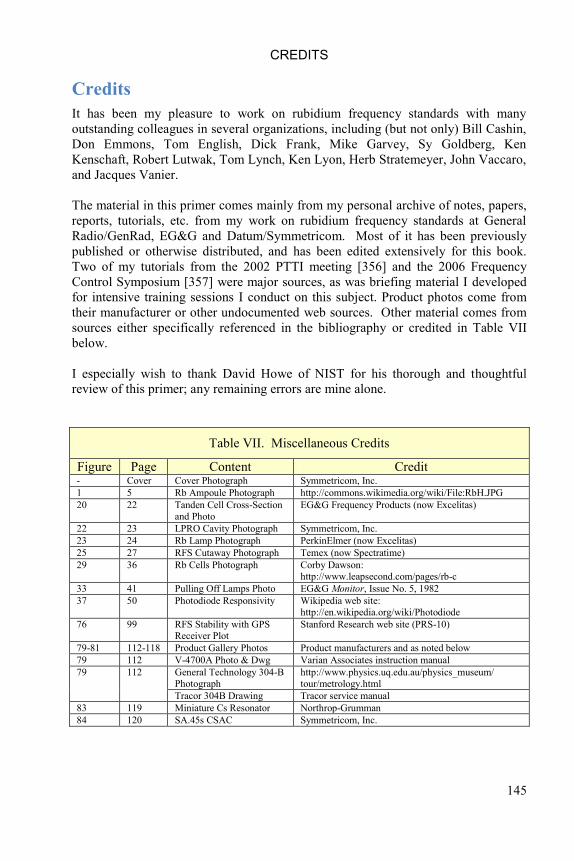
CREDITS
145
Credits
It has been my pleasure to work on rubidium frequency standards with many
outstanding colleagues in several organizations, including (but not only) Bill Cashin,
Don Emmons, Tom English, Dick Frank, Mike Garvey, Sy Goldberg, Ken
Kenschaft, Robert Lutwak, Tom Lynch, Ken Lyon, Herb Stratemeyer, John Vaccaro,
and Jacques Vanier.
The material in this primer comes mainly from my personal archive of notes, papers,
reports, tutorials, etc. from my work on rubidium frequency standards at General
Radio/GenRad, EG&G and Datum/Symmetricom. Most of it has been previously
published or otherwise distributed, and has been edited extensively for this book.
Two of my tutorials from the 2002 PTTI meeting [356] and the 2006 Frequency
Control Symposium [357] were major sources, as was briefing material I developed
for intensive training sessions I conduct on this subject. Product photos come from
their manufacturer or other undocumented web sources. Other material comes from
sources either specifically referenced in the bibliography or credited in Table VII
below.
I especially wish to thank David Howe of NIST for his thorough and thoughtful
review of this primer; any remaining errors are mine alone.
Table VII. Miscellaneous Credits
Figure Page Content Credit - Cover Cover Photograph Symmetricom, Inc.
1 5 Rb Ampoule Photograph http://commons.wikimedia.org/wiki/File:RbH.JPG
20 22 Tanden Cell Cross-Section
and Photo
EG&G Frequency Products (now Excelitas)
22 23 LPRO Cavity Photograph Symmetricom, Inc.
23 24 Rb Lamp Photograph PerkinElmer (now Excelitas)
25 27 RFS Cutaway Photograph Temex (now Spectratime)
29 36 Rb Cells Photograph Corby Dawson:
http://www.leapsecond.com/pages/rb-c
33 41 Pulling Off Lamps Photo EG&G Monitor, Issue No. 5, 1982
37 50 Photodiode Responsivity Wikipedia web site:
http://en.wikipedia.org/wiki/Photodiode
76 99 RFS Stability with GPS
Receiver Plot
Stanford Research web site (PRS-10)
79-81 112-118 Product Gallery Photos Product manufacturers and as noted below
79 112 V-4700A Photo & Dwg Varian Associates instruction manual
79 112 General Technology 304-B
Photograph
http://www.physics.uq.edu.au/physics_museum/
tour/metrology.html
Tracor 304B Drawing Tracor service manual
83 119 Miniature Cs Resonator Northrop-Grumman
84 120 SA.45s CSAC Symmetricom, Inc.


INDEX
147
Index
About the Author ....................................................................................................... iii
Absorption Cells ........................................................................................................35
Advanced Rubidium Clocks ....................................................................................120
Aging .........................................................................................................................91
Analog Control and Monitoring ..............................................................................110
Analog Servo Amplifiers ...........................................................................................53
Applications ...............................................................................................................97
Bibliography ............................................................................................................122
Buffer Gas Considerations .........................................................................................38
Calibration ...............................................................................................................110
C-Field .......................................................................................................................46
Chip Scale Atomic Clocks .......................................................................................119
Copyright Notice ........................................................................................................ ii
Credits ......................................................................................................................145
Crystal Oscillators .....................................................................................................60
Dedication .................................................................................................................. iv
Digital Control and Monitoring ...............................................................................110
Digital Signal Processing ...........................................................................................58
E-Mail ......................................................................................................................... ii
Environmental Sensitivity..........................................................................................84
Fax .............................................................................................................................. ii
Frequency Lock Loops ..............................................................................................55
Frequency Synthesis ..................................................................................................68
Gallery of RFS Products ..........................................................................................111
Glossary and Acronyms ...........................................................................................121
Hamilton Technical Services ...................................................................................... ii
History ........................................................................................................................ 2
Hyperfine Filtration .................................................................................................... 9
Hyperfine Resonances ................................................................................................ 5
Index ........................................................................................................................147
Internal Measurements ...............................................................................................82
Introduction ................................................................................................................ 1
Isotopic Filter Cells ....................................................................................................35
Lamp Life and Calorimetry .......................................................................................28
Laser-Pumped Gas Cell Frequency Standards .........................................................119
Life and Reliability ....................................................................................................95
Light Shift ..................................................................................................................34
Lock Acquisition ................................................................................................. 19, 58
Low Pass or Notch Filtration .....................................................................................54
Magnetic Shielding ....................................................................................................49
Manufacturers ..........................................................................................................111
Mechanical Design ....................................................................................................70
Microwave Cavities ...................................................................................................42

RUBIDIUM FREQUENCY STANDARD PRIMER
148
Optical Pumping ......................................................................................................... 9
Oven Temperature Controllers.................................................................................. 70
Passive Atomic Frequency Standards ....................................................................... 11
Performance .............................................................................................................. 83
Phase Locked Oscillator Multipliers ......................................................................... 68
Phase Noise ............................................................................................................... 77
Photodetectors ........................................................................................................... 50
Physics Package Recipes and Optimizations ............................................................ 23
Power and Thermal Cycling Endurance ................................................................... 95
Preamplifier .............................................................................................................. 51
Pressure Sensitivity ................................................................................................... 86
Pulsed Light .............................................................................................................. 35
Rb Cell Processing .................................................................................................... 40
Rb Discriminator Signal ........................................................................................... 14
Rb Lamp Exciters ..................................................................................................... 29
Rb Lamps .................................................................................................................. 25
Rb Physics Packages ................................................................................................. 13
Rb Resonance Line ................................................................................................... 15
RbXO ...................................................................................................................... 118
RF Chains ................................................................................................................. 61
RFS Internal Operating Adjustments ........................................................................ 81
RFS with GPS Receiver ............................................................................................ 98
Rubidium .................................................................................................................... 5
Rubidium Gas Cell Devices ...................................................................................... 12
Servo Modulation ..................................................................................................... 15
Signal Parameters ..................................................................................................... 78
Software ..................................................................................................................... iii
Specifications ............................................................................................................ 99
Stability ..................................................................................................................... 74
Step Recovery Diode Multipliers .............................................................................. 68
Storage ...................................................................................................................... 96
Synchronous Detection ............................................................................................. 54
Table of Contents ........................................................................................................ v
Table of Figures ......................................................................................................... xi
Temperature Compensation ...................................................................................... 85
Terminology................................................................................................................ 2
Testing .................................................................................................................... 100
The Kenschaft Model ................................................................................................ 19
Thermal Design ......................................................................................................... 72
Vibration Sensitivity ................................................................................................. 87
Warm-up ................................................................................................................... 95
Web ............................................................................................................................. ii

NOTES
149