wittener diskussionspapiere - willkommen am institut für ... · comparable in their risk profile....

Fakultät fürWirtschaftswissenschaft

WittenerDiskussionspapiere

Valuation with Risk-Neutral Probabili-ties: Attempts to Quantify Q

Frank Richter

Christian Timmreck

Heft Nr. 108

Oktober 2002

III

Content

Abstract................................................................................................ V

1 Introduction......................................................................................... 1

2 Risk-adjusted discount rates ................................................................. 2

2.1 Interpretation of common practice.................................................... 2

2.2 Constant discount rate and constant risk premium ............................. 3

2.3 Using the CAPM to determine the risk premium ................................ 3

3 Certainty equivalents, risk-adjusted probabilities, and risk-adjusted

growth rates ......................................................................................... 6

3.1 Outline of the risk-neutral valuation approach .................................... 6

3.2 Simplification of the time-state space: Binomial model ...................... 7

3.3 Risk-adjusted growth rates ............................................................. 11

4 Relationship between the two approaches............................................ 11

4.1 Model-based betas and risk premiums ............................................ 11

4.2 Estimating the market risk premium................................................. 14

4.3 How to estimate q? ........................................................................ 14

4.3.1 Logical boundaries for q........................................................ 15

4.3.2 Using an exogenous estimate for the expected market rate

of return................................................................................ 16

4.3.3 Exogenous estimate for the market rate of return and its

volatility ................................................................................ 18

4.3.4 Using an exogenous estimate for risk premium and current

betas ..................................................................................... 19

4.3.5 Heuristic approach................................................................. 20

IV

5 Example for practical application......................................................... 21

6 Conclusion......................................................................................... 24

Appendix .............................................................................................. 25

References ............................................................................................ 28

V

Abstract

An important and complex question in corporate finance is how to value

uncertain cash-flow streams. Common practice is to discount expected

cash flows with a constant risk-adjusted discount rate. The risk-adjusted

discount rate approach is the basis for discounted cash flow approaches

applied in practice for capital budgeting purposes or for the valuation of

companies. The capital asset pricing model is usually used to determine the

discount rate. This model has, however, theoretical and empirical short-

comings, as, for example, the expected rate of return of the market portfolio

and thereby the expected market risk premium is not observable. An alter-

native approach is applied in the field of option pricing theory: The risk

neutral valuation approach does not require an assumption on the risk pre-

mium. Instead, the analyst needs to quantify the risk-neutral probability.

The aim of this paper is to show the relation between the two approaches

and to find estimates for the risk-neutral probability by using logical argu-

ments and empirical data of the 30 German DAX companies. We illustrate

the risk-neutral valuation approach on the basis of an example that we de-

veloped from publicly available valuation documentation of a recent merger

in Germany.

Keywords: Risk-neutral Probability, Risk Premium, Cost of Capital, Dis-

counted Cash Flow, Certainty Equivalent Approach

JEL-class.: G 32, G12

1 Introduction

An important and complex question in corporate finance is how to value

uncertain future cash-flow streams. Common practice is to discount ex-

pected cash flows with a constant risk-adjusted discount rate. The concept

of risk-adjusted discount rates (RADR) is the basis for common discounted

cash flow (DCF) approaches applied in practice for capital budgeting pur-

poses or for the valuation of companies. The capital asset pricing model

(CAPM) is usually used to determine the RADR. This model has well-

known theoretical and empirical shortcomings, as, for example, the ex-

pected rate of return of the market portfolio and thereby the expected mar-

ket risk premium is not observable. Instead, historical estimates are used to

specify key parameters for the CAPM. This, however, is inconsistent, be-

cause future cash flows are valued with RADR based on historical data. An

alternative approach is applied in the field of option pricing theory: The risk

neutral valuation (RNV) approach does not require an explicit assumption

on the risk premium. Instead, the analyst needs to quantify the risk-neutral

probability. Risk-neutral probabilities are used to transform uncertain cash

flows into their certainty equivalents. These certainty equivalents can be

discounted at the risk-free interest rate.

The aim of this paper is to show the relation between the two approaches

and to find estimates for the risk-neutral probability by using logical argu-

ments and empirical data of the 30 German DAX companies. We illustrate

the risk-neutral valuation approach on the basis of an example that we de-

veloped from publicly available valuation documentation of a recent merger

in Germany. Chapter 2 summarises the RADR approach and points out

key issues regarding the application of the CAPM. The RNV approach is

presented in chapter 3. We will use a binomial model as simplified structure

for the cash-flow stream and develop a valuation formula, which is consis-

tent with but not dependent on the CAPM. After the two valuation ap-

proaches have been presented we discuss their relationships in chapter 4.

Richter/Timmreck: Valuation with Risk-Neutral Probabilities

2

Model-based betas and risk premiums are derived from the RNV approach

for different assumptions on the risk-neutral probabilities. We will derive

the logical limits for risk-adjusted probabilities. In addition we use empirical

data to narrow the range. Based on this analysis we suggest a heuristic ap-

proach to quantify risk-neutral probabilities. This approach is applied to a

case based on real data (chapter 5). Chapter 6 closes with a brief summary.

2 Risk-adjusted discount rates

2.1 Interpretation of common practice

The common approach to value uncertain cash-flow streams e.g. for capital

budgeting purposes is to discount unconditional expected cash flows,

][ tiP C~

E , with a risk-adjusted discount rate called the cost of capital of the

asset i, ir , which produces the cash-flow stream:1

(1) ∑ =−+][= T

1tt

itiPi0 )r1( C~

EV

The subscript P of the expectation operator indicates that the subjective

probability p is used to formulate expected cash flows.2 The risk aversion

of investors is taken into account by using the cost of capital as a discount

rate, which typically exceed the risk-free interest rate by a risk premium.3

This approach is an application of the concept of risk-adjusted discount

rates (RADR).

1 Our interpretation of common practice is based on standard text books in finance such as

Brealey, R.A./ Myers, S.C. (1996) and management literature, e.g., Copeland, T.E./Koller, T./ Murrin, J. (2000).

2 Expectations without reference to a specific filtration indicate unconditional expectations.3 For simplicity purposes we assume only positive risk premiums and therefore risk-averse


3

2.2 Constant discount rate and constant risk premium

We assume that the risk-free rate fr is certain and not time dependent, al-

though this is only for simplicity purposes. More important is the assump-

tion that is found in the majority of practical applications, i.e., the assump-

tion that the risk premium iπ is constant through time:

(2) ifi rr π+=

It shall be pointed out that the use of a constant risk premium is warranted

only under specific conditions. Sufficient conditions for the use of constant

risk premiums have been described as “simplified discounting rules”. If, for

example, the uncertain cash-flow stream follows a martingale with constant

growth, the application of a constant risk premium to value this stream is

sensible.4

In practice, it is often not possible to verify whether the conditions for sim-

plified discounting rules are met, given that the cash-flow streams taken

from business plans do not unveil the assumptions on the stochastic prop-

erties of that stream. Thus, the application of constant risk premiums is

more a heuristic approach than anything else.

2.3 Using the CAPM to determine the risk premium

The Capital Asset Pricing Model (CAPM) is a positive theory of expected

rates of return, which often serves as a basis to estimate the risk premium.

In order to do so the analyst needs to quantify his or her expectation re-

garding the market risk premium, i.e., the difference between the expected

rate of return of the market portfolio, ][ mP r~E , relative to the risk-free inter-

investor.


4

est rate. In addition, the beta is needed that relates the rate of return of the

asset i to the rate of return of the market portfolio:5

(3) ]−[β=π fmPii rr~E

][][

=βm

mii r~var

r~,r~cov

The application of the CAPM is conceptually easy, however, empirical is-

sues are evident: What is a reliable estimate for the expected market rate of

return? Where does the beta come from, if the rates of returns of the asset i

are not observable?

The heuristic “solution” is to use estimators based on historical data and

comparable assets that are traded in a market. For example, the historic

market risk premium often is estimated in the range between 3 % and 7 %6

per annum. These estimates are based on time series of historic rates of

return of a diversified stock market index versus interest rates of govern-

ment bonds. Betas are taken from traded assets, which are assumed to be

comparable in their risk profile. Table 1 shows the cost of capital for the

DAX 30 companies, using a risk premium of 5 %,7 a risk-free rate of 5 %

and betas from Bloomberg. Raw betas are only based on historical data, in

contrast to adjusted betas which are weighted averages of the raw beta (2/3)

and the market beta (1/3). Based on this information, the average cost of

capital is 10 %.

4 See Richter, F. (2001) and (2002).5 See e.g., Weston, J.F./ Copeland, T.E. (1988) p. 195 - 198, or the original article by

Sharpe, W. (1964) p. 425 - 442.6 Claus, J./ Thomas, J. (2001), Fama, E./ French, K.R. (2000) or Cornell, B. (1999).7 Stehle, R (1999) estimates, Morawietz, M., (1994), Bimberg, L. (1991), Uhlir, H./ Stei-

ner, P. (1991), and other studies.


5

Table 1 Betas and Cost of Capital for DAX members

Company raw Beta CoC on adjusted CoC onraw Beta Beta adj. Beta

Adidas 0.62 8.1% 0.75 8.7%Allianz 0.91 9.5% 0.94 9.7%BASF 0.82 9.1% 0.88 9.4%Bayer 0.76 8.8% 0.84 9.2%HypoVereinsbank 0.68 8.4% 0.78 8.9%BMW 0.87 9.3% 0.91 9.6%Commerzbank 0.87 9.3% 0.91 9.6%DaimlerChrysler 0.91 9.5% 0.94 9.7%Deutsche Bank 1.14 10.7% 1.09 10.5%Degussa 0.70 8.5% 0.80 9.0%Lufthansa 0.99 10.0% 1.00 10.0%Deutsche Post n.a. n.a. n.a. n.a.Telekom 1.23 11.2% 1.15 10.8%Eon 0.31 6.5% 0.53 7.7%Epcos 1.51 12.5% 1.34 11.7%Fresenius 0.50 7.5% 0.66 8.3%Henkel 0.16 5.8% 0.44 7.2%Infineon n.a. n.a. n.a. n.a.Linde 0.52 7.6% 0.68 8.4%MAN 0.62 8.1% 0.75 8.7%Metro 0.59 7.9% 0.72 8.6%MLP 1.00 10.0% 1.00 10.0%Münchner Rück 0.79 9.0% 0.86 9.3%Preussag 1.02 10.1% 1.01 10.1%RWE 0.44 7.2% 0.63 8.1%SAP 1.62 13.1% 1.42 12.1%Schering 0.37 6.8% 0.58 7.9%Siemens 1.50 12.5% 1.33 11.7%ThyssenKrupp 0.79 8.9% 0.86 9.3%Volkswagen 0.81 9.0% 0.87 9.4%

Market Portfolio 1.00 10.0% 1.00 10.0%


6

3 Certainty equivalents, risk-adjusted probabilities, and risk-

adjusted growth rates

Even if the empirical issues of the RADR in combination with CAPM are

resolved to the satisfaction of the analyst, one issue remains: It is not con-

sistent to value future cash-flow streams with cost of capital based on his-

toric risk premiums. The expected future risk premium should be employed

instead. Therefore, we search for an approach that does not need an ex-

ogenous assumption on the market risk premium. In addition, the approach

should allow for a time-varying risk premium.

3.1 Outline of the risk-neutral valuation approach

The certainty equivalent approach works as follows: Instead of discounting

unconditional cash-flow expectations with a risk-adjusted discount rate,

certainty equivalent cash flows are discounted at the risk-free interest rate:8

(4) ∑ =−+]|[= T

1tt

f0tiQi0 )r1( FC~

EV

The risk aversion of investors is taken into account by reducing the ex-

pected cash flow under P. This is done on the basis of an equivalent prob-

ability measure Q, which creates conditional certainty equivalents as indi-

cated by the filtration F. A risk-averse investor relates expected cash flows

to the certainty equivalent as follows: ][<]|[ tiP0tiQ C~

EFC~

E . In the option

pricing literature, this approach is called “risk-neutral valuation” (RNV). In

a first step the expected cash flows are reduced via the risk-neutralised

probabilities. In a second step, this modified cash-flow expectation is val-

ued as if investors would be risk neutral, i.e., by discounting with the risk-

free rate.

8 See e.g. Duffie, D. (1988) for more background on this approach.


7

3.2 Simplification of the time-state space: Binomial model

The application of the RADR approach requires simplifications, e.g., when

determining the risk premium. The same holds true for the RNV approach,

however, the heuristic simplification follows a different route. A simplified

stochastic model for the uncertain cash-flow stream is assumed, which

makes the time-state space tractable. The application of the binomial model

is an example for this. Within this model future cash flows can either move

up by the factor tiu or shrink by tid as shown in exhibit 1, i.e.,

{ }tii,ttii,ti,1t dC~

;uC~

C~ ∈+ , with titi ud0 ≤< . Both probability measures P

and Q can be applied to the cash-flow process, being it to determine the

subjective (unconditional) expectations or certainty equivalents.

The binomial model is a heuristic because the true stochastic model of the

future cash-flow stream often is not known. Assuming that this is an ac-

ceptable simplification, the next question is how to estimate the parameters

of the model. These parameters can be taken from the business plan for the

asset to be valued. The analyst shall be able to articulate the expectations of

the period-by-period growth rates 1C~

E/C~

Eg i,tPi,1tPti −][][= + . Fixing p

and assuming a recombining binomial model the up and down factors are

determined:9

(5)p

p1

p2

g1

p2

g1u

2titi

ti−

−

++

+=

titi u

1d =

9 Formulas for non-recombining trees are shown in the appendix.


8

With that we have a binomial model that is consistent with the expected

growth rates of the business plan: tititi d)p1(pug1 −+=+ .

Exhibit 1 Binomial Model

Tables 2 and 3 contain the growth factors derived from the I/B/E/S data-

base for the DAX 30 companies (p = ½). We use two sets of data, based on

the growth rates of expected dividends per share, DPS, and the growth

rates of expected earnings per share, EPS. These are proxies for the

growth rates of expected cash flows to shareholders, both of which are not

perfect, given that the first lacks share buy-backs and capital increase and

the second often is not fully distributed to shareholders. However, better

estimates are not available.10

10 The following abbreviations are used: na = not available, neg = negative growth rate, caa =

change of accidental, nc = not considered. In all of these cases the derivation of the growthfactor u is not possible or not sensible with our approach. Therefore we left the corre-sponding companies out. Furthermore companies with negative growth rates have negativecorrelation with a market which has positive growth rates, and we assume positive corre-

Binomial Model: In each time-step only two possible states

Calculation of (conditional) expected cash flows:

0C

i10 uC ⋅

i10 dC ⋅

i2i10 ddC ⋅⋅

i2i10 udC ⋅⋅

i2i10 uuC ⋅⋅

p

p1−

0t = 1t = 2t =

i10i1001P dC)p1(uCp]FC~

[E ⋅⋅−+⋅⋅=

i2i10i2i1012P udC)p1(uuCp]FC~

[E ⋅⋅⋅−+⋅⋅⋅= or:

i2i10i2i1012P ddC)p1(udCp]FC~

[E ⋅⋅⋅−+⋅⋅⋅=


9

Table 2 DPS growth rates, and related growth factors

lation in general.

Comapny Growth rate up- down- Growth rate up- down- Growth rate up- down-2002 factor factor 2003 factor factor 2004 factor factor

Adidas 5.8% 1.404 0.712 12.9% 1.652 0.605 -3.0% neg. neg.Allianz 22.4% 1.931 0.518 14.2% 1.693 0.591 n.a. n.a. n.a.BASF 4.8% 1.363 0.734 4.3% 1.340 0.746 -6.9% neg. neg.Bayer 8.9% 1.520 0.658 11.4% 1.606 0.623 11.9% 1.621 0.617HypoVereinsbank 9.9% 1.555 0.643 13.7% 1.677 0.596 -15.8% neg. neg.BMW 5.7% 1.400 0.714 10.2% 1.565 0.639 24.0% 1.974 0.507Commerzbank 14.1% 1.691 0.591 7.2% 1.459 0.685 -39.4% neg. neg.DaimlerChrysler 10.6% 1.579 0.633 13.9% 1.683 0.594 n.a. n.a. n.a.Deutsche Bank 9.2% 1.532 0.653 14.2% 1.693 0.591 -3.4% neg. neg.Degussa 6.1% 1.416 0.706 8.9% 1.520 0.658 11.5% 1.608 0.622Lufthansa 22.4% 1.929 0.518 13.1% 1.661 0.602 10.8% 1.585 0.631Deutsche Post 3.5% 1.300 0.769 5.1% 1.375 0.727 n.a. n.a. n.a.Telekom -1.7% neg. neg. 3.6% 1.305 0.766 2.9% 1.270 0.788Eon 8.4% 1.501 0.666 5.1% 1.376 0.727 6.6% 1.435 0.697Epcos 8.2% 1.496 0.668 2.1% 1.227 0.815 58.1% 2.806 0.356Fresenius 12.6% 1.644 0.608 5.3% 1.384 0.723 n.a. n.a. n.a.Henkel 11.7% 1.615 0.619 9.2% 1.531 0.653 15.9% 1.744 0.573Infineon n.a. n.a. n.a. n.a. n.a. n.a. n.a. n.a. n.a.Linde 6.0% 1.413 0.708 3.0% 1.276 0.784 13.3% 1.665 0.601MAN 1.1% 1.160 0.862 11.9% 1.622 0.617 n.a. n.a. n.a.Metro 2.9% 1.269 0.788 3.9% 1.320 0.757 6.4% 1.428 0.700MLP 29.3% 2.112 0.473 50.8% 2.636 0.379 27.4% 2.064 0.484Münchner Rück 15.7% 1.740 0.575 9.4% 1.538 0.650 29.4% 2.115 0.473Preussag 6.5% 1.431 0.699 10.4% 1.572 0.636 6.7% 1.438 0.696RWE 10.0% 1.560 0.641 12.7% 1.647 0.607 21.5% 1.906 0.525SAP 33.9% 2.229 0.449 22.6% 1.934 0.517 40.4% 2.389 0.419Schering 16.4% 1.758 0.569 10.8% 1.584 0.631 23.9% 1.972 0.507Siemens 5.8% 1.402 0.713 15.6% 1.736 0.576 17.0% 1.778 0.562ThyssenKrupp -1.0% neg. neg. 12.7% 1.648 0.607 -2.0% neg. neg.Volkswagen 5.1% 1.375 0.727 5.3% 1.382 0.723 38.2% 2.335 0.428


10

Table 3 EPS growth rates, and related growth factors

Comapny Growth rate up- down- Growth rate up- down- Growth rate up- down-2002 factor factor 2003 factor factor 2004 factor factor

Adidas 12.7% 1.648 0.607 17.0% 1.777 0.563 -19.2% neg. neg.Allianz 49.1% 2.597 0.385 11.8% 1.618 0.618 n.a. n.a. n.a.BASF 35.1% 2.259 0.443 25.2% 2.004 0.499 10.1% 1.563 0.640Bayer 23.8% 1.968 0.508 27.9% 2.077 0.481 9.8% 1.552 0.644HypoVereinsbank 25.2% 2.006 0.498 35.8% 2.277 0.439 21.5% 1.904 0.525BMW 5.4% 1.388 0.721 12.8% 1.651 0.606 0.6% 1.114 0.898Commerzbank 74.3% 3.170 0.315 26.7% 2.044 0.489 n.a. n.a. n.a.DaimlerChrysler 190.5% 5.633 0.178 58.0% 2.802 0.357 38.9% 2.354 0.425Deutsche Bank 9.1% 1.526 0.655 15.2% 1.724 0.580 -0.3% neg. neg.Degussa 0.3% 1.076 0.929 26.4% 2.037 0.491 8.5% 1.506 0.664Lufthansa 174.3% 5.298 0.189 50.2% 2.622 0.381 71.3% 3.105 0.322Deutsche Post -3.4% neg. neg. 0.8% 1.134 0.882 n.a. n.a. n.a.Telekom -12.5% neg. neg. caa caa caa 66.2% 2.990 0.334Eon 20.2% 1.869 0.535 13.1% 1.660 0.603 -0.3% neg. neg.Epcos -7.8% neg. neg. 47.6% 2.562 0.390 62.2% 2.899 0.345Fresenius 21.3% 1.898 0.527 15.9% 1.744 0.573 20.6% 1.880 0.532Henkel 9.1% 1.528 0.655 9.8% 1.552 0.644 3.7% 1.309 0.764Infineon 21.6% 1.907 0.524 caa caa caa -73.8% neg. neg.Linde 14.5% 1.703 0.587 15.4% 1.731 0.578 21.9% 1.917 0.522MAN 14.3% 1.696 0.590 22.5% 1.932 0.518 0.1% 1.054 0.949Metro 13.5% 1.671 0.598 15.2% 1.723 0.581 2.3% 1.239 0.807MLP 33.1% 2.209 0.453 41.1% 2.406 0.416 -3.3% neg. neg.Münchner Rück 58.1% 2.804 0.357 18.5% 1.821 0.549 24.4% 1.985 0.504Preussag 8.5% 1.506 0.664 5.3% 1.382 0.724 36.7% 2.300 0.435RWE 19.1% 1.839 0.544 15.2% 1.723 0.580 22.9% 1.945 0.514SAP 36.3% 2.289 0.437 39.5% 2.367 0.422 27.0% 2.054 0.487Schering 14.4% 1.700 0.588 15.1% 1.721 0.581 16.0% 1.748 0.572Siemens 75.4% 3.196 0.313 80.2% 3.301 0.303 24.5% 1.988 0.503ThyssenKrupp 11.7% 1.614 0.619 28.1% 2.081 0.480 32.9% 2.205 0.454Volkswagen -0.4% neg. neg. 5.8% 1.404 0.712 36.5% 2.295 0.436


11

3.3 Risk-adjusted growth rates

Next, we apply the risk-neutral probability q instead of p to determine the

risk-adjusted growth rate:

(6) titi*ti d)q1(qug1 −+=+

The risk-adjusted growth rates now can be used to derive the certainty

equivalents needed to apply the RNV approach as indicated by (4):

(7) ∏ = +=]|[ t1j

*jii00tiQ )g1(CFC

~E

Notice that (1) is bound to the case of constant growth rates while (7) is

not. To apply (1) the empirical issue of determining π has to be resolved.

(7) requires quantification of q instead. Before we come to that the relation-

ships between (1) and (7) shall be made more transparent.

4 Relationship between the two approaches

4.1 Model-based betas and risk premiums

From a conceptual view both approaches are equivalent if the RADR is ap-

plied with consistent risk premiums. Under the assumption of the binomial

model as described in the previous section, the cost of capital and thereby

the risk premium is given by:11

(8) tifftiti r1)r1(xr π+=−+=

11 See Richter, F. (2002), p. 138.


12

*ti

titi

g1

g1x

++

=

⇒ )r1)(1x( ftiti +−=π

To determine the risk-adjusted discount rate the risk-free rate is grossed-up

by a factor of tix , which depends on the growth rate of the expected cash

flow relative to the growth rate of the certainty equivalent of the cash flow.

This relation is supposed to hold for any asset, a portfolio of assets and for

the market as a whole, i.e. for i = m. As shown in the appendix this imme-

diately provides us with an interpretation of beta in the sense of the CAPM:

(9)1x

1x

tm

titi −

−=β

The RADR approach and the RNV approach yield the same result if the

discount rate according to (8) or (9) is used.

The next two exhibits illustrate the relation between growth and expected

rate of return, and beta, respectively. The graphs are plotted for various

assumptions on q. With q = p = ½ we expected rates of return equal to the

risk-free rate of return. Investors who do not differentiate between p and q

are risk-neutral. Therefore, there is no risk premium, although beta is posi-

tive and increasing with growth. The other extreme, q = 0, characterises

maximum risk aversion, given that q is the risk-adjusted probability for up-

ward movements. With q = 0, only downward movements are taken into

account. This implies maximum betas and maximum expected rates of re-

turn.12

12 We assume that the correlation between the cash flows from asset i and the cash flows

from the alternative investment, i.e. from the market, is positive and perfect. Therefore ourresults will be maximum risk premiums.


13

Expected rate of return (q = 0, 0.1, 0.2, 0.3, 0.4, 0.5; rf = 5 %)

0%

10%

20%

30%

40%

50%

60%

70%

80%

90%

100%

0% 20% 40% 60% 80% 100%

Growth gm or gi

Exp

ecte

d r m

or

r i

Exhibit 2 Expected Rate of Return as a function of growth and q

Beta (q = 0, 0.1, 0.2, 0.3, 0.4, 0.5; rf = 5 %; gm = 10 %)

0.0

0.5

1.0

1.5

2.0

2.5

3.0

3.5

4.0

0% 20% 40% 60% 80% 100%

Growth gi

Bet

a

Exhibit 3 Beta as a function of growth and q


14

4.2 Estimating the market risk premium

We can use the model to estimate the expected market risk premium. Here

is our idea: We plan to derive a forward-looking risk premium of the market

portfolio from the weighted average of the risk premiums of all assets,

which constitute this portfolio. We will again use analyst expectations as

shown in tables 2 and 3. The expected growth rate for the market portfolio

and its corresponding risk-adjusted growth rate are given by (10) and (11):

(10) 1C~

E

C~

Eg

n1i i,1tP

n1i tiP

tm −][

][=

∑∑

= −

= with ∏ = +=][ t1j tii0tiP )g1(CC

~E

(11) 1FC

~E

FC~

Eg

0n

1i i,1tQ

n1i 0tiQ*

tm −]|[

]|[=

∑∑

= −

= with ∏ = +=]|[ t1j

*jii00tiQ )g1(CFC

~E

Given these two growth rates we can employ (8) to determine tmx and

thereby tmπ .

4.3 How to estimate q?

The final parameter that we need is q. We take four approaches: First, we

look at the range of attainable values for q, which are given by its logical

limits. Then, we use an increasing set of empirical data to narrow the

bandwidth of potential values for q. The second approach is based on ex-

ogenous estimates for the expected market rates of return. Third, we in-

clude an estimate for the volatility of the market rate of return. Fourth, we

use the exogenous estimate for the expected market rate of return in combi-

nation with observed betas.


15

4.3.1 Logical boundaries for q

Our model still lacks quantification of q. Here we are at the main purpose

of this paper. Without further specification (other than the binomial model)

we can define the interval of attainable values for q: q has to exceed zero,

otherwise Q would not be an equivalent probability measure to P, given that

we assume p > 0. Furthermore, q may not exceed p in order to transform

the expectation under P into certainty equivalents.13 For the purpose of our

analysis the boundaries for q are as follows:

(12) 5.0pq0 =≤<

With this boundaries we can determine the maximum and the minimum risk

premium and thereby the minimum and the maximum value of cash-flow

streams. This interval of attainable values is bound to the assumptions of

the binomial model and the assumption of arbitrage-free markets only. No

historic data is used at all. However, the bandwidth of attainable risk premi-

ums is very broad and sensitive to q.

Table 4 Expected Market Rate of Return for different q based on DPS

13 Again we assume positive correlation between the asset and the market.

q 2002 2003 2004

0 63.9% 78.0% 60.8%0.1 47.4% 56.3% 45.4%0.2 33.9% 39.3% 32.6%0.3 22.6% 25.6% 21.9%0.4 13.1% 14.4% 12.8%0.5 5.0% 5.0% 5.0%

Expected Market Rate of Return (DPS)


16

Table 5 Expected Market Rate of return for different q based on EPS

4.3.2 Using an exogenous estimate for the expected market rate of return

Assume, the expected risk premium for the market portfolio would be

given, e.g., with [ ]%7%,3ˆ ∈π . The risk-free interest rate can be derived

from observable data, say %5rf = . With that we have an estimate for the

expected rate of return, which in turn can be used to derive q:

(13) 1)r1(g1

g1r̂ f*

tm

tmm −+

++

=

1r̂1

r1)g1(g

m

ftm

*tm −

++

+=⇒

tmtm

tmm

ftm

tmtm

tm*tm

t du

dr̂1

r1)g1(

du

dg1q

−

−++

+=

−−+

=⇒

q 2002 2003 2004

0 202.2% 209.9% 126.9%0.1 119.7% 122.9% 84.2%0.2 72.6% 74.1% 55.0%0.3 42.1% 42.8% 33.7%0.4 20.8% 21.0% 17.6%0.5 5.0% 5.0% 5.0%

Expected Market Rate of Return (EPS)


17

The advantage of this approach is that we get a point estimate for the risk-

neutral probability. However, we need an estimate for the expected rate of

return of the market portfolio. As pointed out earlier, it is not consistent to

use historic data to produce such an estimate. Notice, that if a constant risk

premium is assumed, the risk-neutral probabilities become time-dependent.

Nevertheless, based on a fairly broad range of market risk premiums, the

range of attainable q values is between 0.410 and 0.479.

Table 6 Possible q-values based on exogenous estimates for the marketrisk premium (on DPS)

Table 7 Possible q-values based on exogenous estimates for the marketrisk premium (on EPS)

RiskPremium 2002 2003 2004

3% 0.461 0.466 0.4604% 0.449 0.455 0.4475% 0.437 0.445 0.4356% 0.425 0.434 0.4227% 0.413 0.424 0.410

Implied value for q (DPS)

RiskPremium 2002 2003 2004

3% 0.479 0.479 0.4744% 0.472 0.472 0.4665% 0.465 0.466 0.4586% 0.459 0.459 0.4507% 0.452 0.453 0.442

Implied value for q (EPS)


18

4.3.3 Exogenous estimate for the market rate of return and its volatility

Assume we would have a reliable estimate for the rate of return of the mar-

ket portfolio (with %5rf = and [ ]%7%,3ˆ ∈π ). In addition, the volatility of

the market rate of return shall be given, e.g., { }3.0,275.0,25.0ˆ m ∈σ .14 If

these parameters are supposed to be constant through time, we can derive

the underlying value for q:

(14) f

!

mm,1ttmm,1tt1ttmQ r)ˆr)(q1()ˆr(qFr~E =σ−−+σ+=]|[ −−−

2

1q tm

tφ−

=⇒

with m

fm,1ttm ˆ

rr

σ−

=φ − (also known as Sharpe-ratio)

The expected market rate of return under the risk-adjusted probability q has

to equal the risk free rate. Under the assumed structure for the market rate

of return q could be derived from the expected risk premium in connection

with the volatility of the market rate of return. Formula (14) rests on the ab-

sence of arbitrage. It is clear that we have the implicit assumptions of a per-

fect correlation between the rates of return of the security i and the rates of

return on the market portfolio.

14 See Bimberg, L. (1991).


19

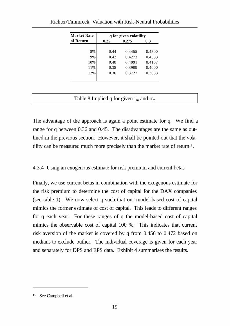
Table 8 Implied q for given rm and σm

The advantage of the approach is again a point estimate for q. We find a

range for q between 0.36 and 0.45. The disadvantages are the same as out-

lined in the previous section. However, it shall be pointed out that the vola-

tility can be measured much more precisely than the market rate of return15.

4.3.4 Using an exogenous estimate for risk premium and current betas

Finally, we use current betas in combination with the exogenous estimate for

the risk premium to determine the cost of capital for the DAX companies

(see table 1). We now select q such that our model-based cost of capital

mimics the former estimate of cost of capital. This leads to different ranges

for q each year. For these ranges of q the model-based cost of capital

mimics the observable cost of capital 100 %. This indicates that current

risk aversion of the market is covered by q from 0.456 to 0.472 based on

medians to exclude outlier. The individual coverage is given for each year

and separately for DPS and EPS data. Exhibit 4 summarises the results.

15 See Campbell et al.

0.25 0.275 0.3

8% 0.44 0.4455 0.45009% 0.42 0.4273 0.4333

10% 0.40 0.4091 0.416711% 0.38 0.3909 0.400012% 0.36 0.3727 0.3833

Market Rate of Return

q for given volatility


20

Exhibit 4 Necessary q to cover the observed CoC

4.3.5 Heuristic approach

Now we have ranges for the value of q based on its logical boundaries, and

we have some guidance based on empirical data (which is, admittedly,

based on historic information). If we combine all results it appears reason-

able to us to assume a range for q between 0.36 and 0.48. This range lies

within the logical boundaries, fits with the implied values for frequently used

risk premiums, and covers the majority of observable cost of capital esti-

mates for the DAX companies. As our aim is to estimate a company value

eventually it is more appropriate to take the average of the range and use

0.42 as value for q. Therefore we suggest using this as a heuristic to value

uncertain cash-flow streams. We think that this procedure is more robust

than the RADR in combination with the CAPM, given that (i) we do not

have to rely on its assumptions, (ii) we allow for time-varying risk premi-

ums, (iii) we are using forward looking data to the extend possible. The

application of this heuristic is illustrated in the next chapter.

Implied Q for observed Beta

0.2

0.25

0.3

0.35

0.4

0.45

0.5

EPS 2002 EPS 2003 EPS 2004 DPS 2002 DPS 2003 DPS 2004


21

5 Example for practical application

After the merger of two diversified companies in Germany the CEO decided

also to merge the subsidiaries D and S in the area of chemical specialities to

realise synergies and achieving a leading position in this market. As both

subsidiaries have been quoted it is necessary with regard to German law to

publish a merger report with detailed information about the share exchange

ratios. This exchange ratio is determined on the basis of company valuation

with discounted cash flow methods. For the following case study we used

these publicly available data, i.e. the planned earnings before interest and tax

(EBIT) for the next three years and an assumed long term growth rate of 1

%. Furthermore we considered an average corporate tax rate of 38.5 %

according to German tax code. Finally we have no indication for a negative

correlation between growth rate and market rate of return. Therefore we

could apply our heuristic approach on the figures of company D and S as

follows:

Table 9 Application of the heuristic on company D

Company D t=0 1 2 3 4 +EBIT 680.6 844.9 1,001.4 1,224.5Corporate Tax 262.0 325.3 385.5 471.4Unlevered Cash Flow 418.6 519.6 615.9 753.1

Growth Rate of Cash Flow 24.14% 18.52% 22.28% 1.00%Probability (P) 0.5 0.5 0.5 0.5up 1.98 1.82 1.93 1.15down 0.51 0.55 0.52 0.87

Risk adjusted Probability (Q) 0.42 0.42 0.42 0.42Risk adjusted Growth Rate 12.37% 8.34% 11.02% -1.27%Certainty Equivalent of Cash Flow 470.4 563.0 683.7 11,861.3Discount Factor 0.95 0.91 0.86 0.86NPV of Cash Flow 11,795.5 448.0 510.6 590.6 10,246.3Implied Cost of Capital 16.00% 9.82% 8.44% 8.42%


22

Table 10 Application of the heuristic on company S

Under the RNV theorem with the heuristic of q = 0.42 the value for com-

pany D is about € 11,795.5 million and for company S € 5,135.2 million.

This leads to an share exchange ratio of 1 : 2.3 in favour for company D.

The results of a detailed valuation for both companies are represented as

value bandwidths in exhibit 6 and 7.

Company S t=0 1 2 3 4 +EBIT 376.7 420.4 472.5 526.1Corporate Tax 145.0 161.9 181.9 202.5Unlevered Cash Flow 231.7 258.5 290.6 323.6

Growth Rate of Cash Flow 11.60% 12.39% 11.34% 1.00%Probability (P) 0.5 0.5 0.5 0.5up 1.61 1.64 1.60 1.15down 0.62 0.61 0.62 0.87

Risk adjusted Probability (Q) 0.42 0.42 0.42 0.42Risk adjusted Growth Rate 3.67% 4.18% 3.51% -1.27%Certainty Equivalent of Cash Flow 240.2 269.4 300.8 5,096.2Discount Factor 0.95 0.91 0.86 0.86NPV of Cash Flow 5,135.2 228.7 244.3 259.8 4,402.3Implied Cost of Capital 13.03% 9.06% 7.58% 8.42%


23

Exhibit 5 Bandwidth for company Ds value

Exhibit 6 Bandwidth for company Ss value

Value Range for company D

0 5,000 10,000 15,000 20,000

Heuristic

Exog. MRR & Beta

Exog. MRR & Vola

Exog. MRR

Logical Boundaries

X

Value Range for Company S

0 2,000 4,000 6,000 8,000 10,000

Heuristic

Exog. MRR & Beta

Exog. MRR & Vola

Exog. MRR

Logical Boundaries

X


24

6 Conclusion

The commonly used risk-adjusted discount rate approach rests on the

CAPM, assumes constant risk premiums and relies heavily on historical data

to determine the discount rate for future cash flows. The risk-neutral valua-

tion approach overcomes these shortcomings. We think that the risk-neutral

valuation approach is preferable relative to the risk-adjusted discount rate

approach in combination with the CAPM, provided that we have an estimate

for the risk-neutral probability (q), which was the purpose of this paper.

We derived the logical boundaries for q and used empirical data as guidance

to find a range for likely values for q. We think that q lies in the area of 0.36

– 0.48, although more empirical work using a broader set of companies

seems sensible.

A value for q can be used for a heuristic application of the risk-neutral

valuation approach. The value has to be in line with the logical boundaries

of q and should be consistent with cost of capital estimates. Our indication

for this value (0.42) fulfils these requirements for the DAX 30 companies.

The practical application of this heuristic is straightforward, as has been il-

lustrated in our case study.


25

Appendix

(i) Formulas for non-recombining trees

Define g as the expected growth rate and σ as the standard deviation of this

growth rate. In a binomial model we have the following relations:

d)p1(pug1 −+=+

222 )g1d)(p1()g1u(p −−−+−−=σ

From the first definition we get a formula for u:

pd)p1(g1

u−−+

=

Inserting this into the second definition gives us the expression for d:

22

2 )g1d)(p1(g1p

d)p1(g1p −−−+

−−−−+=σ

( ) 22 )g1d)(p1()g1(pd)p1(g1p1

−−−++−−−+⇔

( ) 222

)g1d)(p1(dg1p

)p1(−−−+−+

−⇔

( )22

dg1)p1(p

)p1(−+

−+

−⇔

p1p

)g1(d)g1(2d 222

−σ−+++−⇒

p1p

g1d−

σ−+=⇒

Given g, σ and p, we clearly can derive d. In the case of p = ½ it is simply

one plus growth minus one standard deviation.


26

Finally, we can use this result and substitute d in the formula for u:

p

p1p

)p1()g1)(p1(g1

pd)p1(g1

u−

σ−++−−+=

−−+=

pp1

g1u−σ++=⇔

Again, in the special case of p = ½ we get one plus growth plus one standard

deviation for the upward factor.

In the case of a recombining tree, the variance and the standard deviation of

the growth rate are implicitly defined:

p

p1g1

1p1

pg1d

−σ++

=−

σ−+=

( )2222 1)g1())g1(5.0()g1(5.0 −++α++α+=σ⇒

with p

p1p1

p −−−

=α

For the special case of p = ½ this expression reduces with α = 0 to:

1)g1( 22 −+=σ

Thus, the use of recombining trees replaces the need to specify the standard

deviation of future growth rates by an implicit assumption. In recombining

models, the standard deviation depends on the expected growth rate only.


27

(ii) Derivation of Beta

According to the CAPM we have:

)rr(rr ftmtifti −β+=

ftm

ftiti rr

rr

−−

=β⇒

We use (9) to substitute the expected rate of return for the asset i as well as

for the market rate of return:

1)r1(xr ftiti −+=

1)r1(xr ftmtm −+=

1x

1x

)r1()rf1(x

)r1()rf1(x

r1)rf1(x

r1)rf1(x

tm

ti

ftm

fti

ftm

ftiti −

−=

+−++−+

=−−+−−+

=β⇒

q.e.d.


28

References

Bimberg, L. (1991), Langfristige Renditeberechnungen zur Ermittlung von

Risikoprämien, Frankfurt/ Main.

Brealey, R.A./ Myers, S.C. (1992), Principles of Corporate Finance, New

York.

Campbell, J./ Lo, A./ MacKinlay, C. (1997), The Econometrics of Financial

Markets, Princeton.

Claus, J./ Thomas, J. (2001), Equity premia as low as three percent?, in:

Journal of Finance, Vol. 56, pp. 1629 – 1666.

Copeland, T.E./ Koller, T./ Murrin, J. (2000), Valuation – Measuring and

Managing the Value of Companies, New York.

Duffie, D. (1988), Security Markets, Stochastic Models, San Diego.

Fama, E./ French, K.R. (2000), The Equity Risk Premium, Working Paper

Morawietz, M. (1994), Rentabilität und Risiko deutscher Aktien- und Rente-

nanlagen seit 1870, Wiesbaden.

Richter, F. (2001), Simplified Discounting Rules in Binomial Models, in:

sbr, Vol. 53, pp. 175 – 196.

Richter, F. (2002), Simplified Discounting Rules, Variable Growth, and

Leverage, in: sbr, Vol. 54, pp. 136 – 147.

Sharpe, W.F. (1964), Capital Asset Prices: A Theory of Market Equilibrium

under Conditions of Risk, in: Journal of Finance, Vol. 19, pp. 425 –

442.

Stehle, R. (1999), Renditevergleich von Aktien und festverzinslichen Wert-

papieren auf Bais des DAX und des REXP, Humboldt-Universität zu

Berlin.

Uhlir, H./ Steiner, P. (1991), Wertpapieranalyse, Heidelberg.


29

Weston, J.F./ Copeland, T.E. (1988), Financial Theory and Corporate Pol-

icy, New Jersey.

wittener diskussionspapiere - willkommen am institut für ... · comparable in their risk profile....

Documents