with vitalsource introduction to probabilitydl.rasabourse.com/harvard statistics.pdf · essential...
TRANSCRIPT

K16714
Developed from celebrated Harvard statistics lectures, Introduction to Probability provides essential language and tools for understanding statistics, randomness, and uncertainty. The book explores a wide variety of applications and examples, ranging from coincidences and paradoxes to Google PageRank and Markov chain Monte Carlo (MCMC). Additional application areas explored include genetics, medicine, computer science, and information theory.
The authors present the material in an accessible style and motivate concepts using real-world examples. Throughout, they use stories to uncover connections between the fundamental distributions in statistics and conditioning to reduce complicated problems to manageable pieces.
The book includes many intuitive explanations, diagrams, and practice problems. Each chapter ends with a section showing how to perform relevant simulations and calculations in R, a free statistical software environment.
Statistics Texts in Statistical Science
Joseph K. BlitzsteinJessica Hwang
Blitzstein • Hwang
Introduction to Probability
Introduction to Probability
Introduction to Probability • Access online or download to your smartphone, tablet or PC/Mac• Search the full text of this and other titles you own• Make and share notes and highlights• Copy and paste text and figures for use in your own documents• Customize your view by changing font size and layout
WITH VITALSOURCE®
EBOOK
K16714_cover.indd 1 6/24/14 2:38 PM

Using the VitalSource® ebookAccess to the VitalBookTM ebook accompanying this book is via VitalSource® Bookshelf – an ebook reader which allows you to make and share notes and highlights on your ebooks and search across all of the ebooks that you hold on your VitalSource Bookshelf. You can access the ebook online or offline on your smartphone, tablet or PC/Mac and your notes and highlights will automatically stay in sync no matter where you make them.
1. Create a VitalSource Bookshelf account at https://online.vitalsource.com/user/new or log into your existing account if you already have one.
2. Redeem the code provided in the panel below to get online access to the ebook. Log in to Bookshelf and click the Account menu at the top right of the screen. Select Redeem and enter the redemption code shown on the scratch-off panel below in the Code To Redeem box. Press Redeem. Once the code has been redeemed your ebook will download and appear in
your library.
DOWNLOAD AND READ OFFLINE To use your ebook offline, download BookShelf to your PC, Mac, iOS device, Android device or Kindle Fire, and log in to your Bookshelf account to access your ebook:
On your PC/MacGo to http://bookshelf.vitalsource.com/ and follow the instructions to download the free VitalSource Bookshelf app to your PC or Mac and log into your Bookshelf account.
On your iPhone/iPod Touch/iPad Download the free VitalSource Bookshelf App available via the iTunes App Store and log into your Bookshelf account. You can find more information at https://support.vitalsource.com/hc/en-us/categories/200134217-Bookshelf-for-iOS
On your Android™ smartphone or tabletDownload the free VitalSource Bookshelf App available via Google Play and log into your Bookshelf account. You can find more information at https://support.vitalsource.com/hc/en-us/categories/200139976-Bookshelf-for-Android-and-Kindle-Fire
On your Kindle FireDownload the free VitalSource Bookshelf App available from Amazon and log into your Bookshelf account. You can find more information at https://support.vitalsource.com/hc/en-us/categories/200139976-Bookshelf-for-Android-and-Kindle-Fire
N.B. The code in the scratch-off panel can only be used once. When you have created a Bookshelf account and redeemed the code you will be able to access the ebook online or offline on your smartphone, tablet or PC/Mac.
SUPPORTIf you have any questions about downloading Bookshelf, creating your account, or accessing and using your ebook edition, please visit http://support.vitalsource.com/
Accessing the E-book edition of INTRODUCTION TO PROBABILITY

Introduction to Probability
K16714_FM.indd 1 6/11/14 2:36 PM

CHAPMAN & HALL/CRC Texts in Statistical Science SeriesSeries EditorsFrancesca Dominici, Harvard School of Public Health, USAJulian J. Faraway, University of Bath, UKMartin Tanner, Northwestern University, USAJim Zidek, University of British Columbia, Canada
Statistical Theory: A Concise Introduction F. Abramovich and Y. Ritov Practical Multivariate Analysis, Fifth EditionA. Afifi, S. May, and V.A. ClarkPractical Statistics for Medical ResearchD.G. AltmanInterpreting Data: A First Course in StatisticsA.J.B. AndersonIntroduction to Probability with R K. BaclawskiLinear Algebra and Matrix Analysis for StatisticsS. Banerjee and A. RoyStatistical Methods for SPC and TQMD. BissellIntroduction to ProbabilityJ. K. Blitzstein and J. HwangBayesian Methods for Data Analysis, Third Edition B.P. Carlin and T.A. LouisSecond EditionR. CaulcuttThe Analysis of Time Series: An Introduction, Sixth Edition C. Chatfield Introduction to Multivariate Analysis C. Chatfield and A.J. Collins Problem Solving: A Statistician’s Guide, Second Edition C. ChatfieldStatistics for Technology: A Course in Applied Statistics, Third EditionC. ChatfieldBayesian Ideas and Data Analysis: An Introduction for Scientists and Statisticians R. Christensen, W. Johnson, A. Branscum, and T.E. HansonModelling Binary Data, Second EditionD. Collett
Modelling Survival Data in Medical Research, Second EditionD. CollettIntroduction to Statistical Methods for Clinical Trials T.D. Cook and D.L. DeMets Applied Statistics: Principles and Examples D.R. Cox and E.J. SnellMultivariate Survival Analysis and Competing RisksM. CrowderStatistical Analysis of Reliability DataM.J. Crowder, A.C. Kimber, T.J. Sweeting, and R.L. SmithAn Introduction to Generalized Linear Models, Third EditionA.J. Dobson and A.G. BarnettNonlinear Time Series: Theory, Methods, and Applications with R ExamplesR. Douc, E. Moulines, and D.S. StofferIntroduction to Optimization Methods and Their Applications in Statistics B.S. EverittExtending the Linear Model with R: Generalized Linear, Mixed Effects and Nonparametric Regression ModelsJ.J. FarawayLinear Models with R, Second EditionJ.J. FarawayA Course in Large Sample TheoryT.S. FergusonMultivariate Statistics: A Practical ApproachB. Flury and H. RiedwylReadings in Decision Analysis S. FrenchMarkov Chain Monte Carlo: Stochastic Simulation for Bayesian Inference, Second EditionD. Gamerman and H.F. Lopes
K16714_FM.indd 2 6/11/14 2:36 PM

Bayesian Data Analysis, Third Edition A. Gelman, J.B. Carlin, H.S. Stern, D.B. Dunson, A. Vehtari, and D.B. RubinMultivariate Analysis of Variance and Repeated Measures: A Practical Approach for Behavioural ScientistsD.J. Hand and C.C. TaylorPractical Data Analysis for Designed Practical Longitudinal Data AnalysisD.J. Hand and M. CrowderLogistic Regression Models J.M. Hilbe Richly Parameterized Linear Models: Additive, Time Series, and Spatial Models Using Random Effects J.S. Hodges Statistics for Epidemiology N.P. JewellStochastic Processes: An Introduction, Second EditionP.W. Jones and P. Smith The Theory of Linear ModelsB. JørgensenPrinciples of UncertaintyJ.B. KadaneGraphics for Statistics and Data Analysis with RK.J. KeenMathematical Statistics K. Knight Introduction to Multivariate Analysis: Linear and Nonlinear ModelingS. KonishiNonparametric Methods in Statistics with SAS ApplicationsO. KorostelevaModeling and Analysis of Stochastic Systems, Second EditionV.G. KulkarniExercises and Solutions in Biostatistical TheoryL.L. Kupper, B.H. Neelon, and S.M. O’BrienExercises and Solutions in Statistical TheoryL.L. Kupper, B.H. Neelon, and S.M. O’BrienDesign and Analysis of Experiments with SASJ. LawsonA Course in Categorical Data Analysis T. Leonard Statistics for AccountantsS. Letchford
Introduction to the Theory of Statistical Inference H. Liero and S. ZwanzigStatistical Theory, Fourth EditionB.W. Lindgren Stationary Stochastic Processes: Theory and Applications G. LindgrenThe BUGS Book: A Practical Introduction to Bayesian Analysis D. Lunn, C. Jackson, N. Best, A. Thomas, and D. SpiegelhalterIntroduction to General and Generalized Linear ModelsH. Madsen and P. ThyregodTime Series AnalysisH. MadsenPólya Urn ModelsH. MahmoudRandomization, Bootstrap and Monte Carlo Methods in Biology, Third Edition B.F.J. ManlyIntroduction to Randomized Controlled Clinical Trials, Second Edition J.N.S. MatthewsStatistical Methods in Agriculture and Experimental Biology, Second EditionR. Mead, R.N. Curnow, and A.M. HastedStatistics in Engineering: A Practical ApproachA.V. MetcalfeBeyond ANOVA: Basics of Applied Statistics R.G. Miller, Jr.A Primer on Linear ModelsJ.F. MonahanApplied Stochastic Modelling, Second Edition B.J.T. MorganElements of Simulation B.J.T. MorganProbability: Methods and MeasurementA. O’HaganIntroduction to Statistical Limit TheoryA.M. PolanskyApplied Bayesian Forecasting and Time Series AnalysisA. Pole, M. West, and J. HarrisonStatistics in Research and Development, Time Series: Modeling, Computation, and InferenceR. Prado and M. West
K16714_FM.indd 3 6/11/14 2:36 PM

Introduction to Statistical Process Control P. Qiu Sampling Methodologies with Applications P.S.R.S. RaoA First Course in Linear Model TheoryN. Ravishanker and D.K. DeyEssential Statistics, Fourth Edition D.A.G. ReesStochastic Modeling and Mathematical Statistics: A Text for Statisticians and QuantitativeF.J. Samaniego Statistical Methods for Spatial Data AnalysisO. Schabenberger and C.A. GotwayBayesian Networks: With Examples in RM. Scutari and J.-B. DenisLarge Sample Methods in StatisticsP.K. Sen and J. da Motta SingerDecision Analysis: A Bayesian ApproachJ.Q. SmithAnalysis of Failure and Survival DataP. J. SmithApplied Statistics: Handbook of GENSTAT Analyses E.J. Snell and H. Simpson Applied Nonparametric Statistical Methods, Fourth Edition P. Sprent and N.C. Smeeton
Data Driven Statistical Methods P. Sprent Generalized Linear Mixed Models: Modern Concepts, Methods and ApplicationsW. W. StroupSurvival Analysis Using S: Analysis of Time-to-Event DataM. Tableman and J.S. KimApplied Categorical and Count Data Analysis W. Tang, H. He, and X.M. Tu Elementary Applications of Probability Theory, Second Edition H.C. TuckwellIntroduction to Statistical Inference and Its Applications with R M.W. Trosset Understanding Advanced Statistical MethodsP.H. Westfall and K.S.S. HenningStatistical Process Control: Theory and Practice, Third Edition G.B. Wetherill and D.W. BrownGeneralized Additive Models: An Introduction with RS. WoodEpidemiology: Study Design and Data Analysis, Third EditionM. WoodwardExperimentsB.S. Yandell
K16714_FM.indd 4 6/11/14 2:36 PM

Texts in Statistical Science
Joseph K. BlitzsteinHarvard University
Cambridge, Massachusetts, USA
Jessica HwangStanford University
Stanford, California, USA
Introduction to Probability
K16714_FM.indd 5 6/11/14 2:36 PM

CRC PressTaylor & Francis Group6000 Broken Sound Parkway NW, Suite 300Boca Raton, FL 33487-2742
© 2015 by Taylor & Francis Group, LLCCRC Press is an imprint of Taylor & Francis Group, an Informa business
No claim to original U.S. Government worksVersion Date: 20140609
International Standard Book Number-13: 978-1-4665-7559-2 (eBook - PDF)
This book contains information obtained from authentic and highly regarded sources. Reasonable efforts have been made to publish reliable data and information, but the author and publisher cannot assume responsibility for the valid-ity of all materials or the consequences of their use. The authors and publishers have attempted to trace the copyright holders of all material reproduced in this publication and apologize to copyright holders if permission to publish in this form has not been obtained. If any copyright material has not been acknowledged please write and let us know so we may rectify in any future reprint.
Except as permitted under U.S. Copyright Law, no part of this book may be reprinted, reproduced, transmitted, or uti-lized in any form by any electronic, mechanical, or other means, now known or hereafter invented, including photocopy-ing, microfilming, and recording, or in any information storage or retrieval system, without written permission from the publishers.
For permission to photocopy or use material electronically from this work, please access www.copyright.com (http://www.copyright.com/) or contact the Copyright Clearance Center, Inc. (CCC), 222 Rosewood Drive, Danvers, MA 01923, 978-750-8400. CCC is a not-for-profit organization that provides licenses and registration for a variety of users. For organizations that have been granted a photocopy license by the CCC, a separate system of payment has been arranged.
Trademark Notice: Product or corporate names may be trademarks or registered trademarks, and are used only for identification and explanation without intent to infringe.
Visit the Taylor & Francis Web site athttp://www.taylorandfrancis.com
and the CRC Press Web site athttp://www.crcpress.com

To our mothers, Ste� and Min
vii


Contents
1 Probability and counting 11.1 Why study probability? . . . . . . . . . . . . . . . . . . . . . . . . . 1
1.2 Sample spaces and Pebble World . . . . . . . . . . . . . . . . . . . . 3
1.3 Naive definition of probability . . . . . . . . . . . . . . . . . . . . . 6
1.4 How to count . . . . . . . . . . . . . . . . . . . . . . . . . . . . . . . 8
1.5 Story proofs . . . . . . . . . . . . . . . . . . . . . . . . . . . . . . . 19
1.6 Non-naive definition of probability . . . . . . . . . . . . . . . . . . . 20
1.7 Recap . . . . . . . . . . . . . . . . . . . . . . . . . . . . . . . . . . . 25
1.8 R . . . . . . . . . . . . . . . . . . . . . . . . . . . . . . . . . . . . . 27
1.9 Exercises . . . . . . . . . . . . . . . . . . . . . . . . . . . . . . . . . 31
2 Conditional probability 412.1 The importance of thinking conditionally . . . . . . . . . . . . . . . 41
2.2 Definition and intuition . . . . . . . . . . . . . . . . . . . . . . . . . 42
2.3 Bayes’ rule and the law of total probability . . . . . . . . . . . . . . 47
2.4 Conditional probabilities are probabilities . . . . . . . . . . . . . . . 53
2.5 Independence of events . . . . . . . . . . . . . . . . . . . . . . . . . 56
2.6 Coherency of Bayes’ rule . . . . . . . . . . . . . . . . . . . . . . . . 59
2.7 Conditioning as a problem-solving tool . . . . . . . . . . . . . . . . 60
2.8 Pitfalls and paradoxes . . . . . . . . . . . . . . . . . . . . . . . . . . 66
2.9 Recap . . . . . . . . . . . . . . . . . . . . . . . . . . . . . . . . . . . 70
2.10 R . . . . . . . . . . . . . . . . . . . . . . . . . . . . . . . . . . . . . 72
2.11 Exercises . . . . . . . . . . . . . . . . . . . . . . . . . . . . . . . . . 74
3 Random variables and their distributions 913.1 Random variables . . . . . . . . . . . . . . . . . . . . . . . . . . . . 91
3.2 Distributions and probability mass functions . . . . . . . . . . . . . 94
3.3 Bernoulli and Binomial . . . . . . . . . . . . . . . . . . . . . . . . . 100
3.4 Hypergeometric . . . . . . . . . . . . . . . . . . . . . . . . . . . . . 103
3.5 Discrete Uniform . . . . . . . . . . . . . . . . . . . . . . . . . . . . . 106
3.6 Cumulative distribution functions . . . . . . . . . . . . . . . . . . . 108
3.7 Functions of random variables . . . . . . . . . . . . . . . . . . . . . 110
3.8 Independence of r.v.s . . . . . . . . . . . . . . . . . . . . . . . . . . 117
3.9 Connections between Binomial and Hypergeometric . . . . . . . . . 121
3.10 Recap . . . . . . . . . . . . . . . . . . . . . . . . . . . . . . . . . . . 124
3.11 R . . . . . . . . . . . . . . . . . . . . . . . . . . . . . . . . . . . . . 126
3.12 Exercises . . . . . . . . . . . . . . . . . . . . . . . . . . . . . . . . . 128
ix

x Contents
4 Expectation 1374.1 Definition of expectation . . . . . . . . . . . . . . . . . . . . . . . . 137
4.2 Linearity of expectation . . . . . . . . . . . . . . . . . . . . . . . . . 140
4.3 Geometric and Negative Binomial . . . . . . . . . . . . . . . . . . . 144
4.4 Indicator r.v.s and the fundamental bridge . . . . . . . . . . . . . . 151
4.5 Law of the unconscious statistician (LOTUS) . . . . . . . . . . . . . 156
4.6 Variance . . . . . . . . . . . . . . . . . . . . . . . . . . . . . . . . . 157
4.7 Poisson . . . . . . . . . . . . . . . . . . . . . . . . . . . . . . . . . . 161
4.8 Connections between Poisson and Binomial . . . . . . . . . . . . . . 165
4.9 *Using probability and expectation to prove existence . . . . . . . . 168
4.10 Recap . . . . . . . . . . . . . . . . . . . . . . . . . . . . . . . . . . . 174
4.11 R . . . . . . . . . . . . . . . . . . . . . . . . . . . . . . . . . . . . . 175
4.12 Exercises . . . . . . . . . . . . . . . . . . . . . . . . . . . . . . . . . 178
5 Continuous random variables 1955.1 Probability density functions . . . . . . . . . . . . . . . . . . . . . . 195
5.2 Uniform . . . . . . . . . . . . . . . . . . . . . . . . . . . . . . . . . . 201
5.3 Universality of the Uniform . . . . . . . . . . . . . . . . . . . . . . . 205
5.4 Normal . . . . . . . . . . . . . . . . . . . . . . . . . . . . . . . . . . 211
5.5 Exponential . . . . . . . . . . . . . . . . . . . . . . . . . . . . . . . 217
5.6 Poisson processes . . . . . . . . . . . . . . . . . . . . . . . . . . . . 222
5.7 Symmetry of i.i.d. continuous r.v.s . . . . . . . . . . . . . . . . . . . 225
5.8 Recap . . . . . . . . . . . . . . . . . . . . . . . . . . . . . . . . . . . 226
5.9 R . . . . . . . . . . . . . . . . . . . . . . . . . . . . . . . . . . . . . 228
5.10 Exercises . . . . . . . . . . . . . . . . . . . . . . . . . . . . . . . . . 231
6 Moments 2436.1 Summaries of a distribution . . . . . . . . . . . . . . . . . . . . . . 243
6.2 Interpreting moments . . . . . . . . . . . . . . . . . . . . . . . . . . 248
6.3 Sample moments . . . . . . . . . . . . . . . . . . . . . . . . . . . . . 252
6.4 Moment generating functions . . . . . . . . . . . . . . . . . . . . . . 255
6.5 Generating moments with MGFs . . . . . . . . . . . . . . . . . . . . 259
6.6 Sums of independent r.v.s via MGFs . . . . . . . . . . . . . . . . . . 261
6.7 *Probability generating functions . . . . . . . . . . . . . . . . . . . 262
6.8 Recap . . . . . . . . . . . . . . . . . . . . . . . . . . . . . . . . . . . 267
6.9 R . . . . . . . . . . . . . . . . . . . . . . . . . . . . . . . . . . . . . 267
6.10 Exercises . . . . . . . . . . . . . . . . . . . . . . . . . . . . . . . . . 272
7 Joint distributions 2777.1 Joint, marginal, and conditional . . . . . . . . . . . . . . . . . . . . 278
7.2 2D LOTUS . . . . . . . . . . . . . . . . . . . . . . . . . . . . . . . . 298
7.3 Covariance and correlation . . . . . . . . . . . . . . . . . . . . . . . 300
7.4 Multinomial . . . . . . . . . . . . . . . . . . . . . . . . . . . . . . . 306
7.5 Multivariate Normal . . . . . . . . . . . . . . . . . . . . . . . . . . . 309
7.6 Recap . . . . . . . . . . . . . . . . . . . . . . . . . . . . . . . . . . . 316

Contents xi
7.7 R . . . . . . . . . . . . . . . . . . . . . . . . . . . . . . . . . . . . . 318
7.8 Exercises . . . . . . . . . . . . . . . . . . . . . . . . . . . . . . . . . 320
8 Transformations 3398.1 Change of variables . . . . . . . . . . . . . . . . . . . . . . . . . . . 341
8.2 Convolutions . . . . . . . . . . . . . . . . . . . . . . . . . . . . . . . 346
8.3 Beta . . . . . . . . . . . . . . . . . . . . . . . . . . . . . . . . . . . . 351
8.4 Gamma . . . . . . . . . . . . . . . . . . . . . . . . . . . . . . . . . . 356
8.5 Beta-Gamma connections . . . . . . . . . . . . . . . . . . . . . . . . 365
8.6 Order statistics . . . . . . . . . . . . . . . . . . . . . . . . . . . . . . 367
8.7 Recap . . . . . . . . . . . . . . . . . . . . . . . . . . . . . . . . . . . 370
8.8 R . . . . . . . . . . . . . . . . . . . . . . . . . . . . . . . . . . . . . 373
8.9 Exercises . . . . . . . . . . . . . . . . . . . . . . . . . . . . . . . . . 375
9 Conditional expectation 3839.1 Conditional expectation given an event . . . . . . . . . . . . . . . . 383
9.2 Conditional expectation given an r.v. . . . . . . . . . . . . . . . . . 392
9.3 Properties of conditional expectation . . . . . . . . . . . . . . . . . 394
9.4 *Geometric interpretation of conditional expectation . . . . . . . . . 399
9.5 Conditional variance . . . . . . . . . . . . . . . . . . . . . . . . . . . 400
9.6 Adam and Eve examples . . . . . . . . . . . . . . . . . . . . . . . . 402
9.7 Recap . . . . . . . . . . . . . . . . . . . . . . . . . . . . . . . . . . . 407
9.8 R . . . . . . . . . . . . . . . . . . . . . . . . . . . . . . . . . . . . . 408
9.9 Exercises . . . . . . . . . . . . . . . . . . . . . . . . . . . . . . . . . 410
10 Inequalities and limit theorems 42110.1 Inequalities . . . . . . . . . . . . . . . . . . . . . . . . . . . . . . . . 422
10.2 Law of large numbers . . . . . . . . . . . . . . . . . . . . . . . . . . 431
10.3 Central limit theorem . . . . . . . . . . . . . . . . . . . . . . . . . . 435
10.4 Chi-Square and Student-t . . . . . . . . . . . . . . . . . . . . . . . . 441
10.5 Recap . . . . . . . . . . . . . . . . . . . . . . . . . . . . . . . . . . . 445
10.6 R . . . . . . . . . . . . . . . . . . . . . . . . . . . . . . . . . . . . . 447
10.7 Exercises . . . . . . . . . . . . . . . . . . . . . . . . . . . . . . . . . 450
11 Markov chains 45911.1 Markov property and transition matrix . . . . . . . . . . . . . . . . 459
11.2 Classification of states . . . . . . . . . . . . . . . . . . . . . . . . . . 465
11.3 Stationary distribution . . . . . . . . . . . . . . . . . . . . . . . . . 469
11.4 Reversibility . . . . . . . . . . . . . . . . . . . . . . . . . . . . . . . 475
11.5 Recap . . . . . . . . . . . . . . . . . . . . . . . . . . . . . . . . . . . 480
11.6 R . . . . . . . . . . . . . . . . . . . . . . . . . . . . . . . . . . . . . 481
11.7 Exercises . . . . . . . . . . . . . . . . . . . . . . . . . . . . . . . . . 484
12 Markov chain Monte Carlo 49512.1 Metropolis-Hastings . . . . . . . . . . . . . . . . . . . . . . . . . . . 496
12.2 Gibbs sampling . . . . . . . . . . . . . . . . . . . . . . . . . . . . . 508

xii Contents
12.3 Recap . . . . . . . . . . . . . . . . . . . . . . . . . . . . . . . . . . . 515
12.4 R . . . . . . . . . . . . . . . . . . . . . . . . . . . . . . . . . . . . . 515
12.5 Exercises . . . . . . . . . . . . . . . . . . . . . . . . . . . . . . . . . 517
13 Poisson processes 51913.1 Poisson processes in one dimension . . . . . . . . . . . . . . . . . . 519
13.2 Conditioning, superposition, thinning . . . . . . . . . . . . . . . . . 521
13.3 Poisson processes in multiple dimensions . . . . . . . . . . . . . . . 532
13.4 Recap . . . . . . . . . . . . . . . . . . . . . . . . . . . . . . . . . . . 534
13.5 R . . . . . . . . . . . . . . . . . . . . . . . . . . . . . . . . . . . . . 534
13.6 Exercises . . . . . . . . . . . . . . . . . . . . . . . . . . . . . . . . . 536
A Math 541A.1 Sets . . . . . . . . . . . . . . . . . . . . . . . . . . . . . . . . . . . . 541
A.2 Functions . . . . . . . . . . . . . . . . . . . . . . . . . . . . . . . . . 545
A.3 Matrices . . . . . . . . . . . . . . . . . . . . . . . . . . . . . . . . . 550
A.4 Di↵erence equations . . . . . . . . . . . . . . . . . . . . . . . . . . . 552
A.5 Di↵erential equations . . . . . . . . . . . . . . . . . . . . . . . . . . 553
A.6 Partial derivatives . . . . . . . . . . . . . . . . . . . . . . . . . . . . 554
A.7 Multiple integrals . . . . . . . . . . . . . . . . . . . . . . . . . . . . 554
A.8 Sums . . . . . . . . . . . . . . . . . . . . . . . . . . . . . . . . . . . 556
A.9 Pattern recognition . . . . . . . . . . . . . . . . . . . . . . . . . . . 558
A.10 Common sense and checking answers . . . . . . . . . . . . . . . . . 558
B R 561B.1 Vectors . . . . . . . . . . . . . . . . . . . . . . . . . . . . . . . . . . 561
B.2 Matrices . . . . . . . . . . . . . . . . . . . . . . . . . . . . . . . . . 562
B.3 Math . . . . . . . . . . . . . . . . . . . . . . . . . . . . . . . . . . . 563
B.4 Sampling and simulation . . . . . . . . . . . . . . . . . . . . . . . . 563
B.5 Plotting . . . . . . . . . . . . . . . . . . . . . . . . . . . . . . . . . . 564
B.6 Programming . . . . . . . . . . . . . . . . . . . . . . . . . . . . . . . 564
B.7 Summary statistics . . . . . . . . . . . . . . . . . . . . . . . . . . . 564
B.8 Distributions . . . . . . . . . . . . . . . . . . . . . . . . . . . . . . . 565
C Table of distributions 567
Bibliography 569
Index 571
Preface
This book provides a modern introduction to probability and develops a foundationfor understanding statistics, randomness, and uncertainty. A variety of applicationsand examples are explored, from basic coin-tossing and the study of coincidences toGoogle PageRank and Markov chain Monte Carlo. As probability is often consideredto be a counterintuitive subject, many intuitive explanations, diagrams, and practiceproblems are given. Each chapter ends with a section showing how to explore theideas of that chapter in R, a free software environment for statistical calculationsand simulations.
Lecture videos from Stat 110 at Harvard, the course which gave rise to this book(and which has been taught by Joe every year since 2006), are freely available atstat110.net. Additional supplementary materials, such as R code and solutions toexercises marked with s�, are also available at this site.
Calculus is a prerequisite for this book; there is no statistics prerequisite. The mainmathematical challenge lies not in performing technical calculus derivations, but intranslating between abstract concepts and concrete examples. Some major themesand features are listed below.
1. Stories. Throughout this book, definitions, theorems, and proofs are pre-sented through stories: real-world interpretations that preserve mathemat-ical precision and generality. We explore probability distributions usingthe generative stories that make them widely used in statistical modeling.When possible, we refrain from tedious derivations and instead aim togive interpretations and intuitions for why key results are true. Our expe-rience is that this approach promotes long-term retention of the materialby providing insight instead of demanding rote memorization.
2. Pictures. Since pictures are thousand-word stories, we supplement defini-tions with illustrations so that key concepts are associated with memorablediagrams. In many fields, the di↵erence between a novice and an experthas been described as follows: the novice struggles to memorize a largenumber of seemingly disconnected facts and formulas, whereas the expertsees a unified structure in which a few principles and ideas connect thesefacts coherently. To help students see the structure of probability, we em-phasize the connections between ideas (both verbally and visually), andat the end of most chapters we present recurring, ever-expanding maps ofconcepts and distributions.
xiii

xiv Preface
3. Dual teaching of concepts and strategies. Our intent is that in reading thisbook, students will learn not only the concepts of probability, but alsoa set of problem-solving strategies that are widely applicable outside ofprobability. In the worked examples, we explain each step of the solutionbut also comment on how we knew to take the approach we did. Often wepresent multiple solutions to the same problem.
We explicitly identify and name important strategies such as symmetryand pattern recognition, and we proactively dispel common misunder-standings, which are marked with the h (biohazard) symbol.
4. Practice problems. The book contains about 600 exercises of varying dif-ficulty. The exercises are intended to reinforce understanding of the ma-terial and strengthen problem-solving skills instead of requiring repetitivecalculations. Some are strategic practice problems, grouped by theme tofacilitate practice of a particular topic, while others are mixed practice,in which several earlier topics may need to be synthesized. About 250exercises have detailed online solutions for practice and self-study.
5. Simulation, Monte Carlo, and R. Many probability problems are too dif-ficult to solve exactly, and in any case it is important to be able to checkone’s answer. We introduce techniques for exploring probability via sim-ulation, and show that often a few lines of R code su�ce to create asimulation for a seemingly complicated problem.
6. Focus on real-world relevance and statistical thinking. Examples and ex-ercises in this book have a clear real-world motivation, with a particu-lar focus on building a strong foundation for further study of statisticalinference and modeling. We preview important statistical ideas such assampling, simulation, Bayesian inference, and Markov chain Monte Carlo;other application areas include genetics, medicine, computer science, andinformation theory. Our choice of examples and exercises is intended tohighlight the power, applicability, and beauty of probabilistic thinking.
Acknowledgments
We thank our colleagues, the Stat 110 teaching assistants, and several thousand Stat110 students for their comments and ideas related to the course and the book. Inparticular, we thank Alvin Siu, Angela Fan, Anji Tang, Carolyn Stein, David Jones,David Rosengarten, David Watson, Johannes Ruf, Kari Lock, Keli Liu, Kevin Bartz,Lazhi Wang, Martin Lysy, Michele Zemplenyi, Peng Ding, Rob Phillips, Sam Fisher,Sebastian Chiu, Sofia Hou, Theresa Gebert, Valeria Espinosa, Viktoriia Liublinska,Viviana Garcia, William Chen, and Xander Marcus for their feedback.
We especially thank Bo Jiang, Raj Bhuptani, Shira Mitchell, and the anonymousreviewers for their detailed comments on draft versions of the book, and Andrew

Preface xv
Gelman, Carl Morris, Persi Diaconis, Stephen Blyth, Susan Holmes, and Xiao-LiMeng for countless insightful discussions about probability.
John Kimmel at Chapman and Hall/CRC Press provided wonderful editorial exper-tise throughout the writing of this book. We greatly appreciate his support.
Finally, we would like to express our deepest gratitude to our families for their loveand encouragement.
Joe Blitzstein and Jessica HwangCambridge, MA and Stanford, CA
May 2014


1
Probability and counting
Luck. Coincidence. Randomness. Uncertainty. Risk. Doubt. Fortune. Chance.You’ve probably heard these words countless times, but chances are that they wereused in a vague, casual way. Unfortunately, despite its ubiquity in science and ev-eryday life, probability can be deeply counterintuitive. If we rely on intuitions ofdoubtful validity, we run a serious risk of making inaccurate predictions or over-confident decisions. The goal of this book is to introduce probability as a logicalframework for quantifying uncertainty and randomness in a principled way. We’llalso aim to strengthen intuition, both when our initial guesses coincide with logicalreasoning and when we’re not so lucky.
1.1 Why study probability?
Mathematics is the logic of certainty; probability is the logic of uncertainty. Prob-ability is extremely useful in a wide variety of fields, since it provides tools forunderstanding and explaining variation, separating signal from noise, and modelingcomplex phenomena. To give just a small sample from a continually growing list ofapplications:
1. Statistics: Probability is the foundation and language for statistics, en-abling many powerful methods for using data to learn about the world.
2. Physics: Einstein famously said “God does not play dice with the uni-verse”, but current understanding of quantum physics heavily involvesprobability at the most fundamental level of nature. Statistical mechanicsis another major branch of physics that is built on probability.
3. Biology : Genetics is deeply intertwined with probability, both in the in-heritance of genes and in modeling random mutations.
4. Computer science: Randomized algorithms make random choices whilethey are run, and in many important applications they are simpler andmore e�cient than any currently known deterministic alternatives. Proba-bility also plays an essential role in studying the performance of algorithms,and in machine learning and artificial intelligence.
1

2 Introduction to Probability
5. Meteorology : Weather forecasts are (or should be) computed and expressedin terms of probability.
6. Gambling : Many of the earliest investigations of probability were aimedat answering questions about gambling and games of chance.
7. Finance: At the risk of redundancy with the previous example, it shouldbe pointed out that probability is central in quantitative finance. Modelingstock prices over time and determining “fair” prices for financial instru-ments are based heavily on probability.
8. Political science: In recent years, political science has become more andmore quantitative and statistical. For example, Nate Silver’s successes inpredicting election results, such as in the 2008 and 2012 U.S. presidentialelections, were achieved using probability models to make sense of pollsand to drive simulations (see Silver [25]).
9. Medicine: The development of randomized clinical trials, in which patientsare randomly assigned to receive treatment or placebo, has transformedmedical research in recent years. As the biostatistician David Harringtonremarked, “Some have conjectured that it could be the most significantadvance in scientific medicine in the twentieth century. . . . In one of thedelightful ironies of modern science, the randomized trial ‘adjusts’ for bothobserved and unobserved heterogeneity in a controlled experiment by in-troducing chance variation into the study design.” [17]
10. Life: Life is uncertain, and probability is the logic of uncertainty. While itisn’t practical to carry out a formal probability calculation for every deci-sion made in life, thinking hard about probability can help us avert somecommon fallacies, shed light on coincidences, and make better predictions.
Probability provides procedures for principled problem-solving, but it can also pro-duce pitfalls and paradoxes. For example, we’ll see in this chapter that even Got-tfried Wilhelm von Leibniz and Sir Isaac Newton, the two people who independentlydiscovered calculus in the 17th century, were not immune to basic errors in prob-ability. Throughout this book, we will use the following strategies to help avoidpotential pitfalls.
1. Simulation: A beautiful aspect of probability is that it is often possible tostudy problems via simulation. Rather than endlessly debating an answerwith someone who disagrees with you, you can run a simulation and seeempirically who is right. Each chapter in this book ends with a sectionthat gives examples of how to do calculations and simulations in R, a freestatistical computing environment.
2. Biohazards : Studying common mistakes is important for gaining a strongerunderstanding of what is and is not valid reasoning in probability. In this

Probability and counting 3
book, common mistakes are called biohazards and are denoted by h (sincemaking such mistakes can be hazardous to one’s health!).
3. Sanity checks: After solving a problem one way, we will often try to solvethe same problem in a di↵erent way or to examine whether our answermakes sense in simple and extreme cases.
1.2 Sample spaces and Pebble World
The mathematical framework for probability is built around sets. Imagine that anexperiment is performed, resulting in one out of a set of possible outcomes. Beforethe experiment is performed, it is unknown which outcome will be the result; after,the result “crystallizes” into the actual outcome.
Definition 1.2.1 (Sample space and event). The sample space S of an experimentis the set of all possible outcomes of the experiment. An event A is a subset of thesample space S, and we say that A occurred if the actual outcome is in A.
B
A
FIGURE 1.1
A sample space as Pebble World, with two events A and B spotlighted.
The sample space of an experiment can be finite, countably infinite, or uncountablyinfinite (see Section A.1.5 of the math appendix for an explanation of countable anduncountable sets). When the sample space is finite, we can visualize it as PebbleWorld , as shown in Figure 1.1. Each pebble represents an outcome, and an event isa set of pebbles.
Performing the experiment amounts to randomly selecting one pebble. If all thepebbles are of the same mass, all the pebbles are equally likely to be chosen. This

4 Introduction to Probability
special case is the topic of the next two sections. In Section 1.6, we give a generaldefinition of probability that allows the pebbles to di↵er in mass.
Set theory is very useful in probability, since it provides a rich language for express-ing and working with events; Section A.1 of the math appendix provides a review ofset theory. Set operations, especially unions, intersections, and complements, makeit easy to build new events in terms of already-defined events. These concepts alsolet us express an event in more than one way; often, one expression for an event ismuch easier to work with than another expression for the same event.
For example, let S be the sample space of an experiment and let A,B ✓ S be events.Then the union A [ B is the event that occurs if and only if at least one of A andB occurs, the intersection A \B is the event that occurs if and only if both A andB occur, and the complement Ac is the event that occurs if and only if A does notoccur. We also have De Morgan’s laws :
(A [B)c = Ac \Bc and (A \B)c = Ac [Bc,
since saying that it is not the case that at least one of A and B occur is the sameas saying that A does not occur and B does not occur, and saying that it is notthe case that both occur is the same as saying that at least one does not occur.Analogous results hold for unions and intersections of more than two events.
In the example shown in Figure 1.1, A is a set of 5 pebbles, B is a set of 4 pebbles,A [ B consists of the 8 pebbles in A or B (including the pebble that is in both),A \ B consists of the pebble that is in both A and B, and Ac consists of the 4pebbles that are not in A.
The notion of sample space is very general and abstract, so it is important to havesome concrete examples in mind.
Example 1.2.2 (Coin flips). A coin is flipped 10 times. Writing Heads as H andTails as T , a possible outcome (pebble) is HHHTHHTTHT , and the sample spaceis the set of all possible strings of length 10 of H’s and T ’s. We can (and will) encodeH as 1 and T as 0, so that an outcome is a sequence (s
1
, . . . , s10
) with sj 2 {0, 1},and the sample space is the set of all such sequences. Now let’s look at some events:
1. Let A1
be the event that the first flip is Heads. As a set,
A1
= {(1, s2
, . . . , s10
) : sj 2 {0, 1} for 2 j 10}.
This is a subset of the sample space, so it is indeed an event; saying that A1
occursis the same thing as saying that the first flip is Heads. Similarly, let Aj be the eventthat the jth flip is Heads for j = 2, 3, . . . , 10.
2. Let B be the event that at least one flip was Heads. As a set,
B =10[
j=1
Aj .

Probability and counting 5
3. Let C be the event that all the flips were Heads. As a set,
C =10\
j=1
Aj .
4. Let D be the event that there were at least two consecutive Heads. As a set,
D =9[
j=1
(Aj \Aj+1
).
⇤Example 1.2.3 (Pick a card, any card). Pick a card from a standard deck of 52cards. The sample space S is the set of all 52 cards (so there are 52 pebbles, one foreach card). Consider the following four events:
• A: card is an ace.
• B: card has a black suit.
• D: card is a diamond.
• H: card is a heart.
As a set, H consists of 13 cards:
{Ace of Hearts, Two of Hearts, . . . , King of Hearts}.
We can create various other events in terms of A,B,D,H. For example, A \H is the event that the card is the Ace of Hearts, A \ B is the event{Ace of Spades, Ace of Clubs}, and A [ D [ H is the event that the card is redor an ace. Also, note that (D[H)c = Dc\Hc = B, so B can be expressed in termsof D and H. On the other hand, the event that the card is a spade can’t be writtenin terms of A,B,D,H since none of them are fine-grained enough to be able todistinguish between spades and clubs.
There are many other events that could be defined using this sample space. Infact, the counting methods introduced later in this chapter show that there are252 ⇡ 4.5⇥ 1015 events in this problem, even though there are only 52 pebbles.
What if the card drawn were a joker? That would indicate that we had the wrongsample space; we are assuming that the outcome of the experiment is guaranteedto be an element of S. ⇤As the preceding examples demonstrate, events can be described in English or inset notation. Sometimes the English description is easier to interpret while theset notation is easier to manipulate. Let S be a sample space and s
actual
be theactual outcome of the experiment (the pebble that ends up getting chosen when theexperiment is performed). A mini-dictionary for converting between English and

6 Introduction to Probability
sets is shown below. For example, for events A and B, the English statement “Aimplies B” says that whenever the event A occurs, the event B also occurs; in termsof sets, this translates into saying that A is a subset of B.
English Sets
Events and occurrences
sample space S
s is a possible outcome s 2 S
A is an event A ✓ S
A occurred sactual
2 A
something must happen sactual
2 S
New events from old events
A or B (inclusive) A [B
A and B A \B
not A Ac
A or B, but not both (A \Bc) [ (Ac \B)
at least one of A1
, . . . , An A1
[ · · · [An
all of A1
, . . . , An A1
\ · · · \An
Relationships between events
A implies B A ✓ B
A and B are mutually exclusive A \B = ;A
1
, . . . , An are a partition of S A1
[ · · · [An = S,Ai \Aj = ; for i 6= j
1.3 Naive definition of probability
Historically, the earliest definition of the probability of an event was to count thenumber of ways the event could happen and divide by the total number of possibleoutcomes for the experiment. We call this the naive definition since it is restrictiveand relies on strong assumptions; nevertheless, it is important to understand, anduseful when not misused.
Definition 1.3.1 (Naive definition of probability). Let A be an event for an exper-iment with a finite sample space S. The naive probability of A is
Pnaive
(A) =|A||S| =
number of outcomes favorable to A
total number of outcomes in S.
(We use |A| to denote the size of A; see Section A.1.5 of the math appendix.)

Probability and counting 7
In terms of Pebble World, the naive definition just says that the probability of A isthe fraction of pebbles that are in A. For example, in Figure 1.1 it says
Pnaive
(A) =5
9, P
naive
(B) =4
9, P
naive
(A [B) =8
9, P
naive
(A \B) =1
9.
For the complements of the events just considered,
Pnaive
(Ac) =4
9, P
naive
(Bc) =5
9, P
naive
((A [B)c) =1
9, P
naive
((A \B)c) =8
9.
In general,
Pnaive
(Ac) =|Ac||S| =
|S|� |A||S| = 1� |A|
|S| = 1� Pnaive
(A).
In Section 1.6, we will see that this result about complements always holds forprobability, even when we go beyond the naive definition. A good strategy whentrying to find the probability of an event is to start by thinking about whether it willbe easier to find the probability of the event or the probability of its complement.De Morgan’s laws are especially useful in this context, since it may be easier towork with an intersection than a union, or vice versa.
The naive definition is very restrictive in that it requires S to be finite, with equalmass for each pebble. It has often been misapplied by people who assume equallylikely outcomes without justification and make arguments to the e↵ect of “eitherit will happen or it won’t, and we don’t know which, so it’s 50-50”. In addition tosometimes giving absurd probabilities, this type of reasoning isn’t even internallyconsistent. For example, it would say that the probability of life on Mars is 1/2(“either there is or there isn’t life there”), but it would also say that the probabilityof intelligent life on Mars is 1/2, and it is clear intuitively—and by the propertiesof probability developed in Section 1.6—that the latter should have strictly lowerprobability than the former. But there are several important types of problemswhere the naive definition is applicable:
• when there is symmetry in the problem that makes outcomes equally likely. It iscommon to assume that a coin has a 50% chance of landing Heads when tossed,due to the physical symmetry of the coin.1 For a standard, well-shu✏ed deck ofcards, it is reasonable to assume that all orders are equally likely. There aren’tcertain overeager cards that especially like to be near the top of the deck; anyparticular location in the deck is equally likely to house any of the 52 cards.
• when the outcomes are equally likely by design. For example, consider conductinga survey of n people in a population of N people. A common goal is to obtain a
1See Diaconis, Holmes, and Montgomery [8] for a physical argument that the chance of a tossedcoin coming up the way it started is about 0.51 (close to but slightly more than 1/2), and Gelmanand Nolan [12] for an explanation of why the probability of Heads is close to 1/2 even for a cointhat is manufactured to have di↵erent weights on the two sides (for standard coin-tossing; allowingthe coin to spin is a di↵erent matter).

8 Introduction to Probability
simple random sample, which means that the n people are chosen randomly withall subsets of size n being equally likely. If successful, this ensures that the naivedefinition is applicable, but in practice this may be hard to accomplish becauseof various complications, such as not having a complete, accurate list of contactinformation for everyone in the population.
• when the naive definition serves as a useful null model. In this setting, we assumethat the naive definition applies just to see what predictions it would yield, andthen we can compare observed data with predicted values to assess whether thehypothesis of equally likely outcomes is tenable.
1.4 How to count
Calculating the naive probability of an event A involves counting the number ofpebbles in A and the number of pebbles in the sample space S. Often the setswe need to count are extremely large. This section introduces some fundamentalmethods for counting; further methods can be found in books on combinatorics, thebranch of mathematics that studies counting.
1.4.1 Multiplication rule
In some problems, we can directly count the number of possibilities using a basic butversatile principle called themultiplication rule. We’ll see that the multiplication ruleleads naturally to counting rules for sampling with replacement and sampling withoutreplacement, two scenarios that often arise in probability and statistics.
Theorem 1.4.1 (Multiplication rule). Consider a compound experiment consistingof two sub-experiments, Experiment A and Experiment B. Suppose that ExperimentA has a possible outcomes, and for each of those outcomes Experiment B has bpossible outcomes. Then the compound experiment has ab possible outcomes.
To see why the multiplication rule is true, imagine a tree diagram as in Figure 1.2.Let the tree branch a ways according to the possibilities for Experiment A, and foreach of those branches create b further branches for Experiment B. Overall, thereare b+ b+ · · ·+ b| {z }
a
= ab possibilities.
h 1.4.2. It is often easier to think about the experiments as being in chronologicalorder, but there is no requirement in the multiplication rule that Experiment A hasto be performed before Experiment B.
Example 1.4.3 (Ice cream cones). Suppose you are buying an ice cream cone.You can choose whether to have a cake cone or a wa✏e cone, and whether to

Probability and counting 9
FIGURE 1.2
Tree diagram illustrating the multiplication rule. If Experiment A has 3 possibleoutcomes and Experiment B has 4 possible outcomes, then overall there are 3·4 = 12possible outcomes.
have chocolate, vanilla, or strawberry as your flavor. This decision process can bevisualized with a tree diagram, as in Figure 1.3.
By the multiplication rule, there are 2 · 3 = 6 possibilities. This is a very simpleexample, but is worth thinking through in detail as a foundation for thinking aboutand visualizing more complicated examples. Soon we will encounter examples wheredrawing the tree in a legible size would take up more space than exists in the knownuniverse, yet where conceptually we can still think in terms of the ice cream example.Some things to note:
1. It doesn’t matter whether you choose the type of cone first (“I’d like a wa✏econe with chocolate ice cream”) or the flavor first (“I’d like chocolate ice cream ona wa✏e cone”). Either way, there are 2 · 3 = 3 · 2 = 6 possibilities.
2. It doesn’t matter whether the same flavors are available on a cake cone as on awa✏e cone. What matters is that there are exactly 3 flavor choices for each conechoice. If for some strange reason it were forbidden to have chocolate ice cream on awa✏e cone, with no substitute flavor available (aside from vanilla and strawberry),there would be 3+2 = 5 possibilities and the multiplication rule wouldn’t apply. Inlarger examples, such complications could make counting the number of possibilitiesvastly more di�cult.
Now suppose you buy two ice cream cones on a certain day, one in the afternoonand the other in the evening. Write, for example, (cakeC, wa✏eV) to mean a cakecone with chocolate in the afternoon, followed by a wa✏e cone with vanilla in the

10 Introduction to Probability
cake
waffle
SVC
SVC S
V
C
cake
waffle
cake
waffle
cake
waffle
FIGURE 1.3
Tree diagram for choosing an ice cream cone. Regardless of whether the type ofcone or the flavor is chosen first, there are 2 · 3 = 3 · 2 = 6 possibilities.
evening. By the multiplication rule, there are 62 = 36 possibilities in your deliciouscompound experiment.
But what if you’re only interested in what kinds of ice cream cones you had thatday, not the order in which you had them, so you don’t want to distinguish, forexample, between (cakeC, wa✏eV) and (wa✏eV, cakeC)? Are there now 36/2 = 18possibilities? No, since possibilities like (cakeC, cakeC) were already only listed onceeach. There are 6 · 5 = 30 ordered possibilities (x, y) with x 6= y, which turn into 15possibilities if we treat (x, y) as equivalent to (y, x), plus 6 possibilities of the form(x, x), giving a total of 21 possibilities. Note that if the 36 original ordered pairs(x, y) are equally likely, then the 21 possibilities here are not equally likely. ⇤
Example 1.4.4 (Subsets). A set with n elements has 2n subsets, including theempty set ; and the set itself. This follows from the multiplication rule since foreach element, we can choose whether to include it or exclude it. For example, the set{1, 2, 3} has the 8 subsets ;, {1}, {2}, {3}, {1, 2}, {1, 3}, {2, 3}, {1, 2, 3}. This resultexplains why in Example 1.2.3 there are 252 ⇡ 4.5⇥1015 events that can be defined.
⇤
We can use the multiplication rule to arrive at formulas for sampling with and with-out replacement. Many experiments in probability and statistics can be interpretedin one of these two contexts, so it is appealing that both formulas follow directlyfrom the same basic counting principle.
Theorem 1.4.5 (Sampling with replacement). Consider n objects and making kchoices from them, one at a time with replacement (i.e., choosing a certain objectdoes not preclude it from being chosen again). Then there are nk possible outcomes.
For example, imagine a jar with n balls, labeled from 1 to n. We sample balls oneat a time with replacement, meaning that each time a ball is chosen, it is returnedto the jar. Each sampled ball is a sub-experiment with n possible outcomes, and

Probability and counting 11
there are k sub-experiments. Thus, by the multiplication rule there are nk ways toobtain a sample of size k.
Theorem 1.4.6 (Sampling without replacement). Consider n objects and makingk choices from them, one at a time without replacement (i.e., choosing a certainobject precludes it from being chosen again). Then there are n(n� 1) · · · (n�k+1)possible outcomes, for k n (and 0 possibilities for k > n).
This result also follows directly from the multiplication rule: each sampled ball isagain a sub-experiment, and the number of possible outcomes decreases by 1 eachtime. Note that for sampling k out of n objects without replacement, we need k n,whereas in sampling with replacement the objects are inexhaustible.
Example 1.4.7 (Permutations and factorials). A permutation of 1, 2, . . . , n is anarrangement of them in some order, e.g., 3, 5, 1, 2, 4 is a permutation of 1, 2, 3, 4, 5.By Theorem 1.4.6 with k = n, there are n! permutations of 1, 2, . . . , n. For example,there are n! ways in which n people can line up for ice cream. (Recall that n! =n(n� 1)(n� 2) · · · 1 for any positive integer n, and 0! = 1.) ⇤
Theorems 1.4.5 and 1.4.6 are theorems about counting, but when the naive def-inition applies, we can use them to calculate probabilities. This brings us to ournext example, a famous problem in probability called the birthday problem. Thesolution incorporates both sampling with replacement and sampling without re-placement.
Example 1.4.8 (Birthday problem). There are k people in a room. Assume eachperson’s birthday is equally likely to be any of the 365 days of the year (we excludeFebruary 29), and that people’s birthdays are independent (we assume there are notwins in the room). What is the probability that two or more people in the grouphave the same birthday?
Solution:
There are 365k ways to assign birthdays to the people in the room, since we canimagine the 365 days of the year being sampled k times, with replacement. Byassumption, all of these possibilities are equally likely, so the naive definition ofprobability applies.
Used directly, the naive definition says we just need to count the number of waysto assign birthdays to k people such that there are two or more people who share abirthday. But this counting problem is hard, since it could be Emma and Steve whoshare a birthday, or Steve and Naomi, or all three of them, or the three of themcould share a birthday while two others in the group share a di↵erent birthday, orvarious other possibilities.
Instead, let’s count the complement: the number of ways to assign birthdays tok people such that no two people share a birthday. This amounts to samplingthe 365 days of the year without replacement, so the number of possibilities is365 · 364 · 363 · · · (365� k+1) for k 365. Therefore the probability of no birthday

12 Introduction to Probability
matches in a group of k people is
P (no birthday match) =365 · 364 · · · (365� k + 1)
365k,
and the probability of at least one birthday match is
P (at least 1 birthday match) = 1� 365 · 364 · · · (365� k + 1)
365k.
Figure 1.4 plots the probability of at least one birthday match as a function of k.The first value of k for which the probability of a match exceeds 0.5 is k = 23.Thus, in a group of 23 people, there is a better than 50% chance that two or moreof them will have the same birthday. By the time we reach k = 57, the probabilityof a match exceeds 99%.
●●●●●●●●●●●●●●
●
●
●
●
●
●
●
●
●
●
●
●●●●●●●●●●●●●●●●●●●●●●●●●●●●●●●●●●●●●●●●●●●●●●●●●●●●●●●●●●●●●●●●●●●●●●●●●●●
0 20 40 60 80 100k
prob
abilit
y of
birt
hday
mat
ch0
0.5
1
FIGURE 1.4
Probability that in a room of k people, at least two were born on the same day.This probability first exceeds 0.5 when k = 23.
Of course, for k = 366 we are guaranteed to have a match, but it’s surprising thateven with a much smaller number of people it’s overwhelmingly likely that thereis a birthday match. For a quick intuition into why it should not be so surprising,note that with 23 people there are
�23
2
�= 253 pairs of people, any of which could
be a birthday match.
Problems 24 and 25 show that the birthday problem is much more than a fun partygame, and much more than a way to build intuition about coincidences; there arealso important applications in statistics and computer science. Problem 60 exploresthe more general setting in which the probability is not necessarily 1/365 for eachday. It turns out that in the non-equal probability case, having at least one matchbecomes even more likely. ⇤h 1.4.9 (Labeling objects). Drawing a sample from a population is a very fun-damental concept in statistics. It is important to think of the objects or people in

Probability and counting 13
the population as named or labeled. For example, if there are n balls in a jar, wecan imagine that they have labels from 1 to n, even if the balls look the same tothe human eye. In the birthday problem, we can give each person an ID (identifi-cation) number, rather than thinking of the people as indistinguishable particles ora faceless mob.
A related example is an instructive blunder made by Leibniz in a seemingly simpleproblem (see Gorroochurn [15] for discussion of this and a variety of other proba-bility problems from a historical perspective).
Example 1.4.10 (Leibniz’s mistake). If we roll two fair dice, which is more likely:a sum of 11 or a sum of 12?
Solution:
Label the dice A and B, and consider each die to be a sub-experiment. By themultiplication rule, there are 36 possible outcomes for ordered pairs of the form(value of A, value of B), and they are equally likely by symmetry. Of these, (5, 6)and (6, 5) are favorable to a sum of 11, while only (6, 6) is favorable to a sum of 12.Therefore a sum of 11 is twice as likely as a sum of 12; the probability is 1/18 forthe former, and 1/36 for the latter.
However, Leibniz wrongly argued that a sum of 11 and a sum of 12 are equallylikely. He claimed that “it is equally likely to throw twelve points, than to throweleven; because one or the other can be done in only one manner”. Here Leibniz wasmaking the mistake of treating the two dice as indistinguishable objects, viewing(5, 6) and (6, 5) as the same outcome.
What are the antidotes to Leibniz’s mistake? First, as explained in h 1.4.9, weshould label the objects in question instead of treating them as indistinguishable.If Leibniz had labeled his dice A and B, or green and orange, or left and right, hewould not have made this mistake. Second, before we use counting for probability, weshould ask ourselves whether the naive definition applies (see h 1.4.21 for anotherexample showing that caution is needed before applying the naive definition). ⇤
1.4.2 Adjusting for overcounting
In many counting problems, it is not easy to directly count each possibility onceand only once. If, however, we are able to count each possibility exactly c timesfor some c, then we can adjust by dividing by c. For example, if we have exactlydouble-counted each possibility, we can divide by 2 to get the correct count. We callthis adjusting for overcounting.
Example 1.4.11 (Committees and teams). Consider a group of four people.
(a) How many ways are there to choose a two-person committee?
(b) How many ways are there to break the people into two teams of two?
14 Introduction to Probability
Solution:
(a) One way to count the possibilities is by listing them out: labeling the people as1, 2, 3, 4, the possibilities are 12 , 13 , 14 , 23 , 24 , 34 .
Another approach is to use the multiplication rule with an adjustment for over-counting. By the multiplication rule, there are 4 ways to choose the first person onthe committee and 3 ways to choose the second person on the committee, but thiscounts each possibility twice, since picking 1 and 2 to be on the committee is thesame as picking 2 and 1 to be on the committee. Since we have overcounted by afactor of 2, the number of possibilities is (4 · 3)/2 = 6.
(b) Here are 3 ways to see that there are 3 ways to form the teams. Labeling thepeople as 1, 2, 3, 4, we can directly list out the possibilities: 12 34 , 13 24 , and
14 23 . Listing out all possibilities would quickly become tedious or infeasible withmore people though. Another approach is to note that it su�ces to specify person1’s teammate (and then the other team is determined). A third way is to use (a)to see that there are 6 ways to choose one team. This overcounts by a factor of 2,since picking 1 and 2 to be a team is equivalent to picking 3 and 4 to be a team. Soagain the answer is 6/2 = 3. ⇤
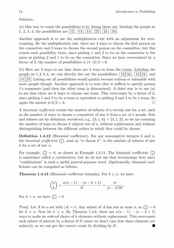
A binomial coe�cient counts the number of subsets of a certain size for a set, suchas the number of ways to choose a committee of size k from a set of n people. Setsand subsets are by definition unordered, e.g., {3, 1, 4} = {4, 1, 3}, so we are countingthe number of ways to choose k objects out of n, without replacement and withoutdistinguishing between the di↵erent orders in which they could be chosen.
Definition 1.4.12 (Binomial coe�cient). For any nonnegative integers k and n,the binomial coe�cient
�nk
�, read as “n choose k”, is the number of subsets of size
k for a set of size n.
For example,�4
2
�= 6, as shown in Example 1.4.11. The binomial coe�cient
�nk
�
is sometimes called a combination, but we do not use that terminology here since“combination” is such a useful general-purpose word. Algebraically, binomial coef-ficients can be computed as follows.
Theorem 1.4.13 (Binomial coe�cient formula). For k n, we have
✓n
k
◆=
n(n� 1) · · · (n� k + 1)
k!=
n!
(n� k)!k!.
For k > n, we have�nk
�= 0.
Proof. Let A be a set with |A| = n. Any subset of A has size at most n, so�nk
�= 0
for k > n. Now let k n. By Theorem 1.4.6, there are n(n � 1) · · · (n � k + 1)ways to make an ordered choice of k elements without replacement. This overcountseach subset of interest by a factor of k! (since we don’t care how these elements areordered), so we can get the correct count by dividing by k!. ⌅

Probability and counting 15
h 1.4.14. The binomial coe�cient�nk
�is often defined in terms of factorials, but
keep in mind that�nk
�is 0 if k > n, even though the factorial of a negative number
is undefined. Also, the middle expression in Theorem 1.4.13 is often better forcomputation than the expression with factorials, since factorials grow extremelyfast. For example, ✓
100
2
◆=
100 · 992
= 4950
can even be done by hand, whereas computing�100
2
�= 100!/(98!·2!) by first calculat-
ing 100! and 98! would be wasteful and possibly dangerous because of the extremelylarge numbers involved (100! ⇡ 9.33⇥ 10157).
Example 1.4.15 (Club o�cers). In a club with n people, there are n(n�1)(n�2)ways to choose a president, vice president, and treasurer, and there are
�n3
�=
n(n�1)(n�2)
3!
ways to choose 3 o�cers without predetermined titles. ⇤Example 1.4.16 (Permutations of a word). How many ways are there to permutethe letters in the word LALALAAA? To determine a permutation, we just need tochoose where the 5 A’s go (or, equivalently, just decide where the 3 L’s go). So thereare ✓
8
5
◆=
✓8
3
◆=
8 · 7 · 63!
= 56 permutations.
How many ways are there to permute the letters in the word STATISTICS? Hereare two approaches. We could choose where to put the S’s, then where to put theT’s (from the remaining positions), then where to put the I’s, then where to putthe A (and then the C is determined). Alternatively, we can start with 10! and thenadjust for overcounting, dividing by 3!3!2! to account for the fact that the S’s canbe permuted among themselves in any way, and likewise for the T’s and I’s. Thisgives ✓
10
3
◆✓7
3
◆✓4
2
◆✓2
1
◆=
10!
3!3!2!= 50400 possibilities.
⇤Example 1.4.17 (Binomial theorem). The binomial theorem states that
(x+ y)n =nX
k=0
✓n
k
◆xkyn�k.
To prove the binomial theorem, expand out the product
(x+ y)(x+ y) . . . (x+ y)| {z }n factors
.
Just as (a+ b)(c+ d) = ac+ ad+ bc+ bd is the sum of terms where we pick the a orthe b from the first factor (but not both) and the c or the d from the second factor(but not both), the terms of (x+ y)n are obtained by picking either the x or the y(but not both) from each factor. There are
�nk
�ways to choose exactly k of the x’s,
and each such choice yields the term xkyn�k. The binomial theorem follows. ⇤

16 Introduction to Probability
We can use binomial coe�cients to calculate probabilities in many problems forwhich the naive definition applies.
Example 1.4.18 (Full house in poker). A 5-card hand is dealt from a standard,well-shu✏ed 52-card deck. The hand is called a full house in poker if it consists ofthree cards of some rank and two cards of another rank, e.g., three 7’s and two 10’s(in any order). What is the probability of a full house?
Solution:
All of the�52
5
�possible hands are equally likely by symmetry, so the naive definition
is applicable. To find the number of full house hands, use the multiplication rule(and imagine the tree). There are 13 choices for what rank we have three of; forconcreteness, assume we have three 7’s and focus on that branch of the tree. Thereare
�4
3
�ways to choose which 7’s we have. Then there are 12 choices for what rank
we have two of, say 10’s for concreteness, and�4
2
�ways to choose two 10’s. Thus,
P (full house) =13�4
3
�12�4
2
��52
5
� =3744
2598960⇡ 0.00144.
The decimal approximation is more useful when playing poker, but the answer interms of binomial coe�cients is exact and self-annotating (seeing “
�52
5
�” is a much
bigger hint of its origin than seeing “2598960”). ⇤Example 1.4.19 (Newton-Pepys problem). Isaac Newton was consulted aboutthe following problem by Samuel Pepys, who wanted the information for gamblingpurposes. Which of the following events has the highest probability?
A: At least one 6 appears when 6 fair dice are rolled.
B: At least two 6’s appear when 12 fair dice are rolled.
C: At least three 6’s appear when 18 fair dice are rolled.
Solution:
The three experiments have 66, 612, and 618 possible outcomes, respectively, and bysymmetry the naive definition applies in all three experiments.
A: Instead of counting the number of ways to obtain at least one 6, it is easier tocount the number of ways to get no 6’s. Getting no 6’s is equivalent to sampling thenumbers 1 through 5 with replacement 6 times, so 56 outcomes are favorable to Ac
(and 66 � 56 are favorable to A). Thus
P (A) = 1� 56
66⇡ 0.67.
B: Again we count the outcomes in Bc first. There are 512 ways to get no 6’s in12 die rolls. There are
�12
1
�511 ways to get exactly one 6: we first choose which die

Probability and counting 17
lands 6, then sample the numbers 1 through 5 with replacement for the other 11dice. Adding these, we get the number of ways to fail to obtain at least two 6’s.Then
P (B) = 1�512 +
�12
1
�511
612⇡ 0.62.
C: We count the outcomes in Cc, i.e., the number of ways to get zero, one, or two6’s in 18 die rolls. There are 518 ways to get no 6’s,
�18
1
�517 ways to get exactly one
6, and�18
2
�516 ways to get exactly two 6’s (choose which two dice will land 6, then
decide how the other 16 dice will land).
P (C) = 1�518 +
�18
1
�517 +
�18
2
�516
618⇡ 0.60.
Therefore A has the highest probability.
Newton arrived at the correct answer using similar calculations. Newton also pro-vided Pepys with an intuitive argument for why A was the most likely of the three;however, his intuition was invalid. As explained in Stigler [27], using loaded dicecould result in a di↵erent ordering of A,B,C, but Newton’s intuitive argument didnot depend on the dice being fair. ⇤In this book, we care about counting not for its own sake, but because it sometimeshelps us to find probabilities. Here is an example of a neat but treacherous countingproblem; the solution is elegant, but it is rare that the result can be used with thenaive definition of probability.
Example 1.4.20 (Bose-Einstein). How many ways are there to choose k times froma set of n objects with replacement, if order doesn’t matter (we only care abouthow many times each object was chosen, not the order in which they were chosen)?
Solution:
When order does matter, the answer is nk by the multiplication rule, but thisproblem is much harder. We will solve it by solving an isomorphic problem (thesame problem in a di↵erent guise).
Let us find the number of ways to put k indistinguishable particles into n distin-guishable boxes. That is, swapping the particles in any way is not considered aseparate possibility: all that matters are the counts for how many particles are ineach box. Any configuration can be encoded as a sequence of |’s and l’s in a naturalway, as illustrated in Figure 1.5.
To be valid, a sequence must start and end with a |, with exactly n�1 |’s and k l’sin between; conversely, any such sequence is a valid encoding for some configurationof particles in boxes. Thus there are n + k � 1 slots between the two outer walls,and we need only choose where to put the k l’s, so the number of possibilities is�n+k�1
k
�. This is known as the Bose-Einstein value, since the physicists Satyenda
Nath Bose and Albert Einstein studied related problems about indistinguishable

18 Introduction to Probability
FIGURE 1.5
Bose-Einstein encoding: putting k = 7 indistinguishable particles into n = 4 distin-guishable boxes can be expressed as a sequence of |’s and l’s, where | denotes awall and l denotes a particle.
particles in the 1920s, using their ideas to successfully predict the existence of astrange state of matter known as a Bose-Einstein condensate.
To relate this back to the original question, we can let each box correspond to oneof the n objects and use the particles as “check marks” to tally how many timeseach object is selected. For example, if a certain box contains exactly 3 particles,that means the object corresponding to that box was chosen exactly 3 times. Theparticles being indistinguishable corresponds to the fact that we don’t care aboutthe order in which the objects are chosen. Thus, the answer to the original questionis also
�n+k�1
k
�.
Another isomorphic problem is to count the number of solutions (x1
, . . . , xn) to theequation x
1
+ x2
+ · · · + xn = k, where the xi are nonnegative integers. This isequivalent since we can think of xi as the number of particles in the ith box.
h 1.4.21. The Bose-Einstein result should not be used in the naive definition ofprobability except in very special circumstances. For example, consider a surveywhere a sample of size k is collected by choosing people from a population of size none at a time, with replacement and with equal probabilities. Then the nk orderedsamples are equally likely, making the naive definition applicable, but the
�n+k�1
k
�
unordered samples (where all that matters is how many times each person wassampled) are not equally likely.
As another example, with n = 365 days in a year and k people, how many possibleunordered birthday lists are there? For example, for k = 3, we want to count listslike (May 1, March 31, April 11), where all permutations are considered equivalent.We can’t do a simple adjustment for overcounting such as nk/3! since, e.g., there are6 permutations of (May 1, March 31, April 11) but only 3 permutations of (March31, March 31, April 11). By Bose-Einstein, the number of lists is
�n+k�1
k
�. But the
ordered birthday lists are equally likely, not the unordered lists, so the Bose-Einsteinvalue should not be used in calculating birthday probabilities.
⇤

Probability and counting 19
1.5 Story proofs
A story proof is a proof by interpretation. For counting problems, this often meanscounting the same thing in two di↵erent ways, rather than doing tedious algebra. Astory proof often avoids messy calculations and goes further than an algebraic prooftoward explaining why the result is true. The word “story” has several meanings,some more mathematical than others, but a story proof (in the sense in which we’reusing the term) is a fully valid mathematical proof. Here are some examples of storyproofs, which also serve as further examples of counting.
Example 1.5.1 (Choosing the complement). For any nonnegative integers n andk with k n, we have ✓
n
k
◆=
✓n
n� k
◆.
This is easy to check algebraically (by writing the binomial coe�cients in terms offactorials), but a story proof makes the result easier to understand intuitively.
Story proof : Consider choosing a committee of size k in a group of n people. Weknow that there are
�nk
�possibilities. But another way to choose the committee is
to specify which n � k people are not on the committee; specifying who is on thecommittee determines who is not on the committee, and vice versa. So the two sidesare equal, as they are two ways of counting the same thing. ⇤Example 1.5.2 (The team captain). For any positive integers n and k with k n,
n
✓n� 1
k � 1
◆= k
✓n
k
◆.
This is again easy to check algebraically (using the fact that m! = m(m � 1)! forany positive integer m), but a story proof is more insightful.
Story proof : Consider a group of n people, from which a team of k will be chosen,one of whom will be the team captain. To specify a possibility, we could first choosethe team captain and then choose the remaining k � 1 team members; this givesthe left-hand side. Equivalently, we could first choose the k team members and thenchoose one of them to be captain; this gives the right-hand side. ⇤Example 1.5.3 (Vandermonde’s identity). A famous relationship between binomialcoe�cients, called Vandermonde’s identity, says that
✓m+ n
k
◆=
kX
j=0
✓m
j
◆✓n
k � j
◆.
This identity will come up several times in this book. Trying to prove it with abrute force expansion of all the binomial coe�cients would be a nightmare. But astory proves the result elegantly and makes it clear why the identity holds.

20 Introduction to Probability
Story proof : Consider a group of m men and n women, from which a committeeof size k will be chosen. There are
�m+nk
�possibilities. If there are j men in the
committee, then there must be k� j women in the committee. The right-hand sideof Vandermonde’s identity sums up the cases for j. ⇤
Example 1.5.4 (Partnerships). Let’s use a story proof to show that
(2n)!
2n · n! = (2n� 1)(2n� 3) · · · 3 · 1.
Story proof : We will show that both sides count the number of ways to break 2npeople into n partnerships. Take 2n people, and give them ID numbers from 1 to2n. We can form partnerships by lining up the people in some order and then sayingthe first two are a pair, the next two are a pair, etc. This overcounts by a factorof n! · 2n since the order of pairs doesn’t matter, nor does the order within eachpair. Alternatively, count the number of possibilities by noting that there are 2n�1choices for the partner of person 1, then 2n� 3 choices for person 2 (or person 3, ifperson 2 was already paired to person 1), and so on. ⇤
1.6 Non-naive definition of probability
We have now seen several methods for counting outcomes in a sample space, allowingus to calculate probabilities if the naive definition applies. But the naive definitioncan only take us so far, since it requires equally likely outcomes and can’t handlean infinite sample space. To generalize the notion of probability, we’ll use the bestpart about math, which is that you get to make up your own definitions. Whatthis means is that we write down a short wish list of how we want probability tobehave (in math, the items on the wish list are called axioms), and then we definea probability function to be something that satisfies the properties we want!
Here is the general definition of probability that we’ll use for the rest of this book.It requires just two axioms, but from these axioms it is possible to prove a vastarray of results about probability.
Definition 1.6.1 (General definition of probability). A probability space consistsof a sample space S and a probability function P which takes an event A ✓ S asinput and returns P (A), a real number between 0 and 1, as output. The functionP must satisfy the following axioms:
1. P (;) = 0, P (S) = 1.

Probability and counting 21
2. If A1
, A2
, . . . are disjoint events, then
P
0
@1[
j=1
Aj
1
A =1X
j=1
P (Aj).
(Saying that these events are disjoint means that they are mutually exclu-sive: Ai \Aj = ; for i 6= j.)
In Pebble World, the definition says that probability behaves like mass: the massof an empty pile of pebbles is 0, the total mass of all the pebbles is 1, and if wehave non-overlapping piles of pebbles, we can get their combined mass by addingthe masses of the individual piles. Unlike in the naive case, we can now have pebblesof di↵ering masses, and we can also have a countably infinite number of pebbles aslong as their total mass is 1.
We can even have uncountable sample spaces, such as having S be an area in theplane. In this case, instead of pebbles, we can visualize mud spread out over a region,where the total mass of the mud is 1.
Any function P (mapping events to numbers in the interval [0, 1]) that satisfies thetwo axioms is considered a valid probability function. However, the axioms don’t tellus how probability should be interpreted ; di↵erent schools of thought exist.
The frequentist view of probability is that it represents a long-run frequency over alarge number of repetitions of an experiment: if we say a coin has probability 1/2 ofHeads, that means the coin would land Heads 50% of the time if we tossed it overand over and over.
The Bayesian view of probability is that it represents a degree of belief about theevent in question, so we can assign probabilities to hypotheses like “candidate Awill win the election” or “the defendant is guilty” even if it isn’t possible to repeatthe same election or the same crime over and over again.
The Bayesian and frequentist perspectives are complementary, and both will behelpful for developing intuition in later chapters. Regardless of how we choose tointerpret probability, we can use the two axioms to derive other properties of prob-ability, and these results will hold for any valid probability function.
Theorem 1.6.2 (Properties of probability). Probability has the following proper-ties, for any events A and B.
1. P (Ac) = 1� P (A).
2. If A ✓ B, then P (A) P (B).
3. P (A [B) = P (A) + P (B)� P (A \B).

22 Introduction to Probability
Proof.
1. Since A and Ac are disjoint and their union is S, the second axiom gives
P (S) = P (A [Ac) = P (A) + P (Ac),
But P (S) = 1 by the first axiom. So P (A) + P (Ac) = 1.
2. If A ✓ B, then we can write B as the union of A and B \ Ac, where B \ Ac isthe part of B not also in A. This is illustrated in the figure below.
S
AB
B ∩ Ac
Since A and B \Ac are disjoint, we can apply the second axiom:
P (B) = P (A [ (B \Ac)) = P (A) + P (B \Ac).
Probability is nonnegative, so P (B \Ac) � 0, proving that P (B) � P (A).
3. The intuition for this result can be seen using a Venn diagram like the one below.
S
A B
A ∩ B
The shaded region represents A[B, but the probability of this region is not P (A)+P (B), because that would count the football-shaped region A\B twice. To correctfor this, we subtract P (A \B). This is a useful intuition, but not a proof.
For a proof using the axioms of probability, we can write A[B as the union of thedisjoint events A and B \Ac. Then by the second axiom,
P (A [B) = P (A [ (B \Ac)) = P (A) + P (B \Ac).
So it su�ces to show that P (B \Ac) = P (B)�P (A\B). Since A\B and B \Ac
are disjoint and their union is B, another application of the second axiom gives us
P (A \B) + P (B \Ac) = P (B).
So P (B \Ac) = P (B)� P (A \B), as desired. ⌅

Probability and counting 23
The third property is a special case of inclusion-exclusion, a formula for finding theprobability of a union of events when the events are not necessarily disjoint. Weshowed above that for two events A and B,
P (A [B) = P (A) + P (B)� P (A \B).
For three events, inclusion-exclusion says
P (A [B [ C) = P (A) + P (B) + P (C)
� P (A \B)� P (A \ C)� P (B \ C)
+ P (A \B \ C).
For intuition, consider a triple Venn diagram like the one below.
A B
C
To get the total area of the shaded region A [B [C, we start by adding the areasof the three circles, P (A) + P (B) + P (C). The three football-shaped regions haveeach been counted twice, so we then subtract P (A \ B) + P (A \ C) + P (B \ C).Finally, the region in the center has been added three times and subtracted threetimes, so in order to count it exactly once, we must add it back again. This ensuresthat each region of the diagram has been counted once and exactly once.
Now we can write inclusion-exclusion for n events.
Theorem 1.6.3 (Inclusion-exclusion). For any events A1
, . . . , An,
P
n[
i=1
Ai
!=X
i
P (Ai)�X
i<j
P (Ai \Aj) +X
i<j<k
P (Ai \Aj \Ak)� . . .
+ (�1)n+1P (A1
\ · · · \An).
This formula can be proven by induction using just the axioms, but instead we’llpresent a shorter proof in Chapter 4 after introducing some additional tools. Therationale behind the alternating addition and subtraction in the general formula isanalogous to the special cases we’ve already considered.
The next example, de Montmort’s matching problem, is a famous application ofinclusion-exclusion. Pierre Remond de Montmort was a French mathematician whostudied probability in the context of gambling and wrote a treatise [21] devoted tothe analysis of various card games. He posed the following problem in 1708, basedon a card game called Treize.

24 Introduction to Probability
Example 1.6.4 (de Montmort’s matching problem). Consider a well-shu✏ed deckof n cards, labeled 1 through n. You flip over the cards one by one, saying thenumbers 1 through n as you do so. You win the game if, at some point, the numberyou say aloud is the same as the number on the card being flipped over (for example,if the 7th card in the deck has the label 7). What is the probability of winning?
Solution:
Let Ai be the event that the ith card in the deck has the number i written on it.We are interested in the probability of the union A
1
[ · · · [ An: as long as at leastone of the cards has a number matching its position in the deck, you will win thegame. (An ordering for which you lose is called a derangement, though hopefully noone has ever become deranged due to losing at this game.)
To find the probability of the union, we’ll use inclusion-exclusion. First,
P (Ai) =1
n
for all i. One way to see this is with the naive definition of probability, using thefull sample space: there are n! possible orderings of the deck, all equally likely, and(n�1)! of these are favorable to Ai (fix the card numbered i to be in the ith positionin the deck, and then the remaining n� 1 cards can be in any order). Another wayto see this is by symmetry: the card numbered i is equally likely to be in any of then positions in the deck, so it has probability 1/n of being in the ith spot. Second,
P (Ai \Aj) =(n� 2)!
n!=
1
n(n� 1),
since we require the cards numbered i and j to be in the ith and jth spots in thedeck and allow the remaining n � 2 cards to be in any order, so (n � 2)! out of n!possibilities are favorable to Ai \Aj . Similarly,
P (Ai \Aj \Ak) =1
n(n� 1)(n� 2),
and the pattern continues for intersections of 4 events, etc.
In the inclusion-exclusion formula, there are n terms involving one event,�n2
�terms
involving two events,�n3
�terms involving three events, and so forth. By the sym-
metry of the problem, all n terms of the form P (Ai) are equal, all�n2
�terms of the
form P (Ai \Aj) are equal, and the whole expression simplifies considerably:
P
n[
i=1
Ai
!=
n
n�
�n2
�
n(n� 1)+
�n3
�
n(n� 1)(n� 2)� · · ·+ (�1)n+1 · 1
n!
= 1� 1
2!+
1
3!� · · ·+ (�1)n+1 · 1
n!.
Comparing this to the Taylor series for 1/e (see Section A.8 of the math appendix),
e�1 = 1� 1
1!+
1
2!� 1
3!+ . . . ,

Probability and counting 25
we see that for large n, the probability of winning the game is extremely closeto 1 � 1/e, or about 0.63. Interestingly, as n grows, the probability of winningapproaches 1 � 1/e instead of going to 0 or 1. With a lot of cards in the deck, thenumber of possible locations for matching cards increases while the probability ofany particular match decreases, and these two forces o↵set each other and balanceto give a probability of about 1� 1/e. ⇤
Inclusion-exclusion is a very general formula for the probability of a union of events,but it helps us the most when there is symmetry among the events Aj ; otherwisethe sum can be extremely tedious. In general, when symmetry is lacking, we shouldtry to use other tools before turning to inclusion-exclusion as a last resort.
1.7 Recap
Probability allows us to quantify uncertainty and randomness in a principled way.Probabilities arise when we perform an experiment: the set of all possible outcomesof the experiment is called the sample space, and a subset of the sample spaceis called an event. It is useful to be able to go back and forth between describingevents in English and writing them down mathematically as sets (often using unions,intersections, and complements).
Pebble World can help us visualize sample spaces and events when the sample spaceis finite. In Pebble World, each outcome is a pebble, and an event is a set of pebbles.If all the pebbles have the same mass (i.e., are equally likely), we can apply the naivedefinition of probability, which lets us calculate probabilities by counting.
To this end, we discussed several tools for counting. When counting the numberof possibilities, we often use the multiplication rule. If we can’t directly use themultiplication rule, we can sometimes count each possibility exactly c times forsome c, and then divide by c to get the actual number of possibilities.
An important pitfall to avoid is misapplying the naive definition of probability,implicitly or explicitly assuming equally likely outcomes without justification. Onetechnique to help avoid this is to give objects labels, for precision and so that we arenot tempted to treat them as indistinguishable.
Moving beyond the naive definition, we define probability to be a function thattakes an event and assigns to it a real number between 0 and 1. We require a validprobability function to satisfy two axioms:
1. P (;) = 0, P (S) = 1.
2. If A1
, A2
, . . . are disjoint events, then P
0
@1[
j=1
Aj
1
A =1X
j=1
P (Aj).

26 Introduction to Probability
Many useful properties can be derived just from these axioms. For example,
P (Ac) = 1� P (A)
for any event A, and we have the inclusion-exclusion formula
P
n[
i=1
Ai
!=X
i
P (Ai)�X
i<j
P (Ai \Aj) +X
i<j<k
P (Ai \Aj \Ak)� . . .
+ (�1)n+1P (A1
\ · · · \An)
for any events A1
, . . . , An. For n = 2, this is the much nicer-looking result
P (A1
[A2
) = P (A1
) + P (A2
)� P (A1
\A2
).
Figure 1.6 illustrates how a probability function maps events to numbers between0 and 1. We’ll add many new concepts to this diagram as we continue our journeythrough the field of probability.
events numbersP(A)
P(Ac) = 1 – P(A) P(A⋂B)
P(A⋃B) = P(A) + P(B) – P(A⋂B)P(S) = 1
Anot A
A and BA or B
something happened
What can happen?
P
FIGURE 1.6
It is important to distinguish between events and probabilities. The former are sets,while the latter are numbers. Before the experiment is done, we generally don’t knowwhether or not a particular event will occur (happen). So we assign it a probabilityof happening, using a probability function P . We can use set operations to definenew events in terms of old events, and the properties of probabilities to relate theprobabilities of the new events to those of the old events.

Probability and counting 27
1.8 R
R is a very powerful, popular environment for statistical computing and graphics,freely available for Mac OS X, Windows, and UNIX systems. Knowing how to use Ris an extremely useful skill. R and various supporting information can be obtainedat http://www.r-project.org. RStudio is an alternative interface for R, freelyavailable at http://www.rstudio.com.
In the R section at the end of each chapter, we provide R code to let you try outsome of the examples from the chapter, especially via simulation. These sectionsare not intended to be a full introduction to R; many R tutorials are availablefor free online, and many books on R are available. But the R sections show howto implement various simulations, computations, and visualizations that naturallyaccompany the material from each chapter.
Vectors
R is built around vectors, and getting familiar with “vectorized thinking” is veryimportant for using R e↵ectively. To create a vector, we can use the c command(which stands for combine or concatenate). For example,
v <- c(3,1,4,1,5,9)
defines v to be the vector (3, 1, 4, 1, 5, 9). (The left arrow <- is typed as < followedby -. The symbol = can be used instead, but the arrow is more suggestive of the factthat the variable on the left is being set equal to the value on the right.) Similarly,n <- 110 sets n equal to 110; R views n as a vector of length 1.
sum(v)
adds up the entries of v, max(v) gives the largest value, min(v) gives the smallestvalue, and length(v) gives the length.
A shortcut for getting the vector (1, 2, . . . , n) is to type 1:n; more generally, if mand n are integers then m:n gives the sequence of integers from m to n (in increasingorder if m n and in decreasing order otherwise).
To access the ith entry of a vector v, use v[i]. We can also get subvectors eas-ily:
v[c(1,3,5)]
gives the vector consisting of the 1st, 3rd, and 5th entries of v. It’s also possible toget a subvector by specifying what to exclude, using a minus sign:
v[-(2:4)]

28 Introduction to Probability
gives the vector obtained by removing the 2nd through 4th entries of v (the paren-theses are needed since -2:4 would be (�2,�1, . . . , 4)).
Many operations in R are interpreted componentwise. For example, in math thecube of a vector doesn’t have a standard definition, but in R typing v^3 simplycubes each entry individually. Similarly,
1/(1:100)^2
is a very compact way to get the vector (1, 1
2
2
, 1
3
2
, . . . , 1
100
2
).
In math, v+w is undefined if v and w are vectors of di↵erent lengths, but in R theshorter vector gets “recycled”! For example, v+3 adds 3 to each entry of v.
Factorials and binomial coe�cients
We can compute n! using factorial(n) and�nk
�using choose(n,k). As we have
seen, factorials grow extremely quickly. What is the largest n for which R returns anumber for factorial(n)? Beyond that point, R will return Inf (infinity), with awarning message. But it may still be possible to use lfactorial(n) for larger valuesof n, which computes log(n!). Similarly, lchoose(n,k) computes log
�nk
�.
Sampling and simulation
The sample command is a useful way of drawing random samples in R. (Techni-cally, they are pseudo-random since there is an underlying deterministic algorithm,but they “look like” random samples for almost all practical purposes.) For exam-ple,
n <- 10; k <- 5
sample(n,k)
generates an ordered random sample of 5 of the numbers from 1 to 10, withoutreplacement, and with equal probabilities given to each number. To sample withreplacement instead, just add in replace = TRUE:
n <- 10; k <- 5
sample(n,k,replace=TRUE)
To generate a random permutation of 1, 2, . . . , n we can use sample(n,n), whichbecause of R’s default settings can be abbreviated to sample(n).
We can also use sample to draw from a non-numeric vector. For example, letters isbuilt into R as the vector consisting of the 26 lowercase letters of the English alpha-bet, and sample(letters,7) will generate a random 7-letter “word” by samplingfrom the alphabet, without replacement.

Probability and counting 29
The sample command also allows us to specify general probabilities for samplingeach number. For example,
sample(4, 3, replace=TRUE, prob=c(0.1,0.2,0.3,0.4))
samples 3 numbers between 1 and 4, with replacement, and with probabilities givenby (0.1, 0.2, 0.3, 0.4). If the sampling is without replacement, then at each stage theprobability of any not-yet-chosen number is proportional to its original probabil-ity.
Generating many random samples allows us to perform a simulation for a proba-bility problem. The replicate command, which is explained below, is a convenientway to do this.
Matching problem simulation
Let’s show by simulation that the probability of a matching card in Example 1.6.4 isapproximately 1� 1/e when the deck is su�ciently large. Using R, we can performthe experiment a bunch of times and see how many times we encounter at least onematching card:
n <- 100
r <- replicate(10^4,sum(sample(n)==(1:n)))
sum(r>=1)/10^4
In the first line, we choose how many cards are in the deck (here, 100 cards). In thesecond line, let’s work from the inside out:
• sample(n)==(1:n) is a vector of length n, the ith element of which equals 1 if theith card matches its position in the deck and 0 otherwise. That’s because for twonumbers a and b, the expression a==b is TRUE if a = b and FALSE otherwise,and TRUE is encoded as 1 and FALSE is encoded as 0.
• sum adds up the elements of the vector, giving us the number of matching cardsin this run of the experiment.
• replicate does this 104 times. We store the results in r, a vector of length 104
containing the numbers of matched cards from each run of the experiment.
In the last line, we add up the number of times where there was at least one matchingcard, and we divide by the number of simulations.
To explain what the code is doing within the code rather than in separate documen-tation, we can add comments using the # symbol to mark the start of a comment.Comments are ignored by R but can make the code much easier to understand forthe reader (who could be you—even if you will be the only one using your code, itis often hard to remember what everything means and how the code is supposed towork when looking at it a month after writing it). Short comments can be on the

30 Introduction to Probability
same line as the corresponding code; longer comments should be on separate lines.For example, a commented version of the above simulation is:
n <- 100 # number of cards
r <- replicate(10^4,sum(sample(n)==(1:n))) # shuffle; count matches
sum(r>=1)/10^4 # proportion with a match
What did you get when you ran the code? We got 0.63, which is quite close to1� 1/e.
Birthday problem calculation and simulation
The following code uses prod (which gives the product of a vector) to calculate theprobability of at least one birthday match in a group of 23 people:
k <- 23
1-prod((365-k+1):365)/365^k
Better yet, R has built-in functions, pbirthday and qbirthday, for the birthdayproblem! pbirthday(k) returns the probability of at least one match if the roomhas k people. qbirthday(p) returns the number of people needed in order to haveprobability p of at least one match. For example, pbirthday(23) is 0.507 andqbirthday(0.5) is 23.
We can also find the probability of having at least one triple birthday match, i.e.,three people with the same birthday; all we have to do is add coincident=3 tosay we’re looking for triple matches. For example, pbirthday(23,coincident=3)returns 0.014, so 23 people give us only a 1.4% chance of a triple birthday match.qbirthday(0.5,coincident=3) returns 88, so we’d need 88 people to have at leasta 50% chance of at least one triple birthday match.
To simulate the birthday problem, we can use
b <- sample(1:365,23,replace=TRUE)
tabulate(b)
to generate random birthdays for 23 people and then tabulate the counts of howmany people were born on each day (the command table(b) creates a prettiertable, but is slower). We can run 104 repetitions as follows:
r <- replicate(10^4, max(tabulate(sample(1:365,23,replace=TRUE))))
sum(r>=2)/10^4
If the probabilities of various days are not all equal, the calculation becomes muchmore di�cult, but the simulation can easily be extended since sample allows us tospecify the probability of each day (by default sample assigns equal probabilities,so in the above the probability is 1/365 for each day).

Probability and counting 31
1.9 Exercises
Exercises marked with s� throughout this book have detailed solutions online atstat110.net. We highly recommend working on the exercises yourself before study-ing the online solutions.
Counting
1. How many ways are there to permute the letters in the word MISSISSIPPI?
2. (a) How many 7-digit phone numbers are possible, assuming that the first digit can’tbe a 0 or a 1?
(b) Re-solve (a), except now assume also that the phone number is not allowed to startwith 911 (since this is reserved for emergency use, and it would not be desirable for thesystem to wait to see whether more digits were going to be dialed after someone hasdialed 911).
3. Fred is planning to go out to dinner each night of a certain week, Monday throughFriday, with each dinner being at one of his ten favorite restaurants.
(a) How many possibilities are there for Fred’s schedule of dinners for that Mondaythrough Friday, if Fred is not willing to eat at the same restaurant more than once?
(b) How many possibilities are there for Fred’s schedule of dinners for that Mondaythrough Friday, if Fred is willing to eat at the same restaurant more than once, but isnot willing to eat at the same place twice in a row (or more)?
4. A round-robin tournament is being held with n tennis players; this means that everyplayer will play against every other player exactly once.
(a) How many possible outcomes are there for the tournament (the outcome lists outwho won and who lost for each game)?
(b) How many games are played in total?
5. A knock-out tournament is being held with 2n tennis players. This means that for eachround, the winners move on to the next round and the losers are eliminated, until onlyone person remains. For example, if initially there are 24 = 16 players, then there are8 games in the first round, then the 8 winners move on to round 2, then the 4 winnersmove on to round 3, then the 2 winners move on to round 4, the winner of which isdeclared the winner of the tournament. (There are various systems for determining whoplays whom within a round, but these do not matter for this problem.)
(a) How many rounds are there?
(b) Count how many games in total are played, by adding up the numbers of gamesplayed in each round.
(c) Count how many games in total are played, this time by directly thinking about itwithout doing almost any calculation.
Hint: How many players need to be eliminated?
6. There are 20 people at a chess club on a certain day. They each find opponents andstart playing. How many possibilities are there for how they are matched up, assumingthat in each game it does matter who has the white pieces (in a chess game, one playerhas the white pieces and the other player has the black pieces)?

32 Introduction to Probability
7. Two chess players, A and B, are going to play 7 games. Each game has three possibleoutcomes: a win for A (which is a loss for B), a draw (tie), and a loss for A (which isa win for B). A win is worth 1 point, a draw is worth 0.5 points, and a loss is worth 0points.
(a) How many possible outcomes for the individual games are there, such that overallplayer A ends up with 3 wins, 2 draws, and 2 losses?
(b) How many possible outcomes for the individual games are there, such that A endsup with 4 points and B ends up with 3 points?
(c) Now assume that they are playing a best-of-7 match, where the match will end assoon as either player has 4 points. For example, if after 6 games the score is 4 to 2 infavor of A, then A wins the match and they don’t play a 7th game. How many possibleoutcomes for the individual games are there, such that the match lasts for 7 games andA wins by a score of 4 to 3?
8. s� (a) How many ways are there to split a dozen people into 3 teams, where one teamhas 2 people, and the other two teams have 5 people each?
(b) How many ways are there to split a dozen people into 3 teams, where each team has4 people?
9. s� (a) How many paths are there from the point (0, 0) to the point (110, 111) in theplane such that each step either consists of going one unit up or one unit to the right?
(b) How many paths are there from (0, 0) to (210, 211), where each step consists of goingone unit up or one unit to the right, and the path has to go through (110, 111)?
10. To fulfill the requirements for a certain degree, a student can choose to take any 7 outof a list of 20 courses, with the constraint that at least 1 of the 7 courses must be astatistics course. Suppose that 5 of the 20 courses are statistics courses.
(a) How many choices are there for which 7 courses to take?
(b) Explain intuitively why the answer to (a) is not�5
1
�·�19
6
�.
11. Let A and B be sets with |A| = n, |B| = m.
(a) How many functions are there from A to B (i.e., functions with domain A, assigningan element of B to each element of A)?
(b) How many one-to-one functions are there from A to B (see Section A.2.1 of themath appendix for information about one-to-one functions)?
12. Four players, named A, B, C, and D, are playing a card game. A standard, well-shu✏eddeck of cards is dealt to the players (so each player receives a 13-card hand).
(a) How many possibilities are there for the hand that player A will get? (Within ahand, the order in which cards were received doesn’t matter.)
(b) How many possibilities are there overall for what hands everyone will get, assumingthat it matters which player gets which hand, but not the order of cards within a hand?
(c) Explain intuitively why the answer to Part (b) is not the fourth power of the answerto Part (a).
13. A certain casino uses 10 standard decks of cards mixed together into one big deck, whichwe will call a superdeck. Thus, the superdeck has 52 · 10 = 520 cards, with 10 copiesof each card. How many di↵erent 10-card hands can be dealt from the superdeck? Theorder of the cards does not matter, nor does it matter which of the original 10 decksthe cards came from. Express your answer as a binomial coe�cient.
Hint: Bose-Einstein.
14. You are ordering two pizzas. A pizza can be small, medium, large, or extra large, withany combination of 8 possible toppings (getting no toppings is allowed, as is getting all8). How many possibilities are there for your two pizzas?

Probability and counting 33
Story proofs
15. s� Give a story proof thatPn
k=0
�nk
�= 2n.
16. s� Show that for all positive integers n and k with n � k, n
k
!+
n
k � 1
!=
n+ 1k
!,
doing this in two ways: (a) algebraically and (b) with a story, giving an interpretationfor why both sides count the same thing.
Hint for the story proof: Imagine n + 1 people, with one of them pre-designated as“president”.
17. Give a story proof thatnX
k=1
k
n
k
!2
= n
2n� 1n� 1
!,
for all positive integers n.
Hint: Consider choosing a committee of size n from two groups of size n each, whereonly one of the two groups has people eligible to become president.
18. s� (a) Show using a story proof that k
k
!+
k + 1k
!+
k + 2k
!+ · · ·+
n
k
!=
n+ 1k + 1
!,
where n and k are positive integers with n � k. This is called the hockey stick identity.
Hint: Imagine arranging a group of people by age, and then think about the oldestperson in a chosen subgroup.
(b) Suppose that a large pack of Haribo gummi bears can have anywhere between 30and 50 gummi bears. There are 5 delicious flavors: pineapple (clear), raspberry (red),orange (orange), strawberry (green, mysteriously), and lemon (yellow). There are 0 non-delicious flavors. How many possibilities are there for the composition of such a pack ofgummi bears? You can leave your answer in terms of a couple binomial coe�cients, butnot a sum of lots of binomial coe�cients.
19. Define�nk
as the number of ways to partition {1, 2, . . . , n} into k non-empty subsets, or
the number of ways to have n students split up into k groups such that each group hasat least one student. For example,
�4
2
= 7 because we have the following possibilities:
• {1}, {2, 3, 4}• {2}, {1, 3, 4}• {3}, {1, 2, 4}• {4}, {1, 2, 3}
• {1, 2}, {3, 4}
• {1, 3}, {2, 4}
• {1, 4}, {2, 3}
Prove the following identities:
(a) (n+ 1k
)=
(n
k � 1
)+ k
(n
k
).
Hint: I’m either in a group by myself or I’m not.
(b)nX
j=k
n
j
!(j
k
)=
(n+ 1k + 1
).
Hint: First decide how many people are not going to be in my group.
34 Introduction to Probability
20. The Dutch mathematician R.J. Stroeker remarked:
Every beginning student of number theory surely must have marveled at the miraculousfact that for each natural number n the sum of the first n positive consecutive cubes isa perfect square. [29]
Furthermore, it is the square of the sum of the first n positive integers! That is,
13 + 23 + · · ·+ n3 = (1 + 2 + · · ·+ n)2.
Usually this identity is proven by induction, but that does not give much insight intowhy the result is true, nor does it help much if we wanted to compute the left-hand sidebut didn’t already know this result. In this problem, you will give a story proof of theidentity.
(a) Give a story proof of the identity
1 + 2 + · · ·+ n =
n+ 12
!.
Hint: Consider a round-robin tournament (see Exercise 4).
(b) Give a story proof of the identity
13 + 23 + · · ·+ n3 = 6
n+ 14
!+ 6
n+ 13
!+
n+ 12
!.
It is then just basic algebra (not required for this problem) to check that the square ofthe right-hand side in (a) is the right-hand side in (b).
Hint: Imagine choosing a number between 1 and n and then choosing 3 numbers between0 and n smaller than the original number, with replacement. Then consider cases basedon how many distinct numbers were chosen.
Naive definition of probability
21. Three people get into an empty elevator at the first floor of a building that has 10floors. Each presses the button for their desired floor (unless one of the others hasalready pressed that button). Assume that they are equally likely to want to go tofloors 2 through 10 (independently of each other). What is the probability that thebuttons for 3 consecutive floors are pressed?
22. s� A certain family has 6 children, consisting of 3 boys and 3 girls. Assuming that allbirth orders are equally likely, what is the probability that the 3 eldest children are the3 girls?
23. s� A city with 6 districts has 6 robberies in a particular week. Assume the robberies arelocated randomly, with all possibilities for which robbery occurred where equally likely.What is the probability that some district had more than 1 robbery?
24. A survey is being conducted in a city with 1 million residents. It would be far tooexpensive to survey all of the residents, so a random sample of size 1000 is chosen(in practice, there are many challenges with sampling, such as obtaining a completelist of everyone in the city, and dealing with people who refuse to participate). Thesurvey is conducted by choosing people one at a time, with replacement and with equalprobabilities.
(a) Explain how sampling with vs. without replacement here relates to the birthdayproblem.
(b) Find the probability that at least one person will get chosen more than once.
Probability and counting 35
25. A hash table is a commonly used data structure in computer science, allowing for fastinformation retrieval. For example, suppose we want to store some people’s phone num-bers. Assume that no two of the people have the same name. For each name x, a hashfunction h is used, letting h(x) be the location that will be used to store x’s phonenumber. After such a table has been computed, to look up x’s phone number one justrecomputes h(x) and then looks up what is stored in that location.
The hash function h is deterministic, since we don’t want to get di↵erent results everytime we compute h(x). But h is often chosen to be pseudorandom. For this problem,assume that true randomness is used. Let there be k people, with each person’s phonenumber stored in a random location (with equal probabilities for each location, inde-pendently of where the other people’s numbers are stored), represented by an integerbetween 1 and n. Find the probability that at least one location has more than onephone number stored there.
26. s� A college has 10 (non-overlapping) time slots for its courses, and blithely assignscourses to time slots randomly and independently. A student randomly chooses 3 of thecourses to enroll in. What is the probability that there is a conflict in the student’sschedule?
27. s� For each part, decide whether the blank should be filled in with =, <, or >, and givea clear explanation.
(a) (probability that the total after rolling 4 fair dice is 21) (probability that thetotal after rolling 4 fair dice is 22)
(b) (probability that a random 2-letter word is a palindrome2) (probability that arandom 3-letter word is a palindrome)
28. With definitions as in the previous problem, find the probability that a random n-letterword is a palindrome for n = 7 and for n = 8.
29. s� Elk dwell in a certain forest. There are N elk, of which a simple random sample ofsize n are captured and tagged (“simple random sample” means that all
�Nn
�sets of n
elk are equally likely). The captured elk are returned to the population, and then a newsample is drawn, this time with size m. This is an important method that is widely usedin ecology, known as capture-recapture. What is the probability that exactly k of the melk in the new sample were previously tagged? (Assume that an elk that was capturedbefore doesn’t become more or less likely to be captured again.)
30. Four cards are face down on a table. You are told that two are red and two are black, andyou need to guess which two are red and which two are black. You do this by pointingto the two cards you’re guessing are red (and then implicitly you’re guessing that theother two are black). Assume that all configurations are equally likely, and that you donot have psychic powers. Find the probability that exactly j of your guesses are correct,for j = 0, 1, 2, 3, 4.
31. s� A jar contains r red balls and g green balls, where r and g are fixed positive integers.A ball is drawn from the jar randomly (with all possibilities equally likely), and then asecond ball is drawn randomly.
(a) Explain intuitively why the probability of the second ball being green is the sameas the probability of the first ball being green.
(b) Define notation for the sample space of the problem, and use this to compute theprobabilities from (a) and show that they are the same.
2A palindrome is an expression such as “A man, a plan, a canal: Panama” that reads the samebackwards as forwards (ignoring spaces, capitalization, and punctuation). Assume for this problemthat all words of the specified length are equally likely, that there are no spaces or punctuation,and that the alphabet consists of the lowercase letters a,b,. . . ,z.
36 Introduction to Probability
(c) Suppose that there are 16 balls in total, and that the probability that the two ballsare the same color is the same as the probability that they are di↵erent colors. Whatare r and g (list all possibilities)?
32. s� A random 5-card poker hand is dealt from a standard deck of cards. Find the prob-ability of each of the following possibilities (in terms of binomial coe�cients).
(a) A flush (all 5 cards being of the same suit; do not count a royal flush, which is aflush with an ace, king, queen, jack, and 10).
(b) Two pair (e.g., two 3’s, two 7’s, and an ace).
33. A random 13-card hand is dealt from a standard deck of cards. What is the probabilitythat the hand contains at least 3 cards of every suit?
34. A group of 30 dice are thrown. What is the probability that 5 of each of the values1, 2, 3, 4, 5, 6 appear?
35. A deck of cards is shu✏ed well. The cards are dealt one by one, until the first time anAce appears.
(a) Find the probability that no kings, queens, or jacks appear before the first ace.
(b) Find the probability that exactly one king, exactly one queen, and exactly one kackappear (in any order) before the first ace.
36. Tyrion, Cersei, and ten other people are sitting at a round table, with their seatingarrangement having been randomly assigned. What is the probability that Tyrion andCersei are sitting next to each other? Find this in two ways:
(a) using a sample space of size 12!, where an outcome is fully detailed about the seating;
(b) using a much smaller sample space, which focuses on Tyrion and Cersei.
37. An organization with 2n people consists of n married couples. A committee of size k isselected, with all possibilities equally likely. Find the probability that there are exactlyj married couples within the committee.
38. There are n balls in a jar, labeled with the numbers 1, 2, . . . , n. A total of k balls aredrawn, one by one with replacement, to obtain a sequence of numbers.
(a) What is the probability that the sequence obtained is strictly increasing?
(b) What is the probability that the sequence obtained is increasing? (Note: In thisbook, “increasing” means “nondecreasing”.)
39. Each of n balls is independently placed into one of n boxes, with all boxes equally likely.What is the probability that exactly one box is empty?
40. s� A norepeatword is a sequence of at least one (and possibly all) of the usual 26 lettersa,b,c,. . . ,z, with repetitions not allowed. For example, “course” is a norepeatword, but“statistics” is not. Order matters, e.g., “course” is not the same as “source”.
A norepeatword is chosen randomly, with all norepeatwords equally likely. Show thatthe probability that it uses all 26 letters is very close to 1/e.
Axioms of probability
41. Show that for any events A and B,
P (A) + P (B)� 1 P (A \B) P (A [B) P (A) + P (B).
For each of these three inequalities, give a simple criterion for when the inequality isactually an equality (e.g., give a simple condition such that P (A \ B) = P (A [ B) ifand only if the condition holds).

Probability and counting 37
42. Let A and B be events. The di↵erence B �A is defined to be the set of all elements ofB that are not in A. Show that if A ✓ B, then
P (B �A) = P (B)� P (A),
directly using the axioms of probability.
43. Let A and B be events. The symmetric di↵erence A4B is defined to be the set of allelements that are in A or B but not both. In logic and engineering, this event is alsocalled the XOR (exclusive or) of A and B. Show that
P (A4B) = P (A) + P (B)� 2P (A \B),
directly using the axioms of probability.
44. Let A1
, A2
, . . . , An be events. Let Bk be the event that at least k of the Ai occur, andCk be the event that exactly k of the Ai occur, for 0 k n. Find a simple expressionfor P (Bk) in terms of P (Ck) and P (Ck+1
).
45. Events A and B are independent if P (A \ B) = P (A)P (B) (independence is exploredin detail in the next chapter).
(a) Give an example of independent events A and B in a finite sample space S (withneither equal to ; or S), and illustrate it with a Pebble World diagram.
(b) Consider the experiment of picking a random point in the rectangle
R = {(x, y) : 0 < x < 1, 0 < y < 1},
where the probability of the point being in any particular region contained within R isthe area of that region. Let A
1
and B1
be rectangles contained within R, with areas notequal to 0 or 1. Let A be the event that the random point is in A
1
, and B be the eventthat the random point is in B
1
. Give a geometric description of when it is true that Aand B are independent. Also, give an example where they are independent and anotherexample where they are not independent.
(c) Show that if A and B are independent, then
P (A [B) = P (A) + P (B)� P (A)P (B) = 1� P (Ac)P (Bc).
46. s� Arby has a belief system assigning a number PArby
(A) between 0 and 1 to every eventA (for some sample space). This represents Arby’s degree of belief about how likely Ais to occur. For any event A, Arby is willing to pay a price of 1000 · P
Arby
(A) dollars tobuy a certificate such as the one shown below:
Certificate
The owner of this certificate can redeem it for $1000 if A occurs. Novalue if A does not occur, except as required by federal, state, or locallaw. No expiration date.
Likewise, Arby is willing to sell such a certificate at the same price. Indeed, Arby iswilling to buy or sell any number of certificates at this price, as Arby considers it the“fair” price.
Arby stubbornly refuses to accept the axioms of probability. In particular, suppose thatthere are two disjoint events A and B with
PArby
(A [B) 6= PArby
(A) + PArby
(B).
Show how to make Arby go bankrupt, by giving a list of transactions Arby is willingto make that will guarantee that Arby will lose money (you can assume it will beknown whether A occurred and whether B occurred the day after any certificates arebought/sold).

38 Introduction to Probability
Inclusion-exclusion
47. A fair die is rolled n times. What is the probability that at least 1 of the 6 values neverappears?
48. s� A card player is dealt a 13-card hand from a well-shu✏ed, standard deck of cards.What is the probability that the hand is void in at least one suit (“void in a suit” meanshaving no cards of that suit)?
49. For a group of 7 people, find the probability that all 4 seasons (winter, spring, summer,fall) occur at least once each among their birthdays, assuming that all seasons are equallylikely.
50. A certain class has 20 students, and meets on Mondays and Wednesdays in a classroomwith exactly 20 seats. In a certain week, everyone in the class attends both days. Onboth days, the students choose their seats completely randomly (with one student perseat). Find the probability that no one sits in the same seat on both days of that week.
51. Fred needs to choose a password for a certain website. Assume that he will choose an8-character password, and that the legal characters are the lowercase letters a, b, c, . . . ,z, the uppercase letters A, B, C, . . . , Z, and the numbers 0, 1, . . . , 9.
(a) How many possibilities are there if he is required to have at least one lowercase letterin his password?
(b) How many possibilities are there if he is required to have at least one lowercaseletter and at least one uppercase letter in his password?
(c) How many possibilities are there if he is required to have at least one lowercaseletter, at least one uppercase letter, and at least one number in his password?
52. s� Alice attends a small college in which each class meets only once a week. She isdeciding between 30 non-overlapping classes. There are 6 classes to choose from for eachday of the week, Monday through Friday. Trusting in the benevolence of randomness,Alice decides to register for 7 randomly selected classes out of the 30, with all choicesequally likely. What is the probability that she will have classes every day, Mondaythrough Friday? (This problem can be done either directly using the naive definition ofprobability, or using inclusion-exclusion.)
53. A club consists of 10 seniors, 12 juniors, and 15 sophomores. An organizing committeeof size 5 is chosen randomly (with all subsets of size 5 equally likely).
(a) Find the probability that there are exactly 3 sophomores in the committee.
(b) Find the probability that the committee has at least one representative from eachof the senior, junior, and sophomore classes.
Mixed practice
54. For each part, decide whether the blank should be filled in with =, <, or >, and give aclear explanation. In (a) and (b), order doesn’t matter.
(a) (number of ways to choose 5 people out of 10) (number of ways to choose 6people out of 10)
(b) (number of ways to break 10 people into 2 teams of 5) (number of ways tobreak 10 people into a team of 6 and a team of 4)
(c) (probability that all 3 people in a group of 3 were born on January 1) (proba-bility that in a group of 3 people, 1 was born on each of January 1, 2, and 3)
Martin and Gale play an exciting game of “toss the coin,” where they toss a fair coinuntil the pattern HH occurs (two consecutive Heads) or the pattern TH occurs (Tails

Probability and counting 39
followed immediately by Heads). Martin wins the game if and only if HH occurs beforeTH occurs.
(d) (probability that Martin wins) 1/2
55. Take a deep breath before attempting this problem. In the book Innumeracy [22], JohnAllen Paulos writes:
Now for better news of a kind of immortal persistence. First, take a deepbreath. Assume Shakespeare’s account is accurate and Julius Caesar gasped[“Et tu, Brute!”] before breathing his last. What are the chances you justinhaled a molecule which Caesar exhaled in his dying breath?
Assume that one breath of air contains 1022 molecules, and that there are 1044 moleculesin the atmosphere. (These are slightly simpler numbers than the estimates that Paulosgives; for the purposes of this problem, assume that these are exact. Of course, in realitythere are many complications such as di↵erent types of molecules in the atmosphere,chemical reactions, variation in lung capacities, etc.)
Suppose that the molecules in the atmosphere now are the same as those in the at-mosphere when Caesar was alive, and that in the 2000 years or so since Caesar, thesemolecules have been scattered completely randomly through the atmosphere. You canalso assume that sampling-by-breathing is with replacement (sampling without replace-ment makes more sense but with replacement is easier to work with, and is a very goodapproximation since the number of molecules in the atmosphere is so much larger thanthe number of molecules in one breath).
Find the probability that at least one molecule in the breath you just took was sharedwith Caesar’s last breath, and give a simple approximation in terms of e.
56. A widget inspector inspects 12 widgets and finds that exactly 3 are defective. Unfortu-nately, the widgets then get all mixed up and the inspector has to find the 3 defectivewidgets again by testing widgets one by one.
(a) Find the probability that the inspector will now have to test at least 9 widgets.
(b) Find the probability that the inspector will now have to test at least 10 widgets.
57. There are 15 chocolate bars and 10 children. In how many ways can the chocolate barsbe distributed to the children, in each of the following scenarios?
(a) The chocolate bars are fungible (interchangeable).
(b) The chocolate bars are fungible, and each child must receive at least one.
Hint: First give each child a chocolate bar, and then decide what to do with the rest.
(c) The chocolate bars are not fungible (it matters which particular bar goes where).
(d) The chocolate bars are not fungible, and each child must receive at least one.
Hint: The strategy suggested in (b) does not apply. Instead, consider randomly givingthe chocolate bars to the children, and apply inclusion-exclusion.
58. Given n � 2 numbers (a1
, a2
, . . . , an) with no repetitions, a bootstrap sample is a se-quence (x
1
, x2
, . . . , xn) formed from the aj ’s by sampling with replacement with equalprobabilities. Bootstrap samples arise in a widely used statistical method known asthe bootstrap. For example, if n = 2 and (a
1
, a2
) = (3, 1), then the possible bootstrapsamples are (3, 3), (3, 1), (1, 3), and (1, 1).
(a) How many possible bootstrap samples are there for (a1
, . . . , an)?
(b) How many possible bootstrap samples are there for (a1
, . . . , an), if order does notmatter (in the sense that it only matters how many times each aj was chosen, not theorder in which they were chosen)?

40 Introduction to Probability
(c) One random bootstrap sample is chosen (by sampling from a1
, . . . , an with replace-ment, as described above). Show that not all unordered bootstrap samples (in the senseof (b)) are equally likely. Find an unordered bootstrap sample b
1
that is as likely aspossible, and an unordered bootstrap sample b
2
that is as unlikely as possible. Let p1
bethe probability of getting b
1
and p2
be the probability of getting b2
(so pi is the prob-ability of getting the specific unordered bootstrap sample bi). What is p
1
/p2
? What isthe ratio of the probability of getting an unordered bootstrap sample whose probabilityis p
1
to the probability of getting an unordered sample whose probability is p2
?
59. s� There are 100 passengers lined up to board an airplane with 100 seats (with eachseat assigned to one of the passengers). The first passenger in line crazily decides tosit in a randomly chosen seat (with all seats equally likely). Each subsequent passengertakes his or her assigned seat if available, and otherwise sits in a random available seat.What is the probability that the last passenger in line gets to sit in his or her assignedseat? (This is a common interview problem, and a beautiful example of the power ofsymmetry.)
Hint: Call the seat assigned to the jth passenger in line “seat j” (regardless of whetherthe airline calls it seat 23A or whatever). What are the possibilities for which seatsare available to the last passenger in line, and what is the probability of each of thesepossibilities?
60. In the birthday problem, we assumed that all 365 days of the year are equally likely(and excluded February 29). In reality, some days are slightly more likely as birthdaysthan others. For example, scientists have long struggled to understand why more babiesare born 9 months after a holiday. Let p = (p
1
, p2
, . . . , p365
) be the vector of birthdayprobabilities, with pj the probability of being born on the jth day of the year (February29 is still excluded, with no o↵ense intended to Leap Dayers).
The kth elementary symmetric polynomial in the variables x1
, . . . , xn is defined by
ek(x1
, . . . , xn) =X
1j1
<j2
<···<jk
n
xj1
. . . xjk
.
This just says to add up all of the�nk
�terms we can get by choosing and multiplying
k of the variables. For example, e1
(x1
, x2
, x3
) = x1
+ x2
+ x3
, e2
(x1
, x2
, x3
) = x1
x2
+x1
x3
+ x2
x3
, and e3
(x1
, x2
, x3
) = x1
x2
x3
.
Now let k � 2 be the number of people.
(a) Find a simple expression for the probability that there is at least one birthday match,in terms of p and an elementary symmetric polynomial.
(b) Explain intuitively why it makes sense that P (at least one birthday match) is min-imized when pj = 1
365
for all j, by considering simple and extreme cases.
(c) The famous arithmetic mean-geometric mean inequality says that for x, y � 0,
x+ y
2� p
xy.
This inequality follows from adding 4xy to both sides of x2 � 2xy + y2 = (x� y)2 � 0.
Define r = (r1
, . . . , r365
) by r1
= r2
= (p1
+ p2
)/2, rj = pj for 3 j 365. Using thearithmetic mean-geometric mean bound and the fact, which you should verify, that
ek(x1
, . . . , xn) = x1
x2
ek�2
(x3
, . . . , xn) + (x1
+ x2
)ek�1
(x3
, . . . , xn) + ek(x3
, . . . , xn),
show that
P (at least one birthday match|p) � P (at least one birthday match|r),
with strict inequality if p 6= r, where the “given r” notation means that the birthdayprobabilities are given by r. Using this, show that the value of p that minimizes theprobability of at least one birthday match is given by pj = 1
365
for all j.
2
Conditional probability
We have introduced probability as a language for expressing our degrees of belief oruncertainties about events. Whenever we observe new evidence (i.e., obtain data),we acquire information that may a↵ect our uncertainties. A new observation thatis consistent with an existing belief could make us more sure of that belief, while asurprising observation could throw that belief into question. Conditional probabilityis the concept that addresses this fundamental question: how should we update ourbeliefs in light of the evidence we observe?
2.1 The importance of thinking conditionally
Conditional probability is essential for scientific, medical, and legal reasoning, sinceit shows how to incorporate evidence into our understanding of the world in a logical,coherent manner. In fact, a useful perspective is that all probabilities are conditional ;whether or not it’s written explicitly, there is always background knowledge (orassumptions) built into every probability.
Suppose, for example, that one morning we are interested in the event R that it willrain that day. Let P (R) be our assessment of the probability of rain before lookingoutside. If we then look outside and see ominous clouds in the sky, then presumablyour probability of rain should increase; we denote this new probability by P (R|C)(read as “probability of R given C”), where C is the event of there being ominousclouds. When we go from P (R) to P (R|C), we say that we are “conditioning onC”. As the day progresses, we may obtain more and more information about theweather conditions, and we can continually update our probabilities. If we observethat events B
1
, . . . , Bn occurred, then we write our new conditional probability ofrain given this evidence as P (R|B
1
, . . . , Bn). If eventually we observe that it doesstart raining, our conditional probability becomes 1.
Furthermore, we will see that conditioning is a very powerful problem-solving strat-egy, often making it possible to solve a complicated problem by decomposing it intomanageable pieces with case-by-case reasoning. Just as in computer science a com-mon strategy is to break a large problem up into bite-size pieces (or even byte-sizepieces), in probability a common strategy is to reduce a complicated probabilityproblem to a bunch of simpler conditional probability problems. In particular, we
41

42 Introduction to Probability
will discuss a strategy known as first-step analysis, which often allows us to obtainrecursive solutions to problems where the experiment has multiple stages.
Due to the central importance of conditioning, both as the means by which we up-date beliefs to reflect evidence and as a problem-solving strategy, we say that
Conditioning is the soul of statistics.
2.2 Definition and intuition
Definition 2.2.1 (Conditional probability). If A and B are events with P (B) > 0,then the conditional probability of A given B, denoted by P (A|B), is defined as
P (A|B) =P (A \B)
P (B).
Here A is the event whose uncertainty we want to update, and B is the evidencewe observe (or want to treat as given). We call P (A) the prior probability of A andP (A|B) the posterior probability of A (“prior” means before updating based on theevidence, and “posterior” means after updating based on the evidence).
It is important to interpret the event appearing after the vertical conditioning baras the evidence that we have observed or that is being conditioned on: P (A|B) isthe probability of A given the evidence B, not the probability of some entity calledA|B. As discussed in h 2.4.1, there is no such event as A|B.
For any event A, P (A|A) = P (A \ A)/P (A) = 1. Upon observing that A hasoccurred, our updated probability for A is 1. If this weren’t the case, we woulddemand a new definition of conditional probability!
Example 2.2.2 (Two cards). A standard deck of cards is shu✏ed well. Two cardsare drawn randomly, one at a time without replacement. Let A be the event that thefirst card is a heart, and B be the event that the second card is red. Find P (A|B)and P (B|A).
Solution:
By the naive definition of probability and the multiplication rule,
P (A \B) =13 · 2552 · 51 =
25
204,
since a favorable outcome is determined by choosing any of the 13 hearts and thenany of the remaining 25 red cards. Also, P (A) = 1/4 since the 4 suits are equallylikely, and
P (B) =26 · 5152 · 51 =
1
2

Conditional probability 43
since there are 26 favorable possibilities for the second card, and for each of those,the first card can be any other card (recall from Chapter 1 that chronological orderis not needed in the multiplication rule). A neater way to see that P (B) = 1/2 isby symmetry : from a vantage point before having done the experiment, the secondcard is equally likely to be any card in the deck. We now have all the pieces neededto apply the definition of conditional probability:
P (A|B) =P (A \B)
P (B)=
25/204
1/2=
25
102,
P (B|A) =P (B \A)
P (A)=
25/204
1/4=
25
51.
This is a simple example, but already there are several things worth noting.
1. It’s extremely important to be careful about which events to put on which side ofthe conditioning bar. In particular, P (A|B) 6= P (B|A). The next section exploreshow P (A|B) and P (B|A) are related in general. Confusing these two quantities iscalled the prosecutor’s fallacy and is discussed in Section 2.8. If instead we haddefined B to be the event that the second card is a heart, the two conditionalprobabilities would have been equal.
2. Both P (A|B) and P (B|A) make sense (intuitively and mathematically); thechronological order in which cards were chosen does not dictate which conditionalprobabilities we can look at. When we calculate conditional probabilities, we areconsidering what information observing one event provides about another event,not whether one event causes another.
3. We can also see that P (B|A) = 25/51 by a direct interpretation of what condi-tional probability means: if the first card drawn is a heart, then the remaining cardsconsist of 25 red cards and 26 black cards (all of which are equally likely to be drawnnext), so the conditional probability of getting a red card is 25/(25 + 26) = 25/51.It is harder to find P (A|B) in this way: if we learn that the second card is red, wemight think “that’s nice to know, but what we really want to know is whether it’sa heart!” The conditional probability results from later sections in this chapter giveus methods for getting around this issue. ⇤To shed more light on what conditional probability means, here are two intuitiveinterpretations.
Intuition 2.2.3 (Pebble World). Consider a finite sample space, with the outcomesvisualized as pebbles with total mass 1. Since A is an event, it is a set of pebbles,and likewise for B. Figure 2.1(a) shows an example.
Now suppose that we learn that B occurred. In Figure 2.1(b), upon obtaining thisinformation, we get rid of all the pebbles in Bc because they are incompatiblewith the knowledge that B has occurred. Then P (A \ B) is the total mass of thepebbles remaining in A. Finally, in Figure 2.1(c), we renormalize, that is, divide

44 Introduction to Probability
B
A
B
A
B
A
FIGURE 2.1
Pebble World intuition for P (A|B). From left to right: (a) Events A and B are sub-sets of the sample space. (b) Because we know B occurred, get rid of the outcomesin Bc. (c) In the restricted sample space, renormalize so the total mass is still 1.
all the masses by a constant so that the new total mass of the remaining pebblesis 1. This is achieved by dividing by P (B), the total mass of the pebbles in B.The updated mass of the outcomes corresponding to event A is the conditionalprobability P (A|B) = P (A \B)/P (B).
In this way, our probabilities have been updated in accordance with the observedevidence. Outcomes that contradict the evidence are discarded, and their mass isredistributed among the remaining outcomes, preserving the relative masses of theremaining outcomes. For example, if pebble 2 weighs twice as much as pebble 1initially, and both are contained in B, then after conditioning on B it is still truethat pebble 2 weighs twice as much as pebble 1. But if pebble 2 is not contained inB, then after conditioning on B its mass is updated to 0. ⇤
Intuition 2.2.4 (Frequentist interpretation). Recall that the frequentist interpre-tation of probability is based on relative frequency over a large number of repeatedtrials. Imagine repeating our experiment many times, generating a long list of ob-served outcomes. The conditional probability of A given B can then be thought ofin a natural way: it is the fraction of times that A occurs, restricting attention tothe trials where B occurs. In Figure 2.2, our experiment has outcomes which canbe written as a string of 0’s and 1’s; B is the event that the first digit is 1 and A isthe event that the second digit is 1. Conditioning on B, we circle all the repetitionswhere B occurred, and then we look at the fraction of circled repetitions in whichevent A also occurred.
In symbols, let nA, nB, nAB be the number of occurrences of A,B,A\B respectivelyin a large number n of repetitions of the experiment. The frequentist interpretationis that
P (A) ⇡ nA
n, P (B) ⇡ nB
n, P (A \B) ⇡ nAB
n.
Then P (A|B) is interpreted as nAB/nB, which equals (nAB/n)/(nB/n). This inter-pretation again translates to P (A|B) = P (A \B)/P (B). ⇤
For practice with applying the definition of conditional probability, let’s do a fewmore examples. The next three examples all start with the same basic scenario of

Conditional probability 45
10101010101001000010010
01010101001010000111110
11110010101010000000111
11001101101010101010110
01100001110101011110011
10100110111001001001110•••
FIGURE 2.2
Frequentist intuition for P (A|B). The repetitions where B occurred are circled;among these, the repetitions where A occurred are highlighted in bold. P (A|B) isthe long-run relative frequency of the repetitions where A occurs, within the subsetof repetitions where B occurs.
a family with two children, but subtleties arise depending on the exact informationwe condition on.
Example 2.2.5 (Elder is a girl vs. at least one girl). A family has two children,and it is known that at least one is a girl. What is the probability that both aregirls, given this information? What if it is known that the elder child is a girl?
Solution:
Assume each child is equally likely to be a boy or a girl, independently.1 Then
P (both girls|at least one girl) =P (both girls, at least one girl)
P (at least one girl)=
1/4
3/4= 1/3,
P (both girls|elder is a girl) =P (both girls, elder is a girl)
P (elder is a girl)=
1/4
1/2= 1/2.
It may seem counterintuitive at first that the two results are di↵erent, since there isno reason for us to care whether the elder child is a girl as opposed to the youngerchild. Indeed, by symmetry,
P (both girls|younger is a girl) = P (both girls|elder is a girl) = 1/2.
However, there is no such symmetry between the conditional probabilities
1Section 2.5 introduces independence formally, but for now it can just be thought of intuitively:knowing the elder child’s gender gives no information about the younger child’s gender, and viceversa. For simplicity, we often assume that the probability that a child is a boy is 1/2, but 0.51would be more accurate for most countries (slightly more boys than girls are born each year; thisis o↵set by women having longer lifespans than men on average). See Matthews [20] for a reporton the ratio of boys born to girls born in the U.S.

46 Introduction to Probability
P (both girls|elder is a girl) and P (both girls|at least one girl). Saying that the el-der child is a girl designates a specific child, and then the other child (the youngerchild) has a 50% chance of being a girl. “At least one” does not refer to a specificchild. Conditioning on a specific child being a girl knocks away 2 of the 4 “pebbles”in the sample space {GG,GB,BG,BB}, while conditioning on at least one childbeing a girl only knocks away BB. ⇤Example 2.2.6 (Random child is a girl). A family has two children. You randomlyrun into one of the two, and see that she is a girl. What is the probability thatboth are girls, given this information? Assume that you are equally likely to runinto either child, and that which one you run into has nothing to do with gender.
Solution:
Intuitively, the answer should be 1/2: imagine that the child we encountered isin front of us and the other is at home. Both being girls just says that the childwho is at home is a girl, which seems to have nothing to do with the fact thatthe child in front of us is a girl. But let us check this more carefully, using thedefinition of conditional probability. This is also good practice with writing eventsin set notation.
Let G1
, G2
, G3
be the events that the elder, younger, and random child is a girl,respectively. We have P (G
1
) = P (G2
) = P (G3
) = 1/2 by symmetry (we are im-plicitly assuming that any specific child, in the absence of any other information,is equally likely to be a boy or a girl). By the naive definition of probability, or byindependence as explained in Section 2.5, P (G
1
\G2
) = 1/4. Thus,
P (G1
\G2
|G3
) = P (G1
\G2
\G3
)/P (G3
) = (1/4)/(1/2) = 1/2,
since G1
\ G2
\ G3
= G1
\ G2
(if both children are girls, it guarantees that therandom child is a girl). So the probability that both are girls is 1/2, consistent withour intuition.
Keep in mind though that in order to arrive at 1/2, an assumption was needed abouthow the random child was selected. In statistical language, we say that we collecteda random sample; here the sample consists of one of the two children. One of themost important principles in statistics is that it is essential to think carefully abouthow the sample was collected, not just stare at the raw data without understandingwhere they came from. To take a simple extreme case, suppose that a repressive lawforbids a boy from leaving the house if he has a sister. Then “the random child is agirl” is equivalent to “at least one of the children is a girl”, so the problem reducesto the first part of Example 2.2.5. ⇤Example 2.2.7 (A girl born in winter). A family has two children. Find the prob-ability that both children are girls, given that at least one of the two is a girl whowas born in winter. Assume that the four seasons are equally likely and that genderis independent of season (this means that knowing the gender gives no informationabout the probabilities of the seasons, and vice versa; see Section 2.5 for much moreabout this).

Conditional probability 47
Solution:
By the definition of conditional probability,
P (both girls|at least one winter girl) =P (both girls, at least one winter girl)
P (at least one winter girl).
Since the probability that a specific child is a winter-born girl is 1/8, the denomi-nator equals
P (at least one winter girl) = 1� (7/8)2.
To compute the numerator, use the fact that “both girls, at least one winter girl” isthe same event as “both girls, at least one winter child”; then use the assumptionthat gender and season are independent:
P (both girls, at least one winter girl) = P (both girls, at least one winter child)
= (1/4)P (at least one winter child)
= (1/4)(1� P (both are non-winter))
= (1/4)(1� (3/4)2).
Altogether, we obtain
P (both girls|at least one winter girl) =(1/4)(1� (3/4)2)
1� (7/8)2=
7/64
15/64= 7/15.
At first this result seems absurd! In Example 2.2.5 we saw that the conditionalprobability of both children being girls, given that at least one is a girl, is 1/3; whyshould it be any di↵erent when we learn that at least one is a winter-born girl? Thepoint is that information about the birth season brings “at least one is a girl” closerto “a specific one is a girl”. Conditioning on more and more specific informationbrings the probability closer and closer to 1/2.
For example, conditioning on “at least one is a girl who was born on a March 31at 8:20 pm” comes very close to specifying a child, and learning information abouta specific child does not give us information about the other child. The seeminglyirrelevant information such as season of birth interpolates between the two parts ofExample 2.2.5. Exercise 29 generalizes this example to an arbitrary characteristicthat is independent of gender. ⇤
2.3 Bayes’ rule and the law of total probability
The definition of conditional probability is simple—just a ratio of two probabilities—but it has far-reaching consequences. The first consequence is obtained easily bymoving the denominator in the definition to the other side of the equation.

48 Introduction to Probability
Theorem 2.3.1. For any events A and B with positive probabilities,
P (A \B) = P (B)P (A|B) = P (A)P (B|A).
This follows from taking the definition of P (A|B) and multiplying both sides byP (B), and then taking the definition of P (B|A) and multiplying both sides byP (A). At first sight this theorem may not seem very useful: it is the definition ofconditional probability, just written slightly di↵erently, and anyway it seems circularto use P (A|B) to help find P (A\B) when P (A|B) was defined in terms of P (A\B).But we will see that the theorem is in fact very useful, since it often turns out to bepossible to find conditional probabilities without going back to the definition, andin such cases Theorem 2.3.1 can help us more easily find P (A \B).
Applying Theorem 2.3.1 repeatedly, we can generalize to the intersection of nevents.
Theorem 2.3.2. For any events A1
, . . . , An with positive probabilities,
P (A1
, A2
, . . . , An) = P (A1
)P (A2
|A1
)P (A3
|A1
, A2
) · · ·P (An|A1
, . . . , An�1
).
The commas denote intersections.
In fact, this is n! theorems in one, since we can permute A1
, . . . , An however wewant without a↵ecting the left-hand side. Often the right-hand side will be mucheasier to compute for some orderings than for others. For example,
P (A1
, A2
, A3
) = P (A1
)P (A2
|A1
)P (A3
|A1
, A2
) = P (A2
)P (A3
|A2
)P (A1
|A2
, A3
),
and there are 4 other expansions of this form too. It often takes practice and thoughtto be able to know which ordering to use.
We are now ready to introduce the two main theorems of this chapter—Bayes’ ruleand the law of total probability—which will allow us to compute conditional prob-abilities in a wide range of problems. Bayes’ rule is an extremely famous, extremelyuseful result that relates P (A|B) to P (B|A).
Theorem 2.3.3 (Bayes’ rule).
P (A|B) =P (B|A)P (A)
P (B).
This follows immediately from Theorem 2.3.1, which in turn followed immediatelyfrom the definition of conditional probability. Yet Bayes’ rule has important impli-cations and applications in probability and statistics, since it is so often necessaryto find conditional probabilities, and often P (B|A) is much easier to find directlythan P (A|B) (or vice versa).
Another way to write Bayes’ rule is in terms of odds rather than probability.

Conditional probability 49
Definition 2.3.4 (Odds). The odds of an event A are
odds(A) = P (A)/P (Ac).
For example, if P (A) = 2/3, we say the odds in favor of A are 2 to 1. (This issometimes written as 2 : 1, and is sometimes stated as 1 to 2 odds against A; careis needed since some sources do not explicitly state whether they are referring toodds in favor or odds against an event). Of course we can also convert from oddsback to probability:
P (A) = odds(A)/(1 + odds(A)).
By taking the Bayes’ rule expression for P (A|B) and dividing it by the Bayes’ ruleexpression for P (Ac|B), we arrive at the odds form of Bayes’ rule.
Theorem 2.3.5 (Odds form of Bayes’ rule). For any events A and B with positiveprobabilities, the odds of A after conditioning on B are
P (A|B)
P (Ac|B)=
P (B|A)
P (B|Ac)
P (A)
P (Ac).
In words, this says that the posterior odds P (A|B)/P (Ac|B) are equal to the priorodds P (A)/P (Ac) times the factor P (B|A)/P (B|Ac), which is known in statisticsas the likelihood ratio. Sometimes it is convenient to work with this form of Bayes’rule to get the posterior odds, and then if desired we can convert from odds backto probability.
The law of total probability (LOTP) relates conditional probability to unconditionalprobability. It is essential for fulfilling the promise that conditional probability canbe used to decompose complicated probability problems into simpler pieces, and itis often used in tandem with Bayes’ rule.
Theorem 2.3.6 (Law of total probability (LOTP)). Let A1
, . . . , An be a partitionof the sample space S (i.e., the Ai are disjoint events and their union is S), withP (Ai) > 0 for all i. Then
P (B) =nX
i=1
P (B|Ai)P (Ai).
Proof. Since the Ai form a partition of S, we can decompose B as
B = (B \A1
) [ (B \A2
) [ · · · [ (B \An).
This is illustrated in Figure 2.3, where we have chopped B into the smaller piecesB \ A
1
through B \ An. By the second axiom of probability, because these piecesare disjoint, we can add their probabilities to get P (B):
P (B) = P (B \A1
) + P (B \A2
) + · · ·+ P (B \An).

50 Introduction to Probability
Now we can apply Theorem 2.3.1 to each of the P (B \Ai):
P (B) = P (B|A1
)P (A1
) + · · ·+ P (B|An)P (An).
⌅
A1 A5A4A3A2 A6
B∩A2
B
B∩A3
B∩A4
B∩A6
B∩A1
B∩A5
FIGURE 2.3
The Ai partition the sample space; P (B) is equal toP
i P (B \Ai).
The law of total probability tells us that to get the unconditional probability ofB, wecan divide the sample space into disjoint slices Ai, find the conditional probability ofB within each of the slices, then take a weighted sum of the conditional probabilities,where the weights are the probabilities P (Ai). The choice of how to divide up thesample space is crucial: a well-chosen partition will reduce a complicated probleminto simpler pieces, whereas a poorly chosen partition will only exacerbate ourproblems, requiring us to calculate n di�cult probabilities instead of just one!
The next few examples show how we can use Bayes’ rule together with the law oftotal probability to update our beliefs based on observed evidence.
Example 2.3.7 (Random coin). You have one fair coin, and one biased coin whichlands Heads with probability 3/4. You pick one of the coins at random and flipit three times. It lands Heads all three times. Given this information, what is theprobability that the coin you picked is the fair one?
Solution:
Let A be the event that the chosen coin lands Heads three times and let F be theevent that we picked the fair coin. We are interested in P (F |A), but it is easier tofind P (A|F ) and P (A|F c) since it helps to know which coin we have; this suggests
Conditional probability 51
using Bayes’ rule and the law of total probability. Doing so, we have
P (F |A) = P (A|F )P (F )
P (A)
=P (A|F )P (F )
P (A|F )P (F ) + P (A|F c)P (F c)
=(1/2)3 · 1/2
(1/2)3 · 1/2 + (3/4)3 · 1/2⇡ 0.23.
Before flipping the coin, we thought we were equally likely to have picked the faircoin as the biased coin: P (F ) = P (F c) = 1/2. Upon observing three Heads, however,it becomes more likely that we’ve chosen the biased coin than the fair coin, soP (F |A) is only about 0.23. ⇤h 2.3.8 (Prior vs. posterior). It would not be correct in the calculation in the aboveexample to say after the first step, “P (A) = 1 because we know A happened.” Itis true that P (A|A) = 1, but P (A) is the prior probability of A and P (F ) is theprior probability of F—both are the probabilities before we observe any data in theexperiment. These must not be confused with posterior probabilities conditional onthe evidence A.
Example 2.3.9 (Testing for a rare disease). A patient named Fred is tested for adisease called conditionitis, a medical condition that a✏icts 1% of the population.The test result is positive, i.e., the test claims that Fred has the disease. Let D bethe event that Fred has the disease and T be the event that he tests positive.
Suppose that the test is “95% accurate”; there are di↵erent measures of the accuracyof a test, but in this problem it is assumed to mean that P (T |D) = 0.95 andP (T c|Dc) = 0.95. The quantity P (T |D) is known as the sensitivity or true positiverate of the test, and P (T c|Dc) is known as the specificity or true negative rate.
Find the conditional probability that Fred has conditionitis, given the evidenceprovided by the test result.
Solution:
Applying Bayes’ rule and the law of total probability, we have
P (D|T ) = P (T |D)P (D)
P (T )
=P (T |D)P (D)
P (T |D)P (D) + P (T |Dc)P (Dc)
=0.95 · 0.01
0.95 · 0.01 + 0.05 · 0.99⇡ 0.16.
So there is only a 16% chance that Fred has conditionitis, given that he testedpositive, even though the test seems to be quite reliable!
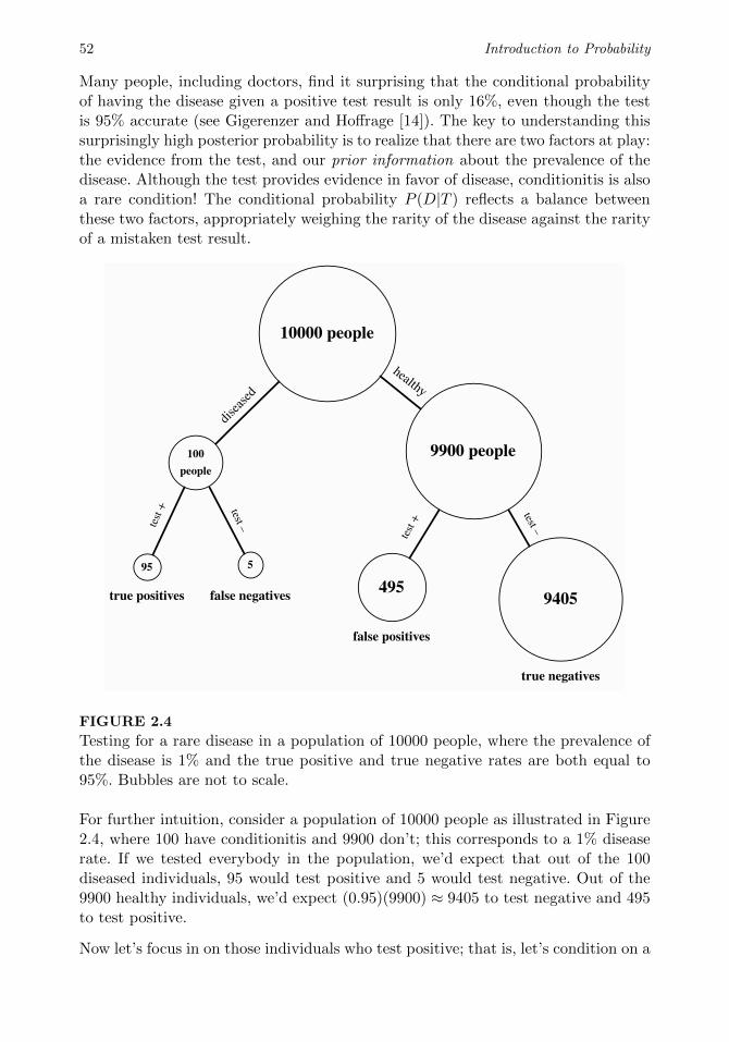
52 Introduction to Probability
Many people, including doctors, find it surprising that the conditional probabilityof having the disease given a positive test result is only 16%, even though the testis 95% accurate (see Gigerenzer and Ho↵rage [14]). The key to understanding thissurprisingly high posterior probability is to realize that there are two factors at play:the evidence from the test, and our prior information about the prevalence of thedisease. Although the test provides evidence in favor of disease, conditionitis is alsoa rare condition! The conditional probability P (D|T ) reflects a balance betweenthese two factors, appropriately weighing the rarity of the disease against the rarityof a mistaken test result.
10000 people
100 people
9900 peopledis
eased
healthy
595
test –
495 9405
test –
true positives false negatives
false positives
true negatives
test +
test +
FIGURE 2.4
Testing for a rare disease in a population of 10000 people, where the prevalence ofthe disease is 1% and the true positive and true negative rates are both equal to95%. Bubbles are not to scale.
For further intuition, consider a population of 10000 people as illustrated in Figure2.4, where 100 have conditionitis and 9900 don’t; this corresponds to a 1% diseaserate. If we tested everybody in the population, we’d expect that out of the 100diseased individuals, 95 would test positive and 5 would test negative. Out of the9900 healthy individuals, we’d expect (0.95)(9900) ⇡ 9405 to test negative and 495to test positive.
Now let’s focus in on those individuals who test positive; that is, let’s condition on a

Conditional probability 53
positive test result. The 95 true positives (i.e., the individuals who test positive andhave the disease) are far outnumbered by the 495 false positives (i.e., the individualswho test positive despite not having the disease). So most people who test positivefor the disease are actually disease-free! ⇤
2.4 Conditional probabilities are probabilities
When we condition on an event E, we update our beliefs to be consistent withthis knowledge, e↵ectively putting ourselves in a universe where we know that Eoccurred. Within our new universe, however, the laws of probability operate just asbefore. Conditional probability satisfies all the properties of probability! Therefore,any of the results we have derived about probability are still valid if we replace allunconditional probabilities with probabilities conditional on E. In particular:
• Conditional probabilities are between 0 and 1.
• P (S|E) = 1, P (;|E) = 0.
• If A1
, A2
, . . . are disjoint, then P ([1j=1
Aj |E) =P1
j=1
P (Aj |E).
• P (Ac|E) = 1� P (A|E).
• Inclusion-exclusion: P (A [B|E) = P (A|E) + P (B|E)� P (A \B|E).
h 2.4.1. When we write P (A|E), it does not mean that A|E is an event andwe’re taking its probability; A|E is not an event. Rather, P (·|E) is a probabilityfunction which assigns probabilities in accordance with the knowledge that E hasoccurred, and P (·) is a di↵erent probability function which assigns probabilitieswithout regard for whether E has occurred or not. When we take an event A andplug it into the P (·) function, we’ll get a number, P (A); when we plug it intothe P (·|E) function, we’ll get another number, P (A|E), which incorporates theinformation (if any) provided by knowing that E occurred.
To prove mathematically that conditional probabilities are probabilities, fix an eventE with P (E) > 0, and for any event A, define P (A) = P (A|E). This notation helpsemphasize the fact that we are fixing E and treating P (·|E) as our “new” probabilityfunction. We just need to check the two axioms of probability. First,
P (;) = P (;|E) =P (; \ E)
P (E)= 0, P (S) = P (S|E) =
P (S \ E)
P (E)= 1.
Second, if A1
, A2
, . . . are disjoint events, then
P (A1
[A2
[· · · ) = P ((A1
\ E) [ (A2
\ E) [ · · · )P (E)
=
P1j=1
P (Aj \ E)
P (E)=
1X
j=1
P (Aj |E).

54 Introduction to Probability
So P satisfies the axioms of probability.
Conversely, all probabilities can be thought of as conditional probabilities: wheneverwe make a probability statement, there is always some background information thatwe are conditioning on, even if we don’t state it explicitly. Consider the rain examplefrom the beginning of this chapter. It would be natural to base the initial probabilityof rain today, P (R), on the fraction of days in the past on which it rained. But whichdays in the past should we look at? If it’s November 1, should we only count pastrainy days in autumn, thus conditioning on the season? What about conditioning onthe exact month, or the exact day? We could ask the same about location: should welook at days when it rained in our exact location, or is it enough for it to have rainedsomewhere nearby? In order to determine the seemingly unconditional probabilityP (R), we actually have to make decisions about what background information tocondition on! These choices require careful thought and di↵erent people may comeup with di↵erent “prior” probabilities P (R) (though everyone can agree on how toupdate based on new evidence).
Since all probabilities are conditional on background information, we can imaginethat there is always a vertical conditioning bar, with background knowledgeK to theright of the vertical bar. Then the unconditional probability P (A) is just shorthandfor P (A|K); the background knowledge is absorbed into the letter P instead ofbeing written explicitly.
To summarize our discussion in a nutshell:
Conditional probabilities are probabilities, and all probabilities are conditional.
We now state conditional forms of Bayes’ rule and the law of total probability. Theseare obtained by taking the ordinary forms of Bayes’ rule and LOTP and adding Eto the right of the vertical bar everywhere.
Theorem 2.4.2 (Bayes’ rule with extra conditioning). Provided that P (A\E) > 0and P (B \ E) > 0, we have
P (A|B,E) =P (B|A,E)P (A|E)
P (B|E).
Theorem 2.4.3 (LOTP with extra conditioning). Let A1
, . . . , An be a partition ofS. Provided that P (Ai \ E) > 0 for all i, we have
P (B|E) =nX
i=1
P (B|Ai, E)P (Ai|E).
The extra conditioning forms of Bayes’ rule and LOTP can be proved similarly tohow we verified that P satisfies the axioms of probability, but they also follow di-rectly from the “metatheorem” that conditional probabilities are probabilities.
Example 2.4.4 (Random coin, continued). Continuing with the scenario fromExample 2.3.7, suppose that we have now seen our chosen coin land Heads three

Conditional probability 55
times. If we toss the coin a fourth time, what is the probability that it will landHeads once more?
Solution:
As before, let A be the event that the chosen coin lands Heads three times, anddefine a new event H for the chosen coin landing Heads on the fourth toss. Weare interested in P (H|A). It would be very helpful to know whether we have thefair coin. LOTP with extra conditioning gives us P (H|A) as a weighted average ofP (H|F,A) and P (H|F c, A), and within these two conditional probabilities we doknow whether we have the fair coin:
P (H|A) = P (H|F,A)P (F |A) + P (H|F c, A)P (F c|A)
=1
2· 0.23 + 3
4· (1� 0.23)
⇡ 0.69.
The posterior probabilities P (F |A) and P (F c|A) are from our answer to Example2.3.7.
An equivalent way to solve this problem is to define a new probability function Psuch that for any event B, P (B) = P (B|A). This new function assigns probabilitiesthat are updated with the knowledge that A occurred. Then by the ordinary law oftotal probability,
P (H) = P (H|F )P (F ) + P (H|F c)P (F c),
which is exactly the same as our use of LOTP with extra conditioning. This onceagain illustrates the principle that conditional probabilities are probabilities. ⇤We often want to condition on more than one piece of information, and we nowhave several ways of doing that. For example, here are some approaches for findingP (A|B,C):
1. We can think of B,C as the single event B\C and use the definition of conditionalprobability to get
P (A|B,C) =P (A,B,C)
P (B,C).
This is a natural approach if it’s easiest to think about B and C in tandem. Wecan then try to evaluate the numerator and denominator. For example, we can useLOTP in both the numerator and the denominator, or we can write the numeratoras P (B,C|A)P (A) (which would give us a version of Bayes’ rule) and use LOTP tohelp with the denominator.
2. We can use Bayes’ rule with extra conditioning on C to get
P (A|B,C) =P (B|A,C)P (A|C)
P (B|C).

56 Introduction to Probability
This is a natural approach if we want to think of everything in our problem as beingconditioned on C.
3. We can use Bayes’ rule with extra conditioning on B to get
P (A|B,C) =P (C|A,B)P (A|B)
P (C|B).
This is the same as the previous approach, except with the roles of B and C swapped.We mention it separately just to emphasize that it’s a bad idea to plug into a formulawithout thinking about which event should play which role.
It is both challenging and powerful that there are a variety of ways to approach thiskind of conditioning problem.
2.5 Independence of events
We have now seen several examples where conditioning on one event changes ourbeliefs about the probability of another event. The situation where events provideno information about each other is called independence.
Definition 2.5.1 (Independence of two events). Events A and B are independentif
P (A \B) = P (A)P (B).
If P (A) > 0 and P (B) > 0, then this is equivalent to
P (A|B) = P (A),
and also equivalent to P (B|A) = P (B).
In words, two events are independent if we can obtain the probability of theirintersection by multiplying their individual probabilities. Alternatively, A and Bare independent if learning that B occurred gives us no information that wouldchange our probabilities for A occurring (and vice versa).
Note that independence is a symmetric relation: if A is independent of B, then Bis independent of A.
h 2.5.2. Independence is completely di↵erent from disjointness. If A and B aredisjoint, then P (A\B) = 0, so disjoint events can be independent only if P (A) = 0or P (B) = 0. Knowing that A occurs tells us that B definitely did not occur, so Aclearly conveys information about B, meaning the two events are not independent(except if A or B already has zero probability).
Intuitively, it makes sense that if A provides no information about whether or notB occurred, then it also provides no information about whether or not Bc occurred.We now prove a handy result along those lines.
Conditional probability 57
Proposition 2.5.3. If A and B are independent, then A and Bc are independent,Ac and B are independent, and Ac and Bc are independent.
Proof. Let A and B be independent. Then
P (Bc|A) = 1� P (B|A) = 1� P (B) = P (Bc),
so A and Bc are independent. Swapping the roles of A and B, we have that Ac and Bare independent. Using the fact that A,B independent implies A,Bc independent,with Ac playing the role of A, we also have that Ac and Bc are independent. ⌅
We also often need to talk about independence of three or more events.
Definition 2.5.4 (Independence of three events). Events A, B, and C are said tobe independent if all of the following equations hold:
P (A \B) = P (A)P (B),
P (A \ C) = P (A)P (C),
P (B \ C) = P (B)P (C),
P (A \B \ C) = P (A)P (B)P (C).
If the first three conditions hold, we say that A, B, and C are pairwise independent.Pairwise independence does not imply independence: it is possible that just learningabout A or just learning about B is of no use in predicting whether C occurred,but learning that both A and B occurred could still be highly relevant for C. Hereis a simple example of this distinction.
Example 2.5.5 (Pairwise independence doesn’t imply independence). Considertwo fair, independent coin tosses, and let A be the event that the first is Heads,B the event that the second is Heads, and C the event that both tosses have thesame result. Then A, B, and C are pairwise independent but not independent, sinceP (A \ B \ C) = 1/4 while P (A)P (B)P (C) = 1/8. The point is that just knowingabout A or just knowing about B tells us nothing about C, but knowing whathappened with both A and B gives us information about C (in fact, in this case itgives us perfect information about C). ⇤On the other hand, P (A \ B \ C) = P (A)P (B)P (C) does not imply pairwiseindependence; this can be seen quickly by looking at the extreme case P (A) = 0,when the equation becomes 0 = 0 and tells us nothing about whether B and C areindependent.
We can define independence of any number of events similarly. Intuitively, the ideais that knowing what happened with any particular subset of the events gives us noinformation about what happened with the events not in that subset.
Definition 2.5.6 (Independence of many events). For n events A1
, A2
, . . . , An tobe independent, we require any pair to satisfy P (Ai\Aj) = P (Ai)P (Aj) (for i 6= j),

58 Introduction to Probability
any triplet to satisfy P (Ai \ Aj \ Ak) = P (Ai)P (Aj)P (Ak) (for i, j, k distinct),and similarly for all quadruplets, quintuplets, and so on. This can quickly becomeunwieldy, but later we will discuss other ways to think about independence. Forinfinitely many events, we say that they are independent if every finite subset of theevents is independent.
Conditional independence is defined analogously to independence.
Definition 2.5.7 (Conditional independence). Events A and B are said to beconditionally independent given E if P (A \B|E) = P (A|E)P (B|E).
h 2.5.8. It is easy to make terrible blunders stemming from confusing indepen-dence and conditional independence. Two events can be conditionally independentgiven E, but not independent. Two events can be independent, but not condition-ally independent given E. Two events can be conditionally independent given E,but not independent given Ec. The next few examples illustrate these distinctions.Great care is needed in working with conditional probabilities and conditional in-dependence!
Example 2.5.9 (Conditional independence doesn’t imply independence). Return-ing once more to the scenario from Example 2.3.7, suppose we have chosen either afair coin or a biased coin with probability 3/4 of heads, but we do not know whichone we have chosen. We flip the coin a number of times. Conditional on choosing thefair coin, the coin tosses are independent, with each toss having probability 1/2 ofheads. Similarly, conditional on choosing the biased coin, the tosses are independent,each with probability 3/4 of heads.
However, the coin tosses are not unconditionally independent, because if we don’tknow which coin we’ve chosen, then observing the sequence of tosses gives us infor-mation about whether we have the fair coin or the biased coin in our hand. This inturn helps us to predict the outcomes of future tosses from the same coin.
To state this formally, let F be the event that we’ve chosen the fair coin, and let A1
and A2
be the events that the first and second coin tosses land heads. Conditional onF , A
1
and A2
are independent, but A1
and A2
are not unconditionally independentbecause A
1
provides information about A2
. ⇤Example 2.5.10 (Independence doesn’t imply conditional independence). Supposethat my friends Alice and Bob are the only two people who ever call me. Each day,they decide independently whether to call me: letting A be the event that Alicecalls and B be the event that Bob calls, A and B are unconditionally independent.But suppose that I hear the phone ringing now. Conditional on this observation,A and B are no longer independent: if the phone call isn’t from Alice, it must befrom Bob. In other words, letting R be the event that the phone is ringing, we haveP (B|R) < 1 = P (B|Ac, R), so B and Ac are not conditionally independent givenR, and likewise for A and B. ⇤Example 2.5.11 (Conditional independence given E vs. given Ec). Suppose thereare two types of classes: good classes and bad classes. In good classes, if you work
Conditional probability 59
hard, you are very likely to get an A. In bad classes, the professor randomly assignsgrades to students regardless of their e↵ort. Let G be the event that a class is good,W be the event that you work hard, and A be the event that you receive an A. ThenW and A are conditionally independent given Gc, but they are not conditionallyindependent given G! ⇤
2.6 Coherency of Bayes’ rule
An important property of Bayes’ rule is that it is coherent : if we receive multiplepieces of information and wish to update our probabilities to incorporate all theinformation, it does not matter whether we update sequentially, taking each pieceof evidence into account one at a time, or simultaneously, using all the evidenceat once. Suppose, for example, that we’re conducting a weeklong experiment thatyields data at the end of each day. We could use Bayes’ rule every day to updateour probabilities based on the data from that day. Or we could go on vacation forthe week, come back on Friday afternoon, and update using the entire week’s worthof data. Either method will give the same result.
Let’s look at a concrete application of this principle.
Example 2.6.1 (Testing for a rare disease, continued). Fred, who tested positivefor conditionitis in Example 2.3.9, decides to get tested a second time. The newtest is independent of the original test (given his disease status) and has the samesensitivity and specificity. Unfortunately for Fred, he tests positive a second time.Find the probability that Fred has the disease, given the evidence, in two ways: inone step, conditioning on both test results simultaneously, and in two steps, firstupdating the probabilities based on the first test result, and then updating againbased on the second test result.
Solution:
Let D be the event that he has the disease, T1
that the first test result is positive,and T
2
that the second test result is positive. In Example 2.3.9, we used Bayes’ ruleand the law of total probability to find P (D|T
1
). Another quick solution uses theodds form of Bayes’ rule:
P (D|T1
)
P (Dc|T1
)=
P (D)
P (Dc)
P (T1
|D)
P (T1
|Dc)=
1
99· 0.950.05
⇡ 0.19.
Since P (D|T1
)/(1 � P (D|T1
)) = 0.19, we have P (D|T1
) = 0.19/(1 + 0.19) ⇡ 0.16,in agreement with our answer from before. The odds form of Bayes’ rule is fasterin this case because we don’t need to compute the unconditional probability P (T
1
)in the denominator of the ordinary Bayes’ rule. Now, again using the odds form ofBayes’ rule, let’s find out what happens if Fred tests positive a second time.

60 Introduction to Probability
One-step method : Updating based on both test results at once, we have
P (D|T1
\ T2
)
P (Dc|T1
\ T2
)=
P (D)
P (Dc)
P (T1
\ T2
|D)
P (T1
\ T2
|Dc)
=1
99· 0.95
2
0.052=
361
99⇡ 3.646,
which corresponds to a probability of 0.78.
Two-step method : After the first test, the posterior odds of Fred having the diseaseare
P (D|T1
)
P (Dc|T1
)=
1
99· 0.950.05
⇡ 0.19,
from the above. These posterior odds become the new prior odds, and then updatingbased on the second test gives
P (D|T1
\ T2
)
P (Dc|T1
\ T2
)=
P (D|T1
)
P (Dc|T1
)
P (T2
|D,T1
)
P (T2
|Dc, T1
)
=
✓1
99· 0.950.05
◆0.95
0.05=
361
99⇡ 3.646,
which is the same result as above.
Note that with a second positive test result, the probability that Fred has the diseasejumps from 0.16 to 0.78, making us much more confident that Fred is actuallya✏icted with conditionitis. The moral of the story is that getting a second opinionis a good idea! ⇤
2.7 Conditioning as a problem-solving tool
Conditioning is a powerful tool for solving problems because it lets us engage inwishful thinking : when we encounter a problem that would be made easier if onlywe knew whether E happened or not, we can condition on E and then on Ec,consider these possibilities separately, then combine them using LOTP.
2.7.1 Strategy: condition on what you wish you knew
Example 2.7.1 (Monty Hall). On the game show Let’s Make a Deal, hosted byMonty Hall, a contestant chooses one of three closed doors, two of which have a goatbehind them and one of which has a car. Monty, who knows where the car is, thenopens one of the two remaining doors. The door he opens always has a goat behindit (he never reveals the car!). If he has a choice, then he picks a door at random

Conditional probability 61
with equal probabilities. Monty then o↵ers the contestant the option of switchingto the other unopened door. If the contestant’s goal is to get the car, should sheswitch doors?
1 2 3
Solution:
Let’s label the doors 1 through 3. Without loss of generality, we can assume thecontestant picked door 1 (if she didn’t pick door 1, we could simply relabel thedoors, or rewrite this solution with the door numbers permuted). Monty opensa door, revealing a goat. As the contestant decides whether or not to switch tothe remaining unopened door, what does she really wish she knew? Naturally, herdecision would be a lot easier if she knew where the car was! This suggests thatwe should condition on the location of the car. Let Ci be the event that the car isbehind door i, for i = 1, 2, 3. By the law of total probability,
P (get car) = P (get car|C1
) · 13+ P (get car|C
2
) · 13+ P (get car|C
3
) · 13.
Suppose the contestant employs the switching strategy. If the car is behind door 1,then switching will fail, so P (get car|C
1
) = 0. If the car is behind door 2 or 3, thenbecause Monty always reveals a goat, the remaining unopened door must containthe car, so switching will succeed. Thus,
P (get car) = 0 · 13+ 1 · 1
3+ 1 · 1
3=
2
3,
so the switching strategy succeeds 2/3 of the time. The contestant should switch tothe other door.
Figure 2.5 is a tree diagram of the argument we have just outlined: using the switch-ing strategy, the contestant will win as long as the car is behind doors 2 or 3, whichhas probability 2/3. We can also give an intuitive frequentist argument in favor ofswitching. Imagine playing this game 1000 times. Typically, about 333 times yourinitial guess for the car’s location will be correct, in which case switching will fail.The other 667 or so times, you will win by switching.
There’s a subtlety though, which is that when the contestant chooses whether toswitch, she also knows which door Monty opened. We showed that the unconditionalprobability of success is 2/3 (when following the switching strategy), but let’s alsoshow that the conditional probability of success for switching, given the informationthat Monty provides, is also 2/3.

62 Introduction to Probability
door 1
door 1
door 2
door 3
door 2 door 3
door 3 door 2
You choose:
Car is behind:
Monty opens:
Outcome if you switch:
1/3
1/3
1/3
1/2
1/2
1
1
1/6
1/6
1/3
1/3
FIGURE 2.5
Tree diagram of Monty Hall problem. Switching gets the car 2/3 of the time.
Let Mj be the event that Monty opens door j, for j = 2, 3. Then
P (get car) = P (get car|M2
)P (M2
) + P (get car|M3
)P (M3
),
where by symmetry P (M2
) = P (M3
) = 1/2 and P (get car|M2
) = P (get car|M3
).The symmetry here is that there is nothing in the statement of the problem thatdistinguishes between door 2 and door 3; in contrast, Problem 39 considers a scenariowhere Monty enjoys opening door 2 more than he enjoys opening door 3.
Let x = P (get car|M2
) = P (get car|M3
). Plugging in what we know,
2
3= P (get car) =
x
2+
x
2= x,
as claimed.
Bayes’ rule also works nicely for finding the conditional probability of success usingthe switching strategy, given the evidence. Suppose that Monty opens door 2. Usingthe notation and results above,
P (C1
|M2
) =P (M
2
|C1
)P (C1
)
P (M2
)=
(1/2)(1/3)
1/2=
1
3.
So given that Monty opens door 2, there is a 1/3 chance that the contestant’soriginal choice of door has the car, which means that there is a 2/3 chance that theswitching strategy will succeed.
Many people, upon seeing this problem for the first time, argue that there is noadvantage to switching: “There are two doors remaining, and one of them hasthe car, so the chances are 50-50.” After the last chapter, we recognize that this

Conditional probability 63
argument misapplies the naive definition of probability. Yet the naive definition,even when inappropriate, has a powerful hold on people’s intuitions. When Marilynvos Savant presented a correct solution to the Monty Hall problem in her columnfor Parade magazine in 1990, she received thousands upon thousands of letters fromreaders (even mathematicians) insisting that she was wrong.
To build correct intuition, let’s consider an extreme case. Suppose that there area million doors, 999,999 of which contain goats and 1 of which has a car. Afterthe contestant’s initial pick, Monty opens 999,998 doors with goats behind themand o↵ers the choice to switch. In this extreme case, it becomes clear that theprobabilities are not 50-50 for the two unopened doors; very few people wouldstubbornly stick with their original choice. The same is true for the three-door case.
Just as we had to make assumptions about how we came across the random girl inExample 2.2.6, here the 2/3 success rate of the switching strategy depends on theassumptions we make about how Monty decides which door to open. In the exercises,we consider several variants and generalizations of the Monty Hall problem, someof which change the desirability of the switching strategy. ⇤
2.7.2 Strategy: condition on the first step
In problems with a recursive structure, it can often be useful to condition on thefirst step of the experiment. The next two examples apply this strategy, which wecall first-step analysis.
Example 2.7.2 (Branching process). A single amoeba, Bobo, lives in a pond. Afterone minute Bobo will either die, split into two amoebas, or stay the same, with equalprobability, and in subsequent minutes all living amoebas will behave the same way,independently. What is the probability that the amoeba population will eventuallydie out?
... ... ...
1/3 1/31/3
Solution:
Let D be the event that the population eventually dies out; we want to find P (D).We proceed by conditioning on the outcome at the first step: let Bi be the event
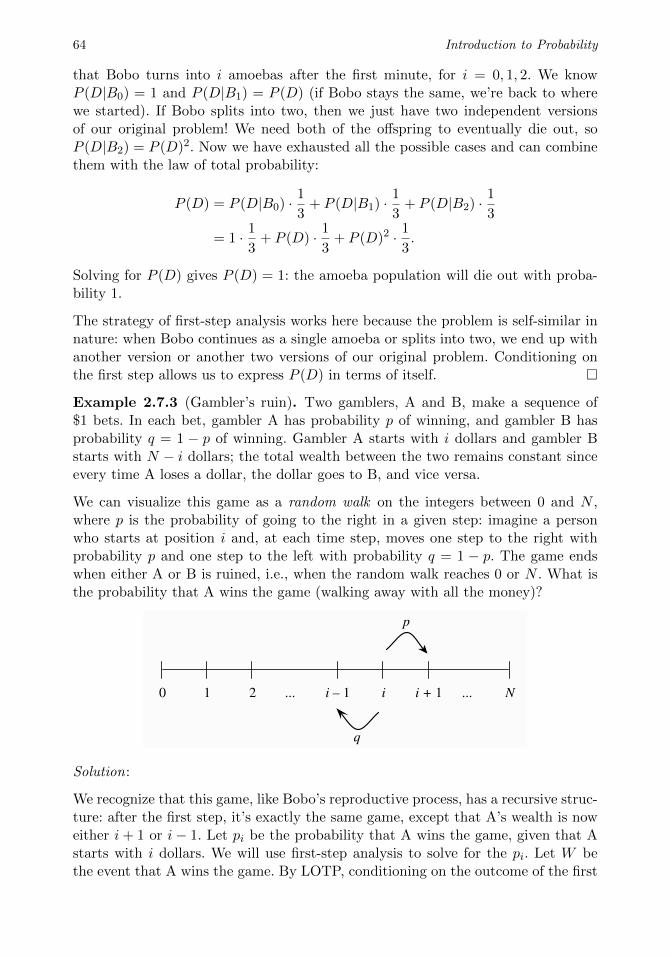
64 Introduction to Probability
that Bobo turns into i amoebas after the first minute, for i = 0, 1, 2. We knowP (D|B
0
) = 1 and P (D|B1
) = P (D) (if Bobo stays the same, we’re back to wherewe started). If Bobo splits into two, then we just have two independent versionsof our original problem! We need both of the o↵spring to eventually die out, soP (D|B
2
) = P (D)2. Now we have exhausted all the possible cases and can combinethem with the law of total probability:
P (D) = P (D|B0
) · 13+ P (D|B
1
) · 13+ P (D|B
2
) · 13
= 1 · 13+ P (D) · 1
3+ P (D)2 · 1
3.
Solving for P (D) gives P (D) = 1: the amoeba population will die out with proba-bility 1.
The strategy of first-step analysis works here because the problem is self-similar innature: when Bobo continues as a single amoeba or splits into two, we end up withanother version or another two versions of our original problem. Conditioning onthe first step allows us to express P (D) in terms of itself. ⇤Example 2.7.3 (Gambler’s ruin). Two gamblers, A and B, make a sequence of$1 bets. In each bet, gambler A has probability p of winning, and gambler B hasprobability q = 1 � p of winning. Gambler A starts with i dollars and gambler Bstarts with N � i dollars; the total wealth between the two remains constant sinceevery time A loses a dollar, the dollar goes to B, and vice versa.
We can visualize this game as a random walk on the integers between 0 and N ,where p is the probability of going to the right in a given step: imagine a personwho starts at position i and, at each time step, moves one step to the right withprobability p and one step to the left with probability q = 1 � p. The game endswhen either A or B is ruined, i.e., when the random walk reaches 0 or N . What isthe probability that A wins the game (walking away with all the money)?
i ...i + 1 Ni – 1...1 20
q
p
Solution:
We recognize that this game, like Bobo’s reproductive process, has a recursive struc-ture: after the first step, it’s exactly the same game, except that A’s wealth is noweither i+ 1 or i� 1. Let pi be the probability that A wins the game, given that Astarts with i dollars. We will use first-step analysis to solve for the pi. Let W bethe event that A wins the game. By LOTP, conditioning on the outcome of the first

Conditional probability 65
round, we have
pi = P (W |A starts at i, wins round 1) · p+ P (W |A starts at i, loses round 1) · q= P (W |A starts at i+ 1) · p+ P (W |A starts at i� 1) · q= pi+1
· p+ pi�1
· q.
This must be true for all i from 1 to N�1, and we also have the boundary conditionsp0
= 0 and pN = 1. Now we can solve this equation, called a di↵erence equation, toobtain the pi. Section A.4 of the math appendix discusses how to solve di↵erenceequations, so we will omit some of the steps here.
The characteristic polynomial of the di↵erence equation is px2 � x + q = 0, whichhas roots of 1 and q/p. If p 6= 1/2, these roots are distinct, and the general solutionis
pi = a · 1i + b ·✓q
p
◆i
.
Using the boundary conditions p0
= 0 and pN = 1, we get
a = �b =1
1�⇣qp
⌘N ,
and we simply plug these back in to get the specific solution. If p = 1/2, the rootsof the characteristic polynomial are not distinct, so the general solution is
pi = a · 1i + b · i · 1i.
The boundary conditions give a = 0 and b = 1/N .
In summary, the probability of A winning with a starting wealth of i is
pi =
8><
>:
1�⇣
q
p
⌘i
1�⇣
q
p
⌘N
if p 6= 1/2,
iN if p = 1/2.
The p = 1/2 case is consistent with the p 6= 1/2 case, in the sense that
limp! 1
2
1� ( qp)i
1� ( qp)N
=i
N.
To see this, let x = q/p and let x approach 1. By L’Hopital’s rule,
limx!1
1� xi
1� xN= lim
x!1
ixi�1
NxN�1
=i
N.
By symmetry, the probability of B winning from a starting wealth ofN�i is obtainedby switching the roles of q and p, and of i and N � i. It can then be verified thatfor all i and all p, P (A wins) + P (B wins) = 1, so the game is guaranteed to end:neverending oscillation has probability 0. ⇤

66 Introduction to Probability
2.8 Pitfalls and paradoxes
The next two examples are fallacies of conditional thinking that have arisen in thelegal context. The prosecutor’s fallacy is the confusion of P (A|B) with P (B|A); thedefense attorney’s fallacy is the failure to condition on all the evidence.
h 2.8.1 (Prosecutor’s fallacy). In 1998, Sally Clark was tried for murder aftertwo of her sons died shortly after birth. During the trial, an expert witness forthe prosecution testified that the probability of a newborn dying of sudden infantdeath syndrome (SIDS) was 1/8500, so the probability of two deaths due to SIDSin one family was (1/8500)2, or about one in 73 million. Therefore, he continued,the probability of Clark’s innocence was one in 73 million.
There are at least two major problems with this line of reasoning. First, the expertwitness found the probability of the intersection of “first son dies of SIDS” and“second son dies of SIDS” by multiplying the individual event probabilities; as weknow, this is only valid if deaths due to SIDS are independent within a family. Thisindependence would not hold if genetic or other family-specific risk factors cause allnewborns within certain families to be at increased risk of SIDS.
Second, the so-called expert has confused two di↵erent conditional probabilities:P (innocence|evidence) is di↵erent from P (evidence|innocence). The witness claimsthat the probability of observing two newborn deaths if the defendant were innocentis extremely low; that is, P (evidence|innocence) is small. What we are interested in,however, is P (innocence|evidence), the probability that the defendant is innocentgiven all the evidence. By Bayes’ rule,
P (innocence|evidence) = P (evidence|innocence)P (innocence)
P (evidence),
so to calculate the conditional probability of innocence given the evidence, we musttake into account P (innocence), the prior probability of innocence. This probabilityis extremely high: although double deaths due to SIDS are rare, so are doubleinfanticides! The posterior probability of innocence given the evidence is a balancebetween P (evidence|innocence), which is low, and P (innocence), which is high. Theexpert’s probability of (1/8500)2, questionable in and of itself, is only part of theequation.
Sadly, Clark was convicted of murder and sent to prison, partly based on the expert’swrongheaded testimony, and spent over three years in jail before her conviction wasoverturned. The outcry over the misuse of conditional probability in the Sally Clarkcase led to the review of hundreds of other cases where similar faulty logic was usedby the prosecution.
h 2.8.2 (Defense attorney’s fallacy). A woman has been murdered, and her husbandis put on trial for this crime. Evidence comes to light that the defendant had a history

Conditional probability 67
of abusing his wife. The defense attorney argues that the evidence of abuse shouldbe excluded on grounds of irrelevance, since only 1 in 10,000 men who abuse theirwives subsequently murder them. Should the judge grant the defense attorney’smotion to bar this evidence from trial?
Suppose that the defense attorney’s 1-in-10,000 figure is correct, and further assumethe following facts: 1 in 10 men commit abuse against their wives, 1 in 5 marriedwomen who are murdered are murdered by their husbands, and 50% of husbandswho murder their wives previously abused them.
Let A be the event that the husband commits abuse against his wife, and letG be theevent that the husband is guilty. The defense’s argument is that P (G|A) = 1/10,000,so guilt is still extremely unlikely conditional on a previous history of abuse.
However, the defense attorney fails to condition on a crucial fact: in this case, weknow that the wife was murdered. Therefore, the relevant probability is not P (G|A),but P (G|A,M), where M is the event that the wife was murdered.
Bayes’ rule with extra conditioning gives
P (G|A,M) =P (A|G,M)P (G|M)
P (A|G,M)P (G|M) + P (A|Gc,M)P (Gc|M)
=0.5 · 0.2
0.5 · 0.2 + 0.1 · 0.8
=5
9.
The evidence of abuse has increased the probability of guilt from 20% to over 50%, sothe defendant’s history of abuse gives important information about his probabilityof guilt, contrary to the defense attorney’s argument.
Note that in the above calculation, we did not use the defense attorney’s P (G|A)number anywhere; it is irrelevant to our calculation because it does not account forthe fact that the wife was murdered. We must condition on all the evidence.
We end this chapter with a paradox about conditional probability and aggregationof data.
Example 2.8.3 (Simpson’s paradox). Two doctors, Dr. Hibbert and Dr. Nick, eachperform two types of surgeries: heart surgery and Band-Aid removal. Each surgerycan be either a success or a failure. The two doctors’ respective records are given inthe following tables, and shown graphically in Figure 2.6, where white dots representsuccessful surgeries and black dots represent failed surgeries.
Heart Band-Aid
Success 70 10Failure 20 0
Dr. Hibbert
Heart Band-Aid
Success 2 81Failure 8 9
Dr. Nick

68 Introduction to Probability
Dr. Hibbert had a higher success rate than Dr. Nick in heart surgeries: 70 out of 90versus 2 out of 10. Dr. Hibbert also had a higher success rate in Band-Aid removal:10 out of 10 versus 81 out of 90. But if we aggregate across the two types of surgeriesto compare overall surgery success rates, Dr. Hibbert was successful in 80 out of100 surgeries while Dr. Nick was successful in 83 out of 100 surgeries: Dr. Nick’soverall success rate is higher!
Dr. Hibbert Dr. Nick
heart
band-aid
FIGURE 2.6
An example of Simpson’s paradox. White dots represent successful surgeries andblack dots represent failed surgeries. Dr. Hibbert is better in both types of surgerybut has a lower overall success rate, because he is performing the harder type ofsurgery much more often than Dr. Nick is.
What’s happening is that Dr. Hibbert, presumably due to his reputation as thesuperior doctor, is performing a greater number of heart surgeries, which are inher-ently riskier than Band-Aid removals. His overall success rate is lower not becauseof lesser skill on any particular type of surgery, but because a larger fraction of hissurgeries are risky.
Let’s use event notation to make this precise. For events A, B, and C, we say thatwe have a Simpson’s paradox if
P (A|B,C) < P (A|Bc, C)
P (A|B,Cc) < P (A|Bc, Cc),
butP (A|B) > P (A|Bc).
In this case, let A be the event of a successful surgery, B be the event that Dr. Nickis the surgeon, and C be the event that the surgery is a heart surgery. The conditionsfor Simpson’s paradox are fulfilled because the probability of a successful surgery

Conditional probability 69
is lower under Dr. Nick than under Dr. Hibbert whether we condition on heartsurgery or on Band-Aid removal, but the overall probability of success is higher forDr. Nick.
The law of total probability tells us mathematically why this can happen:
P (A|B) = P (A|C,B)P (C|B) + P (A|Cc, B)P (Cc|B)
P (A|Bc) = P (A|C,Bc)P (C|Bc) + P (A|Cc, Bc)P (Cc|Bc).
Although we haveP (A|C,B) < P (A|C,Bc)
andP (A|Cc, B) < P (A|Cc, Bc),
the weights P (C|B) and P (Cc|B) can flip the overall balance. In our situation
P (Cc|B) > P (Cc|Bc),
since Dr. Nick is much more likely to be performing Band-Aid removals, and thisdi↵erence is large enough to cause P (A|B) to be greater than P (A|Bc).
Aggregation across di↵erent types of surgeries presents a misleading picture of thedoctors’ abilities because we lose the information about which doctor tends to per-form which type of surgery. When we think confounding variables like surgery typecould be at play, we should examine the disaggregated data to see what is reallygoing on.
Simpson’s paradox arises in many real-world contexts. In the following examples,you should try to identify the events A, B, and C that create the paradox.
• Gender discrimination in college admissions: In the 1970s, men were significantlymore likely than women to be admitted for graduate study at the University ofCalifornia, Berkeley, leading to charges of gender discrimination. Yet within mostindividual departments, women were admitted at a higher rate than men. It wasfound that women tended to apply to the departments with more competitiveadmissions, while men tended to apply to less competitive departments.
• Baseball batting averages : It is possible for player 1 to have a higher batting averagethan player 2 in the first half of a baseball season and a higher batting averagethan player 2 in the second half of the season, yet have a lower overall battingaverage for the entire season. It depends on how many at-bats the players havein each half of the season. (An at-bat is when it’s a player’s turn to try to hit theball; the player’s batting average is the number of hits the player gets divided bythe player’s number of at-bats.)
• Health e↵ects of smoking : Cochran [5] found that within any age group, cigarettesmokers had higher mortality rates than cigar smokers, but because cigarette smok-ers were on average younger than cigar smokers, overall mortality rates were lowerfor cigarette smokers.

70 Introduction to Probability
⇤
2.9 Recap
The conditional probability of A given B is
P (A|B) =P (A \B)
P (B).
Conditional probability has exactly the same properties as probability, but P (·|B)updates our uncertainty about events to reflect the observed evidence B. Eventswhose probabilities are unchanged after observing the evidence B are said to beindependent of B. Two events can also be conditionally independent given a thirdevent E. Conditional independence does not imply unconditional independence, nordoes unconditional independence imply conditional independence.
Two important results about conditional probability are Bayes’ rule, which relatesP (A|B) to P (B|A), and the law of total probability, which allows us to get uncon-ditional probabilities by partitioning the sample space and calculating conditionalprobabilities within each slice of the partition.
Conditioning is extremely helpful for problem-solving because it allows us to break aproblem into smaller pieces, consider all possible cases separately, and then combinethem. When using this strategy, we should try to condition on the information that,if known, would make the problem simpler, hence the saying condition on whatyou wish you knew. When a problem involves multiple stages, it can be helpful tocondition on the first step to obtain a recursive relationship.
Common mistakes in thinking conditionally include:
• confusion of the prior probability P (A) with the posterior probability P (A|B);
• the prosecutor’s fallacy, confusing P (A|B) with P (B|A);
• the defense attorney’s fallacy, failing to condition on all the evidence;
• unawareness of Simpson’s paradox and the importance of thinking carefully aboutwhether to aggregate data.
Figure 2.7 illustrates how probabilities can be updated as new evidence comes insequentially. Imagine that there is some event A that we are interested in. OnMonday morning, for example, our prior probability for A is P (A). If we observe onMonday afternoon that B occurred, then we can use Bayes’ rule (or the definitionof conditional probability) to compute the posterior probability P (A|B).
We use this posterior probability for A as the new prior on Tuesday morning, andthen we continue to collect evidence. Suppose that on Tuesday we observe that C

Conditional probability 71
events
Monday
P (A)(Monday’s prior for A)
P (A|B) =P (A,B)
P (B)=
P (B|A)P (A)
P (B)(Monday’s posterior for A)
Tuesday
We already knowthat B occurred.We learn on Tuesdaythat C occurred.
P (A|B,C) =P (A,B,C)
P (B,C)
=P (C|A,B)P (A|B)
P (C|B)
P (A|B)(Tuesday’s prior for A)
(Tuesday’s posterior for A)
A,B,C
A,B,C
We learn on Mondaythat B occurred.
What can happen?
events
What can happen?
numbers
numbers
P
P
FIGURE 2.7
Conditional probability tells us how to update probabilities as new evidence comesin. Shown are the probabilities for an event A initially, after obtaining one piece ofevidence B, and after obtaining a second piece of evidence C. The posterior for Aafter observing the first piece of evidence becomes the new prior before observingthe second piece of evidence. After both B and C are observed, a new posterior forA can be found in various ways. This then becomes the new prior if more evidencewill be collected.
72 Introduction to Probability
occurred. Then we can compute the new posterior probability P (A|B,C) in variousways (in this context, probably the most natural way is to use Bayes’ rule withextra conditioning on B). This in turn becomes the new prior if we are going tocontinue to collect evidence.
2.10 R
Simulating the frequentist interpretation
Recall that the frequentist interpretation of conditional probability based on a largenumber n of repetitions of an experiment is P (A|B) ⇡ nAB/nB, where nAB is thenumber of times that A \ B occurs and nB is the number of times that B occurs.Let’s try this out by simulation, and verify the results of Example 2.2.5. So let’ssimulate n families, each with two children.
n <- 10^5
child1 <- sample(2,n,replace=TRUE)
child2 <- sample(2,n,replace=TRUE)
Here child1 is a vector of length n, where each element is a 1 or a 2. Letting 1 standfor “girl” and 2 stand for “boy”, this vector represents the gender of the elder childin each of the n families. Similarly, child2 represents the gender of the youngerchild in each family.
Alternatively, we could have used
sample(c("girl","boy"),n,replace=TRUE)
but it is more convenient working with numerical values.
Let A be the event that both children are girls and B the event that the elder is a girl.Following the frequentist interpretation, we count the number of repetitions whereB occurred and name it n.b, and we also count the number of repetitions whereA \ B occurred and name it n.ab. Finally, we divide n.ab by n.b to approximateP (A|B).
n.b <- sum(child1==1)
n.ab <- sum(child1==1 & child2==1)
n.ab/n.b
The ampersand & is an elementwise AND, so n.ab is the number of families whereboth the first child and the second child are girls. When we ran this code, we got0.50, confirming our answer P (both girls|elder is a girl) = 1/2.
Now let A be the event that both children are girls and B the event that at leastone of the children is a girl. Then A \ B is the same, but n.b needs to count the

Conditional probability 73
number of families where at least one child is a girl. This is accomplished with theelementwise OR operator | (this is not a conditioning bar; it is an inclusive OR,returning TRUE if at least one element is TRUE).
n.b <- sum(child1==1 | child2==1)
n.ab <- sum(child1==1 & child2==1)
n.ab/n.b
For us, the result was 0.33, confirming that P (both girls|at least one girl) =1/3.
Monty Hall simulation
Many long, bitter debates about the Monty Hall problem could have been avertedby trying it out with a simulation. To study how well the never-switch strategy per-forms, let’s generate 105 runs of the Monty Hall game. To simplify notation, assumethe contestant always chooses door 1. Then we can generate a vector specifyingwhich door has the car for each repetition:
n <- 10^5
cardoor <- sample(3,n,replace=TRUE)
At this point we could generate the vector specifying which doors Monty opens,but that’s unnecessary since the never-switch strategy succeeds if and only if door1 has the car! So the fraction of times when the never-switch strategy succeedsis sum(cardoor==1)/n, which was 0.334 in our simulation. This is very close to1/3.
What if we want to play the Monty Hall game interactively? We can do this byprogramming a function. Entering the following code in R defines a function calledmonty, which can then be invoked by entering the command monty() any time youfeel like playing the game!
monty <- function() {
doors <- 1:3
# randomly pick where the car is
cardoor <- sample(doors,1)
# prompt player
print("Monty Hall says ‘Pick a door, any door!’")
# receive the player’s choice of door (should be 1,2, or 3)
chosen <- scan(what = integer(), nlines = 1, quiet = TRUE)
# pick Monty’s door (can’t be the player’s door or the car door)
if (chosen != cardoor) montydoor <- doors[-c(chosen, cardoor)]

74 Introduction to Probability
else montydoor <- sample(doors[-chosen],1)
# find out whether the player wants to switch doors
print(paste("Monty opens door ", montydoor, "!", sep=""))
print("Would you like to switch (y/n)?")
reply <- scan(what = character(), nlines = 1, quiet = TRUE)
# interpret what player wrote as "yes" if it starts with "y"
if (substr(reply,1,1) == "y") chosen <- doors[-c(chosen,montydoor)]
# announce the result of the game!
if (chosen == cardoor) print("You won!")
else print("You lost!")
}
The print command prints its argument to the screen. We combine this with paste
since print("Monty opens door montydoor") would literally print “Monty opensdoor montydoor”. The scan command interactively requests input from the user;we use what = integer() when we want the user to enter an integer and what
= character() when we want the user to enter text. Using substr(reply,1,1)
extracts the first character of reply, in case the user replies with “yes” or “yep” or“yeah!” rather than with “y”.
2.11 Exercises
Conditioning on evidence
1. s� A spam filter is designed by looking at commonly occurring phrases in spam. Supposethat 80% of email is spam. In 10% of the spam emails, the phrase “free money” is used,whereas this phrase is only used in 1% of non-spam emails. A new email has just arrived,which does mention “free money”. What is the probability that it is spam?
2. s� A woman is pregnant with twin boys. Twins may be either identical or fraternal (non-identical). In general, 1/3 of twins born are identical. Obviously, identical twins mustbe of the same sex; fraternal twins may or may not be. Assume that identical twins areequally likely to be both boys or both girls, while for fraternal twins all possibilities areequally likely. Given the above information, what is the probability that the woman’stwins are identical?
3. According to the CDC (Centers for Disease Control and Prevention), men who smoke are23 times more likely to develop lung cancer than men who don’t smoke. Also accordingto the CDC, 21.6% of men in the U.S. smoke. What is the probability that a man inthe U.S. is a smoker, given that he develops lung cancer?
4. Fred is answering a multiple-choice problem on an exam, and has to choose one of noptions (exactly one of which is correct). Let K be the event that he knows the answer,and R be the event that he gets the problem right (either through knowledge or through

Conditional probability 75
luck). Suppose that if he knows the right answer he will definitely get the problem right,but if he does not know then he will guess completely randomly. Let P (K) = p.
(a) Find P (K|R) (in terms of p and n).
(b) Show that P (K|R) � p, and explain why this makes sense intuitively. When (if ever)does P (K|R) equal p?
5. Three cards are dealt from a standard, well-shu✏ed, deck. The first two cards are flippedover, revealing the Ace of Spades as the first card and the 8 of Clubs as the second card.Given this information, find the probability that the third card is an ace in two ways:using the definition of conditional probability, and by symmetry.
6. A hat contains 100 coins, where 99 are fair but one is double-headed (always landingHeads). A coin is chosen uniformly at random. The chosen coin is flipped 7 times, and itlands Heads all 7 times. Given this information, what is the probability that the chosencoin is double-headed? (Of course, another approach here would be to look at both sidesof the coin—but this is a metaphorical coin.)
7. A hat contains 100 coins, where at least 99 are fair, but there may be one that is double-headed (always landing Heads); if there is no such coin, then all 100 are fair. Let D bethe event that there is such a coin, and suppose that P (D) = 1/2. A coin is chosenuniformly at random. The chosen coin is flipped 7 times, and it lands Heads all 7 times.
(a) Given this information, what is the probability that one of the coins is double-headed?
(b) Given this information, what is the probability that the chosen coin is double-headed?
8. The screens used for a certain type of cell phone are manufactured by 3 companies,A, B, and C. The proportions of screens supplied by A, B, and C are 0.5, 0.3, and0.2, respectively, and their screens are defective with probabilities 0.01, 0.02, and 0.03,respectively. Given that the screen on such a phone is defective, what is the probabilitythat Company A manufactured it?
9. (a) Show that if events A1
and A2
have the same prior probability P (A1
) = P (A2
),A
1
implies B, and A2
implies B, then A1
and A2
have the same posterior probabilityP (A
1
|B) = P (A2
|B) if it is observed that B occurred.
(b) Explain why (a) makes sense intuitively, and give a concrete example.
10. Fred is working on a major project. In planning the project, two milestones are set up,with dates by which they should be accomplished. This serves as a way to track Fred’sprogress. Let A
1
be the event that Fred completes the first milestone on time, A2
bethe event that he completes the second milestone on time, and A
3
be the event that hecompletes the project on time.
Suppose that P (Aj+1
|Aj) = 0.8 but P (Aj+1
|Acj) = 0.3 for j = 1, 2, since if Fred falls
behind on his schedule it will be hard for him to get caught up. Also, assume that thesecond milestone supersedes the first, in the sense that once we know whether he ison time in completing the second milestone, it no longer matters what happened withthe first milestone. We can express this by saying that A
1
and A3
are conditionallyindependent given A
2
and they’re also conditionally independent given Ac2
.
(a) Find the probability that Fred will finish the project on time, given that he completesthe first milestone on time. Also find the probability that Fred will finish the project ontime, given that he is late for the first milestone.
(b) Suppose that P (A1
) = 0.75. Find the probability that Fred will finish the projecton time.
11. An exit poll in an election is a survey taken of voters just after they have voted. Onemajor use of exit polls has been so that news organizations can try to figure out as

76 Introduction to Probability
soon as possible who won the election, before the votes are o�cially counted. This hasbeen notoriously inaccurate in various elections, sometimes because of selection bias:the sample of people who are invited to and agree to participate in the survey may notbe similar enough to the overall population of voters.
Consider an election with two candidates, Candidate A and Candidate B. Every voteris invited to participate in an exit poll, where they are asked whom they voted for; someaccept and some refuse. For a randomly selected voter, let A be the event that they votedfor A, and W be the event that they are willing to participate in the exit poll. Supposethat P (W |A) = 0.7 but P (W |Ac) = 0.3. In the exit poll, 60% of the respondents saythey voted for A (assume that they are all honest), suggesting a comfortable victory forA. Find P (A), the true proportion of people who voted for A.
12. Alice is trying to communicate with Bob, by sending a message (encoded in binary)across a channel.
(a) Suppose for this part that she sends only one bit (a 0 or 1), with equal probabilities.If she sends a 0, there is a 5% chance of an error occurring, resulting in Bob receiving a1; if she sends a 1, there is a 10% chance of an error occurring, resulting in Bob receivinga 0. Given that Bob receives a 1, what is the probability that Alice actually sent a 1?
(b) To reduce the chance of miscommunication, Alice and Bob decide to use a repetitioncode. Again Alice wants to convey a 0 or a 1, but this time she repeats it two more times,so that she sends 000 to convey 0 and 111 to convey 1. Bob will decode the message bygoing with what the majority of the bits were. Assume that the error probabilities areas in (a), with error events for di↵erent bits independent of each other. Given that Bobreceives 110, what is the probability that Alice intended to convey a 1?
13. Company A has just developed a diagnostic test for a certain disease. The diseasea✏icts 1% of the population. As defined in Example 2.3.9, the sensitivity of the test isthe probability of someone testing positive, given that they have the disease, and thespecificity of the test is the probability that of someone testing negative, given that theydon’t have the disease. Assume that, as in Example 2.3.9, the sensitivity and specificityare both 0.95.
Company B, which is a rival of Company A, o↵ers a competing test for the disease.Company B claims that their test is faster and less expensive to perform than CompanyA’s test, is less painful (Company A’s test requires an incision), and yet has a higheroverall success rate, where overall success rate is defined as the probability that a randomperson gets diagnosed correctly.
(a) It turns out that Company B’s test can be described and performed very simply: nomatter who the patient is, diagnose that they do not have the disease. Check whetherCompany B’s claim about overall success rates is true.
(b) Explain why Company A’s test may still be useful.
(c) Company A wants to develop a new test such that the overall success rate is higherthan that of Company B’s test. If the sensitivity and specificity are equal, how highdoes the sensitivity have to be to achieve their goal? If (amazingly) they can get thesensitivity equal to 1, how high does the specificity have to be to achieve their goal? If(amazingly) they can get the specificity equal to 1, how high does the sensitivity haveto be to achieve their goal?
14. Consider the following scenario, from Tversky and Kahneman [30]:
Let A be the event that before the end of next year, Peter will have installeda burglar alarm system in his home. Let B denote the event that Peter’shome will be burglarized before the end of next year.
(a) Intuitively, which do you think is bigger, P (A|B) or P (A|Bc)? Explain your intuition.

Conditional probability 77
(b) Intuitively, which do you think is bigger, P (B|A) or P (B|Ac)? Explain your intuition.
(c) Show that for any events A and B (with probabilities not equal to 0 or 1), P (A|B) >P (A|Bc) is equivalent to P (B|A) > P (B|Ac).
(d) Tversky and Kahneman report that 131 out of 162 people whom they posed (a)and (b) to said that P (A|B) > P (A|Bc) and P (B|A) < P (B|Ac). What is a plausibleexplanation for why this was such a popular opinion despite (c) showing that it isimpossible for these inequalities both to hold?
15. Let A and B be events with 0 < P (A \ B) < P (A) < P (B) < P (A [ B) < 1. You arehoping that both A and B occurred. Which of the following pieces of information wouldyou be happiest to observe: that A occurred, that B occurred, or that A[B occurred?
16. Show that P (A|B) P (A) implies P (A|Bc) � P (A), and give an intuitive explanationof why this makes sense.
17. In deterministic logic, the statement “A implies B” is equivalent to its contrapositive,“not B implies not A”. In this problem we will consider analogous statements in prob-ability, the logic of uncertainty. Let A and B be events with probabilities not equal to0 or 1.
(a) Show that if P (B|A) = 1, then P (Ac|Bc) = 1.
Hint: Apply Bayes’ rule and LOTP.
(b) Show however that the result in (a) does not hold in general if = is replaced by ⇡.In particular, find an example where P (B|A) is very close to 1 but P (Ac|Bc) is veryclose to 0.
Hint: What happens if A and B are independent?
18. Show that if P (A) = 1, then P (A|B) = 1 for any B with P (B) > 0. Intuitively, this saysthat if someone dogmatically believes something with absolute certainty, then no amountof evidence will change their mind. The principle of avoiding assigning probabilities of0 or 1 to any event (except for mathematical certainties) was named Cromwell’s ruleby the statistician Dennis Lindley, due to Cromwell saying to the Church of Scotland,“think it possible you may be mistaken”.
Hint: Write P (B) = P (B \A) + P (B \Ac), and then show that P (B \Ac) = 0.
19. Explain the following Sherlock Holmes saying in terms of conditional probability, care-fully distinguishing between prior and posterior probabilities: “It is an old maxim ofmine that when you have excluded the impossible, whatever remains, however improb-able, must be the truth.”
20. The Jack of Spades (with cider), Jack of Hearts (with tarts), Queen of Spades (with awink), and Queen of Hearts (without tarts) are taken from a deck of cards. These fourcards are shu✏ed, and then two are dealt.
(a) Find the probability that both of these two cards are queens, given that the firstcard dealt is a queen.
(b) Find the probability that both are queens, given that at least one is a queen.
(c) Find the probability that both are queens, given that one is the Queen of Hearts.
21. A fair coin is flipped 3 times. The toss results are recorded on separate slips of paper(writing “H” if Heads and “T” if Tails), and the 3 slips of paper are thrown into a hat.
(a) Find the probability that all 3 tosses landed Heads, given that at least 2 were Heads.
(b) Two of the slips of paper are randomly drawn from the hat, and both show theletter H. Given this information, what is the probability that all 3 tosses landed Heads?

78 Introduction to Probability
22. s� A bag contains one marble which is either green or blue, with equal probabilities. Agreen marble is put in the bag (so there are 2 marbles now), and then a random marbleis taken out. The marble taken out is green. What is the probability that the remainingmarble is also green?
23. s� Let G be the event that a certain individual is guilty of a certain robbery. In gatheringevidence, it is learned that an event E
1
occurred, and a little later it is also learned thatanother event E
2
also occurred. Is it possible that individually, these pieces of evidenceincrease the chance of guilt (so P (G|E
1
) > P (G) and P (G|E2
) > P (G)), but togetherthey decrease the chance of guilt (so P (G|E
1
, E2
) < P (G))?
24. Is it possible to have events A1
, A2
, B, C with P (A1
|B) > P (A1
|C) and P (A2
|B) >P (A
2
|C), yet P (A1
[ A2
|B) < P (A1
[ A2
|C)? If so, find an example (with a “story”interpreting the events, as well as giving specific numbers); otherwise, show that it isimpossible for this phenomenon to happen.
25. s� A crime is committed by one of two suspects, A and B. Initially, there is equalevidence against both of them. In further investigation at the crime scene, it is foundthat the guilty party had a blood type found in 10% of the population. Suspect A doesmatch this blood type, whereas the blood type of Suspect B is unknown.
(a) Given this new information, what is the probability that A is the guilty party?
(b) Given this new information, what is the probability that B’s blood type matchesthat found at the crime scene?
26. s� To battle against spam, Bob installs two anti-spam programs. An email arrives,which is either legitimate (event L) or spam (event Lc), and which program j marks aslegitimate (event Mj) or marks as spam (event Mc
j ) for j 2 {1, 2}. Assume that 10%of Bob’s email is legitimate and that the two programs are each “90% accurate” in thesense that P (Mj |L) = P (Mc
j |Lc) = 9/10. Also assume that given whether an email isspam, the two programs’ outputs are conditionally independent.
(a) Find the probability that the email is legitimate, given that the 1st program marksit as legitimate (simplify).
(b) Find the probability that the email is legitimate, given that both programs mark itas legitimate (simplify).
(c) Bob runs the 1st program and M1
occurs. He updates his probabilities and thenruns the 2nd program. Let P (A) = P (A|M
1
) be the updated probability function afterrunning the 1st program. Explain briefly in words whether or not P (L|M
2
) = P (L|M1
\M
2
): is conditioning on M1
\M2
in one step equivalent to first conditioning on M1
, thenupdating probabilities, and then conditioning on M
2
?
27. Suppose that there are 5 blood types in the population, named type 1 through type 5,with probabilities p
1
, p2
, . . . , p5
. A crime was committed by two individuals. A suspect,who has blood type 1, has prior probability p of being guilty. At the crime scene bloodevidence is collected, which shows that one of the criminals has type 1 and the otherhas type 2.
Find the posterior probability that the suspect is guilty, given the evidence. Does theevidence make it more likely or less likely that the suspect is guilty, or does this dependon the values of the parameters p, p
1
, . . . , p5
? If it depends, give a simple criterion forwhen the evidence makes it more likely that the suspect is guilty.
28. Fred has just tested positive for a certain disease.
(a) Given this information, find the posterior odds that he has the disease, in terms ofthe prior odds, the sensitivity of the test, and the specificity of the test.
(b) Not surprisingly, Fred is much more interested in P (have disease|test positive),

Conditional probability 79
known as the positive predictive value, than in the sensitivity P (test positive|have disease).A handy rule of thumb in biostatistics and epidemiology is as follows:
For a rare disease and a reasonably good test, specificity matters much more than sen-sitivity in determining the positive predictive value.
Explain intuitively why this rule of thumb works. For this part you can make up somespecific numbers and interpret probabilities in a frequentist way as proportions in alarge population, e.g., assume the disease a✏icts 1% of a population of 10000 peopleand then consider various possibilities for the sensitivity and specificity.
29. A family has two children. Let C be a characteristic that a child can have, and assumethat each child has characteristic C with probability p, independently of each other andof gender. For example, C could be the characteristic “born in winter” as in Exam-ple 2.2.7. Show that the probability that both children are girls given that at least oneis a girl with characteristic C is 2�p
4�p, which is 1/3 if p = 1 (agreeing with the first part of
Example 2.2.5) and approaches 1/2 from below as p ! 0 (agreeing with Example 2.2.7).
Independence and conditional independence
30. s� A family has 3 children, creatively named A,B, and C.
(a) Discuss intuitively (but clearly) whether the event “A is older than B” is independentof the event “A is older than C”.
(b) Find the probability that A is older than B, given that A is older than C.
31. s� Is it possible that an event is independent of itself? If so, when is this the case?
32. s� Consider four nonstandard dice (the Efron dice), whose sides are labeled as follows(the 6 sides on each die are equally likely).
A: 4, 4, 4, 4, 0, 0
B: 3, 3, 3, 3, 3, 3
C: 6, 6, 2, 2, 2, 2
D: 5, 5, 5, 1, 1, 1
These four dice are each rolled once. Let A be the result for die A, B be the result fordie B, etc.
(a) Find P (A > B), P (B > C), P (C > D), and P (D > A).
(b) Is the event A > B independent of the event B > C? Is the event B > C independentof the event C > D? Explain.
33. Alice, Bob, and 100 other people live in a small town. Let C be the set consisting of the100 other people, let A be the set of people in C who are friends with Alice, and let Bbe the set of people in C who are friends with Bob. Suppose that for each person in C,Alice is friends with that person with probability 1/2, and likewise for Bob, with all ofthese friendship statuses independent.
(a) Let D ✓ C. Find P (A = D).
(b) Find P (A ✓ B).
(c) Find P (A [B = C).
34. Suppose that there are two types of drivers: good drivers and bad drivers. Let G bethe event that a certain man is a good driver, A be the event that he gets into a caraccident next year, and B be the event that he gets into a car accident the followingyear. Let P (G) = g and P (A|G) = P (B|G) = p
1
, P (A|Gc) = P (B|Gc) = p2
, withp1
< p2
. Suppose that given the information of whether or not the man is a good driver,

80 Introduction to Probability
A and B are independent (for simplicity and to avoid being morbid, assume that theaccidents being considered are minor and wouldn’t make the man unable to drive).
(a) Explain intuitively whether or not A and B are independent.
(b) Find P (G|Ac).
(c) Find P (B|Ac).
35. s� You are going to play 2 games of chess with an opponent whom you have neverplayed against before (for the sake of this problem). Your opponent is equally likely tobe a beginner, intermediate, or a master. Depending on which, your chances of winningan individual game are 90%, 50%, or 30%, respectively.
(a) What is your probability of winning the first game?
(b) Congratulations: you won the first game! Given this information, what is the prob-ability that you will also win the second game (assume that, given the skill level of youropponent, the outcomes of the games are independent)?
(c) Explain the distinction between assuming that the outcomes of the games are in-dependent and assuming that they are conditionally independent given the opponent’sskill level. Which of these assumptions seems more reasonable, and why?
36. (a) Suppose that in the population of college applicants, being good at baseball isindependent of having a good math score on a certain standardized test (with respectto some measure of “good”). A certain college has a simple admissions procedure: admitan applicant if and only if the applicant is good at baseball or has a good math scoreon the test.
Give an intuitive explanation of why it makes sense that among students that the collegeadmits, having a good math score is negatively associated with being good at baseball,i.e., conditioning on having a good math score decreases the chance of being good atbaseball.
(b) Show that if A and B are independent and C = A[B, then A and B are conditionallydependent given C (as long as P (A \B) > 0 and P (A [B) < 1), with
P (A|B,C) < P (A|C).
This phenomenon is known as Berkson’s paradox, especially in the context of admissionsto a school, hospital, etc.
37. We want to design a spam filter for email. As described in Exercise 1, a major strategyis to find phrases that are much more likely to appear in a spam email than in a non-spam email. In that exercise, we only consider one such phrase: “free money”. Morerealistically, suppose that we have created a list of 100 words or phrases that are muchmore likely to be used in spam than in non-spam.
Let Wj be the event that an email contains the jth word or phrase on the list. Let
p = P (spam), pj = P (Wj |spam), rj = P (Wj |not spam),
where “spam” is shorthand for the event that the email is spam.
Assume that W1
, . . . ,W100
are conditionally independent given M , and also condition-ally independent given Mc. A method for classifying emails (or other objects) based onthis kind of assumption is called a naive Bayes classifier. (Here “naive” refers to thefact that the conditional independence is a strong assumption, not to Bayes being naive.The assumption may or may not be realistic, but naive Bayes classifiers sometimes workwell in practice even if the assumption is not realistic.)
Under this assumption we know, for example, that
P (W1
,W2
,W c3
,W c4
, . . . ,W c100
|spam) = p1
p2
(1� p3
)(1� p4
) . . . (1� p100
).

Conditional probability 81
Without the naive Bayes assumption, there would be vastly more statistical and com-putational di�culties since we would need to consider 2100 ⇡ 1.3 ⇥ 1030 events of theform A
1
\ A2
· · · \ A100
with each Aj equal to either Wj or W cj . A new email has just
arrived, and it includes the 23rd, 64th, and 65th words or phrases on the list (but notthe other 97). So we want to compute
P (spam|W c1
, . . . ,W c22
,W23
,W c24
, . . . ,W c63
,W64
,W65
,W c66
, . . . ,W c100
).
Note that we need to condition on all the evidence, not just the fact thatW23
\W64
\W65
occurred. Find the conditional probability that the new email is spam (in terms of pand the pj and rj).
Monty Hall
38. s� (a) Consider the following 7-door version of the Monty Hall problem. There are 7doors, behind one of which there is a car (which you want), and behind the rest of whichthere are goats (which you don’t want). Initially, all possibilities are equally likely forwhere the car is. You choose a door. Monty Hall then opens 3 goat doors, and o↵ersyou the option of switching to any of the remaining 3 doors.
Assume that Monty Hall knows which door has the car, will always open 3 goat doorsand o↵er the option of switching, and that Monty chooses with equal probabilities fromall his choices of which goat doors to open. Should you switch? What is your probabilityof success if you switch to one of the remaining 3 doors?
(b) Generalize the above to a Monty Hall problem where there are n � 3 doors, of whichMonty opens m goat doors, with 1 m n� 2.
39. s� Consider the Monty Hall problem, except that Monty enjoys opening door 2 morethan he enjoys opening door 3, and if he has a choice between opening these two doors,he opens door 2 with probability p, where 1
2
p 1.
To recap: there are three doors, behind one of which there is a car (which you want),and behind the other two of which there are goats (which you don’t want). Initially,all possibilities are equally likely for where the car is. You choose a door, which forconcreteness we assume is door 1. Monty Hall then opens a door to reveal a goat, ando↵ers you the option of switching. Assume that Monty Hall knows which door has thecar, will always open a goat door and o↵er the option of switching, and as above assumethat if Monty Hall has a choice between opening door 2 and door 3, he chooses door 2with probability p (with 1
2
p 1).
(a) Find the unconditional probability that the strategy of always switching succeeds(unconditional in the sense that we do not condition on which of doors 2 or 3 Montyopens).
(b) Find the probability that the strategy of always switching succeeds, given that Montyopens door 2.
(c) Find the probability that the strategy of always switching succeeds, given that Montyopens door 3.
40. The ratings of Monty Hall’s show have dropped slightly, and a panicking executiveproducer complains to Monty that the part of the show where he opens a door lackssuspense: Monty always opens a door with a goat. Monty replies that the reason is sothat the game is never spoiled by him revealing the car, but he agrees to update thegame as follows.
Before each show, Monty secretly flips a coin with probability p of Heads. If the coinlands Heads, Monty resolves to open a goat door (with equal probabilities if there isa choice). Otherwise, Monty resolves to open a random unopened door, with equal

82 Introduction to Probability
probabilities. The contestant knows p but does not know the outcome of the coin flip.When the show starts, the contestant chooses a door. Monty (who knows where thecar is) then opens a door. If the car is revealed, the game is over; if a goat is revealed,the contestant is o↵ered the option of switching. Now suppose it turns out that thecontestant opens door 1 and then Monty opens door 2, revealing a goat. What is thecontestant’s probability of success if he or she switches to door 3?
41. You are the contestant on the Monty Hall show. Monty is trying out a new version ofhis game, with rules as follows. You get to choose one of three doors. One door has a carbehind it, another has a computer, and the other door has a goat (with all permutationsequally likely). Monty, who knows which prize is behind each door, will open a door (butnot the one you chose) and then let you choose whether to switch from your currentchoice to the other unopened door.
Assume that you prefer the car to the computer, the computer to the goat, and (bytransitivity) the car to the goat.
(a) Suppose for this part only that Monty always opens the door that reveals your lesspreferred prize out of the two alternatives, e.g., if he is faced with the choice betweenrevealing the goat or the computer, he will reveal the goat. Monty opens a door, revealinga goat (this is again for this part only). Given this information, should you switch? Ifyou do switch, what is your probability of success in getting the car?
(b) Now suppose that Monty reveals your less preferred prize with probability p, andyour more preferred prize with probability q = 1 � p. Monty opens a door, revealing acomputer. Given this information, should you switch (your answer can depend on p)?If you do switch, what is your probability of success in getting the car (in terms of p)?
First-step analysis and gambler’s ruin
42. s� A fair die is rolled repeatedly, and a running total is kept (which is, at each time,the total of all the rolls up until that time). Let pn be the probability that the runningtotal is ever exactly n (assume the die will always be rolled enough times so that therunning total will eventually exceed n, but it may or may not ever equal n).
(a) Write down a recursive equation for pn (relating pn to earlier terms pk in a simpleway). Your equation should be true for all positive integers n, so give a definition of p
0
and pk for k < 0 so that the recursive equation is true for small values of n.
(b) Find p7
.
(c) Give an intuitive explanation for the fact that pn ! 1/3.5 = 2/7 as n ! 1.
43. A sequence of n � 1 independent trials is performed, where each trial ends in “success”or “failure” (but not both). Let pi be the probability of success in the ith trial, qi = 1�pi,and bi = qi � 1/2, for i = 1, 2, . . . , n. Let An be the event that the number of successfultrials is even.
(a) Show that for n = 2, P (A2
) = 1/2 + 2b1
b2
.
(b) Show by induction that
P (An) = 1/2 + 2n�1b1
b2
. . . bn.
(This result is very useful in cryptography. Also, note that it implies that if n coins areflipped, then the probability of an even number of Heads is 1/2 if and only if at leastone of the coins is fair.) Hint: Group some trials into a supertrial.
(c) Check directly that the result of (b) is true in the following simple cases: pi = 1/2for some i; pi = 0 for all i; pi = 1 for all i.

Conditional probability 83
44. s� Calvin and Hobbes play a match consisting of a series of games, where Calvin hasprobability p of winning each game (independently). They play with a “win by two””rule: the first player to win two games more than his opponent wins the match. Findthe probability that Calvin wins the match (in terms of p), in two di↵erent ways:
(a) by conditioning, using the law of total probability.
(b) by interpreting the problem as a gambler’s ruin problem.
45. A gambler repeatedly plays a game where in each round, he wins a dollar with probability1/3 and loses a dollar with probability 2/3. His strategy is “quit when he is ahead by$2,” though some suspect he is a gambling addict anyway. Suppose that he starts witha million dollars. Show that the probability that he’ll ever be ahead by $2 is less than1/4.
46. As in the gambler’s ruin problem, two gamblers, A and B, make a series of bets, untilone of the gamblers goes bankrupt. Let A start out with i dollars and B start out withN � i dollars, and let p be the probability of A winning a bet, with 0 < p < 1
2
. Eachbet is for 1
kdollars, with k a positive integer, e.g., k = 1 is the original gambler’s ruin
problem and k = 20 means they’re betting nickels. Find the probability that A wins thegame, and determine what happens to this as k ! 1.
47. There are 100 equally spaced points around a circle. At 99 of the points, there aresheep, and at 1 point, there is a wolf. At each time step, the wolf randomly moves eitherclockwise or counterclockwise by 1 point. If there is a sheep at that point, he eats it.The sheep don’t move. What is the probability that the sheep who is initially oppositethe wolf is the last one remaining?
48. An immortal drunk man wanders around randomly on the integers. He starts at theorigin, and at each step he moves 1 unit to the right or 1 unit to the left, with probabilitiesp and q = 1�p respectively, independently of all his previous steps. Let Sn be his positionafter n steps.
(a) Let pk be the probability that the drunk ever reaches the value k, for all k � 0.Write down a di↵erence equation for pk (you do not need to solve it for this part).
(b) Find pk, fully simplified; be sure to consider all 3 cases: p < 1/2, p = 1/2, andp > 1/2. Feel free to assume that if A
1
, A2
, . . . are events with Aj ✓ Aj+1
for all j,then P (An) ! P ([1
j=1
Aj) as n ! 1 (because it is true; this is known as continuity ofprobability).
Simpson’s paradox
49. s� (a) Is it possible to have events A,B,C such that P (A|C) < P (B|C) and P (A|Cc) <P (B|Cc), yet P (A) > P (B)? That is, A is less likely than B given that C is true,and also less likely than B given that C is false, yet A is more likely than B if we’regiven no information about C. Show this is impossible (with a short proof) or find acounterexample (with a story interpreting A,B,C).
(b) If the scenario in (a) is possible, is it a special case of Simpson’s paradox, equivalent toSimpson’s paradox, or neither? If it is impossible, explain intuitively why it is impossibleeven though Simpson’s paradox is possible.
50. s� Consider the following conversation from an episode of The Simpsons:
Lisa: Dad, I think he’s an ivory dealer! His boots are ivory, his hat isivory, and I’m pretty sure that check is ivory.
Homer: Lisa, a guy who has lots of ivory is less likely to hurt Stampythan a guy whose ivory supplies are low.
Here Homer and Lisa are debating the question of whether or not the man (namedBlackheart) is likely to hurt Stampy the Elephant if they sell Stampy to him. They

84 Introduction to Probability
clearly disagree about how to use their observations about Blackheart to learn aboutthe probability (conditional on the evidence) that Blackheart will hurt Stampy.
(a) Define clear notation for the various events of interest here.
(b) Express Lisa’s and Homer’s arguments (Lisa’s is partly implicit) as conditionalprobability statements in terms of your notation from (a).
(c) Assume it is true that someone who has a lot of a commodity will have less desireto acquire more of the commodity. Explain what is wrong with Homer’s reasoning thatthe evidence about Blackheart makes it less likely that he will harm Stampy.
51. (a) There are two crimson jars (labeled C1
and C2
) and two mauve jars (labeled M1
andM
2
). Each jar contains a mixture of green gummi bears and red gummi bears. Show byexample that it is possible that C
1
has a much higher percentage of green gummi bearsthan M
1
, and C2
has a much higher percentage of green gummi bears than M2
, yet ifthe contents of C
1
and C2
are merged into a new jar and likewise for M1
and M2
, thenthe combination of C
1
and C2
has a lower percentage of green gummi bears than thecombination of M
1
and M2
.
(b) Explain how (a) relates to Simpson’s paradox, both intuitively and by explicitlydefining events A,B,C as in the statement of Simpson’s paradox.
52. As explained in this chapter, Simpson’s paradox says that it is possible to have eventsA,B,C such that P (A|B,C) < P (A|Bc, C) and P (A|B,Cc) < P (A|Bc, Cc), yetP (A|B) > P (A|Bc).
(a) Can Simpson’s paradox occur if A and B are independent? If so, give a concreteexample (with both numbers and an interpretation); if not, prove that it is impossible.
(b) Can Simpson’s paradox occur if A and C are independent? If so, give a concreteexample (with both numbers and an interpretation); if not, prove that it is impossible.
(c) Can Simpson’s paradox occur if B and C are independent? If so, give a concreteexample (with both numbers and an interpretation); if not, prove that it is impossible.
53. s� The book Red State, Blue State, Rich State, Poor State by Andrew Gelman [13]discusses the following election phenomenon: within any U.S. state, a wealthy voter ismore likely to vote for a Republican than a poor voter, yet the wealthier states tendto favor Democratic candidates! In short: rich individuals (in any state) tend to votefor Republicans, while states with a higher percentage of rich people tend to favorDemocrats.
(a) Assume for simplicity that there are only 2 states (called Red and Blue), eachof which has 100 people, and that each person is either rich or poor, and either aDemocrat or a Republican. Make up numbers consistent with the above, showing howthis phenomenon is possible, by giving a 2 ⇥ 2 table for each state (listing how manypeople in each state are rich Democrats, etc.).
(b) In the setup of (a) (not necessarily with the numbers you made up there), letD be the event that a randomly chosen person is a Democrat (with all 200 peopleequally likely), and B be the event that the person lives in the Blue State. Supposethat 10 people move from the Blue State to the Red State. Write P
old
and Pnew
forprobabilities before and after they move. Assume that people do not change parties,so we have P
new
(D) = Pold
(D). Is it possible that both Pnew
(D|B) > Pold
(D|B) andPnew
(D|Bc) > Pold
(D|Bc) are true? If so, explain how it is possible and why it does notcontradict the law of total probability P (D) = P (D|B)P (B) + P (D|Bc)P (Bc); if not,show that it is impossible.
Conditional probability 85
Mixed practice
54. Fred decides to take a series of n tests, to diagnose whether he has a certain disease(any individual test is not perfectly reliable, so he hopes to reduce his uncertainty bytaking multiple tests). Let D be the event that he has the disease, p = P (D) be theprior probability that he has the disease, and q = 1 � p. Let Tj be the event that hetests positive on the jth test.
(a) Assume for this part that the test results are conditionally independent given Fred’sdisease status. Let a = P (Tj |D) and b = P (Tj |Dc), where a and b don’t depend on j.Find the posterior probability that Fred has the disease, given that he tests positive onall n of the n tests.
(b) Suppose that Fred tests positive on all n tests. However, some people have a certaingene that makes them always test positive. Let G be the event that Fred has the gene.Assume that P (G) = 1/2 and that D and G are independent. If Fred does not have thegene, then the test results are conditionally independent given his disease status. Leta0
= P (Tj |D,Gc) and b0
= P (Tj |Dc, Gc), where a0
and b0
don’t depend on j. Find theposterior probability that Fred has the disease, given that he tests positive on all n ofthe tests.
55. A certain hereditary disease can be passed from a mother to her children. Given thatthe mother has the disease, her children independently will have it with probability 1/2.Given that she doesn’t have the disease, her children won’t have it either. A certainmother, who has probability 1/3 of having the disease, has two children.
(a) Find the probability that neither child has the disease.
(b) Is whether the elder child has the disease independent of whether the younger childhas the disease? Explain.
(c) The elder child is found not to have the disease. A week later, the younger child isalso found not to have the disease. Given this information, find the probability that themother has the disease.
56. Three fair coins are tossed at the same time. Explain what is wrong with the followingargument: “there is a 50% chance that the three coins all landed the same way, sinceobviously it is possible to find two coins that match, and then the other coin has a 50%chance of matching those two”.
57. An urn contains red, green, and blue balls. Let r, g, b be the proportions of red, green,blue balls, respectively (r + g + b = 1).
(a) Balls are drawn randomly with replacement. Find the probability that the first timea green ball is drawn is before the first time a blue ball is drawn.
Hint: Explain how this relates to finding the probability that a draw is green, given thatit is either green or blue.
(b) Balls are drawn randomly without replacement. Find the probability that the firsttime a green ball is drawn is before the first time a blue ball is drawn. Is the answer thesame or di↵erent than the answer in (a)?
Hint: Imagine the balls all lined up, in the order in which they will be drawn. Note thatwhere the red balls are standing in this line is irrelevant.
(c) Generalize the result from (a) to the following setting. Independent trials are per-formed, and the outcome of each trial is classified as being exactly one of type 1, type 2,. . . , or type n, with probabilities p
1
, p2
, . . . , pn, respectively. Find the probability thatthe first trial to result in type i comes before the first trial to result in type j, for i 6= j.
58. Marilyn vos Savant was asked the following question for her column in Parade:

86 Introduction to Probability
You’re at a party with 199 other guests when robbers break in and announcethat they are going to rob one of you. They put 199 blank pieces of paper ina hat, plus one marked “you lose.” Each guest must draw, and the personwho draws “you lose” will get robbed. The robbers o↵er you the option ofdrawing first, last, or at any time in between. When would you take yourturn?
The draws are made without replacement, and for (a) are uniformly random.
(a) Determine whether it is optimal to draw first, last, or somewhere in between (orwhether it does not matter), to maximize the probability of not being robbed. Give aclear, concise, and compelling explanation.
(b) More generally, suppose that there is one “you lose” piece of paper, with “weight”v, and there are n blank pieces of paper, each with “weight” w. At each stage, drawsare made with probability proportional to weight, i.e., the probability of drawing aparticular piece of paper is its weight divided by the sum of the weights of all theremaining pieces of paper. Determine whether it is better to draw first or second (orwhether it does not matter); here v > 0, w > 0, and n � 1 are known constants.
59. Let D be the event that a person develops a certain disease, and C be the event thatthe person was exposed to a certain substance (e.g., D may correspond to lung cancerand C may correspond to smoking cigarettes). We are interested in whether exposureto the substance is related to developing the disease (and if so, how they are related).
The odds ratio is a very widely used measure in epidemiology of the association betweendisease and exposure, defined as
OR =odds(D|C)odds(D|Cc)
,
where conditional odds are defined analogously to unconditional odds: odds(A|B) =P (A|B)
P (Ac|B)
. The relative risk of the disease for someone exposed to the substance, anotherwidely used measure, is
RR =P (D|C)P (D|Cc)
.
The relative risk is especially easy to interpret, e.g., RR = 2 says that someone exposedto the substance is twice as likely to develop the disease as someone who isn’t exposed(though this does not necessarily mean that the substance causes the increased chanceof getting the disease, nor is there necessarily a causal interpretation for the odds ratio).
(a) Show that if the disease is rare, both for exposed people and for unexposed people,then the relative risk is approximately equal to the odds ratio.
(b) Let pij for i = 0, 1 and j = 0, 1 be the probabilities in the following 2⇥ 2 table.
D Dc
C p11
p10
Cc p01
p00
For example, p10
= P (C,Dc). Show that the odds ratio can be expressed as a cross-product ratio, in the sense that
OR =p11
p00
p10
p01
.
(c) Show that the odds ratio has the neat symmetry property that the roles of C andD can be swapped without changing the value:
OR =odds(C|D)odds(C|Dc)
.

Conditional probability 87
This property is one of the main reasons why the odds ratio is so widely used, since itturns out that it allows the odds ratio to be estimated in a wide variety of problemswhere relative risk would be hard to estimate well.
60. A researcher wants to estimate the percentage of people in some population who haveused illegal drugs, by conducting a survey. Concerned that a lot of people would liewhen asked a sensitive question like “Have you ever used illegal drugs?”, the researcheruses a method known as randomized response. A hat is filled with slips of paper, eachof which says either “I have used illegal drugs” or “I have not used illegal drugs”. Let pbe the proportion of slips of paper that say “I have used illegal drugs” (p is chosen bythe researcher in advance).
Each participant chooses a random slip of paper from the hat and answers (truthfully)“yes” or “no” to whether the statement on that slip is true. The slip is then returnedto the hat. The researcher does not know which type of slip the participant had. Lety be the probability that a participant will say “yes”, and d be the probability that aparticipant has used illegal drugs.
(a) Find y, in terms of d and p.
(b) What would be the worst possible choice of p that the researcher could make indesigning the survey? Explain.
(c) Now consider the following alternative system. Suppose that proportion p of the slipsof paper say “I have used illegal drugs”, but that now the remaining 1 � p say “I wasborn in winter” rather than “I have not used illegal drugs”. Assume that 1/4 of peopleare born in winter, and that a person’s season of birth is independent of whether theyhave used illegal drugs. Find d, in terms of y and p.
61. At the beginning of the play Rosencrantz and Guildenstern are Dead by Tom Stop-pard [28], Guildenstern is spinning coins and Rosencrantz is betting on the outcome foreach. The coins have been landing Heads over and over again, prompting the followingremark:
Guildenstern: A weaker man might be moved to re-examine his faith, ifin nothing else at least in the law of probability.
The coin spins have resulted in Heads 92 times in a row.
(a) Fred and his friend are watching the play. Upon seeing the events described above,they have the following conversation:
Fred : That outcome would be incredibly unlikely with fair coins. Theymust be using trick coins (maybe with double-headed coins), or the experi-ment must have been rigged somehow (maybe with magnets).
Fred’s friend: It’s true that the string HH. . . H of length 92 is very un-likely; the chance is 1/292 ⇡ 2⇥10�28 with fair coins. But any other specificstring of H’s and T’s with length 92 has exactly the same probability! Thereason the outcome seems extremely unlikely is that the number of possibleoutcomes grows exponentially as the number of spins grows, so any outcomewould seem extremely unlikely. You could just as well have made the sameargument even without looking at the results of their experiment, whichmeans you really don’t have evidence against the coins being fair.
Discuss these comments, to help Fred and his friend resolve their debate.
(b) Suppose there are only two possibilities: either the coins are all fair (and spun fairly),or double-headed coins are being used (in which case the probability of Heads is 1). Letp be the prior probability that the coins are fair. Find the posterior probability that thecoins are fair, given that they landed Heads in 92 out of 92 trials.
(c) Continuing from (b), for which values of p is the posterior probability that the coinsare fair greater than 0.5? For which values of p is it less than 0.05?

88 Introduction to Probability
62. There are n types of toys, which you are collecting one by one. Each time you buy atoy, it is randomly determined which type it has, with equal probabilities. Let pij be theprobability that just after you have bought your ith toy, you have exactly j toy typesin your collection, for i � 1 and 0 j n. (This problem is in the setting of the couponcollector problem, a famous problem which we study in Example 4.3.11.)
(a) Find a recursive equation expressing pij in terms of pi�1,j and pi�1,j�1
, for i � 2and 1 j n.
(b) Describe how the recursion from (a) can be used to calculate pij .
63. A/B testing is a form of randomized experiment that is used by many companies tolearn about how customers will react to di↵erent treatments. For example, a companymay want to see how users will respond to a new feature on their website (comparedwith how users respond to the current version of the website) or compare two di↵erentadvertisements.
As the name suggests, two di↵erent treatments, Treatment A and Treatment B, arebeing studied. Users arrive one by one, and upon arrival are randomly assigned to oneof the two treatments. The trial for each user is classified as “success” (e.g., the usermade a purchase) or “failure”. The probability that the nth user receives Treatment Ais allowed to depend on the outcomes for the previous users. This set-up is known as atwo-armed bandit.
Many algorithms for how to randomize the treatment assignments have been studied.Here is an especially simple (but fickle) algorithm, called a stay-with-a-winner procedure:
(i) Randomly assign the first user to Treatment A or Treatment B, with equal proba-bilities.
(ii) If the trial for the nth user is a success, stay with the same treatment for the(n+ 1)st user; otherwise, switch to the other treatment for the (n+ 1)st user.
Let a be the probability of success for Treatment A, and b be the probability of successfor Treatment B. Assume that a 6= b, but that a and b are unknown (which is whythe test is needed). Let pn be the probability of success on the nth trial and an be theprobability that Treatment A is assigned on the nth trial (using the above algorithm).
(a) Show that
pn = (a� b)an + b,
an+1
= (a+ b� 1)an + 1� b.
(b) Use the results from (a) to show that pn+1
satisfies the following recursive equation:
pn+1
= (a+ b� 1)pn + a+ b� 2ab.
(c) Use the result from (b) to find the long-run probability of success for this algorithm,limn!1 pn, assuming that this limit exists.
64. In humans (and many other organisms), genes come in pairs. A certain gene comes intwo types (alleles): type a and type A. The genotype of a person for that gene is thetypes of the two genes in the pair: AA,Aa, or aa (aA is equivalent to Aa). Assume thatthe Hardy-Weinberg law applies here, which means that the frequencies of AA,Aa, aain the population are p2, 2p(1� p), (1� p)2 respectively, for some p with 0 < p < 1.
When a woman and a man have a child, the child’s gene pair consists of one genecontributed by each parent. Suppose that the mother is equally likely to contributeeither of the two genes in her gene pair, and likewise for the father, independently.Also suppose that the genotypes of the parents are independent of each other (withprobabilities given by the Hardy-Weinberg law).
(a) Find the probabilities of each possible genotype (AA,Aa, aa) for a child of two

Conditional probability 89
random parents. Explain what this says about stability of the Hardy-Weinberg lawfrom one generation to the next.
Hint: Condition on the genotypes of the parents.
(b) A person of type AA or aa is called homozygous (for the gene under consideration),and a person of type Aa is called heterozygous (for that gene). Find the probabilitythat a child is homozygous, given that both parents are homozygous. Also, find theprobability that a child is heterozygous, given that both parents are heterozygous.
(c) Suppose that having genotype aa results in a distinctive physical characteristic, so itis easy to tell by looking at someone whether or not they have that genotype. A motherand father, neither of whom are of type aa, have a child. The child is also not of typeaa. Given this information, find the probability that the child is heterozygous.
Hint: Use the definition of conditional probability. Then expand both the numeratorand the denominator using LOTP, conditioning on the genotypes of the parents.
65. A standard deck of cards will be shu✏ed and then the cards will be turned over one ata time until the first ace is revealed. Let B be the event that the next card in the deckwill also be an ace.
(a) Intuitively, how do you think P (B) compares in size with 1/13 (the overall proportionof aces in a deck of cards)? Explain your intuition. (Give an intuitive discussion ratherthan a mathematical calculation; the goal here is to describe your intuition explicitly.)
(b) Let Cj be the event that the first ace is at position j in the deck. Find P (B|Cj) interms of j, fully simplified.
(c) Using the law of total probability, find an expression for P (B) as a sum. (The sumcan be left unsimplified, but it should be something that could easily be computed insoftware such as R that can calculate sums.)
(d) Find a fully simplified expression for P (B) using a symmetry argument.
Hint: If you were deciding whether to bet on the next card after the first ace being anace or to bet on the last card in the deck being an ace, would you have a preference?


3
Random variables and their distributions
In this chapter, we introduce random variables, an incredibly useful concept thatsimplifies notation and expands our ability to quantify uncertainty and summarizethe results of experiments. Random variables are essential throughout the rest ofthis book, and throughout statistics, so it is crucial to think through what theymean, both intuitively and mathematically.
3.1 Random variables
To see why our current notation can quickly become unwieldy, consider again thegambler’s ruin problem from Chapter 2. In this problem, we may be very interestedin how much wealth each gambler has at any particular time. So we could make upnotation like letting Ajk be the event that gambler A has exactly j dollars after krounds, and similarly defining an event Bjk for gambler B, for all j and k.
This is already too complicated. Furthermore, we may also be interested in otherquantities, such as the di↵erence in their wealths (gambler A’s minus gambler B’s)after k rounds, or the duration of the game (the number of rounds until one player isbankrupt). Expressing the event “the duration of the game is r rounds” in terms ofthe Ajk and Bjk would involve a long, awkward string of unions and intersections.And then what if we want to express gambler A’s wealth as the equivalent amountin euros rather than dollars? We can multiply a number in dollars by a currencyexchange rate, but we can’t multiply an event by an exchange rate.
Instead of having convoluted notation that obscures how the quantities of interestare related, wouldn’t it be nice if we could say something like the following?
Let Xk be the wealth of gambler A after k rounds. Then Yk = N � Xk
is the wealth of gambler B after k rounds (where N is the fixed total wealth);Xk�Yk = 2Xk�N is the di↵erence in wealths after k rounds; ckXk is the wealthof gambler A in euros after k rounds, where ck is the euros per dollar exchangerate after k rounds; and the duration is R = min{n : Xn = 0 or Yn = 0}.
The notion of a random variable will allow us to do exactly this! It needs to beintroduced carefully though, to make it both conceptually and technically correct.Sometimes a definition of “random variable” is given that is a barely paraphrased
91
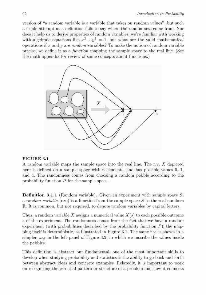
92 Introduction to Probability
version of “a random variable is a variable that takes on random values”, but sucha feeble attempt at a definition fails to say where the randomness come from. Nordoes it help us to derive properties of random variables: we’re familiar with workingwith algebraic equations like x2 + y2 = 1, but what are the valid mathematicaloperations if x and y are random variables? To make the notion of random variableprecise, we define it as a function mapping the sample space to the real line. (Seethe math appendix for review of some concepts about functions.)
X
0 1 4
s1 s3
s4
s2
s5 s6
FIGURE 3.1
A random variable maps the sample space into the real line. The r.v. X depictedhere is defined on a sample space with 6 elements, and has possible values 0, 1,and 4. The randomness comes from choosing a random pebble according to theprobability function P for the sample space.
Definition 3.1.1 (Random variable). Given an experiment with sample space S,a random variable (r.v.) is a function from the sample space S to the real numbersR. It is common, but not required, to denote random variables by capital letters.
Thus, a random variable X assigns a numerical value X(s) to each possible outcomes of the experiment. The randomness comes from the fact that we have a randomexperiment (with probabilities described by the probability function P ); the map-ping itself is deterministic, as illustrated in Figure 3.1. The same r.v. is shown in asimpler way in the left panel of Figure 3.2, in which we inscribe the values insidethe pebbles.
This definition is abstract but fundamental; one of the most important skills todevelop when studying probability and statistics is the ability to go back and forthbetween abstract ideas and concrete examples. Relatedly, it is important to workon recognizing the essential pattern or structure of a problem and how it connects
Random variables and their distributions 93
to problems you have studied previously. We will often discuss stories that involvetossing coins or drawing balls from urns because they are simple, convenient sce-narios to work with, but many other problems are isomorphic: they have the sameessential structure, but in a di↵erent guise.
To start, let’s consider a coin-tossing example. The structure of the problem is thatwe have a sequence of trials where there are two possible outcomes for each trial.Here we think of the possible outcomes as H (Heads) and T (Tails), but we couldjust as well think of them as “success” and “failure” or as 1 and 0, for example.
Example 3.1.2 (Coin tosses). Consider an experiment where we toss afair coin twice. The sample space consists of four possible outcomes: S ={HH,HT, TH, TT}. Here are some random variables on this space (for practice,you can think up some of your own). Each r.v. is a numerical summary of someaspect of the experiment.
• Let X be the number of Heads. This is a random variable with possible values 0,1, and 2. Viewed as a function, X assigns the value 2 to the outcome HH, 1 tothe outcomes HT and TH, and 0 to the outcome TT . That is,
X(HH) = 2, X(HT ) = X(TH) = 1, X(TT ) = 0.
• Let Y be the number of Tails. In terms of X, we have Y = 2�X. In other words,Y and 2�X are the same r.v.: Y (s) = 2�X(s) for all s.
• Let I be 1 if the first toss lands Heads and 0 otherwise. Then I assigns the value 1to the outcomes HH and HT and 0 to the outcomes TH and TT . This r.v. is anexample of what is called an indicator random variable since it indicates whetherthe first toss lands Heads, using 1 to mean “yes” and 0 to mean “no”.
We can also encode the sample space as {(1, 1), (1, 0), (0, 1), (0, 0)}, where 1 is thecode for Heads and 0 is the code for Tails. Then we can give explicit formulas forX,Y, I:
X(s1
, s2
) = s1
+ s2
, Y (s1
, s2
) = 2� s1
� s2
, I(s1
, s2
) = s1
,
where for simplicity we write X(s1
, s2
) to mean X((s1
, s2
)), etc.
For most r.v.s we will consider, it is tedious or infeasible to write down an explicitformula in this way. Fortunately, it is usually unnecessary to do so, since (as wesaw in this example) there are other ways to define an r.v., and (as we will seethroughout the rest of this book) there are many ways to study the properties ofan r.v. other than by doing computations with an explicit formula for what it mapseach outcome s to. ⇤As in the previous chapters, for a sample space with a finite number of outcomeswe can visualize the outcomes as pebbles, with the mass of a pebble correspondingto its probability, such that the total mass of the pebbles is 1. A random variablesimply labels each pebble with a number. Figure 3.2 shows two random variables

94 Introduction to Probability
defined on the same sample space: the pebbles or outcomes are the same, but thereal numbers assigned to the outcomes are di↵erent.
1
4
1
0 1
0 5.3
3
2
9 0
-2s1 s3
s4
s2
s5 s6
s1 s3
s4
s2
s5 s6
FIGURE 3.2
Two random variables defined on the same sample space.
As we’ve mentioned earlier, the source of the randomness in a random variable isthe experiment itself, in which a sample outcome s 2 S is chosen according to aprobability function P . Before we perform the experiment, the outcome s has notyet been realized, so we don’t know the value of X, though we could calculate theprobability thatX will take on a given value or range of values. After we perform theexperiment and the outcome s has been realized, the random variable crystallizesinto the numerical value X(s).
Random variables provide numerical summaries of the experiment in question. Thisis very handy because the sample space of an experiment is often incredibly com-plicated or high-dimensional, and the outcomes s 2 S may be non-numeric. Forexample, the experiment may be to collect a random sample of people in a certaincity and ask them various questions, which may have numeric (e.g., age or height)or non-numeric (e.g., political party or favorite movie) answers. The fact that r.v.stake on numerical values is a very convenient simplification compared to having towork with the full complexity of S at all times.
3.2 Distributions and probability mass functions
There are two main types of random variables used in practice: discrete r.v.s andcontinuous r.v.s. In this chapter and the next, our focus is on discrete r.v.s. Con-tinuous r.v.s are introduced in Chapter 5.
Definition 3.2.1 (Discrete random variable). A random variable X is said to bediscrete if there is a finite list of values a
1
, a2
, . . . , an or an infinite list of valuesa1
, a2
, . . . such that P (X = aj for some j) = 1. If X is a discrete r.v., then the

Random variables and their distributions 95
finite or countably infinite set of values x such that P (X = x) > 0 is called thesupport of X.
Most commonly in applications, the support of a discrete r.v. is a set of integers.In contrast, a continuous r.v. can take on any real value in an interval (possiblyeven the entire real line); such r.v.s are defined more precisely in Chapter 5. Itis also possible to have an r.v. that is a hybrid of discrete and continuous, suchas by flipping a coin and then generating a discrete r.v. if the coin lands Headsand generating a continuous r.v. if the coin lands Tails. But the starting point forunderstanding such r.v.s is to understand discrete and continuous r.v.s.
Given a random variable, we would like to be able to describe its behavior using thelanguage of probability. For example, we might want to answer questions about theprobability that the r.v. will fall into a given range: if L is the lifetime earnings ofa randomly chosen U.S. college graduate, what is the probability that L exceeds amillion dollars? If M is the number of major earthquakes in California in the nextfive years, what is the probability that M equals 0?
The distribution of a random variable provides the answers to these questions; itspecifies the probabilities of all events associated with the r.v., such as the proba-bility of it equaling 3 and the probability of it being at least 110. We will see thatthere are several equivalent ways to express the distribution of an r.v. For a discreter.v., the most natural way to do so is with a probability mass function, which wenow define.
Definition 3.2.2 (Probability mass function). The probability mass function(PMF) of a discrete r.v. X is the function pX given by pX(x) = P (X = x). Notethat this is positive if x is in the support of X, and 0 otherwise.
h 3.2.3. In writing P (X = x), we are using X = x to denote an event, consistingof all outcomes s to which X assigns the number x. This event is also written as{X = x}; formally, {X = x} is defined as {s 2 S : X(s) = x}, but writing {X = x}is shorter and more intuitive. Going back to Example 3.1.2, if X is the numberof Heads in two fair coin tosses, then {X = 1} consists of the sample outcomesHT and TH, which are the two outcomes to which X assigns the number 1. Since{HT, TH} is a subset of the sample space, it is an event. So it makes sense to talkabout P (X = 1), or more generally, P (X = x). If {X = x} were anything otherthan an event, it would make no sense to calculate its probability! It does not makesense to write “P (X)”; we can only take the probability of an event, not of an r.v.
Let’s look at a few examples of PMFs.
Example 3.2.4 (Coin tosses continued). In this example we’ll find the PMFs ofall the random variables in Example 3.1.2, the example with two fair coin tosses.Here are the r.v.s we defined, along with their PMFs:
• X, the number of Heads. Since X equals 0 if TT occurs, 1 if HT or TH occurs,

96 Introduction to Probability
and 2 if HH occurs, the PMF of X is the function pX given by
pX(0) = P (X = 0) = 1/4,
pX(1) = P (X = 1) = 1/2,
pX(2) = P (X = 2) = 1/4,
and pX(x) = 0 for all other values of x.
• Y = 2�X, the number of Tails. Reasoning as above or using the fact that
P (Y = y) = P (2�X = y) = P (X = 2� y) = pX(2� y),
the PMF of Y is
pY (0) = P (Y = 0) = 1/4,
pY (1) = P (Y = 1) = 1/2,
pY (2) = P (Y = 2) = 1/4,
and pY (y) = 0 for all other values of y.
Note that X and Y have the same PMF (that is, pX and pY are the same function)even though X and Y are not the same r.v. (that is, X and Y are two di↵erentfunctions from {HH,HT, TH, TT} to the real line).
• I, the indicator of the first toss landing Heads. Since I equals 0 if TH or TToccurs and 1 if HH or HT occurs, the PMF of I is
pI(0) = P (I = 0) = 1/2,
pI(1) = P (I = 1) = 1/2,
and pI(i) = 0 for all other values of i.
x
PMF
●
●
●
−1 0 1 2 3
0.0
0.5
1.0
y
PMF
●
●
●
−1 0 1 2 3
0.0
0.5
1.0
−1 0 1 2 3i
PMF
● ●
−1 0 1 2 3
0.0
0.5
1.0
FIGURE 3.3
Left to right: PMFs of X, Y , and I, with X the number of Heads in two fair cointosses, Y the number of Tails, and I the indicator of Heads on the first toss.
The PMFs of X, Y , and I are plotted in Figure 3.3. Vertical bars are drawn tomake it easier to compare the heights of di↵erent points. ⇤

Random variables and their distributions 97
Example 3.2.5 (Sum of die rolls). We roll two fair 6-sided dice. Let T = X + Ybe the total of the two rolls, where X and Y are the individual rolls. The samplespace of this experiment has 36 equally likely outcomes:
S = {(1, 1), (1, 2), . . . , (6, 5), (6, 6)}.
For example, 7 of the 36 outcomes s are shown in the table below, along with thecorresponding values of X,Y, and T . After the experiment is performed, we observevalues for X and Y , and then the observed value of T is the sum of those values.
s X Y X + Y
(1, 2) 1 2 3(1, 6) 1 6 7(2, 5) 2 5 7(3, 1) 3 1 4(4, 3) 4 3 7(5, 4) 5 4 9(6, 6) 6 6 12
Since the dice are fair, the PMF of X is
P (X = j) = 1/6,
for j = 1, 2, . . . , 6 (and P (X = j) = 0 otherwise); we say that X has a Discrete Uni-form distribution on 1, 2, . . . , 6. Similarly, Y is also Discrete Uniform on 1, 2, . . . , 6.
Note that Y has the same distribution as X but is not the same random variableas X. In fact, we have
P (X = Y ) = 6/36 = 1/6.
Two more r.v.s in this experiment with the same distribution as X are 7�X and7�Y . To see this, we can use the fact that for a standard die, 7�X is the value onthe bottom if X is the value on the top. If the top value is equally likely to be anyof the numbers 1, 2, . . . , 6, then so is the bottom value. Note that even though 7�Xhas the same distribution as X, it is never equal to X in a run of the experiment!
Let’s now find the PMF of T . By the naive definition of probability,
P (T = 2) = P (T = 12) = 1/36,
P (T = 3) = P (T = 11) = 2/36,
P (T = 4) = P (T = 10) = 3/36,
P (T = 5) = P (T = 9) = 4/36,
P (T = 6) = P (T = 8) = 5/36,
P (T = 7) = 6/36.
For all other values of t, P (T = t) = 0. We can see directly that the support of T

98 Introduction to Probability
is {2, 3, . . . , 12} just by looking at the possible totals for two dice, but as a check,note that
P (T = 2) + P (T = 3) + · · ·+ P (T = 12) = 1,
which shows that all possibilities have been accounted for. The symmetry propertyof T that appears above, P (T = t) = P (T = 14�t), makes sense since each outcome{X = x, Y = y} which makes T = t has a corresponding outcome {X = 7� x, Y =7� y} of the same probability which makes T = 14� t.
0.00
0.05
0.10
0.15
0.20
t
PMF
●
●
●
●
●
●
●
●
●
●
●
2 3 4 5 6 7 8 9 10 11 12
FIGURE 3.4
PMF of the sum of two die rolls.
The PMF of T is plotted in Figure 3.4; it has a triangular shape, and the symmetrynoted above is very visible. ⇤Example 3.2.6 (Children in a U.S. household). Suppose we choose a householdin the United States at random. Let X be the number of children in the chosenhousehold. Since X can only take on integer values, it is a discrete r.v. The proba-bility that X takes on the value x is proportional to the number of households inthe United States with x children.
Using data from the 2010 General Social Survey [26], we can approximate the pro-portion of households with 0 children, 1 child, 2 children, etc., and hence approxi-mate the PMF of X, which is plotted in Figure 3.5. ⇤We will now state the properties of a valid PMF.
Theorem 3.2.7 (Valid PMFs). Let X be a discrete r.v. with support x1
, x2
, . . .(assume these values are distinct and, for notational simplicity, that the support iscountably infinite; the analogous results hold if the support is finite). The PMF pXof X must satisfy the following two criteria:
• Nonnegative: pX(x) > 0 if x = xj for some j, and pX(x) = 0 otherwise;
• Sums to 1:P1
j=1
pX(xj) = 1.

Random variables and their distributions 99
x
PMF ●
●
●
●
●
●● ● ●
0.0
0.1
0.2
0.3
0.4
0.5
0 1 2 3 4 5 6 7 8
FIGURE 3.5
PMF of the number of children in a randomly selected U.S. household.
Proof. The first criterion is true since probability is nonnegative. The second is truesince X must take on some value, and the events {X = xj} are disjoint, so
1X
j=1
P (X = xj) = P
0
@1[
j=1
{X = xj}
1
A = P (X = x1
or X = x2
or . . . ) = 1.
⌅
Conversely, if distinct values x1
, x2
, . . . are specified and we have a function satisfy-ing the two criteria above, then this function is the PMF of some r.v.; we will showhow to construct such an r.v. in Chapter 5.
We claimed earlier that the PMF is one way of expressing the distribution of adiscrete r.v. This is because once we know the PMF of X, we can calculate theprobability that X will fall into a given subset of the real numbers by summing overthe appropriate values of x, as the next example shows.
Example 3.2.8. Returning to Example 3.2.5, let T be the sum of two fair die rolls.We have already calculated the PMF of T . Now suppose we’re interested in theprobability that T is in the interval [1, 4]. There are only three values in the interval[1, 4] that T can take on, namely, 2, 3, and 4. We know the probability of each ofthese values from the PMF of T , so
P (1 T 4) = P (T = 2) + P (T = 3) + P (T = 4) = 6/36.
⇤In general, given a discrete r.v. X and a set B of real numbers, if we know the PMFof X we can find P (X 2 B), the probability that X is in B, by summing up the

100 Introduction to Probability
heights of the vertical bars at points in B in the plot of the PMF of X. Knowingthe PMF of a discrete r.v. determines its distribution.
3.3 Bernoulli and Binomial
Some distributions are so ubiquitous in probability and statistics that they havetheir own names. We will introduce these named distributions throughout the book,starting with a very simple but useful case: an r.v. that can take on only two possiblevalues, 0 and 1.
Definition 3.3.1 (Bernoulli distribution). An r.v. X is said to have the Bernoullidistribution with parameter p if P (X = 1) = p and P (X = 0) = 1 � p, where0 < p < 1. We write this as X ⇠ Bern(p). The symbol ⇠ is read “is distributed as”.
Any r.v. whose possible values are 0 and 1 has a Bern(p) distribution, with p theprobability of the r.v. equaling 1. This number p in Bern(p) is called the parame-ter of the distribution; it determines which specific Bernoulli distribution we have.Thus there is not just one Bernoulli distribution, but rather a family of Bernoullidistributions, indexed by p. For example, if X ⇠ Bern(1/3), it would be correct butincomplete to say “X is Bernoulli”; to fully specify the distribution of X, we shouldboth say its name (Bernoulli) and its parameter value (1/3), which is the point ofthe notation X ⇠ Bern(1/3).
Any event has a Bernoulli r.v. that is naturally associated with it, equal to 1 if theevent happens and 0 otherwise. This is called the indicator random variable of theevent; we will see that such r.v.s are extremely useful.
Definition 3.3.2 (Indicator random variable). The indicator random variable ofan event A is the r.v. which equals 1 if A occurs and 0 otherwise. We will denotethe indicator r.v. of A by IA or I(A). Note that IA ⇠ Bern(p) with p = P (A).
We often imagine Bernoulli r.v.s using coin tosses, but this is just convenient lan-guage for discussing the following general story.
Story 3.3.3 (Bernoulli trial). An experiment that can result in either a “success”or a “failure” (but not both) is called a Bernoulli trial. A Bernoulli random variablecan be thought of as the indicator of success in a Bernoulli trial: it equals 1 if successoccurs and 0 if failure occurs in the trial. ⇤
Because of this story, the parameter p is often called the success probability ofthe Bern(p) distribution. Once we start thinking about Bernoulli trials, it’s hardnot to start thinking about what happens when we have more than one Bernoullitrial.
Story 3.3.4 (Binomial distribution). Suppose that n independent Bernoulli trials
Random variables and their distributions 101
are performed, each with the same success probability p. Let X be the number ofsuccesses. The distribution of X is called the Binomial distribution with parametersn and p. We write X ⇠ Bin(n, p) to mean that X has the Binomial distributionwith parameters n and p, where n is a positive integer and 0 < p < 1. ⇤Notice that we define the Binomial distribution not by its PMF, but by a storyabout the type of experiment that could give rise to a random variable with aBinomial distribution. The most famous distributions in statistics all have storieswhich explain why they are so often used as models for data, or as the buildingblocks for more complicated distributions.
Thinking about the named distributions first and foremost in terms of their storieshas many benefits. It facilitates pattern recognition, allowing us to see when twoproblems are essentially identical in structure; it often leads to cleaner solutionsthat avoid PMF calculations altogether; and it helps us understand how the nameddistributions are connected to one another. Here it is clear that Bern(p) is the samedistribution as Bin(1, p): the Bernoulli is a special case of the Binomial.
Using the story definition of the Binomial, let’s find its PMF.
Theorem 3.3.5 (Binomial PMF). If X ⇠ Bin(n, p), then the PMF of X is
P (X = k) =
✓n
k
◆pk(1� p)n�k
for k = 0, 1, . . . , n (and P (X = k) = 0 otherwise).
h 3.3.6. To save writing, it is often left implicit that a PMF is zero wherever it isnot specified to be nonzero, but in any case it is important to understand what thesupport of a random variable is, and good practice to check that PMFs are valid. Iftwo discrete r.v.s have the same PMF, then they also must have the same support.So we sometimes refer to the support of a discrete distribution; this is the supportof any r.v. with that distribution.
Proof. An experiment consisting of n independent Bernoulli trials produces a se-quence of successes and failures. The probability of any specific sequence of k suc-cesses and n � k failures is pk(1 � p)n�k. There are
�nk
�such sequences, since we
just need to select where the successes are. Therefore, letting X be the number ofsuccesses,
P (X = k) =
✓n
k
◆pk(1� p)n�k
for k = 0, 1, . . . , n, and P (X = k) = 0 otherwise. This is a valid PMF because it isnonnegative and it sums to 1 by the binomial theorem. ⌅
Figure 3.6 shows plots of the Binomial PMF for various values of n and p. Notethat the PMF of the Bin(10, 1/2) distribution is symmetric about 5, but when thesuccess probability is not 1/2, the PMF is skewed. For a fixed number of trials n, Xtends to be larger when the success probability is high and lower when the success

102 Introduction to Probability
probability is low, as we would expect from the story of the Binomial distribution.Also recall that in any PMF plot, the sum of the heights of the vertical bars mustbe 1.
x
PMF
●●
●
●
●
●
●
●
●
●●
0 2 4 6 8 10
0.0
0.1
0.2
0.3
0.4
Bin(10, 1/2)
x
PMF
●
●
● ●
●
●
●
●● ● ●
0 2 4 6 8 10
0.0
0.1
0.2
0.3
0.4
Bin(100, 0.03)
x
PMF
●
●
●
●
●
● ● ● ● ● ●
0 2 4 6 8 100.0
0.1
0.2
0.3
0.4
Bin(10, 1/8)
x
PMF
● ● ● ●●
●
●
● ●
●
0 2 4 6 8 10
0.0
0.1
0.2
0.3
0.4
Bin(9, 4/5)
FIGURE 3.6
Some Binomial PMFs. In the lower left, we plot the Bin(100, 0.03) PMF between 0and 10 only, as the probability of more than 10 successes is close to 0.
We’ve used Story 3.3.4 to find the Bin(n, p) PMF. The story also gives us a straight-forward proof of the fact that if X is Binomial, then n�X is also Binomial.
Theorem 3.3.7. Let X ⇠ Bin(n, p), and q = 1 � p (we often use q to denote thefailure probability of a Bernoulli trial). Then n�X ⇠ Bin(n, q).
Proof. Using the story of the Binomial, interpret X as the number of successesin n independent Bernoulli trials. Then n � X is the number of failures in thosetrials. Interchanging the roles of success and failure, we have n � X ⇠ Bin(n, q).Alternatively, we can check that n�X has the Bin(n, q) PMF. Let Y = n�X. The

Random variables and their distributions 103
PMF of Y is
P (Y = k) = P (X = n� k) =
✓n
n� k
◆pn�kqk =
✓n
k
◆qkpn�k,
for k = 0, 1, . . . , n. ⌅Corollary 3.3.8. LetX ⇠ Bin(n, p) with p = 1/2 and n even. Then the distributionof X is symmetric about n/2, in the sense that P (X = n/2+ j) = P (X = n/2� j)for all nonnegative integers j.
Proof. By Theorem 3.3.7, n�X is also Bin(n, 1/2), so
P (X = k) = P (n�X = k) = P (X = n� k)
for all nonnegative integers k. Letting k = n/2 + j, the desired result follows. Thisexplains why the Bin(10, 1/2) PMF is symmetric about 5 in Figure 3.6. ⌅Example 3.3.9 (Coin tosses continued). Going back to Example 3.1.2, we nowknow that X ⇠ Bin(2, 1/2), Y ⇠ Bin(2, 1/2), and I ⇠ Bern(1/2). Consistent withTheorem 3.3.7, X and Y = 2�X have the same distribution, and consistent withCorollary 3.3.8, the distribution of X (and of Y ) is symmetric about 1. ⇤
3.4 Hypergeometric
If we have an urn filled with w white and b black balls, then drawing n balls outof the urn with replacement yields a Bin(n,w/(w + b)) distribution for the numberof white balls obtained in n trials, since the draws are independent Bernoulli trials,each with probability w/(w+b) of success. If we instead sample without replacement,as illustrated in Figure 3.7, then the number of white balls follows a Hypergeometricdistribution.
FIGURE 3.7
Hypergeometric story. An urn contains w = 6 white balls and b = 4 black balls. Wesample n = 5 without replacement. The number X of white balls in the sample isHypergeometric; here we observe X = 3.
104 Introduction to Probability
Story 3.4.1 (Hypergeometric distribution). Consider an urn with w white ballsand b black balls. We draw n balls out of the urn at random without replacement,such that all
�w+bn
�samples are equally likely. Let X be the number of white balls in
the sample. Then X is said to have the Hypergeometric distribution with parametersw, b, and n; we denote this by X ⇠ HGeom(w, b, n). ⇤As with the Binomial distribution, we can obtain the PMF of the Hypergeometricdistribution from the story.
Theorem 3.4.2 (Hypergeometric PMF). If X ⇠ HGeom(w, b, n), then the PMFof X is
P (X = k) =
�wk
��b
n�k
��w+bn
� ,
for integers k satisfying 0 k w and 0 n�k b, and P (X = k) = 0 otherwise.
Proof. To get P (X = k), we first count the number of possible ways to draw exactlyk white balls and n � k black balls from the urn (without distinguishing betweendi↵erent orderings for getting the same set of balls). If k > w or n � k > b, thenthe draw is impossible. Otherwise, there are
�wk
��b
n�k
�ways to draw k white and
n� k black balls by the multiplication rule, and there are�w+bn
�total ways to draw
n balls. Since all samples are equally likely, the naive definition of probability gives
P (X = k) =
�wk
��b
n�k
��w+bn
�
for integers k satisfying 0 k w and 0 n�k b. This PMF is valid because thenumerator, summed over all k, equals
�w+bn
�by Vandermonde’s identity (Example
1.5.3), so the PMF sums to 1. ⌅
The Hypergeometric distribution comes up in many scenarios which, on the surface,have little in common with white and black balls in an urn. The essential structureof the Hypergeometric story is that items in a population are classified using twosets of tags: in the urn story, each ball is either white or black (this is the first set oftags), and each ball is either sampled or not sampled (this is the second set of tags).Furthermore, at least one of these sets of tags is assigned completely at random(in the urn story, the balls are sampled randomly, with all sets of the correct sizeequally likely). Then X ⇠ HGeom(w, b, n) represents the number of twice-taggeditems: in the urn story, balls that are both white and sampled.
The next two examples show seemingly dissimilar scenarios that are nonethelessisomorphic to the urn story.
Example 3.4.3 (Elk capture-recapture). A forest hasN elk. Today,m of the elk arecaptured, tagged, and released into the wild. At a later date, n elk are recapturedat random. Assume that the recaptured elk are equally likely to be any set of nof the elk, e.g., an elk that has been captured does not learn how to avoid beingcaptured again.

Random variables and their distributions 105
By the story of the Hypergeometric, the number of tagged elk in the recapturedsample has the HGeom(m,N �m,n) distribution. The m tagged elk in this storycorrespond to the white balls and the N �m untagged elk correspond to the blackballs. Instead of sampling n balls from the urn, we recapture n elk from the forest.
⇤
Example 3.4.4 (Aces in a poker hand). In a five-card hand drawn at random from awell-shu✏ed standard deck, the number of aces in the hand has the HGeom(4, 48, 5)distribution, which can be seen by thinking of the aces as white balls and the non-aces as black balls.
Using the Hypergeometric PMF, the probability that the hand has exactly threeaces is
�4
3
��48
2
��52
5
� = 0.0017%.
⇤
The following table summarizes how the above examples can be thought of in termsof two sets of tags. In each example, the r.v. of interest is the number of itemsfalling into both the second and the fourth columns: white and sampled, taggedand recaptured, ace and in one’s hand.
Story First set of tags Second set of tags
urn white black sampled not sampledelk tagged untagged recaptured not recaptured
cards ace not ace in hand not in hand
The next theorem describes a symmetry between two Hypergeometric distributionswith di↵erent parameters; the proof follows from swapping the two sets of tags inthe Hypergeometric story.
Theorem 3.4.5. The HGeom(w, b, n) and HGeom(n,w + b � n,w) distributionsare identical. That is, if X ⇠ HGeom(w, b, n) and Y ⇠ HGeom(n,w + b � n,w),then X and Y have the same distribution.
Proof. Using the story of the Hypergeometric, imagine an urn with w whiteballs, b black balls, and a sample of size n made without replacement. Let X ⇠HGeom(w, b, n) be the number of white balls in the sample, thinking of white/blackas the first set of tags and sampled/not sampled as the second set of tags. LetY ⇠ HGeom(n,w + b � n,w) be the number of sampled balls among the whiteballs, thinking of sampled/not sampled as the first set of tags and white/black asthe second set of tags. Both X and Y count the number of white sampled balls, sothey have the same distribution.
106 Introduction to Probability
Alternatively, we can check algebraically that X and Y have the same PMF:
P (X = k) =
�wk
��b
n�k
��w+bn
� =w!
k!(w�k)!b!
(n�k)!(b�n+k)!
(w+b)!n!(w+b�n)!
=w!b!n!(w + b� n)!
k!(w � k)!(n� k)!(b� n+ k)!,
P (Y = k) =
�nk
��w+b�nw�k
��w+bw
� =n!
k!(n�k)!(w+b�n)!
(w�k)!(b�n+k)!
(w+b)!w!b!
=w!b!n!(w + b� n)!
k!(w � k)!(n� k)!(b� n+ k)!.
We prefer the story proof because it is less tedious and more memorable. ⌅h 3.4.6 (Binomial vs. Hypergeometric). The Binomial and Hypergeometric distri-butions are often confused. Both are discrete distributions taking on integer valuesbetween 0 and n for some n, and both can be interpreted as the number of successesin n Bernoulli trials (for the Hypergeometric, each tagged elk in the recaptured sam-ple can be considered a success and each untagged elk a failure). However, a crucialpart of the Binomial story is that the Bernoulli trials involved are independent. TheBernoulli trials in the Hypergeometric story are dependent, since the sampling isdone without replacement: knowing that one elk in our sample is tagged decreasesthe probability that the second elk will also be tagged.
3.5 Discrete Uniform
A very simple story, closely connected to the naive definition of probability, describespicking a random number from some finite set of possibilities.
Story 3.5.1 (Discrete Uniform distribution). Let C be a finite, nonempty set ofnumbers. Choose one of these numbers uniformly at random (i.e., all values in Care equally likely). Call the chosen number X. Then X is said to have the DiscreteUniform distribution with parameter C; we denote this by X ⇠ DUnif(C). ⇤The PMF of X ⇠ DUnif(C) is
P (X = x) =1
|C|
for x 2 C (and 0 otherwise), since a PMF must sum to 1. As with questionsbased on the naive definition of probability, questions based on a Discrete Uniformdistribution reduce to counting problems. Specifically, for X ⇠ DUnif(C) and anyA ✓ C, we have
P (X 2 A) =|A||C| .
Example 3.5.2 (Random slips of paper). There are 100 slips of paper in a hat,each of which has one of the numbers 1, 2, . . . , 100 written on it, with no numberappearing more than once. Five of the slips are drawn, one at a time.

Random variables and their distributions 107
First consider random sampling with replacement (with equal probabilities).
(a) What is the distribution of how many of the drawn slips have a value of at least80 written on them?
(b) What is the distribution of the value of the jth draw (for 1 j 5)?
(c) What is the probability that the number 100 is drawn at least once?
Now consider random sampling without replacement (with all sets of five slipsequally likely to be chosen).
(d) What is the distribution of how many of the drawn slips have a value of at least80 written on them?
(e) What is the distribution of the value of the jth draw (for 1 j 5)?
(f) What is the probability that the number 100 is drawn at least once?
Solution:
(a) By the story of the Binomial, the distribution is Bin(5, 0.21).
(b) Let Xj be the value of the jth draw. By symmetry, Xj ⇠ DUnif(1, 2, . . . , 100).
(c) Taking complements,
P (Xj = 100 for at least one j) = 1� P (X1
6= 100, . . . , X5
6= 100).
By the naive definition of probability, this is
1� (99/100)5 ⇡ 0.049.
This solution just uses new notation for concepts from Chapter 1. It is useful tohave this new notation since it is compact and flexible. In the above calculation, itis important to see why
P (X1
6= 100, . . . , X5
6= 100) = P (X1
6= 100) . . . P (X5
6= 100).
This follows from the naive definition in this case, but a more general way to thinkabout such statements is through independence of r.v.s, a concept discussed in detailin Section 3.8.
(d) By the story of the Hypergeometric, the distribution is HGeom(21, 79, 5).
(e) Let Yj be the value of the jth draw. By symmetry, Yj ⇠ DUnif(1, 2, . . . , 100).Here learning any Yi gives information about the other values (so Y
1
, . . . , Y5
are notindependent, as defined in Section 3.8), but symmetry still holds since, uncondi-tionally, the jth slip drawn is equally likely to be any of the slips.

108 Introduction to Probability
(f) The events Y1
= 100, . . . , Y5
= 100 are disjoint since we are now samplingwithout replacement, so
P (Yj = 100 for some j) = P (Y1
= 100) + · · ·+ P (Y5
= 100) = 0.05.
Sanity check : This answer makes sense intuitively since we can just as well think offirst choosing five random slips out of 100 blank slips and then randomly writingthe numbers from 1 to 100 on the slips, which gives a 5/100 chance that the number100 is on one of the five chosen slips.
It would be bizarre if the answer to (c) were greater than or equal to the answerto (f), since sampling without replacement makes it easier to find the number 100.(For the same reason, when searching for a lost possession it makes more sense tosample locations without replacement than with replacement.) But it makes sensethat the answer to (c) is only slightly less than the answer to (f), since it is unlikelyin (c) that the same slip will be sampled more than once (though by the birthdayproblem it’s less unlikely than many people would guess). ⇤
3.6 Cumulative distribution functions
Another function that describes the distribution of an r.v. is the cumulative distri-bution function (CDF). Unlike the PMF, which only discrete r.v.s possess, the CDFis defined for all r.v.s.
Definition 3.6.1. The cumulative distribution function (CDF) of an r.v. X is thefunction FX given by FX(x) = P (X x). When there is no risk of ambiguity, wesometimes drop the subscript and just write F (or some other letter) for a CDF.
The next example demonstrates that for discrete r.v.s, we can freely convert betweenCDF and PMF.
Example 3.6.2. Let X ⇠ Bin(4, 1/2). Figure 3.8 shows the PMF and CDF of X.
• From PMF to CDF : To find P (X 1.5), which is the CDF evaluated at 1.5, wesum the PMF over all values of the support that are less than or equal to 1.5:
P (X 1.5) = P (X = 0) + P (X = 1) =
✓1
2
◆4
+ 4
✓1
2
◆4
=5
16.
Similarly, the value of the CDF at an arbitrary point x is the sum of the heightsof the vertical bars of the PMF at values less than or equal to x.
• From CDF to PMF : The CDF of a discrete r.v. consists of jumps and flat regions.The height of a jump in the CDF at x is equal to the value of the PMF at x. Forexample, in Figure 3.8, the height of the jump in the CDF at 2 is the same as the

Random variables and their distributions 109
0 1 2 3 4
0.0
0.2
0.4
0.6
0.8
1.0
x
PMF
●
●
●
●
●
0 1 2 3 4
0.0
0.2
0.4
0.6
0.8
1.0
x
CDF
●
● ●
● ●
● ●
● ●
●
P(X = 2)P(X = 2)
FIGURE 3.8
Bin(4, 1/2) PMF and CDF. The height of the vertical bar P (X = 2) in the PMF isalso the height of the jump in the CDF at 2.
height of the corresponding vertical bar in the PMF; this is indicated in the figurewith curly braces.
The flat regions of the CDF correspond to values outside the support of X, so thePMF is equal to 0 in those regions.
⇤Valid CDFs satisfy the following criteria.
Theorem 3.6.3 (Valid CDFs). Any CDF F has the following properties.
• Increasing: If x1
x2
, then F (x1
) F (x2
).
• Right-continuous: As in Figure 3.8, the CDF is continuous except possibly forhaving some jumps. Wherever there is a jump, the CDF is continuous from theright. That is, for any a, we have
F (a) = limx!a+
F (x).
• Convergence to 0 and 1 in the limits:
limx!�1
F (x) = 0 and limx!1
F (x) = 1.
Proof. The above criteria are true for all CDFs, but for simplicity (and since thischapter focuses on discrete r.v.s) we will only prove it for the case where F is theCDF of a discrete r.v. X whose possible values are 0, 1, 2, . . . . As an example ofhow to visualize the criteria, consider Figure 3.8: the CDF shown there is increasing(with some flat regions), continuous from the right (it is continuous except at jumps,

110 Introduction to Probability
and each jump has an open dot at the bottom and a closed dot at the top), and itconverges to 0 as x ! �1 and to 1 as x ! 1 (in this example, it actually reaches 0and 1; in some examples, one or both of these values may be approached but neverreached).
The first criterion is true since the event {X x1
} is a subset of the event {X x2
},so P (X x
1
) P (X x2
) (this does not depend on X being discrete).
For the second criterion, note that
P (X x) = P (X bxc),
where bxc is the greatest integer less than or equal to x. For example, P (X 4.9) =P (X 4) since X is integer-valued. So F (a+ b) = F (a) for any b > 0 that is smallenough so that a + b < bac + 1, e.g., for a = 4.9, this holds for 0 < b < 0.1. Thisimplies F (a) = limx!a+ F (x) (in fact, it’s much stronger since it says F (x) equalsF (a) when x is close enough to a and on the right).
For the third criterion, we have F (x) = 0 for x < 0, and
limx!1
F (x) = limx!1
P (X bxc) = limx!1
bxcX
n=0
P (X = n) =1X
n=0
P (X = n) = 1.
⌅
The converse is true too: we will show in Chapter 5 that given any function Fmeeting these criteria, we can construct a random variable whose CDF is F .
To recap, we have now seen three equivalent ways of expressing the distribution ofa random variable. Two of these are the PMF and the CDF: we know these twofunctions contain the same information, since we can always figure out the CDFfrom the PMF and vice versa. Generally the PMF is easier to work with for discreter.v.s, since evaluating the CDF requires a summation.
A third way to describe a distribution is with a story that explains (in a preciseway) how the distribution can arise. We used the stories of the Binomial and Hyper-geometric distributions to derive the corresponding PMFs. Thus the story and thePMF also contain the same information, though we can often achieve more intuitiveproofs with the story than with PMF calculations.
3.7 Functions of random variables
In this section we will discuss what it means to take a function of a random variable,and we will build understanding for why a function of a random variable is a random

Random variables and their distributions 111
variable. That is, ifX is a random variable, thenX2, eX , and sin(X) are also randomvariables, as is g(X) for any function g : R ! R.
For example, imagine that two basketball teams (A and B) are playing a seven-game match, and let X be the number of wins for team A (so X ⇠ Bin(7, 1/2) ifthe teams are evenly matched and the games are independent). Let g(x) = 7 � x,and let h(x) = 1 if x � 4 and h(x) = 0 if x < 4. Then g(X) = 7�X is the numberof wins for team B, and h(X) is the indicator of team A winning the majority ofthe games. Since X is an r.v., both g(X) and h(X) are also r.v.s.
To see how to define functions of an r.v. formally, let’s rewind a bit. At the beginningof this chapter, we considered a random variable X defined on a sample space with6 elements. Figure 3.1 used arrows to illustrate how X maps each pebble in thesample space to a real number, and the left half of Figure 3.2 showed how we canequivalently imagine X writing a real number inside each pebble.
Now we can, if we want, apply the same function g to all the numbers inside thepebbles. Instead of the numbers X(s
1
) through X(s6
), we now have the numbersg(X(s
1
)) through g(X(s6
)), which gives a new mapping from sample outcomes toreal numbers—we’ve created a new random variable, g(X).
Definition 3.7.1 (Function of an r.v.). For an experiment with sample space S,an r.v. X, and a function g : R ! R, g(X) is the r.v. that maps s to g(X(s)) for alls 2 S.
Taking g(x) =px for concreteness, Figure 3.9 shows that g(X) is the composition of
the functions X and g, saying “first apply X, then apply g”. Figure 3.10 representsg(X) more succinctly by directly labeling the sample outcomes. Both figures showus that g(X) is an r.v.; if X crystallizes to 4, then g(X) crystallizes to 2.
Given a discrete r.v. X with a known PMF, how can we find the PMF of Y = g(X)?In the case where g is a one-to-one function, the answer is straightforward: thesupport of Y is the set of all g(x) with x in the support of X, and
P (Y = g(x)) = P (g(X) = g(x)) = P (X = x).
The case where Y = g(X) with g one-to-one is illustrated in the following tables;the idea is that if the distinct possible values of X are x
1
, x2
, . . . with probabilitiesp1
, p2
, . . . (respectively), then the distinct possible values of Y are g(x1
), g(x2
), . . . ,with the same list p
1
, p2
, . . . of probabilities.
x P (X = x)
x1
p1
x2
p2
x3
p3
......
PMF of X, in table form
y P (Y = y)
g(x1
) p1
g(x2
) p2
g(x3
) p3
......
PMF of Y , in table form
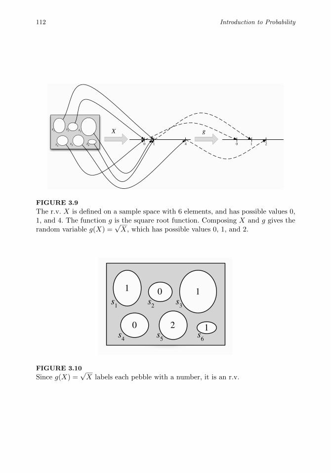
112 Introduction to Probability
X
0 1 4
g
0 1 2
s1 s3
s4
s2
s5 s6
FIGURE 3.9
The r.v. X is defined on a sample space with 6 elements, and has possible values 0,1, and 4. The function g is the square root function. Composing X and g gives therandom variable g(X) =
pX, which has possible values 0, 1, and 2.
1
2
1
0 1
0s1 s3
s4
s2
s5 s6
FIGURE 3.10
Since g(X) =pX labels each pebble with a number, it is an r.v.

Random variables and their distributions 113
This suggests a strategy for finding the PMF of an r.v. with an unfamiliar distri-bution: try to express the r.v. as a one-to-one function of an r.v. with a knowndistribution. The next example illustrates this method.
Example 3.7.2 (Random walk). A particle moves n steps on a number line. Theparticle starts at 0, and at each step it moves 1 unit to the right or to the left,with equal probabilities. Assume all steps are independent. Let Y be the particle’sposition after n steps. Find the PMF of Y .
Solution:
Consider each step to be a Bernoulli trial, where right is considered a success andleft is considered a failure. Then the number of steps the particle takes to theright is a Bin(n, 1/2) random variable, which we can name X. If X = j, then theparticle has taken j steps to the right and n � j steps to the left, giving a finalposition of j � (n � j) = 2j � n. So we can express Y as a one-to-one function ofX, namely, Y = 2X � n. Since X takes values in {0, 1, 2, . . . , n}, Y takes values in{�n, 2� n, 4� n, . . . , n}.
The PMF of Y can then be found from the PMF of X:
P (Y = k) = P (2X � n = k) = P (X = (n+ k)/2) =
✓n
n+k2
◆✓1
2
◆n
,
if k is an integer between �n and n (inclusive) such that n+k is an even number. ⇤If g is not one-to-one, then for a given y, there may be multiple values of x suchthat g(x) = y. To compute P (g(X) = y), we need to sum up the probabilities of Xtaking on any of these candidate values of x.
Theorem 3.7.3 (PMF of g(X)). Let X be a discrete r.v. and g : R ! R. Thenthe support of g(X) is the set of all y such that g(x) = y for at least one x in thesupport of X, and the PMF of g(X) is
P (g(X) = y) =X
x:g(x)=y
P (X = x),
for all y in the support of g(X).
Example 3.7.4. Continuing as in the previous example, let D be the particle’sdistance from the origin after n steps. Assume that n is even. Find the PMF of D.
Solution:
We can write D = |Y |; this is a function of Y , but it isn’t one-to-one. The eventD = 0 is the same as the event Y = 0. For k = 2, 4, . . . , n, the event D = k is thesame as the event {Y = k} [ {Y = �k}. So the PMF of D is
P (D = 0) =
✓nn2
◆✓1
2
◆n
,
P (D = k) = P (Y = k) + P (Y = �k) = 2
✓n
n+k2
◆✓1
2
◆n
,

114 Introduction to Probability
for k = 2, 4, . . . , n. In the final step, we used symmetry to see that P (Y = k) =P (Y = �k). ⇤
The same reasoning we have used to handle functions of one random variable canbe extended to deal with functions of multiple random variables. We have alreadyseen an example of this with the addition function (which maps two numbers x, yto their sum x+ y): in Example 3.2.5, we saw how to view T = X + Y as an r.v. inits own right, where X and Y are obtained by rolling dice.
Definition 3.7.5 (Function of two r.v.s). Given an experiment with sample spaceS, if X and Y are r.v.s that map s 2 S to X(s) and Y (s) respectively, then g(X,Y )is the r.v. that maps s to g(X(s), Y (s)).
One way to understand the mapping from S to R represented by the r.v. g(X,Y )is with a table displaying the values of X, Y , and g(X,Y ) under various possibleoutcomes. Interpreting X+Y as an r.v. is intuitive: if we observe X = x and Y = y,then X+Y crystallizes to x+y. For a less familiar example like max(X,Y ), studentsoften are unsure how to interpret it as an r.v. But the idea is the same: if we observeX = x and Y = y, then max(X,Y ) crystallizes to max(x, y).
Example 3.7.6 (Maximum of two die rolls). We roll two fair 6-sided dice. Let Xbe the number on the first die and Y the number on the second die. The followingtable gives the values of X, Y , and max(X,Y ) under 7 of the 36 outcomes in thesample space, analogously to the table in Example 3.2.5.
s X Y max(X,Y )
(1, 2) 1 2 2(1, 6) 1 6 6(2, 5) 2 5 5(3, 1) 3 1 3(4, 3) 4 3 4(5, 4) 5 4 5(6, 6) 6 6 6
So max(X,Y ) does indeed assigns a numerical value to each sample outcome. ThePMF is
P (max(X,Y ) = 1) = 1/36,
P (max(X,Y ) = 2) = 3/36,
P (max(X,Y ) = 3) = 5/36,
P (max(X,Y ) = 4) = 7/36,
P (max(X,Y ) = 5) = 9/36
P (max(X,Y ) = 6) = 11/36.
These values could be obtained just by listing out and counting possibilities, but it

Random variables and their distributions 115
is less tedious and more generalizable to calculate them by, for example, writing
P (max(X,Y ) = 5) = P (X = 5, Y 4) + P (X 4, Y = 5) + P (X = 5, Y = 5)
= 2P (X = 5, Y 4) + 1/36
= 2(4/36) + 1/36 = 9/36.
⇤h 3.7.7 (Category errors and sympathetic magic). Many common mistakes inprobability can be traced to confusing two of the following fundamental objects witheach other: distributions, random variables, events, and numbers. Such mistakes areexamples of category errors. In general, a category error is a mistake that doesn’t justhappen to be wrong, but in fact is necessarily wrong since it is based on the wrongcategory of object. For example, answering the question “How many people live inBoston?” with “�42” or “⇡” or “pink elephants” would be a category error—wemay not know the population size of a city, but we do know that it is a nonnegativeinteger at any point in time. To help avoid being categorically wrong, always thinkabout what category an answer should have.
An especially common category error is to confuse a random variable with its dis-tribution. We call this error sympathetic magic; this term comes from anthropology,where it is used for the belief that one can influence an object by manipulating arepresentation of that object. The following saying sheds light on the distinctionbetween a random variable and its distribution:
The word is not the thing; the map is not the territory. – Alfred Korzybski
We can think of the distribution of a random variable as a map or blueprint de-scribing the r.v. Just as di↵erent houses can share the same blueprint, di↵erent r.v.scan have the same distribution, even if the experiments they summarize, and thesample spaces they map from, are not the same.
Here are two examples of sympathetic magic:
• Given an r.v. X, trying to get the PMF of 2X by multiplying the PMF of X by2. It does not make sense to multiply a PMF by 2, since the probabilities wouldno longer sum to 1. As we saw above, if X takes on values xj with probabilitiespj , then 2X takes on values 2xj with probabilities pj . Therefore the PMF of 2Xis a horizontal stretch of the PMF of X; it is not a vertical stretch, as wouldresult from multiplying the PMF by 2. Figure 3.11 shows the PMF of a discreter.v. X with support {0, 1, 2, 3, 4}, along with the PMF of 2X, which has support{0, 2, 4, 6, 8}. Note that X can take on odd values, but 2X is necessarily even.
• Claiming that because X and Y have the same distribution, X must always equalY , i.e., P (X = Y ) = 1. Just because two r.v.s have the same distribution doesnot mean they are always equal, or ever equal. We saw this in Example 3.2.5.As another example, consider flipping a fair coin once. Let X be the indicator ofHeads and Y = 1�X be the indicator of Tails. Both X and Y have the Bern(1/2)distribution, but the event X = Y is impossible. The PMFs of X and Y are the

116 Introduction to Probability
0.0
0.2
0.4
0.6
0.8
1.0
x
PMF
of X
●
●
●
● ●
0 1 2 3 4 5 6 7 8 9 10
0.0
0.2
0.4
0.6
0.8
1.0
x
PMF
of 2
X
●
●
●
● ●
0 1 2 3 4 5 6 7 8 9 10
FIGURE 3.11
PMF of X (above) and PMF of 2X (below).

Random variables and their distributions 117
same function, but X and Y are di↵erent mappings from the sample space to thereal numbers.
If Z is the indicator of Heads in a second flip (independent of the first flip), thenZ is also Bern(1/2), but Z is not the same r.v. as X. Here
P (Z = X) = P (HH or TT ) = 1/2.
3.8 Independence of r.v.s
Just as we had the notion of independence of events, we can define independence ofrandom variables. Intuitively, if two r.v.s X and Y are independent, then knowingthe value of X gives no information about the value of Y , and vice versa. Thedefinition formalizes this idea.
Definition 3.8.1 (Independence of two r.v.s). Random variables X and Y are saidto be independent if
P (X x, Y y) = P (X x)P (Y y),
for all x, y 2 R. In the discrete case, this is equivalent to the condition
P (X = x, Y = y) = P (X = x)P (Y = y),
for all x, y with x in the support of X and y in the support of Y .
The definition for more than two r.v.s is analogous.
Definition 3.8.2 (Independence of many r.v.s). Random variables X1
, . . . , Xn areindependent if
P (X1
x1
, . . . , Xn xn) = P (X1
x1
) . . . P (Xn xn),
for all x1
, . . . , xn 2 R. For infinitely many r.v.s, we say that they are independent ifevery finite subset of the r.v.s is independent.
Comparing this to the criteria for independence of n events, it may seem strange thatthe independence of X
1
, . . . , Xn requires just one equality, whereas for events weneeded to verify pairwise independence for all
�n2
�pairs, three-way independence for
all�n3
�triplets, and so on. However, upon closer examination of the definition, we see
that independence of r.v.s requires the equality to hold for all possible x1
, . . . , xn—infinitely many conditions! If we can find even a single list of values x
1
, . . . , xn forwhich the above equality fails to hold, then X
1
, . . . , Xn are not independent.
h 3.8.3. If X1
, . . . , Xn are independent, then they are pairwise independent, i.e.,Xi is independent of Xj for i 6= j. The idea behind proving that Xi and Xj are

118 Introduction to Probability
independent is to let all the xk other than xi, xj go to 1 in the definition of inde-pendence, since we already know Xk < 1 is true (though it takes some work to givea complete justification for the limit). But pairwise independence does not implyindependence in general, as we saw in Chapter 2 for events. A simple counterexam-ple is to use the indicator r.v.s corresponding to the pairwise independent but notindependent events A,B,C in Example 2.5.5.
Example 3.8.4. In a roll of two fair dice, if X is the number on the first die andY is the number on the second die, then X + Y is not independent of X � Y . Tosee why, note that
0 = P (X + Y = 12, X � Y = 1) 6= P (X + Y = 12)P (X � Y = 1) =1
36· 5
36.
Since we have found a pair of values (s, d) for which
P (X + Y = s,X � Y = d) 6= P (X + Y = s)P (X � Y = d),
X+Y and X�Y are dependent. This also makes sense intuitively: knowing the sumof the dice is 12 tells us their di↵erence must be 0, so the r.v.s provide informationabout each other. ⇤If X and Y are independent then it is also true, for example, that X2 is independentof Y 3, since if X2 provided information about Y 3 then X would give informationabout Y (using X2 and Y 3 as intermediaries). In general, if X and Y are inde-pendent then any function of X is independent of any function of Y ; we will notgive a formal proof of this here, but it should make sense from the intuition aboutinformation.
Definition 3.8.5 (i.i.d.). We will often work with random variables that are inde-pendent and have the same distribution. We call such r.v.s independent and identi-cally distributed, or i.i.d. for short.
h 3.8.6 (i. vs. i.d.). “Independent” and “identically distributed” are two often-confused but completely di↵erent concepts. Random variables are independent ifthey provide no information about each other; they are identically distributed ifthey have the same PMF (or equivalently, the same CDF). Whether two r.v.s areindependent has nothing to do with whether or not they have the same distribution.We can have r.v.s that are:
• Independent and identically distributed: Let X be the result of a die roll, and letY be the result of a second, independent die roll. Then X and Y are i.i.d.
• Independent and not identically distributed: Let X be the result of a die roll, andlet Y be the closing price of the Dow Jones (a stock market index) a month fromnow. Then X and Y provide no information about each other (one would ferventlyhope), and X and Y do not have the same distribution.
• Dependent and identically distributed: Let X be the number of Heads in n inde-pendent fair coin tosses, and let Y be the number of Tails in those same n tosses.
Random variables and their distributions 119
Then X and Y are both distributed Bin(n, 1/2), but they are highly dependent:if we know X, then we know Y perfectly.
• Dependent and not identically distributed: Let X be the indicator of whether themajority party retains control of the House of Representatives in the U.S. after thenext election, and let Y be the average favorability rating of the majority partyin polls taken within a month of the election. Then X and Y are dependent, andX and Y do not have the same distribution.
By taking a sum of i.i.d. Bernoulli r.v.s, we can write down the story of the Binomialdistribution in an algebraic form.
Theorem 3.8.7. If X ⇠ Bin(n, p), viewed as the number of successes in n indepen-dent Bernoulli trials with success probability p, then we can write X = X
1
+· · ·+Xn
where the Xi are i.i.d. Bern(p).
Proof. Let Xi = 1 if the ith trial was a success, and 0 if the ith trial was a failure.It’s as though we have a person assigned to each trial, and we ask each person toraise their hand if their trial was a success. If we count the number of raised hands(which is the same as adding up the Xi), we get the total number of successes inthe n trials, which is X. ⌅
An important fact about the Binomial distribution is that the sum of independentBinomial r.v.s with the same success probability is another Binomial r.v. The previ-ous theorem gives an easy proof, though we include two others for comparison.
Theorem 3.8.8. If X ⇠ Bin(n, p), Y ⇠ Bin(m, p), and X is independent of Y ,then X + Y ⇠ Bin(n+m, p).
Proof. We present three proofs, since each illustrates a useful technique.
1. LOTP: We can directly find the PMF of X + Y by conditioning on X (or Y ,whichever we prefer) and using the law of total probability:
P (X + Y = k) =kX
j=0
P (X + Y = k|X = j)P (X = j)
=kX
j=0
P (Y = k � j)P (X = j)
=kX
j=0
✓m
k � j
◆pk�jqm�k+j
✓n
j
◆pjqn�j
= pkqn+m�kkX
j=0
✓m
k � j
◆✓n
j
◆
=
✓n+m
k
◆pkqn+m�k.
120 Introduction to Probability
In the second line, we used the independence of X and Y to justify dropping theconditioning in
P (X + Y = k|X = j) = P (Y = k � j|X = j) = P (Y = k � j),
and in the last line, we used the fact that
kX
j=0
✓m
k � j
◆✓n
j
◆=
✓n+m
k
◆
by Vandermonde’s identity. The resulting expression is the Bin(n+m, p) PMF, soX + Y ⇠ Bin(n+m, p).
2. Representation: A much simpler proof is to represent both X and Y as the sumof i.i.d. Bern(p) r.v.s: X = X
1
+ · · ·+Xn and Y = Y1
+ · · ·+ Ym, where the Xi andYj are all i.i.d. Bern(p). Then X + Y is the sum of n+m i.i.d. Bern(p) r.v.s, so itsdistribution, by the previous theorem, is Bin(n+m, p).
3. Story: By the Binomial story, X is the number of successes in n independenttrials and Y is the number of successes in m additional independent trials, all withthe same success probability, so X+Y is the total number of successes in the n+mtrials, which is the story of the Bin(n+m, p) distribution. ⌅
Of course, if we have a definition for independence of r.v.s, we should have ananalogous definition for conditional independence of r.v.s.
Definition 3.8.9 (Conditional independence of r.v.s). Random variables X and Yare conditionally independent given an r.v. Z if for all x, y 2 R and all z in thesupport of Z,
P (X x, Y y|Z = z) = P (X x|Z = z)P (Y y|Z = z).
For discrete r.v.s, an equivalent definition is to require
P (X = x, Y = y|Z = z) = P (X = x|Z = z)P (Y = y|Z = z).
As we might expect from the name, this is the definition of independence, exceptthat we condition on Z = z everywhere, and require the equality to hold for all zin the support of Z.
Definition 3.8.10 (Conditional PMF). For any discrete r.v.sX and Z, the functionP (X = x|Z = z), when considered as a function of x for fixed z, is called theconditional PMF of X given Z = z.
Independence of r.v.s does not imply conditional independence, nor vice versa. Firstlet us show why independence does not imply conditional independence.

Random variables and their distributions 121
Example 3.8.11 (Matching pennies). Consider the simple game called matchingpennies. Each of two players, A and B, has a fair penny. They flip their penniesindependently. If the pennies match, A wins; otherwise, B wins. Let X be 1 if A’spenny lands Heads and �1 otherwise, and define Y similarly for B (the r.v.s X andY are called random signs).
Let Z = XY , which is 1 if A wins and �1 if B wins. Then X and Y are uncondi-tionally independent, but given Z = 1, we know that X = Y (the pennies match).So X and Y are conditionally dependent given Z. ⇤
Example 3.8.12 (Two causes for an alarm to go o↵). As another example, considera fire alarm where only two things can set it o↵: there being a fire, or someonemicrowaving popcorn a bit too long. Suppose that the fire event is independent ofthe popcorn event. Let X be the indicator of there being a fire, Y be the indicatorof someone microwaving popcorn a bit too long, and Z be the indicator of the firealarm going o↵. Mathematically, we can express Z = max(X,Y ).
By assumption, X and Y are independent. But they are conditionally dependentgiven Z since if we hear the fire alarm going o↵ and know that no one was mi-crowaving popcorn, then we know that there must be a fire. Note that this exampleis isomorphic to the “I have only two friends who ever call me” scenario from Ex-ample 2.5.10. ⇤
Next let’s see why conditional independence does not imply independence.
Example 3.8.13 (Mystery opponent). Suppose that you are going to play twogames of tennis against one of two identical twins. Against one of the twins, you areevenly matched, and against the other you have a 3/4 chance of winning. Supposethat you can’t tell which twin you are playing against until after the two games. LetZ be the indicator of playing against the twin with whom you’re evenly matched, andlet X and Y be the indicators of victory in the first and second games, respectively.
Conditional on Z = 1, X and Y are i.i.d. Bern(1/2), and conditional on Z = 0,X and Y are i.i.d. Bern(3/4). So X and Y are conditionally independent given Z.Unconditionally, X and Y are dependent because observing X = 1 makes it morelikely that we are playing the twin who is worse. That is, P (Y = 1|X = 1) > P (Y =1). Past games give us information which helps us infer who our opponent is, whichin turn helps us predict future games! Note that this example is isomorphic to the“random coin” scenario from Example 2.3.7. ⇤
3.9 Connections between Binomial and Hypergeometric
The Binomial and Hypergeometric distributions are connected in two importantways. As we will see in this section, we can get from the Binomial to the Hyperge-
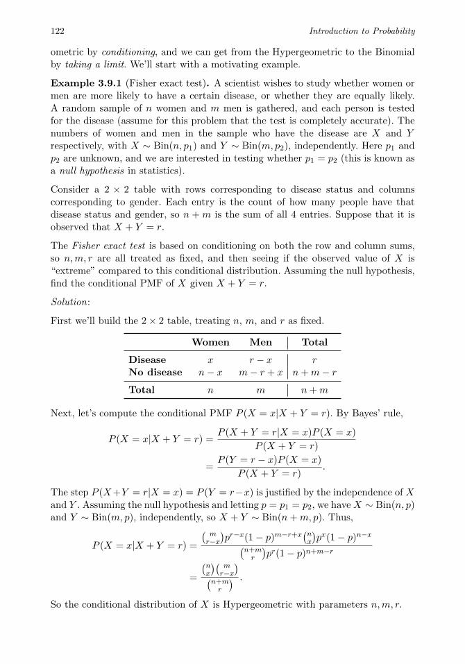
122 Introduction to Probability
ometric by conditioning, and we can get from the Hypergeometric to the Binomialby taking a limit. We’ll start with a motivating example.
Example 3.9.1 (Fisher exact test). A scientist wishes to study whether women ormen are more likely to have a certain disease, or whether they are equally likely.A random sample of n women and m men is gathered, and each person is testedfor the disease (assume for this problem that the test is completely accurate). Thenumbers of women and men in the sample who have the disease are X and Yrespectively, with X ⇠ Bin(n, p
1
) and Y ⇠ Bin(m, p2
), independently. Here p1
andp2
are unknown, and we are interested in testing whether p1
= p2
(this is known asa null hypothesis in statistics).
Consider a 2 ⇥ 2 table with rows corresponding to disease status and columnscorresponding to gender. Each entry is the count of how many people have thatdisease status and gender, so n + m is the sum of all 4 entries. Suppose that it isobserved that X + Y = r.
The Fisher exact test is based on conditioning on both the row and column sums,so n,m, r are all treated as fixed, and then seeing if the observed value of X is“extreme” compared to this conditional distribution. Assuming the null hypothesis,find the conditional PMF of X given X + Y = r.
Solution:
First we’ll build the 2⇥ 2 table, treating n, m, and r as fixed.
Women Men Total
Disease x r � x rNo disease n� x m� r + x n+m� r
Total n m n+m
Next, let’s compute the conditional PMF P (X = x|X + Y = r). By Bayes’ rule,
P (X = x|X + Y = r) =P (X + Y = r|X = x)P (X = x)
P (X + Y = r)
=P (Y = r � x)P (X = x)
P (X + Y = r).
The step P (X+Y = r|X = x) = P (Y = r�x) is justified by the independence of Xand Y . Assuming the null hypothesis and letting p = p
1
= p2
, we haveX ⇠ Bin(n, p)and Y ⇠ Bin(m, p), independently, so X + Y ⇠ Bin(n+m, p). Thus,
P (X = x|X + Y = r) =
�mr�x
�pr�x(1� p)m�r+x
�nx
�px(1� p)n�x
�n+mr
�pr(1� p)n+m�r
=
�nx
��mr�x
��n+mr
� .
So the conditional distribution of X is Hypergeometric with parameters n,m, r.
Random variables and their distributions 123
To understand why the Hypergeometric appeared, seemingly out of nowhere, let’sconnect this problem to the elk story for the Hypergeometric. In the elk story, we areinterested in the distribution of the number of tagged elk in the recaptured sample.By analogy, think of women as tagged elk and men as untagged elk. Instead ofrecapturing r elk at random from the forest, we infect X + Y = r people with thedisease; under the null hypothesis, the set of diseased people is equally likely to beany set of r people. Thus, conditional on X + Y = r, X represents the number ofwomen among the r diseased individuals. This is exactly analogous to the numberof tagged elk in the recaptured sample, which is distributed HGeom(n,m, r).
An interesting fact, which turns out to be useful in statistics, is that the conditionaldistribution of X does not depend on p: unconditionally, X ⇠ Bin(n, p), but pdisappears from the parameters of the conditional distribution! This makes senseupon reflection, since once we know X + Y = r, we can work directly with the factthat we have a population with r diseased and n+m�r undiseased people, withoutworrying about the value of p that originally generated the population. ⇤This motivating example serves as a proof of the following theorem.
Theorem 3.9.2. If X ⇠ Bin(n, p), Y ⇠ Bin(m, p), and X is independent of Y ,then the conditional distribution of X given X + Y = r is HGeom(n,m, r).
In the other direction, the Binomial is a limiting case of the Hypergeometric.
Theorem 3.9.3. If X ⇠ HGeom(w, b, n) and N = w + b ! 1 such that p =w/(w + b) remains fixed, then the PMF of X converges to the Bin(n, p) PMF.
Proof. We take the stated limit of the HGeom(w, b, n) PMF:
P (X = k) =
�wk
��b
n�k
��w+bn
�
=
✓n
k
◆�w+b�nw�k
��w+bw
� by Theorem 3.4.5
=
✓n
k
◆w!
(w � k)!
b!
(b� n+ k)!
(w + b� n)!
(w + b)!
=
✓n
k
◆w(w � 1) . . . (w � k + 1)b(b� 1) . . . (b� n+ k + 1)
(w + b)(w + b� 1) . . . (w + b� n+ 1)
=
✓n
k
◆p�p� 1
N
�. . .�p� k�1
N
�q�q � 1
N
�. . .�q � n�k�1
N
��1� 1
N
� �1� 2
N
�. . .�1� n�1
N
� .
As N ! 1, the denominator goes to 1, and the numerator goes to pkqn�k. Thus
P (X = k) !✓n
k
◆pkqn�k,
which is the Bin(n, p) PMF. ⌅

124 Introduction to Probability
The stories of the Binomial and Hypergeometric provide intuition for this result:given an urn with w white balls and b black balls, the Binomial distribution arisesfrom sampling n balls from the urn with replacement, while the Hypergeometricarises from sampling without replacement. As the number of balls in the urn growsvery large relative to the number of balls that are drawn, sampling with replacementand sampling without replacement become essentially equivalent. In practical terms,this theorem tells us that if N = w + b is large relative to n, we can approximatethe HGeom(w, b, n) PMF by the Bin(n,w/(w + b)) PMF.
The birthday problem implies that it is surprisingly likely that some ball will besampled more than once if sampling with replacement; for example, if 1,200 out of1,000,000 balls are drawn randomly with replacement, then there is about a 51%chance that some ball will be drawn more than once! But this becomes less and lesslikely as N grows, and even if it is likely that there will be a few coincidences, theapproximation can still be reasonable if it is very likely that the vast majority ofballs in the sample are sampled only once each.
3.10 Recap
A random variable (r.v.) is a function assigning a real number to every possibleoutcome of an experiment. The distribution of an r.v. X is a full specification of theprobabilities for the events associated with X, such as {X = 3} and {1 X 5}.The distribution of a discrete r.v. can be defined using a PMF, a CDF, or a story.The PMF of X is the function P (X = x) for x 2 R. The CDF of X is the functionP (X x) for x 2 R. A story for X describes an experiment that could give rise toa random variable with the same distribution as X.
It is important to distinguish between a random variable and its distribution: thedistribution is a blueprint for building the r.v., but di↵erent r.v.s can have the samedistribution, just as di↵erent houses can be built from the same blueprint.
Four named discrete distributions are the Bernoulli, Binomial, Hypergeometric, andDiscrete Uniform. Each of these is actually a family of distributions, indexed byparameters; to fully specify one of these distributions, we need to give both thename and the parameter values.
• A Bern(p) r.v. is the indicator of success in a Bernoulli trial with probability ofsuccess p.
• A Bin(n, p) r.v. is the number of successes in n independent Bernoulli trials, allwith the same probability p of success.
• A HGeom(w, b, n) r.v. is the number of white balls obtained in a sample of size ndrawn without replacement from an urn of w white and b black balls.

Random variables and their distributions 125
• A DUnif(C) r.v. is obtained by randomly choosing an element of the finite set C,with equal probabilities for each element.
A function of a random variable is still a random variable. If we know the PMF ofX, we can find P (g(X) = k), the PMF of g(X), by translating the event {g(X) = k}into an equivalent event involving X, then using the PMF of X.
Two random variables are independent if knowing the value of one r.v. gives noinformation about the value of the other. This is unrelated to whether the two r.v.sare identically distributed. In Chapter 7, we will learn how to deal with dependentrandom variables by considering them jointly rather than separately.
We have now seen four fundamental types of objects in probability: distributions,random variables, events, and numbers. Figure 3.12 shows connections betweenthese four fundamental objects. A CDF can be used as a blueprint for generatingan r.v., and then there are various events describing the behavior of the r.v., suchas the events X x for all x. Knowing the probabilities of these events determinesthe CDF, taking us full circle. For a discrete r.v. we can also use the PMF as ablueprint, and go from distribution to r.v. to events and back again.
CDF FPMF story
name, parameters
XP(X ≤ x) = F(x)
P(X = x)
distributions random variables numbers
X ≤ xX = x
generate
g(X)
P
events
What can happen?
func
tion o
f r.v.
FIGURE 3.12
Four fundamental objects in probability: distributions (blueprints), random vari-ables, events, and numbers. From a CDF F we can generate an r.v. X. From X, wecan generate many other r.v.s by taking functions of X. There are various eventsdescribing the behavior of X. Most notably, for any constant x the events X xand X = x are of interest. Knowing the probabilities of these events for all x givesus the CDF and (in the discrete case) the PMF, taking us full circle.

126 Introduction to Probability
3.11 R
Distributions in R
All of the named distributions that we’ll encounter in this book have been im-plemented in R. In this section we’ll explain how to work with the Binomialand Hypergeometric distributions in R. We will also explain in general howto generate r.v.s from any discrete distribution with a finite support. Typinghelp(distributions) gives a handy list of built-in distributions; many others areavailable through R packages that can be loaded.
In general, for many named discrete distributions, three functions starting with d,p, and r will give the PMF, CDF, and random generation, respectively. Note thatthe function starting with p is not the PMF, but rather is the CDF.
Binomial distribution
The Binomial distribution is associated with the following three R functions:dbinom, pbinom, and rbinom. For the Bernoulli distribution we can just use theBinomial functions with n = 1.
• dbinom is the Binomial PMF. It takes three inputs: the first is the value of xat which to evaluate the PMF, and the second and third are the parameters nand p. For example, dbinom(3,5,0.2) returns the probability P (X = 3) whereX ⇠ Bin(5, 0.2). In other words,
dbinom(3,5,0.2) =
✓5
3
◆(0.2)3(0.8)2 = 0.0512.
• pbinom is the Binomial CDF. It takes three inputs: the first is the value of xat which to evaluate the CDF, and the second and third are the parameters.pbinom(3,5,0.2) is the probability P (X 3) where X ⇠ Bin(5, 0.2). So
pbinom(3,5,0.2) =3X
k=0
✓5
k
◆(0.2)k(0.8)5�k = 0.9933.
• rbinom is a function for generating Binomial random variables. For rbinom, thefirst input is how many r.v.s we want to generate, and the second and thirdinputs are still the parameters. Thus the command rbinom(7,5,0.2) producesrealizations of seven i.i.d. Bin(5, 0.2) r.v.s. When we ran this command, we got
2 1 0 0 1 0 0
but you’ll probably get something di↵erent when you try it!

Random variables and their distributions 127
We can also evaluate PMFs and CDFs at an entire vector of values. For exam-ple, recall that 0:n is a quick way to list the integers from 0 to n. The commanddbinom(0:5,5,0.2) returns 6 numbers, P (X = 0), P (X = 1), . . . , P (X = 5), whereX ⇠ Bin(5, 0.2).
Hypergeometric distribution
The Hypergeometric distribution also has three functions: dhyper, phyper, andrhyper. As one might expect, dhyper is the Hypergeometric PMF, phyper is theHypergeometric CDF, and rhyper generates Hypergeometric r.v.s. Since the Hy-pergeometric distribution has three parameters, each of these functions takes fourinputs. For dhyper and phyper, the first input is the value at which we wish toevaluate the PMF or CDF, and the remaining inputs are the parameters of thedistribution.
Thus dhyper(k,w,b,n) returns the probability P (X = k) where X ⇠HGeom(w, b, n), and phyper(k,w,b,n) returns P (X k). For rhyper, the firstinput is the number of r.v.s we want to generate, and the remaining inputs are theparameters; rhyper(100,w,b,n) generates 100 i.i.d. HGeom(w, b, n) r.v.s.
Discrete distributions with finite support
We can generate r.v.s from any discrete distribution with finite support using thesample command. When we first introduced the sample command, we said that itcan be used in the form sample(n,k) or sample(n,k,replace=TRUE) to sample ktimes from the integers 1 through n, either without or with replacement. For exam-ple, to generate 5 independent DUnif(1, 2, . . . , 100) r.v.s, we can use the commandsample(100,5,replace=TRUE).
It turns out that sample is far more versatile. If we want to sample from the valuesx1
, . . . , xn with probabilities p1
, . . . , pn, we simply create a vector x containing allthe xi and a vector p containing all the pi, then feed them into sample. For example,suppose we are interested in generating realizations of i.i.d. r.v.s X
1
, . . . , X100
whosePMF is
P (Xj = 0) = 0.25,
P (Xj = 1) = 0.5,
P (Xj = 5) = 0.1,
P (Xj = 10) = 0.15,
and P (Xj = x) = 0 for all other values of x. First, we use the c function to createvectors with the support of the distribution and the PMF probabilities.
x <- c(0,1,5,10)
p <- c(0.25,0.5,0.1,0.15)

128 Introduction to Probability
Next, we use the sample command. Here’s how to get 100 samples from the abovePMF:
sample(x,100,prob=p,replace=TRUE)
The inputs are the vector x to sample from, the number of samples to generate (100in this case), the probabilities p of sampling the values in x (if this is omitted, theprobabilities are assumed equal), and whether to sample with replacement.
3.12 Exercises
PMFs and CDFs
1. People are arriving at a party one at a time. While waiting for more people to arrivethey entertain themselves by comparing their birthdays. Let X be the number of peopleneeded to obtain a birthday match, i.e., before person X arrives there are no two peoplewith the same birthday, but when person X arrives there is a match. Find the PMF ofX.
2. (a) Independent Bernoulli trials are performed, with probability 1/2 of success, untilthere has been at least one success. Find the PMF of the number of trials performed.
(b) Independent Bernoulli trials are performed, with probability 1/2 of success, untilthere has been at least one success and at least one failure. Find the PMF of the numberof trials performed.
3. Let X be an r.v. with CDF F , and Y = µ+ �X, where µ and � are real numbers with� > 0. (Then Y is called a location-scale transformation of X; we will encounter thisconcept many times in Chapter 5 and beyond.) Find the CDF of Y , in terms of F .
4. Let n be a positive integer and
F (x) =bxcn
for 0 x n, F (x) = 0 for x < 0, and F (x) = 1 for x > n, where bxc is the greatestinteger less than or equal to x. Show that F is a CDF, and find the PMF that itcorresponds to.
5. (a) Show that p(n) =�1
2
�n+1
for n = 0, 1, 2, . . . is a valid PMF for a discrete r.v.
(b) Find the CDF of a random variable with the PMF from (a).
6. s� Benford’s law states that in a very large variety of real-life data sets, the first digitapproximately follows a particular distribution with about a 30% chance of a 1, an 18%chance of a 2, and in general
P (D = j) = log10
✓j + 1j
◆, for j 2 {1, 2, 3, . . . , 9},
where D is the first digit of a randomly chosen element. Check that this is a valid PMF(using properties of logs, not with a calculator).
7. Bob is playing a video game that has 7 levels. He starts at level 1, and has probabilityp1
of reaching level 2. In general, given that he reaches level j, he has probability pj ofreaching level j + 1, for 1 j 6. Let X be the highest level that he reaches. Find thePMF of X (in terms of p
1
, . . . , p6
).
8. There are 100 prizes, with one worth $1, one worth $2, . . . , and one worth $100. Thereare 100 boxes, each of which contains one of the prizes. You get 5 prizes by picking

Random variables and their distributions 129
random boxes one at a time, without replacement. Find the PMF of how much yourmost valuable prize is worth (as a simple expression in terms of binomial coe�cients).
9. Let F1
and F2
be CDFs, 0 < p < 1, and F (x) = pF1
(x) + (1� p)F2
(x) for all x.
(a) Show directly that F has the properties of a valid CDF (see Theorem 3.6.3). Thedistribution defined by F is called a mixture of the distributions defined by F
1
and F2
.
(b) Consider creating an r.v. in the following way. Flip a coin with probability p ofHeads. If the coin lands Heads, generate an r.v. according to F
1
; if the coin lands Tails,generate an r.v. according to F
2
. Show that the r.v. obtained in this way has CDF F .
10. (a) Is there a discrete distribution with support 1, 2, 3, . . . , such that the value of thePMF at n is proportional to 1/n?
Hint: See the math appendix for a review of some facts about series.
(b) Is there a discrete distribution with support 1, 2, 3, . . . , such that the value of thePMF at n is proportional to 1/n2?
11. s� Let X be an r.v. whose possible values are 0, 1, 2, . . . , with CDF F . In some countries,rather than using a CDF, the convention is to use the function G defined by G(x) =P (X < x) to specify a distribution. Find a way to convert from F to G, i.e., if F is aknown function, show how to obtain G(x) for all real x.
12. (a) Give an example of r.v.s X and Y such that FX(x) FY (x) for all x, where theinequality is strict for some x. Here FX is the CDF of X and FY is the CDF of Y . Forthe example you gave, sketch the CDFs of both X and Y on the same axes. Then sketchtheir PMFs on a second set of axes.
(b) In Part (a), you found an example of two di↵erent CDFs where the first is less thanor equal to the second everywhere. Is it possible to find two di↵erent PMFs where thefirst is less than or equal to the second everywhere? In other words, find discrete r.v.sX and Y such that P (X = x) P (Y = x) for all x, where the inequality is strict forsome x, or show that it is impossible to find such r.v.s.
13. Let X,Y, Z be discrete r.v.s such that X and Y have the same conditional distributiongiven Z, i.e., for all a and z we have
P (X = a|Z = z) = P (Y = a|Z = z).
Show that X and Y have the same distribution (unconditionally, not just when givenZ).
14. Let X be the number of purchases that Fred will make on the online site for a certaincompany (in some specified time period). Suppose that the PMF of X is P (X = k) =e���k/k! for k = 0, 1, 2, . . . . This distribution is called the Poisson distribution withparameter �, and it will be studied extensively in later chapters.
(a) Find P (X � 1) and P (X � 2) without summing infinite series.
(b) Suppose that the company only knows about people who have made at least onepurchase on their site (a user sets up an account to make a purchase, but someonewho has never made a purchase there doesn’t appear in the customer database). If thecompany computes the number of purchases for everyone in their database, then thesedata are draws from the conditional distribution of the number of purchases, given thatat least one purchase is made. Find the conditional PMF of X given X � 1. (Thisconditional distribution is called a truncated Poisson distribution.)
Named distributions
15. Find the CDF of an r.v. X ⇠ DUnif(1, 2, . . . , n).

130 Introduction to Probability
16. Let X ⇠ DUnif(C), and B be a nonempty subset of C. Find the conditional distributionof X, given that X is in B.
17. An airline overbooks a flight, selling more tickets for the flight than there are seats onthe plane (figuring that it’s likely that some people won’t show up). The plane has 100seats, and 110 people have booked the flight. Each person will show up for the flightwith probability 0.9, independently. Find the probability that there will be enough seatsfor everyone who shows up for the flight.
18. s� (a) In the World Series of baseball, two teams (call them A and B) play a sequenceof games against each other, and the first team to win four games wins the series. Letp be the probability that A wins an individual game, and assume that the games areindependent. What is the probability that team A wins the series?
(b) Give a clear intuitive explanation of whether the answer to (a) depends on whetherthe teams always play 7 games (and whoever wins the majority wins the series), or theteams stop playing more games as soon as one team has won 4 games (as is actuallythe case in practice: once the match is decided, the two teams do not keep playing moregames).
19. In a chess tournament, n games are being played, independently. Each game ends in awin for one player with probability 0.4 and ends in a draw (tie) with probability 0.6.Find the PMFs of the number of games ending in a draw, and of the number of playerswhose games end in draws.
20. Suppose that a lottery ticket has probability p of being a winning ticket, independentlyof other tickets. A gambler buys 3 tickets, hoping this will triple the chance of havingat least one winning ticket.
(a) What is the distribution of how many of the 3 tickets are winning tickets?
(b) Show that the probability that at least 1 of the 3 tickets is winning is 3p� 3p2 + p3,in two di↵erent ways: by using inclusion-exclusion, and by taking the complement ofthe desired event and then using the PMF of a certain named distribution.
(c) Show that the gambler’s chances of having at least one winning ticket do not quitetriple (compared with buying only one ticket), but that they do approximately triple ifp is small.
21. s� Let X ⇠ Bin(n, p) and Y ⇠ Bin(m, p), independent of X. Show that X � Y is notBinomial.
22. There are two coins, one with probability p1
of Heads and the other with probabilityp2
of Heads. One of the coins is randomly chosen (with equal probabilities for the twocoins). It is then flipped n � 2 times. Let X be the number of times it lands Heads.
(a) Find the PMF of X.
(b) What is the distribution of X if p1
= p2
?
(c) Give an intuitive explanation of why X is not Binomial for p1
6= p2
(its distribution iscalled a mixture of two Binomials). You can assume that n is large for your explanation,so that the frequentist interpretation of probability can be applied.
23. There are n people eligible to vote in a certain election. Voting requires registration.Decisions are made independently. Each of the n people will register with probability p
1
.Given that a person registers, he or she will vote with probability p
2
. Given that a personvotes, he or she will vote for Kodos (who is one of the candidates) with probability p
3
.What is the distribution of the number of votes for Kodos (give the PMF, fully simplified,or the name of the distribution, including its parameters)?
24. Let X be the number of Heads in 10 fair coin tosses.
(a) Find the conditional PMF of X, given that the first two tosses both land Heads.
(b) Find the conditional PMF of X, given that at least two tosses land Heads.

Random variables and their distributions 131
25. s� Alice flips a fair coin n times and Bob flips another fair coin n + 1 times, resultingin independent X ⇠ Bin(n, 1
2
) and Y ⇠ Bin(n+ 1, 1
2
).
(a) Show that P (X < Y ) = P (n�X < n+ 1� Y ).
(b) Compute P (X < Y ).
Hint: Use (a) and the fact that X and Y are integer-valued.
26. If X ⇠ HGeom(w, b, n), what is the distribution of n�X? Give a short proof.
27. Recall de Montmort’s matching problem from Chapter 1: in a deck of n cards labeled 1through n, a match occurs when the number on the card matches the card’s position inthe deck. Let X be the number of matching cards. Is X Binomial? Is X Hypergeometric?
28. s� There are n eggs, each of which hatches a chick with probability p (independently).Each of these chicks survives with probability r, independently. What is the distributionof the number of chicks that hatch? What is the distribution of the number of chicks thatsurvive? (Give the PMFs; also give the names of the distributions and their parameters,if applicable.)
29. s� A sequence of n independent experiments is performed. Each experiment is a successwith probability p and a failure with probability q = 1 � p. Show that conditional onthe number of successes, all valid possibilities for the list of outcomes of the experimentare equally likely.
30. A company with n women and m men as employees is deciding which employees topromote.
(a) Suppose for this part that the company decides to promote t employees, where1 t n +m, by choosing t random employees (with equal probabilities for each setof t employees). What is the distribution of the number of women who get promoted?
(b) Now suppose that instead of having a predetermined number of promotions togive, the company decides independently for each employee, promoting the employeewith probability p. Find the distributions of the number of women who are promoted,the number of women who are not promoted, and the number of employees who arepromoted.
(c) In the set-up from (b), find the conditional distribution of the number of womenwho are promoted, given that exactly t employees are promoted.
31. Once upon a time, a famous statistician o↵ered tea to a lady. The lady claimed thatshe could tell whether milk had been added to the cup before or after the tea. Thestatistician decided to run some experiments to test her claim.
(a) The lady is given 6 cups of tea, where it is known in advance that 3 will be milk-first and 3 will be tea-first, in a completely random order. The lady gets to taste eachand then guess which 3 were milk-first. Assume for this part that she has no abilitywhatsoever to distinguish milk-first from tea-first cups of tea. Find the probability thatat least 2 of her 3 guesses are correct.
(b) Now the lady is given one cup of tea, with probability 1/2 of it being milk-first.She needs to say whether she thinks it was milk-first. Let p
1
be the lady’s probabilityof being correct given that it was milk-first, and p
2
be her probability of being correctgiven that it was tea-first. She claims that the cup was milk-first. Find the posteriorodds that the cup is milk-first, given this information.
32. In Evan’s history class, 10 out of 100 key terms will be randomly selected to appearon the final exam; Evan must then choose 7 of those 10 to define. Since he knows theformat of the exam in advance, Evan is trying to decide how many key terms he shouldstudy.
(a) Suppose that Evan decides to study s key terms, where s is an integer between 0

132 Introduction to Probability
and 100. Let X be the number of key terms appearing on the exam that he has studied.What is the distribution of X? Give the name and parameters, in terms of s.
(b) Using R or other software, calculate the probability that Evan knows at least 7 ofthe 10 key terms that appear on the exam, assuming that he studies s = 75 key terms.
33. A book has n typos. Two proofreaders, Prue and Frida, independently read the book.Prue catches each typo with probability p
1
and misses it with probability q1
= 1 � p1
,independently, and likewise for Frida, who has probabilities p
2
of catching and q2
= 1�p2
of missing each typo. Let X1
be the number of typos caught by Prue, X2
be the numbercaught by Frida, and X be the number caught by at least one of the two proofreaders.
(a) Find the distribution of X.
(b) For this part only, assume that p1
= p2
. Find the conditional distribution of X1
given that X1
+X2
= t.
34. There are n students at a certain school, of whom X ⇠ Bin(n, p) are Statistics majors.A simple random sample of size m is drawn (“simple random sample” means samplingwithout replacement, with all subsets of the given size equally likely).
(a) Find the PMF of the number of Statistics majors in the sample, using the law of totalprobability (don’t forget to say what the support is). You can leave your answer as asum (though with some algebra it can be simplified, by writing the binomial coe�cientsin terms of factorials and using the binomial theorem).
(b) Give a story proof derivation of the distribution of the number of Statistics majorsin the sample; simplify fully.
Hint: Does it matter whether the students declare their majors before or after therandom sample is drawn?
35. s� Players A and B take turns in answering trivia questions, starting with player Aanswering the first question. Each time A answers a question, she has probability p
1
ofgetting it right. Each time B plays, he has probability p
2
of getting it right.
(a) If A answers m questions, what is the PMF of the number of questions she getsright?
(b) If A answers m times and B answers n times, what is the PMF of the total numberof questions they get right (you can leave your answer as a sum)? Describe exactlywhen/whether this is a Binomial distribution.
(c) Suppose that the first player to answer correctly wins the game (with no predeter-mined maximum number of questions that can be asked). Find the probability that Awins the game.
36. There are n voters in an upcoming election in a certain country, where n is a large, evennumber. There are two candidates: Candidate A (from the Unite Party) and CandidateB (from the Untie Party). Let X be the number of people who vote for Candidate A.Suppose that each voter chooses randomly whom to vote for, independently and withequal probabilities.
(a) Find an exact expression for the probability of a tie in the election (so the candidatesend up with the same number of votes).
(b) Use Stirling’s approximation, which approximates the factorial function as
n! ⇡p2⇡n
⇣ne
⌘n
,
to find a simple approximation to the probability of a tie. Your answer should be of theform 1/
pcn, with c a constant (which you should specify).

Random variables and their distributions 133
37. s� A message is sent over a noisy channel. The message is a sequence x1
, x2
, . . . , xn ofn bits (xi 2 {0, 1}). Since the channel is noisy, there is a chance that any bit might becorrupted, resulting in an error (a 0 becomes a 1 or vice versa). Assume that the errorevents are independent. Let p be the probability that an individual bit has an error(0 < p < 1/2). Let y
1
, y2
, . . . , yn be the received message (so yi = xi if there is no errorin that bit, but yi = 1� xi if there is an error there).
To help detect errors, the nth bit is reserved for a parity check: xn is defined to be 0 ifx1
+ x2
+ · · ·+ xn�1
is even, and 1 if x1
+ x2
+ · · ·+ xn�1
is odd. When the message isreceived, the recipient checks whether yn has the same parity as y
1
+ y2
+ · · ·+ yn�1
. Ifthe parity is wrong, the recipient knows that at least one error occurred; otherwise, therecipient assumes that there were no errors.
(a) For n = 5, p = 0.1, what is the probability that the received message has errorswhich go undetected?
(b) For general n and p, write down an expression (as a sum) for the probability thatthe received message has errors which go undetected.
(c) Give a simplified expression, not involving a sum of a large number of terms, for theprobability that the received message has errors which go undetected.
Hint for (c): Letting
a =X
k even, k�0
n
k
!pk(1� p)n�k and b =
X
k odd, k�1
n
k
!pk(1� p)n�k,
the binomial theorem makes it possible to find simple expressions for a + b and a � b,which then makes it possible to obtain a and b.
Independence of r.v.s
38. (a) Give an example of dependent r.v.s X and Y such that P (X < Y ) = 1.
(b) Give an example of independent r.v.s X and Y such that P (X < Y ) = 1.
39. Give an example of two discrete random variables X and Y on the same sample spacesuch that X and Y have the same distribution, with support {1, 2, . . . , 10}, but theevent X = Y never occurs. If X and Y are independent, is it still possible to constructsuch an example?
40. Suppose X and Y are discrete r.v.s such that P (X = Y ) = 1. This means that X andY always take on the same value.
(a) Do X and Y have the same PMF?
(b) Is it possible for X and Y to be independent?
41. If X,Y, Z are r.v.s such that X and Y are independent and Y and Z are independent,does it follow that X and Z are independent?
Hint: Think about simple and extreme examples.
42. s� Let X be a random day of the week, coded so that Monday is 1, Tuesday is 2, etc. (soX takes values 1, 2, . . . , 7, with equal probabilities). Let Y be the next day afterX (againrepresented as an integer between 1 and 7). Do X and Y have the same distribution?What is P (X < Y )?
43. (a) Is it possible to have two r.v.sX and Y such thatX and Y have the same distributionbut P (X < Y ) � p, where:
• p = 0.9?
• p = 0.99?

134 Introduction to Probability
• p = 0.9999999999999?
• p = 1?
For each, give an example showing it is possible, or prove it is impossible.
Hint: Do the previous question first.
(b) Consider the same question as in Part (a), but now assume that X and Y areindependent. Do your answers change?
44. For x and y binary digits (0 or 1), let x� y be 0 if x = y and 1 if x 6= y (this operationis called exclusive or (often abbreviated to XOR), or addition mod 2 ).
(a) Let X ⇠ Bern(p) and Y ⇠ Bern(1/2), independently. What is the distribution ofX � Y ?
(b) With notation as in (a), is X � Y independent of X? Is X � Y independent of Y ?Be sure to consider both the case p = 1/2 and the case p 6= 1/2.
(c) Let X1
, . . . , Xn be i.i.d. Bern(1/2) r.v.s. For each nonempty subset J of {1, 2, . . . , n},let
YJ =M
j2J
Xj ,
where the notation means to “add” in the � sense all the elements of J ; the order inwhich this is done doesn’t matter since x � y = y � x and (x � y) � z = x � (y � z).Show that YJ ⇠ Bern(1/2) and that these 2n � 1 r.v.s are pairwise independent, butnot independent. For example, we can use this to simulate 1023 pairwise independentfair coin tosses using only 10 independent fair coin tosses.
Hint: Apply the previous parts with p = 1/2. Show that if J and K are two di↵erentnonempty subsets of {1, 2, . . . , n}, then we can write YJ = A+B, YK = A+C, where Aconsists of the Xi with i 2 J\K, B consists of the Xi with i 2 J\Kc, and C consists ofthe Xi with i 2 Jc \K. Then A,B,C are independent since they are based on disjointsets of Xi. Also, at most one of these sets of Xi can be empty. If J \ K = ;, thenYJ = B, YK = C. Otherwise, compute P (YJ = y, YK = z) by conditioning on whetherA = 1.
Mixed practice
45. s� A new treatment for a disease is being tested, to see whether it is better than thestandard treatment. The existing treatment is e↵ective on 50% of patients. It is believedinitially that there is a 2/3 chance that the new treatment is e↵ective on 60% of patients,and a 1/3 chance that the new treatment is e↵ective on 50% of patients. In a pilot study,the new treatment is given to 20 random patients, and is e↵ective for 15 of them.
(a) Given this information, what is the probability that the new treatment is betterthan the standard treatment?
(b) A second study is done later, giving the new treatment to 20 new random patients.Given the results of the first study, what is the PMF for how many of the new patientsthe new treatment is e↵ective on? (Letting p be the answer to (a), your answer can beleft in terms of p.)
46. Independent Bernoulli trials are performed, with success probability 1/2 for each trial.An important question that often comes up in such settings is how many trials toperform. Many controversies have arisen in statistics over the issue of how to analyzedata coming from an experiment where the number of trials can depend on the datacollected so far.
For example, if we can follow the rule “keep performing trials until there are more than

Random variables and their distributions 135
twice as many failures as successes, and then stop”, then naively looking at the ratioof failures to successes (if and when the process stops) will give more than 2:1 ratherthan the true theoretical 1:1 ratio; this could be a very misleading result! However, itmight never happen that there are more than twice as many failures as successes; inthis problem, you will find the probability of that happening.
(a) Two gamblers, A and B, make a series of bets, where each has probability 1/2 ofwinning a bet, but A gets $2 for each win and loses $1 for each loss (a very favorablegame for A!). Assume that the gamblers are allowed to borrow money, so they can anddo gamble forever. Let pk be the probability that A, starting with $k, will ever reach$0, for each k � 0. Explain how this story relates to the original problem, and how theoriginal problem can be solved if we can find pk.
(b) Find pk.
Hint: As in the gambler’s ruin, set up and solve a di↵erence equation for pk. We havepk ! 0 as k ! 1 (you don’t need to prove this, but it should make sense since thegame is so favorable to A, which will result in A’s fortune going to 1; a formal proof,not required here, could be done using the law of large numbers, an important theoremfrom Chapter 10). The solution can be written neatly in terms of the golden ratio.
(c) Find the probability of ever having more than twice as many failures as successeswith independent Bern(1/2) trials, as originally desired.
47. A copy machine is used to make n pages of copies per day. The machine has two traysin which paper gets loaded, and each page used is taken randomly and independentlyfrom one of the trays. At the beginning of the day, the trays are refilled so that theyeach have m pages.
(a) Let pbinom(x, n, p) be the CDF of the Bin(n, p) distribution, evaluated at x. Interms of pbinom, find a simple expression for the probability that both trays haveenough paper on any particular day, when this probability is strictly between 0 and 1(also specify the values of m for which the probability is 0 and the values for which itis 1).
Hint: Be careful about whether inequalities are strict, since the Binomial is discrete.
(b) Using a computer, find the smallest value ofm for which there is at least a 95% chancethat both trays have enough paper on a particular day, for n = 10, n = 100, n = 1000,and n = 10000.
Hint: If you use R, you may find the following commands useful:g <- function(m,n) [your answer from (a)] defines a function g such that g(m,n)is your answer from (a), g(1:100,100) gives the vector (g(1, 100), . . . , g(100, 100)),which(v>0.95) gives the indices of the components of vector v that exceed 0.95, andmin(w) gives the minimum of a vector w.

4
Expectation
4.1 Definition of expectation
In the previous chapter, we introduced the distribution of a random variable, whichgives us full information about the probability that the r.v. will fall into any partic-ular set. For example, we can say how likely it is that the r.v. will exceed 1000, thatit will equal 5, and that it will be in the interval [0, 7]. It can be unwieldy to manageso many probabilities though, so often we want just one number summarizing the“average” value of the r.v.
There are several senses in which the word “average” is used, but by far the mostcommonly used is the mean of an r.v., also known as its expected value. In addition,much of statistics is about understanding variability in the world, so it is oftenimportant to know how “spread out” the distribution is; we will formalize this withthe concepts of variance and standard deviation. As we’ll see, variance and standarddeviation are defined in terms of expected values, so the uses of expected values gofar beyond just computing averages.
Given a list of numbers x1
, x2
, . . . , xn, the familiar way to average them is to addthem up and divide by n. This is called the arithmetic mean, and is defined by
x =1
n
nX
j=1
xj .
More generally, we can define a weighted mean of x1
, . . . , xn as
weighted-mean(x) =nX
j=1
xjpj ,
where the weights p1
, . . . , pn are pre-specified nonnegative numbers that add up to1 (so the unweighted mean x is obtained when pj = 1/n for all j).
The definition of expectation for a discrete r.v. is inspired by the weighted mean ofa list of numbers, with weights given by probabilities.
Definition 4.1.1 (Expectation of a discrete r.v.). The expected value (also calledthe expectation or mean) of a discrete r.v. X whose distinct possible values are
137

138 Introduction to Probability
x1
, x2
, . . . is defined by
E(X) =1X
j=1
xjP (X = xj).
If the support is finite, then this is replaced by a finite sum. We can also write
E(X) =X
x
x|{z}value
P (X = x)| {z }PMF at x
,
where the sum is over the support of X (in any case, xP (X = x) is 0 for any x notin the support). The expectation is undefined if
P1j=1
|xj |P (X = xj) diverges, sincethen the series for E(X) diverges or its value depends on the order in which the xjare listed.
In words, the expected value of X is a weighted average of the possible values thatX can take on, weighted by their probabilities. Let’s check that the definition makessense in two simple examples:
1. Let X be the result of rolling a fair 6-sided die, so X takes on the values1, 2, 3, 4, 5, 6, with equal probabilities. Intuitively, we should be able toget the average by adding up these values and dividing by 6. Using thedefinition, the expected value is
E(X) =1
6(1 + 2 + · · ·+ 6) = 3.5,
as we expected. Note though that X never equals its mean in this exam-ple. This is similar to the fact that the average number of children perhousehold in some country could be 1.8, but that doesn’t mean that atypical household has 1.8 children!
2. Let X ⇠ Bern(p) and q = 1� p. Then
E(X) = 1p+ 0q = p,
which makes sense intuitively since it is between the two possible valuesof X, compromising between 0 and 1 based on how likely each is. This isillustrated in Figure 4.1 for a case with p < 1/2: two pebbles are beingbalanced on a seesaw. For the seesaw to balance, the fulcrum (shown as atriangle) must be at p, which in physics terms is the center of mass.
The frequentist interpretation would be to consider a large number ofindependent Bernoulli trials, each with probability p of success. Writing 1for “success” and 0 for “failure”, in the long run we would expect to havedata consisting of a list of numbers where the proportion of 1’s is veryclose to p. The average of a list of 0’s and 1’s is the proportion of 1’s.
Note that E(X) depends only on the distribution of X. This follows directly fromthe definition, but is worth recording since it is fundamental.

Expectation 139
q p
0 1
p0.5
FIGURE 4.1
Center of mass of two pebbles, depicting that E(X) = p for X ⇠ Bern(p). Here qand p denote the masses of the two pebbles.
Proposition 4.1.2. If X and Y are discrete r.v.s with the same distribution, thenE(X) = E(Y ) (if either side exists).
Proof. In the definition of E(X), we only need to know the PMF of X. ⌅
The converse of the above proposition is false since the expected value is just aone-number summary, not nearly enough to specify the entire distribution; it’s ameasure of where the “center” is but does not determine, for example, how spreadout the distribution is or how likely the r.v. is to be positive. Figure 4.2 shows anexample of two di↵erent PMFs that both have a balancing point or expected valueof 2.
0 1 2 3 4
0.0
0.2
0.4
0.6
0.8
1.0
●
●
●
●
●
0 1 2 3 4
0.0
0.2
0.4
0.6
0.8
1.0
● ●
FIGURE 4.2
The expected value does not determine the distribution: di↵erent PMFs can havethe same balancing point.
h 4.1.3 (Replacing an r.v. by its expectation). For any discrete r.v.X, the expectedvalue E(X) is a number (if it exists). A common mistake is to replace an r.v. byits expectation without justification, which is wrong both mathematically (X isa function, E(X) is a constant) and statistically (it ignores the variability of X),except in the degenerate case where X is a constant.

140 Introduction to Probability
Notation 4.1.4. We often abbreviate E(X) to EX. Similarly, we often abbreviateE(X2) to EX2. Thus EX2 is the expectation of the random variable X2, not thesquare of the number EX. In general, unless the parentheses explicitly indicateotherwise, the expectation is to be taken at the very end. For example, E(X�3)2 isE�(X � 3)2
�, not (E(X � 3))2. As we will see, the order of operations here is very
important!
4.2 Linearity of expectation
The most important property of expectation is linearity : the expected value of asum of r.v.s is the sum of the individual expected values.
Theorem 4.2.1 (Linearity of expectation). For any r.v.s X,Y and any constant c,
E(X + Y ) = E(X) + E(Y ),
E(cX) = cE(X).
The second equation says that we can take out constant factors from an expectation;this is both intuitively reasonable and easily verified from the definition. The firstequation, E(X + Y ) = E(X) + E(Y ), also seems reasonable when X and Y areindependent. What may be surprising is that it holds even ifX and Y are dependent!To build intuition for this, consider the extreme case whereX always equals Y . ThenX + Y = 2X, and both sides of E(X + Y ) = E(X) +E(Y ) are equal to 2E(X), solinearity still holds even in the most extreme case of dependence.
Linearity is true for all r.v.s, not just discrete r.v.s, but in this chapter we will proveit only for discrete r.v.s. Before proving linearity, it is worthwhile to recall somebasic facts about averages. If we have a list of numbers, say (1, 1, 1, 1, 1, 3, 3, 5), wecan calculate their mean by adding all the values and dividing by the length of thelist, so that each element of the list gets a weight of 1
8
:
1
8(1 + 1 + 1 + 1 + 1 + 3 + 3 + 5) = 2.
But another way to calculate the mean is to group together all the 1’s, all the 3’s,and all the 5’s, and then take a weighted average, giving appropriate weights to 1’s,3’s, and 5’s:
5
8· 1 + 2
8· 3 + 1
8· 5 = 2.
This insight—that averages can be calculated in two ways, ungrouped or grouped—is all that is needed to prove linearity! Recall that X is a function which assignsa real number to every outcome s in the sample space. The r.v. X may assignthe same value to multiple sample outcomes. When this happens, our definition of

Expectation 141
expectation groups all these outcomes together into a super-pebble whose weight,P (X = x), is the total weight of the constituent pebbles. This grouping processis illustrated in Figure 4.3 for a hypothetical r.v. taking values in {0, 1, 2}. So ourdefinition of expectation corresponds to the grouped way of taking averages.
0 1
0
02
2
1
1
10 1
0
02
2
1
1
1
FIGURE 4.3
Left: X assigns a number to each pebble in the sample space. Right: Grouping thepebbles by the value that X assigns to them, the 9 pebbles become 3 super-pebbles.The weight of a super-pebble is the sum of the weights of the constituent pebbles.
The advantage of this definition is that it allows us to work with the distribution ofX directly, without returning to the sample space. The disadvantage comes when wehave to prove theorems like this one, for if we have another r.v. Y on the same samplespace, the super-pebbles created by Y are di↵erent from those created from X, withdi↵erent weights P (Y = y); this makes it di�cult to combine
Px xP (X = x) andP
y yP (Y = y).
Fortunately, we know there’s another equally valid way to calculate an average: wecan take a weighted average of the values of individual pebbles. In other words, ifX(s) is the value that X assigns to pebble s, we can take the weighted average
E(X) =X
s
X(s)P ({s}),
where P ({s}) is the weight of pebble s. This corresponds to the ungrouped way oftaking averages. The advantage of this definition is that it breaks down the samplespace into the smallest possible units, so we are now using the same weights P ({s})for every random variable defined on this sample space. If Y is another randomvariable, then
E(Y ) =X
s
Y (s)P ({s}).
Now we can combineP
sX(s)P ({s}) andP
s Y (s)P ({s}), which gives E(X + Y )as desired:
E(X)+E(Y ) =X
s
X(s)P ({s})+X
s
Y (s)P ({s}) =X
s
(X+Y )(s)P ({s}) = E(X+Y ).
Another intuition for linearity of expectation is via the concept of simulation. If

142 Introduction to Probability
we simulate many, many times from the distribution of X, the histogram of thesimulated values will look very much like the true PMF of X. In particular, thearithmetic mean of the simulated values will be very close to the true value of E(X)(the precise nature of this convergence is described by the law of large numbers, animportant theorem that we will discuss in detail in Chapter 10).
Let X and Y be r.v.s summarizing a certain experiment. Suppose we perform theexperiment n times, where n is a very large number, and we write down the valuesrealized by X and Y each time. For each repetition of the experiment, we obtainan X value, a Y value, and (by adding them) an X + Y value. In Figure 4.4, eachrow represents a repetition of the experiment. The left column contains the drawsof X, the middle column contains the draws of Y , and the right column containsthe draws of X + Y .
X Y X + Y
3 4 72 2 46 8 14
10 23 331 �3 �21 0 15 9 144 1 5...
......
1
n
nX
i=1
xi +1
n
nX
i=1
yi =1
n
nX
i=1
(xi + yi)
E(X) + E(Y ) = E(X + Y )
FIGURE 4.4
Intuitive view of linearity of expectation. Each row represents a repetition of theexperiment; the three columns are the realized values of X, Y , and X + Y , respec-tively. Adding all the numbers in the last column is equivalent to summing the firstcolumn and the second column separately, then adding the two column sums. Sothe mean of the last column is the sum of the first and second column means; thisis linearity of expectation.
There are two ways to calculate the sum of all the numbers in the last column. Thestraightforward way is just to add all the numbers in that column. But an equallyvalid way is to add all the numbers in the first column, add all the numbers in thesecond column, and then add the two column sums.
Dividing by n everywhere, what we’ve argued is that the following procedures areequivalent:

Expectation 143
• Taking the arithmetic mean of all the numbers in the last column. By the law oflarge numbers, this is very close to E(X + Y ).
• Taking the arithmetic mean of the first column and the arithmetic mean of thesecond column, then adding the two column means. By the law of large numbers,this is very close to E(X) + E(Y ).
Linearity of expectation thus emerges as a simple fact about arithmetic (we’re justadding numbers in two di↵erent orders)! Notice that nowhere in our argument didwe rely on whether X and Y were independent. In fact, in Figure 4.4, X and Yappear to be dependent: Y tends to be large when X is large, and Y tends to besmall when X is small (in the language of Chapter 7, we say that X and Y arepositively correlated). But this dependence is irrelevant: shu✏ing the draws of Ycould completely alter the pattern of dependence between X and Y , but wouldhave no e↵ect on the column sums.
Linearity is an extremely handy tool for calculating expected values, often allowingus to bypass the definition of expected value altogether. Let’s use linearity to findthe expectations of the Binomial and Hypergeometric distributions.
Example 4.2.2 (Binomial expectation). For X ⇠ Bin(n, p), let’s find E(X) in twoways. By definition of expectation,
E(X) =nX
k=0
kP (X = k) =nX
k=0
k
✓n
k
◆pkqn�k.
From Example 1.5.2, we know k�nk
�= n
�n�1
k�1
�, so
nX
k=0
k
✓n
k
◆pkqn�k = n
nX
k=0
✓n� 1
k � 1
◆pkqn�k
= np
nX
k=1
✓n� 1
k � 1
◆pk�1qn�k
= np
n�1X
j=0
✓n� 1
j
◆pjqn�1�j
= np.
The sum in the penultimate line equals 1 because it is the sum of the Bin(n� 1, p)PMF (or by the binomial theorem). Therefore, E(X) = np.
This proof required us to remember combinatorial identities and manipulate bino-mial coe�cients. Using linearity of expectation, we obtain a much shorter path tothe same result. Let’s write X as the sum of n independent Bern(p) r.v.s:
X = I1
+ · · ·+ In,
where each Ij has expectation E(Ij) = 1p+ 0q = p. By linearity,
E(X) = E(I1
) + · · ·+ E(In) = np.

144 Introduction to Probability
⇤
Example 4.2.3 (Hypergeometric expectation). Let X ⇠ HGeom(w, b, n), inter-preted as the number of white balls in a sample of size n drawn without replacementfrom an urn with w white and b black balls. As in the Binomial case, we can writeX as a sum of Bernoulli random variables,
X = I1
+ · · ·+ In,
where Ij equals 1 if the jth ball in the sample is white and 0 otherwise. By symmetry,Ij ⇠ Bin(p) with p = w/(w+ b), since unconditionally the jth ball drawn is equallylikely to be any of the balls.
Unlike in the Binomial case, the Ij are not independent, since the sampling iswithout replacement: given that a ball in the sample is white, there is a lowerchance that another ball in the sample is white. However, linearity still holds fordependent random variables! Thus,
E(X) = nw/(w + b).
⇤
As another example of the power of linearity, we can give a quick proof of theintuitive idea that “bigger r.v.s have bigger expectations”.
Proposition 4.2.4 (Monotonicity of expectation). Let X and Y be r.v.s such thatX � Y with probability 1. Then E(X) � E(Y ), with equality holding if and onlyif X = Y with probability 1.
Proof. This result holds for all r.v.s, but we will prove it only for discrete r.v.s sincethis chapter focuses on discrete r.vs. The r.v. Z = X � Y is nonnegative (withprobability 1), so E(Z) � 0 since E(Z) is defined as a sum of nonnegative terms.By linearity,
E(X)� E(Y ) = E(X � Y ) � 0,
as desired. If E(X) = E(Y ), then by linearity we also have E(Z) = 0, which impliesthat P (X = Y ) = P (Z = 0) = 1 since if even one term in the sum defining E(Z) ispositive, then the whole sum is positive. ⌅
4.3 Geometric and Negative Binomial
We now introduce two more famous discrete distributions, the Geometric and Neg-ative Binomial, and calculate their expected values.

Expectation 145
Story 4.3.1 (Geometric distribution). Consider a sequence of independentBernoulli trials, each with the same success probability p 2 (0, 1), with trials per-formed until a success occurs. Let X be the number of failures before the firstsuccessful trial. Then X has the Geometric distribution with parameter p; we de-note this by X ⇠ Geom(p). ⇤For example, if we flip a fair coin until it lands Heads for the first time, then the num-ber of Tails before the first occurrence of Heads is distributed as Geom(1/2).
To get the Geometric PMF from the story, imagine the Bernoulli trials as a stringof 0’s (failures) ending in a single 1 (success). Each 0 has probability q = 1� p andthe final 1 has probability p, so a string of k failures followed by one success hasprobability qkp.
Theorem 4.3.2 (Geometric PMF). If X ⇠ Geom(p), then the PMF of X is
P (X = k) = qkp
for k = 0, 1, 2, . . . , where q = 1� p.
This is a valid PMF because
1X
k=0
qkp = p
1X
k=0
qk = p · 1
1� q= 1.
Just as the binomial theorem shows that the Binomial PMF is valid, a geometricseries shows that the Geometric PMF is valid!
Figure 4.3 displays the Geom(0.5) PMF and CDF from k = 0 to k = 6. All Geo-metric PMFs have a similar shape; the greater the success probability p, the morequickly the PMF decays to 0.
0 1 2 3 4 5 6
0.0
0.2
0.4
0.6
0.8
1.0
x
PMF
●
●
●
●● ● ●
0 1 2 3 4 5 6
0.0
0.2
0.4
0.6
0.8
1.0
x
CDF
●
● ●
● ●
● ●
● ●● ●● ●●
FIGURE 4.5
Geom(0.5) PMF and CDF.

146 Introduction to Probability
h 4.3.3 (Conventions for the Geometric). There are di↵ering conventions for thedefinition of the Geometric distribution; some sources define the Geometric as thetotal number of trials, including the success. In this book, the Geometric distributionexcludes the success, and the First Success distribution includes the success.
Definition 4.3.4 (First Success distribution). In a sequence of independentBernoulli trials with success probability p, let Y be the number of trials until thefirst successful trial, including the success. Then Y has the First Success distributionwith parameter p; we denote this by Y ⇠ FS(p).
It is easy to convert back and forth between the two but important to be carefulabout which convention is being used. By definition, if Y ⇠ FS(p) then Y � 1 ⇠Geom(p), and we can convert between the PMFs of Y and Y � 1 by writing P (Y =k) = P (Y � 1 = k � 1). Conversely, if X ⇠ Geom(p), then X + 1 ⇠ FS(p).
Example 4.3.5 (Geometric expectation). Let X ⇠ Geom(p). By definition,
E(X) =1X
k=0
kqkp,
where q = 1 � p. This sum looks unpleasant; it’s not a geometric series because ofthe extra k multiplying each term. But we notice that each term looks similar tokqk�1, the derivative of qk (with respect to q), so let’s start there:
1X
k=0
qk =1
1� q.
This geometric series converges since 0 < q < 1. Di↵erentiating both sides withrespect to q, we get
1X
k=0
kqk�1 =1
(1� q)2.
Finally, if we multiply both sides by pq, we recover the original sum we wanted tofind:
E(X) =1X
k=0
kqkp = pq
1X
k=0
kqk�1 = pq1
(1� q)2=
q
p.
In Chapter 9, Example 9.1.8, we will give a story proof of the same result, based onfirst-step analysis: condition on the result of the first trial in the story interpretationof X. If the first trial is a success, we know X = 0 and if it’s a failure, we have onewasted trial and then are back where we started. ⇤Example 4.3.6 (First Success expectation). Since we can write Y ⇠ FS(p) asY = X + 1 where X ⇠ Geom(p), we have
E(Y ) = E(X + 1) =q
p+ 1 =
1
p.
⇤
Expectation 147
The Negative Binomial distribution generalizes the Geometric distribution: insteadof waiting for just one success, we can wait for any predetermined number r ofsuccesses.
Story 4.3.7 (Negative Binomial distribution). In a sequence of independentBernoulli trials with success probability p, if X is the number of failures beforethe rth success, then X is said to have the Negative Binomial distribution withparameters r and p, denoted X ⇠ NBin(r, p). ⇤Both the Binomial and the Negative Binomial distributions are based on indepen-dent Bernoulli trials; they di↵er in the stopping rule and in what they are counting:the Binomial counts the number of successes in a fixed number of trials, whilethe Negative Binomial counts the number of failures until a fixed number of suc-cesses.
In light of these similarities, it comes as no surprise that the derivation of theNegative Binomial PMF bears a resemblance to the corresponding derivation forthe Binomial.
Theorem 4.3.8 (Negative Binomial PMF). If X ⇠ NBin(r, p), then the PMF ofX is
P (X = n) =
✓n+ r � 1
r � 1
◆prqn
for n = 0, 1, 2 . . . , where q = 1� p.
Proof. Imagine a string of 0’s and 1’s, with 1’s representing successes. The proba-bility of any specific string of n 0’s and r 1’s is prqn. How many such strings arethere? Because we stop as soon as we hit the rth success, the string must terminatein a 1. Among the other n+r�1 positions, we choose r�1 places for the remaining1’s to go. So the overall probability of exactly n failures before the rth success is
P (X = n) =
✓n+ r � 1
r � 1
◆prqn, n = 0, 1, 2, . . .
⌅
Just as a Binomial r.v. can be represented as a sum of i.i.d. Bernoullis, a NegativeBinomial r.v. can be represented as a sum of i.i.d. Geometrics.
Theorem 4.3.9. Let X ⇠ NBin(r, p), viewed as the number of failures before therth success in a sequence of independent Bernoulli trials with success probability p.Then we can write X = X
1
+ · · ·+Xr where the Xi are i.i.d. Geom(p).
Proof. Let X1
be the number of failures until the first success, X2
be the numberof failures between the first success and the second success, and in general, Xi bethe number of failures between the (i� 1)st success and the ith success.
Then X1
⇠ Geom(p) by the story of the Geometric distribution. After the firstsuccess, the number of additional failures until the next success is still Geometric!

148 Introduction to Probability
So X2
⇠ Geom(p), and similarly for all the Xi. Furthermore, the Xi are independentbecause the trials are all independent of each other. Adding the Xi, we get the totalnumber of failures before the rth success, which is X. ⌅
Using linearity, the expectation of the Negative Binomial now follows without anyadditional calculations.
Example 4.3.10 (Negative Binomial expectation). Let X ⇠ NBin(r, p). By theprevious theorem, we can write X = X
1
+ · · ·+Xr, where the Xi are i.i.d. Geom(p).By linearity,
E(X) = E(X1
) + · · ·+ E(Xr) = r · qp.
⇤
The next example is a famous problem in probability and an instructive appli-cation of the Geometric and First Success distributions. It is usually stated as aproblem about collecting coupons, hence its name, but we’ll use toys instead ofcoupons.
Example 4.3.11 (Coupon collector). Suppose there are n types of toys, which youare collecting one by one, with the goal of getting a complete set. When collectingtoys, the toy types are random (as is sometimes the case, for example, with toysincluded in cereal boxes or included with kids’ meals from a fast food restaurant).Assume that each time you collect a toy, it is equally likely to be any of the n types.What is the expected number of toys needed until you have a complete set?
Solution:
Let N be the number of toys needed; we want to find E(N). Our strategy will beto break up N into a sum of simpler r.v.s so that we can apply linearity. So write
N = N1
+N2
+ · · ·+Nn,
where N1
is the number of toys until the first toy type you haven’t seen before(which is always 1, as the first toy is always a new type), N
2
is the additionalnumber of toys until the second toy type you haven’t seen before, and so forth.Figure 4.6 illustrates these definitions with n = 3 toy types.
By the story of the FS distribution, N2
⇠ FS((n�1)/n): after collecting the first toytype, there’s a 1/n chance of getting the same toy you already had (failure) and an(n � 1)/n chance you’ll get something new (success). Similarly, N
3
, the additionalnumber of toys until the third new toy type, is distributed FS((n�2)/n). In general,
Nj ⇠ FS((n� j + 1)/n).

Expectation 149
N1 N2 N3
FIGURE 4.6
Coupon collector, n = 3. Here N1
is the time (number of toys collected) until thefirst new toy type, N
2
is the additional time until the second new type, and N3
is theadditional time until the third new type. The total number of toys for a completeset is N
1
+N2
+N3
.
By linearity,
E(N) = E(N1
) + E(N2
) + E(N3
) + · · ·+ E(Nn)
= 1 +n
n� 1+
n
n� 2+ · · ·+ n
= n
nX
j=1
1
j.
For large n, this is very close to n(log n+ 0.577).
Before we leave this example, let’s take a moment to connect it to our proof ofTheorem 4.3.9, the representation of the Negative Binomial as a sum of i.i.d. Geo-metrics. In both problems, we are waiting for a specified number of successes, andwe approach the problem by considering the intervals between successes. There aretwo major di↵erences:
• In Theorem 4.3.9, we exclude the successes themselves, so the number of failuresbetween two successes is Geometric. In the coupon collector problem, we includethe successes because we want to count the total number of toys, so we have FirstSuccess r.v.s instead.
• In Theorem 4.3.9, the probability of success in each trial never changes, so thetotal number of failures is a sum of i.i.d. Geometrics. In the coupon collectorproblem, the probability of success decreases after each success, since it becomesharder and harder to find a new toy type you haven’t seen before; so the Nj arenot identically distributed, though they are independent.
⇤h 4.3.12 (Expectation of a nonlinear function of an r.v.). Expectation is linear,but in general we do not have E(g(X)) = g(E(X)) for arbitrary functions g. Wemust be careful not to move the E around when g is not linear. The next exampleshows a situation in which E(g(X)) is very di↵erent from g(E(X)).
Example 4.3.13 (St. Petersburg paradox). Suppose a wealthy stranger o↵ers toplay the following game with you. You will flip a fair coin until it lands Heads for

150 Introduction to Probability
the first time, and you will receive $2 if the game lasts for 1 round, $4 if the gamelasts for 2 rounds, $8 if the game lasts for 3 rounds, and in general, $2n if the gamelasts for n rounds. What is the fair value of this game (the expected payo↵)? Howmuch would you be willing to pay to play this game once?
Solution:
Let X be your winnings from playing the game. By definition, X = 2N where Nis the number of rounds that the game lasts. Then X is 2 with probability 1/2, 4with probability 1/4, 8 with probability 1/8, and so on, so
E(X) =1
2· 2 + 1
4· 4 + 1
8· 8 + · · · = 1.
The expected winnings are infinite! On the other hand, the number of rounds Nthat the game lasts is the number of tosses until the first heads, so N ⇠ FS(1/2)and E(N) = 2. Thus E(2N ) = 1 while 2E(N) = 4. Infinity certainly does not equal4, illustrating the danger of confusing E(g(X)) with g(E(X)) when g is not linear.
This problem is often considered a paradox because although the game’s expectedpayo↵ is infinite, most people would not be willing to pay very much to play thegame (even if they could a↵ord to lose the money). One explanation is to note thatthe amount of money in the real world is finite. Suppose that if the game lasts longerthan 40 rounds, the wealthy stranger flees the country and you get nothing. Since240 ⇡ 1.1⇥ 1012, this still gives you the potential to earn over a trillion dollars, andanyway it’s incredibly unlikely that the game will last longer than 40 rounds. Butin this setting, your expected value is
E(X) =40X
n=1
1
2n· 2n +
1X
n=41
1
2n· 0 = 40.
Is this drastic reduction because the wealthy stranger may flee the country? Let’ssuppose instead that the wealthy stranger caps your winnings at 240, so if thegame lasts more than 40 rounds you will get this amount rather than walking awayempty-handed. Now your expected value is
E(X) =40X
n=1
1
2n· 2n +
1X
n=41
1
2n· 240 = 40 + 1 = 41,
an increase of only $1 from the previous scenario. The 1 in the St. Petersburgparadox is driven by an infinite “tail” of extremely rare events where you get ex-tremely large payo↵s. Cutting o↵ this tail at some point, which makes sense in thereal world, dramatically reduces the expected value of the game. ⇤
Expectation 151
4.4 Indicator r.v.s and the fundamental bridge
This section is devoted to indicator random variables, which we already encounteredin the previous chapter but will treat in much greater detail here. In particular, wewill show that indicator r.v.s are an extremely useful tool for calculating expectedvalues.
Recall from the previous chapter that the indicator r.v. IA (or I(A)) for an event Ais defined to be 1 if A occurs and 0 otherwise. So IA is a Bernoulli random variable,where success is defined as “A occurs” and failure is defined as “A does not occur”.Some useful properties of indicator r.v.s are summarized below.
Theorem 4.4.1 (Indicator r.v. properties). Let A and B be events. Then thefollowing properties hold.
1. (IA)k = IA for any positive integer k.
2. IAc = 1� IA.
3. IA\B = IAIB.
4. IA[B = IA + IB � IAIB.
Proof. Property 1 holds since 0k = 0 and 1k = 1 for any positive integer k. Property2 holds since 1 � IA is 1 if A does not occur and 0 if A occurs. Property 3 holdssince IAIB is 1 if both IA and IB are 1, and 0 otherwise. Property 4 holds since
IA[B = 1� IAc\Bc = 1� IAcIBc = 1� (1� IA)(1� IB) = IA + IB � IAIB.
⌅
Indicator r.v.s provide a link between probability and expectation; we call this factthe fundamental bridge.
Theorem 4.4.2 (Fundamental bridge between probability and expectation). Thereis a one-to-one correspondence between events and indicator r.v.s, and the proba-bility of an event A is the expected value of its indicator r.v. IA:
P (A) = E(IA).
Proof. For any event A, we have an indicator r.v. IA. This is a one-to-one corre-spondence since A uniquely determines IA and vice versa (to get from IA back toA, we can use the fact that A = {s 2 S : IA(s) = 1}). Since IA ⇠ Bern(p) withp = P (A), we have E(IA) = P (A). ⌅

152 Introduction to Probability
The fundamental bridge connects events to their indicator r.v.s, and allows us toexpress any probability as an expectation. As an example, we give a short proof ofinclusion-exclusion and a related inequality known as Boole’s inequality or Bonfer-roni’s inequality using indicator r.v.s.
Example 4.4.3 (Boole, Bonferroni, and inclusion-exclusion). Let A1
, A2
, . . . , An
be events. Note that
I(A1
[ · · · [An) I(A1
) + · · ·+ I(An),
since if the left-hand side is 0 this is immediate, and if the left-hand side is 1 thenat least one term on the right-hand side must be 1. Taking the expectation of bothsides and using linearity and the fundamental bridge, we have
P (A1
[ · · · [An) P (A1
) + · · ·+ P (An),
which is called Boole’s inequality or Bonferroni’s inequality. To prove inclusion-exclusion for n = 2, we can take the expectation of both sides in Property 4 ofTheorem 4.4.1. For general n, we can use properties of indicator r.v.s as follows:
1� I(A1
[ · · · [An) = I(Ac1
\ · · · \Acn)
= (1� I(A1
)) · · · (1� I(An))
= 1�X
i
I(Ai) +X
i<j
I(Ai)I(Aj)� · · ·+ (�1)nI(A1
) · · · I(An).
Taking the expectation of both sides, by the fundamental bridge we have inclusion-exclusion. ⇤Conversely, the fundamental bridge is also extremely useful in many expected valueproblems. We can often express a complicated discrete r.v. whose distribution wedon’t know as a sum of indicator r.v.s, which are extremely simple. The fundamentalbridge lets us find the expectation of the indicators; then, using linearity, we obtainthe expectation of our original r.v. This strategy is extremely useful and versatile—in fact, we already used it when deriving the expectations of the Binomial andHypergeometric distributions earlier in this chapter!
Recognizing problems that are amenable to this strategy and then defining theindicator r.v.s takes practice, so it is important to study a lot of examples and solvea lot of problems. In applying the strategy to a random variable that counts thenumber of [noun]s, we should have an indicator for each potential [noun]. This [noun]could be a person, place, or thing; we will see examples of all three types.
We’ll start by revisiting two problems from Chapter 1, de Montmort’s matchingproblem and the birthday problem.
Example 4.4.4 (Matching continued). We have a well-shu✏ed deck of n cards,labeled 1 through n. A card is a match if the card’s position in the deck matchesthe card’s label. Let X be the number of matches; find E(X).

Expectation 153
Solution:
First let’s check whether X could have any of the named distributions we havestudied. The Binomial and Hypergeometric are the only two candidates since thevalue of X must be an integer between 0 and n. But neither of these distributionshas the right support because X can’t take on the value n � 1: if n � 1 cards arematches, then the nth card must be a match as well. So X does not follow a nameddistribution we have studied, but we can readily find its mean using indicator r.v.s:let’s write X = I
1
+ I2
+ · · ·+ In, where
Ij =
⇢1 if the jth card in the deck is a match,0 otherwise.
In other words, Ij is the indicator for Aj , the event that the jth card in the deck isa match. We can imagine that each Ij “raises its hand” to be counted if its card isa match; adding up the raised hands, we get the total number of matches, X.
By the fundamental bridge,
E(Ij) = P (Aj) =1
n
for all j. So by linearity,
E(X) = E(I1
) + · · ·+ E(In) = n · 1n= 1.
The expected number of matched cards is 1, regardless of n. Even though the Ij aredependent in a complicated way that makes the distribution of X neither Binomialnor Hypergeometric, linearity still holds. ⇤Example 4.4.5 (Distinct birthdays, birthday matches). In a group of n people, un-der the usual assumptions about birthdays, what is the expected number of distinctbirthdays among the n people, i.e., the expected number of days on which at leastone of the people was born? What is the expected number of birthday matches, i.e.,pairs of people with the same birthday?
Solution:
Let X be the number of distinct birthdays, and write X = I1
+ · · ·+ I365
, where
Ij =
⇢1 if the jth day is represented,0 otherwise.
We create an indicator for each day of the year because X counts the number ofdays of the year that are represented. By the fundamental bridge,
E(Ij) = P (jth day is represented) = 1� P (no one born on day j) = 1�✓364
365
◆n
for all j. Then by linearity,
E(X) = 365
✓1�
✓364
365
◆n◆.

154 Introduction to Probability
Now let Y be the number of birthday matches. Label the people as 1, 2, . . . , n,and order the
�n2
�pairs of people in some definite way. Then we can write Y =
J1
+ · · ·+ J(n2
), where Ji is the indicator of the ith pair of people having the same
birthday. We create an indicator for each pair of people since Y counts the numberof pairs of people with the same birthday. The probability of any two people havingthe same birthday is 1/365, so again by the fundamental bridge and linearity,
E(Y ) =
�n2
�
365.
⇤In addition to the fundamental bridge and linearity, the last two examples useda basic form of symmetry to simplify the calculations greatly: within each sum ofindicator r.v.s, each indicator had the same expected value. For example, in thematching problem the probability of the jth card being a match does not dependon j, so we can just take n times the expected value of the first indicator r.v.
Other forms of symmetry can also be extremely helpful when available. The nexttwo examples showcase a form of symmetry that stems from having equally likelypermutations. Note how symmetry, linearity, and the fundamental bridge are usedin tandem to make seemingly very hard problems manageable.
Example 4.4.6 (Putnam problem). A permutation a1
, a2
, . . . , an of 1, 2, . . . , n hasa local maximum at j if aj > aj�1
and aj > aj+1
(for 2 j n � 1; for j = 1,a local maximum at j means a
1
> a2
while for j = n, it means an > an�1
). Forexample, 4, 2, 5, 3, 6, 1 has 3 local maxima, at positions 1, 3, and 5. The Putnamexam (a famous, hard math competition, on which the median score is often a 0)from 2006 posed the following question: for n � 2, what is the average numberof local maxima of a random permutation of 1, 2, . . . , n, with all n! permutationsequally likely?
Solution:
This problem can be solved quickly using indicator r.v.s, symmetry, and the fun-damental bridge. Let I
1
, . . . , In be indicator r.v.s, where Ij is 1 if there is a localmaximum at position j, and 0 otherwise. We are interested in the expected value ofPn
j=1
Ij . For 1 < j < n, EIj = 1/3 since having a local maximum at j is equivalentto aj being the largest of aj�1
, aj , aj+1
, which has probability 1/3 since all ordersare equally likely. For j = 1 or j = n, we have EIj = 1/2 since then there is onlyone neighbor. Thus, by linearity,
E
0
@nX
j=1
Ij
1
A = 2 · 12+ (n� 2) · 1
3=
n+ 1
3.
⇤The next example introduces the Negative Hypergeometric distribution, which com-pletes the following table. The table shows the distributions for four sampling
Expectation 155
schemes: the sampling can be done with or without replacement, and the stoppingrule can require a fixed number of draws or a fixed number of successes.
With replacement Without replacement
Fixed number of trials Binomial HypergeometricFixed number of successes Negative Binomial Negative Hypergeometric
Example 4.4.7 (Negative Hypergeometric). An urn contains w white balls and bblack balls, which are randomly drawn one by one without replacement. The numberof black balls drawn before drawing any white balls has a Negative Hypergeometricdistribution. For example, if we shu✏e a deck of cards and deal them one at a time,the number of cards dealt before uncovering the first ace is Negative Hypergeometricwith w = 4, b = 48. Finding the expected value of a Negative Hypergeometricr.v. directly from the definition results in very complicated sums of products. Butthe answer is very simple-looking: b/(w + 1).
Let us prove this using indicator r.v.s. Label the black balls as 1, 2, . . . , b, and letIj be the indicator of black ball j being drawn before any white balls have beendrawn. Then P (Ij = 1) = 1/(w + 1) since, listing out the order in which black ballj and the white balls are drawn (ignoring the other balls), all orders are equallylikely by symmetry, and Ij = 1 is equivalent to black ball j being first in this list.So by linearity,
E
0
@bX
j=1
Ij
1
A =bX
j=1
E(Ij) = b/(w + 1).
Sanity check : This answer makes sense since it is increasing in b, decreasing in w,and correct in the extreme cases b = 0 (when no black balls will be drawn) andw = 0 (when all the black balls will be exhausted before drawing a nonexistentwhite ball). ⇤
Closely related to indicator r.v.s is an alternative expression for the expectation ofa nonnegative integer-valued r.v. X. Rather than summing up values of X timesvalues of the PMF of X, we can sum up probabilities of the form P (X > n) (knownas tail probabilities), over nonnegative integers n.
Theorem 4.4.8 (Expectation via survival function). Let X be a nonnegativeinteger-valued r.v. Let F be the CDF of X, and G(x) = 1�F (x) = P (X > x). Thefunction G is called the survival function of X. Then
E(X) =1X
n=0
G(n).
That is, we can obtain the expectation of X by summing up the survival function(or, stated otherwise, summing up tail probabilities of the distribution).

156 Introduction to Probability
Proof. For simplicity, we will prove the result only for the case that X is bounded,i.e., there is a nonnegative integer b such thatX is always at most b. We can representX as a sum of indicator r.v.s: X = I
1
+ I2
+ · · · + Ib, where In = I(X � n). Forexample, if X = 7 occurs, then I
1
through I7
equal 1 while the other indicatorsequal 0.
By linearity and the fundamental bridge, and the fact that {X � k} is the sameevent as {X > k � 1},
E(X) =bX
k=1
E(Ik) =bX
k=1
P (X � k) =b�1X
n=0
P (X > n) =1X
n=0
G(n).
⌅
As a quick example, we use the above result to give another derivation of the meanof a Geometric r.v.
Example 4.4.9 (Geometric expectation redux). Let X ⇠ Geom(p), and q = 1� p.Using the Geometric story, {X > n} is the event that the first n + 1 trials are allfailures. So by Theorem 4.4.8,
E(X) =1X
n=0
P (X > n) =1X
n=0
qn+1 =q
1� q=
q
p,
confirming what we already knew about the mean of a Geometric. ⇤
4.5 Law of the unconscious statistician (LOTUS)
As we saw in the St. Petersburg paradox, E(g(X)) does not equal g(E(X)) ingeneral if g is not linear. So how do we correctly calculate E(g(X))? Since g(X) isan r.v., one way is to first find the distribution of g(X) and then use the definitionof expectation. Perhaps surprisingly, it turns out that it is possible to find E(g(X))directly using the distribution of X, without first having to find the distribution ofg(X). This is done using the law of the unconscious statistician (LOTUS).
Theorem 4.5.1 (LOTUS). If X is a discrete r.v. and g is a function from R to R,then
E(g(X)) =X
x
g(x)P (X = x),
where the sum is taken over all possible values of X.
This means that we can get the expected value of g(X) knowing only P (X = x),the PMF of X; we don’t need to know the PMF of g(X). The name comes fromthe fact that in going from E(X) to E(g(X)) it is tempting just to change x to

Expectation 157
g(x) in the definition, which can be done very easily and mechanically, perhaps ina state of unconsciousness. On second thought, it may sound too good to be truethat finding the distribution of g(X) is not needed for this calculation, but LOTUSsays it is true.
Before proving LOTUS in general, let’s see why it is true in some special cases. LetXhave support 0, 1, 2, . . . with probabilities p
0
, p1
, p2
, . . . , so the PMF is P (X = n) =pn. Then X3 has support 03, 13, 23, . . . with probabilities p
0
, p1
, p2
, . . . , so
E(X) =1X
n=0
npn,
E(X3) =1X
n=0
n3pn.
As claimed by LOTUS, to edit the expression for E(X) into an expression for E(X3),we can just change the n in front of the pn to an n3; the pn is unchanged, and wecan still use the PMF of X. This was an easy example since the function g(x) = x3
is one-to-one. But LOTUS holds much more generally. The key insight needed forthe proof of LOTUS for general g is the same as the one we used for the proof oflinearity: the expectation of g(X) can be written in ungrouped form as
E(g(X)) =X
s
g(X(s))P ({s}),
where the sum is over all the pebbles in the sample space, but we can also group thepebbles into super-pebbles according to the value that X assigns to them. Withinthe super-pebble X = x, g(X) always takes on the value g(x). Therefore,
E(g(X)) =X
s
g(X(s))P ({s})
=X
x
X
s:X(s)=x
g(X(s))P ({s})
=X
x
g(x)X
s:X(s)=x
P ({s})
=X
x
g(x)P (X = x).
In the last step, we used the fact thatP
s:X(s)=x P ({s}) is the weight of the super-pebble X = x.
4.6 Variance
One important application of LOTUS is for finding the variance of a random vari-able. Like expected value, variance is a single-number summary of the distribution

158 Introduction to Probability
of a random variable. While the expected value tells us the center of mass of adistribution, the variance tells us how spread out the distribution is.
Definition 4.6.1 (Variance and standard deviation). The variance of an r.v. X is
Var(X) = E(X � EX)2.
The square root of the variance is called the standard deviation (SD):
SD(X) =p
Var(X).
Recall that when we write E(X � EX)2, we mean the expectation of the randomvariable (X � EX)2, not (E(X � EX))2 (which is 0 by linearity).
The variance of X measures how far X is from its mean on average, but insteadof simply taking the average di↵erence between X and its mean EX, we take theaverage squared di↵erence. To see why, note that the average deviation from themean, E(X � EX), always equals 0 by linearity; positive and negative deviationscancel each other out. By squaring the deviations, we ensure that both positive andnegative deviations contribute to the overall variability. However, because varianceis an average squared distance, it has the wrong units: if X is in dollars, Var(X) isin squared dollars. To get back to our original units, we take the square root; thisgives us the standard deviation.
One might wonder why variance isn’t defined as E|X � EX|, which would achievethe goal of counting both positive and negative deviations while maintaining thesame units as X. This measure of variability isn’t nearly as popular as E(X�EX)2,for a variety of reasons. The absolute value function isn’t di↵erentiable at 0, so itdoesn’t have as nice properties as the squaring function. Squared distances arealso connected to geometry via the distance formula and the Pythagorean theorem,which turn out to have corresponding statistical interpretations.
An equivalent expression for variance is Var(X) = E(X2)� (EX)2. This formula isoften easier to work with when doing actual calculations. Since this is the varianceformula we will use over and over again, we state it as its own theorem.
Theorem 4.6.2. For any r.v. X,
Var(X) = E(X2)� (EX)2.
Proof. Let µ = EX. Expand (X � µ)2 and use linearity:
Var(X) = E(X � µ)2 = E(X2 � 2µX + µ2) = E(X2)� 2µEX + µ2 = E(X2)� µ2.
⌅
Variance has the following properties. The first two are easily verified from thedefinition, the third will be addressed in a later chapter, and the last one is provenjust after stating it.

Expectation 159
• Var(X + c) = Var(X) for any constant c. Intuitively, if we shift a distribution tothe left or right, that should a↵ect the center of mass of the distribution but notits spread.
• Var(cX) = c2Var(X) for any constant c.
• If X and Y are independent, then Var(X + Y ) = Var(X) + Var(Y ). We provethis and discuss it more in Chapter 7. This is not true in general if X and Y aredependent. For example, in the extreme case where X always equals Y , we have
Var(X + Y ) = Var(2X) = 4Var(X) > 2Var(X) = Var(X) + Var(Y )
if Var(X) > 0 (which will be true unless X is a constant, as the next propertyshows).
• Var(X) � 0, with equality if and only if P (X = a) = 1 for some constant a.In other words, the only random variables that have zero variance are constants(which can be thought of as degenerate r.v.s); all other r.v.s have positive variance.
To prove the last property, note that Var(X) is the expectation of the nonnegativer.v. (X � EX)2, so Var(X) � 0. If P (X = a) = 1 for some constant a, thenE(X) = a and E(X2) = a2, so Var(X) = 0. Conversely, suppose that Var(X) = 0.Then E(X �EX)2 = 0, which shows that (X �EX)2 = 0 has probability 1, whichin turn shows that X equals its mean with probability 1.
h 4.6.3 (Variance is not linear). Unlike expectation, variance is not linear. Theconstant comes out squared in Var(cX) = c2Var(X), and the variance of the sumof r.v.s may or may not be the sum of their variances.
Example 4.6.4 (Geometric and Negative Binomial variance). In this example we’lluse LOTUS to compute the variance of the Geometric distribution.
Let X ⇠ Geom(p). We already know E(X) = q/p. By LOTUS,
E(X2) =1X
k=0
k2P (X = k) =1X
k=0
k2pqk =1X
k=1
k2pqk.
We’ll find this using a similar tactic to how we found the expectation, starting fromthe geometric series
1X
k=0
qk =1
1� q
and taking derivatives. After di↵erentiating once with respect to q, we have
1X
k=1
kqk�1 =1
(1� q)2.
We start the sum from k = 1 since the k = 0 term is 0 anyway. If we di↵erentiate

160 Introduction to Probability
again, we’ll get k(k � 1) instead of k2 as we want, so let’s replenish our supply ofq’s by multiplying both sides by q. This gives
1X
k=1
kqk =q
(1� q)2.
Now we are ready to take another derivative:
1X
k=1
k2qk�1 =1 + q
(1� q)3,
so
E(X2) =1X
k=1
k2pqk = pq1 + q
(1� q)3=
q(1 + q)
p2.
Finally,
Var(X) = E(X2)� (EX)2 =q(1 + q)
p2�✓q
p
◆2
=q
p2.
This is also the variance of the First Success distribution, since shifting by a constantdoes not a↵ect the variance.
Since an NBin(r, p) r.v. can be represented as a sum of r i.i.d. Geom(p) r.v.s byTheorem 4.3.9, and since variance is additive for independent random variables, itfollows that the variance of the NBin(r, p) distribution is r · q
p2
. ⇤LOTUS is an all-purpose tool for computing E(g(X)) for any g, but as it usuallyleads to complicated sums, it should be used as a last resort. For variance calcu-lations, our trusty indicator r.v.s can sometimes be used in place of LOTUS, as inthe next example.
Example 4.6.5 (Binomial variance). Let’s find the variance of X ⇠ Bin(n, p) usingindicator r.v.s to avoid tedious sums. Represent X = I
1
+ I2
+ · · ·+ In, where Ij isthe indicator of the jth trial being a success. Each Ij has variance
Var(Ij) = E(I2j )� (E(Ij))2 = p� p2 = p(1� p).
(Recall that I2j = Ij , so E(I2j ) = E(Ij) = p.)
Since the Ij are independent, we can add their variances to get the variance of theirsum:
Var(X) = Var(I1
) + · · ·+Var(In) = np(1� p).
Alternatively, we can find E(X2) by first finding E�X2
�. The latter sounds more
complicated, but actually it is simpler since�X2
�is the number of pairs of successful
trials. Creating an indicator r.v. for each pair of trials, we have
E
✓X
2
◆=
✓n
2
◆p2.

Expectation 161
Thus,n(n� 1)p2 = E(X(X � 1)) = E(X2)� E(X) = E(X2)� np,
which again gives
Var(X) = E(X2)� (EX)2 = (n(n� 1)p2 + np)� (np)2 = np(1� p).
Exercise 44 uses this strategy to find the variance of the Hypergeometric. ⇤
4.7 Poisson
The last discrete distribution that we’ll introduce in this chapter is the Poisson,which is an extremely popular distribution for modeling discrete data. We’ll intro-duce its PMF, mean, and variance, and then discuss its story in more detail.
Definition 4.7.1 (Poisson distribution). An r.v. X has the Poisson distributionwith parameter � if the PMF of X is
P (X = k) =e���k
k!, k = 0, 1, 2, . . .
We write this as X ⇠ Pois(�).
This is a valid PMF because of the Taylor seriesP1
k=0
�k
k! = e�.
Example 4.7.2 (Poisson expectation and variance). Let X ⇠ Pois(�). We willshow that the mean and variance are both equal to �. For the mean, we have
E(X) = e��1X
k=0
k�k
k!
= e��1X
k=1
k�k
k!
= �e��1X
k=1
�k�1
(k � 1)!
= �e��e� = �.
First we dropped the k = 0 term because it was 0. Then we took a � out of the sumso that what was left inside was just the Taylor series for e�.
To get the variance, we first find E(X2). By LOTUS,
E(X2) =1X
k=0
k2P (X = k) = e��1X
k=0
k2�k
k!.

162 Introduction to Probability
From here, the derivation is very similar to that of the variance of the Geometric.Di↵erentiate the familiar series
1X
k=0
�k
k!= e�
with respect to � and replenish (start the sum at k = 1 since the k = 0 term wouldbe 0):
1X
k=1
k�k�1
k!= e�,
1X
k=1
k�k
k!= �e�.
Rinse and repeat:
1X
k=1
k2�k�1
k!= e� + �e� = e�(1 + �),
1X
k=1
k2�k
k!= e��(1 + �).
Finally,
E(X2) = e��1X
k=0
k2�k
k!= e��e��(1 + �) = �(1 + �),
soVar(X) = E(X2)� (EX)2 = �(1 + �)� �2 = �.
Thus, the mean and variance of a Pois(�) r.v. are both equal to �. ⇤Figure 4.7 shows the PMF and CDF of the Pois(2) and Pois(5) distributions fromk = 0 to k = 10. It appears that the mean of the Pois(2) is around 2 and themean of the Pois(5) is around 5, consistent with our findings above. The PMF ofthe Pois(2) is highly skewed, but as � grows larger, the skewness is reduced and thePMF becomes more bell-shaped.
The Poisson distribution is often used in situations where we are counting thenumber of successes in a particular region or interval of time, and there are a largenumber of trials, each with a small probability of success. For example, the followingrandom variables could follow a distribution that is approximately Poisson.
• The number of emails you receive in an hour. There are a lot of people who couldpotentially email you in that hour, but it is unlikely that any specific person willactually email you in that hour. Alternatively, imagine subdividing the hour intomilliseconds. There are 3.6⇥106 seconds in an hour, but in any specific millisecondit is unlikely that you will get an email.

Expectation 163
0 1 2 3 4 5 6
0.0
0.2
0.4
0.6
0.8
1.0
x
PMF
●
● ●
●
●
●●
0 1 2 3 4 5 6
0.0
0.2
0.4
0.6
0.8
1.0
x
CDF
●
● ●
● ●
● ●
● ●
● ●● ●●
0 2 4 6 8 10
0.0
0.2
0.4
0.6
0.8
1.0
x
PMF
●●
●
●● ●
●
●
●●
●
0 2 4 6 8 10
0.0
0.2
0.4
0.6
0.8
1.0
x
CDF
●● ●● ●
● ●
● ●
● ●
● ●
● ●
● ●
● ●● ●
●
FIGURE 4.7
Top: Pois(2) PMF and CDF. Bottom: Pois(5) PMF and CDF.

164 Introduction to Probability
• The number of chips in a chocolate chip cookie. Imagine subdividing the cookieinto small cubes; the probability of getting a chocolate chip in a single cube issmall, but the number of cubes is large.
• The number of earthquakes in a year in some region of the world. At any giventime and location, the probability of an earthquake is small, but there are a largenumber of possible times and locations for earthquakes to occur over the courseof the year.
The parameter � is interpreted as the rate of occurrence of these rare events; inthe examples above, � could be 20 (emails per hour), 10 (chips per cookie), and 2(earthquakes per year). The Poisson paradigm says that in applications similar tothe ones above, we can approximate the distribution of the number of events thatoccur by a Poisson distribution.
Approximation 4.7.3 (Poisson paradigm). Let A1
, A2
, . . . , An be events with pj =P (Aj), where n is large, the pj are small, and the Aj are independent or weaklydependent. Let
X =nX
j=1
I(Aj)
count how many of the Aj occur. Then X is approximately Pois(�), with � =Pnj=1
pj .
Proving that the above approximation is good is di�cult, and would require firstgiving precise definitions of weak dependence (there are various ways to measuredependence of r.v.s) and of good approximations (there are various ways to measurehow good an approximation is). A remarkable theorem is that, in the above notation,if the Aj are independent, N ⇠ Pois(�), and B is any set of nonnegative integers,then
|P (X 2 B)� P (N 2 B)| min
✓1,
1
�
◆ nX
j=1
p2j .
This provides an upper bound on how much error is incurred from using a Poissonapproximation, not only for approximating the PMF of X, but also for approximat-ing the probability that X is any set. Also, it makes more precise how small the pjshould be: we want
Pnj=1
p2j to be very small, or at least very small compared to�. The result can be shown using an advanced technique known as the Stein-Cheinmethod.
The Poisson paradigm is also called the law of rare events. The interpretation of“rare” is that the pj are small, not that � is small. For example, in the email example,the low probability of getting an email from a specific person in a particular hour iso↵set by the large number of people who could send you an email in that hour.
In the examples we gave above, the number of events that occur isn’t exactly Pois-son because a Poisson random variable has no upper bound, whereas how many ofA
1
, . . . , An occur is at most n, and there is a limit to how many chocolate chips

Expectation 165
can be crammed into a cookie. But the Poisson distribution often gives good ap-proximations. Note that the conditions for the Poisson paradigm to hold are fairlyflexible: the n trials can have di↵erent success probabilities, and the trials don’thave to be independent, though they should not be very dependent. So there are awide variety of situations that can be cast in terms of the Poisson paradigm. Thismakes the Poisson a popular model, or at least a starting point, for data whosevalues are nonnegative integers (called count data in statistics).
The Poisson approximation greatly simplifies obtaining a good approximate solutionto the birthday problem discussed in Chapter 1, and makes it possible to obtaingood approximations to various variations which would be very di�cult to solveexactly.
Example 4.7.4 (Birthday problem continued). If we have m people and makethe usual assumptions about birthdays, then each pair of people has probabilityp = 1/365 of having the same birthday, and there are
�m2
�pairs. By the Poisson
paradigm the distribution of the number X of birthday matches is approximatelyPois(�), where � =
�m2
�1
365
. Then the probability of at least one match is
P (X � 1) = 1� P (X = 0) ⇡ 1� e��.
Form = 23, � = 253/365 and 1�e�� ⇡ 0.500002, which agrees with our finding fromChapter 1 that we need 23 people to have a 50-50 chance of a matching birthday.
Note that even though m = 23 is fairly small, the relevant quantity in this problemis actually
�m2
�, which is the total number of “trials” for a successful birthday match,
so the Poisson approximation still performs well. ⇤Example 4.7.5 (Near-birthday problem). What if we want to find the number ofpeople required in order to have a 50-50 chance that two people would have birthdayswithin one day of each other (i.e., on the same day or one day apart)? Unlike theoriginal birthday problem, this is di�cult to obtain an exact answer for, but thePoisson paradigm still applies. The probability that any two people have birthdayswithin one day of each other is 3/365 (choose a birthday for the first person, andthen the second person needs to be born on that day, the day before, or the dayafter). Again there are
�m2
�possible pairs, so the number of within-one-day matches
is approximately Pois(�) where � =�m2
�3
365
. Then a calculation similar to the oneabove tells us that we need m = 14 or more. This was a quick approximation, butit turns out that m = 14 is the exact answer! ⇤
4.8 Connections between Poisson and Binomial
The Poisson and Binomial distributions are closely connected, and their relationshipis exactly parallel to the relationship between the Binomial and Hypergeometric

166 Introduction to Probability
distributions that we examined in the previous chapter: we can get from the Poissonto the Binomial by conditioning, and we can get from the Binomial to the Poissonby taking a limit.
Our results will rely on the fact that the sum of independent Poissons is Poisson,just as the sum of independent Binomials is Binomial. We’ll prove this result usingthe law of total probability for now; in Chapter 6 we’ll learn a faster method thatuses a tool called the moment generating function. Chapter 13 gives further insightinto these results.
Theorem 4.8.1 (Sum of independent Poissons). If X ⇠ Pois(�1
), Y ⇠ Pois(�2
),and X is independent of Y , then X + Y ⇠ Pois(�
1
+ �2
).
Proof. To get the PMF ofX+Y , condition onX and use the law of total probability:
P (X + Y = k) =kX
j=0
P (X + Y = k|X = j)P (X = j)
=kX
j=0
P (Y = k � j)P (X = j)
=kX
j=0
e��2�k�j
2
(k � j)!
e��1�j
1
j!
=e�(�
1
+�2
)
k!
kX
j=0
✓k
j
◆�j1
�k�j2
=e�(�
1
+�2
)(�1
+ �2
)k
k!.
The last step used the binomial theorem. Since we’ve arrived at the Pois(�1
+ �2
)PMF, we have X + Y ⇠ Pois(�
1
+ �2
).
The story of the Poisson distribution provides intuition for this result. If there aretwo di↵erent types of events occurring at rates �
1
and �2
, independently, then theoverall event rate is �
1
+ �2
. ⌅Theorem 4.8.2 (Poisson given a sum of Poissons). If X ⇠ Pois(�
1
), Y ⇠ Pois(�2
),and X is independent of Y , then the conditional distribution of X given X+Y = nis Bin (n,�
1
/(�1
+ �2
)).
Proof. Exactly as in the corresponding proof for the Binomial and Hypergeometric,we use Bayes’ rule to compute the conditional PMF P (X = k|X + Y = n):
P (X = k|X + Y = n) =P (X + Y = n|X = k)P (X = k)
P (X + Y = n)
=P (Y = n� k)P (X = k)
P (X + Y = n).
Expectation 167
Now we plug in the PMFs of X, Y , and X + Y ; the last of these is distributedPois(�
1
+ �2
) by the previous theorem. This gives
P (X = k|X + Y = n) =
e��
2�n�k2
(n� k)!
!✓e��
1�k1
k!
◆
e�(�1
+�2
) (�1
+ �2
)n
n!
=
✓n
k
◆�k1
�n�k2
(�1
+ �2
)n
=
✓n
k
◆✓�1
�1
+ �2
◆k ✓ �2
�1
+ �2
◆n�k
,
which is the Bin(n,�1
/(�1
+ �2
)) PMF, as desired. ⌅
Conversely, if we take the limit of the Bin(n, p) distribution as n ! 1 and p ! 0with np fixed, we arrive at a Poisson distribution. This provides the basis for thePoisson approximation to the Binomial distribution.
Theorem 4.8.3 (Poisson approximation to Binomial). If X ⇠ Bin(n, p) and we letn ! 1 and p ! 0 such that � = np remains fixed, then the PMF of X converges tothe Pois(�) PMF. More generally, the same conclusion holds if n ! 1 and p ! 0in such a way that np converges to a constant �.
This is a special case of the Poisson paradigm, where the Aj are independent with thesame probabilities, so that
Pnj=1
I(Aj) has a Binomial distribution. In this specialcase, we can prove that the Poisson approximation makes sense just by taking alimit of the Binomial PMF.
Proof. We will prove this for the case that � = np is fixed while n ! 1 and p ! 0,by showing that the Bin(n, p) PMF converges to the Pois(�) PMF. For 0 k n,
P (X = k) =
✓n
k
◆pk(1� p)n�k
=n(n� 1) . . . (n� k + 1)
k!
✓�
n
◆k ✓1� �
n
◆n✓1� �
n
◆�k
=�k
k!
n(n� 1) . . . (n� k + 1)
nk
✓1� �
n
◆n✓1� �
n
◆�k
.
Letting n ! 1 with k fixed,
n(n� 1) . . . (n� k + 1)
nk! 1,
✓1� �
n
◆n
! e��,
✓1� �
n
◆�k
! 1,
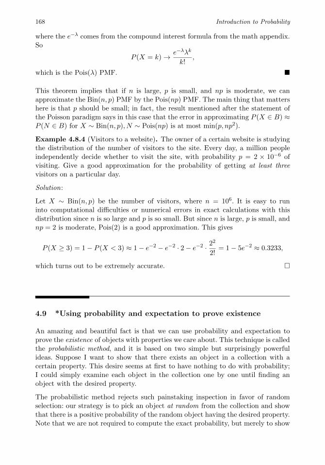
168 Introduction to Probability
where the e�� comes from the compound interest formula from the math appendix.So
P (X = k) ! e���k
k!,
which is the Pois(�) PMF. ⌅
This theorem implies that if n is large, p is small, and np is moderate, we canapproximate the Bin(n, p) PMF by the Pois(np) PMF. The main thing that mattershere is that p should be small; in fact, the result mentioned after the statement ofthe Poisson paradigm says in this case that the error in approximating P (X 2 B) ⇡P (N 2 B) for X ⇠ Bin(n, p), N ⇠ Pois(np) is at most min(p, np2).
Example 4.8.4 (Visitors to a website). The owner of a certain website is studyingthe distribution of the number of visitors to the site. Every day, a million peopleindependently decide whether to visit the site, with probability p = 2 ⇥ 10�6 ofvisiting. Give a good approximation for the probability of getting at least threevisitors on a particular day.
Solution:
Let X ⇠ Bin(n, p) be the number of visitors, where n = 106. It is easy to runinto computational di�culties or numerical errors in exact calculations with thisdistribution since n is so large and p is so small. But since n is large, p is small, andnp = 2 is moderate, Pois(2) is a good approximation. This gives
P (X � 3) = 1� P (X < 3) ⇡ 1� e�2 � e�2 · 2� e�2 · 22
2!= 1� 5e�2 ⇡ 0.3233,
which turns out to be extremely accurate. ⇤
4.9 *Using probability and expectation to prove existence
An amazing and beautiful fact is that we can use probability and expectation toprove the existence of objects with properties we care about. This technique is calledthe probabilistic method, and it is based on two simple but surprisingly powerfulideas. Suppose I want to show that there exists an object in a collection with acertain property. This desire seems at first to have nothing to do with probability;I could simply examine each object in the collection one by one until finding anobject with the desired property.
The probabilistic method rejects such painstaking inspection in favor of randomselection: our strategy is to pick an object at random from the collection and showthat there is a positive probability of the random object having the desired property.Note that we are not required to compute the exact probability, but merely to show

Expectation 169
it is greater than 0. If we can show that the probability of the property holding ispositive, then we know that there must exist an object with the property—even ifwe don’t know how to explicitly construct such an object.
Similarly, suppose each object has a score, and I want to show that there exists anobject with a “good” score—that is, a score exceeding a particular threshold. Again,we proceed by choosing a random object and considering its score,X. We know thereis an object in the collection whose score is at least E(X)—it’s impossible for everyobject to be below average! If E(X) is already a good score, then there must also bean object in the collection with a good score. Thus we can show the existence of anobject with a good score by showing that the average score is already good.
Let’s state the two key ideas formally.
• The possibility principle: Let A be the event that a randomly chosen object in acollection has a certain property. If P (A) > 0, then there exists an object withthe property.
• The good score principle: Let X be the score of a randomly chosen object. IfE(X) � c, then there is an object with a score of at least c.
To see why the possibility principle is true, consider its contrapositive: if there is noobject with the desired property, then the probability of a randomly chosen objecthaving the property is 0. Similarly, the contrapositive of the good score principle is“if all objects have a score below c, then the average score is below c”, which is truesince a weighted average of numbers less than c is a number less than c.
The probabilistic method doesn’t tell us how to find an object with the desiredproperty; it only assures us that one exists.
Example 4.9.1. A group of 100 people are assigned to 15 committees of size 20,such that each person serves on 3 committees. Show that there exist 2 committeesthat have at least 3 people in common.
Solution:
A direct approach is inadvisable here: one would have to list all possible committeeassignments and compute, for each one, the number of people in common in everypair of committees. The probabilistic method lets us bypass brute-force calculations.To prove the existence of two committees with an overlap of at least three people,we’ll calculate the average overlap of two randomly chosen committees in an arbi-trary committee assignment. So choose two committees at random, and let X bethe number of people on both committees. We can represent X = I
1
+I2
+ · · ·+I100
,where Ij = 1 if the jth person is on both committees and 0 otherwise. By symmetry,all of the indicators have the same expected value, so E(X) = 100E(I
1
), and wejust need to find E(I
1
).
By the fundamental bridge, E(I1
) is the probability that person 1 (whom we’llname Bob) is on both committees (which we’ll call A and B). There are a varietyof ways to calculate this probability; one way is to think of Bob’s committees as

170 Introduction to Probability
3 tagged elk in a population of 15. Then A and B are a sample of 2 elk, madewithout replacement. Using the HGeom(3, 12, 2) PMF, the probability that bothof these elk are tagged (i.e., the probability that both committees contain Bob) is�3
2
��12
0
�/�15
2
�= 1/35. Therefore,
E(X) = 100/35 = 20/7,
which is just shy of the desired “good score” of 3. But hope is not lost! The goodscore principle says there exist two committees with an overlap of at least 20/7, butsince the overlap between two committees must be an integer, an overlap of at least20/7 implies an overlap of at least 3. Thus, there exist two committees with at least3 people in common. ⇤
4.9.1 *Communicating over a noisy channel
Another major application of the probabilistic method is in information theory, thesubject which studies (among other things) how to achieve reliable communicationacross a noisy channel. Consider the problem of trying to send a message when thereis noise. This problem is encountered by millions of people every day, such as whentalking on the phone (you may be misheard). Suppose that the message you wantto send is represented as a binary vector x 2 {0, 1}k, and that you want to use acode to improve the chance that your message will get through successfully.
Definition 4.9.2 (Codes and rates). Given positive integers k and n, a code is afunction c that assigns to each input message x 2 {0, 1}k a codeword c(x) 2 {0, 1}n.The rate of this code is k/n (the number of input bits per output bit). After c(x)is sent, a decoder takes the received message, which may be a corrupted version ofc(x), and attempts to recover the correct x.
For example, an obvious code would be to repeat yourself a bunch of times, sendingx a bunch of times in a row, say m (with m odd); this is called a repetition code. Thereceiver could then decode by going with the majority, e.g., decoding the first bit ofx as a 1 if that bit was received more times as a 1 than as a 0. But this code may bevery ine�cient; to get the probability of failure very small, you may need to repeatyourself many times, resulting in a very low rate 1/m of communication.
Claude Shannon, the founder of information theory, showed something amazing:even in a very noisy channel, there is a code allowing for very reliable communicationat a rate that does not go to 0 as we require the probability of failure to be lower andlower. His proof was even more amazing: he studied the performance of a completelyrandom code. Richard Hamming, who worked with Shannon at Bell Labs, describedShannon’s approach as follows.
Courage is another attribute of those who do great things. Shannon is a goodexample. For some time he would come to work at about 10:00 am, play chessuntil about 2:00 pm and go home.
The important point is how he played chess. When attacked he seldom, if

Expectation 171
ever, defended his position, rather he attacked back. Such a method of playingsoon produces a very interrelated board. He would then pause a bit, think andadvance his queen saying, “I ain’t ascaird of nothin’.” It took me a while torealize that of course that is why he was able to prove the existence of goodcoding methods. Who but Shannon would think to average over all randomcodes and expect to find that the average was close to ideal? I learned fromhim to say the same to myself when stuck, and on some occasions his approachenabled me to get significant results. [16]
We will prove a version of Shannon’s result, for the case of a channel where eachtransmitted bit gets flipped (from 0 to 1 or from 1 to 0) with probability p, inde-pendently. First we need two definitions. A natural measure of distance betweenbinary vectors, named after Hamming, is as follows.
Definition 4.9.3 (Hamming distance). For two binary vectors v and w of the samelength, the Hamming distance d(v, w) is the number of positions in which they di↵er.We can write this as
d(v, w) =X
i
|vi � wi|.
The following function arises very frequently in information theory.
Definition 4.9.4 (Binary entropy function). For 0 < p < 1, the binary entropyfunction H is given by
H(p) = �p log2
p� (1� p) log2
(1� p).
We also define H(0) = H(1) = 0.
The interpretation of H(p) in information theory is that it is a measure of howmuch information we get from observing a Bern(p) r.v.; H(1/2) = 1 says that a faircoin flip provides 1 bit of information, while H(1) = 0 says that with a coin thatalways lands Heads, there’s no information gained from being told the result of theflip, since we already know the result.
Now consider a channel where each transmitted bit gets flipped with probabilityp, independently. Intuitively, it may seem that smaller p is always better, but notethat p = 1/2 is actually the worst-case scenario. In that case, technically known asa useless channel, it is impossible to send information over the channel: the outputwill be independent of the input! Analogously, in deciding whether to watch a movie,would you rather hear a review from someone you always disagree with or someoneyou agree with half the time? We now prove that for 0 < p < 1/2, it is possible tocommunicate very reliably with rate very close to 1�H(p).
Theorem 4.9.5 (Shannon). Consider a channel where each transmitted bit getsflipped with probability p, independently. Let 0 < p < 1/2 and ✏ > 0. There existsa code with rate at least 1�H(p)� ✏ that can be decoded with probability of errorless than ✏.

172 Introduction to Probability
Proof. We can assume that 1�H(p)� ✏ > 0, since otherwise there is no constrainton the rate. Let n be a large positive integer (chosen according to conditions givenbelow), and
k = dn(1�H(p)� ✏)e+ 1.
The ceiling function is there since k must be an integer. Choose p0 2 (p, 1/2) suchthat |H(p0) � H(p)| < ✏/2 (this can be done since H is continuous). We will nowstudy the performance of a random code C. To generate a random code C, we needto generate a random encoded message C(x) for all possible input messages x.
For each x 2 {0, 1}k, choose C(x) to be a uniformly random vector in {0, 1}n(making these choices independently). So we can think of C(x) as a vector consistingof n i.i.d. Bern(1/2) r.v.s. The rate k/n exceeds 1�H(p)� ✏ by definition, but let’ssee how well we can decode the received message!
Let x 2 {0, 1}k be the input message, C(x) be the encoded message, and Y 2 {0, 1}nbe the received message. For now, treat x as deterministic. But C(x) is random sincethe codewords are chosen randomly, and Y is random since C(x) is random and dueto the random noise in the channel. Intuitively, we hope that C(x) will be close toY (in Hamming distance) and C(z) will be far from Y for all z 6= x, in which case itwill be clear how to decode Y and the decoding will succeed. To make this precise,decode Y as follows:
If there exists a unique z 2 {0, 1}k such that d(C(z), Y ) np0, decode Y to that z;otherwise, declare decoder failure.
We will show that for n large enough, the probability of the decoder failing torecover the correct x is less than ✏. There are two things that could go wrong:
(a) d(C(x), Y ) > np0, or
(b) There could be some impostor z 6= x with d(C(z), Y ) np0.
Note that d(C(x), Y ) is an r.v., so d(C(x), Y ) > np0 is an event. To handle (a),represent
d(C(x), Y ) = B1
+ · · ·+Bn ⇠ Bin(n, p),
where Bi is the indicator of the ith bit being flipped. The law of large numbers (seeChapter 10) says that as n grows, the r.v. d(C(x), Y )/n will get very close to p (itsexpected value), and so will be very unlikely to exceed p0:
P (d(C(x), Y ) > np0) = P
✓B
1
+ · · ·+Bn
n> p0
◆! 0 as n ! 1.
So by choosing n large enough, we can make
P (d(C(x), Y ) > np0) < ✏/4.
To handle (b), note that d(C(z), Y ) ⇠ Bin(n, 1/2) for z 6= x, since the n bits in

Expectation 173
C(z) are i.i.d. Bern(1/2), independent of Y (to show this in more detail, conditionon Y using LOTP). Let B ⇠ Bin(n, 1/2). By Boole’s inequality,
P (d(C(z), Y ) np0 for some z 6= x) (2k � 1)P (B np0).
To simplify notation, suppose that np0 is an integer. A crude way to upper bound asum of m terms is to use m times the largest term, and a crude way to upper bounda binomial coe�cient
�nj
�is to use r�j(1 � r)�(n�j) for any r 2 (0, 1). Combining
these two crudities,
P (B np0) =1
2n
np0X
j=0
✓n
j
◆ np0 + 1
2n
✓n
np0
◆ (np0 + 1)2nH(p0
)�n,
using the fact that (p0)�np0(q0)�nq0 = 2nH(p0
) for q0 = 1� p0. Thus,
2kP (B np0) (np0 + 1)2n(1�H(p)�✏)+2+n(H(p)+✏/2)�n = 4(np0 + 1)2�n✏/2 ! 0,
so we can choose n to make P (d(C(z), Y ) np0 for some z 6= x) < ✏/4.
Assume that k and n have been chosen in accordance with the above, and let F (c, x)be the event of failure when code c is used with input message x. Putting togetherthe above results, we have shown that for a random C and any fixed x,
P (F (C, x)) < ✏/2.
It follows that for each x, there is a code c with P (F (c, x)) < ✏/2, but this is notgood enough: we want one code that works well for all x! Let X be a uniformlyrandom input message in {0, 1}k, independent of C. By LOTP, we have
P (F (C,X)) =X
x
P (F (C, x))P (X = x) < ✏/2.
Again using LOTP, but this time conditioning on C, we have
X
c
P (F (c,X))P (C = c) = P (F (C,X)) < ✏/2.
Therefore, there exists a code c such that P (F (c,X)) < ✏/2, i.e., a code c such thatthe probability of failure for a random input message X is less than ✏/2. Lastly, wewill improve c, obtaining a code that works well for all x, not just a random x. We dothis by expurgating the worst 50% of the x’s. That is, remove as legal input messagesthe 2k�1 values of x with the highest failure probabilities for code c. For all remainingx, we have P (F (c, x)) < ✏, since otherwise more than half of the x 2 {0, 1}k wouldhave more than double the average failure probability (see Markov’s inequality inChapter 10 for more about this kind of argument). By relabeling the remainingx using vectors in {0, 1}k�1, we obtain a code c0 : {0, 1}k�1 ! {0, 1}n with rate(k�1)/n � 1�H(p)� ✏ and probability less than ✏ of failure for all input messagesin {0, 1}k�1. ⌅

174 Introduction to Probability
There is also a converse to the above theorem, showing that if we require the rateto be at least 1�H(p) + ✏, it is impossible to find codes that make the probabilityof error arbitrarily small. This is why 1�H(p) is called the capacity of the channel.Shannon also obtained analogous results for much more general channels. Theseresults give theoretical bounds on what can be achieved, without saying explicitlywhich codes to use. Decades of subsequent work have been devoted to developingspecific codes that work well in practice, by coming close to the Shannon boundand allowing for e�cient encoding and decoding.
4.10 Recap
The expectation of a discrete r.v. X is
E(X) =X
x
xP (X = x).
An equivalent “ungrouped” way of calculating expectation is
E(X) =X
s
X(s)P ({s}),
where the sum is taken over pebbles in the sample space. Expectation is a singlenumber summarizing the center of mass of a distribution. A single-number summaryof the spread of a distribution is the variance, defined by
Var(X) = E(X � EX)2 = E(X2)� (EX)2.
The square root of the variance is called the standard deviation.
Expectation is linear:
E(cX) = cE(X) and E(X + Y ) = E(X) + E(Y ),
regardless of whether X and Y are independent or not. Variance is not linear:
Var(cX) = c2Var(X),
andVar(X + Y ) 6= Var(X) + Var(Y )
in general (an important exception is when X and Y are independent).
A very important strategy for calculating the expectation of a discrete r.v. X is toexpress it as a sum of indicator r.v.s, and then apply linearity and the fundamen-tal bridge. This technique is especially powerful because the indicator r.v.s neednot be independent; linearity holds even for dependent r.v.s. The strategy can besummarized in the following three steps.

Expectation 175
1. Represent the r.v. X as a sum of indicator r.v.s. To decide how to definethe indicators, think about what X is counting. For example, if X is thenumber of local maxima, as in the Putnam problem, then we should createan indicator for each local maximum that could occur.
2. Use the fundamental bridge to calculate the expected value of each indi-cator. When applicable, symmetry may be very helpful at this stage.
3. By linearity of expectation, E(X) can be obtained by adding up the ex-pectations of the indicators.
Another tool for computing expectations is LOTUS, which says we can calculate theexpectation of g(X) using only the PMF of X, via E(g(X)) =
Px g(x)P (X = x).
If g is not a linear function, it is a grave mistake to attempt to calculate E(g(X))by swapping E and g.
Three new discrete distributions to add to our list are the Geometric, NegativeBinomial, and Poisson distributions. A Geom(p) r.v. is the number of failures beforethe first success in a sequence of independent Bernoulli trials with probability p ofsuccess, and an NBin(r, p) r.v. is the number of failures before r successes. (We alsointroduced the First Success distribution, which is just a Geometric shifted so thatthe success is included.)
A Poisson r.v. is often used as an approximation for the number of successes thatoccur when there are many independent or weakly dependent trials, where eachtrial has a small probability of success. In the Binomial story, all the trials have thesame probability p of success, but in the Poisson approximation, di↵erent trials canhave di↵erent (but small) probabilities pj of success.
The Poisson, Binomial, and Hypergeometric distributions are mutually connectedvia the operations of conditioning and taking limits, as illustrated in Figure 4.8. Inthe rest of this book, we’ll continue to introduce new named distributions and addthem to this family tree, until everything is connected!
Figure 4.9 expands upon the corresponding figure from the previous chapter, furtherexploring the connections between the four fundamental objects we have considered:distributions, random variables, events, and numbers.
4.11 R
Geometric, Negative Binomial, and Poisson
The three functions for the Geometric distribution in R are dgeom, pgeom, andrgeom, corresponding to the PMF, CDF, and random number generation. For dgeom

176 Introduction to Probability
Pois
HGeom
Bin
Conditioning
Conditioning
Limit
Limit
FIGURE 4.8
Relationships between the Poisson, Binomial, and Hypergeometric.
CDF FPMF story
name, parameters
XP(X ≤ x) = F(x)
P(X = x)
func
tion o
f r.v.
X ≤ xX = x
generate
E(X), Var(X), SD(X)
X, X2, X3, …g(X)
LOTUS E(X), E(X2), E(X3), …E(g(X))
distributions random variables numbersevents
What can happen?
P
FIGURE 4.9
Four fundamental objects in probability: distributions, random variables, events,and numbers. From an r.v. X, we can generate many other r.v.s by taking functionsof X, and we can use LOTUS to find their expected values. The mean, variance,and standard deviation of X express the average and spread of the distribution ofX (in particular, they only depend on F , not directly on X itself).

Expectation 177
and pgeom, we need to supply the following as inputs: (1) the value at which toevaluate the PMF or CDF, and (2) the parameter p. For rgeom, we need to input(1) the number of random variables to generate and (2) the parameter p.
For example, to calculate P (X = 3) and P (X 3) where X ⇠ Geom(0.5), we usedgeom(3,0.5) and pgeom(3,0.5), respectively. To generate 100 i.i.d. Geom(0.8)r.v.s, we use rgeom(100,0.8). If instead we want 100 i.i.d. FS(0.8) r.v.s, we justneed to add 1 to include the success: rgeom(100,0.8)+1.
For the Negative Binomial distribution, we have dnbinom, pnbinom, and rnbinom.These take three inputs. For example, to calculate the NBin(5, 0.5) PMF at 3, wetype dnbinom(3,5,0.5).
Finally, for the Poisson distribution, the three functions are dpois, ppois, andrpois. These take two inputs. For example, to find the Pois(10) CDF at 2, we typeppois(2,10).
Matching simulation
Continuing with Example 4.4.4, let’s use simulation to calculate the expected num-ber of matches in a deck of cards. As in Chapter 1, we let n be the number of cardsin the deck and perform the experiment 104 times using replicate.
n <- 100
r <- replicate(10^4,sum(sample(n)==(1:n)))
Now r contains the number of matches from each of the 104 simulations. But insteadof looking at the probability of at least one match, as in Chapter 1, we now wantto find the expected number of matches. We can approximate this by the averageof all the simulation results, that is, the arithmetic mean of the elements of r. Thisis accomplished with the mean function:
mean(r)
The command mean(r) is equivalent to sum(r)/length(r). The result we get isvery close to 1, confirming the calculation we did in Example 4.4.4 using indicatorr.v.s. You can verify that no matter what value of n you choose, mean(r) will bevery close to 1.
Distinct birthdays simulation
Let’s calculate the expected number of distinct birthdays in a group of k people bysimulation. We’ll let k = 20, but you can choose whatever value of k you like.
k <- 20
r <- replicate(10^4,{bdays <- sample(365,k,replace=TRUE);
length(unique(bdays))})

178 Introduction to Probability
In the second line, replicate repeats the expression in the curly braces 104 times, sowe just need to understand what is inside the curly braces. First, we sample k timeswith replacement from the numbers 1 through 365 and call these the birthdays ofthe k people, bdays. Then, unique(bdays) removes duplicates in the vector bdays,and length(unique(bdays)) calculates the length of the vector after duplicateshave been removed. The two commands need to be separated by a semicolon.
Now r contains the number of distinct birthdays that we observed in each of the 104
simulations. The average number of distinct birthdays across the 104 simulationsis mean(r). We can compare the simulated value to the theoretical value that wefound in Example 4.4.5 using indicator r.v.s:
mean(r)
365*(1-(364/365)^k)
When we ran the code, both the simulated and theoretical values gave us approxi-mately 19.5.
4.12 Exercises
Expectations and variances
1. Bobo, the amoeba from Chapter 2, currently lives alone in a pond. After one minuteBobo will either die, split into two amoebas, or stay the same, with equal probability.Find the expectation and variance for the number of amoebas in the pond after oneminute.
2. In the Gregorian calendar, each year has either 365 days (a normal year) or 366 days(a leap year). A year is randomly chosen, with probability 3/4 of being a normal yearand 1/4 of being a leap year. Find the mean and variance of the number of days in thechosen year.
3. (a) A fair die is rolled. Find the expected value of the roll.
(b) Four fair dice are rolled. Find the expected total of the rolls.
4. A fair die is rolled some number of times. You can choose whether to stop after 1, 2, or3 rolls, and your decision can be based on the values that have appeared so far. Youreceive the value shown on the last roll of the die, in dollars. What is your optimalstrategy (to maximize your expected winnings)? Find the expected winnings for thisstrategy.
Hint: Start by considering a simpler version of this problem, where there are at most 2rolls. For what values of the first roll should you continue for a second roll?
5. Find the mean and variance of a Discrete Uniform r.v. on 1, 2, . . . , n.
Hint: See the math appendix for some useful facts about sums.
6. Two teams are going to play a best-of-7 match (the match will end as soon as eitherteam has won 4 games). Each game ends in a win for one team and a loss for the otherteam. Assume that each team is equally likely to win each game, and that the gamesplayed are independent. Find the mean and variance of the number of games played.
7. A certain small town, whose population consists of 100 families, has 30 families with 1child, 50 families with 2 children, and 20 families with 3 children. The birth rank of one

Expectation 179
of these children is 1 if the child is the firstborn, 2 if the child is the secondborn, and 3if the child is the thirdborn.
(a) A random family is chosen (with equal probabilities), and then a random child withinthat family is chosen (with equal probabilities). Find the PMF, mean, and variance ofthe child’s birth rank.
(b) A random child is chosen in the town (with equal probabilities). Find the PMF,mean, and variance of the child’s birth rank.
8. A certain country has four regions: North, East, South, and West. The populations ofthese regions are 3 million, 4 million, 5 million, and 8 million, respectively. There are 4cities in the North, 3 in the East, 2 in the South, and there is only 1 city in the West.Each person in the country lives in exactly one of these cities.
(a) What is the average size of a city in the country? (This is the arithmetic mean ofthe populations of the cities, and is also the expected value of the population of a citychosen uniformly at random.)
Hint: Give the cities names (labels).
(b) Show that without further information it is impossible to find the variance of thepopulation of a city chosen uniformly at random. That is, the variance depends on howthe people within each region are allocated between the cities in that region.
(c) A region of the country is chosen uniformly at random, and then a city within thatregion is chosen uniformly at random. What is the expected population size of thisrandomly chosen city?
Hint: To help organize the calculation, start by finding the PMF of the population sizeof the city.
(d) Explain intuitively why the answer to (c) is larger than the answer to (a).
9. Consider the following simplified scenario based on Who Wants to Be a Millionaire?,a game show in which the contestant answers multiple-choice questions that have 4choices per question. The contestant (Fred) has answered 9 questions correctly already,and is now being shown the 10th question. He has no idea what the right answers areto the 10th or 11th questions are. He has one “lifeline” available, which he can applyon any question, and which narrows the number of choices from 4 down to 2. Fred hasthe following options available.
(a) Walk away with $16,000.
(b) Apply his lifeline to the 10th question, and then answer it. If he gets it wrong, hewill leave with $1,000. If he gets it right, he moves on to the 11th question. He thenleaves with $32,000 if he gets the 11th question wrong, and $64,000 if he gets the11th question right.
(c) Same as the previous option, except not using his lifeline on the 10th question, andinstead applying it to the 11th question (if he gets the 10th question right).
Find the expected value of each of these options. Which option has the highest expectedvalue? Which option has the lowest variance?
10. Consider the St. Petersburg paradox (Example 4.3.13), except that you receive $n ratherthan $2n if the game lasts for n rounds. What is the fair value of this game? What ifthe payo↵ is $n2?
11. Martin has just heard about the following exciting gambling strategy: bet $1 that afair coin will land Heads. If it does, stop. If it lands Tails, double the bet for the nexttoss, now betting $2 on Heads. If it does, stop. Otherwise, double the bet for the nexttoss to $4. Continue in this way, doubling the bet each time and then stopping rightafter winning a bet. Assume that each individual bet is fair, i.e., has an expected netwinnings of 0. The idea is that
1 + 2 + 22 + 23 + · · ·+ 2n = 2n+1 � 1,

180 Introduction to Probability
so the gambler will be $1 ahead after winning a bet, and then can walk away with aprofit.
Martin decides to try out this strategy. However, he only has $31, so he may end upwalking away bankrupt rather than continuing to double his bet. On average, how muchmoney will Martin win?
12. Let X be a discrete r.v. with support �n,�n + 1, . . . , 0, . . . , n � 1, n for some positiveinteger n. Suppose that the PMF of X satisfies the symmetry property P (X = �k) =P (X = k) for all integers k. Find E(X).
13. s� Are there discrete random variables X and Y such that E(X) > 100E(Y ) but Y isgreater than X with probability at least 0.99?
14. Let X have PMF
P (X = k) = cpk/k for k = 1, 2, . . . ,
where p is a parameter with 0 < p < 1 and c is a normalizing constant. We havec = �1/ log(1� p), as seen from the Taylor series
� log(1� p) = p+p2
2+
p3
3+ . . . .
This distribution is called the Logarithmic distribution (because of the log in the aboveTaylor series), and has often been used in ecology. Find the mean and variance of X.
15. Player A chooses a random integer between 1 and 100, with probability pj of choosingj (for j = 1, 2, . . . , 100). Player B guesses the number that player A picked, and receivesthat amount in dollars if the guess is correct (and 0 otherwise).
(a) Suppose for this part that player B knows the values of pj . What is player B’soptimal strategy (to maximize expected earnings)?
(b) Show that if both players choose their numbers so that the probability of picking j isproportional to 1/j, then neither player has an incentive to change strategies, assumingthe opponent’s strategy is fixed. (In game theory terminology, this says that we havefound a Nash equilibrium.)
(c) Find the expected earnings of player B when following the strategy from (b). Expressyour answer both as a sum of simple terms and as a numerical approximation. Does thevalue depend on what strategy player A uses?
16. The dean of Blotchville University boasts that the average class size there is 20. Butthe reality experienced by the majority of students there is quite di↵erent: they findthemselves in huge courses, held in huge lecture halls, with hardly enough seats orHaribo gummi bears for everyone. The purpose of this problem is to shed light on thesituation. For simplicity, suppose that every student at Blotchville University takes onlyone course per semester.
(a) Suppose that there are 16 seminar courses, which have 10 students each, and 2 largelecture courses, which have 100 students each. Find the dean’s-eye-view average classsize (the simple average of the class sizes) and the student’s-eye-view average class size(the average class size experienced by students, as it would be reflected by surveyingstudents and asking them how big their classes are). Explain the discrepancy intuitively.
(b) Give a short proof that for any set of class sizes (not just those given above), thedean’s-eye-view average class size will be strictly less than the student’s-eye-view averageclass size, unless all classes have exactly the same size.
Hint: Relate this to the fact that variances are nonnegative.

Expectation 181
Named distributions
17. s� A couple decides to keep having children until they have at least one boy and at leastone girl, and then stop. Assume they never have twins, that the “trials” are independentwith probability 1/2 of a boy, and that they are fertile enough to keep producing childrenindefinitely. What is the expected number of children?
18. s� A coin is tossed repeatedly until it lands Heads for the first time. Let X be thenumber of tosses that are required (including the toss that landed Heads), and let pbe the probability of Heads, so that X ⇠ FS(p). Find the CDF of X, and for p = 1/2sketch its graph.
19. Let X ⇠ Bin(100, 0.9). For each of the following parts, construct an example showingthat it is possible, or explain clearly why it is impossible. In this problem, Y is a randomvariable on the same probability space as X; note that X and Y are not necessarilyindependent.
(a) Is it possible to have Y ⇠ Pois(0.01) with P (X � Y ) = 1?
(b) Is it possible to have Y ⇠ Bin(100, 0.5) with P (X � Y ) = 1?
(c) Is it possible to have Y ⇠ Bin(100, 0.5) with P (X Y ) = 1?
20. s� Alice flips a fair coin n times and Bob flips another fair coin n + 1 times, resultingin independent X ⇠ Bin(n, 1
2
) and Y ⇠ Bin(n+ 1, 1
2
).
(a) Let V = min(X,Y ) be the smaller of X and Y , and let W = max(X,Y ) be thelarger of X and Y . (If X = Y , then V = W = X = Y .) Find E(V ) + E(W ).
(b) Show that P (X < Y ) = P (n�X < n+ 1� Y ).
(c) Compute P (X < Y ). Hint: Use (b) and the fact that X and Y are integer-valued.
21. s� Raindrops are falling at an average rate of 20 drops per square inch per minute. Whatwould be a reasonable distribution to use for the number of raindrops hitting a particularregion measuring 5 inches2 in t minutes? Why? Using your chosen distribution, computethe probability that the region has no rain drops in a given 3-second time interval.
22. s� Alice and Bob have just met, and wonder whether they have a mutual friend. Eachhas 50 friends, out of 1000 other people who live in their town. They think that it’sunlikely that they have a friend in common, saying “each of us is only friends with 5%of the people here, so it would be very unlikely that our two 5%’s overlap.”
Assume that Alice’s 50 friends are a random sample of the 1000 people (equally likelyto be any 50 of the 1000), and similarly for Bob. Also assume that knowing who Alice’sfriends are gives no information about who Bob’s friends are.
(a) Compute the expected number of mutual friends Alice and Bob have.
(b) Let X be the number of mutual friends they have. Find the PMF of X.
(c) Is the distribution of X one of the important distributions we have looked at? If so,which?
23. Let X ⇠ Bin(n, p) and Y ⇠ NBin(r, p). Using a story about a sequence of Bernoullitrials, prove that P (X < r) = P (Y > n� r).
24. s� Calvin and Hobbes play a match consisting of a series of games, where Calvin hasprobability p of winning each game (independently). They play with a “win by two”rule: the first player to win two games more than his opponent wins the match. Findthe expected number of games played.
Hint: Consider the first two games as a pair, then the next two as a pair, etc.

182 Introduction to Probability
25. Nick and Penny are independently performing independent Bernoulli trials. For con-creteness, assume that Nick is flipping a nickel with probability p
1
of Heads and Pennyis flipping a penny with probability p
2
of Heads. Let X1
, X2
, . . . be Nick’s results andY1
, Y2
, . . . be Penny’s results, with Xi ⇠ Bern(p1
) and Yj ⇠ Bern(p2
).
(a) Find the distribution and expected value of the first time at which they are simul-taneously successful, i.e., the smallest n such that Xn = Yn = 1.
Hint: Define a new sequence of Bernoulli trials and use the story of the Geometric.
(b) Find the expected time until at least one has a success (including the success).
Hint: Define a new sequence of Bernoulli trials and use the story of the Geometric.
(c) For p1
= p2
, find the probability that their first successes are simultaneous, and usethis to find the probability that Nick’s first success precedes Penny’s.
26. s� Let X and Y be Pois(�) r.v.s, and T = X + Y . Suppose that X and Y are notindependent, and in fact X = Y . Prove or disprove the claim that T ⇠ Pois(2�) in thisscenario.
27. (a) Use LOTUS to show that for X ⇠ Pois(�) and any function g,
E(Xg(X)) = �E(g(X + 1)).
This is called the Stein-Chen identity for the Poisson.
(b) Find the third moment E(X3) for X ⇠ Pois(�) by using the identity from (a) and abit of algebra to reduce the calculation to the fact that X has mean � and variance �.
28. In many problems about modeling count data, it is found that values of zero in the dataare far more common than can be explained well using a Poisson model (we can makeP (X = 0) large for X ⇠ Pois(�) by making � small, but that also constrains the meanand variance of X to be small since both are �). The Zero-Inflated Poisson distributionis a modification of the Poisson to address this issue, making it easier to handle frequentzero values gracefully.
A Zero-Inflated Poisson r.v. X with parameters p and � can be generated as follows.First flip a coin with probability of p of Heads. Given that the coin lands Heads, X = 0.Given that the coin lands Tails, X is distributed Pois(�). Note that if X = 0 occurs,there are two possible explanations: the coin could have landed Heads (in which casethe zero is called a structural zero), or the coin could have landed Tails but the Poissonr.v. turned out to be zero anyway.
For example, if X is the number of chicken sandwiches consumed by a random personin a week, then X = 0 for vegetarians (this is a structural zero), but a chicken-eatercould still have X = 0 occur by chance (since they might not happen to eat any chickensandwiches that week).
(a) Find the PMF of a Zero-Inflated Poisson r.v. X.
(b) Explain why X has the same distribution as (1 � I)Y , where I ⇠ Bern(p) is inde-pendent of Y ⇠ Pois(�).
(c) Find the mean of X in two di↵erent ways: directly using the PMF of X, and usingthe representation from (b). For the latter, you can use the fact (which we prove inChapter 7) that if r.v.s Z and W are independent, then E(ZW ) = E(Z)E(W ).
(d) Find the variance X.
29. s� A discrete distribution has the memoryless property if for X a random variable withthat distribution, P (X � j + k|X � j) = P (X � k) for all nonnegative integers j, k.
(a) If X has a memoryless distribution with CDF F and PMF pi = P (X = i), find anexpression for P (X � j + k) in terms of F (j), F (k), pj , pk.
(b) Name a discrete distribution which has the memoryless property. Justify your answerwith a clear interpretation in words or with a computation.

Expectation 183
Indicator r.v.s
30. s� Randomly, k distinguishable balls are placed into n distinguishable boxes, with allpossibilities equally likely. Find the expected number of empty boxes.
31. s� A group of 50 people are comparing their birthdays (as usual, assume their birthdaysare independent, are not February 29, etc.). Find the expected number of pairs of peoplewith the same birthday, and the expected number of days in the year on which at leasttwo of these people were born.
32. s� A group of n � 4 people are comparing their birthdays (as usual, assume theirbirthdays are independent, are not February 29, etc.). Let Iij be the indicator r.v. of iand j having the same birthday (for i < j). Is I
12
independent of I34
? Is I12
independentof I
13
? Are the Iij independent?
33. s� A total of 20 bags of Haribo gummi bears are randomly distributed to 20 students.Each bag is obtained by a random student, and the outcomes of who gets which bagare independent. Find the average number of bags of gummi bears that the first threestudents get in total, and find the average number of students who get at least one bag.
34. Each of n � 2 people puts his or her name on a slip of paper (no two have the samename). The slips of paper are shu✏ed in a hat, and then each person draws one (uni-formly at random at each stage, without replacement). Find the average number ofpeople who draw their own names.
35. Two researchers independently select simple random samples from a population of sizeN , with sample sizes m and n (for each researcher, the sampling is done without re-placement, with all samples of the prescribed size equally likely). Find the expected sizeof the overlap of the two samples.
36. In a sequence of n independent fair coin tosses, what is the expected number of occur-rences of the pattern HTH (consecutively)? Note that overlap is allowed, e.g., HTHTHcontains two overlapping occurrences of the pattern.
37. You have a well-shu✏ed 52-card deck. On average, how many pairs of adjacent cardsare there such that both cards are red?
38. Suppose there are n types of toys, which you are collecting one by one. Each time youcollect a toy, it is equally likely to be any of the n types. What is the expected numberof distinct toy types that you have after you have collected t toys? (Assume that youwill definitely collect t toys, whether or not you obtain a complete set before then.)
39. A building has n floors, labeled 1, 2, . . . , n. At the first floor, k people enter the elevator,which is going up and is empty before they enter. Independently, each decides which offloors 2, 3, . . . , n to go to and presses that button (unless someone has already pressedit).
(a) Assume for this part only that the probabilities for floors 2, 3, . . . , n are equal. Findthe expected number of stops the elevator makes on floors 2, 3, . . . , n.
(b) Generalize (a) to the case that floors 2, 3, . . . , n have probabilities p2
, . . . , pn (re-spectively); you can leave your answer as a finite sum.
40. s� There are 100 shoelaces in a box. At each stage, you pick two random ends andtie them together. Either this results in a longer shoelace (if the two ends came fromdi↵erent pieces), or it results in a loop (if the two ends came from the same piece).What are the expected number of steps until everything is in loops, and the expectednumber of loops after everything is in loops? (This is a famous interview problem; leavethe latter answer as a sum.)
Hint: For each step, create an indicator r.v. for whether a loop was created then, andnote that the number of free ends goes down by 2 after each step.
41. Show that for any events A1
, . . . , An,
P (A1
\A2
· · · \An) �nX
j=1
P (Aj)� n+ 1.
184 Introduction to Probability
Hint: First prove a similar-looking statement about indicator r.v.s, by interpreting whatthe events I(A
1
\A2
· · · \An) = 1 and I(A1
\A2
· · · \An) = 0 mean.
42. You have a well-shu✏ed 52-card deck. You turn the cards face up one by one, withoutreplacement. What is the expected number of non-aces that appear before the first ace?What is the expected number between the first ace and the second ace?
43. You are being tested for psychic powers. Suppose that you do not have psychic powers.A standard deck of cards is shu✏ed, and the cards are dealt face down one by one. Justafter each card is dealt, you name any card (as your prediction). Let X be the numberof cards you predict correctly. (See Diaconis [6] for much more about the statistics oftesting for psychic powers.)
(a) Suppose that you get no feedback about your predictions. Show that no matter whatstrategy you follow, the expected value of X stays the same; find this value. (On theother hand, the variance may be very di↵erent for di↵erent strategies. For example,saying “Ace of Spades” every time gives variance 0.)
Hint: Indicator r.v.s.
(b) Now suppose that you get partial feedback: after each prediction, you are toldimmediately whether or not it is right (but without the card being revealed). Supposeyou use the following strategy: keep saying a specific card’s name (e.g., “Ace of Spades”)until you hear that you are correct. Then keep saying a di↵erent card’s name (e.g., “Twoof Spades”) until you hear that you are correct (if ever). Continue in this way, namingthe same card over and over again until you are correct and then switching to a newcard, until the deck runs out. Find the expected value of X, and show that it is veryclose to e� 1.
Hint: Indicator r.v.s.
(c) Now suppose that you get complete feedback: just after each prediction, the card isrevealed. Call a strategy “stupid” if it allows, e.g., saying “Ace of Spades” as a guessafter the Ace of Spades has already been revealed. Show that any non-stupid strategygives the same expected value for X; find this value.
Hint: Indicator r.v.s.
44. s� Let X be Hypergeometric with parameters w, b, n.
(a) Find E�X2
�by thinking, without any complicated calculations.
(b) Use (a) to find the variance of X. You should get
Var(X) =N � n
N � 1npq,
where N = w + b, p = w/N, q = 1� p.
45. There are n prizes, with values $1, $2, . . . , $n. You get to choose k random prizes,without replacement. What is the expected total value of the prizes you get?
Hint: Express the total value in the form a1
I1
+ · · ·+ anIn, where the aj are constantsand the Ij are indicator r.v.s.
46. Ten random chords of a circle are chosen, independently. To generate each of thesechords, two independent uniformly random points are chosen on the circle (intuitively,“uniformly” means that the choice is completely random, with no favoritism towardcertain angles; formally, it means that the probability of any arc is proportional to thelength of that arc). On average, how many pairs of chords intersect?
Hint: Consider two random chords. An equivalent way to generate them is to pick fourindependent uniformly random points on the circle, and then pair them up randomly.

Expectation 185
47. s� A hash table is being used to store the phone numbers of k people, storing eachperson’s phone number in a uniformly random location, represented by an integer be-tween 1 and n (see Exercise 25 from Chapter 1 for a description of hash tables). Findthe expected number of locations with no phone numbers stored, the expected numberwith exactly one phone number, and the expected number with more than one phonenumber (should these quantities add up to n?).
48. A coin with probability p of Heads is flipped n times. The sequence of outcomes canbe divided into runs (blocks of H’s or blocks of T ’s), e.g., HHHTTHTTTH becomes
HHH TT H TTTT H , which has 5 runs. Find the expected number of runs.
Hint: Start by finding the expected number of tosses (other than the first) where theoutcome is di↵erent from the previous one.
49. A population has N people, with ID numbers from 1 to N . Let yj be the value of somenumerical variable for person j, and
y =1N
NX
j=1
yj
be the population average of the quantity. For example, if yj is the height of person jthen y is the average height in the population, and if yj is 1 if person j holds a certainbelief and 0 otherwise, then y is the proportion of people in the population who hold thatbelief. In this problem, y
1
, y2
, . . . , yn are thought of as constants rather than randomvariables.
A researcher is interested in learning about y, but it is not feasible to measure yj forall j. Instead, the researcher gathers a random sample of size n, by choosing peopleone at a time, with equal probabilities at each stage and without replacement. Let Wj
be the value of the numerical variable (e.g., height) for the jth person in the sample.Even though y
1
, . . . , yn are constants, Wj is a random variable because of the randomsampling. A natural way to estimate the unknown quantity y is using
W =1n
nX
j=1
Wj .
Show that E(W ) = y in two di↵erent ways:
(a) by directly evaluating E(Wj) using symmetry;
(b) by showing that W can be expressed as a sum over the population by writing
W =1n
NX
j=1
Ijyj ,
where Ij is the indicator of person j being included in the sample, and then usinglinearity and the fundamental bridge.
50. s� Consider the following algorithm, known as bubble sort, for sorting a list of n distinctnumbers into increasing order. Initially they are in a random order, with all ordersequally likely. The algorithm compares the numbers in positions 1 and 2, and swapsthem if needed, then it compares the new numbers in positions 2 and 3, and swapsthem if needed, etc., until it has gone through the whole list. Call this one “sweep”through the list. After the first sweep, the largest number is at the end, so the secondsweep (if needed) only needs to work with the first n� 1 positions. Similarly, the thirdsweep (if needed) only needs to work with the first n � 2 positions, etc. Sweeps areperformed until n� 1 sweeps have been completed or there is a swapless sweep.
For example, if the initial list is 53241 (omitting commas), then the following 4 sweepsare performed to sort the list, with a total of 10 comparisons:
53241 ! 35241 ! 32541 ! 32451 ! 32415.

186 Introduction to Probability
32415 ! 23415 ! 23415 ! 23145.
23145 ! 23145 ! 21345.
21345 ! 12345.
(a) An inversion is a pair of numbers that are out of order (e.g., 12345 has no inversions,while 53241 has 8 inversions). Find the expected number of inversions in the originallist.
(b) Show that the expected number of comparisons is between 1
2
�n2
�and
�n2
�.
Hint: For one bound, think about how many comparisons are made if n� 1 sweeps aredone; for the other bound, use Part (a).
51. A certain basketball player practices shooting free throws over and over again. The shotsare independent, with probability p of success.
(a) In n shots, what is the expected number of streaks of 7 consecutive successful shots?(Note that, for example, 9 in a row counts as 3 streaks.)
(b) Now suppose that the player keeps shooting until making 7 shots in a row for thefirst time. Let X be the number of shots taken. Show that E(X) 7/p7.
Hint: Consider the first 7 trials as a block, then the next 7 as a block, etc.
52. s� An urn contains red, green, and blue balls. Balls are chosen randomly with replace-ment (each time, the color is noted and then the ball is put back). Let r, g, b be theprobabilities of drawing a red, green, blue ball, respectively (r + g + b = 1).
(a) Find the expected number of balls chosen before obtaining the first red ball, notincluding the red ball itself.
(b) Find the expected number of di↵erent colors of balls obtained before getting thefirst red ball.
(c) Find the probability that at least 2 of n balls drawn are red, given that at least 1 isred.
53. s� Job candidates C1
, C2
, . . . are interviewed one by one, and the interviewer comparesthem and keeps an updated list of rankings (if n candidates have been interviewed sofar, this is a list of the n candidates, from best to worst). Assume that there is no limiton the number of candidates available, that for any n the candidates C
1
, C2
, . . . , Cn areequally likely to arrive in any order, and that there are no ties in the rankings given bythe interview.
Let X be the index of the first candidate to come along who ranks as better than thevery first candidate C
1
(so CX is better than C1
, but the candidates after 1 but priorto X (if any) are worse than C
1
. For example, if C2
and C3
are worse than C1
but C4
is better than C1
, then X = 4. All 4! orderings of the first 4 candidates are equallylikely, so it could have happened that the first candidate was the best out of the first 4candidates, in which case X > 4.
What is E(X) (which is a measure of how long, on average, the interviewer needs towait to find someone better than the very first candidate)?
Hint: Find P (X > n) by interpreting what X > n says about how C1
compares withother candidates, and then apply the result of Theorem 4.4.8.
54. People are arriving at a party one at a time. While waiting for more people to arrivethey entertain themselves by comparing their birthdays. Let X be the number of peopleneeded to obtain a birthday match, i.e., before person X arrives there are no two peoplewith the same birthday, but when person X arrives there is a match.
Assume for this problem that there are 365 days in a year, all equally likely. By the

Expectation 187
result of the birthday problem from Chapter 1, for 23 people there is a 50.7% chance ofa birthday match (and for 22 people there is a less than 50% chance). But this has todo with the median of X (defined below); we also want to know the mean of X, and inthis problem we will find it, and see how it compares with 23.
(a) A median of an r.v. Y is a value m for which P (Y m) � 1/2 and P (Y �m) � 1/2 (this is also called a median of the distribution of Y ; note that the notionis completely determined by the CDF of Y ). Every distribution has a median, but forsome distributions it is not unique. Show that 23 is the unique median of X.
(b) Show that X = I1
+I2
+ · · ·+I366
, where Ij is the indicator r.v. for the event X � j.Then find E(X) in terms of pj ’s defined by p
1
= p2
= 1 and for 3 j 366,
pj =
✓1� 1
365
◆✓1� 2
365
◆. . .
✓1� j � 2
365
◆.
(c) Compute E(X) numerically. In R, the pithy command cumprod(1-(0:364)/365)
produces the vector (p2
, . . . , p366
).
(d) Find the variance of X, both in terms of the pj ’s and numerically.
Hint: What is I2i , and what is IiIj for i < j? Use this to simplify the expansion
X2 = I21
+ · · ·+ I2366
+ 2366X
j=2
j�1X
i=1
IiIj .
Note: In addition to being an entertaining game for parties, the birthday problem hasmany applications in computer science, such as in a method called the birthday attackin cryptography. It can be shown that if there are n days in a year and n is large, thenE(X) ⇡
p⇡n/2. In Volume 1 of his masterpiece The Art of Computer Programming,
Don Knuth shows that an even better approximation is
E(X) ⇡r
⇡n
2+
23+
r⇡
288n.
55. Elk dwell in a certain forest. There are N elk, of which a simple random sample of sizen is captured and tagged (so all
�Nn
�sets of n elk are equally likely). The captured elk
are returned to the population, and then a new sample is drawn. This is an importantmethod that is widely used in ecology, known as capture-recapture. If the new sampleis also a simple random sample, with some fixed size, then the number of tagged elk inthe new sample is Hypergeometric.
For this problem, assume that instead of having a fixed sample size, elk are sampledone by one without replacement until m tagged elk have been recaptured, where m isspecified in advance (of course, assume that 1 m n N). An advantage of thissampling method is that it can be used to avoid ending up with a very small numberof tagged elk (maybe even zero), which would be problematic in many applications ofcapture-recapture. A disadvantage is not knowing how large the sample will be.
(a) Find the PMFs of the number of untagged elk in the new sample (call this X) andof the total number of elk in the new sample (call this Y ).
(b) Find the expected sample size EY using symmetry, linearity, and indicator r.v.s.
Hint: We can assume that even after getting m tagged elk, they continue to be captureduntil all N of them have been obtained; briefly explain why this can be assumed. ExpressX = X
1
+ · · · + Xm, where X1
is the number of untagged elk before the first taggedelk, X
2
is the number between the first and second tagged elk, etc. Then find EXj bycreating the relevant indicator r.v. for each untagged elk in the population.

188 Introduction to Probability
(c) Suppose that m,n,N are such that EY is an integer. If the sampling is done witha fixed sample size equal to EY rather than sampling until exactly m tagged elk areobtained, find the expected number of tagged elk in the sample. Is it less than m, equalto m, or greater than m (for n < N)?
LOTUS
56. s� For X ⇠ Pois(�), find E(X!) (the average factorial of X), if it is finite.
57. For X ⇠ Pois(�), find E(2X), if it is finite.
58. For X ⇠ Geom(p), find E(2X) (if it is finite) and E(2�X) (if it is finite). For each, makesure to clearly state what the values of p are for which it is finite.
59. s� Let X ⇠ Geom(p) and let t be a constant. Find E(etX), as a function of t (this isknown as the moment generating function; we will see in Chapter 6 how this functionis useful).
60. s� The number of fish in a certain lake is a Pois(�) random variable. Worried that theremight be no fish at all, a statistician adds one fish to the lake. Let Y be the resultingnumber of fish (so Y is 1 plus a Pois(�) random variable).
(a) Find E(Y 2).
(b) Find E(1/Y ).
61. s� Let X be a Pois(�) random variable, where � is fixed but unknown. Let ✓ = e�3�,and suppose that we are interested in estimating ✓ based on the data. Since X is whatwe observe, our estimator is a function of X, call it g(X). The bias of the estimator g(X)is defined to be E(g(X))� ✓, i.e., how far o↵ the estimate is on average; the estimatoris unbiased if its bias is 0.
(a) For estimating �, the r.v. X itself is an unbiased estimator. Compute the bias of theestimator T = e�3X . Is it unbiased for estimating ✓?
(b) Show that g(X) = (�2)X is an unbiased estimator for ✓. (In fact, it turns out to bethe only unbiased estimator for ✓.)
(c) Explain intuitively why g(X) is a silly choice for estimating ✓, despite (b), and showhow to improve it by finding an estimator h(X) for ✓ that is always at least as good asg(X) and sometimes strictly better than g(X). That is,
|h(X)� ✓| |g(X)� ✓|,
with the inequality sometimes strict.
Poisson approximation
62. s� Law school courses often have assigned seating to facilitate the Socratic method.Suppose that there are 100 first-year law students, and each takes the same two courses:Torts and Contracts. Both are held in the same lecture hall (which has 100 seats), andthe seating is uniformly random and independent for the two courses.
(a) Find the probability that no one has the same seat for both courses (exactly; youshould leave your answer as a sum).
(b) Find a simple but accurate approximation to the probability that no one has thesame seat for both courses.
(c) Find a simple but accurate approximation to the probability that at least two stu-dents have the same seat for both courses.

Expectation 189
63. s� A group of n people play “Secret Santa” as follows: each puts his or her name on aslip of paper in a hat, picks a name randomly from the hat (without replacement), andthen buys a gift for that person. Unfortunately, they overlook the possibility of drawingone’s own name, so some may have to buy gifts for themselves (on the bright side, somemay like self-selected gifts better). Assume n � 2.
(a) Find the expected number of people who pick their own names.
(b) Find the expected number of pairs of people, A and B, such that A picks B’s nameand B picks A’s name (where A 6= B and order doesn’t matter).
(c) What is the approximate distribution of X if n is large (specify the parameter valueor values)? What does P (X = 0) converge to as n ! 1?
64. A survey is being conducted in a city with a million (106) people. A sample of size1000 is collected by choosing people in the city at random, with replacement and withequal probabilities for everyone in the city. Find a simple, accurate approximation tothe probability that at least one person will get chosen more than once (in contrast,Exercise 24 from Chapter 1 asks for an exact answer).
Hint: Indicator r.v.s are useful here, but creating 1 indicator for each of the millionpeople is not recommended since it leads to a messy calculation. Feel free to use thefact that 999 ⇡ 1000.
65. s� Ten million people enter a certain lottery. For each person, the chance of winning isone in ten million, independently.
(a) Find a simple, good approximation for the PMF of the number of people who winthe lottery.
(b) Congratulations! You won the lottery. However, there may be other winners. Assumenow that the number of winners other than you is W ⇠ Pois(1), and that if there ismore than one winner, then the prize is awarded to one randomly chosen winner. Giventhis information, find the probability that you win the prize (simplify).
66. Use Poisson approximations to investigate the following types of coincidences. The usualassumptions of the birthday problem apply, such as that there are 365 days in a year,with all days equally likely.
(a) How many people are needed to have a 50% chance that at least one of them hasthe same birthday as you?
(b) How many people are needed to have a 50% chance that there are two people whonot only were born on the same day, but also were born at the same hour (e.g., twopeople born between 2 pm and 3 pm are considered to have been born at the samehour).
(c) Considering that only 1/24 of pairs of people born on the same day were born at thesame hour, why isn’t the answer to (b) approximately 24 · 23? Explain this intuitively,and give a simple approximation for the factor by which the number of people neededto obtain probability p of a birthday match needs to be scaled up to obtain probabilityp of a birthday-birthhour match.
(d) With 100 people, there is a 64% chance that there are 3 with the same birthday(according to R, using pbirthday(100,classes=365,coincident=3) to compute it).Provide two di↵erent Poisson approximations for this value, one based on creating anindicator r.v. for each triplet of people, and the other based on creating an indicatorr.v. for each day of the year. Which is more accurate?
67. A chess tournament has 100 players. In the first round, they are randomly paired todetermine who plays whom (so 50 games are played). In the second round, they areagain randomly paired, independently of the first round. In both rounds, all possible

190 Introduction to Probability
pairings are equally likely. Let X be the number of people who play against the sameopponent twice.
(a) Find the expected value of X.
(b) Explain why X is not approximately Poisson.
(c) Find good approximations to P (X = 0) and P (X = 2), by thinking about games inthe second round such that the same pair played each other in the first round.
*Existence
68. s� Each of 111 people names his or her 5 favorite movies out of a list of 11 movies.
(a) Alice and Bob are 2 of the 111 people. Assume for this part only that Alice’s 5favorite movies out of the 11 are random, with all sets of 5 equally likely, and likewisefor Bob, independently. Find the expected number of movies in common to Alice’s andBob’s lists of favorite movies.
(b) Show that there are 2 movies such that at least 21 of the people name both of thesemovies as favorites.
69. s� The circumference of a circle is colored with red and blue ink such that 2/3 of thecircumference is red and 1/3 is blue. Prove that no matter how complicated the coloringscheme is, there is a way to inscribe a square in the circle such that at least three of thefour corners of the square touch red ink.
70. s� A hundred students have taken an exam consisting of 8 problems, and for eachproblem at least 65 of the students got the right answer. Show that there exist twostudents who collectively got everything right, in the sense that for each problem, atleast one of the two got it right.
71. s� Ten points in the plane are designated. You have ten circular coins (of the sameradius). Show that you can position the coins in the plane (without stacking them) sothat all ten points are covered.
Hint: Consider a honeycomb tiling of the plane (this is a way to divide the plane intohexagons). You can use the fact from geometry that if a circle is inscribed in a hexagonthen the ratio of the area of the circle to the area of the hexagon is ⇡
2
p3
> 0.9.
72. s� Let S be a set of binary strings a1
. . . an of length n (where juxtaposition meansconcatenation). We call S k-complete if for any indices 1 i
1
< · · · < ik n and anybinary string b
1
. . . bk of length k, there is a string s1
. . . sn in S such that si1
si2
. . . sik
=b1
b2
. . . bk. For example, for n = 3, the set S = {001, 010, 011, 100, 101, 110} is 2-completesince all 4 patterns of 0’s and 1’s of length 2 can be found in any 2 positions. Show thatif�nk
�2k(1� 2�k)m < 1, then there exists a k-complete set of size at most m.
Mixed practice
73. A hacker is trying to break into a password-protected website by randomly trying toguess the password. Let m be the number of possible passwords.
(a) Suppose for this part that the hacker makes random guesses (with equal probability),with replacement. Find the average number of guesses it will take until the hacker guessesthe correct password (including the successful guess).
(b) Now suppose that the hacker guesses randomly, without replacement. Find the aver-age number of guesses it will take until the hacker guesses the correct password (includingthe successful guess).
Hint: Use symmetry to find the PMF of the number of guesses.

Expectation 191
(c) Show that the answer to (a) is greater than the answer to (b) (except in the degen-erate case m = 1), and explain why this makes sense intuitively.
(d) Now suppose that the website locks out any user after n incorrect password attempts,so the hacker can guess at most n times. Find the PMF of the number of guesses thatthe hacker makes, both for the case of sampling with replacement and for the case ofsampling without replacement.
74. A fair 20-sided die is rolled repeatedly, until a gambler decides to stop. The gamblerreceives the amount shown on the die when the gambler stops. The gambler decides inadvance to roll the die until a value of m or greater is obtained, and then stop (wherem is a fixed integer with 1 m 20).
(a) What is the expected number of rolls (simplify)?
(b) What is the expected square root of the number of rolls (as a sum)?
75. s� A group of 360 people is going to be split into 120 teams of 3 (where the order ofteams and the order within a team don’t matter).
(a) How many ways are there to do this?
(b) The group consists of 180 married couples. A random split into teams of 3 is chosen,with all possible splits equally likely. Find the expected number of teams containingmarried couples.
76. s� The gambler de Mere asked Pascal whether it is more likely to get at least one six in4 rolls of a die, or to get at least one double-six in 24 rolls of a pair of dice. Continuingthis pattern, suppose that a group of n fair dice is rolled 4 · 6n�1 times.
(a) Find the expected number of times that “all sixes” is achieved (i.e., how often amongthe 4 · 6n�1 rolls it happens that all n dice land 6 simultaneously).
(b) Give a simple but accurate approximation of the probability of having at least oneoccurrence of “all sixes”, for n large (in terms of e but not n).
(c) de Mere finds it tedious to re-roll so many dice. So after one normal roll of the ndice, in going from one roll to the next, with probability 6/7 he leaves the dice in thesame configuration and with probability 1/7 he re-rolls. For example, if n = 3 and the7th roll is (3, 1, 4), then 6/7 of the time the 8th roll remains (3, 1, 4) and 1/7 of thetime the 8th roll is a new random outcome. Does the expected number of times that“all sixes” is achieved stay the same, increase, or decrease (compared with (a))? Give ashort but clear explanation.
77. s� Five people have just won a $100 prize, and are deciding how to divide the $100 upbetween them. Assume that whole dollars are used, not cents. Also, for example, giving$50 to the first person and $10 to the second is di↵erent from vice versa.
(a) How many ways are there to divide up the $100, such that each gets at least $10?
(b) Assume that the $100 is randomly divided up, with all of the possible allocationscounted in (a) equally likely. Find the expected amount of money that the first personreceives.
(c) Let Aj be the event that the jth person receives more than the first person (for2 j 5), when the $100 is randomly allocated as in (b). Are A
2
and A3
independent?
78. s� Joe’s iPod has 500 di↵erent songs, consisting of 50 albums of 10 songs each. He listensto 11 random songs on his iPod, with all songs equally likely and chosen independently(so repetitions may occur).
(a) What is the PMF of how many of the 11 songs are from his favorite album?
(b) What is the probability that there are 2 (or more) songs from the same album amongthe 11 songs he listens to?

192 Introduction to Probability
(c) A pair of songs is a match if they are from the same album. If, say, the 1st, 3rd, and7th songs are all from the same album, this counts as 3 matches. Among the 11 songshe listens to, how many matches are there on average?
79. s� In each day that the Mass Cash lottery is run in Massachusetts, 5 of the integersfrom 1 to 35 are chosen (randomly and without replacement).
(a) When playing this lottery, find the probability of guessing exactly 3 numbers right,given that you guess at least 1 of the numbers right.
(b) Find an exact expression for the expected number of days needed so that all of the�35
5
�possible lottery outcomes will have occurred.
(c) Approximate the probability that after 50 days of the lottery, every number from 1to 35 has been picked at least once.
80. The U.S. Senate consists of 100 senators, with 2 from each of the 50 states. There are dDemocrats in the Senate. A committee of size c is formed, by picking a random set ofsenators such that all sets of size c are equally likely.
(a) Find the expected number of Democrats on the committee.
(b) Find the expected number of states represented on the committee (by at least onesenator).
(c) Find the expected number of states such that both of the state’s senators are on thecommittee.
81. A certain college has g good courses and b bad courses, where g and b are positiveintegers. Alice, who is hoping to find a good course, randomly shops courses one at atime (without replacement) until she finds a good course.
(a) Find the expected number of bad courses that Alice shops before finding a goodcourse (as a simple expression in terms of g and b).
(b) Should the answer to (a) be less than, equal to, or greater than b/g? Explain thisusing properties of the Geometric distribution.
82. The Wilcoxon rank sum test is a widely used procedure for assessing whether two groupsof observations come from the same distribution. Let group 1 consist of i.i.d. X
1
, . . . , Xm
with CDF F and group 2 consist of i.i.d. Y1
, . . . , Yn with CDF G, with all of these r.v.sindependent. Assume that the probability of 2 of the observations being equal is 0 (thiswill be true if the distributions are continuous).
After the m+ n observations are obtained, they are listed in increasing order, and eachis assigned a rank between 1 and m + n: the smallest has rank 1, the second smallesthas rank 2, etc. Let Rj be the rank of Xj among all the observations for 1 j m,and let R =
Pmj=1
Rj be the sum of the ranks for group 1.
Intuitively, the Wilcoxon rank sum test is based on the idea that a very large value ofR is evidence that observations from group 1 are usually larger than observations fromgroup 2 (and vice versa if R is very small). But how large is “very large” and how smallis “very small”? Answering this precisely requires studying the distribution of the teststatistic R.
(a) The null hypothesis in this setting is that F = G. Show that if the null hypothesisis true, then E(R) = m(m+ n+ 1)/2.
(b) The power of a test is an important measure of how good the test is about sayingto reject the null hypothesis if the null hypothesis is false. To study the power of theWilcoxon rank sum stest, we need to study the distribution of R in general. So for thispart, we do not assume F = G. Let p = P (X
1
> Y1
). Find E(R) in terms of m,n, p.
Hint: Write Rj in terms of indicator r.v.s for Xj being greater than various other r.v.s.

Expectation 193
83. The legendary Caltech physicist Richard Feynman and two editors of The FeynmanLectures on Physics (Michael Gottlieb and Ralph Leighton) posed the following problemabout how to decide what to order at a restaurant. You plan to eat m meals at a certainrestaurant, where you have never eaten before. Each time, you will order one dish.
The restaurant has n dishes on the menu, with n � m. Assume that if you had triedall the dishes, you would have a definite ranking of them from 1 (your least favorite) ton (your favorite). If you knew which your favorite was, you would be happy to order italways (you never get tired of it).
Before you’ve eaten at the restaurant, this ranking is completely unknown to you. Afteryou’ve tried some dishes, you can rank those dishes amongst themselves, but don’t knowhow they compare with the dishes you haven’t yet tried. There is thus an exploration-exploitation tradeo↵ : should you try new dishes, or should you order your favorite amongthe dishes you have tried before?
A natural strategy is to have two phases in your series of visits to the restaurant: anexploration phase, where you try di↵erent dishes each time, and an exploitation phase,where you always order the best dish you obtained in the exploration phase. Let k bethe length of the exploration phase (so m� k is the length of the exploitation phase).
Your goal is to maximize the expected sum of the ranks of the dishes you eat there (therank of a dish is the “true” rank from 1 to n that you would give that dish if you couldtry all the dishes). Show that the optimal choice is
k =p
2(m+ 1)� 1,
or this rounded up or down to an integer if needed. Do this in the following steps:
(a) Let X be the rank of the best dish that you find in the exploration phase. Find theexpected sum of the ranks of the dishes you eat, in terms of E(X).
(b) Find the PMF of X, as a simple expression in terms of binomial coe�cients.
(c) Show that
E(X) =k(n+ 1)k + 1
.
Hint: Use Example 1.5.2 (about the team captain) and Exercise 18 from Chapter 1(about the hockey stick identity).
(d) Use calculus to find the optimal value of k.


5
Continuous random variables
So far we have been working with discrete random variables, whose possible valuescan be written down as a list. In this chapter we will discuss continuous r.v.s, whichcan take on any real value in an interval (possibly of infinite length, such as (0,1)or the entire real line). First we’ll look at properties of continuous r.v.s in general.Then we’ll introduce three famous continuous distributions—the Uniform, Normal,and Exponential—which, in addition to having important stories in their own right,serve as building blocks for many other useful continuous distributions.
5.1 Probability density functions
0 1 2 3 4
0.0
0.2
0.4
0.6
0.8
1.0
x
CDF
●
● ●
● ●
● ●
● ●
●
−3 −2 −1 0 1 2 3
0.0
0.2
0.4
0.6
0.8
1.0
x
CDF
FIGURE 5.1
Discrete vs. continuous r.v.s. Left: The CDF of a discrete r.v. has jumps at eachpoint in the support. Right: The CDF of a continuous r.v. increases smoothly.
Recall that for a discrete r.v., the CDF jumps at every point in the support, and isflat everywhere else. In contrast, for a continuous r.v. the CDF increases smoothly;see Figure 5.1 for a comparison of discrete vs. continuous CDFs.
Definition 5.1.1 (Continuous r.v.). An r.v. has a continuous distribution if its
195

196 Introduction to Probability
CDF is di↵erentiable. We also allow there to be endpoints (or finitely many points)where the CDF is continuous but not di↵erentiable, as long as the CDF is di↵eren-tiable everywhere else. A continuous random variable is a random variable with acontinuous distribution.
For discrete r.v.s, the CDF is awkward to work with because of its jumpiness, andits derivative is almost useless since it’s undefined at the jumps and 0 everywhereelse. But for continuous r.v.s, the CDF is often convenient to work with, and itsderivative is a very useful function, called the probability density function.
Definition 5.1.2 (Probability density function). For a continuous r.v. X with CDFF , the probability density function (PDF) of X is the derivative f of the CDF, givenby f(x) = F 0(x). The support of X, and of its distribution, is the set of all x wheref(x) > 0.
An important way in which continuous r.v.s di↵er from discrete r.v.s is that for acontinuous r.v. X, P (X = x) = 0 for all x. This is because P (X = x) is the heightof a jump in the CDF at x, but the CDF of X has no jumps! Since the PMF of acontinuous r.v. would just be 0 everywhere, we work with a PDF instead.
The PDF is analogous to the PMF in many ways, but there is a key di↵erence: fora PDF f , the quantity f(x) is not a probability, and in fact it is possible to havef(x) > 1 for some values of x. To obtain a probability, we need to integrate thePDF. The fundamental theorem of calculus tells us how to get from the PDF backto the CDF.
Proposition 5.1.3 (PDF to CDF). Let X be a continuous r.v. with PDF f . Thenthe CDF of X is given by
F (x) =
Z x
�1f(t)dt.
Proof. By the definition of PDF, F is an antiderivative of f . So by the fundamentaltheorem of calculus,
Z x
�1f(t)dt = F (x)� F (�1) = F (x).
⌅
The above result is analogous to how we obtained the value of a discrete CDF atx by summing the PMF over all values less than or equal to x; here we integratethe PDF over all values up to x, so the CDF is the accumulated area under thePDF. Since we can freely convert between the PDF and the CDF using the inverseoperations of integration and di↵erentiation, both the PDF and CDF carry completeinformation about the distribution of a continuous r.v.
Since the PDF determines the distribution, we should be able to use it to findthe probability of X falling into an interval (a, b). A handy fact is that we can

Continuous random variables 197
include or exclude the endpoints as we wish without altering the probability, sincethe endpoints have probability 0:
P (a < X < b) = P (a < X b) = P (a X < b) = P (a X b).
h 5.1.4 (Including or excluding endpoints). We can be carefree about includingor excluding endpoints as above for continuous r.v.s, but we must not be carelessabout this for discrete r.v.s.
By the definition of CDF and the fundamental theorem of calculus,
P (a < X b) = F (b)� F (a) =
Z b
af(x)dx.
Therefore, to find the probability of X falling in the interval (a, b] (or (a, b), [a, b),or [a, b]) using the PDF, we simply integrate the PDF from a to b. In general, foran arbitrary region A ✓ R,
P (X 2 A) =
Z
Af(x)dx.
In summary:
To get a desired probability, integrate the PDF over the appropriate range.
Just as a valid PMF must be nonnegative and sum to 1, a valid PDF must benonnegative and integrate to 1.
Theorem 5.1.5 (Valid PDFs). The PDF f of a continuous r.v. must satisfy thefollowing two criteria:
• Nonnegative: f(x) � 0;
• Integrates to 1:R1�1 f(x)dx = 1.
Proof. The first criterion is true because probability is nonnegative; if f(x0
) werenegative, then we could integrate over a tiny region around x
0
and get a negativeprobability. Alternatively, note that the PDF at x
0
is the slope of the CDF at x0
, sof(x
0
) < 0 would imply that the CDF is decreasing at x0
, which is not allowed. Thesecond criterion is true since
R1�1 f(x)dx is the probability of X falling somewhere
on the real line, which is 1. ⌅
Conversely, any such function f is the PDF of some r.v. This is because if f satisfiesthese properties, we can integrate it as in Proposition 5.1.3 to get a function Fsatisfying the properties of a CDF. Then a version of Universality of the Uniform,the main concept in Section 5.3, can be used to create an r.v. with CDF F .
Now let’s look at some specific examples of PDFs. The two distributions in thefollowing examples are named the Logistic and Rayleigh distributions, but we won’tdiscuss their stories here; their appearance is intended mainly as a way of gettingcomfortable with PDFs.

198 Introduction to Probability
Example 5.1.6 (Logistic). The Logistic distribution has CDF
F (x) =ex
1 + ex, x 2 R.
To get the PDF, we di↵erentiate the CDF, which gives
f(x) =ex
(1 + ex)2, x 2 R.
Let X ⇠ Logistic. To find P (�2 < X < 2), we need to integrate the PDF from �2to 2.
P (�2 < X < 2) =
Z2
�2
ex
(1 + ex)2dx = F (2)� F (�2) ⇡ 0.76.
The integral was easy to evaluate since we already knew that F was an antiderivativefor f , and we had a nice expression for F . Otherwise, we could have made thesubstitution u = 1 + ex, so du = exdx, giving
Z2
�2
ex
(1 + ex)2dx =
Z1+e2
1+e�2
1
u2du =
✓�1
u
◆ ���1+e2
1+e�2
⇡ 0.76.
Figure 5.2 shows the Logistic PDF (left) and CDF (right). On the PDF, P (�2 <X < 2) is represented by the shaded area; on the CDF, it is represented by theheight of the curly brace. You can check that the properties of a valid PDF andCDF are satisfied.
−4 −2 0 2 4
0.00
0.10
0.20
0.30
x
−4 −2 0 2 4
0.0
0.2
0.4
0.6
0.8
1.0
x
CDF
FIGURE 5.2
Logistic PDF and CDF. The probability P (�2 < X < 2) is indicated by the shadedarea under the PDF and the height of the curly brace on the CDF.
⇤

Continuous random variables 199
Example 5.1.7 (Rayleigh). The Rayleigh distribution has CDF
F (x) = 1� e�x2/2, x > 0.
To get the PDF, we di↵erentiate the CDF, which gives
f(x) = xe�x2/2, x > 0.
For x 0, both the CDF and PDF are equal to 0.
Let X ⇠ Rayleigh. To find P (X > 2), we need to integrate the PDF from 2 to 1.We can do that by making the substitution u = �x2/2, but since we already havethe CDF in a nice form we know the integral is F (1)� F (2) = 1� F (2):
P (X > 2) =
Z 1
2
xe�x2/2dx = 1� F (2) ⇡ 0.14.
The Rayleigh PDF and CDF are plotted in Figure 5.3. Again, probability is repre-sented by a shaded area on the PDF and a vertical height on the CDF. ⇤
0 1 2 3 4 5
0.0
0.2
0.4
0.6
0.8
x
0 1 2 3 4 5
0.0
0.2
0.4
0.6
0.8
1.0
x
CDF
FIGURE 5.3
Rayleigh PDF and CDF. The probability P (X > 2) is indicated by the shaded areaunder the PDF and the height of the curly brace on the CDF.
Although the height of a PDF at x does not represent a probability, it is closelyrelated to the probability of falling into a tiny interval around x, as the followingintuition explains.
Intuition 5.1.8. Let F be the CDF and f be the PDF of a continuous r.v. X. Asmentioned earlier, f(x) is not a probability; for example, we could have f(3) > 1,and we know P (X = 3) = 0. But thinking about the probability of X being veryclose to 3 gives us a way to interpret f(3). Specifically, the probability of X beingin a tiny interval of length ✏, centered at 3, will essentially be f(3)✏. This is because
P (3� ✏/2 < X < 3 + ✏/2) =
Z3+✏/2
3�✏/2f(x)dx ⇡ f(3)✏,

200 Introduction to Probability
if the interval is so tiny that f is approximately the constant f(3) on that interval.In general, we can think of f(x)dx as the probability of X being in an infinitesimallysmall interval containing x, of length dx.
In practice, X often has units in some system of measurement, such as units ofdistance, time, area, or mass. Thinking about the units is not only important inapplied problems, but also it often helps in checking that answers make sense.Suppose for concreteness that X is a length, measured in centimeters (cm). Thenf(x) = dF (x)/dx is the probability per cm at x, which explains why f(x) is a prob-ability density. Probability is a dimensionless quantity (a number without physicalunits), so the units of f(x) are cm�1. Therefore, to be able to get a probability again,we need to multiply f(x) by a length. When we do an integral such as
R5
0
f(x)dx,this is achieved by the often-forgotten dx. ⇤The definition of expectation for continuous r.v.s is similar to the definition fordiscrete r.v.s; we just replace the sum with an integral and the PMF with thePDF.
Definition 5.1.9 (Expectation of a continuous r.v.). The expected value (also calledthe expectation or mean) of a continuous r.v. X with PDF f is
E(X) =
Z 1
�1xf(x)dx.
As in the discrete case, the expectation of a continuous r.v. may or may not exist.When discussing expectations, it would be very tedious to have to add “(if it exists)”after every mention of an expectation not yet shown to exist, so we will often leavethis implicit.
The integral is taken over the entire real line, but if the support of X is not theentire real line we can just integrate over the support. The units in this definitionmake sense: if X is measured in cm, then so is E(X), since xf(x)dx has units ofcm · cm�1 · cm = cm.
With this definition, the expected value retains its interpretation as a center ofmass. As shown in Figure 5.4, using the Rayleigh PDF for illustrative purposes, theexpected value is the balancing point of the PDF, just as it was the balancing pointof the PMF in the discrete case.
Linearity of expectation holds for continuous r.v.s, as it did for discrete r.v.s (we willshow this later in Example 7.2.4). LOTUS also holds for continuous r.v.s, replacingthe sum with an integral and the PMF with the PDF:
Theorem 5.1.10 (LOTUS, continuous). If X is a continuous r.v. with PDF f andg is a function from R to R, then
E(g(X)) =
Z 1
�1g(x)f(x)dx.
We now have all the tools we need to tackle the named distributions of this chapter,starting with the Uniform distribution.
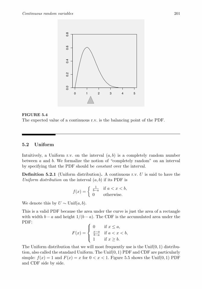
Continuous random variables 201
0 1 2 3 4 5
0.0
0.2
0.4
0.6
0.8
FIGURE 5.4
The expected value of a continuous r.v. is the balancing point of the PDF.
5.2 Uniform
Intuitively, a Uniform r.v. on the interval (a, b) is a completely random numberbetween a and b. We formalize the notion of “completely random” on an intervalby specifying that the PDF should be constant over the interval.
Definition 5.2.1 (Uniform distribution). A continuous r.v. U is said to have theUniform distribution on the interval (a, b) if its PDF is
f(x) =
⇢1
b�a if a < x < b,
0 otherwise.
We denote this by U ⇠ Unif(a, b).
This is a valid PDF because the area under the curve is just the area of a rectanglewith width b� a and height 1/(b� a). The CDF is the accumulated area under thePDF:
F (x) =
8><
>:
0 if x a,x�ab�a if a < x < b,
1 if x � b.
The Uniform distribution that we will most frequently use is the Unif(0, 1) distribu-tion, also called the standard Uniform. The Unif(0, 1) PDF and CDF are particularlysimple: f(x) = 1 and F (x) = x for 0 < x < 1. Figure 5.5 shows the Unif(0, 1) PDFand CDF side by side.
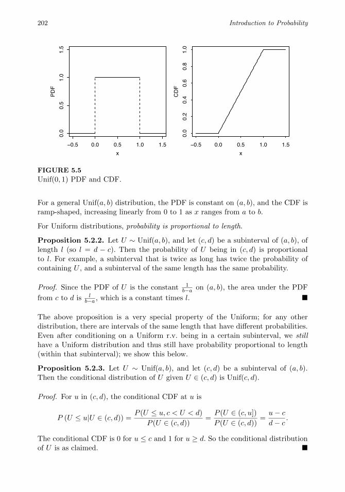
202 Introduction to Probability
−0.5 0.0 0.5 1.0 1.5
0.0
0.5
1.0
1.5
x
−0.5 0.0 0.5 1.0 1.5
0.0
0.2
0.4
0.6
0.8
1.0
x
CDF
FIGURE 5.5
Unif(0, 1) PDF and CDF.
For a general Unif(a, b) distribution, the PDF is constant on (a, b), and the CDF isramp-shaped, increasing linearly from 0 to 1 as x ranges from a to b.
For Uniform distributions, probability is proportional to length.
Proposition 5.2.2. Let U ⇠ Unif(a, b), and let (c, d) be a subinterval of (a, b), oflength l (so l = d � c). Then the probability of U being in (c, d) is proportionalto l. For example, a subinterval that is twice as long has twice the probability ofcontaining U , and a subinterval of the same length has the same probability.
Proof. Since the PDF of U is the constant 1
b�a on (a, b), the area under the PDF
from c to d is lb�a , which is a constant times l. ⌅
The above proposition is a very special property of the Uniform; for any otherdistribution, there are intervals of the same length that have di↵erent probabilities.Even after conditioning on a Uniform r.v. being in a certain subinterval, we stillhave a Uniform distribution and thus still have probability proportional to length(within that subinterval); we show this below.
Proposition 5.2.3. Let U ⇠ Unif(a, b), and let (c, d) be a subinterval of (a, b).Then the conditional distribution of U given U 2 (c, d) is Unif(c, d).
Proof. For u in (c, d), the conditional CDF at u is
P (U u|U 2 (c, d)) =P (U u, c < U < d)
P (U 2 (c, d))=
P (U 2 (c, u])
P (U 2 (c, d))=
u� c
d� c.
The conditional CDF is 0 for u c and 1 for u � d. So the conditional distributionof U is as claimed. ⌅

Continuous random variables 203
Example 5.2.4. Let’s illustrate the above propositions for U ⇠ Unif(0, 1). In thisspecial case, the support has length 1, so probability is length: the probability of Ufalling into the interval (0, 0.3) is 0.3, as is the probability of falling into (0.3, 0.6),(0.4, 0.7), or any other interval of length 0.3 within (0, 1).
Now suppose that we learn that U 2 (0.4, 0.7). Given this information, the con-ditional distribution of U is Unif(0.4, 0.7). Then the conditional probability ofU 2 (0.4, 0.6) is 2/3, since (0.4, 0.6) provides 2/3 of the length of (0.4, 0.7). Theconditional probability of U 2 (0, 0.6) is also 2/3, since we discard the points to theleft of 0.4 when conditioning on U 2 (0.4, 0.7). ⇤Next, let’s derive the mean and variance of U ⇠ Unif(a, b). The expectation isextremely intuitive: the PDF is constant, so its balancing point should be the mid-point of (a, b). This is exactly what we find by using the definition of expectationfor continuous r.v.s:
E(U) =
Z b
ax · 1
b� adx =
1
b� a
✓b2
2� a2
2
◆=
a+ b
2.
For the variance, we first find E(U2) using the continuous version of LOTUS:
E(U2) =
Z b
ax2
1
b� adx =
1
3· b
3 � a3
b� a.
Then
Var(U) = E(U2)� (EU)2 =1
3· b
3 � a3
b� a�✓a+ b
2
◆2
,
which reduces, after factoring b3�a3 = (b�a)(a2+ab+b2) and simplifying, to
Var(U) =(b� a)2
12.
The above derivation isn’t terribly painful, but there is an easier path, using atechnique that is often useful for continuous distributions. The technique is calledlocation-scale transformation, and it relies on the observation that shifting and scal-ing a Uniform r.v. produces another Uniform r.v. Shifting is considered a change oflocation and scaling is a change of scale, hence the term location-scale. For example,if X is Uniform on the interval (1, 2), then X + 5 is Uniform on the interval (6, 7),2X is Uniform on the interval (2, 4), and 2X + 5 is Uniform on (7, 9).
Definition 5.2.5 (Location-scale transformation). Let X be an r.v. and Y = �X+µ, where � and µ are constants with � > 0. Then we say that Y has been obtainedas a location-scale transformation of X. Here µ controls how the location is changedand � controls how the scale is changed.
h 5.2.6. In a location-scale transformation, starting with X ⇠ Unif(a, b) and trans-forming it to Y = cX + d where c and d are constants with c > 0, Y is a linear

204 Introduction to Probability
function of X and Uniformity is preserved: Y ⇠ Unif(ca + d, cb + d). But if Y isdefined as a nonlinear transformation of X, then Y will not be linear in general. Forexample, for X ⇠ Unif(a, b) with 0 a < b, the transformed r.v. Y = X2 has sup-port (a2, b2) but is not Uniform on that interval. Chapter 8 explores transformationsof r.v.s in detail.
In studying Uniform distributions, a useful strategy is to start with an r.v. that hasthe simplest Uniform distribution, figure things out in the friendly simple case, andthen use a location-scale transformation to handle the general case.
Let’s see how this works for finding the expectation and variance of the Unif(a, b)distribution. The location-scale strategy says to start with U ⇠ Unif(0, 1). Since thePDF of U is just 1 on the interval (0, 1), it is easy to see that
E(U) =
Z1
0
xdx =1
2,
E(U2) =
Z1
0
x2dx =1
3,
Var(U) =1
3� 1
4=
1
12.
Now that we know the answers for U , transforming U into a general Unif(a, b)r.v. takes just two steps. First we change the support from an interval of length 1to an interval of length b� a, so we multiply U by the scaling factor b� a to obtaina Unif(0, b� a) r.v. Then we shift everything until the left endpoint of the supportis at a. Thus, if U ⇠ Unif(0, 1), the random variable
U = a+ (b� a)U
is distributed Unif(a, b). Now the mean and variance of U follow directly fromproperties of expectation and variance. By linearity of expectation,
E(U) = E(a+ (b� a)U) = a+ (b� a)E(U) = a+b� a
2=
a+ b
2.
By the fact that additive constants don’t a↵ect the variance while multiplicativeconstants come out squared,
Var(U) = Var(a+ (b� a)U) = Var((b� a)U) = (b� a)2Var(U) =(b� a)2
12.
These agree with our previous answers.
The technique of location-scale transformation will work for any family of distribu-tions such that shifting and scaling an r.v. whose distribution in the family producesanother r.v. whose distribution is in the family. This technique does not apply tofamilies of discrete distributions (with a fixed support) since, for example, shiftingor scaling X ⇠ Bin(n, p) changes the support and produces an r.v. that is no longerBinomial. A Binomial r.v. must be able to take on all integer values between 0 andsome upper bound, but X + 4 can’t take on any value in {0, 1, 2, 3} and 2X canonly take even values, so neither of these r.v.s has a Binomial distribution.
Continuous random variables 205
h 5.2.7 (Beware of sympathetic magic). When using location-scale transforma-tions, the shifting and scaling should be applied to the random variables them-selves, not to their PDFs. To confuse these two would be an instance of sympa-thetic magic (see h 3.7.7), and would result in invalid PDFs. For example, letU ⇠ Unif(0, 1), so the PDF f has f(x) = 1 on (0, 1) (and f(x) = 0 elsewhere).Then 3U + 1 ⇠ Unif(1, 4), but 3f + 1 is the function that equals 4 on (0, 1) and 1elsewhere, which is not a valid PDF since it does not integrate to 1.
5.3 Universality of the Uniform
In this section, we will discuss a remarkable property of the Uniform distribution:given a Unif(0, 1) r.v., we can construct an r.v. with any continuous distribution wewant. Conversely, given an r.v. with an arbitrary continuous distribution, we cancreate a Unif(0, 1) r.v. We call this the universality of the Uniform, because it tells usthe Uniform is a universal starting point for building r.v.s with other distributions.Universality of the Uniform also goes by many other names, such as the probabilityintegral transform, inverse transform sampling, the quantile transformation, andeven the fundamental theorem of simulation.
To keep the proofs simple, we will state the universality of the Uniform for a casewhere we know that the inverse of the desired CDF exists. More generally, similarideas can be used to simulate a random draw from any desired CDF (which can beany function satisfying the properties listed in Theorem 3.6.3), as a function of aUnif(0, 1) r.v.
Theorem 5.3.1 (Universality of the Uniform). Let F be a CDF which is a continu-ous function and strictly increasing on the support of the distribution. This ensuresthat the inverse function F�1 exists, as a function from (0, 1) to R. We then havethe following results.
1. Let U ⇠ Unif(0, 1) and X = F�1(U). Then X is an r.v. with CDF F .
2. Let X be an r.v. with CDF F . Then F (X) ⇠ Unif(0, 1).
Let’s make sure we understand what each part of the theorem is saying. The firstpart of the theorem says that if we start with U ⇠ Unif(0, 1) and a CDF F , then wecan create an r.v. whose CDF is F by plugging U into the inverse CDF F�1. SinceF�1 is a function (known as the quantile function), U is a random variable, and afunction of a random variable is a random variable, F�1(U) is a random variable;universality of the Uniform says its CDF is F .
The second part of the theorem goes in the reverse direction, starting from an r.v. Xwhose CDF is F and then creating a Unif(0, 1) r.v. Again, F is a function, X is a

206 Introduction to Probability
random variable, and a function of a random variable is a random variable, so F (X)is a random variable. Since any CDF is between 0 and 1 everywhere, F (X) musttake values between 0 and 1. Universality of the Uniform says that the distributionof F (X) is Uniform on (0, 1).
h 5.3.2. The second part of universality of the Uniform involves plugging a randomvariable X into its own CDF F . This may seem strangely self-referential, but itmakes sense because F is just a function (that satisfies the properties of a validCDF), and we have already discussed in Chapter 3 what it means to take a functionof a random variable. There is a potential notational confusion, however: F (x) =P (X x) by definition, but it would be incorrect to say “F (X) = P (X X) = 1”.Rather, we should first find an expression for the CDF as a function of x, thenreplace x with X to obtain a random variable. For example, if the CDF of X isF (x) = 1� e�x for x > 0, then F (X) = 1� e�X .
Understanding the statement of the theorem is the di�cult part; the proof is just acouple of lines for each direction.
Proof.
1. Let U ⇠ Unif(0, 1) and X = F�1(U). For all real x,
P (X x) = P (F�1(U) x) = P (U F (x)) = F (x),
so the CDF of X is F , as claimed. For the last equality, we used the fact thatP (U u) = u for u 2 (0, 1).
2. Let X have CDF F , and find the CDF of Y = F (X). Since Y takes values in(0, 1), P (Y y) equals 0 for y 0 and equals 1 for y � 1. For y 2 (0, 1),
P (Y y) = P (F (X) y) = P (X F�1(y)) = F (F�1(y)) = y.
Thus Y has the Unif(0, 1) CDF. ⌅
To gain more insight into what the quantile function F�1 and universality of theUniform mean, let’s consider an example that is familiar to millions of students:percentiles on an exam.
Example 5.3.3 (Percentiles). A large number of students take a certain exam,graded on a scale from 0 to 100. Let X be the score of a random student. Con-tinuous distributions are easier to deal with here, so let’s approximate the discretedistribution of scores using a continuous distribution. Suppose that X is continuous,with a CDF F that is strictly increasing on (0, 100). In reality, there are only finitelymany students and only finitely many possible scores, but a continuous distributionmay be a good approximation.
Suppose that the median score on the exam is 60, i.e., half of the students scoreabove 60 and the other half score below 60 (a convenient aspect of assuming a

Continuous random variables 207
continuous distribution is that we don’t need to worry about how many studentshad scores equal to 60). That is, F (60) = 1/2, or, equivalently, F�1(1/2) = 60.
If Fred scores a 72 on the exam, then his percentile is the fraction of students whoscore below a 72. This is F (72), which is some number in (1/2, 1) since 72 is abovethe median. In general, a student with score x has percentile F (x). Going the otherway, if we start with a percentile, say 0.95, then F�1(0.95) is the score that hasthat percentile. A percentile is also called a quantile, which is why F�1 is calledthe quantile function. The function F converts scores to quantiles, and the functionF�1 converts quantiles to scores.
The strange operation of plugging X into its own CDF now has a natural interpre-tation: F (X) is the percentile attained by a random student. It often happens thatthe distribution of scores on an exam looks very non-Uniform. For example, thereis no reason to think that 10% of the scores are between 70 and 80, even though(70, 80) covers 10% of the range of possible scores.
On the other hand, the distribution of percentiles of the students is Uniform: theuniversality property says that F (X) ⇠ Unif(0, 1). For example, 50% of the studentshave a percentile of at least 0.5. Universality of the Uniform is expressing the factthat 10% of the students have a percentile between 0 and 0.1, 10% have a percentilebetween 0.1 and 0.2, 10% have a percentile between 0.2 and 0.3, and so on—a factthat is clear from the definition of percentile. ⇤
To illustrate universality of the Uniform, we will apply it to the two distributionswe encountered in the previous section, the Logistic and Rayleigh.
Example 5.3.4 (Universality with Logistic). The Logistic CDF is
F (x) =ex
1 + ex, x 2 R.
Suppose we have U ⇠ Unif(0, 1) and wish to generate a Logistic r.v. Part 1 of theuniversality property says that F�1(U) ⇠ Logistic, so we first invert the CDF toget F�1:
F�1(u) = log
✓u
1� u
◆.
Then we plug in U for u:
F�1(U) = log
✓U
1� U
◆.
Therefore log⇣
U1�U
⌘⇠ Logistic.
We can verify directly that log⇣
U1�U
⌘has the required CDF: start from the defini-
tion of CDF, do some algebra to isolate U on one side of the inequality, and then usethe CDF of the Uniform distribution. Let’s work through these calculations once
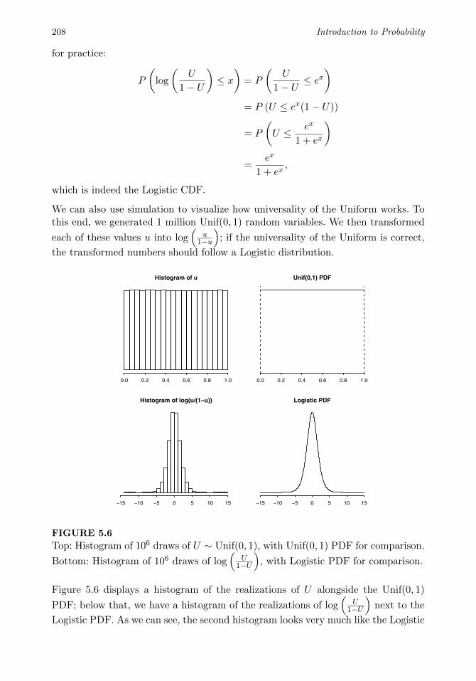
208 Introduction to Probability
for practice:
P
✓log
✓U
1� U
◆ x
◆= P
✓U
1� U ex
◆
= P (U ex(1� U))
= P
✓U ex
1 + ex
◆
=ex
1 + ex,
which is indeed the Logistic CDF.
We can also use simulation to visualize how universality of the Uniform works. Tothis end, we generated 1 million Unif(0, 1) random variables. We then transformed
each of these values u into log⇣
u1�u
⌘; if the universality of the Uniform is correct,
the transformed numbers should follow a Logistic distribution.
Histogram of u
0.0 0.2 0.4 0.6 0.8 1.0 0.0 0.2 0.4 0.6 0.8 1.0
Unif(0,1) PDF
Histogram of log(u/(1−u))
−15 −10 −5 0 5 10 15 −15 −10 −5 0 5 10 15
Logistic PDF
FIGURE 5.6
Top: Histogram of 106 draws of U ⇠ Unif(0, 1), with Unif(0, 1) PDF for comparison.
Bottom: Histogram of 106 draws of log⇣
U1�U
⌘, with Logistic PDF for comparison.
Figure 5.6 displays a histogram of the realizations of U alongside the Unif(0, 1)
PDF; below that, we have a histogram of the realizations of log⇣
U1�U
⌘next to the
Logistic PDF. As we can see, the second histogram looks very much like the Logistic
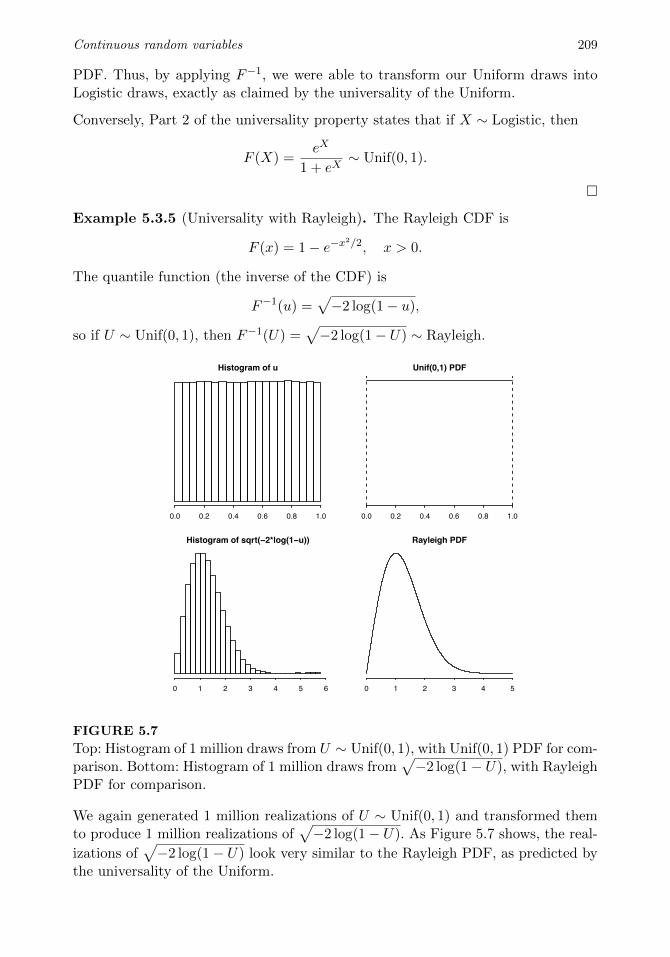
Continuous random variables 209
PDF. Thus, by applying F�1, we were able to transform our Uniform draws intoLogistic draws, exactly as claimed by the universality of the Uniform.
Conversely, Part 2 of the universality property states that if X ⇠ Logistic, then
F (X) =eX
1 + eX⇠ Unif(0, 1).
⇤Example 5.3.5 (Universality with Rayleigh). The Rayleigh CDF is
F (x) = 1� e�x2/2, x > 0.
The quantile function (the inverse of the CDF) is
F�1(u) =p
�2 log(1� u),
so if U ⇠ Unif(0, 1), then F�1(U) =p
�2 log(1� U) ⇠ Rayleigh.
Histogram of u
0.0 0.2 0.4 0.6 0.8 1.0 0.0 0.2 0.4 0.6 0.8 1.0
Unif(0,1) PDF
Histogram of sqrt(−2*log(1−u))
0 1 2 3 4 5 6 0 1 2 3 4 5
Rayleigh PDF
FIGURE 5.7
Top: Histogram of 1 million draws from U ⇠ Unif(0, 1), with Unif(0, 1) PDF for com-parison. Bottom: Histogram of 1 million draws from
p�2 log(1� U), with Rayleigh
PDF for comparison.
We again generated 1 million realizations of U ⇠ Unif(0, 1) and transformed themto produce 1 million realizations of
p�2 log(1� U). As Figure 5.7 shows, the real-
izations ofp
�2 log(1� U) look very similar to the Rayleigh PDF, as predicted bythe universality of the Uniform.

210 Introduction to Probability
Conversely, if X ⇠ Rayleigh, then F (X) = 1� e�X2/2 ⇠ Unif(0, 1). ⇤Next, let us consider the extent to which universality of the Uniform holds fordiscrete random variables. The CDF F of a discrete r.v. has jumps and flat regions,so F�1 does not exist (in the usual sense). But Part 1 still holds in the sensethat given a Uniform random variable, we can construct an r.v. with any discretedistribution we want. The di↵erence is that instead of working with the CDF, whichis not invertible, it is more straightforward to work with the PMF.
Our approach is best illustrated with a picture. Suppose we want to use U ⇠Unif(0, 1) to construct a discrete r.v. X with PMF pj = P (X = j) for j =0, 1, 2, . . . , n. As illustrated in Figure 5.8, we can chop up the interval (0, 1) intopieces of lengths p
0
, p1
, . . . , pn. By the properties of a valid PMF, the sum of thepj ’s is 1, so this perfectly divides up the interval, without overshooting or under-shooting.
p1p0 p2 pn
...pn – 1
0 1 2 n – 1 n
FIGURE 5.8
Given a PMF, chop up the interval (0, 1) into pieces, with lengths given by the PMFvalues.
Now define X to be the r.v. which equals 0 if U falls into the p0
interval, 1 if U fallsinto the p
1
interval, 2 if U falls into the p2
interval, and so on. Then X is a discreter.v. taking on values 0 through n. The probability that X = j is the probabilitythat U falls into the interval of length pj . But for a Unif(0, 1) r.v., probability islength, so P (X = j) is precisely pj , as desired!
The same trick will work for a discrete r.v. that can take on infinitely many values,such as a Poisson; we’ll need to chop (0, 1) into infinitely many pieces, but the totallength of the pieces is still 1.
We now know how to take an arbitrary PMF and create an r.v. with that PMF.This fulfills our promise from Chapter 3 that any function with the properties givenin Theorem 3.2.7 is the PMF of some r.v.
Part 2 of universality of the Uniform, on the other hand, fails for discrete r.v.s.A function of a discrete r.v. is still discrete, so if X is discrete, then F (X) is stilldiscrete. So F (X) doesn’t have a Uniform distribution. For example, ifX ⇠ Bern(p),then F (X) has only two possible values: F (0) = 1� p and F (1) = 1.
The takeaway from this section is that we can use a Uniform r.v. U generate r.v.sfrom both continuous and discrete distributions: in the continuous case, we can plugU into the inverse CDF, and in the discrete case, we can chop up the unit interval

Continuous random variables 211
according to the desired PMF. Universality of the Uniform is often useful in practicewhen running simulations (since the software being used may know how to generateUniform r.v.s but not know how to generate r.v.s with the distribution of interest),though the extent to which it is useful depends partly on how tractable it is tocompute the inverse CDF.
Using our analogy of distributions as blueprints and r.v.s as houses, the beauty ofthe universality property is that the Uniform distribution is a very simple blueprint,and it’s easy to create a house from that blueprint; universality of the Uniform thengives us a simple rule for remodeling the Uniform house into a house with any otherblueprint, no matter how complicated!
5.4 Normal
The Normal distribution is a famous continuous distribution with a bell-shapedPDF. It is extremely widely used in statistics because of a theorem, the central limittheorem, which says that under very weak assumptions, the sum of a large number ofi.i.d. random variables has an approximately Normal distribution, regardless of thedistribution of the individual r.v.s. This means we can start with independent r.v.sfrom almost any distribution, discrete or continuous, but once we add up a bunch ofthem, the distribution of the resulting r.v. looks like a Normal distribution.
The central limit theorem is a topic for Chapter 10, but in the meantime, we’llintroduce the properties of the Normal PDF and CDF and derive the expectationand variance of the Normal distribution. To do this, we will again use the strategyof location-scale transformation by starting with the simplest Normal distribution,the standard Normal, which is centered at 0 and has variance 1. After deriving theproperties of the standard Normal, we’ll be able to get to any Normal distributionwe want by shifting and scaling.
Definition 5.4.1 (Standard Normal distribution). A continuous r.v. Z is said tohave the standard Normal distribution if its PDF ' is given by
'(z) =1p2⇡
e�z2/2, �1 < z < 1.
We write this as Z ⇠ N (0, 1) since, as we will show, Z has mean 0 and variance 1.
The constant 1p2⇡
in front of the PDF may look surprising (why is something with
⇡ needed in front of something with e, when there are no circles in sight?), but it’sexactly what is needed to make the PDF integrate to 1. Such constants are callednormalizing constants because they normalize the total area under the PDF to 1.We’ll verify soon that this is a valid PDF.

212 Introduction to Probability
The standard Normal CDF � is the accumulated area under the PDF:
�(z) =
Z z
�1'(t)dt =
Z z
�1
1p2⇡
e�t2/2dt.
Some people, upon seeing the function � for the first time, express dismay that itis left in terms of an integral. Unfortunately, we have little choice in the matter:it turns out to be mathematically impossible to find a closed-form expression forthe antiderivative of ', meaning that we cannot express � as a finite sum of morefamiliar functions like polynomials or exponentials. But closed-form or no, it’s stilla well-defined function: if we give � an input z, it returns the accumulated areaunder the PDF from �1 up to z.
Notation 5.4.2. We can tell the Normal distribution must be special because thestandard Normal PDF and CDF get their own Greek letters. By convention, we use' for the standard Normal PDF and � for the CDF. We will often use Z to denotea standard Normal random variable.
The standard Normal PDF and CDF are plotted in Figure 5.9. The PDF is bell-shaped and symmetric about 0, and the CDF is S-shaped. These have the samegeneral shape as the Logistic PDF and CDF that we saw in a couple of previousexamples, but the Normal PDF decays to 0 much more quickly: notice that nearlyall of the area under ' is between �3 and 3, whereas we had to go out to �5 and5 for the Logistic PDF.
−3 −2 −1 0 1 2 3
0.0
0.1
0.2
0.3
0.4
0.5
x
−3 −2 −1 0 1 2 3
0.0
0.2
0.4
0.6
0.8
1.0
x
CDF
FIGURE 5.9
Standard Normal PDF ' (left) and CDF � (right).
There are several important symmetry properties that can be deduced from thestandard Normal PDF and CDF.
1. Symmetry of PDF : ' satisfies '(z) = '(�z), i.e., ' is an even function.

Continuous random variables 213
2. Symmetry of tail areas : The area under the PDF curve to the left of �2,which is P (Z �2) = �(�2) by definition, equals the area to the rightof 2, which is P (Z � 2) = 1� �(2). In general, we have
�(z) = 1� �(�z)
for all z. This can be seen visually by looking at the PDF curve, andmathematically by substituting u = �t below and using the fact thatPDFs integrate to 1:
�(�z) =
Z �z
�1'(t)dt =
Z 1
z'(u)du = 1�
Z z
�1'(u)du = 1� �(z).
3. Symmetry of Z and �Z: If Z ⇠ N (0, 1), then �Z ⇠ N (0, 1) as well. Tosee this, note that the CDF of �Z is
P (�Z z) = P (Z � �z) = 1� �(�z),
but that is �(z), according to what we just argued. So �Z has CDF �.
We need to prove three key facts about the standard Normal, and then we’ll beready to handle general Normal distributions: we need to show that ' is a validPDF, that E(Z) = 0, and that Var(Z) = 1.
To verify the validity of ', we’ll show that the total area under e�z2/2 isp2⇡.
However, we can’t find the antiderivative of e�z2/2 directly, again because of the an-noying fact that the antiderivative isn’t expressible in closed form. But this doesn’tmean we can’t do definite integrals, with some ingenuity.
An amazing trick saves the day here: write down the integral twice. Usually, writingdown the same problem repeatedly is more a sign of frustration than a problem-solving strategy. But in this case, it allows a neat conversion to polar coordi-nates:
✓Z 1
�1e�z2/2dz
◆✓Z 1
�1e�z2/2dz
◆=
✓Z 1
�1e�x2/2dx
◆✓Z 1
�1e�y2/2dy
◆
=
Z 1
�1
Z 1
�1e�
x
2
+y
2
2 dxdy
=
Z2⇡
0
Z 1
0
e�r2/2rdrd✓.
In the first step, we used the fact that z is just a dummy variable in each integral,so we are allowed to give it a di↵erent name (or two di↵erent names, one for eachintegral). The extra r that appears in the final step comes from the Jacobian ofthe transformation to polar coordinates, as explained in Section A.7.2 of the mathappendix. That r is also what saves us from the impossibility of the original integral,

214 Introduction to Probability
since we can now use the substitution u = r2/2, du = rdr. This gives
Z2⇡
0
Z 1
0
e�r2/2rdrd✓ =
Z2⇡
0
✓Z 1
0
e�udu
◆d✓
=
Z2⇡
0
1d✓ = 2⇡.
Therefore, Z 1
�1e�z2/2dz =
p2⇡,
as we wanted to show.
The expectation of the standard Normal has to be 0, by the symmetry of the PDF;no other balancing point would make sense. We can also see this symmetry bylooking at the definition of E(Z):
E(Z) =1p2⇡
Z 1
�1ze�z2/2dz,
and since g(z) = ze�z2/2 is an odd function (see Section A.2.3 of the math appendixfor more on even and odd functions), the area under g from �1 to 0 cancels thearea under g from 0 to 1. Therefore E(Z) = 0. In fact, the same argument showsthat E(Zn) = 0 for any odd positive number n.1
Getting the mean was easy (one might even say it was EZ), but the variancecalculation is a bit more involved. By LOTUS,
Var(Z) = E(Z2)� (EZ)2 = E(Z2)
=1p2⇡
Z 1
�1z2e�z2/2dz
=2p2⇡
Z 1
0
z2e�z2/2dz
The last step uses the fact that z2e�z2/2 is an even function. Now we use integrationby parts with u = z and dv = ze�z2/2dz, so du = dz and v = �e�z2/2:
Var(Z) =2p2⇡
✓�ze�z2/2
����1
0
+
Z 1
0
e�z2/2dz
◆
=2p2⇡
✓0 +
p2⇡
2
◆
= 1.
The first term of the integration by parts equals 0 because e�z2/2 decays much
1A subtlety is that 1�1 is undefined, so we also want to check that the area under the curve
zne�z2/2 from 0 to 1 is finite. But this is true since e�z2/2 goes to 0 extremely quickly (fasterthan exponential decay), more than o↵setting the growth of the polynomial zn.

Continuous random variables 215
faster than z grows, and the second term isp2⇡/2 because it’s half of the total area
under e�z2/2, which we’ve already proved isp2⇡. So indeed, the standard Normal
distribution has mean 0 and variance 1.
The general Normal distribution has two parameters, denoted µ and �2, whichcorrespond to the mean and variance (so the standard Normal is the special casewhere µ = 0 and �2 = 1). Starting with a standard Normal r.v. Z ⇠ N (0, 1), we canget a Normal r.v. with any mean and variance by a location-scale transformation(shifting and scaling).
Definition 5.4.3 (Normal distribution). If Z ⇠ N (0, 1), then
X = µ+ �Z
is said to have the Normal distribution with mean µ and variance �2. We denotethis by X ⇠ N (µ,�2).
It’s clear by properties of expectation and variance that X does in fact have meanµ and variance �2:
E(µ+ �Z) = E(µ) + �E(Z) = µ,
Var(µ+ �Z) = Var(�Z) = �2Var(Z) = �2.
Note that we multiply Z by the standard deviation �, not �2; else the units wouldbe wrong and X would have variance �4.
Of course, if we can get from Z to X, then we can get from X back to Z. The processof getting a standard Normal from a non-standard Normal is called, appropriatelyenough, standardization. For X ⇠ N (µ,�2), the standardized version of X is
X � µ
�⇠ N (0, 1).
We can use standardization to find the CDF and PDF of X in terms of the standardNormal CDF and PDF.
Theorem 5.4.4 (Normal CDF and PDF). Let X ⇠ N (µ,�2). Then the CDF of Xis
F (x) = �
✓x� µ
�
◆,
and the PDF of X is
f(x) = '
✓x� µ
�
◆1
�.
Proof. For the CDF, we start from the definition F (x) = P (X x), standardize,and use the CDF of the standard Normal:
F (x) = P (X x) = P
✓X � µ
� x� µ
�
◆= �
✓x� µ
�
◆.
216 Introduction to Probability
Then we di↵erentiate to get the PDF, remembering to apply the chain rule:
f(x) =d
dx�
✓x� µ
�
◆
= '
✓x� µ
�
◆1
�.
We can also write out the PDF as
f(x) =1p2⇡�
exp
✓�(x� µ)2
2�2
◆.
⌅
Finally, three important benchmarks for the Normal distribution are the probabil-ities of falling within one, two, and three standard deviations of the mean. The68-95-99.7% rule tells us that these probabilities are what the name suggests.
Theorem 5.4.5 (68-95-99.7% rule). If X ⇠ N (µ,�2), then
P (|X � µ| < �) ⇡ 0.68
P (|X � µ| < 2�) ⇡ 0.95
P (|X � µ| < 3�) ⇡ 0.997.
We can use this rule to get quick approximations of Normal probabilities.2 Often itis easier to apply the rule after standardizing, in which case we have
P (|Z| < 1) ⇡ 0.68
P (|Z| < 2) ⇡ 0.95
P (|Z| < 3) ⇡ 0.997.
Example 5.4.6. Let X ⇠ N (�1, 4). What is P (|X| < 3), exactly (in terms of �)and approximately?
Solution:
The event |X| < 3 is the same as the event �3 < X < 3. We use standardizationto express this event in terms of the standard Normal r.v. Z = (X � (�1))/2, thenapply the 68-95-99.7% rule to get an approximation. The exact answer is
P (�3 < X < 3) = P
✓�3� (�1)
2<
X � (�1)
2<
3� (�1)
2
◆= P (�1 < Z < 2),
2The 68-95-99.7% rule says that 95% of the time, a Normal random variable will fall within ±2standard deviations of its mean. An even more accurate approximation says that 95% of the time,a Normal r.v. is within ±1.96 SDs of its mean. This explains why the number 1.96 comes up veryoften in statistics in the context of 95% confidence intervals, which are often created by taking anestimate and putting a bu↵er zone of 1.96 SDs on either side.

Continuous random variables 217
which is �(2) � �(�1). The 68-95-99.7% rule tells us that P (�1 < Z < 1) ⇡ 0.68and P (�2 < Z < 2) ⇡ 0.95. In other words, going from ±1 standard deviation to±2 standard deviations adds approximately 0.95 � 0.68 = 0.27 to the area underthe curve. By symmetry, this is evenly divided between the areas P (�2 < Z < �1)and P (1 < Z < 2). Therefore,
P (�1 < Z < 2) = P (�1 < Z < 1) + P (1 < Z < 2) ⇡ 0.68 +0.27
2= 0.815.
This is close to the correct value, �(2)� �(�1) ⇡ 0.8186. ⇤
5.5 Exponential
The Exponential distribution is the continuous counterpart to the Geometric dis-tribution. Recall that a Geometric random variable counts the number of failuresbefore the first success in a sequence of Bernoulli trials. The story of the Exponen-tial distribution is analogous, but we are now waiting for a success in continuoustime, where successes arrive at a rate of � successes per unit of time. The averagenumber of successes in a time interval of length t is �t, though the actual number ofsuccesses varies randomly. An Exponential random variable represents the waitingtime until the first arrival of a success.
Definition 5.5.1 (Exponential distribution). A continuous r.v. X is said to havethe Exponential distribution with parameter � if its PDF is
f(x) = �e��x, x > 0.
We denote this by X ⇠ Expo(�).
The corresponding CDF is
F (x) = 1� e��x, x > 0.
The Expo(1) PDF and CDF are plotted in Figure 5.10. Note the resemblance tothe Geometric PMF and CDF pictured in Chapter 4. Exercise 45 explores thesense in which the Geometric converges to the Exponential, in the limit where theBernoulli trials are performed faster and faster but with smaller and smaller successprobabilities.
We’ve seen how all Uniform and Normal distributions are related to one anothervia location-scale transformations, and we might wonder whether the Exponentialdistribution allows this too. Exponential r.v.s are defined to have support (0,1),and shifting would change the left endpoint. But scale transformations work nicely,

218 Introduction to Probability
0.0 0.5 1.0 1.5 2.0 2.5 3.0
0.0
0.2
0.4
0.6
0.8
1.0
1.2
x
0.0 0.5 1.0 1.5 2.0 2.5 3.0
0.0
0.2
0.4
0.6
0.8
1.0
x
CDF
FIGURE 5.10
Expo(1) PDF and CDF.
and we can use scaling to get from the simple Expo(1) to the general Expo(�): ifX ⇠ Expo(1), then
Y =X
�⇠ Expo(�),
since
P (Y y) = P
✓X
� y
◆= P (X �y) = 1� e��y, y > 0.
Conversely, if Y ⇠ Expo(�), then �Y ⇠ Expo(1).
This means that just as we did for the Uniform and the Normal, we can get the meanand variance of the Exponential distribution by starting with X ⇠ Expo(1). BothE(X) and Var(X) are obtained using standard integration by parts calculations.This gives
E(X) =
Z 1
0
xe�xdx = 1,
E(X2) =
Z 1
0
x2e�xdx = 2,
Var(X) = E(X2)� (EX)2 = 1.
In the next chapter we’ll introduce a new tool called the moment generating func-tion, which will let us get these results without integration.
For Y = X/� ⇠ Expo(�) we then have
E(Y ) =1
�E(X) =
1
�,
Var(Y ) =1
�2Var(X) =
1
�2,

Continuous random variables 219
so the mean and variance of the Expo(�) distribution are 1/� and 1/�2, respectively.As we’d expect intuitively, the faster the rate of arrivals �, the shorter the averagewaiting time.
The Exponential distribution has a very special property called the memorylessproperty, which says that even if you’ve waited for hours or days without success,the success isn’t any more likely to arrive soon. In fact, you might as well have juststarted waiting 10 seconds ago. The definition formalizes this idea.
Definition 5.5.2 (Memoryless property). A distribution is said to have the mem-oryless property if a random variable X from that distribution satisfies
P (X � s+ t|X � s) = P (X � t)
for all s, t > 0.
Here s represents the time you’ve already spent waiting; the definition says thatafter you’ve waited s minutes, the probability you’ll have to wait another t minutesis exactly the same as the probability of having to wait t minutes with no previouswaiting time under your belt. Another way to state the memoryless property is thatconditional on X � s, the additional waiting time X�s is still distributed Expo(�).In particular, this implies
E(X|X � s) = s+ E(X) = s+1
�.
(Conditional expectation is explained in detail in Chapter 9, but the meaning shouldalready be clear: for any r.v. X and event A, E(X|A) is the expected value of Xgiven A; this can be defined by replacing the unconditional PMF or PDF of X inthe definition of E(X) by the conditional PMF or PDF of X given A.)
Using the definition of conditional probability, we can directly verify that the Ex-ponential distribution has the memoryless property. Let X ⇠ Expo(�). Then
P (X � s+ t|X � s) =P (X � s+ t)
P (X � s)=
e��(s+t)
e��s= e��t = P (X � t).
What are the implications of the memoryless property? If you’re waiting at a busstop and the time until the bus arrives has an Exponential distribution, then con-ditional on your having waited 30 minutes, the bus isn’t due to arrive soon. Thedistribution simply forgets that you’ve been waiting for half an hour, and your re-maining wait time is the same as if you had just shown up to the bus stop. If thelifetime of a machine has an Exponential distribution, then no matter how long themachine has been functional, conditional on having lived that long, the machineis as good as new: there is no wear-and-tear e↵ect that makes the machine morelikely to break down soon. If human lifetimes were Exponential, then conditionalon having survived to the age of 80, your remaining lifetime would have the samedistribution as that of a newborn baby!
Clearly, the memoryless property is not an appropriate description for human ormachine lifetimes. Why then do we care about the Exponential distribution?

220 Introduction to Probability
1. Some physical phenomena, such as radioactive decay, truly do exhibit thememoryless property, so the Exponential is an important model in its ownright.
2. The Exponential distribution is well-connected to other named distribu-tions. In the next section, we’ll see how the Exponential and Poisson dis-tributions can be united by a shared story, and we’ll discover many moreconnections in later chapters.
3. The Exponential serves as a building block for more flexible distributions,such as the Weibull distribution (see Exercise 25 of Chapter 6), that allowfor a wear-and-tear e↵ect (where older units are due to break down) ora survival-of-the-fittest e↵ect (where the longer you’ve lived, the strongeryou get). To understand these distributions, we first have to understandthe Exponential.
The memoryless property is a very special property of the Exponential distribu-tion: no other continuous distribution on (0,1) is memoryless! Let’s prove thisnow.
Theorem 5.5.3. IfX is a positive continuous random variable with the memorylessproperty, then X has an Exponential distribution.
Proof. Suppose X is a positive continuous r.v. with the memoryless property. LetF be the CDF of X, and let G(x) = P (X > x) = 1 � F (x); G is known as thesurvival function. We’re going to show thatG(x) = e��x for some �. The memorylessproperty says
G(s+ t) = G(s)G(t)
for all s, t > 0. Di↵erentiating with respect to s (which we can do because X is acontinuous r.v., so G is di↵erentiable), we require
G0(s+ t) = G0(s)G(t)
for all s, t > 0. In particular, when s = 0,
G0(t) = G0(0)G(t).
Let G0(0) = c, since it’s just a number, and let y = G(t). Then what we have is aseparable di↵erential equation (see Section A.5 of the math appendix),
dy
dt= cy,
which has general solution y = G(t) = Kect and particular solution G(t) = ect
after using the initial condition G(0) = P (X > 0) = 1. Letting � = �c, this isexactly the form we wanted for G(t); � is indeed positive because G is a decreasingfunction (since F is an increasing function), so c = G0(0) < 0. Therefore X has anExponential distribution. ⌅

Continuous random variables 221
In view of the analogy between the Geometric and Exponential stories, you mightguess that the Geometric distribution also has the memoryless property. If so, youwould be correct! If we’re waiting for the first Heads in a sequence of fair coin tosses,and in a streak of bad luck we happen to get ten Tails in a row, this has no impact onhow many additional tosses we’ll need: the coin isn’t due for a Heads, nor conspiringagainst us to perpetually land Tails. The coin is memoryless. The Geometric is theonly memoryless discrete distribution (with support 0, 1, . . . ), and the Exponentialis the only memoryless continuous distribution (with support (0,1)).
As practice with the memoryless property, the following example chronicles the ad-ventures of Fred, who experiences firsthand the frustrations of the memoryless prop-erty after moving to a town with a memoryless public transportation system.
Example 5.5.4 (Blissville and Blotchville). Fred lives in Blissville, where busesalways arrive exactly on time, with the time between successive buses fixed at 10minutes. Having lost his watch, he arrives at the bus stop at a uniformly randomtime on a certain day (assume that buses run 24 hours a day, every day, and thatthe time that Fred arrives is independent of the bus arrival process).
(a) What is the distribution of how long Fred has to wait for the next bus? Whatis the average time that Fred has to wait?
(b) Given that the bus has not yet arrived after 6 minutes, what is the probabilitythat Fred will have to wait at least 3 more minutes?
(c) Fred moves to Blotchville, a city with inferior urban planning and where busesare much more erratic. Now, when any bus arrives, the time until the next busarrives is an Exponential random variable with mean 10 minutes. Fred arrives atthe bus stop at a random time, not knowing how long ago the previous bus came.What is the distribution of Fred’s waiting time for the next bus? What is the averagetime that Fred has to wait?
(d) When Fred complains to a friend how much worse transportation is inBlotchville, the friend says: “Stop whining so much! You arrive at a uniform in-stant between the previous bus arrival and the next bus arrival. The average lengthof that interval between buses is 10 minutes, but since you are equally likely toarrive at any time in that interval, your average waiting time is only 5 minutes.”
Fred disagrees, both from experience and from solving Part (c) while waiting forthe bus. Explain what is wrong with the friend’s reasoning.
Solution:
(a) The distribution is Uniform on (0, 10), so the mean is 5 minutes.
(b) Let T be the waiting time. Then
P (T � 6 + 3|T > 6) =P (T � 9, T > 6)
P (T > 6)=
P (T � 9)
P (T > 6)=
1/10
4/10=
1
4.
In particular, Fred’s waiting time in Blissville is not memoryless; conditional on

222 Introduction to Probability
having waited 6 minutes already, there’s only a 1/4 chance that he’ll have to waitanother 3 minutes, whereas if he had just showed up, there would be a P (T � 3) =7/10 chance of having to wait at least 3 minutes.
(c) By the memoryless property, the distribution is Exponential with parameter1/10 (and mean 10 minutes) regardless of when Fred arrives; how much longer thenext bus will take to arrive is independent of how long ago the previous bus arrived.The average time that Fred has to wait is 10 minutes.
(d) Fred’s friend is making the mistake, explained in h 4.1.3, of replacing a randomvariable (the time between buses) by its expectation (10 minutes), thereby ignoringthe variability in interarrival times. The average length of a time interval betweentwo buses is 10 minutes, but Fred is not equally likely to arrive at any of theseintervals: Fred is more likely to arrive during a long interval between buses than toarrive during a short interval between buses. For example, if one interval betweenbuses is 50 minutes and another interval is 5 minutes, then Fred is 10 times morelikely to arrive during the 50-minute interval.
This phenomenon is known as length-biasing, and it comes up in many real-lifesituations. For example, asking randomly chosen mothers how many children theyhave yields a di↵erent distribution from asking randomly chosen people how manysiblings they have, including themselves. Asking students the sizes of their classesand averaging those results may give a much higher value than taking a list of classesand averaging the sizes of each (this is called the class size paradox ).
Fred’s adventures in Blissville and Blotchville continue in the exercises. See alsoMacKay [18] for more of Fred’s adventures. ⇤
5.6 Poisson processes
The Exponential distribution is closely connected to the Poisson distribution, assuggested by our use of � for the parameters of both distributions. In this sectionwe will see that the Exponential and Poisson are linked by a common story, whichis the story of the Poisson process. A Poisson process is a sequence of arrivalsoccurring at di↵erent points on a timeline, such that the number of arrivals in aparticular interval of time has a Poisson distribution. Poisson processes are discussedin much greater detail in Chapter 13, but we already have the tools to understandthe definition and basic properties.
Definition 5.6.1 (Poisson process). A process of arrivals in continuous time iscalled a Poisson process with rate � if the following two conditions hold.
1. The number of arrivals that occur in an interval of length t is a Pois(�t)random variable.

Continuous random variables 223
2. The numbers of arrivals that occur in disjoint intervals are indepen-dent of each other. For example, the numbers of arrivals in the intervals(0, 10), [10, 12), and [15,1) are independent.
A sketch of a Poisson process is pictured in Figure 5.11. Each X marks the spot ofan arrival.
0 T1 T2 T3 T4 T5
+ + + + +
FIGURE 5.11
Poisson process.
For concreteness, suppose the arrivals are emails landing in an inbox according toa Poisson process with rate �. There are several things we might want to knowabout this process. One question we could ask is: in one hour, how many emailswill arrive? The answer comes directly from the definition, which tells us that thenumber of emails in an hour follows a Pois(�) distribution. Notice that the numberof emails is a nonnegative integer, so a discrete distribution is appropriate.
But we could also flip the question around and ask: how long does it take until thefirst email arrives (measured relative to some fixed starting point)? The waiting timefor the first email is a positive real number, so a continuous distribution on (0,1) isappropriate. Let T
1
be the time until the first email arrives. To find the distributionof T
1
, we just need to understand one crucial fact: saying that the waiting time forthe first email is greater than t is the same as saying that no emails have arrivedbetween 0 and t. In other words, if Nt is the number of emails that arrive at orbefore time t, then
T1
> t is the same event as Nt = 0.
We call this the count-time duality because it connects a discrete r.v., Nt, whichcounts the number of arrivals, with a continuous r.v., T
1
, which marks the time ofthe first arrival.
If two events are the same, they have the same probability. Since Nt ⇠ Pois(�t) bythe definition of Poisson process,
P (T1
> t) = P (Nt = 0) =e��t(�t)0
0!= e��t.
Therefore P (T1
t) = 1� e��t, so T1
⇠ Expo(�)! The time until the first arrival ina Poisson process of rate � has an Exponential distribution with parameter �.
What about T2
� T1
, the time between the first and second arrivals? Since disjointintervals in a Poisson process are independent by definition, the past is irrelevant

224 Introduction to Probability
once the first arrival occurs. Thus T2
� T1
is independent of the time until thefirst arrival, and by the same argument as before, T
2
� T1
also has an Exponentialdistribution with rate �.
Similarly, T3
� T2
⇠ Expo(�) independently of T1
and T2
� T1
. Continuing in thisway, we deduce that all the interarrival times are i.i.d. Expo(�) random variables.To summarize what we’ve learned: in a Poisson process of rate �,
• the number of arrivals in an interval of length 1 is Pois(�), and
• the times between arrivals are i.i.d. Expo(�).
Thus, Poisson processes tie together two important distributions, one discrete andone continuous, and the use of a common symbol � for both the Poisson and Expo-nential parameters is felicitous notation, for � is the arrival rate in the process thatunites the two distributions.
h 5.6.2. The total time until the second arrival, T2
, is the sum of two independentExpo(�) r.v.s, T
1
and T2
� T1
. This is not an Exponential distribution, but rathera Gamma distribution, which is introduced in Chapter 8.
The story of the Poisson process provides intuition for the fact that the minimumof independent Exponential r.v.s is another Exponential r.v.
Example 5.6.3 (Minimum of independent Expos). LetX1
, . . . , Xn be independent,with Xj ⇠ Expo(�j). Let L = min(X
1
, . . . , Xn). Show that L ⇠ Expo(�1
+ · · ·+�n),and interpret this intuitively.
Solution:
We can find the distribution of L by considering its survival function P (L > t),since the survival function is 1 minus the CDF.
P (L > t) = P (min(X1
, . . . , Xn) > t) = P (X1
> t, . . . , Xn > t)
= P (X1
> t) · · ·P (Xn > t) = e��1
t · · · e��n
t = e�(�1
+···+�n
)t.
The second equality holds since saying that the minimum of the Xj is greater thant is the same as saying that all of the Xj are greater than t. The third equality holdsby independence of the Xj . Thus, L has the survival function (and the CDF) of anExponential distribution with parameter �
1
+ · · ·+ �n.
Intuitively, we can interpret the �j as the rates of n independent Poisson processes.We can imagine, for example, X
1
as the waiting time for a green car to pass by, X2
as the waiting time for a blue car to pass by, and so on, assigning a color to eachXj . Then L is the waiting time for a car with any of these colors to pass by, so itmakes sense that L has a combined rate of �
1
+ · · ·+ �n. ⇤

Continuous random variables 225
5.7 Symmetry of i.i.d. continuous r.v.s
Continuous r.v.s that are independent and identically distributed have an importantsymmetry property: all possible rankings are equally likely.
Proposition 5.7.1. Let X1
, . . . , Xn be i.i.d. from a continuous distribution. ThenP (Xa
1
< · · · < Xan
) = 1/n! for any permutation a1
, . . . , an of 1, . . . , n.
Proof. Let F be the CDF of Xj . By symmetry, all orderings of X1
, . . . , Xn areequally likely. For example, P (X
3
< X2
< X1
) = P (X1
< X2
< X3
) since bothsides have exactly the same structure: they are both of the form P (A < B < C)where A,B,C are i.i.d. draws from F . For any i and j with i 6= j, the probabilityof the tie Xi = Xj is 0 since Xi and Xj are independent continuous r.v.s. So theprobability of there being at least one tie among X
1
, . . . , Xn is also 0, since
P
0
@[
i 6=j
{Xi = Xj}
1
A X
i 6=j
P (Xi = Xj) = 0.
Thus, X1
, . . . , Xn are distinct with probability 1, and the probability of any partic-ular ordering is 1/n!. ⌅
h 5.7.2. The proposition may fail if the r.v.s are dependent. Let n = 2, andconsider the extreme case where X
1
and X2
are so dependent that they are alwaysequal, i.e., X
1
= X2
with probability 1. Then P (X1
< X2
) = P (X2
< X1
) = 0. Fordependent X
1
, X2
we can also make P (X1
< X2
) 6= P (X2
< X1
). For an example,see Exercise 42 from Chapter 3.
For example, if X and Y are i.i.d. continuous r.v.s, then P (X < Y ) = P (Y < X) =1/2 by symmetry and since the probability of a tie is 0: P (X = Y ) = 0. If X andY are i.i.d. discrete r.v.s, it is still true that P (X < Y ) = P (Y < X) by symmetry,but this number is less than 1/2 because of the possibility of a tie.
The ranks of a list of distinct numbers are defined by giving the smallest numbera rank of 1, the second smallest a rank of 2, and so on. For example, the ranks for3.14, 2.72, 1.41, 1.62 are 4, 3, 1, 2. The proposition says that the ranks of i.i.d. con-tinuous X
1
, . . . , Xn are a uniformly random permutation of the numbers 1, . . . , n.The next example shows how we can use this symmetry property in conjunctionwith indicator r.v.s in problems involving records, such as the record level of rainfallor the record performance on a high jump.
Example 5.7.3 (Records). Athletes compete one at a time at the high jump. LetXj be how high the jth jumper jumped, with X
1
, X2
, . . . i.i.d. with a continuousdistribution. We say that the jth jumper sets a record if Xj is greater than all ofXj�1
, . . . , X1
.

226 Introduction to Probability
(a) Is the event “the 110th jumper sets a record” independent of the event “the111th jumper sets a record”?
(b) Find the mean number of records among the first n jumpers. What happens tothe mean as n ! 1?
(c) A double record occurs at time j if both the jth and (j�1)st jumpers set records.Find the mean number of double records among the first n jumpers. What happensto the mean as n ! 1?
Solution:
(a) Let Ij be the indicator r.v. for the jth jumper setting a record. By symmetry,P (Ij = 1) = 1/j (as any of the first j jumps is equally likely to be the highest ofthose jumps). Also,
P (I110
= 1, I111
= 1) =109!
111!=
1
110 · 111 ,
since in order for both the 110th and 111th jumps to be records, we need the highestof the first 111 jumps to be in position 111 and the second highest to be in position110, and the remaining 109 can be in any order. So
P (I110
= 1, I111
= 1) = P (I110
= 1)P (I111
= 1),
which shows that the 110th jumper setting a record is independent of the 111thjumper setting a record. Intuitively, this makes sense since learning that the 111thjumper sets a record gives us no information about the “internal” matter of howthe first 110 jumps are arranged amongst themselves.
(b) By linearity, the expected number of records among the first n jumpers isPnj=1
1
j , which goes to 1 as n ! 1 since the harmonic series diverges.
(c) Let Jj be the indicator r.v. for a double record occurring at time j, for 2 j n.Then P (Jj = 1) = 1
j(j�1)
, following the logic of part (a). So the expected numberof double records is
nX
j=2
1
j(j � 1)=
nX
j=2
✓1
j � 1� 1
j
◆= 1� 1
n,
since all the other terms cancel out. Thus, the expected number of records goes to1 as n ! 1, but the expected number of double records goes to 1. ⇤
5.8 Recap
A continuous r.v. can take on any value in an interval, although the probabilitythat it equals any particular value is exactly 0. The CDF of a continuous r.v. is

Continuous random variables 227
di↵erentiable, and the derivative is called the probability density function (PDF).Probability is represented by area under the PDF curve, not by the value of thePDF at a point. We must integrate the PDF to get a probability. The table belowsummarizes and compares some important concepts in the discrete case and thecontinuous case.
Discrete r.v. Continuous r.v.
CDF F (x) = P (X x) F (x) = P (X x)
PMF/PDF P (X = x) is height of jump of F at x
• PMF is nonnegative and sums to 1:P
x P (X = x) = 1.
• To get probability of X being in some set, sumPMF over that set.
f(x) = dF (x)dx
• PDF is nonnegative and integrates to 1:R1�1 f(x)dx = 1.
• To get probability of X being in some region, in-tegrate PDF over that region.
Expectation E(X) =X
x
xP (X = x) E(X) =
Z 1
�1xf(x)dx
LOTUS E(g(X)) =X
x
g(x)P (X = x) E(g(X)) =
Z 1
�1g(x)f(x)dx
Three important continuous distributions are the Uniform, Normal, and Exponen-tial. A Unif(a, b) r.v. is a “completely random” number in the interval (a, b), and ithas the property that probability is proportional to length. The universality of theUniform tells us how we can use a Unif(0, 1) r.v. to construct r.v.s from other dis-tributions we may be interested in; it also says that if we plug a continuous r.v. intoits own CDF, the resulting r.v. has a Unif(0, 1) distribution.
A N (µ,�2) r.v. has a symmetric bell-shaped PDF centered at µ, with � controllinghow spread out the curve is. The mean is µ and standard deviation is �. The 68-95-99.7% rule gives important benchmarks for the probability of a Normal r.v. fallingwithin 1, 2, and 3 standard deviations of its mean.
An Expo(�) r.v. represents the waiting time for the first success in continuous time,analogous to how a Geometric r.v. represents the number of failures before the firstsuccess in discrete time; the parameter � can be interpreted as the rate at whichsuccesses arrive. The Exponential distribution has the memoryless property, whichsays that conditional on our having waited a certain amount of time without success,the distribution of the remaining wait time is exactly the same as if we hadn’t waitedat all. In fact, the Exponential is the only positive continuous distribution with thememoryless property.
A Poisson process is a sequence of arrivals in continuous time such that the numberof arrivals in an interval of fixed length follows a Poisson distribution, with disjointintervals independent of each other. The interarrival times in a Poisson process ofrate � are i.i.d. Expo(�) r.v.s.
A new strategy that we learned for continuous distributions is location-scale trans-formation, which says that if shifting and scaling will not take us outside the family

228 Introduction to Probability
of distributions we’re studying, then we can start with the simplest member of thefamily, find the answer for the simple case, then use shifting and scaling to arriveat the general case. For the three main distributions of this chapter, this works asfollows.
• Uniform: If U ⇠ Unif(0, 1), then U = a+ (b� a)U ⇠ Unif(a, b).
• Normal: If Z ⇠ N (0, 1), then X = µ+ �Z ⇠ N (µ,�2).
• Exponential: If X ⇠ Expo(1), then Y = X/� ⇠ Expo(�). We do not considershifts here since a nonzero shift would prevent the support from being (0,1).
We can now add the Exponential and Geometric distributions to our diagram ofconnections between distributions: the Exponential is a continuous limit of the Geo-metric, and the Poisson and Exponential are connected by Poisson processes.
Pois
HGeom
Bin(Bern)
Conditioning
Conditioning
Limit
Limit
Expo Geom
Poisson process
Limit
In our map of the four fundamental objects in probability, we add the PDF asanother blueprint for continuous random variables, alongside the PMF for discreterandom variables (see Figure 5.12).
5.9 R
In this section we will introduce continuous distributions in R, learn how to makebasic plots, demonstrate the universality of the Uniform by simulation, and simulatearrival times in a Poisson process.

Continuous random variables 229
CDF FPMF (discrete)
PDF (continuous)story
name, parameters
XP(X ≤ x) = F(x)
P(X = x)
func
tion o
f r.v.
X ≤ xX = x
generate
E(X), Var(X), SD(X)
X, X2, X3, …g(X)
LOTUS E(X), E(X2), E(X3), …E(g(X))
distributions random variables numbersevents
What can happen?
P
-6 -4 -2 0 2 4 6
0.00.2
0.40.6
0.81.0
x
F(x)
FIGURE 5.12
Four fundamental objects in probability: distributions, random variables, events,and numbers. For a continuous r.v. X, P (X = x) = 0, so we use the PDF as ablueprint in place of the PMF.
Uniform, Normal, and Exponential distributions
For continuous distributions, the function that starts with d is the PDF instead ofthe PMF. Thus, we have the following functions:
• dunif, punif, runif. To evaluate the Unif(a, b) PDF at x, we use dunif(x,a,b).For the CDF, we use punif(x,a,b). To generate n realizations from the Unif(a, b)distribution, we use runif(n,a,b).
• dnorm, pnorm, rnorm. To evaluate the N (µ,�2) PDF at x, we usednorm(x,mu,sigma), where mu is the mean µ and sigma is the standard devi-ation (not variance) �. For the CDF, we use pnorm(x,mu,sigma). To generate nrealizations from the N (µ,�2) distribution, we use rnorm(n,mu,sigma).
h 5.9.1 (Normal parameters in R). Note that we have to input the standarddeviation, not the variance! For example, to get the N (10, 3) CDF at 12, we usepnorm(12,10,sqrt(3)). Ignoring this is a common, disastrous coding error.
• dexp, pexp, rexp. To evaluate the Expo(�) PDF at x, we use dexp(x,lambda). Forthe CDF, we use pexp(x,lambda). To generate n realizations from the Expo(�)distribution, we use rexp(n,lambda).
Due to the importance of location-scale transformations for continuous distribu-tions, R has default parameter settings for each of these three families. The default

230 Introduction to Probability
for the Uniform is Unif(0, 1), the default for the Normal is N (0, 1), and the defaultfor the Exponential is Expo(1). For example, dunif(0.5), with no additional in-puts, evaluates the Unif(0, 1) PDF at 0.5, and rnorm(10), with no additional inputs,generates 10 realizations from the N (0, 1) distribution. This means there are twoways to generate a N (µ,�2) random variable in R. After choosing our values of µand �,
mu <- 1
sigma <- 2
we can do either of the following:
rnorm(1,mu,sigma)
mu + sigma*rnorm(1)
Either way, we end up generating a draw from the N (µ,�2) distribution.
Plots in R
A simple way to plot a function in R is with the curve command. For example,
curve(dnorm, from=-3, to=3, n=1000)
creates a plot of the standard Normal PDF from�3 to 3. What is actually happeningis that R evaluates the function at a finite number of closely spaced points andconnects the points with very short lines to create the illusion of a curve. The inputn=1000 tells R to evaluate at 1000 points so that the curve looks very smooth; if wewere to choose n=20, the piecewise linearity would become very apparent.
Another command that creates plots is called, fittingly, plot. This command hasmany, many possible inputs to customize what the plot looks like; for the sake ofdemonstration, we’ll plot the standard Normal PDF once again, using plot insteadof curve.
The most important inputs to plot are a vector of x values and a vector of y valuesto plot. A useful command for this purpose is seq. As introduced in Chapter 1,seq(a,b,d) creates the vector of values ranging from a to b, with successive entriesspaced apart by d.
x <- seq(-3,3,0.01)
y <- dnorm(x)
So x consists of all numbers from �3 to 3, spaced 0.01 apart, and y containsthe values of the Normal PDF at each of the points in x. Now we simply plotthe two with plot(x,y). The default is a scatterplot. For a line plot, we useplot(x,y,type="l"). We can also set the axis labels and plot title with xlab,ylab, and main.
plot(x,y,type="l",xlab="x",ylab="dnorm(x)",main="Standard Normal PDF")

Continuous random variables 231
The axis limits can be set manually with xlim and ylim. If, for example, you wantedthe vertical axis to range from 0 to 1, you would add ylim=c(0,1) inside the plotcommand.
Finally, to change the color of the plot, add col="orange" or col="green", orwhatever your favorite color is!
Universality with Logistic
We proved in Example 5.3.4 that for U ⇠ Unif(0, 1), the r.v. log(U/(1�U)) followsa Logistic distribution. In R, we can simply generate a large number of Unif(0, 1)realizations and transform them.
u <- runif(10^4)
x <- log(u/(1-u))
Now x contains 104 realizations from the distribution of log(U/(1�U)). We can visu-alize them with a histogram, using the command hist(x). The histogram resemblesa Logistic PDF, which is reassuring. To control how fine-grained the histogram is,we can set the number of breaks in the histogram: hist(x,breaks=100) producesa finer histogram, while hist(x,breaks=10) produces a coarser histogram.
Poisson process simulation
To simulate n arrivals in a Poisson process with rate �, we first generate the inter-arrival times as i.i.d. Exponentials and store them in a vector:
n <- 50
lambda <- 10
x <- rexp(n,lambda)
Then we convert the interarrival times into arrival times using the cumsum function,which stands for “cumulative sum”.
t <- cumsum(x)
The vector t now contains all the simulated arrival times.
5.10 Exercises
PDFs and CDFs
1. The Rayleigh distribution from Example 5.1.7 has PDF
f(x) = xe�x2/2, x > 0.

232 Introduction to Probability
Let X have the Rayleigh distribution.
(a) Find P (1 < X < 3).
(b) Find the first quartile, median, and third quartile of X; these are defined to be thevalues q
1
, q2
, q3
(respectively) such that P (X qj) = j/4 for j = 1, 2, 3.
2. (a) Make up a PDF f , with an application for which that PDF would be plausible,where f(x) > 1 for all x in a certain interval.
(b) Show that if a PDF f has f(x) > 1 for all x in a certain interval, then that intervalmust have length less than 1.
3. Let F be the CDF of a continuous r.v., and f = F 0 be the PDF.
(a) Show that g defined by g(x) = 2F (x)f(x) is also a valid PDF.
(b) Show that h defined by h(x) = 1
2
f(�x) + 1
2
f(x) is also a valid PDF.
4. Let X be a continuous r.v. with CDF F and PDF f .
(a) Find the conditional CDF of X given X > a (where a is a constant with P (X >a) 6= 0). That is, find P (X x|X > a) for all a, in terms of F .
(b) Find the conditional PDF of X given X > a (this is the derivative of the conditionalCDF).
(c) Check that the conditional PDF from (b) is a valid PDF, by showing directly thatit is nonnegative and integrates to 1.
5. A circle with a random radius R ⇠ Unif(0, 1) is generated. Let A be its area.
(a) Find the mean and variance of A, without first finding the CDF or PDF of A.
(b) Find the CDF and PDF of A.
6. The 68-95-99.7% rule gives approximate probabilities of a Normal r.v. being within1, 2, and 3 standard deviations of its mean. Derive analogous rules for the followingdistributions.
(a) Unif(0, 1).
(b) Expo(1).
(c) Expo(1/2). Discuss whether there is one such rule that applies to all Exponentialdistributions, just as the 68-95-99.7% rule applies to all Normal distributions, not justto the standard Normal.
7. Let
F (x) =2⇡sin�1
�px�, for 0 < x < 1,
and let F (x) = 0 for x 0 and F (x) = 1 for x � 1.
(a) Check that F is a valid CDF, and find the corresponding PDF f . This distributionis called the Arcsine distribution, though it also goes by the name Beta(1/2, 1/2) (wewill explore the Beta distribution in depth in Chapter 8).
(b) Explain how it is possible for f to be a valid PDF even though f(x) goes to 1 asx approaches 0 and as x approaches 1.
8. The Beta distribution with parameters a = 3, b = 2 has PDF
f(x) = 12x2(1� x), for 0 < x < 1.
(We will discuss the Beta distribution in detail in Chapter 8.) Let X have this distribu-tion.
(a) Find the CDF of X.

Continuous random variables 233
(b) Find P (0 < X < 1/2).
(c) Find the mean and variance of X (without quoting results about the Beta distribu-tion).
9. The Cauchy distribution has PDF
f(x) =1
⇡(1 + x2),
for all x. (We will introduce the Cauchy from another point of view in Chapter 7.) Findthe CDF of a random variable with the Cauchy PDF.
Hint: Recall that the derivative of the inverse tangent function tan�1(x) is 1
1+x2
.
Uniform and universality of the Uniform
10. Let U ⇠ Unif(0, 8).
(a) Find P (U 2 (0, 2) [ (3, 7)) without using calculus.
(b) Find the conditional distribution of U given U 2 (3, 7).
11. s� Let U be a Uniform r.v. on the interval (�1, 1) (be careful about minus signs).
(a) Compute E(U),Var(U), and E(U4).
(b) Find the CDF and PDF of U2. Is the distribution of U2 Uniform on (0, 1)?
12. s� A stick is broken into two pieces, at a uniformly random break point. Find the CDFand average of the length of the longer piece.
13. A stick of length 1 is broken at a uniformly random point, yielding two pieces. Let Xand Y be the lengths of the shorter and longer pieces, respectively, and let R = X/Ybe the ratio of the lengths X and Y .
(a) Find the CDF and PDF of R.
(b) Find the expected value of R (if it exists).
(c) Find the expected value of 1/R (if it exists).
14. Let U1
, . . . , Un be i.i.d. Unif(0, 1), and X = max(U1
, . . . , Un). What is the PDF of X?What is EX?
Hint: Find the CDF of X first, by translating the event X x into an event involvingU
1
, . . . , Un.
15. Let U ⇠ Unif(0, 1). Using U , construct X ⇠ Expo(�).
16. s� Let U ⇠ Unif(0, 1), and
X = log
✓U
1� U
◆.
Then X has the Logistic distribution, as defined in Example 5.1.6.
(a) Write down (but do not compute) an integral giving E(X2).
(b) Find E(X) without using calculus.
Hint: A useful symmetry property here is that 1� U has the same distribution as U .
17. Let U ⇠ Unif(0, 1). As a function of U , create an r.v. X with CDF F (x) = 1� e�x3
forx > 0.

234 Introduction to Probability
18. The Pareto distribution with parameter a > 0 has PDF f(x) = a/xa+1 for x � 1 (and0 otherwise). This distribution is often used in statistical modeling.
(a) Find the CDF of a Pareto r.v. with parameter a; check that it is a valid CDF.
(b) Suppose that for a simulation you want to run, you need to generate i.i.d. Pareto(a)r.v.s. You have a computer that knows how to generate i.i.d. Unif(0, 1) r.v.s but doesnot know how to generate Pareto r.v.s. Show how to do this.
19. s� Let F be a CDF which is continuous and strictly increasing. Let µ be the mean ofthe distribution. The quantile function, F�1, has many applications in statistics andeconometrics. Show that the area under the curve of the quantile function from 0 to 1is µ.
Hint: Use LOTUS and universality of the Uniform.
20. Let X be a nonnegative r.v. with a continuous, strictly increasing CDF F , and letµ = E(X). The previous problem asks for a proof that
Z1
0
F�1(u)du = µ.
In this problem, you can assume this result. The goal is to understand the followingidentity:
E(X) =
Z 1
0
P (X > x)dx.
This result is the continuous analog of Theorem 4.4.8.
(a) Give a visual explanation of the identity for E(X) by drawing a picture of a CDFand interpreting a certain area in two di↵erent ways.
(b) Explain why we can write
X =
Z 1
0
I(X � t)dt,
where in general if Yt is an r.v. for each t � 0, we defineR10
Ytdt to be the r.v. whosevalue is
R10
Yt(s)dt when the outcome of the experiment is s. Assuming that swappingan E and an integral is allowed (which can be done using results from real analysis),derive the identity for E(X).
Normal
21. Let Z ⇠ N (0, 1). Create an r.v. Y ⇠ N (1, 4), as a simple-looking function of Z. Makesure to check that your Y has the correct mean and variance.
22. Engineers sometimes work with the “error function”
erf(z) =2p⇡
Z z
0
e�x2
dx,
instead of working with the standard Normal CDF �.
(a) Show that the following conversion between � and erf holds for all z:
�(z) =12+
12erf
✓zp2
◆.
(b) Show that erf is an odd function, i.e., erf(�z) = �erf(z).

Continuous random variables 235
23. (a) Find the points of inflection of the N (0, 1) PDF ', i.e., the points where the curveswitches from convex (second derivative positive) to concave (second derivative negative)or vice versa.
(b) Use the result of (a) and a location-scale transformation to find the points of inflec-tion of the N (µ,�2) PDF.
24. The distance between two points needs to be measured, in meters. The true distancebetween the points is 10 meters, but due to measurement error we can’t measure thedistance exactly. Instead, we will observe a value of 10+✏, where the error ✏ is distributedN (0, 0.04). Find the probability that the observed distance is within 0.4 meters of thetrue distance (10 meters). Give both an exact answer in terms of � and an approximatenumerical answer.
25. Alice is trying to transmit to Bob the answer to a yes-no question, using a noisy channel.She encodes “yes” as 1 and “no” as 0, and sends the appropriate value. However, thechannel adds noise; specifically, Bob receives what Alice sends plus a N (0,�2) noiseterm (the noise is independent of what Alice sends). If Bob receives a value greater than1/2 he interprets it as “yes”; otherwise, he interprets it as “no”.
(a) Find the probability that Bob understands Alice correctly.
(b) What happens to the result from (a) if � is very small? What about if � is verylarge? Explain intuitively why the results in these extreme cases make sense.
26. A woman is pregnant, with a due date of January 10, 2014. Of course, the actual date onwhich she will give birth is not necessarily the due date. On a timeline, define time 0 tobe the instant when January 10, 2014 begins. Suppose that the time T when the womangives birth has a Normal distribution, centered at 0 and with standard deviation 8 days.What is the probability that she gives birth on her due date? (Your answer should bein terms of �, and simplified.)
27. We will show in the next chapter that if X1
and X2
are independent with Xi ⇠N (µi,�
2
i ), then X1
+ X2
⇠ N (µ1
+ µ2
,�2
1
+ �2
2
). Use this result to find P (X < Y )for X ⇠ N (a, b), Y ⇠ N (c, d) with X and Y independent.
Hint: Write P (X < Y ) = P (X � Y < 0) and then standardize X � Y . Check that youranswer makes sense in the special case where X and Y are i.i.d.
28. Walter and Carl both often need to travel from Location A to Location B. Walter walks,and his travel time is Normal with mean w minutes and standard deviation � minutes(travel time can’t be negative without using a tachyon beam, but assume that w is somuch larger than � that the chance of a negative travel time is negligible).
Carl drives his car, and his travel time is Normal with mean c minutes and standarddeviation 2� minutes (the standard deviation is larger for Carl due to variability in tra�cconditions). Walter’s travel time is independent of Carl’s. On a certain day, Walter andCarl leave from Location A to Location B at the same time.
(a) Find the probability that Carl arrives first (in terms of � and the parameters). Forthis you can use the important fact, proven in the next chapter, that if X
1
and X2
areindependent with Xi ⇠ N (µi,�
2
i ), then X1
+X2
⇠ N (µ1
+ µ2
,�2
1
+ �2
2
).
(b) Give a fully simplified criterion (not in terms of �), such that Carl has more thana 50% chance of arriving first if and only if the criterion is satisfied.
(c) Walter and Carl want to make it to a meeting at Location B that is scheduled tobegin w+10 minutes after they depart from Location A. Give a fully simplified criterion(not in terms of �) such that Carl is more likely than Walter to make it on time for themeeting if and only if the criterion is satisfied.
29. Let Z ⇠ N (0, 1). We know from the 68-95-99.7% rule that there is a 68% chance of Zbeing in the interval (�1, 1). Give a visual explanation of whether or not there is aninterval (a, b) that is shorter than the interval (�1, 1), yet which has at least as large achance as (�1, 1) of containing Z.

236 Introduction to Probability
30. Let Y ⇠ N (µ, 1). Use the fact that P (|Y � µ| < 1.96�) ⇡ 0.95 to construct a randominterval (a(Y ), b(Y )) (that is, an interval whose endpoints are r.v.s), such that theprobability that µ is in the interval is approximately 0.95. This interval is called aconfidence interval for µ; such intervals are often desired in statistics when estimatingunknown parameters based on data.
31. Let Y = |X|, with X ⇠ N (µ,�2). This is a well-defined continuous r.v., even thoughthe absolute value function is not di↵erentiable at 0 (due to the sharp corner).
(a) Find the CDF of Y in terms of �. Be sure to specify the CDF everywhere.
(b) Find the PDF of Y .
(c) Is the PDF of Y continuous at 0? If not, is this a problem as far as using the PDFto find probabilities?
32. s� Let Z ⇠ N (0, 1) and let S be a random sign independent of Z, i.e., S is 1 withprobability 1/2 and �1 with probability 1/2. Show that SZ ⇠ N (0, 1).
33. s� Let Z ⇠ N (0, 1). Find E (�(Z)) without using LOTUS, where � is the CDF of Z.
34. s� Let Z ⇠ N (0, 1) and X = Z2. Then the distribution of X is called Chi-Square with1 degree of freedom. This distribution appears in many statistical methods.
(a) Find a good numerical approximation to P (1 X 4) using facts about the Normaldistribution, without querying a calculator/computer/table about values of the NormalCDF.
(b) Let � and ' be the CDF and PDF of Z, respectively. Show that for any t > 0,I(Z > t) (Z/t)I(Z > t). Using this and LOTUS, show that �(t) � 1� '(t)/t.
35. Let Z ⇠ N (0, 1), with CDF �. The PDF of Z2 is the function g given by g(w) =1p2⇡w
e�w/2 for w > 0 and g(w) = 0 for w 0.
(a) Find expressions for E(Z4) as integrals in two di↵erent ways, one based on the PDFof Z and the other based on the PDF of Z2.
(b) Find E(Z2 + Z + �(Z)).
(c) Find the CDF of Z2 in terms of �; do this directly, not using the PDF g.
36. s� Let Z ⇠ N (0, 1). A measuring device is used to observe Z, but the device can onlyhandle positive values, and gives a reading of 0 if Z 0; this is an example of censoreddata. So assume that X = ZIZ>0
is observed rather than Z, where IZ>0
is the indicatorof Z > 0. Find E(X) and Var(X).
37. Let Z ⇠ N (0, 1), and c be a nonnegative constant. Find E(max(Z � c, 0)), in terms ofthe standard Normal CDF � and PDF '. (This kind of calculation often comes up inquantitative finance.)
Hint: Use LOTUS, and handle the max symbol by adjusting the limits of integrationappropriately. As a check, make sure that your answer reduces to 1/
p2⇡ when c = 0;
this must be the case since we show in Chapter 7 that E|Z| =p
2/⇡, and we have|Z| = max(Z, 0) + max(�Z, 0) so by symmetry
E|Z| = E(max(Z, 0)) + E(max(�Z, 0)) = 2E(max(Z, 0)).
Exponential
38. s� A post o�ce has 2 clerks. Alice enters the post o�ce while 2 other customers, Boband Claire, are being served by the 2 clerks. She is next in line. Assume that the timea clerk spends serving a customer has the Exponential(�) distribution.
(a) What is the probability that Alice is the last of the 3 customers to be done beingserved?

Continuous random variables 237
Hint: No integrals are needed.
(b) What is the expected total time that Alice needs to spend at the post o�ce?
39. Three students are working independently on their probability homework. All 3 startat 1 pm on a certain day, and each takes an Exponential time with mean 6 hoursto complete the homework. What is the earliest time when all 3 students will havecompleted the homework, on average? (That is, at this time all 3 students need to bedone with the homework.)
40. Let T be the time until a radioactive particle decays, and suppose (as is often done inphysics and chemistry) that T ⇠ Expo(�).
(a) The half-life of the particle is the time at which there is a 50% chance that theparticle has decayed (in statistical terminology, this is the median of the distribution ofT ). Find the half-life of the particle.
(b) Show that for ✏ a small, positive constant, the probability that the particle decaysin the time interval [t, t+ ✏], given that it has survived until time t, does not depend ont and is approximately proportional to ✏.
Hint: ex ⇡ 1 + x if x ⇡ 0.
(c) Now consider n radioactive particles, with i.i.d. times until decay T1
, . . . , Tn ⇠Expo(�). Let L be the first time at which one of the particles decays. Find the CDF ofL. Also, find E(L) and Var(L).
(d) Continuing (c), find the mean and variance of M = max(T1
, . . . , Tn), the last timeat which one of the particles decays, without using calculus.
Hint: Draw a timeline, apply (c), and remember the memoryless property.
41. s� Fred wants to sell his car, after moving back to Blissville (where he is happy withthe bus system). He decides to sell it to the first person to o↵er at least $15,000 forit. Assume that the o↵ers are independent Exponential random variables with mean$10,000.
(a) Find the expected number of o↵ers Fred will have.
(b) Find the expected amount of money that Fred will get for the car.
42. (a) Fred visits Blotchville again. He finds that the city has installed an electronic displayat the bus stop, showing the time when the previous bus arrived. The times betweenarrivals of buses are still independent Exponentials with mean 10 minutes. Fred waitsfor the next bus, and then records the time between that bus and the previous bus. Onaverage, what length of time between buses does he see?
(b) Fred then visits Blunderville, where the times between buses are also 10 minutes onaverage, and independent. Yet to his dismay, he finds that on average he has to wait morethan 1 hour for the next bus when he arrives at the bus stop! How is it possible that theaverage Fred-to-bus time is greater than the average bus-to-bus time even though Fredarrives at some time between two bus arrivals? Explain this intuitively, and construct aspecific discrete distribution for the times between buses showing that this is possible.
43. Fred and Gretchen are waiting at a bus stop in Blotchville. Two bus routes, Route 1and Route 2, have buses that stop at this bus stop. For Route i, buses arrive accordingto a Poisson process with rate �i buses/minute. The Route 1 process is independent ofthe Route 2 process. Fred is waiting for a Route 1 bus, and Gretchen is waiting for aRoute 2 bus.
(a) Given that Fred has already waited for 20 minutes, on average how much longer willhe have to wait for his bus?
(b) Find the probability that at least n Route 1 buses will pass by before the first Route

238 Introduction to Probability
2 bus arrives. The following result from Chapter 7 may be useful here: for independentrandom variables X
1
⇠ Expo(�1
), X2
⇠ Expo(�2
), we have P (X1
< X2
) = �1
/(�1
+�2
).
(c) For this part only, assume that �1
= �2
= �. Find the expected time it will takeuntil both Fred and Gretchen have caught their buses.
44. s� Joe is waiting in continuous time for a book called The Winds of Winter to bereleased. Suppose that the waiting time T until news of the book’s release is posted,measured in years relative to some starting point, has an Exponential distribution with� = 1/5.
Joe is not so obsessive as to check multiple times a day; instead, he checks the websiteonce at the end of each day. Therefore, he observes the day on which the news wasposted, rather than the exact time T . Let X be this measurement, where X = 0 meansthat the news was posted within the first day (after the starting point), X = 1 meansit was posted on the second day, etc. (assume that there are 365 days in a year). Findthe PMF of X. Is this a named distribution that we have studied?
45. The Exponential is the analog of the Geometric in continuous time. This problem ex-plores the connection between Exponential and Geometric in more detail, asking whathappens to a Geometric in a limit where the Bernoulli trials are performed faster andfaster but with smaller and smaller success probabilities.
Suppose that Bernoulli trials are being performed in continuous time; rather than onlythinking about first trial, second trial, etc., imagine that the trials take place at pointson a timeline. Assume that the trials are at regularly spaced times 0,�t, 2�t, . . . , where�t is a small positive number. Let the probability of success of each trial be ��t, where� is a positive constant. Let G be the number of failures before the first success (indiscrete time), and T be the time of the first success (in continuous time).
(a) Find a simple equation relating G to T .
Hint: Draw a timeline and try out a simple example.
(b) Find the CDF of T .
Hint: First find P (T > t).
(c) Show that as �t ! 0, the CDF of T converges to the Expo(�) CDF, evaluating allthe CDFs at a fixed t � 0.
Hint: Use the compound interest limit (see the math appendix).
46. The Laplace distribution has PDF
f(x) =12e�|x|
for all real x. The Laplace distribution is also called a symmetrized Exponential distri-bution. Explain this in the following two ways.
(a) Plot the PDFs and explain how they relate.
(b) Let X ⇠ Expo(1) and S be a random sign (1 or �1, with equal probabilities), withS and X independent. Find the PDF of SX (by first finding the CDF), and comparethe PDF of SX and the Laplace PDF.
47. Emails arrive in an inbox according to a Poisson process with rate 20 emails per hour.Let T be the time at which the 3rd email arrives, measured in hours after a certain fixedstarting time. Find P (T > 0.1) without using calculus.
Hint: Apply the count-time duality.
48. Let T be the lifetime of a certain person (how long that person lives), and let T haveCDF F and PDF f . The hazard function of T is defined by
h(t) =f(t)
1� F (t).
Continuous random variables 239
(a) Explain why h is called the hazard function and in particular, why h(t) is theprobability density for death at time t, given that the person survived up until then.
(b) Show that an Exponential r.v. has constant hazard function and conversely, if thehazard function of T is a constant then T must be Expo(�) for some �.
49. Let T be the lifetime of a person (or animal or gadget), with CDF F and PDF f . Leth be the hazard function, defined as in the previous problem. If we know F then wecan calculate f , and then in turn we can calculate h. In this problem, we consider thereverse problem: how to recover F and f from knowing h.
(a) Show that the CDF and hazard function are related by
F (t) = 1� exp
✓�Z t
0
h(s)ds
◆,
for all t > 0.
Hint: Let G(t) = 1�F (t) be the survival function, and consider the derivative of logG(t).
(b) Show that the PDF and hazard function are related by
f(t) = h(t) exp
✓�Z t
0
h(s)ds
◆,
for all t > 0.
Hint: Apply the result of (a).
50. s� Find E(X3) for X ⇠ Expo(�), using LOTUS and the fact that E(X) = 1/� andVar(X) = 1/�2, and integration by parts at most once. In the next chapter, we’ll learnhow to find E(Xn) for all n.
51. s� The Gumbel distribution is the distribution of � logX with X ⇠ Expo(1).
(a) Find the CDF of the Gumbel distribution.
(b) Let X1
, X2
, . . . be i.i.d. Expo(1) and let Mn = max(X1
, . . . , Xn). Show that Mn �log n converges in distribution to the Gumbel distribution, i.e., as n ! 1 the CDF ofMn � log n converges to the Gumbel CDF.
Mixed practice
52. Explain intuitively why P (X < Y ) = P (Y < X) if X and Y are i.i.d., but equality maynot hold if X and Y are not independent or not identically distributed.
53. Let X be an r.v. (discrete or continuous) such that 0 X 1 always holds. Letµ = E(X).
(a) Show that
Var(X) µ� µ2 14.
Hint: With probability 1, we have X2 X.
(b) Show that there is only one possible distribution for X for which Var(X) = 1/4.What is the name of this distribution?
54. The Rayleigh distribution from Example 5.1.7 has PDF
f(x) = xe�x2/2, x > 0.
Let X have the Rayleigh distribution.
240 Introduction to Probability
(a) Find E(X) without using much calculus, by interpreting the integral in terms ofknown results about the Normal distribution.
(b) Find E(X2).
Hint: A nice approach is to use LOTUS and the substitution u = x2/2, and then interpretthe resulting integral in terms of known results about the Exponential distribution.
55. s� Consider an experiment where we observe the value of a random variable X, andestimate the value of an unknown constant ✓ using some random variable T = g(X) thatis a function of X. The r.v. T is called an estimator. Think of X as the data observedin the experiment, and ✓ as an unknown parameter related to the distribution of X.
For example, consider the experiment of flipping a coin n times, where the coin has anunknown probability ✓ of Heads. After the experiment is performed, we have observedthe value of X ⇠ Bin(n, ✓). The most natural estimator for ✓ is then X/n.
(a) The bias of an estimator T for ✓ is defined as b(T ) = E(T ) � ✓. The mean squarederror is the average squared error when using T (X) to estimate ✓:
MSE(T ) = E(T � ✓)2.
Show thatMSE(T ) = Var(T ) + (b(T ))2 .
This implies that for fixed MSE, lower bias can only be attained at the cost of highervariance and vice versa; this is a form of the bias-variance tradeo↵, a phenomenon whicharises throughout statistics.
56. s� (a) Suppose that we have a list of the populations of every country in the world.
Guess, without looking at data yet, what percentage of the populations have the digit1 as their first digit (e.g., a country with a population of 1,234,567 has first digit 1 anda country with population 89,012,345 does not).
(b) After having done (a), look through a list of populations and count how many startwith a 1. What percentage of countries is this? Benford’s law states that in a very largevariety of real-life data sets, the first digit approximately follows a particular distributionwith about a 30% chance of a 1, an 18% chance of a 2, and in general
P (D = j) = log10
✓j + 1j
◆, for j 2 {1, 2, 3, . . . , 9},
where D is the first digit of a randomly chosen element. (Exercise 6 from Chapter 3asks for a proof that this is a valid PMF.) How closely does the percentage found in thedata agree with that predicted by Benford’s law?
(c) Suppose that we write the random value in some problem (e.g., the population ofa random country) in scientific notation as X ⇥ 10N , where N is a nonnegative integerand 1 X < 10. Assume that X is a continuous r.v. with PDF
f(x) = c/x, for 1 x 10,
and 0 otherwise, with c a constant. What is the value of c (be careful with the basesof logs)? Intuitively, we might hope that the distribution of X does not depend on thechoice of units in which X is measured. To see whether this holds, let Y = aX witha > 0. What is the PDF of Y (specifying where it is nonzero)?
(d) Show that if we have a random number X⇥10N (written in scientific notation) andX has the PDF f from (c), then the first digit (which is also the first digit of X) hasBenford’s law as PMF.
Hint: What does D = j correspond to in terms of the values of X?

Continuous random variables 241
57. s� (a) Let X1
, X2
, . . . be independent N (0, 4) r.v.s., and let J be the smallest value of jsuch that Xj > 4 (i.e., the index of the first Xj exceeding 4). In terms of �, find E(J).
(b) Let f and g be PDFs with f(x) > 0 and g(x) > 0 for all x. Let X be a randomvariable with PDF f . Find the expected value of the ratio
R =g(X)f(X)
.
Such ratios come up very often in statistics, when working with a quantity knownas a likelihood ratio and when using a computational technique known as importancesampling.
(c) Define
F (x) = e�e�x
.
This is a CDF and is a continuous, strictly increasing function. Let X have CDF F , anddefine W = F (X). What are the mean and variance of W?
58. The unit circle {(x, y) : x2+y2 = 1} is divided into three arcs by choosing three randompoints A,B,C on the circle (independently and uniformly), forming arcs between A andB, between A and C, and between B and C. Let L be the length of the arc containingthe point (1, 0). What is E(L)? Study this by working through the following steps.
(a) Explain what is wrong with the following argument: “The total length of the arcs is2⇡, the circumference of the circle. So by symmetry and linearity, each arc has length2⇡/3 on average. Referring to the arc containing (1, 0) is just a way to specify one ofthe arcs (it wouldn’t matter if (1, 0) were replaced by (0,�1) or any other specific pointon the circle in the statement of the problem). So the expected value of L is 2⇡/3.”
(b) Let the arc containing (1, 0) be divided into two pieces: the piece extending counter-clockwise from (1, 0) and the piece extending clockwise from (1, 0). Write L = L
1
+L2
,where L
1
and L2
are the lengths of the counterclockwise and clockwise pieces, respec-tively. Find the CDF, PDF, and expected value of L
1
.
(c) Use (b) to find E(L).
59. s� As in Example 5.7.3, athletes compete one at a time at the high jump. Let Xj behow high the jth jumper jumped, with X
1
, X2
, . . . i.i.d. with a continuous distribution.We say that the jth jumper is “best in recent memory” if he or she jumps higher thanthe previous 2 jumpers (for j � 3; the first 2 jumpers don’t qualify).
(a) Find the expected number of best in recent memory jumpers among the 3rd throughnth jumpers.
(b) Let Aj be the event that the jth jumper is the best in recent memory. Find P (A3
\A
4
), P (A3
), and P (A4
). Are A3
and A4
independent?
60. Tyrion, Cersei, and n other guests arrive at a party at i.i.d. times drawn from a con-tinuous distribution with support [0, 1], and stay until the end (time 0 is the party’sstart time and time 1 is the end time). The party will be boring at times when neitherTyrion nor Cersei is there, fun when exactly one of them is there, and awkward whenboth Tyrion and Cersei are there.
(a) On average, how many of the n other guests will arrive at times when the party isfun?
(b) Jaime and Robert are two of the other guests. By computing both sides in thedefinition of independence, determine whether the event “Jaime arrives at a fun time”is independent of the event “Robert arrives at a fun time”.
(c) Give a clear intuitive explanation of whether the two events from (b) are independent,and whether they are conditionally independent given the arrival times of everyone else,i.e., everyone except Jaime and Robert.

242 Introduction to Probability
61. Let X1
, X2
, . . . be the annual rainfalls in Boston (measured in inches) in the years 2101,2102, . . . , respectively. Assume that annual rainfalls are i.i.d. draws from a continuousdistribution. A rainfall value is a record high if it is greater than those in all previousyears (starting with 2101), and a record low if it is lower than those in all previous years.
(a) In the 22nd century (the years 2101 through 2200, inclusive), find the expectednumber of years that have either a record low or a record high rainfall.
(b) On average, in how many years in the 22nd century is there a record low followedin the next year by a record high?
(c) By definition, the year 2101 is a record high (and record low). Let N be the numberof years required to get a new record high. Find P (N > n) for all positive integers n,and use this to find the PMF of N .

6
Moments
The nthmoment of an r.v.X is E(Xn). In this chapter, we explore how the momentsof an r.v. shed light on its distribution. We have already seen that the first twomoments are useful since they provide the mean E(X) and variance E(X2)�(EX)2,which are important summaries of the average value of X and how spread out itsdistribution is. But there is much more to a distribution than its mean and variance.We’ll see that the third and fourth moments tell us about the asymmetry of adistribution and the behavior of the tails or extreme values, two properties that arenot captured by the mean and variance. After introducing moments, we’ll discussthe moment generating function (MGF), which not only helps us compute momentsbut also provides a useful alternative way to specify a distribution.
6.1 Summaries of a distribution
The mean is called a measure of central tendency because it tells us somethingabout the center of a distribution, specifically its center of mass. Other measuresof central tendency that are commonly used in statistics are the median and themode, which we now define.
Definition 6.1.1 (Median). We say that c is a median of an r.v. X if P (X c) �1/2 and P (X � c) � 1/2. (The simplest way this can happen is if the CDF of Xhits 1/2 exactly at c, but we know that some CDFs have jumps.)
Definition 6.1.2 (Mode). For a discrete r.v. X, we say that c is a mode of X if itmaximizes the PMF: P (X = c) � P (X = x) for all x. For a continuous r.v. X withPDF f , we say that c is a mode if it maximizes the PDF: f(c) � f(x) for all x.
As with the mean, the median and mode of an r.v. depend only on its distribution,so we can talk about the mean, median, or mode of a distribution without referringto any particular r.v. that has that distribution. For example, if Z ⇠ N (0, 1) thenthe median of Z is 0 (since �(0) = 1/2 by symmetry), and we also say that thestandard Normal distribution has median 0.
Intuitively, the median is a value c such that half the mass of the distribution fallson either side of c (or as close to half as possible, for discrete r.v.s), and the modeis a value that has the greatest mass or density out of all values in the support of
243

244 Introduction to Probability
X. If the CDF F is a continuous, strictly increasing function, then F�1(1/2) is themedian (and is unique).
Note that a distribution can have multiple medians and multiple modes. Medianshave to occur side by side; modes can occur all over the distribution. In Figure6.1, we show a distribution supported on [�5,�1] [ [1, 5] that has two modes andinfinitely many medians. The PDF is 0 between �1 and 1, so all values between �1and 1 are medians of the distribution because half of the mass falls on either side.The two modes are at �3 and 3.
−4 −2 0 2 4
0.0
0.1
0.2
0.3
0.4
x
FIGURE 6.1
A distribution with two modes (�3 and 3) and infinitely many medians (all x inthe interval [�1, 1]).
Example 6.1.3 (Mean, median, and mode for salaries). A certain company has100 employees. Let s
1
, s2
, . . . , s100
be their salaries, sorted in increasing order (wecan still do this even if some salaries appear more than once). Let X be the salaryof a randomly selected employee (chosen uniformly). The mean, median, and modefor the data set s
1
, s2
, . . . , s100
are defined to be the corresponding quantities for X.
What is a typical salary? What is the most useful one-number summary of the salarydata? The answer, as is often the case, is it depends on the goal. Di↵erent summariesreveal di↵erent characteristics of the data, so it may be hard to choose just onenumber—and it is often unnecessary to do so, since usually we can provide severalsummaries (and plot the data too). Here we briefly compare the mean, median, andmode, though often it makes sense to report all three (and other summaries too).
If the salaries are all di↵erent, the mode doesn’t give a useful one-number summarysince there are 100 modes. If there are only a few possible salaries in the company,the mode becomes more useful. But even then it could happen that, for example,34 people receive salary a, 33 receive salary b, and 33 receive salary c. Then a is

Moments 245
the unique mode, but if we only report a we are ignoring b and c, which just barelymissed being modes and which together account for almost 2/3 of the data.
Next, let’s consider the median. There are two numbers “in the middle”, s50
ands51
. In fact, any number m with s50
m s51
is a median, since there is at least a50% chance that the random employee’s salary is in {s
1
, . . . , s50
} (in which case itis at most m) and at least a 50% chance that it is in {s
51
, . . . , s100
} (in which caseit is at least m). The usual convention is to choose m = (s
50
+ s51
)/2, the meanof the two numbers in the middle. If the number of employees had been odd, thisissue would not have come up; in that case, there is a unique median, the numberin the middle when all the salaries are listed in increasing order.
Compared with the mean, the median is much less sensitive to extreme values. Forexample, if the CEO’s salary is changed from being slightly more than anyone else’sto vastly more than anyone else’s, that could have a large impact on the mean butit has no impact on the median. This robustness is a reason that the median couldbe a more sensible summary than the mean of what the typical salary is. On theother hand, suppose that we want to know the total cost the company is paying forits employees’ salaries. If we only know a mode or a median, we can’t extract thisinformation, but if we know the mean we can just multiply it by 100. ⇤Suppose that we are trying to guess what a not-yet-observed r.v. X will be, bymaking a prediction c. The mean and the median both seem like natural guessesfor c, but which is better? That depends on how “better” is defined. Two naturalways to judge how good c is are the mean squared error E(X � c)2 and the meanabsolute error E|X� c|. The following result says what the best guesses are in bothcases.
Theorem 6.1.4. Let X be an r.v. with mean µ, and let m be a median of X.
• The value of c that minimizes the mean squared error E(X � c)2 is c = µ.
• A value of c that minimizes the mean absolute error E|X � c| is c = m.
Proof. We will first prove a useful identity:
E(X � c)2 = Var(X) + (µ� c)2.
This can be checked by expanding everything out, but a faster way is to use thefact that adding a constant doesn’t a↵ect the variance:
Var(X) = Var(X � c) = E(X � c)2 � (E(X � c))2 = E(X � c)2 � (µ� c)2.
It follows that c = µ is the unique choice that minimizes E(X � c)2, since thatchoice makes (µ� c)2 = 0 and any other choice makes (µ� c)2 > 0.
Now let’s consider mean absolute error. Let a 6= m. We need to show E|X �m| E|X � a|, which is equivalent to E(|X � a| � |X � m|) � 0. Assume that m < a(the case m > a can be handled similarly). If X m then
|X � a|� |X �m| = a�X � (m�X) = a�m,

246 Introduction to Probability
and if X > m then
|X � a|� |X �m| � X � a� (X �m) = m� a.
LetY = |X � a|� |X �m|.
We can split the definition of E(Y ) into 2 parts based on whether X m occurs,using indicator r.v.s. Let I be the indicator r.v. for X m, so 1� I is the indicatorr.v. for X > m. Then
E(Y ) = E(Y I) + E(Y (1� I))
� (a�m)E(I) + (m� a)E(1� I)
= (a�m)P (X m) + (m� a)P (X > m)
= (a�m)P (X m)� (a�m)(1� P (X m))
= (a�m)(2P (X m)� 1).
By definition of median, we have 2P (X m) � 1 � 0. Thus, E(Y ) � 0, whichimplies E(|X �m|) E(|X � a|). ⌅
−5 0 5 10x
0.0
0.2
0.4
0.6
FIGURE 6.2
Two PDFs with mean 2 and variance 12. The light curve is Normal and symmetric;the dark curve is Log-Normal and right-skewed.
Regardless of which measure of central tendency we use in a particular application,it is usually important also to know about the spread of the distribution as measuredby, for example, the variance. However, there are also major features of a distributionthat are not captured by the mean and variance. For example, the two PDFs inFigure 6.2 both have mean 2 and variance 12. The light curve is the N (2, 12) PDFand the dark curve belongs to the Log-Normal family of distributions (the Log-Normal is defined later in this chapter). The Normal curve is symmetric about 2, so
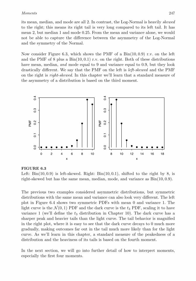
Moments 247
its mean, median, and mode are all 2. In contrast, the Log-Normal is heavily skewedto the right; this means its right tail is very long compared to its left tail. It hasmean 2, but median 1 and mode 0.25. From the mean and variance alone, we wouldnot be able to capture the di↵erence between the asymmetry of the Log-Normaland the symmetry of the Normal.
Now consider Figure 6.3, which shows the PMF of a Bin(10, 0.9) r.v. on the leftand the PMF of 8 plus a Bin(10, 0.1) r.v. on the right. Both of these distributionshave mean, median, and mode equal to 9 and variance equal to 0.9, but they lookdrastically di↵erent. We say that the PMF on the left is left-skewed and the PMFon the right is right-skewed. In this chapter we’ll learn that a standard measure ofthe asymmetry of a distribution is based on the third moment.
0 2 4 6 8 10
0.0
0.1
0.2
0.3
0.4
x
PMF
● ● ● ● ● ●●
●
●
●
●
8 10 12 14 16 18
0.0
0.1
0.2
0.3
0.4
x
PMF
●
●
●
●
●● ● ● ● ● ●
FIGURE 6.3
Left: Bin(10, 0.9) is left-skewed. Right: Bin(10, 0.1), shifted to the right by 8, isright-skewed but has the same mean, median, mode, and variance as Bin(10, 0.9).
The previous two examples considered asymmetric distributions, but symmetricdistributions with the same mean and variance can also look very di↵erent. The leftplot in Figure 6.4 shows two symmetric PDFs with mean 0 and variance 1. Thelight curve is the N (0, 1) PDF and the dark curve is the t
3
PDF, scaling it to havevariance 1 (we’ll define the t
3
distribution in Chapter 10). The dark curve has asharper peak and heavier tails than the light curve. The tail behavior is magnifiedin the right plot, where it is easy to see that the dark curve decays to 0 much moregradually, making outcomes far out in the tail much more likely than for the lightcurve. As we’ll learn in this chapter, a standard measure of the peakedness of adistribution and the heaviness of its tails is based on the fourth moment.
In the next section, we will go into further detail of how to interpret moments,especially the first four moments.

248 Introduction to Probability
−6 −4 −2 0 2 4 6x
0.0
0.2
0.4
0.6
2.5 3.0 3.5 4.0 4.5 5.0
0.000
0.005
0.010
0.015
x
FIGURE 6.4
Left: N (0, 1) PDF (light) and a scaled t3
PDF (dark). Both have mean 0 andvariance 1, but the latter has a sharper peak and heavier tails. Right: magnifiedversion of right tail behavior.
6.2 Interpreting moments
Definition 6.2.1 (Kinds of moments). Let X be an r.v. with mean µ and variance�2. For any positive integer n, the nth moment of X is E(Xn), the nth central mo-
ment is E((X�µ)n), and the nth standardized moment is E(⇣X�µ�
⌘n). Throughout
the previous sentence, “if it exists” is left implicit.
In particular, the mean is the first moment and the variance is the second centralmoment. The term moment is borrowed from physics. Let X be a discrete r.v. withdistinct possible values x
1
, . . . , xn, and imagine a pebble with massmj = P (X = xj)positioned at xj on a number line, for each j (as illustrated in Figure 6.5). Inphysics,
E(X) =nX
j=1
mjxj
is called the center of mass of the system, and
Var(X) =nX
j=1
mj(xj � E(X))2
is called the moment of inertia about the center of mass.
We’ll now define skewness, a single-number summary of asymmetry which, as al-luded to earlier, is based on the third moment. In fact, skewness is defined to bethe third standardized moment.
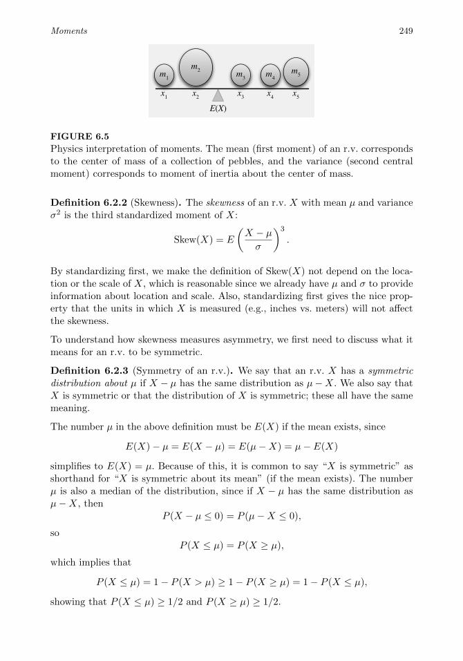
Moments 249
m5
E(X)
m4m1
m2 m3
x1 x2 x3 x4 x5
FIGURE 6.5
Physics interpretation of moments. The mean (first moment) of an r.v. correspondsto the center of mass of a collection of pebbles, and the variance (second centralmoment) corresponds to moment of inertia about the center of mass.
Definition 6.2.2 (Skewness). The skewness of an r.v. X with mean µ and variance�2 is the third standardized moment of X:
Skew(X) = E
✓X � µ
�
◆3
.
By standardizing first, we make the definition of Skew(X) not depend on the loca-tion or the scale of X, which is reasonable since we already have µ and � to provideinformation about location and scale. Also, standardizing first gives the nice prop-erty that the units in which X is measured (e.g., inches vs. meters) will not a↵ectthe skewness.
To understand how skewness measures asymmetry, we first need to discuss what itmeans for an r.v. to be symmetric.
Definition 6.2.3 (Symmetry of an r.v.). We say that an r.v. X has a symmetricdistribution about µ if X � µ has the same distribution as µ�X. We also say thatX is symmetric or that the distribution of X is symmetric; these all have the samemeaning.
The number µ in the above definition must be E(X) if the mean exists, since
E(X)� µ = E(X � µ) = E(µ�X) = µ� E(X)
simplifies to E(X) = µ. Because of this, it is common to say “X is symmetric” asshorthand for “X is symmetric about its mean” (if the mean exists). The numberµ is also a median of the distribution, since if X � µ has the same distribution asµ�X, then
P (X � µ 0) = P (µ�X 0),
soP (X µ) = P (X � µ),
which implies that
P (X µ) = 1� P (X > µ) � 1� P (X � µ) = 1� P (X µ),
showing that P (X µ) � 1/2 and P (X � µ) � 1/2.

250 Introduction to Probability
h 6.2.4. Sometimes people say “X is symmetric” to mean “X is symmetric about0”. Note that ifX is symmetric about µ, thenX�µ is symmetric about 0. Symmetryabout 0 is especially convenient since then �X and X have the same distribution,and the PDF of X (if X is continuous) is an even function, as shown below.
Intuitively, symmetry means that the PDF of X to the left of µ is the mirror imageof the PDF of X to the right of µ (for X continuous, and the same holds for thePMF if X is discrete). For example, we have seen before that X ⇠ N (µ,�2) issymmetric; in terms of the definition, this is because X � µ and µ � X are bothN (0,�2). We have also seen from Corollary 3.3.8 that X ⇠ Bin(n, p) is symmetricwhen p = 1/2.
We can also give an algebraic description of what the PDF of a symmetric continuousr.v. looks like.
Proposition 6.2.5 (Symmetry in terms of the PDF). Let X be a continuousr.v. with PDF f . Then X is symmetric about µ if and only if f(x) = f(2µ� x) forall x.
Proof. Let F be the CDF of X. If symmetry holds, we have
F (x) = P (X � µ x� µ) = P (µ�X x� µ) = P (X � 2µ� x) = 1�F (2µ� x).
Taking the derivative of both sides yields f(x) = f(2µ � x). Conversely, supposethat f(x) = f(2µ� x) holds for all x. Integrating both sides, we have
P (X�µ t) =
Z µ+t
�1f(x)dx =
Z µ+t
�1f(2µ�x)dx =
Z 1
µ�tf(w)dw = P (µ�X t).
⌅
Odd central moments give some information about symmetry.
Proposition 6.2.6 (Odd central moments of a symmetric distribution). Let X besymmetric about its mean µ. Then for any odd number m, the mth central momentE(X � µ)m is 0 if it exists.
Proof. Since X � µ has the same distribution as µ � X, they have the same mthmoment (if it exists):
E(X � µ)m = E(µ�X)m.
Let Y = (X �µ)m. Then (µ�X)m = (�(X �µ))m = (�1)mY = �Y , so the aboveequation just says E(Y ) = �E(Y ). So E(Y ) = 0. ⌅
This leads us to consider using an odd standardized moment as a measure of theskew of a distribution. The first standardized moment is always 0, so the thirdstandardized moment is taken as the definition of skewness. Positive skewness isindicative of having a long right tail relative to the left tail, and negative skewness

Moments 251
is indicative of the reverse. (The converse of the above proposition is false, though:there exist asymmetric distributions whose odd central moments are all 0.)
Why not use, say, the fifth standardized moment instead of the third? One reasonis that the third standardized moment is usually easier to calculate. Another reasonis that we may want to estimate skewness from a data set. It is usually easier toestimate lower moments than higher moments in a stable way since, for example, alarge, noisy observation will have a very large, very noisy fifth power. Nevertheless,just as the mean isn’t the only useful notion of average and the variance isn’t theonly useful notion of spread, the third standardized moment isn’t the only usefulnotion of skew.
Another important descriptive feature of a distribution is how heavy (or long) itstails are. For a given variance, is the variability explained more by a few rare (ex-treme) events or by a moderate number of moderate deviations from the mean?This is an important consideration for risk management in finance: for many fi-nancial assets, the distribution of returns has a heavy left tail caused by rare butsevere crisis events, and failure to account for these rare events can have disastrousconsequences, as demonstrated by the 2008 financial crisis.
As with measuring skew, no single measure can perfectly capture the tail behavior,but there is a widely used summary based on the fourth standardized moment.
Definition 6.2.7 (Kurtosis). The kurtosis of an r.v. X with mean µ and variance�2 is a shifted version of the fourth standardized moment of X:
Kurt(X) = E
✓X � µ
�
◆4
� 3.
h 6.2.8. The reason for subtracting 3 is that this makes any Normal distributionhave kurtosis 0 (as shown in Section 6.5). This provides a convenient basis forcomparison. However, some sources define the kurtosis without the 3, in which casethey call our version “excess kurtosis”.
Roughly speaking, let us call the regions within 1 standard deviation of the mean,between 1 and 2 standard deviations of the mean, and more than 2 standard devi-ations from the mean the center, shoulders, and tails of a distribution, respectively.Then a prototypical distribution with large kurtosis has a PDF with a sharp peakin the center, low shoulders, and heavy tails. For example, the PDF shown in darkin Figure 6.4 fits this description.
Figure 6.6 shows three named distributions and lists the skewness and kurtosis ofeach. The Expo(1) and Pois(4) distributions (left and middle) both have positiveskewness and positive kurtosis, indicating that they are right-skewed and their tailsare heavier than those of a Normal distribution. The Unif(0, 1) distribution (right)has zero skewness and negative kurtosis: zero skewness because the distribution issymmetric about its mean, and negative kurtosis because it has no tails!
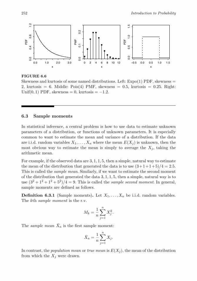
252 Introduction to Probability
0.0 1.0 2.0 3.0
0.0
0.4
0.8
1.2
x
0 2 4 6 8 10 12x
PMF
0.0
0.1
0.2
●
●
●
● ●
●
●
●
●
●● ● ●
−0.5 0.0 0.5 1.0 1.5
0.0
0.5
1.0
1.5
x
FIGURE 6.6
Skewness and kurtosis of some named distributions. Left: Expo(1) PDF, skewness =2, kurtosis = 6. Middle: Pois(4) PMF, skewness = 0.5, kurtosis = 0.25. Right:Unif(0, 1) PDF, skewness = 0, kurtosis = �1.2.
6.3 Sample moments
In statistical inference, a central problem is how to use data to estimate unknownparameters of a distribution, or functions of unknown parameters. It is especiallycommon to want to estimate the mean and variance of a distribution. If the dataare i.i.d. random variables X
1
, . . . , Xn where the mean E(Xj) is unknown, then themost obvious way to estimate the mean is simply to average the Xj , taking thearithmetic mean.
For example, if the observed data are 3, 1, 1, 5, then a simple, natural way to estimatethe mean of the distribution that generated the data is to use (3+1+1+5)/4 = 2.5.This is called the sample mean. Similarly, if we want to estimate the second momentof the distribution that generated the data 3, 1, 1, 5, then a simple, natural way is touse (32 + 12 + 12 + 52)/4 = 9. This is called the sample second moment. In general,sample moments are defined as follows.
Definition 6.3.1 (Sample moments). Let X1
, . . . , Xn be i.i.d. random variables.The kth sample moment is the r.v.
Mk =1
n
nX
j=1
Xkj .
The sample mean Xn is the first sample moment:
Xn =1
n
nX
j=1
Xj .
In contrast, the population mean or true mean is E(Xj), the mean of the distributionfrom which the Xj were drawn.

Moments 253
The law of large numbers, which we prove in Chapter 10, shows that the kth samplemoment of i.i.d. random variables X
1
, . . . , Xn converges to the kth moment E(Xk1
)as n ! 1. Also, the expected value of the kth sample moment is the kth moment.In statistical terms, we say that the kth sample moment is unbiased for estimatingthe kth moment. It is easy to check this by linearity:
E
0
@ 1
n
nX
j=1
Xkj
1
A =1
n
⇣E(Xk
1
) + · · ·+ E(Xkn)⌘= E(Xk
1
).
The mean and variance of the sample mean are often needed, and have nice expres-sions that are often needed in statistics.
Theorem 6.3.2 (Mean and variance of sample mean). Let X1
, . . . , Xn be i.i.d. r.v.swith mean µ and variance �2. Then the sample mean Xn is unbiased for estimatingµ. That is,
E(Xn) = µ.
The variance of Xn is given by
Var(Xn) =�2
n.
Proof. We have E(Xn) = µ since we showed above that the kth sample momentis unbiased for estimating the kth moment. For the variance, we will use the fact(shown in the next chapter) that the variance of the sum of independent r.v.s is thesum of the variances:
Var(Xn) =1
n2
Var(X1
+ · · ·+Xn) =n
n2
Var(X1
) =�2
n.
⌅
For estimating the variance of the distribution of i.i.d. r.v.s X1
, . . . , Xn, a naturalapproach building on the above concepts is to mimic the formula Var(X) = E(X2)�(EX)2 by taking the second sample moment and subtracting the square of thesample mean. There are advantages to this method, but a more common method isas follows.
Definition 6.3.3 (Sample variance and sample standard deviation). LetX
1
, . . . , Xn be i.i.d. random variables. The sample variance is the r.v.
S2
n =1
n� 1
nX
j=1
(Xj � Xn)2.
The sample standard deviation is the square root of the sample variance.

254 Introduction to Probability
The idea of the above definition is to mimic the formula Var(X) = E(X�E(X))2 byaveraging the squared distances of the Xj from the sample mean, except with n� 1rather than n in the denominator. The motivation for the n� 1 is that this makesS2
n unbiased for estimating �2, i.e., it is correct on average. (However, the samplestandard deviation Sn is not unbiased for estimating �; we will see in Chapter10 which way the inequality goes. In any case, unbiasedness is only one of severalcriteria by which to judge an estimation procedure. For example, in some problemswe can get a lower mean squared error in return for allowing a little bit of bias, andthis tradeo↵ may be worthwhile.)
Theorem 6.3.4 (Unbiasedness of sample variance). Let X1
, . . . , Xn be i.i.d. r.v.swith mean µ and variance �2. Then the sample variance S2
n is unbiased for estimating�2, i.e.,
E(S2
n) = �2.
Proof. The key to the proof is the handy identity
nX
j=1
(Xj � c)2 =nX
j=1
(Xj � Xn)2 + n(Xn � c)2,
which holds for all c. To verify the identity, add and subtract Xn in the left-handsum:
nX
j=1
(Xj � c)2 =nX
j=1
�(Xj � Xn) + (Xn � c)
�2
=nX
j=1
(Xj � Xn)2 + 2
nX
j=1
(Xj � Xn)(Xn � c) +nX
j=1
(Xn � c)2
=nX
j=1
(Xj � Xn)2 + n(Xn � c)2.
For the last line, we used the fact that Xn � c does not depend on j and the factthat
nX
j=1
(Xj � Xn) =nX
j=1
Xj �nX
j=1
Xn = nXn � nXn = 0.
Now let us apply the identity, choosing c = µ. Taking the expectation of both sides,
nE(X1
� µ)2 = E
0
@nX
j=1
(Xj � Xn)2
1
A+ nE(Xn � µ)2.
By definition of variance, E(X1
� µ)2 = Var(X1
) = �2, E(Xn � µ)2 = Var(Xn) =�2/n. Plugging these results in above and simplifying, we have E(S2
n) = �2. ⌅
Moments 255
Similarly, we can define the sample skewness to be
1
n
Pnj=1
(Xj � Xn)3
S3
n
,
and the sample kurtosis to be
1
n
Pnj=1
(Xj � Xn)4
S4
n
� 3.
Beyond the fourth moment, it rapidly gets harder to interpret moments graphicallyand harder to estimate them well from data if they are unknown. However, in therest of this chapter we will see that it can still be useful to know all the moments ofa distribution. We will also study a way of computing moments that is often easierthan LOTUS. Both the usefulness and the computation of moments are closelyconnected to a blueprint called the moment generating function, to which we devotemost of the rest of this chapter.
6.4 Moment generating functions
A generating function is a clothesline on which we hang up a sequence ofnumbers for display. – Herbert Wilf [31]
Generating functions are a powerful tool in combinatorics and probability, bridgingbetween sequences of numbers and the world of calculus. In probability, they areuseful for studying both discrete and continuous distributions. The general ideabehind a generating function is as follows: starting with a sequence of numbers,create a continuous function—the generating function—that encodes the sequence.We then have all the tools of calculus at our disposal for manipulating the generatingfunction.
A moment generating function, as its name suggests, is a generating function thatencodes the moments of a distribution. Here is the definition, followed by a fewexamples.
Definition 6.4.1 (Moment generating function). The moment generating function(MGF) of an r.v. X is M(t) = E(etX), as a function of t, if this is finite on someopen interval (�a, a) containing 0. Otherwise we say the MGF of X does not exist.
A natural question at this point is “What is the interpretation of t?” The answeris that t has no interpretation in particular; it’s just a bookkeeping device that weintroduce in order to be able to use calculus instead of working with a discretesequence of moments.
Note that M(0) = 1 for any valid MGF M ; whenever you compute an MGF, plugin 0 and see if you get 1, as a quick check!

256 Introduction to Probability
Example 6.4.2 (Bernoulli MGF). For X ⇠ Bern(p), etX takes on the value et withprobability p and the value 1 with probability q, so M(t) = E(etX) = pet+ q. Sincethis is finite for all values of t, the MGF is defined on the entire real line. ⇤Example 6.4.3 (Geometric MGF). For X ⇠ Geom(p),
M(t) = E(etX) =1X
k=0
etkqkp = p
1X
k=0
(qet)k =p
1� qet
for qet < 1, i.e., for t in (�1, log(1/q)), which is an open interval containing 0. ⇤Example 6.4.4 (Uniform MGF). Let U ⇠ Unif(a, b). Then the MGF of U is
M(t) = E(etU ) =1
b� a
Z b
aetudu =
etb � eta
t(b� a)
for t 6= 0, and M(0) = 1. ⇤The next three theorems give three reasons why the MGF is important. First, theMGF encodes the moments of an r.v. Second, the MGF of an r.v. determines itsdistribution, like the CDF and PMF/PDF. Third, MGFs make it easy to find thedistribution of a sum of independent r.v.s. Let’s take these one by one.
Theorem 6.4.5 (Moments via derivatives of the MGF). Given the MGF of X, wecan get the nth moment of X by evaluating the nth derivative of the MGF at 0:E(Xn) = M (n)(0).
Proof. This can be seen by noting that the Taylor expansion of M(t) about 0 is
M(t) =1X
n=0
M (n)(0)tn
n!,
while on the other hand, we also have
M(t) = E(etX) = E
1X
n=0
Xn tn
n!
!.
We are allowed to interchange the expectation and the infinite sum because certaintechnical conditions are satisfied (this is where we invoke the condition that E(etX)is finite in an interval around 0), so
M(t) =1X
n=0
E(Xn)tn
n!.
Matching the coe�cients of the two expansions, we get E(Xn) = M (n)(0). ⌅
The above theorem is surprising in that for a continuous r.v. X, to compute mo-ments would seemingly require doing integrals with LOTUS, but with the MGF itis possible to find moments by taking derivatives rather than doing integrals!

Moments 257
Theorem 6.4.6 (MGF determines the distribution). The MGF of a random vari-able determines its distribution: if two r.v.s have the same MGF, they must havethe same distribution. In fact, if there is even a tiny interval (�a, a) containing 0on which the MGFs are equal, then the r.v.s must have the same distribution.
The above theorem is a di�cult result in analysis, so we will not prove it here.
Theorem 6.4.7 (MGF of a sum of independent r.v.s). If X and Y are independent,then the MGF of X + Y is the product of the individual MGFs:
MX+Y (t) = MX(t)MY (t).
This is true because if X and Y are independent, then E(et(X+Y )) = E(etX)E(etY )(this follows from results discussed in Chapter 7). Using this fact, we can get theMGFs of the Binomial and Negative Binomial, which are sums of independentBernoullis and Geometrics, respectively.
Example 6.4.8 (Binomial MGF). The MGF of a Bern(p) r.v. is pet + q, so theMGF of a Bin(n, p) r.v. is
M(t) = (pet + q)n.
−1.0 −0.5 0.0 0.5 1.0
01
23
4
t
MGF
FIGURE 6.7
Bin(2, 1/2) MGF, M(t) =�1
2
et + 1
2
�2
. The slope of the MGF at t = 0 is 1, so themean of the distribution is 1. The concavity or second derivative of the MGF att = 0 is 3/2, so the second moment of the distribution is 3/2.
Figure 6.7 plots the MGF of the Bin(2, 1/2) distribution, M(t) =�1
2
et + 1
2
�2
, be-tween t = �1 and t = 1. As with all MGFs, the value of the MGF is 1 at t = 0.Furthermore, the first and second moments of the distribution are the first andsecond derivatives of the MGF, evaluated at t = 0; these correspond to the slopeand concavity of the plotted curve at t = 0. These two derivatives are 1 and 3/2

258 Introduction to Probability
respectively, corresponding to the fact that the Bin(2, 1/2) distribution has mean 1and variance 3/2� 12 = 1/2. ⇤Example 6.4.9 (Negative Binomial MGF). We know the MGF of a Geom(p) r.v. is
p1�qet for qet < 1, so the MGF of X ⇠ NBin(r, p) is
M(t) =
✓p
1� qet
◆r
for qet < 1. ⇤h 6.4.10. Not all r.v.s have an MGF. Some r.v.s X don’t even have E(X) exist,or don’t have E(Xn) exist for some n > 1, in which case the MGF clearly will notexist. But even if all the moments of X exist, the MGF may not exist if the momentsgrow too quickly. Luckily, there is a way to fix this: inserting an imaginary number!The function (t) = E(eitX) with i =
p�1 is called the characteristic function
by statisticians and the Fourier transform by everyone else. It turns out that thecharacteristic function always exists. In this book we will focus on the MGF ratherthan the characteristic function, to avoid having to handle imaginary numbers.
As we saw in the previous chapter, location and scale transformations are a fun-damental way to build a family of distributions from an initial distribution. Forexample, starting with Z ⇠ N (0, 1), we can scale by � and shift by µ to obtainX = µ + �Z ⇠ N (µ,�2). In general, if we have an r.v. X with mean µ and stan-dard deviation � > 0, we can create the standardized version (X � µ)/�, and viceversa. Conveniently, it is easy to relate the MGFs of two r.v.s connected by such atransformation.
Proposition 6.4.11 (MGF of location-scale transformation). If X has MGF M(t),then the MGF of a+ bX is
E(et(a+bX)) = eatE(ebtX) = eatM(bt).
For example, let’s use this proposition to help obtain the MGFs of the Normal andExponential distributions.
Example 6.4.12 (Normal MGF). The MGF of a standard Normal r.v. Z is
MZ(t) = E(etZ) =
Z 1
�1etz
1p2⇡
e�z2/2dz.
After completing the square, we have
MZ(t) = et2/2
Z 1
�1
1p2⇡
e�(z�t)2/2dz = et2/2,
using the fact that theN (t, 1) PDF integrates to 1. Thus, the MGF ofX = µ+�Z ⇠N (µ,�2) is
MX(t) = eµtMZ(�t) = eµte(�t)2/2 = eµt+
1
2
�2t2 .
⇤
Moments 259
Example 6.4.13 (Exponential MGF). The MGF of X ⇠ Expo(1) is
M(t) = E(etX) =
Z 1
0
etxe�xdx =
Z 1
0
e�x(1�t)dx =1
1� tfor t < 1.
So the MGF of Y = X/� ⇠ Expo(�) is
MY (t) = MX
✓t
�
◆=
�
�� tfor t < �.
⇤
6.5 Generating moments with MGFs
We now give some examples of where the MGF got its name from. Theorem 6.4.5shows that we can get moments by di↵erentiating the MGF and evaluating at 0,rather than doing a complicated sum or integral by LOTUS. Better yet, in somecases we can simultaneously find all the moments of a distribution via a Taylorexpansion, rather than di↵erentiating over and over again.
Example 6.5.1 (Exponential moments). In this example we will show how touse the Exponential MGF to get all the moments of the Exponential distributionsimultaneously! Let X ⇠ Expo(1). The MGF of X is M(t) = 1/(1� t) for t < 1.
As shown in Theorem 6.4.5, we could obtain the moments by taking derivativesof the MGF and evaluating at 0. In this case, though, we recognize 1/(1 � t) as ageometric series, valid in an interval around 0. For |t| < 1,
M(t) =1
1� t=
1X
n=0
tn =1X
n=0
n!tn
n!.
On the other hand, we know that E(Xn) is the coe�cient of the term involving tn
in the Taylor expansion of M(t):
M(t) =1X
n=0
E(Xn)tn
n!.
Thus we can match coe�cients to conclude that E(Xn) = n! for all n. We not onlydid not have to do a LOTUS integral, but also we did not, for example, have totake 10 derivatives to get the 10th moment—we got the moments all at once.
To find the moments of Y ⇠ Expo(�), use a scale transformation: we can expressY = X/� where X ⇠ Expo(1). Therefore Y n = Xn/�n and
E(Y n) =n!
�n.

260 Introduction to Probability
In particular, we have found the mean and variance of Y , making good on ourpromise from Chapter 5:
E(Y ) =1
�,
Var(Y ) = E(Y 2)� (EY )2 =2
�2� 1
�2=
1
�2.
⇤Example 6.5.2 (Standard Normal moments). In this example we will find all themoments of the standard Normal distribution. Let Z ⇠ N (0, 1). We can use thesame trick of matching the coe�cients of the Taylor expansion.
M(t) = et2/2 =
1X
n=0
(t2/2)n
n!=
1X
n=0
t2n
2nn!=
1X
n=0
(2n)!
2nn!
t2n
(2n)!.
Therefore
E(Z2n) =(2n)!
2nn!,
and the odd moments of Z are equal to 0, which must be true due to the symmetryof the standard Normal. From the story proof about partnerships in Example 1.5.4,we know that (2n)!
2
nn! is also equal to the skip factorial (2n� 1)!!, so we have E(Z2) =1, E(Z4) = 1 · 3, E(Z6) = 1 · 3 · 5, etc.
This result also shows that the kurtosis of the Normal distribution is 0. Let X ⇠N (µ,�2); then
Kurt(X) = E
✓X � µ
�
◆4
� 3 = E(Z4)� 3 = 3� 3 = 0.
⇤Example 6.5.3 (Log-Normal moments). Now let’s consider the Log-Normal dis-tribution. We say that Y is Log-Normal with parameters µ and �2, denoted byY ⇠ LN (µ,�2), if Y = eX where X ⇠ N (µ,�2).
h 6.5.4. Log-Normal does not mean “log of a Normal”, since a Normal can benegative. Rather, Log-Normal means “log is Normal”. It is important to distinguishbetween the mean and variance of the Log-Normal and the mean and variance ofthe underlying Normal. Here we are defining µ and �2 to be the mean and varianceof the underlying Normal, which is the most common convention.
Interestingly, the Log-Normal MGF does not exist, since E(etY ) is infinite for allt > 0. Consider the case where Y = eZ for Z ⇠ N (0, 1); by LOTUS,
E(etY ) = E(eteZ
) =
Z 1
�1ete
z 1p2⇡
e�z2/2dz =
Z 1
�1
1p2⇡
etez�z2/2dz.
For any t > 0, tez � z2/2 goes to infinity as z grows, so the above integral diverges.

Moments 261
Since E(etY ) is not finite on an open interval around 0, the MGF of Y does notexist. The same reasoning holds for a general Log-Normal distribution.
However, even though the Log-Normal MGF does not exist, we can still obtain allthe moments of the Log-Normal, using the MGF of the Normal. For Y = eX withX ⇠ N (µ,�2),
E(Y n) = E(enX) = MX(n) = enµ+1
2
n2�2
.
In other words, the nth moment of the Log-Normal is the MGF of the Normalevaluated at t = n. Letting
m = E(Y ) = eµ+1
2
�2
,
we have after some algebra
Var(Y ) = E(Y 2)�m2 = m2(e�2 � 1).
All Log-Normal distributions are right-skewed. For example, Figure 6.2 shows aLog-Normal PDF in dark, with mean 2 and variance 12. This is the distributionof eX for X ⇠ N (0, 2 log 2), and it is clearly right-skewed. To quantify this, let uscompute the skewness of the Log-Normal r.v. Y = eX for X ⇠ N (0,�2). Lettingm = E(Y ) = e
1
2
�2
, we have E(Y n) = mn2
and Var(Y ) = m2(m2� 1), and the thirdcentral moment is
E(Y �m)3 = E(Y 3 � 3mY 2 + 3m2Y �m3)
= E(Y 3)� 3mE(Y 2) + 2m3
= m9 � 3m5 + 2m3.
Thus, the skewness is
Skew(Y ) =E(Y �m)3
SD3(Y )=
m9 � 3m5 + 2m3
m3(m2 � 1)3/2= (m2 + 2)
pm2 � 1,
where in the last step we factored m6 � 3m2 + 2 = (m2 + 2)(m� 1)2(m+ 1)2. Theskewness is positive since m > 1, and it increases very quickly as � grows. ⇤
6.6 Sums of independent r.v.s via MGFs
Since the MGF of a sum of independent r.v.s is just the product of the individ-ual MGFs, we now have a new strategy for finding the distribution of a sum ofindependent r.v.s: multiply the individual MGFs together and see if the productis recognizable as the MGF of a named distribution. The next two examples illus-trate.

262 Introduction to Probability
Example 6.6.1 (Sum of independent Poissons). Using MGFs, we can easily showthat the sum of independent Poissons is Poisson. First let’s find the MGF of X ⇠Pois(�):
E(etX) =1X
k=0
etke���k
k!= e��
1X
k=0
(�et)k
k!= e��e�e
t
= e�(et�1).
Now let Y ⇠ Pois(µ) be independent of X. The MGF of X + Y is
E(etX)E(etY ) = e�(et�1)eµ(e
t�1) = e(�+µ)(et�1),
which is the Pois(�+µ) MGF. Since the MGF determines the distribution, we haveproven that X + Y ⇠ Pois(� + µ). Contrast this with the proof from Chapter 4(Theorem 4.8.1), which required using the law of total probability and summingover all possible values of X. The proof using MGFs is far less tedious. ⇤h 6.6.2. It is important that X and Y be independent in the above example. To seewhy, consider an extreme form of dependence: X = Y . In that case, X + Y = 2X,which can’t possibly be Poisson since its value is always an even number!
Example 6.6.3 (Sum of independent Normals). If we have X1
⇠ N (µ1
,�21
) andX
2
⇠ N (µ2
,�22
) independently, then the MGF of X1
+X2
is
MX1
+X2
(t) = MX1
(t)MX2
(t) = eµ1
t+ 1
2
�2
1
t2 · eµ2
t+ 1
2
�2
2
t2 = e(µ1
+µ2
)t+ 1
2
(�2
1
+�2
2
)t2 ,
which is the N (µ1
+ µ2
,�21
+ �22
) MGF. Again, because the MGF determines thedistribution, it must be the case that X
1
+X2
⇠ N (µ1
+µ2
,�21
+�22
). Thus the sumof independent Normals is Normal, and the means and variances simply add. ⇤Example 6.6.4 (Sum is Normal). A converse to the previous example also holds: ifX
1
andX2
are independent andX1
+X2
is Normal, thenX1
andX2
must be Normal!This is known as Cramer’s theorem. Proving this in full generality is di�cult, butit becomes much easier if X
1
and X2
are i.i.d. with MGF M(t). Without loss ofgenerality, we can assume X
1
+X2
⇠ N (0, 1), and then its MGF is
et2/2 = E(et(X1
+X2
)) = E(etX1)E(etX2) = (M(t))2,
so M(t) = et2/4, which is the N (0, 1/2) MGF. Thus, X
1
, X2
⇠ N (0, 1/2). ⇤In Chapter 8 we’ll discuss a more general technique for finding the distribution ofa sum of r.v.s when the individual MGFs don’t exist, or when the product of theindividual MGFs is not recognizable and we would like to obtain the PMF/PDFinstead.
6.7 *Probability generating functions
In this section we discuss probability generating functions, which are similar to MGFsbut are guaranteed to exist for nonnegative integer-valued r.v.s. First we’ll use PGFs

Moments 263
to conquer a seemingly intractable counting problem. Then we’ll prove that the PGFof a nonnegative integer-valued r.v. determines its distribution, which we omittedin the more general MGF setting.
Definition 6.7.1 (Probability generating function). The probability generatingfunction (PGF) of a nonnegative integer-valued r.v. X with PMF pk = P (X = k)is the generating function of the PMF. By LOTUS, this is
E(tX) =1X
k=0
pktk.
The PGF converges to a value in [�1, 1] for all t in [�1, 1] sinceP1
k=0
pk = 1 and|pktk| pk for |t| 1.
The MGF is closely related to the PGF, when both exist: for t > 0,
E(tX) = E(eX log t)
is the MGF evaluated at log t.
Example 6.7.2 (Generating dice probabilities). Frederick Mosteller, the founderof the Harvard Statistics Department, once recounted the following life-changingmoment:
A key moment in my life occurred in one of those classes during my sophomoreyear. We had the question: When three dice are rolled what is the chance thatthe sum of the faces will be 10? The students in this course were very good, butwe all got the answer largely by counting on our fingers. When we came to class,I said to the teacher, “That’s all very well—we got the answer—but if we hadbeen asked about six dice and the probability of getting 18, we would still behome counting. How do you do problems like that?” He said, “I don’t know, butI know a man who probably does and I’ll ask him.”
One day I was in the library and Professor Edwin G. Olds of the MathematicsDepartment came in. He shouted at me, “I hear you’re interested in the threedice problem.” He had a huge voice, and you know how libraries are. I wasembarrassed. “Well, come and see me,” he said, “and I’ll show you about it.”“Sure,” I said. But I was saying to myself, “I’ll never go.” Then he said, “Whatare you doing?” I showed him. “That’s nothing important,” he said. “Let’s gonow.”
So we went to his o�ce, and he showed me a generating function. It wasthe most marvelous thing I had ever seen in mathematics. It used mathematicsthat, up to that time, in my heart of hearts, I had thought was something thatmathematicians just did to create homework problems for innocent students inhigh school and college. I don’t know where I had got ideas like that aboutvarious parts of mathematics. Anyway, I was stunned when I saw how Olds usedthis mathematics that I hadn’t believed in. He used it in such an unusuallyoutrageous way. It was a total retranslation of the meaning of the numbers. [1]
264 Introduction to Probability
Let X be the total from rolling 6 fair dice, and let X1
, . . . , X6
be the individualrolls. What is P (X = 18)? It turns out that there are 3431 ways to obtain a sum of18, so the probability is 3431/66 ⇡ 0.0735. Listing out all possibilities is extremelytedious, and the tedium would be compounded with the worry of having somehowmissed a case. And what if we laboriously listed out all 3431 cases, and then wereasked to find P (X = 19)?
The PGF of X will allow us to count the cases in a systematic way. The PGF ofX
1
is
E(tX1) =1
6(t+ t2 + · · ·+ t6).
Since the Xj are i.i.d., the PGF of X is
E�tX�= E
�tX1 · · · tX6
�= E
�tX1
�· · ·E
�tX6
�=
t6
66(1 + t+ · · ·+ t5)6.
By definition, the coe�cient of t18 in the PGF is P (X = 18). So the number ofways to get a sum of 18 is the coe�cient of t18 in t6(1 + t+ · · ·+ t5)6, which is thecoe�cient of t12 in (1 + t+ · · ·+ t5)6. Multiplying this out by hand is tedious, butit is vastly easier than listing out 3431 cases, and it can also be done easily on acomputer without having to write a special program.
Better yet, we can use the fact that 1 + t+ · · ·+ t5 is a geometric series to write
(1 + t+ · · ·+ t5)6 =(1� t6)6
(1� t)6.
(Assume that |t| < 1, which we can do since, as with the MGF, we just need toknow how the PGF behaves in an open interval containing 0.) The above equationis just algebra since we have the bookkeeping device t, but would have been hardto fathom if everything were still in sequence notation. By the binomial theorem,the numerator is
(1� t6)6 =6X
j=0
✓6
j
◆(�1)jt6j .
For the denominator, write
1
(1� t)6= (1 + t+ t2 + · · · )6 =
1X
k=0
aktk.
Here ak is the number of ways to choose one term from each of the six (1+t+t2+. . . )factors, such that the degrees add up to k. For example, for k = 20 one possibilityis to choose the t3, 1, t2, t10, 1, t5 terms, respectively, since these choices contributeone t20 term when the product is expanded out. So ak is the number of solutions toy1
+ y2
+ · · ·+ y6
= k, with the yj nonnegative integers. We saw how to count this
number of solutions in Chapter 1: ak is the Bose-Einstein value�6+k�1
k
�=�k+5
5
�. So
1
(1� t)6=
1X
k=0
✓k + 5
5
◆tk.

Moments 265
For 0 < t < 1, another way to see why this equation holds is to write it as
1X
k=0
✓k + 5
5
◆(1� t)6tk = 1,
which we already knew to be true since the NBin(6, 1�t) PMF must sum to 1. (Theidentity for (1 � t)�6 is an example of a generalization of the binomial theorem toallow for negative integer powers; this helps explain where the Negative Binomialgets its name from, considering that a Negative Binomial is neither negative norBinomial!)
Putting together the above results, we just need the coe�cient of t12 in0
@2X
j=0
✓6
j
◆(�1)jt6j
1
A
12X
k=0
✓k + 5
5
◆tk
!,
where we summed only up to j = 2 and k = 12 in the two factors since any furtherterms will not contribute to the coe�cient of t12. This lets us reduce the 3431 casesdown to just three cases: (j, k) is (0, 12), (1, 6), or (2, 0). The coe�cient of t12 is
✓17
5
◆� 6
✓11
5
◆+
✓6
2
◆= 3431,
since, for example, when j = 1 and k = 6 we get the term
�✓6
1
◆t6 ·✓6 + 5
5
◆t6 = �6
✓11
5
◆t12.
Thus,
P (X = 18) =3431
66.
⇤Since the PGF is just a handy bookkeeping device for the PMF, it fully determinesthe distribution (for any nonnegative integer-valued r.v.). The theorem below showshow to pluck the PMF values down from the “clothesline” of the PGF.
Theorem 6.7.3. Let X and Y be nonnegative integer-valued r.v.s, with PGFsgX and gY respectively. Suppose that gX(t) = gY (t) for all t in (�a, a), where0 < a < 1. Then X and Y have the same distribution, and their PMF can berecovered by taking derivatives of gX :
P (X = k) = P (Y = k) =g(k)X (0)
k!.
Proof. Write
gX(t) =1X
k=0
pktk.

266 Introduction to Probability
Then gX(0) = p0
, so P (X = 0) has been recovered—from knowing the function gX ,we can extract the value of P (X = 0). The derivative is
g0X(t) =1X
k=1
kpktk�1,
so g0X(0) = p1
(swapping the derivative and the infinite sum is justified by resultsin real analysis). Then P (X = 1) has been recovered. Continuing in this way, wecan recover the entire PMF by taking derivatives. ⌅Example 6.7.4. Let X ⇠ Bin(n, p). The PGF of a Bern(p) r.v. is pt + q (withq = 1� p), so the PGF of X is g(t) = (pt+ q)n. The above theorem says that anyr.v. with this PGF must in fact be Binomial. Furthermore, we can recover the PMFby computing
g(0) = qn, g0(0) = npqn�1, g00(0)/2! =
✓n
2
◆p2qn�2,
and so on. We can avoid having to take derivatives by using the binomial theoremto write
g(t) = (pt+ q)n =nX
k=0
✓n
k
◆pkqn�ktk,
from which we can directly read o↵ the Binomial PMF.
While we’re working with the Binomial PGF, let’s see how it can be used to get themoments of a Binomial. Letting pk = P (X = k), we have
g0(t) = np(pt+ q)n�1 =nX
k=1
kpktk�1,
so
g0(1) = np =nX
k=1
kpk = E(X).
Taking the derivative again,
g00(t) = n(n� 1)p2(pt+ q)n�2 =nX
k=2
k(k � 1)pktk�2,
soE(X(X � 1)) = g00(1) = n(n� 1)p2.
Rearranging these results gives another proof that Var(X) = npq. Continuing inthis way, we have computed what are called the factorial moments of the Binomial:
E(X(X � 1) . . . (X � k + 1)) = k!
✓n
k
◆pk.
Dividing by k! on both sides, this implies E�Xk
�=�nk
�pk, which can also be seen

Moments 267
with a story proof:�Xk
�is the number of ways to choose k out of the X successful
Bernoulli trials, which is the number of ways to choose k out of the n original trialssuch that all k are successes. Creating an indicator r.v. for each of the
�nk
�subsets
of size k and using linearity, the result follows. ⇤
6.8 Recap
A useful way to study a distribution is via its moments. The first 4 moments arewidely used as a basis for quantitatively describing what the distribution looks like,though many other descriptions are also possible. In particular, the first momentis the mean, the second central moment is the variance, the third standardizedmoment measures skew (asymmetry), and the fourth standardized moment minus 3measures how sharp the peak is and how heavy the tails are, roughly speaking.
Moments are useful for far more than studying the location and shape of a dis-tribution, especially when the moment generating function (MGF) exists (which isstronger than saying that all the moments exist). MGFs are useful for three mainreasons: for computing moments (as an alternative to LOTUS), for studying sumsof independent r.v.s, and since they fully determine the distribution and thus serveas an additional blueprint for a distribution.
Figure 6.8 augments our map of the connections between fundamental objects inprobability. If the MGF of X exists, the sequence E(X), E(X2), E(X3), . . . of mo-ments provides enough information (at least in principle) to determine the distri-bution of X.
6.9 R
Functions
The MGF of an r.v. is a function. As an example of defining and working withfunctions in R, let’s use the N (0, 1) MGF, which is given by M(t) = et
2/2. Thecode
M <- function(t) {exp(t^2/2)}
defines M to be this function. The function(t) says that we’re defining a functionof one variable t (called the argument of the function). Then, for example, M(0)evaluates the function at 0, M(1:10) evaluates the function at 1, 2, . . . , 10, andcurve(M,from=-3,to=3) plots the graph of M from �3 to 3. Writing

268 Introduction to Probability
CDF FPMF (discrete)
PDF (continuous)story
name, parametersMGF
XP(X ≤ x) = F(x)
P(X = x)
func
tion o
f r.v.
X ≤ xX = x
generate
E(X), Var(X), SD(X)
X, X2, X3, …g(X)
LOTUS E(X), E(X2), E(X3), …E(g(X))
distributions random variables numbersevents
What can happen?
P
-6 -4 -2 0 2 4 6
0.00.2
0.40.6
0.81.0
x
F(x)
find the MGF
FIGURE 6.8
For an r.v. X, we can study its moments E(X), E(X2), . . . . These can be computedusing LOTUS or by the MGF (if it exists). If the MGF exists, it determines thedistribution, taking us full circle and adding to our list of blueprints.
M <- function(x) {exp(x^2/2)}
would define the same function M , except that now the argument is named x.Giving the arguments names is helpful for functions of more than one variable,since R then saves us from having to remember the order in which to write thearguments, and allows us to assign default values. For example, the N (µ,�2) MGFis given by g(t) = exp(µt + �2t2/2), which depends on t, µ, and �. We can definethis in R by
g <- function(t,mean=0,sd=1) {exp(mean*t + sd^2*t^2/2)}
What is g(1,2,3)? It’s the N (2, 32) MGF evaluated at 1, but it may be hardto remember which argument is which, especially when working with many func-tions with many arguments over the course of many months. So we can also writeg(t=1,mean=2,sd=3) or g(mean=2,sd=3,t=1) or any of the other 4 permutationsto mean the same thing.
Also, when defining g we specified default values of 0 for the mean and 1 forthe standard deviation, so if we want the N (0, 52) MGF evaluated at 3, wecan use g(t=3,sd=5) as shorthand. It would be bad here to write g(3,5), sincethat is ambiguous about which argument is omitted; in fact, R interprets this asg(t=3,mean=5).

Moments 269
Moments
LOTUS makes it easy to write down any moment of a continuous r.v. as an integral,and then R can help us do the integral numerically, using the integrate command.For example, let’s approximate the 6th moment of a N (0, 1) r.v. The code
g <- function(x) x^6*dnorm(x)
integrate(g, lower = -Inf, upper = Inf)
asks R to computeR1�1 g(x)dx, where g(x) = x6'(x) with ' theN (0, 1) PDF. When
we ran this, R reported 15 (the correct answer, as we know from this chapter!) andthat the absolute error was less than 7.9 ⇥ 10�5. Similarly, to check that the 2ndmoment (and variance) of a Unif(�1, 1) r.v. is 1/3, we can use
h <- function(x) x^2*dunif(x,-1,1)
integrate(h, lower = -1, upper = 1)
h 6.9.1. Numerical integration runs into di�culties for some functions; as usual,checking answers in multiple ways is a good idea. Using upper = Inf is preferred tousing a large number as the upper limit when integrating up to 1 (and likewise fora lower limit of �1). For example, on many systems integrate(dnorm,0,10^6)reports 0 while integrate(dnorm,0,Inf) reports the correct answer, 0.5.
For moments of a discrete r.v., we can use LOTUS and the sum command. Forexample, to find the 2nd moment of X ⇠ Pois(7), we can use
g <- function(k) k^2*dpois(k,7)
sum(g(0:100))
Here we summed up to 100 since it’s clear after getting a sense of the terms thatthe total contribution of all the terms after k = 100 is negligible (choosing anupper limit in this way is in contrast to how to use the integrate command inthe continuous case). The result is extremely close to 56, which is comforting sinceE(X2) = Var(X) + (EX)2 = 7 + 49 = 56.
A sample moment can be found in one line in R. If x is a vector of data, then mean(x)
gives its sample mean and, more generally, mean(x^n) gives the nth sample meanfor any positive integer n. For example,
x <- rnorm(100)
mean(x^6)
gives the 6th sample moment of 100 i.i.d. N (0, 1) r.v.s. How close is it to thetrue 6th moment? How close are other sample moments to the corresponding truemoments?
The sample variance can also be found in one line in R. If x is a vector of data, thenvar(x) gives its sample variance. This returns NA (not available) if x has length 1,since the n� 1 in the denominator is 0 in this case. It makes sense not to return anumerical value in this case, not only because of the definition but also because it
270 Introduction to Probability
would be insane to try to estimate the variability of a population if we only haveone observation!
For a simple demonstration of using the sample mean and sample variance to es-timate the true mean and true variance of a distribution, we generate 1000 timesfrom a N (0, 1) distribution and store the values in z. We then compute the samplemean and sample variance with mean and var.
z <- rnorm(1000)
mean(z)
var(z)
We find that mean(z) is close to 0 and var(z) is close to 1. You can try this outfor a N (µ,�2) distribution (or other distribution) of your choosing; just rememberthat rnorm takes � and not �2 as an input!
The sample standard deviation of x can be found using sd(x). This gives the sameresult as sqrt(var(x)).
R does not come with built-in functions for sample skewness or sample kurtosis,but we can define our own functions as follows.
skew <- function(x) {
centralmoment <- mean((x-mean(x))^3)
centralmoment/(sd(x)^3)
}
kurt <- function(x) {
centralmoment <- mean((x-mean(x))^4)
centralmoment/(sd(x)^4) - 3
}
Medians and modes
To find the median of a continuous r.v. with CDF F , we need to solve the equationF (x) = 1/2 for x, which is equivalent to finding the root (zero) of the function ggiven by g(x) = F (x) � 1/2. This can be done using uniroot in R. For example,let’s find the median of the Expo(1) distribution. The code
g <- function(x) pexp(x) - 1/2
uniroot(g,lower=0,upper=1)
asks R to find a root of the desired function between 0 and 1. This returns an answervery close to the true answer of log(2) ⇡ 0.693. Of course, in this case we can solve1� e�x = 1/2 directly without having to use numerical methods.
h 6.9.2. The uniroot command is useful but it only attempts to find one root (asthe name suggests), and there is no guarantee that it will find a root.
Moments 271
An easier way to find the median of the Expo(1) in R is to use qexp(1/2). Thefunction qexp is the quantile function of the Expo(1) distribution, which means thatqexp(p) is the value of x such that P (X x) = p for X ⇠ Expo(1).
For finding the mode of a continuous distribution, we can use the optimize functionin R. For example, let’s find the mode of the Gamma(6, 1) distribution, which isan important distribution that we will introduce in the next chapter. Its PDF isproportional to x5e�x. Using calculus, we can find that the mode is at x = 5. UsingR, we can find that the mode is very close to x = 5 as follows.
h <- function(x) x^5*exp(-x)
optimize(h,lower=0,upper=20,maximum=TRUE)
If we had wanted to minimize instead of maximize, we could have putmaximum=FALSE.
Next, let’s do a discrete example of median and mode. An interesting fact aboutthe Bin(n, p) distribution is that if the mean np is an integer, then the median andmode are also np (even if the distribution is very skewed). To check this fact aboutthe median for the Bin(50, 0.2) distribution, we can use the following code.
n <- 50; p <- 0.2
which.max(pbinom(0:n,n,p)>=0.5)
The which.max function finds the location of the maximum of a vector, giving theindex of the first occurrence of a maximum. Since TRUE is encoded as 1 and FALSEis encoded as 0, the first maximum in pbinom(0:n,n,p)>=0.5 is at the first valuefor which the CDF is at least 0.5. The output of the above code is 11, but we must becareful to avoid an o↵-by-one error: the index 11 corresponds to the median being 10,since we started evaluating the CDF at 0. Similarly, which.max(dbinom(0:n,n,p))returns 11, showing that the mode is at 10.
The sample median of a vector x of data can be found using median(x). Butmode(x) does not give the sample mode of x (rather, it gives information aboutwhat type of object x is). To find the sample mode (or sample modes, in case thereare ties), we can use the following function.
datamode <- function(x) {
t <- table(x)
m <- max(t)
as.numeric(names(t[t==m]))
}
Dice simulation
In the starred Section 6.7, we showed that in rolling 6 fair dice, the probabilityof a total of 18 is 3431/66. But the proof was complicated. If we only need an

272 Introduction to Probability
approximate answer, simulation is a much easier approach. And we already knowhow to do it! Here is the code for a million repetitions:
r <- replicate(10^6,sum(sample(6,6,replace=TRUE)))
sum(r==18)/10^6
In our simulation this yielded 0.07346, which is very close to 3431/66 ⇡0.07354.
6.10 Exercises
Means, medians, modes, and moments
1. Let U ⇠ Unif(a, b). Find the median and mode of U .
2. Let X ⇠ Expo(�). Find the median and mode of X.
3. Let X have the Pareto distribution with parameter a > 0; this means that X has PDFf(x) = a/xa+1 for x � 1 (and 0 otherwise). Find the median and mode of X.
4. Let X ⇠ Bin(n, p).
(a) For n = 5, p = 1/3, find all medians and all modes of X. How do they compare tothe mean?
(b) For n = 6, p = 1/3, find all medians and all modes of X. How do they compare tothe mean?
5. Let X be Discrete Uniform on 1, 2, . . . , n. Find all medians and all modes of X (youranswer can depend on whether n is even or odd).
6. Suppose that we have data giving the amount of rainfall in a city each day in a certainyear. We want useful, informative summaries of how rainy the city was that year. Onthe majority of days in that year, it did not rain at all in the city. Discuss and comparethe following six summaries: the mean, median, and mode of the rainfall on a randomlychosen day from that year, and the mean, median, and mode of the rainfall on a randomlychosen rainy day from that year (where by “rainy day” we mean that it did rain thatday in the city).
7. Let a and b be positive constants. The Beta distribution with parameters a and b,which we introduce in detail in Chapter 8, has PDF proportional to xa�1(1� x)b�1 for0 < x < 1 (and the PDF is 0 outside of this range). Show that for a > 1, b > 1, themode of the distribution is (a� 1)/(a+ b� 2).
Hint: Take the log of the PDF first (note that this does not a↵ect where the maximumis achieved).
8. Find the median of the Beta distribution with parameters a = 3 and b = 1 (see theprevious problem for information about the Beta distribution).
9. Let Y be Log-Normal with parameters µ and �2. So Y = eX with X ⇠ N (µ,�2).Evaluate and explain whether or not each of the following arguments is correct.
(a) Student A: “The median of Y is eµ because the median of X is µ and the exponentialfunction is continuous and strictly increasing, so the event Y eµ is the same as theevent X µ.”
(b) Student B: “The mode of Y is eµ because the mode of X is µ, which correspondsto eµ for Y since Y = eX .”

Moments 273
(c) Student C: “The mode of Y is µ because the mode of X is µ and the exponentialfunction is continuous and strictly increasing, so maximizing the PDF of X is equivalentto maximizing the PDF of Y = eX .”
10. A distribution is called symmetric unimodal if it is symmetric (about some point) andhas a unique mode. For example, any Normal distribution is symmetric unimodal. LetX have a continuous symmetric unimodal distribution for which the mean exists. Showthat the mean, median, and mode of X are all equal.
11. Let X1
, . . . , Xn be i.i.d. r.v.s with mean µ, variance �2, and skewness �.
(a) Standardize the Xj by letting
Zj =(Xj � µ)
�.
Let Xn and Zn be the sample means of the Xj and Zj , respectively. Show that Zj hasthe same skewness as Xj , and Zn has the same skewness as Xn.
(b) Show that the skewness of the sample mean Xn is �/pn.
Hint: By (a), we can assume µ = 0 and �2 = 1 without loss of generality; if the Xj arenot standardized initially, then we can standardize them. If (X
1
+ X2
+ · · · + Xn)3 is
expanded out, there are 3 types of terms: terms such as X3
1
, terms such as 3X2
1
X2
, andterms such as 6X
1
X2
X3
.
(c) What does the result of (b) say about the distribution of Xn when n is large?
12. Let c be the speed of light in a vacuum. Suppose that c is unknown, and scientists wishto estimate it. But even more so than that, they wish to estimate c2, for use in thefamous equation E = mc2.
Through careful experiments, the scientists obtain n i.i.d. measurementsX1
, X2
, . . . , Xn ⇠N (c,�2). Using these data, there are various possible ways to estimate c2. Two naturalways are: (1) estimate c using the average of the Xj ’s and then square the estimated c,and (2) average the X2
j ’s. So let
Xn =1n
nX
j=1
Xj ,
and consider the two estimators
T1
= X2
n and T2
=1n
nX
j=1
X2
j .
Note that T1
is the square of the first sample moment and T2
is the second samplemoment.
(a) Find P (T1
< T2
).
Hint: Start by comparing ( 1
n
Pnj=1
xj)2 and 1
n
Pnj=1
x2
j when x1
, . . . , xn are numbers,by considering a discrete r.v. whose possible values are x
1
, . . . , xn.
(b) When an r.v. T is used to estimate an unknown parameter ✓, the bias of the estimatorT is defined to be E(T )� ✓. Find the bias of T
1
and the bias of T2
.
Hint: First find the distribution of Xn. In general, for finding E(Y 2) for an r.v. Y , it isoften useful to write it as E(Y 2) = Var(Y ) + (EY )2.

274 Introduction to Probability
Moment generating functions
13. s� A fair die is rolled twice, with outcomes X for the first roll and Y for the secondroll. Find the moment generating function MX+Y (t) of X + Y (your answer should bea function of t and can contain unsimplified finite sums).
14. s� Let U1
, U2
, . . . , U60
be i.i.d. Unif(0, 1) and X = U1
+ U2
+ · · ·+ U60
. Find the MGFof X.
15. Let W = X2+Y 2, with X,Y i.i.d. N (0, 1). The MGF of X2 turns out to be (1�2t)�1/2
for t < 1/2 (you can assume this).
(a) Find the MGF of W .
(b) What famous distribution that we have studied so far does W follow (be sure tostate the parameters in addition to the name)? In fact, the distribution of W is also aspecial case of two more famous distributions that we will study in later chapters!
16. Let X ⇠ Expo(�). Find the skewness of X, and explain why it is positive and why itdoes not depend on �.
Hint: One way to find the third central moment of X is to find and use the MGF ofX � E(X).
17. Let X1
, . . . , Xn be i.i.d. with mean µ, variance �2, and MGF M . Let
Zn =pn
✓Xn � µ
�
◆.
(a) Show that Zn is a standardized quantity, i.e., it has mean 0 and variance 1.
(b) Find the MGF of Zn in terms of M , the MGF of each Xj .
18. Use the MGF of the Geom(p) distribution to give another proof that the mean of thisdistribution is q/p and the variance is q/p2, with q = 1� p.
19. Use MGFs to determine whether X + 2Y is Poisson if X and Y are i.i.d. Pois(�).
20. s� Let X ⇠ Pois(�), and let M(t) be the MGF of X. The cumulant generating functionis defined to be g(t) = logM(t). Expanding g(t) as a Taylor series
g(t) =1X
j=1
cjj!tj
(the sum starts at j = 1 because g(0) = 0), the coe�cient cj is called the jth cumulantof X. Find the jth cumulant of X, for all j � 1.
21. s� Let Xn ⇠ Bin(n, pn) for all n � 1, where npn is a constant � > 0 for all n (sopn = �/n). Let X ⇠ Pois(�). Show that the MGF of Xn converges to the MGF of X(this gives another way to see that the Bin(n, p) distribution can be well-approximatedby the Pois(�) when n is large, p is small, and � = np is moderate).
22. Consider a setting where a Poisson approximation should work well: let A1
, . . . , An
be independent, rare events, with n large and pj = P (Aj) small for all j. Let X =I(A
1
) + · · ·+ I(An) count how many of the rare events occur, and let � = E(X).
(a) Find the MGF of X.
(b) If the approximation 1 + x ⇡ ex (this is a good approximation when x is very closeto 0 but terrible when x is not close to 0) is used to write each factor in the MGF ofX as e to a power, what happens to the MGF? Explain why the result makes senseintuitively.
23. Let U1
, U2
be i.i.d. Unif(0, 1). Example 8.2.5 in Chapter 8 shows that U1
+ U2
has aTriangle distribution, with PDF given by
f(t) =
8<
:
t for 0 < t 1,
2� t for 1 < t < 2.

Moments 275
The method in Example 8.2.5 is useful but it often leads to di�cult integrals, so havingalternative methods is important. Show that U
1
+ U2
has a Triangle distribution byshowing that they have the same MGF.
24. Let X and Y be i.i.d. Expo(1), and L = X � Y . The Laplace distribution has PDF
f(x) =12e�|x|
for all real x. Use MGFs to show that the distribution of L is Laplace.
25. Let Y = X� , with X ⇠ Expo(1) and � > 0. The distribution of Y is called theWeibull distribution with parameter �. This generalizes the Exponential, allowing fornon-constant hazard functions. Weibull distributions are widely used in statistics, engi-neering, and survival analysis; there is even an 800-page book devoted to this distribu-tion: The Weibull Distribution: A Handbook by Horst Rinne [23].
For this problem, let � = 3.
(a) Find P (Y > s+ t|Y > s) for s, t > 0. Does Y have the memoryless property?
(b) Find the mean and variance of Y , and the nth moment E(Y n) for n = 1, 2, . . . .
(c) Determine whether or not the MGF of Y exists.


7
Joint distributions
When we first introduced random variables and their distributions in Chapter 3, wenoted that the individual distributions of two r.v.s do not tell us anything aboutwhether the r.v.s are independent or dependent. For example, two Bern(1/2) r.v.sX and Y could be independent if they indicate Heads on two di↵erent coin flips,or dependent if they indicate Heads and Tails respectively on the same coin flip.Thus, although the PMF of X is a complete blueprint for X and the PMF of Y is acomplete blueprint for Y , these individual PMFs are missing important informationabout how the two r.v.s are related.
Of course, in real life, we usually care about the relationship between multiple r.v.sin the same experiment. To give just a few examples:
• Medicine: To evaluate the e↵ectiveness of a treatment, we may take multiple mea-surements per patient; an ensemble of blood pressure, heart rate, and cholesterolreadings can be more informative than any of these measurements considered sep-arately.
• Genetics: To study the relationships between various genetic markers and a partic-ular disease, if we only looked separately at distributions for each genetic marker,we could fail to learn about whether an interaction between markers is related tothe disease.
• Time series: To study how something evolves over time, we can often make aseries of measurements over time, and then study the series jointly. There aremany applications of such series, such as global temperatures, stock prices, ornational unemployment rates. The series of measurements considered jointly canhelp us deduce trends for the purpose of forecasting future measurements.
This chapter considers joint distributions, also called multivariate distributions,which capture the previously missing information about how multiple r.v.s interact.We introduce multivariate analogs of the CDF, PMF, and PDF in order to provide acomplete specification of the relationship between multiple r.v.s. After this ground-work is in place, we’ll study a couple of famous named multivariate distributions,generalizing the Binomial and Normal distributions to higher dimensions.
277

278 Introduction to Probability
7.1 Joint, marginal, and conditional
The three key concepts for this section are joint, marginal, and conditional distribu-tions. Recall that the distribution of a single r.v. X provides complete informationabout the probability of X falling into any subset of the real line. Analogously, thejoint distribution of two r.v.s X and Y provides complete information about theprobability of the vector (X,Y ) falling into any subset of the plane. The marginaldistribution of X is the individual distribution of X, ignoring the value of Y , andthe conditional distribution of X given Y = y is the updated distribution for Xafter observing Y = y. We’ll look at these concepts in the discrete case first, thenextend them to the continuous case.
7.1.1 Discrete
The most general description of the joint distribution of two r.v.s is the joint CDF,which applies to discrete and continuous r.v.s alike.
Definition 7.1.1 (Joint CDF). The joint CDF of r.v.s X and Y is the functionFX,Y given by
FX,Y (x, y) = P (X x, Y y).
The joint CDF of n r.v.s is defined analogously.
Unfortunately, the joint CDF of discrete r.v.s is not a well-behaved function; asin the univariate case, it consists of jumps and flat regions. For this reason, withdiscrete r.v.s we usually work with the joint PMF, which also determines the jointdistribution and is much easier to visualize.
Definition 7.1.2 (Joint PMF). The joint PMF of discrete r.v.s X and Y is thefunction pX,Y given by
pX,Y (x, y) = P (X = x, Y = y).
The joint PMF of n discrete r.v.s is defined analogously.
Just as univariate PMFs must be nonnegative and sum to 1, we require valid jointPMFs to be nonnegative and sum to 1, where the sum is taken over all possiblevalues of X and Y : X
x
X
y
P (X = x, Y = y) = 1.
The joint PMF determines the distribution because we can use it to find the prob-ability of the event (X,Y ) 2 A for any set A in the plane. All we have to do is sumthe joint PMF over A:
P ((X,Y ) 2 A) =XX
(x,y)2A
P (X = x, Y = y).

Joint distributions 279
Figure 7.1 shows a sketch of what the joint PMF of two discrete r.v.s could look like.The height of a vertical bar at (x, y) represents the probability P (X = x, Y = y).For the joint PMF to be valid, the total height of the vertical bars must be 1.
●● ●●
●
●●
●
● ●
●
●
●
●
●
●
●
●
●
●
●
●
●
●
●
●
●
●
●
●
●
●
●
●
●
●
●
●
●
●
●
●
●
●●
●
●●
●x
y
P(X = x, Y = y)
FIGURE 7.1
Joint PMF of discrete r.v.s X and Y .
From the joint distribution of X and Y , we can get the distribution of X alone bysumming over the possible values of Y . This gives us the familiar PMF of X thatwe have seen in previous chapters. In the context of joint distributions, we will callit the marginal or unconditional distribution of X, to make it clear that we arereferring to the distribution of X alone, without regard for the value of Y .
Definition 7.1.3 (Marginal PMF). For discrete r.v.s X and Y , the marginal PMFof X is
P (X = x) =X
y
P (X = x, Y = y).
The marginal PMF of X is the PMF of X, viewing X individually rather thanjointly with Y . The above equation follows from the axioms of probability (we aresumming over disjoint cases). The operation of summing over the possible valuesof Y in order to convert the joint PMF into the marginal PMF of X is known asmarginalizing out Y .
The process of obtaining the marginal PMF from the joint PMF is illustrated inFigure 7.2. Here we take a bird’s-eye view of the joint PMF for a clearer perspective;each column of the joint PMF corresponds to a fixed x and each row correspondsto a fixed y. For any x, the probability P (X = x) is the total height of the bars inthe corresponding column of the joint PMF: we can imagine taking all the bars inthat column and stacking them on top of each other to get the marginal probability.Repeating this for all x, we arrive at the marginal PMF, depicted in bold.

280 Introduction to Probability
●
●●
●
●
●
●
●●
● ●
●●
●
●
●
●
●
●
●
●
●
●
●
●
●
●
●
●
●
●●
●
●
●
●
●●
●
●
●
●
●
●
●●
●●
●
xy
P(X = x)
FIGURE 7.2
Bird’s-eye view of the joint PMF from Figure 7.1. The marginal PMF P (X = x)is obtained by summing over the joint PMF in the y-direction, as indicated by thearrow.
Similarly, the marginal PMF of Y is obtained by summing over all possible valuesof X. So given the joint PMF, we can marginalize out Y to get the PMF of X, ormarginalize out X to get the PMF of Y . But if we only know the marginal PMFsof X and Y , there is no way to recover the joint PMF without further assumptions.It is clear how to stack the bars in Figure 7.2, but very unclear how to unstack thebars after they have been stacked!
Another way to go from joint to marginal distributions is via the joint CDF. In thatcase, we take a limit rather than a sum: the marginal CDF of X is
FX(x) = P (X x) = limy!1
P (X x, Y y) = limy!1
FX,Y (x, y).
However, as mentioned above it is usually easier to work with joint PMFs.
Now suppose that we observe the value of X and want to update our distributionof Y to reflect this information. Instead of using the marginal PMF P (Y = y),which does not take into account any information about X, we should use a PMFthat conditions on the event X = x, where x is the value we observed for X. Thisnaturally leads us to consider conditional PMFs.
Definition 7.1.4 (Conditional PMF). For discrete r.v.s X and Y , the conditionalPMF of Y given X = x is
P (Y = y|X = x) =P (X = x, Y = y)
P (X = x).

Joint distributions 281
This is viewed as a function of y for fixed x.
Note that the conditional PMF (for fixed x) is a valid PMF. So we can define theconditional expectation of Y given X = X, denoted by E(Y |X = x), in the sameway that we defined E(Y ) except that we replace the PMF of Y with the conditionalPMF of Y . Chapter 9 is devoted to conditional expectation.
Figure 7.3 illustrates the definition of conditional PMF. To condition on the eventX = x, we first take the joint PMF and focus in on the vertical bars where X takeson the value x; in the figure, these are shown in bold. All of the other vertical bars areirrelevant because they are inconsistent with the knowledge that X = x occurred.Since the total height of the bold bars is the marginal probability P (X = x),we then renormalize the conditional PMF by dividing by P (X = x); this ensuresthat the conditional PMF will sum to 1. Therefore conditional PMFs are PMFs,just as conditional probabilities are probabilities. Notice that there is a di↵erentconditional PMF of Y for every possible value of X; Figure 7.3 highlights just oneof these conditional PMFs.
●● ●●
●
●●
●
● ●
●
●
●
●
●
●
●
●
●
●
●
●
●
●
●
●
●
●
●
●
●
●
●
●
●
●
●
●
●
●
●
●
●
●●
●
●●
●
●
●
●
●
●
●
●
X = x renorm
alize
FIGURE 7.3
Conditional PMF of Y given X = x. The conditional PMF P (Y = y|X = x) isobtained by renormalizing the column of the joint PMF that is compatible with theevent X = x.
We can also relate the conditional distribution of Y given X = x to that of X givenY = y, using Bayes’ rule:
P (Y = y|X = x) =P (X = x|Y = y)P (Y = y)
P (X = x).
And using the law of total probability, we have another way of getting the marginalPMF: the marginal PMF of X is a weighted average of conditional PMFs P (X =x|Y = y), where the weights are the probabilities P (Y = y):
P (X = x) =X
y
P (X = x|Y = y)P (Y = y).

282 Introduction to Probability
Let’s work through a numerical example to complement the graphs we’ve beenlooking at.
Example 7.1.5 (2⇥2 table). The simplest example of a discrete joint distribution isthe case where X and Y are both Bernoulli r.v.s. In this case, the joint PMF is fullyspecified by the four values P (X = 1, Y = 1), P (X = 0, Y = 1), P (X = 1, Y = 0),and P (X = 0, Y = 0), so we can represent the joint PMF of X and Y using a 2⇥ 2table.
This very simple scenario actually has an important place in statistics, as these so-called contingency tables are often used to study whether a treatment is associatedwith a particular outcome. In such scenarios, X may be the indicator of receivingthe treatment, and Y may be the indicator of the outcome of interest.
For example, suppose we randomly sample an adult male from the United Statespopulation. LetX be the indicator of the sampled individual being a current smoker,and let Y be the indicator of his developing lung cancer at some point in his life.Then the following table could represent the joint PMF of X and Y .
Y = 1 Y = 0
X = 1 5
100
20
100
X = 0 3
100
72
100
To get the marginal probability P (Y = 1), we add the probabilities in the two cellsof the table where Y = 1. We do the same for P (Y = 0), P (X = 1), and P (X = 0)and write these probabilities in the margins of the table (making “marginal” anappropriate name!).
Y = 1 Y = 0 Total
X = 1 5
100
20
100
25
100
X = 0 3
100
72
100
75
100
Total 8
100
92
100
100
100
This shows that the marginal distribution of X is Bern(0.25) and the marginaldistribution of Y is Bern(0.08). In words, the unconditional probability that theindividual is a current smoker is 0.25, and the unconditional probability of hisdeveloping lung cancer is 0.08.
Now suppose we observe X = 1; the individual is a current smoker. We can thenupdate our beliefs about his risk for lung cancer.
P (Y = 1|X = 1) =P (X = 1, Y = 1)
P (X = 1)=
5/100
25/100= 0.2,
so the conditional distribution of Y given X = 1 is Bern(0.2). By a similar calcula-tion, the conditional distribution of Y given X = 0 is Bern(0.04). This tells us that

Joint distributions 283
the probability of developing lung cancer is 0.2 for current smokers but only 0.04for non-smokers. ⇤
h 7.1.6. The word “marginal” has opposite meanings in economics and statistics.In economics it refers to a derivative, e.g., marginal revenue is the derivative ofrevenue with respect to quantity sold. In statistics it refers to an integral or sum,which can be thought of intuitively by writing totals in the margins of a table, asin the above example.
Armed with an understanding of joint, marginal, and conditional distributions, wecan revisit the definition of independence that we introduced in Chapter 3.
Definition 7.1.7 (Independence of discrete r.v.s). Random variables X and Y areindependent if for all x and y,
FX,Y (x, y) = FX(x)FY (y).
If X and Y are discrete, this is equivalent to the condition
P (X = x, Y = y) = P (X = x)P (Y = y)
for all x and y, and it is also equivalent to the condition
P (Y = y|X = x) = P (Y = y)
for all y and all x such that P (X = x) > 0.
Using the terminology from this chapter, the definition says that for independentr.v.s, the joint CDF factors into the product of the marginal CDFs, or that the jointPMF factors into the product of the marginal PMFs. Remember that in general,the marginal distributions do not determine the joint distribution: this is the entirereason why we wanted to study joint distributions in the first place! But in thespecial case of independence, the marginal distributions are all we need in order tospecify the joint distribution; we can get the joint PMF by multiplying the marginalPMFs.
Another way of looking at independence is that all the conditional PMFs are thesame as the marginal PMF. In other words, starting with the marginal PMF of Y ,no updating is necessary when we condition on X = x, regardless of what x is.There is no event purely involving X that influences our distribution of Y , and viceversa.
Example 7.1.8 (Independence in the 2⇥2 table). Returning to the table from theprevious example, we can use these two views of independence to see why X and Yare not independent.

284 Introduction to Probability
Y = 1 Y = 0 Total
X = 1 5
100
20
100
25
100
X = 0 3
100
72
100
75
100
Total 8
100
92
100
100
100
First, the joint PMF is not the product of the marginal PMFs. For example,
P (X = 1, Y = 1) 6= P (X = 1)P (Y = 1).
Finding even one pair of values x and y such that P (X = x, Y = y) 6= P (X =x)P (Y = y) is enough to rule out independence.
Second, we found that the marginal distribution of Y is Bern(0.08), whereas theconditional distribution of Y given X = 1 is Bern(0.2) and the conditional distri-bution of Y given X = 0 is Bern(0.04). Since conditioning on the value of X altersthe distribution of Y , X and Y are not independent: learning whether or not thesampled individual is a current smoker gives us information about the probabilitythat he will develop lung cancer.
This example comes with an obligatory disclaimer. Although we have found that Xand Y are dependent, we cannot make conclusions about whether smoking causeslung cancer based on this association alone. As we learned from Simpson’s paradox inChapter 2, misleading associations can arise when we fail to account for confoundingvariables. ⇤We’ll do one more example of a discrete joint distribution to round out this section.We’ve named it the chicken-egg problem; in it, we use wishful thinking to find ajoint PMF, and our e↵orts land us a surprising independence result.
Example 7.1.9 (Chicken-egg). Suppose a chicken lays a random number of eggs,N , where N ⇠ Pois(�). Each egg independently hatches with probability p and failsto hatch with probability q = 1� p. Let X be the number of eggs that hatch and Ythe number that do not hatch, so X +Y = N . What is the joint PMF of X and Y ?
Solution:
We seek the joint PMF P (X = i, Y = j) for nonnegative integers i and j. Con-ditional on the total number of eggs N , the eggs are independent Bernoulli trialswith probability of success p, so by the story of the Binomial, the conditional dis-tributions of X and Y are X|N = n ⇠ Bin(n, p) and Y |N = n ⇠ Bin(n, q). Sinceour lives would be easier if only we knew the total number of eggs, let’s use wishfulthinking: condition on N and apply the law of total probability. This gives
P (X = i, Y = j) =1X
n=0
P (X = i, Y = j|N = n)P (N = n).
The sum is over all possible values of n, holding i and j fixed. But unless n = i+ j,

Joint distributions 285
it is impossible for X to equal i and Y to equal j. For example, the only way therecan be 5 hatched eggs and 6 unhatched eggs is if there are 11 eggs in total. So
P (X = i, Y = j|N = n) = 0
unless n = i+ j, which means all other terms in the sum can be dropped:
P (X = i, Y = j) = P (X = i, Y = j|N = i+ j)P (N = i+ j).
Conditional on N = i+ j, the events X = i and Y = j are exactly the same event,so keeping both is redundant. We’ll keep X = i; the rest is a matter of pluggingin the Binomial PMF to get P (X = i|N = i + j) and the Poisson PMF to getP (N = i+ j). Thus,
P (X = i, Y = j) = P (X = i|N = i+ j)P (N = i+ j)
=
✓i+ j
i
◆piqj · e
���i+j
(i+ j)!
=e��p(�p)i
i!· e
��q(�q)j
j!.
The joint PMF factors into the product of the Pois(�p) PMF (as a function of i)and the Pois(�q) PMF (as a function of j). This tells us two elegant facts: (1) X andY are independent, since their joint PMF is the product of their marginal PMFs,and (2) X ⇠ Pois(�p) and Y ⇠ Pois(�q).
At first it may seem deeply counterintuitive that X is independent of Y . Doesn’tknowing that a lot of eggs hatched mean that there are probably not so many thatdidn’t hatch? For a fixed number of eggs, this independence would be impossible:knowing the number of hatched eggs would perfectly determine the number of un-hatched eggs. But in this example, the number of eggs is random, following a Poissondistribution, and this happens to be the right kind of randomness to make X andY unconditionally independent (this is a special property of the Poisson). ⇤The chicken-egg story supplements the following result from Chapter 4:
Theorem 7.1.10. If X ⇠ Pois(�p), Y ⇠ Pois(�q), and X and Y are independent,then N = X + Y ⇠ Pois(�) and X|N = n ⇠ Bin(n, p).
By the chicken-egg problem, we now have the converse to this theorem.
Theorem 7.1.11. If N ⇠ Pois(�) and X|N = n ⇠ Bin(n, p), then X ⇠ Pois(�p),Y = N �X ⇠ Pois(�q), and X and Y are independent.
7.1.2 Continuous
Once we have a handle on discrete joint distributions, it isn’t much harder to con-sider continuous joint distributions. We simply make the now-familiar substitutions

286 Introduction to Probability
of integrals for sums and PDFs for PMFs, remembering that the probability of anyindividual point is now 0.
Formally, in order for X and Y to have a continuous joint distribution, we requirethat the joint CDF
FX,Y (x, y) = P (X x, Y y)
be di↵erentiable with respect to x and y. The partial derivative with respect to xand y is called the joint PDF. The joint PDF determines the joint distribution, asdoes the joint CDF.
Definition 7.1.12 (Joint PDF). If X and Y are continuous with joint CDF FX,Y ,their joint PDF is the derivative of the joint CDF with respect to x and y:
fX,Y (x, y) =@2
@x@yFX,Y (x, y).
We require valid joint PDFs to be nonnegative and integrate to 1:
fX,Y (x, y) � 0, and
Z 1
�1
Z 1
�1fX,Y (x, y)dxdy = 1.
In the univariate case, the PDF was the function we integrated to get the probabilityof an interval. Similarly, the joint PDF of two r.v.s is the function we integrate toget the probability of a two-dimensional region. For example,
P (X < 3, 1 < Y < 4) =
Z4
1
Z3
�1fX,Y (x, y)dxdy.
For a general set A ✓ R2,
P ((X,Y ) 2 A) =
ZZ
A
fX,Y (x, y)dxdy.
Figure 7.4 shows a sketch of what a joint PDF of two r.v.s could look like. Asusual with continuous r.v.s, we need to keep in mind that the height of the surfacefX,Y (x, y) at a single point does not represent a probability. The probability of anyspecific point in the plane is 0; furthermore, now that we’ve gone up a dimension,the probability of any line or curve in the plane is also 0. The only way we canget nonzero probability is by integrating over a region of positive area in the xy-plane.
When we integrate the joint PDF over an area A, what we are calculating is thevolume under the surface of the joint PDF and above A. Thus, probability is repre-sented by volume under the joint PDF. The total volume under a valid joint PDFis 1.
In the discrete case, we get the marginal PMF of X by summing over all possiblevalues of Y in the joint PMF. In the continuous case, we get the marginal PDF ofX by integrating over all possible values of Y in the joint PDF.
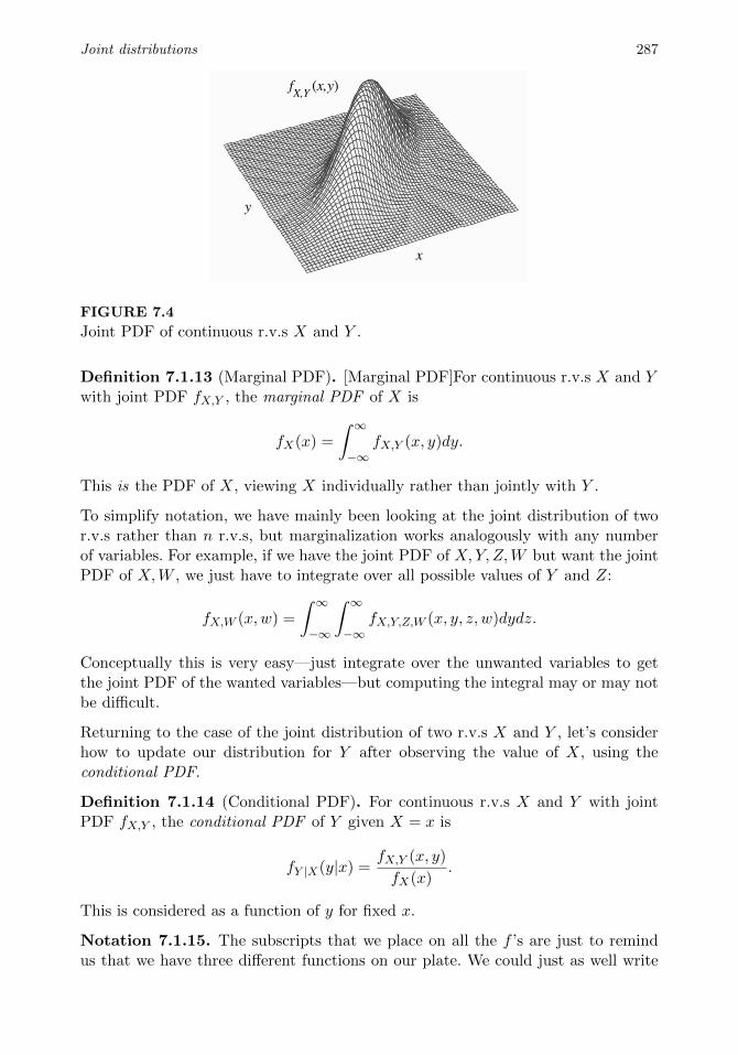
Joint distributions 287
x
y
fX,Y (x,y)
FIGURE 7.4
Joint PDF of continuous r.v.s X and Y .
Definition 7.1.13 (Marginal PDF). [Marginal PDF]For continuous r.v.s X and Ywith joint PDF fX,Y , the marginal PDF of X is
fX(x) =
Z 1
�1fX,Y (x, y)dy.
This is the PDF of X, viewing X individually rather than jointly with Y .
To simplify notation, we have mainly been looking at the joint distribution of twor.v.s rather than n r.v.s, but marginalization works analogously with any numberof variables. For example, if we have the joint PDF of X,Y, Z,W but want the jointPDF of X,W , we just have to integrate over all possible values of Y and Z:
fX,W (x,w) =
Z 1
�1
Z 1
�1fX,Y,Z,W (x, y, z, w)dydz.
Conceptually this is very easy—just integrate over the unwanted variables to getthe joint PDF of the wanted variables—but computing the integral may or may notbe di�cult.
Returning to the case of the joint distribution of two r.v.s X and Y , let’s considerhow to update our distribution for Y after observing the value of X, using theconditional PDF.
Definition 7.1.14 (Conditional PDF). For continuous r.v.s X and Y with jointPDF fX,Y , the conditional PDF of Y given X = x is
fY |X(y|x) = fX,Y (x, y)
fX(x).
This is considered as a function of y for fixed x.
Notation 7.1.15. The subscripts that we place on all the f ’s are just to remindus that we have three di↵erent functions on our plate. We could just as well write

288 Introduction to Probability
g(y|x) = f(x, y)/h(x), where f is the joint PDF, h is the marginal PDF of X, andg is the conditional PDF of Y given X = x, but that makes it more di�cult toremember which letter stands for which function.
Figure 7.5 illustrates the definition of conditional PDF. We take a vertical slice ofthe joint PDF corresponding to the observed value of X; since the total area underthis slice is fX(x), we then divide by fX(x) to ensure that the conditional PDFwill have an area of 1. Therefore conditional PDFs satisfy the properties of a validPDF.
X = x renormaliz
e
FIGURE 7.5
Conditional PDF of Y given X = x. The conditional PDF fY |X(y|x) is obtained byrenormalizing the slice of the joint PDF at the fixed value x.
h 7.1.16. How can we speak of conditioning on X = x for X a continuous r.v.,considering that this event has probability 0? Rigorously speaking, we are actuallyconditioning on the event thatX falls within a small interval of x, sayX 2 (x�✏, x+✏), and then taking a limit as ✏ approaches 0. We will not fuss over this technicality;fortunately, many important results such as Bayes’ rule work in the continuous caseexactly as one would hope.
Note that we can recover the joint PDF fX,Y if we have the conditional PDF fY |Xand the corresponding marginal fX :
fX,Y (x, y) = fY |X(y|x)fX(x).
Similarly, we can recover the joint PDF if we have fX|Y and fY :
fX,Y (x, y) = fX|Y (x|y)fY (y).
This allows us to develop continuous analogs of Bayes’ rule
P (Y = y|X = x) =P (X = x|Y = y)P (Y = y)
P (X = x)
and LOTPP (X = x) =
X
y
P (X = x|Y = y)P (Y = y).

Joint distributions 289
These formulas still hold in the continuous case, replacing probabilities with prob-ability density functions.
Theorem 7.1.17 (Continuous form of Bayes’ rule and LOTP). For continuous r.v.sX and Y ,
fY |X(y|x) =fX|Y (x|y)fY (y)
fX(x),
fX(x) =
Z 1
�1fX|Y (x|y)fY (y)dy.
Proof. By definition of conditional PDFs, we have
fY |X(y|x)fX(x) = fX,Y (x, y) = fX|Y (x|y)fY (y).
The continuous version of Bayes’ rule follows immediately from dividing by fX(x).The continuous version of LOTP follows immediately from integrating with respectto y:
fX(x) =
Z 1
�1fX,Y (x, y)dy =
Z 1
�1fX|Y (x|y)fY (y)dy.
⌅
Out of curiosity, let’s see what would have happened if we had plugged in the otherexpression for fX,Y (x, y) instead in the proof of LOTP:
fX(x) =
Z 1
�1fX,Y (x, y)dy =
Z 1
�1fY |X(y|x)fX(x)dy = fX(x)
Z 1
�1fY |X(y|x)dy.
So this just says that Z 1
�1fY |X(y|x)dy = 1,
confirming the fact that conditional PDFs must integrate to 1.
We now have versions of Bayes’ rule and LOTP for two discrete r.v.s and for two con-tinuous r.v.s. Better yet, there are also versions when we have one discrete r.v. andone continuous r.v. After understanding of the discrete versions, it is easy to re-member and use the other versions since they are analogous, replacing probabilitiesby PDFs when appropriate. Here are the four versions of Bayes’ rule, summarizedin a table.
Y discrete Y continuous
X discrete P (Y = y|X = x) = P (X=x|Y =y)P (Y =y)P (X=x)
fY (y|X = x) = P (X=x|Y =y)fY
(y)P (X=x)
X continuous P (Y = y|X = x) = fX
(x|Y =y)P (Y =y)fX
(x)fY |X(y|x) = f
X|Y (x|y)fY
(y)
fX
(x)
And here are the four versions of LOTP, summarized in a table.

290 Introduction to Probability
Y discrete Y continuous
X discrete P (X = x) =Py
P (X = x|Y = y)P (Y = y) P (X = x) =R1�1 P (X = x|Y = y)fY (y)dy
X continuous fX(x) =Py
fX(x|Y = y)P (Y = y) fX(x) =R1�1 fX|Y (x|y)fY (y)dy
Finally, let’s discuss the definition of independence for continuous r.v.s; then we’llturn to concrete examples. As in the discrete case, we can view independence ofcontinuous r.v.s in two ways. One is that the joint CDF factors into the productof the marginal CDFs, or the joint PDF factors into the product of the marginalPDFs. The other is that the conditional PDF of Y given X = x is the same as themarginal PDF of Y , so conditioning on X provides no information about Y .
Definition 7.1.18 (Independence of continuous r.v.s). Random variables X andY are independent if for all x and y,
FX,Y (x, y) = FX(x)FY (y).
If X and Y are continuous with joint PDF fX,Y , this is equivalent to the condition
fX,Y (x, y) = fX(x)fY (y)
for all x and y, and it is also equivalent to the condition
fY |X(y|x) = fY (y)
for all y and all x such that fX(x) > 0.
h 7.1.19. The marginal PDF of Y , fY (y), is a function of y only; it cannot dependon x in any way. The conditional PDF fY |X(y|x) can depend on x in general. Onlyin the special case of independence is fY |X(y|x) free of x.
Sometimes we have a joint PDF for X and Y that factors as a function of xtimes a function of y, without knowing in advance whether these functions are themarginal PDFs, or even whether they are valid PDFs. The next result addressesthis case.
Proposition 7.1.20. Suppose that the joint PDF fX,Y of X and Y factors as
fX,Y (x, y) = g(x)h(y)
for all x and y, where g and h are nonnegative functions. Then X and Y areindependent. Also, if either g or h is a valid PDF, then the other one is a valid PDFtoo and g and h are the marginal PDFs of X and Y , respectively. (The analogousresult in the discrete case also holds.)

Joint distributions 291
Proof. Let c =R1�1 h(y)dy. Multiplying and dividing by c, we can write
fX,Y (x, y) = cg(x) · h(y)c
.
(The point of this is that h(y)/c is a valid PDF.) Then the marginal PDF of X is
fX(x) =
Z 1
�1fX,Y (x, y)dy = cg(x)
Z 1
�1
h(y)
cdy = cg(x).
It follows thatR1�1 cg(x)dx = 1 since a marginal PDF is a valid PDF (knowing the
integral of h gave us the integral of g for free!). Then the marginal PDF of Y is
fY (y) =
Z 1
�1fX,Y (x, y)dx =
h(y)
c
Z 1
�1cg(x)dx =
h(y)
c.
Thus, X and Y are independent with PDFs cg(x) and h(y)/c, respectively. If g orh is already a valid PDF, then c = 1, so the other one is also a valid PDF. ⌅
h 7.1.21. In the above proposition, we need the joint PDF to factor as a functionof x times a function of y for all (x, y) in the plane R2, not just for (x, y) withfX,Y (x, y) > 0. The reason for this is illustrated in the next example.
A simple case of a continuous joint distribution is when the joint PDF is constantover some region in the plane. In the following example, we’ll compare a joint PDFthat is constant on a square to a joint PDF that is constant on a disk.
Example 7.1.22 (Uniform on a region in the plane). Let (X,Y ) be a completelyrandom point in the square {(x, y) : x, y 2 [0, 1]}, in the sense that the joint PDFof X and Y is constant over the square and 0 outside of it:
fX,Y (x, y) =
8><
>:
1 if x, y 2 [0, 1],
0 otherwise.
The constant 1 is chosen so that the joint PDF will integrate to 1. This distributionis called the Uniform distribution on the square.
Intuitively, it makes sense that X and Y should be Unif(0, 1) marginally. We cancheck this by computing
fX(x) =
Z1
0
fX,Y (x, y)dy =
Z1
0
1dy = 1,
and similarly for fY . Furthermore, X and Y are independent, since the joint PDFfactors into the product of the marginal PDFs (this just reduces to 1 = 1 · 1, butit’s important to note that the value of X does not constrain the possible values ofY ). So the conditional distribution of Y given X = x is Unif(0, 1), regardless of x.
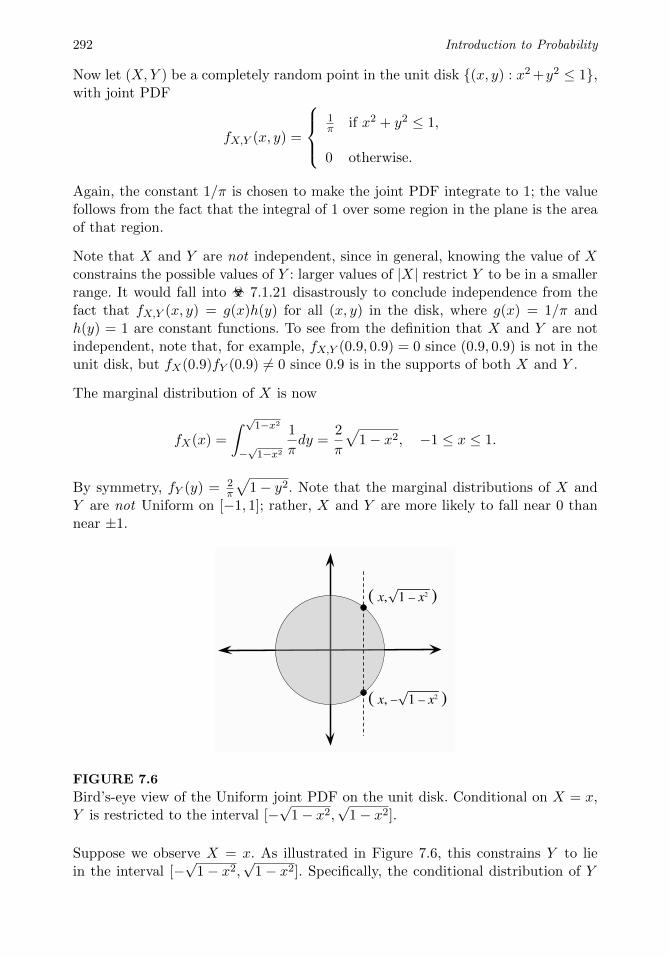
292 Introduction to Probability
Now let (X,Y ) be a completely random point in the unit disk {(x, y) : x2+y2 1},with joint PDF
fX,Y (x, y) =
8><
>:
1
⇡ if x2 + y2 1,
0 otherwise.
Again, the constant 1/⇡ is chosen to make the joint PDF integrate to 1; the valuefollows from the fact that the integral of 1 over some region in the plane is the areaof that region.
Note that X and Y are not independent, since in general, knowing the value of Xconstrains the possible values of Y : larger values of |X| restrict Y to be in a smallerrange. It would fall into h 7.1.21 disastrously to conclude independence from thefact that fX,Y (x, y) = g(x)h(y) for all (x, y) in the disk, where g(x) = 1/⇡ andh(y) = 1 are constant functions. To see from the definition that X and Y are notindependent, note that, for example, fX,Y (0.9, 0.9) = 0 since (0.9, 0.9) is not in theunit disk, but fX(0.9)fY (0.9) 6= 0 since 0.9 is in the supports of both X and Y .
The marginal distribution of X is now
fX(x) =
Z p1�x2
�p1�x2
1
⇡dy =
2
⇡
p1� x2, �1 x 1.
By symmetry, fY (y) =2
⇡
p1� y2. Note that the marginal distributions of X and
Y are not Uniform on [�1, 1]; rather, X and Y are more likely to fall near 0 thannear ±1.
( x,√1 – x2 )
( x, –√1 – x2 )
FIGURE 7.6
Bird’s-eye view of the Uniform joint PDF on the unit disk. Conditional on X = x,Y is restricted to the interval [�
p1� x2,
p1� x2].
Suppose we observe X = x. As illustrated in Figure 7.6, this constrains Y to liein the interval [�
p1� x2,
p1� x2]. Specifically, the conditional distribution of Y

Joint distributions 293
given X = x is
fY |X(y|x) = fX,Y (x, y)
fX(x)=
1
⇡2
⇡
p1� x2
=1
2p1� x2
for �p1� x2 y
p1� x2, and 0 otherwise. This conditional PDF is constant
as a function of y, which tells us that the conditional distribution of Y is Uniformon the interval [�
p1� x2,
p1� x2]. The fact that the conditional PDF is not free
of x confirms the fact that X and Y are not independent.
In general, for a region R in the plane, the Uniform distribution on R is defined tohave joint PDF that is constant inside R and 0 outside R. As above, the constant isthe reciprocal of the area of R. If R is the rectangle {(x, y) : a x b, c y d},then X and Y will be independent; unlike for a disk, the vertical slices of a rectangleall look the same. A way to generate a random (X,Y ) would then be to drawX ⇠ Unif(a, b) and Y ⇠ Unif(c, d) independently. But for any region where thevalue of X constrains the possible values of Y or vice versa, X and Y will not beindependent. ⇤As another example of working with joint PDFs, let’s consider a question that comesup often when dealing with Exponentials of di↵erent rates.
Example 7.1.23 (Comparing Exponentials of di↵erent rates). Let T1
⇠ Expo(�1
)and T
2
⇠ Expo(�2
) be independent. Find P (T1
< T2
). For example, T1
could bethe lifetime of a refrigerator and T
2
could be the lifetime of a stove (if we arewilling to assume Exponential distributions for these), and then P (T
1
< T2
) is theprobability that the refrigerator fails before the stove. We know from Chapter 5 thatmin(T
1
, T2
) ⇠ Expo(�1
+ �2
), which tells us about when the first appliance failurewill occur, but we also may want to know about which appliance will fail first.
Solution:
We just need to integrate the joint PDF of T1
and T2
over the appropriate region,which is all (t
1
, t2
) with t1
> 0, t2
> 0, and t1
< t2
. This yields
P (T1
< T2
) =
Z 1
0
Z t2
0
�1
e��1
t1�
2
e��2
t2dt
1
dt2
=
Z 1
0
✓Z t2
0
�1
e��1
t1dt
1
◆�2
e��2
t2dt
2
=
Z 1
0
(1� e��1
t2)�
2
e��2
t2dt
2
= 1�Z 1
0
�2
e�(�1
+�2
)t2dt
2
= 1� �2
�1
+ �2
=�1
�1
+ �2
.

294 Introduction to Probability
To get from the first line to the second, we took out �2
e��2
t2 from the inner integral
since it is treated as a constant when integrating with respect to t1
.
This result makes sense intuitively if we interpret �1
and �2
as rates. For example,if refrigerators have twice the failure rate of stoves, then it says that the odds are 2to 1 in favor of the refrigerator failing first. As a simple check, note that the answerreduces to 1/2 when �
1
= �2
(in that case, we already knew P (T1
< T2
) = 1/2 bysymmetry).
An alternative method of getting the same result is to use LOTP to condition onT1
(or condition on T2
). A third approach is in Chapter 13, which relates this resultto Poisson processes and proves it using the bank–post o�ce story. ⇤
Our last example in this section demonstrates how we can use the joint distributionof X and Y to derive the distribution of a function of X and Y .
Example 7.1.24 (Cauchy PDF). Let X and Y be i.i.d. N (0, 1), and let T = X/Y .The distribution of T is a famous named distribution called the Cauchy distribution,and we will encounter it again in Chapter 10. Meanwhile, find the PDF of T .
Solution:
We’ll find the CDF of T first and di↵erentiate to get the PDF. We can write
FT (t) = P (T t) = P
✓X
Y t
◆= P
✓X
|Y | t
◆,
since the r.v.s XY and X
|Y | are identically distributed by the symmetry of the standard
Normal distribution. Now |Y | is nonnegative, so we can multiply by it on both sideswithout reversing the direction of the inequality. Thus, we are interested in finding
FT (t) = P (X t|Y |).
We calculate this probability by integrating the joint PDF of X and Y over theregion where X t|Y | holds. The joint PDF of X and Y is just the product of themarginal PDFs, by independence. So
FT (t) = P (X t|Y |)
=
Z 1
�1
Z t|y|
�1
1p2⇡
e�x2/2 1p2⇡
e�y2/2dxdy.
Note that the inner limits of integration (the limits for x) depend on y, whereasthe outer limits of integration (the limits for y) can’t depend on x (see the mathappendix for more about limits of integration with multiple integrals). With some

Joint distributions 295
manipulations, we can get the double integral down to a single integral:
FT (t) =
Z 1
�1
1p2⇡
e�y2/2
Z t|y|
�1
1p2⇡
e�x2/2dx
!dy
=
Z 1
�1
1p2⇡
e�y2/2�(t|y|)dy
=
r2
⇡
Z 1
0
e�y2/2�(ty)dy.
Alternatively, we can get the same result without doing a double integral by usingone of the versions of LOTP. Letting I be the indicator r.v. for the event X t|Y |,we again have
P (I = 1) =
Z 1
�1P (I = 1|Y = y)fY (y)dy
=
Z 1
�1
1p2⇡
e�y2/2�(t|y|)dy.
At this point we seem to be stuck with an integral we don’t know how to do.Fortunately, we were asked to find the PDF, not the CDF, so instead of evaluatingthe integral, we can just di↵erentiate it with respect to t (not with respect to y, whichis a dummy variable). We are permitted to interchange the order of integration anddi↵erentiation under mild technical conditions, which are met here. This gives
fT (t) = F 0T (t) =
r2
⇡
Z 1
0
d
dt
⇣e�y2/2�(ty)
⌘dy
=
r2
⇡
Z 1
0
ye�y2/2'(ty)dy
=1
⇡
Z 1
0
ye�(1+t
2
)y
2
2 dy
=1
⇡(1 + t2),
using the substitution u = (1 + t2)y2/2, du = (1 + t2)ydy for the final step. So thePDF of T is
fT (t) =1
⇡(1 + t2), t 2 R.
Since Z 1
�1
1
1 + t2dt = tan�1(1)� tan�1(�1) = ⇡,
we have obtained a valid PDF. And if we do want the CDF, we can find that byintegrating the PDF over the appropriate interval.
As we mentioned, the distribution of T is called the Cauchy distribution. TheCauchy PDF is similar in shape to the Normal bell curve, but with tails that decay
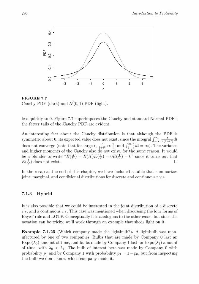
296 Introduction to Probability
−3 −2 −1 0 1 2 3
0.0
0.1
0.2
0.3
0.4
x
FIGURE 7.7
Cauchy PDF (dark) and N (0, 1) PDF (light).
less quickly to 0. Figure 7.7 superimposes the Cauchy and standard Normal PDFs;the fatter tails of the Cauchy PDF are evident.
An interesting fact about the Cauchy distribution is that although the PDF issymmetric about 0, its expected value does not exist, since the integral
R1�1
t⇡(1+t2)dt
does not converge (note that for large t, t1+t2 ⇡ 1
t , andR11
1
t dt = 1). The varianceand higher moments of the Cauchy also do not exist, for the same reason. It wouldbe a blunder to write “E(XY ) = E(X)E( 1
Y ) = 0E( 1
Y ) = 0” since it turns out thatE( 1
Y ) does not exist. ⇤
In the recap at the end of this chapter, we have included a table that summarizesjoint, marginal, and conditional distributions for discrete and continuous r.v.s.
7.1.3 Hybrid
It is also possible that we could be interested in the joint distribution of a discreter.v. and a continuous r.v. This case was mentioned when discussing the four forms ofBayes’ rule and LOTP. Conceptually it is analogous to the other cases, but since thenotation can be tricky, we’ll work through an example that sheds light on it.
Example 7.1.25 (Which company made the lightbulb?). A lightbulb was man-ufactured by one of two companies. Bulbs that are made by Company 0 last anExpo(�
0
) amount of time, and bulbs made by Company 1 last an Expo(�1
) amountof time, with �
0
< �1
. The bulb of interest here was made by Company 0 withprobability p
0
and by Company 1 with probability p1
= 1� p0
, but from inspectingthe bulb we don’t know which company made it.

Joint distributions 297
Let T be how long the bulb lasts, and I be the indicator of it having been made byCompany 1.
(a) Find the CDF and PDF of T .
(b) Does T have the memoryless property?
(c) Find the conditional distribution of I given T = t. What happens to this ast ! 1?
Solution:
Since T is a continuous r.v. and I is discrete, the joint distribution of T and I is ahybrid, as illustrated in Figure 7.8. In a joint PDF of two continuous r.v.s, there areinfinitely many vertical slices of the joint PDF that we can take, each correspondingto a di↵erent conditional PDF. Here there are only two conditional PDFs of T , onefor I = 0 and one for I = 1. As stated in the problem, the conditional distribution ofT given I = 0 is Expo(�
0
) and given I = 1 is Expo(�1
). The marginal distributionof I is Bern(p
1
).
I = 0I = 1 t
FIGURE 7.8
Hybrid joint distribution of T and I.
Thus, we are given the joint distribution of T and I in terms of (1) the marginaldistribution of I and (2) the conditional distribution of T given I. The problemthen asks us to flip it around and find (1) the marginal distribution of T and (2)the conditional distribution of I given T . Phrased in this way, it becomes clear thatLOTP and Bayes’ rule will be our friends.
(a) In this part we are asked to derive the marginal distribution of T . For the CDF,we use the law of total probability, conditioning on I:
FT (t) = P (T t) = P (T t|I = 0)p0
+ P (T t|I = 1)p1
= (1� e��0
t)p0
+ (1� e��1
t)p1
= 1� p0
e��0
t � p1
e��1
t

298 Introduction to Probability
for t > 0. The marginal PDF is the derivative of the CDF:
fT (t) = p0
�0
e��0
t + p1
�1
e��1
t, for t > 0.
We could also have gotten this directly from the “X continuous, Y discrete” versionof LOTP, but we did not write out a proof of that version of LOTP, and workingthrough this example helps show why that version of LOTP works.
(b) Since �0
6= �1
, the above expression for the PDF does not reduce to the form�e��t. So the distribution of T is not Exponential, which implies that it does nothave the memoryless property. (The distribution of T is called a mixture of twoExponentials.)
(c) Using a hybrid form of Bayes’ rule, which is the “X continuous, Y discrete”version in the table of versions of Bayes’ rule, we have
P (I = 1|T = t) =fT (t|I = 1)P (I = 1)
fT (t),
where fT (t|I = 1) is the conditional PDF of T given I = 1, evaluated at t. Usingthe fact that T |I = 1 ⇠ Expo(�
1
) and the marginal PDF derived in (a),
P (I = 1|T = t) =p1
�1
e��1
t
p0
�0
e��0
t + p1
�1
e��1
t=
p1
�1
p0
�0
e(�1
��0
)t + p1
�1
.
Thus the conditional distribution of I given T = t is Bernoulli with this probabilityof success. This probability goes to 0 as t ! 1, which makes sense intuitively: thelonger the bulb lasts, the more confident we will be that it was made by Company0, as their bulbs have a lower failure rate � and a higher life expectancy 1
� . ⇤
7.2 2D LOTUS
The two-dimensional version of LOTUS lets us calculate the expectation of a ran-dom variable that is a function of two random variables X and Y , using the jointdistribution of X and Y .
Theorem 7.2.1 (2D LOTUS). Let g be a function from R2 to R. If X and Y arediscrete, then
E(g(X,Y )) =X
x
X
y
g(x, y)P (X = x, Y = y).
If X and Y are continuous with joint PDF fX,Y , then
E(g(X,Y )) =
Z 1
�1
Z 1
�1g(x, y)fX,Y (x, y)dxdy.

Joint distributions 299
Like its 1D counterpart, 2D LOTUS saves us from having to find the distributionof g(X,Y ) in order to calculate its expectation. Instead, having the joint PMF orjoint PDF of X and Y is enough.
One use of 2D LOTUS is to find the expected distance between two random vari-ables. For example, we can find the expected distance between two i.i.d. Uniformr.v.s or two i.i.d. standard Normal r.v.s.
Example 7.2.2 (Expected distance between two Uniforms). For X,Yi.i.d.⇠
Unif(0, 1), find E(|X � Y |).
Solution:
Since the joint PDF equals 1 on the unit square {(x, y) : x, y 2 [0, 1]}, 2D LOTUSgives
E(|X � Y |) =Z
1
0
Z1
0
|x� y|dxdy
=
Z1
0
Z1
y(x� y)dxdy +
Z1
0
Z y
0
(y � x)dxdy
= 2
Z1
0
Z1
y(x� y)dxdy = 1/3.
First we broke up the integral into two parts so we could eliminate the absolutevalue; then we used symmetry.
Incidentally, by solving this problem, we have also figured out the expected valueof M = max(X,Y ) and L = min(X,Y ). Since M +L is the same r.v. as X +Y andM � L is the same r.v. as |X � Y |,
E(M + L) = E(X + Y ) = 1,
E(M � L) = E(|X � Y |) = 1/3.
This is a system of two equations and two unknowns, which we can solve to getE(M) = 2/3 and E(L) = 1/3. As a check, E(M) exceeds E(L), as it should, andE(M) and E(L) are equidistant from 1/2, as should be the case due to symmetry.
⇤Example 7.2.3 (Expected distance between two Normals). For X,Y
i.i.d.⇠ N (0, 1),find E(|X � Y |).
Solution:
We could again use 2D LOTUS, giving
E(|X � Y |) =Z 1
�1
Z 1
�1|x� y| 1p
2⇡e�x2/2 1p
2⇡e�y2/2dxdy,
but an easier solution uses the fact that the sum or di↵erence of independent Nor-mals is Normal, as we proved using MGFs in Chapter 6. Then X �Y ⇠ N (0, 2), so

300 Introduction to Probability
we can write X � Y =p2Z where Z ⇠ N (0, 1), and E(|X � Y |) =
p2E|Z|. Now
we’ve reduced a 2D LOTUS to a 1D LOTUS:
E|Z| =Z 1
�1|z| 1p
2⇡e�z2/2dz = 2
Z 1
0
z1p2⇡
e�z2/2dz =
r2
⇡,
so E(|X � Y |) = 2p⇡. ⇤
We can also use 2D LOTUS to give another proof of linearity of expectation.
Example 7.2.4 (Linearity via 2D LOTUS). Let X and Y be continuous r.v.s (theanalogous method also works in the discrete case). By 2D LOTUS,
E(X + Y ) =
Z 1
�1
Z 1
�1(x+ y)fX,Y (x, y)dxdy
=
Z 1
�1
Z 1
�1xfX,Y (x, y)dxdy +
Z 1
�1
Z 1
�1yfX,Y (x, y)dxdy.
= E(X) + E(Y ).
This is a short proof of linearity of expectation. For the last step, we used 2D LOTUSand the fact that X is a function of X and Y (that happens to be degenerate in thesense that it doesn’t involve X), and similarly for Y . Another way to get the laststep is to writeZ 1
�1
Z 1
�1yfX,Y (x, y)dxdy =
Z 1
�1y
Z 1
�1fX,Y (x, y)dxdy =
Z 1
�1yfY (y)dy = E(Y ),
where we took y out from the inner integral (since y is held constant when integrat-ing with respect to x) and then recognized the marginal PDF of Y . For the E(X)term we can first swap the order of integration, from dxdy to dydx, and then thesame argument that we used for the E(Y ) term can be applied. ⇤
7.3 Covariance and correlation
Just as the mean and variance provided single-number summaries of the distributionof a single r.v., covariance is a single-number summary of the joint distribution oftwo r.v.s. Roughly speaking, covariance measures a tendency of two r.v.s to go upor down together, relative to their expected values: positive covariance betweenX and Y indicates that when X goes up, Y also tends to go up, and negativecovariance indicates that when X goes up, Y tends to go down. Here is the precisedefinition.
Definition 7.3.1 (Covariance). The covariance between r.v.s X and Y is
Cov(X,Y ) = E((X � EX)(Y � EY )).

Joint distributions 301
Multiplying this out and using linearity, we have an equivalent expression:
Cov(X,Y ) = E(XY )� E(X)E(Y ).
Let’s think about the definition intuitively. If X and Y tend to move in the samedirection, then X � EX and Y � EY will tend to be either both positive or bothnegative, so (X � EX)(Y � EY ) will be positive on average, giving a positivecovariance. If X and Y tend to move in opposite directions, then X � EX andY � EY will tend to have opposite signs, giving a negative covariance.
If X and Y are independent, then their covariance is zero. We say that r.v.s withzero covariance are uncorrelated.
Theorem 7.3.2. If X and Y are independent, then they are uncorrelated.
Proof. We’ll show this in the case where X and Y are continuous, with PDFs fXand fY . Since X and Y are independent, their joint PDF is the product of themarginal PDFs. By 2D LOTUS,
E(XY ) =
Z 1
�1
Z 1
�1xyfX(x)fY (y)dxdy
=
Z 1
�1yfY (y)
✓Z 1
�1xfX(x)dx
◆dy
=
Z 1
�1xfX(x)dx
Z 1
�1yfY (y)dy
= E(X)E(Y ).
The proof in the discrete case is the same, with PMFs instead of PDFs. ⌅
The converse of this theorem is false: just because X and Y are uncorrelated doesnot mean they are independent. For example, let X ⇠ N (0, 1), and let Y = X2.Then E(XY ) = E(X3) = 0 because the odd moments of the standard Normaldistribution are equal to 0 by symmetry. Thus X and Y are uncorrelated,
Cov(X,Y ) = E(XY )� E(X)E(Y ) = 0� 0 = 0,
but they are certainly not independent: Y is a function of X, so knowing X gives usperfect information about Y . Covariance is a measure of linear association, so r.v.scan be dependent in nonlinear ways and still have zero covariance, as this exampledemonstrates. The bottom right plot of Figure 7.9 shows draws from the jointdistribution of X and Y in this example. The other three plots illustrate positivecorrelation, negative correlation, and independence.
Covariance has the following key properties.
1. Cov(X,X) = Var(X).
2. Cov(X,Y ) = Cov(Y,X).

302 Introduction to Probability
●
●
●
●
●
●
●
●
●
●
●
●
●
●
●
●
●
●
●
●
●●
●
●
●
●
●
●
●●
●
●
●
● ●
●
●●
●
●
●
●
●
●
●
●
●
●
●
●
●
●●
●
●●
●
●
●
●
●
●
●
●●
●
●
●
●
●
●
● ●
●
●
●
●
●
●
●
●
●
●
●
●
●
●
●
●
●
●
●
●
●
●
●●
●
●
●
●
●
●
●
●
●
●
●
●
●
●
●
●
●
●●
●
●
●
●
●
●
●
●
●
●●
●
●
●
●
●
●
●
●
●
●
●
●
●
●●
● ●
●
●
●
●
●
●
●
●
●
●
●
●
●
●
●
●
●
●●
●
●
●
●
●
●
●
●
●●
●
●
●
●
●
●
●
●
●
●
●●
●
●
●
●
●
●
●
●
●
●
●
●
●
●
●
−3 −2 −1 0 1 2 3
−3−2
−10
12
3
Positive correlation
x
y
●●
●
●
●
●●
●
●
●●
●
●
●
●
●●
●
●
●
●
●
●
●
●
●
●
●
●
●
●
●
●
●
●
●
● ●
●●
●●
●
●
●
●
●
●
●
● ●
●
●
●
●
●
●
●
●
●
●
●●
●
●
●
●
●
●
●
●
●
●
●
●
●
●
●
● ●
●
●
●
●
● ●●
●
●●
●
●
●●
●
●
●
●
●
●
●●
●
●
●
●
●
●
●
●
●
●
●
●
●
●
●
●
●
●
●
●
●
●
●
●●
●
●
●
●
●
●
●
●
●
●
●
●
●
●
●
●
●
●
●
●
●
●●
●
●
●
●
●
●
●
●
●
●
●
●
●
●●
●
●
●
●
●
●
●
●
●
●
●
●
●
●
●
●
●
●
●
●
●
●
●●
●
●●
●
●
●
●
●
●
●
●
−3 −2 −1 0 1 2 3
−3−2
−10
12
3
Negative correlation
x
y
●
●
●●
●
●
●
●
●
●
●
●
●
●
●
●
●
●
●
●
●
●
●
●
●
●
●
●
●
●
●●
●
●
●●
●
●
●
●
●
●●
●
●
●
●
●
●
●
●
●
●
●
●
●
●
●
●
●
●●
●
●
●
●
●
●
●
●
●
●
●
●
●
●
●
●
●
●
●
●
●
●
●
●
●
●
●
●
●
●
●
●
●
●
●
●
●
●
●
●
●
●
●
●
●
●
●
●
●
●
●
●
●
●
●
●
●
●
●
●
●
●
●
●
●
●
●
●
●
●
●
●
●
●●
●
●
●
●
●
●
●
●
●
●
●
●
●
●
●
●
●
●
●
●
●
●
●
● ●
●
● ●
●
●
●
●
●
●
●
●
●
●
●
●
●
●
●
●●
●
●
●
●
●
●●
●●
●
●
●
●
●
●
●
●
●
−3 −2 −1 0 1 2 3
−3−2
−10
12
3
Independent
x
y
●
●
●
●
●
●
●●
●●●
●
●
●
●
●
● ●
●
●
●
●
●
●
●
●
●
●
●
●●
●
● ●
●
●
●●
●
●●
●●
●●
●●
●
●
●
●
●●
●
●
●
●
●
●
●
●
●
●
●●
●
●
●
●
●
●
●
●
●
●
●
●
●
●
●
●
●
●
●
●
●
●
●●
●
●
●
●
●
●
●
●●
●●
●●
●
●
●
●
●●●
●
●
●
●
●●
●●
●
●
● ● ●●
●
●●
● ●
●
●
●
●
●
●●
●
●
●●
●
●●
●
●●●
●
●
●
●
●
●
●
●
●
● ●●
●
●
●
●
●
●
●
●
●
●
●●
●●
●
●
●
●
●
●
●
●●
●
●
●
●
● ●●
●
●
●
●●
●
●
●
●●
●
●
−3 −2 −1 0 1 2 3
02
46
Dependent but uncorrelated
x
y
FIGURE 7.9
Draws from the joint distribution of (X,Y ) under various dependence structures.Top left: X and Y are positively correlated. Top right: X and Y are negativelycorrelated. Bottom left: X and Y are independent, hence uncorrelated. Bottomright: Y is a deterministic function of X, but X and Y are uncorrelated.

Joint distributions 303
3. Cov(X, c) = 0 for any constant c.
4. Cov(aX, Y ) = aCov(X,Y ) for any constant a.
5. Cov(X + Y, Z) = Cov(X,Z) + Cov(Y, Z).
6. Cov(X + Y, Z +W ) = Cov(X,Z) +Cov(X,W ) +Cov(Y, Z) +Cov(Y,W ).
7. Var(X + Y ) = Var(X) + Var(Y ) + 2Cov(X,Y ). For n r.v.s X1
, . . . , Xn,
Var(X1
+ · · ·+Xn) = Var(X1
) + · · ·+Var(Xn) + 2X
i<j
Cov(Xi, Xj).
The first five properties follow readily from the definition and basic properties ofexpectation. Property 6 follows from Property 2 and Property 5, by expanding
Cov(X + Y, Z +W ) = Cov(X,Z +W ) + Cov(Y, Z +W )
= Cov(Z +W,X) + Cov(Z +W,Y )
= Cov(Z,X) + Cov(W,X) + Cov(Z, Y ) + Cov(W,Y )
= Cov(X,Z) + Cov(X,W ) + Cov(Y, Z) + Cov(Y,W ).
Property 7 follows from writing the variance of an r.v. as its covariance with itself(by Property 1) and then using Property 6 repeatedly. We have now fulfilled ourpromise from Chapter 4 that for independent r.v.s, the variance of the sum is thesum of the variances. By Theorem 7.3.2, independent r.v.s are uncorrelated, so inthat case all the covariance terms drop out of the expression in Property 7.
h 7.3.3. If X and Y are independent, then the properties of covariance give
Var(X � Y ) = Var(X) + Var(�Y ) = Var(X) + Var(Y ).
It is a common mistake to claim “Var(X�Y ) = Var(X)�Var(Y )”; this is a categoryerror since Var(X)�Var(Y ) could be negative. For general X and Y , we have
Var(X � Y ) = Var(X) + Var(Y )� 2Cov(X,Y ).
Since covariance depends on the units in which X and Y are measured—if we de-cide to measure X in centimeters rather than meters, the covariance is multiplieda hundredfold—it is easier to interpret a unitless version of covariance called corre-lation.
Definition 7.3.4 (Correlation). The correlation between r.v.s X and Y is
Corr(j, Y ) =Cov(X,Y )pVar(X)Var(Y )
.
(This is undefined in the degenerate cases Var(X) = 0 or Var(Y ) = 0.)

304 Introduction to Probability
Notice that shifting and scaling X and Y has no e↵ect on their correlation. Shiftingdoes not a↵ect Cov(X,Y ), Var(X), or Var(Y ), so the correlation is unchanged. Asfor scaling, the fact that we divide by the standard deviations of X and Y ensuresthat the scale factor cancels out:
Corr(cX, Y ) =Cov(cX, Y )pVar(cX)Var(Y )
=cCov(X,Y )p
c2Var(X)Var(Y )= Corr(X,Y ).
Correlation is convenient to interpret because it does not depend on the units ofmeasurement and is always between �1 and 1.
Theorem 7.3.5 (Correlation bounds). For any r.v.s X and Y ,
�1 Corr(X,Y ) 1.
Proof. Without loss of generality we can assume X and Y have variance 1, sincescaling does not change the correlation. Let ⇢ = Corr(X,Y ) = Cov(X,Y ). Usingthe fact that variance is nonnegative, along with Property 7 of covariance, we have
Var(X + Y ) = Var(X) + Var(Y ) + 2Cov(X,Y ) = 2 + 2⇢ � 0,
Var(X � Y ) = Var(X) + Var(Y )� 2Cov(X,Y ) = 2� 2⇢ � 0.
Thus, �1 ⇢ 1. ⌅
Here is an example of how to calculate correlation from the definition.
Example 7.3.6 (Exponential max and min). Let X and Y be i.i.d. Expo(1) r.v.s.Find the correlation between max(X,Y ) and min(X,Y ).
Solution:
Let M = max(X,Y ) and L = min(X,Y ). By the memoryless property and resultsfrom Chapter 5, we know that L ⇠ Expo(2), M � L ⇠ Expo(1), and M � L isindependent of L. To explain this in more detail, imagine that two students areindependently trying to solve a problem, and each takes an Expo(1) amount oftime to solve the problem (the Exponential distribution would not make sense ifthe problem is just busy-work or where steady progress can be made, but could be areasonable approximation if it is a hard problem that requires creative thinking). Attime L, one of the two students solves the problem. Now condition on L, and see howmuch longer it will take the other student to solve the problem. By the memorylessproperty, the additional time M � L is a fresh Expo(1) r.v., independent of L.
We now have
Cov(M,L) = Cov(M �L+L,L) = Cov(M �L,L) + Cov(L,L) = 0 +Var(L) =1
4,
Var(M) = Var(M � L+ L) = Var(M � L) + Var(L) = 1 +1
4=
5
4,
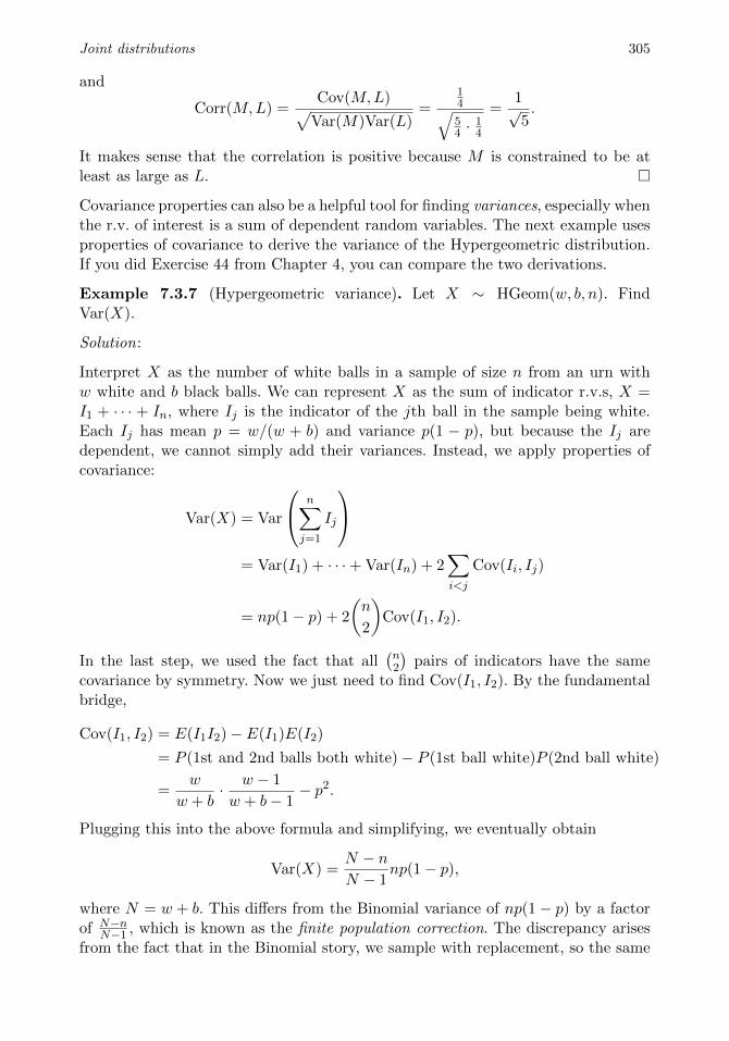
Joint distributions 305
and
Corr(M,L) =Cov(M,L)pVar(M)Var(L)
=1
4q5
4
· 1
4
=1p5.
It makes sense that the correlation is positive because M is constrained to be atleast as large as L. ⇤Covariance properties can also be a helpful tool for finding variances, especially whenthe r.v. of interest is a sum of dependent random variables. The next example usesproperties of covariance to derive the variance of the Hypergeometric distribution.If you did Exercise 44 from Chapter 4, you can compare the two derivations.
Example 7.3.7 (Hypergeometric variance). Let X ⇠ HGeom(w, b, n). FindVar(X).
Solution:
Interpret X as the number of white balls in a sample of size n from an urn withw white and b black balls. We can represent X as the sum of indicator r.v.s, X =I1
+ · · · + In, where Ij is the indicator of the jth ball in the sample being white.Each Ij has mean p = w/(w + b) and variance p(1 � p), but because the Ij aredependent, we cannot simply add their variances. Instead, we apply properties ofcovariance:
Var(X) = Var
0
@nX
j=1
Ij
1
A
= Var(I1
) + · · ·+Var(In) + 2X
i<j
Cov(Ii, Ij)
= np(1� p) + 2
✓n
2
◆Cov(I
1
, I2
).
In the last step, we used the fact that all�n2
�pairs of indicators have the same
covariance by symmetry. Now we just need to find Cov(I1
, I2
). By the fundamentalbridge,
Cov(I1
, I2
) = E(I1
I2
)� E(I1
)E(I2
)
= P (1st and 2nd balls both white)� P (1st ball white)P (2nd ball white)
=w
w + b· w � 1
w + b� 1� p2.
Plugging this into the above formula and simplifying, we eventually obtain
Var(X) =N � n
N � 1np(1� p),
where N = w + b. This di↵ers from the Binomial variance of np(1� p) by a factorof N�n
N�1
, which is known as the finite population correction. The discrepancy arisesfrom the fact that in the Binomial story, we sample with replacement, so the same

306 Introduction to Probability
ball can be drawn multiple times; in the Hypergeometric story, we sample withoutreplacement, so each ball appears in the sample at most once. If we consider N to bethe “population size” of the urn, then as N grows very large relative to the samplesize n, it becomes extremely unlikely that in sampling with replacement, we woulddraw the same ball more than once. Thus sampling with replacement and samplingwithout replacement become equivalent in the limit as N ! 1 with n fixed, andthe finite population correction approaches 1.
The other case where sampling with and without replacement are equivalent isthe simple case where we only draw one ball from the urn, and indeed, the finitepopulation correction also equals 1 when n = 1. ⇤The last two sections in this chapter introduce the Multinomial and the MultivariateNormal distributions. The Multinomial is the most famous discrete multivariate dis-tribution, and the Multivariate Normal is the most famous continuous multivariatedistribution.
7.4 Multinomial
The Multinomial distribution is a generalization of the Binomial. Whereas the Bi-nomial distribution counts the successes in a fixed number of trials that can only becategorized as success or failure, the Multinomial distribution keeps track of trialswhose outcomes can fall into multiple categories, such as excellent, adequate, poor;or red, yellow, green, blue.
Story 7.4.1 (Multinomial distribution). Each of n objects is independently placedinto one of k categories. An object is placed into category j with probability pj ,
where the pj are nonnegative andPk
j=1
pj = 1. Let X1
be the number of objects incategory 1, X
2
the number of objects in category 2, etc., so that X1
+ · · ·+Xk = n.ThenX = (X
1
, . . . , Xk) is said to have theMultinomial distribution with parametersn and p = (p
1
, . . . , pk). We write this as X ⇠ Multk(n,p). ⇤We call X a random vector because it is a vector of random variables. The jointPMF of X can be derived from the story.
Theorem 7.4.2 (Multinomial joint PMF). If X ⇠ Multk(n,p), then the joint PMFof X is
P (X1
= n1
, . . . , Xk = nk) =n!
n1
!n2
! . . . nk!· pn1
1
pn2
2
. . . pnk
k ,
for n1
, . . . , nk satisfying n1
+ · · ·+ nk = n.
Proof. If n1
, . . . , nk don’t add up to n, then the event {X1
= n1
, . . . , Xk = nk} isimpossible: every object has to go somewhere, and new objects can’t appear out ofnowhere. If n
1
, . . . , nk do add up to n, then any particular way of putting n1
objects
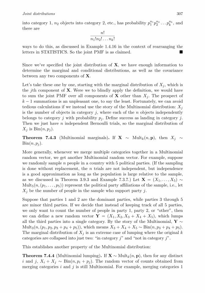
Joint distributions 307
into category 1, n2
objects into category 2, etc., has probability pn1
1
pn2
2
. . . pnk
k , andthere are
n!
n1
!n2
! . . . nk!
ways to do this, as discussed in Example 1.4.16 in the context of rearranging theletters in STATISTICS. So the joint PMF is as claimed. ⌅
Since we’ve specified the joint distribution of X, we have enough information todetermine the marginal and conditional distributions, as well as the covariancebetween any two components of X.
Let’s take these one by one, starting with the marginal distribution of Xj , which isthe jth component of X. Were we to blindly apply the definition, we would haveto sum the joint PMF over all components of X other than Xj . The prospect ofk � 1 summations is an unpleasant one, to say the least. Fortunately, we can avoidtedious calculations if we instead use the story of the Multinomial distribution: Xj
is the number of objects in category j, where each of the n objects independentlybelongs to category j with probability pj . Define success as landing in category j.Then we just have n independent Bernoulli trials, so the marginal distribution ofXj is Bin(n, pj).
Theorem 7.4.3 (Multinomial marginals). If X ⇠ Multk(n,p), then Xj ⇠Bin(n, pj).
More generally, whenever we merge multiple categories together in a Multinomialrandom vector, we get another Multinomial random vector. For example, supposewe randomly sample n people in a country with 5 political parties. (If the samplingis done without replacement, the n trials are not independent, but independenceis a good approximation as long as the population is large relative to the sample,as we discussed in Theorem 3.9.3 and Example 7.3.7.) Let X = (X
1
, . . . , X5
) ⇠Mult
5
(n, (p1
, . . . , p5
)) represent the political party a�liations of the sample, i.e., letXj be the number of people in the sample who support party j.
Suppose that parties 1 and 2 are the dominant parties, while parties 3 through 5are minor third parties. If we decide that instead of keeping track of all 5 parties,we only want to count the number of people in party 1, party 2, or “other”, thenwe can define a new random vector Y = (X
1
, X2
, X3
+ X4
+ X5
), which lumpsall the third parties into a single category. By the story of the Multinomial, Y ⇠Mult
3
(n, (p1
, p2
, p3
+ p4
+ p5
)), which means X3
+X4
+X5
⇠ Bin(n, p3
+ p4
+ p5
).The marginal distribution of Xj is an extreme case of lumping where the original kcategories are collapsed into just two: “in category j” and “not in category j”.
This establishes another property of the Multinomial distribution:
Theorem 7.4.4 (Multinomial lumping). If X ⇠ Multk(n,p), then for any distincti and j, Xi + Xj ⇠ Bin(n, pi + pj). The random vector of counts obtained frommerging categories i and j is still Multinomial. For example, merging categories 1

308 Introduction to Probability
FIGURE 7.10
Lumping categories in a Multinomial random vector produces another Multinomialrandom vector.
and 2 gives
(X1
+X2
, X3
, . . . , Xk) ⇠ Multk�1
(n, (p1
+ p2
, p3
, . . . , pn)).
Now for the conditional distributions. Suppose we get to observe X1
, the number ofobjects in category 1, and we wish to update our distribution for the other categories(X
2
, . . . , Xk). One way to do this is with the definition of conditional PMF:
P (X2
= n2
, . . . , Xk = nk|X1
= n1
) =P (X
1
= n1
, X2
= n2
, . . . , Xk = nk)
P (X1
= n1
).
The numerator is the joint PMF of the Multinomial, and the denominator is themarginal PMF of X
1
, both of which we have already derived. However, we preferto use the Multinomial story to deduce the conditional distribution of (X
2
, . . . , Xk)without algebra. Given that there are n
1
objects in category 1, the remaining n�n1
objects fall into categories 2 through k, independently of one another. By Bayes’rule, the conditional probability of falling into category j is
P (in category j|not in category 1) =P (in category j)
P (not in category 1)=
pjp2
+ · · ·+ pk,
for j = 2, . . . , k. This makes intuitive sense: the updated probabilities are pro-portional to the original probabilities (p
2
, . . . , pk), but these must be renormalizedto yield a valid probability vector. Putting it all together, we have the followingresult.
Theorem 7.4.5 (Multinomial conditioning). If X ⇠ Multk(n,p), then
(X2
, . . . , Xk)��X
1
= n1
⇠ Multk�1
(n� n1
, (p02
, . . . , p0k)),
where p0j = pj/(p2 + · · ·+ pk).

Joint distributions 309
Finally, we know that components within a Multinomial random vector are de-pendent since they are constrained by X
1
+ · · · + Xk = n. To find the covariancebetween Xi and Xj , we can use the marginal and lumping properties we have justdiscussed.
Theorem 7.4.6 (Covariance in a Multinomial). Let (X1
, . . . , Xk) ⇠ Multk(n,p),where p = (p
1
, . . . , pk). For i 6= j, Cov(Xi, Xj) = �npipj .
Proof. For concreteness, let i = 1 and j = 2. Using the lumping property andthe marginal distributions of a Multinomial, we know X
1
+ X2
⇠ Bin(n, p1
+ p2
),X
1
⇠ Bin(n, p1
), X2
⇠ Bin(n, p2
). Therefore
Var(X1
+X2
) = Var(X1
) + Var(X2
) + 2Cov(X1
, X2
)
becomes
n(p1
+ p2
)(1� (p1
+ p2
)) = np1
(1� p1
) + np2
(1� p2
) + 2Cov(X1
, X2
).
Solving for Cov(X1
, X2
) gives Cov(X1
, X2
) = �np1
p2
. By the same logic, for i 6= j,we have Cov(Xi, Xj) = �npipj .
The components are negatively correlated, as we would expect: if we know thereare a lot of objects in category i, then there aren’t as many objects left over thatcould possibly be in category j. Exercise 64 asks for a di↵erent proof of this result,using indicators. ⌅h 7.4.7 (Independent trials but dependent components). The k components ofa Multinomial are dependent, but the n objects in the story of the Multinomialare independently categorized. In the extreme case k = 2, a Multk(n,p) ran-dom vector looks like (X,n � X) with X ⇠ Bin(n, p
1
), which we can think of as(number of successes, number of failures), where “success” is defined as getting cat-egory 1. The number of successes is perfectly negatively correlated with the numberof failures, even though the trials are independent.
7.5 Multivariate Normal
The Multivariate Normal is a continuous multivariate distribution that generalizesthe Normal distribution into higher dimensions. We will not work with the ratherunwieldy joint PDF of the Multivariate Normal. Instead we define the MultivariateNormal by its relationship to the ordinary Normal.
Definition 7.5.1 (Multivariate Normal distribution). A random vector X =(X
1
, . . . , Xk) is said to have a Multivariate Normal (MVN) distribution if everylinear combination of the Xj has a Normal distribution. That is, we require
t1
X1
+ · · ·+ tkXk

310 Introduction to Probability
to have a Normal distribution for any choice of constants t1
, . . . , tk. If t1X1
+ · · ·+tkXk is a constant (such as when all ti = 0), we consider it to have a Normaldistribution, albeit a degenerate Normal with variance 0. An important special caseis k = 2; this distribution is called the Bivariate Normal (BVN).
If (X1
, . . . , Xk) is MVN, then the marginal distribution ofX1
is Normal, since we cantake t
1
to be 1 and all other tj to be 0. Similarly, the marginal distribution of eachXj
is Normal. However, the converse is false: it is possible to have Normally distributedr.v.s X
1
, . . . , Xk such that (X1
, . . . , Xk) is not Multivariate Normal.
Example 7.5.2 (Non-example of MVN). Here is an example of two r.v.s whosemarginal distributions are Normal but whose joint distribution is not BivariateNormal. Let X ⇠ N (0, 1), and let
S =
8><
>:
1 with probability 1/2
�1 with probability 1/2
be a random sign independent of X. Then Y = SX is a standard Normal r.v., due tothe symmetry of the Normal distribution (see Exercise 32 from Chapter 5). However,(X,Y ) is not Bivariate Normal because P (X + Y = 0) = P (S = �1) = 1/2, whichimplies that X + Y can’t be Normal (or, for that matter, have any continuousdistribution). Since X+Y is a linear combination of X and Y that is not Normallydistributed, (X,Y ) is not Bivariate Normal. ⇤
Example 7.5.3 (Actual MVN). For Z,Wi.i.d.⇠ N (0, 1), (Z,W ) is Bivariate Normal
because the sum of independent Normals is Normal. Also, (Z + 2W, 3Z + 5W ) isBivariate Normal, since an arbitrary linear combination
t1
(Z + 2W ) + t2
(3Z + 5W )
can also be written as a linear combination of Z and W ,
(t1
+ 3t2
)Z + (2t1
+ 5t2
)W,
which is Normal. ⇤The above example showed that if we start with a Multivariate Normal and takelinear combinations of the components, we form a new Multivariate Normal. Thenext two theorems state that we can also produce new MVNs from old MVNs withthe operations of subsetting and concatenation.
Theorem 7.5.4. If (X1
, X2
, X3
) is Multivariate Normal, then so is the subvector(X
1
, X2
).
Proof. Any linear combination t1
X1
+t2
X2
can be thought of as a linear combinationof X
1
, X2
, X3
where the coe�cient of X3
is 0. So t1
X1
+ t2
X2
is Normal for all t1
, t2
,which shows that (X
1
, X2
) is MVN. ⌅

Joint distributions 311
Theorem 7.5.5. If X = (X1
, . . . , Xn) and Y = (Y1
, . . . , Ym) are MVN vec-tors with X independent of Y, then the concatenated random vector W =(X
1
, . . . , Xn, Y1, . . . , Ym) is Multivariate Normal.
Proof. Any linear combination s1
X1
+ · · ·+snXn+t1
Y1
+ · · ·+tmYm is Normal sinces1
X1
+ · · · + snXn and t1
Y1
+ · · · + tmYm are Normal (by definition of MVN) andare independent, so their sum is Normal (as shown in Chapter 6 using MGFs). ⌅
A Multivariate Normal distribution is fully specified by knowing the mean of eachcomponent, the variance of each component, and the covariance or correlation be-tween any two components. Another way to say this is that the parameters of anMVN random vector (X
1
, . . . , Xk) are as follows:
• the mean vector (µ1
, . . . , µk), where E(Xj) = µj ;
• the covariance matrix, which is the k ⇥ k matrix of covariances between compo-nents, arranged so that the row i, column j entry is Cov(Xi, Xj).
For example, in order to fully specify a Bivariate Normal distribution for (X,Y ),we need to know five parameters:
• the means E(X), E(Y );
• the variances Var(X), Var(Y );
• the correlation Corr(X,Y ).
We will show in Example 8.1.8 that the joint PDF of a Bivariate Normal (X,Y )with N (0, 1) marginal distributions and correlation ⇢ 2 (�1, 1) is
fX,Y (x, y) =1
2⇡⌧exp
✓� 1
2⌧2(x2 + y2 � 2⇢xy)
◆,
with ⌧ =p
1� ⇢2. Figure 7.11 plots the joint PDFs corresponding to two di↵erentBivariate Normal distributions with N (0, 1) marginals. On the left, X and Y areuncorrelated, so the contours of the joint PDF are shaped like circles. On the right,X and Y have a correlation of 0.75, so the level curves are ellipsoidal, reflecting thefact that X tends to be large when Y is large and vice versa.
Just as the distribution of an r.v. is determined by its CDF, PMF/PDF, or MGF,the joint distribution of a random vector is determined by its joint CDF, jointPMF/PDF, or joint MGF, which we now define.
Definition 7.5.6 (Joint MGF). The joint MGF of a random vector X =(X
1
, . . . , Xk) is the function which takes a vector of constants t = (t1
, . . . , tk) andreturns
M(t) = E(et0X) = E
�et1X1
+···+tk
Xk
�.
We require this expectation to be finite in a box around the origin in Rk; otherwisewe say the joint MGF does not exist.
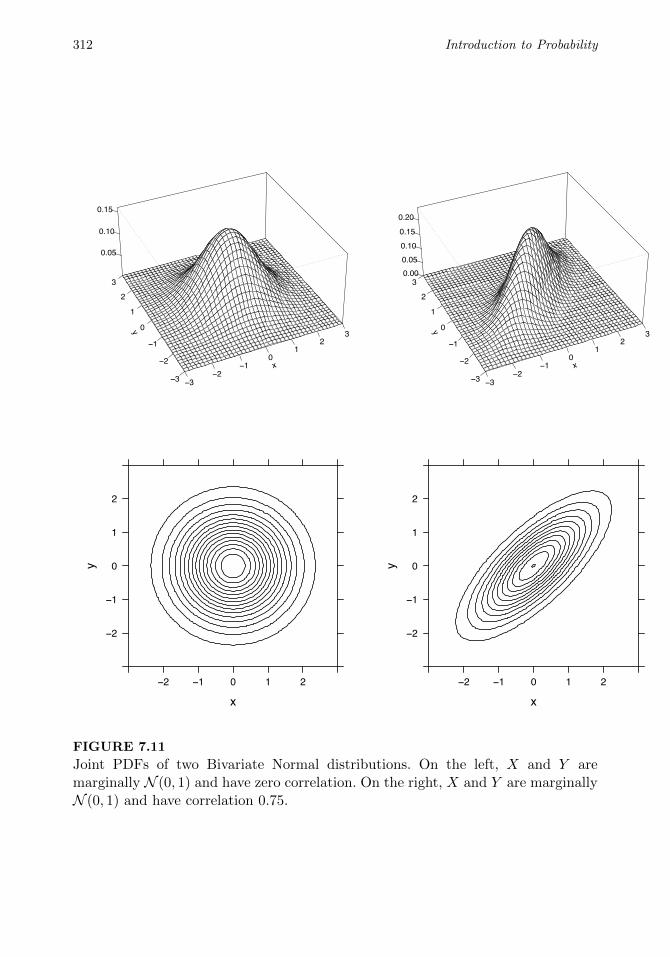
312 Introduction to Probability
x
−3−2
−10
12
3y
−3
−2
−1
0
1
2
3
0.05
0.10
0.15
x
−3−2
−10
12
3y
−3
−2
−1
0
1
2
30.000.050.100.15
0.20
x
y
−2
−1
0
1
2
−2 −1 0 1 2
x
y
−2
−1
0
1
2
−2 −1 0 1 2
FIGURE 7.11
Joint PDFs of two Bivariate Normal distributions. On the left, X and Y aremarginally N (0, 1) and have zero correlation. On the right, X and Y are marginallyN (0, 1) and have correlation 0.75.

Joint distributions 313
For a Multivariate Normal random vector, the joint MGF is particularly nice becausethe term in the exponent, t
1
X1
+ · · · + tkXk, is a Normal r.v. by definition. Thismeans we can use what we know about the univariate Normal MGF to find theMultivariate Normal joint MGF! Recall that for any Normal r.v. W ,
E(eW ) = eE(W )+
1
2
Var(W ).
Therefore the joint MGF of a Multivariate Normal (X1
, . . . , Xk) is
E(et1X1
+···+tk
Xk) = exp
✓t1
E(X1
) + · · ·+ tkE(Xk) +1
2Var(t
1
X1
+ · · ·+ tkXk)
◆.
The variance term can be expanded using properties of covariance.
We know that in general, independence is a stronger condition than zero correlation;r.v.s can be uncorrelated but not independent. A special property of the MultivariateNormal distribution is that for r.v.s whose joint distribution is MVN, independenceand zero correlation are equivalent conditions.
Theorem 7.5.7. Within an MVN random vector, uncorrelated implies indepen-dent. That is, if X ⇠ MVN can be written as X = (X
1
,X2
), where X1
and X2
aresubvectors, and every component of X
1
is uncorrelated with every component ofX
2
, then X1
and X2
are independent.1
In particular, if (X,Y ) is Bivariate Normal and Corr(X,Y ) = 0, then X and Y areindependent.
Proof. We will prove this theorem in the case of a Bivariate Normal; the proof inhigher dimensions is analogous. Let (X,Y ) be Bivariate Normal with E(X) = µ
1
,E(Y ) = µ
2
, Var(X) = �21
, Var(Y ) = �22
, and Corr(X,Y ) = ⇢. The joint MGF is
MX,Y (s, t) = E(esX+tY ) = exp
✓sµ
1
+ tµ2
+1
2Var(sX + tY )
◆
= exp
✓sµ
1
+ tµ2
+1
2(s2�2
1
+ t2�22
+ 2st�1
�2
⇢)
◆.
If ⇢ = 0, the joint MGF reduces to
MX,Y (s, t) = exp
✓sµ
1
+ tµ2
+1
2(s2�2
1
+ t2�22
)
◆.
But this is also the joint MGF of (Z,W ) where Z ⇠ N (µ1
,�21
) and W ⇠ N (µ2
,�22
)and Z is independent of W . Since the joint MGF determines the joint distribution,it must be that (X,Y ) has the same joint distribution as (Z,W ). Therefore X andY are independent. ⌅
1Independence of random vectors is defined analogously to independence of random variables.In particular, if Xi has joint PDF fX
i
, then it says that fX(x1
,x2
) = fX1
(x1
)fX2
(x2
) for all x1
,x2
.

314 Introduction to Probability
This theorem does not apply to Example 7.5.2. In that example, as you can verify,X and Y are uncorrelated and not independent, but this does not contradict thetheorem because (X,Y ) is not BVN. The next two examples show situations wherethe theorem does apply.
Example 7.5.8 (Independence of sum and di↵erence). Let X,Yi.i.d.⇠ N (0, 1). Find
the joint distribution of (X + Y,X � Y ).
Solution:
Since (X + Y,X � Y ) is Bivariate Normal and
Cov(X + Y,X � Y ) = Var(X)� Cov(X,Y ) + Cov(Y,X)�Var(Y ) = 0,
X + Y is independent of X � Y . Furthermore, they are i.i.d. N (0, 2). By the samemethod, we have that if X ⇠ N (µ
1
,�2) and Y ⇠ N (µ2
,�2) are independent (withthe same variance), then X + Y is independent of X � Y .
It can be shown that the independence of the sum and di↵erence is a unique char-acteristic of the Normal! That is, if X and Y are i.i.d. and X +Y is independent ofX � Y , then X and Y must have Normal distributions.
In Exercise 71, you’ll extend this example to the case where X and Y are BivariateNormal with general correlation ⇢. ⇤Example 7.5.9 (Independence of sample mean and sample variance). LetX
1
, . . . , Xn be i.i.d. N (µ,�2), with n � 2. Define
Xn =1
n(X
1
+ · · ·+Xn),
S2
n =1
n� 1
nX
j=1
(Xj � Xn)2.
As shown in Chapter 6, the sample mean Xn has expectation µ (the true mean)and the sample variance S2
n has expectation �2 (the true variance). Show that Xn
and S2
n are independent by applying MVN ideas and results to the vector (Xn, X1
�Xn, . . . , Xn � Xn).
Solution:
The vector (Xn, X1
� Xn, . . . , Xn � Xn) is MVN since any linear combination ofits components can be written as a linear combination of X
1
, . . . , Xn. Furthermore,E(Xj � Xn) = 0 by linearity. Now we compute the covariance of Xn with Xj � Xn:
Cov(Xn, Xj � Xn) = Cov(Xn, Xj)� Cov(Xn, Xn).
For Cov(Xn, Xj), we can expand out Xn, and most of the terms cancel due toindependence:
Cov(Xn, Xj) = Cov
✓1
nX
1
+ · · ·+ 1
nXn, Xj
◆= Cov
✓1
nXj , Xj
◆=
1
nVar(Xj) =
�2
n.

Joint distributions 315
For Cov(Xn, Xn), we use properties of variance:
Cov(Xn, Xn) = Var(Xn) =1
n2
(Var(X1
) + · · ·+Var(Xn)) =�2
n.
Therefore Cov(Xn, Xj � Xn) = 0, which means Xn is uncorrelated with every com-ponent of (X
1
�Xn, . . . , Xn�Xn). Since uncorrelated implies independent within anMVN vector, we have that Xn is independent of the vector (X
1
�Xn, . . . , Xn�Xn).But S2
n is a function of the vector (X1
�Xn, . . . , Xn�Xn), so Xn is also independentof S2
n.
It can be shown that the independence of the sample mean and variance is anotherunique characteristic of the Normal! If the Xj followed any other distribution, thenXn and S2
n would be dependent. ⇤Example 7.5.10 (Bivariate Normal generation). Suppose that we have access toi.i.d. r.v.s X,Y ⇠ N (0, 1), but want to generate a Bivariate Normal (Z,W ) withCorr(Z,W ) = ⇢ and Z,W marginally N (0, 1), for the purpose of running a simula-tion. How can we construct Z and W from linear combinations of X and Y ?
Solution:
By definition of Multivariate Normal, any (Z,W ) of the form
Z = aX + bY
W = cX + dY
will be Bivariate Normal. So let’s try to find suitable a, b, c, d. The means are already0. Setting the variances equal to 1 gives
a2 + b2 = 1, c2 + d2 = 1.
Setting the covariance of Z and W equal to ⇢ gives
ac+ bd = ⇢.
There are more unknowns than equations here, and we just need one solution. Tosimplify, let’s look for a solution with b = 0. Then a2 = 1, so let’s take a = 1. Nowac+ bd = ⇢ reduces to c = ⇢, and then we can use c2 + d2 = 1 to find a suitable d.Putting everything together, we can generate (Z,W ) as
Z = X
W = ⇢X +p
1� ⇢2Y.
Note that in the extreme case ⇢ = 1 (known as perfect positive correlation) this saysto let W = Z ⇠ N (0, 1), in the extreme case ⇢ = �1 (known as perfect negativecorrelation) it says to let W = �Z with Z ⇠ N (0, 1), and in the simple case ⇢ = 0it says to just let (Z,W ) = (X,Y ). ⇤

316 Introduction to Probability
7.6 Recap
Joint distributions allow us to describe the behavior of multiple random variablesthat arise from the same experiment. Important functions associated with a jointdistribution are the joint CDF, joint PMF/PDF, marginal PMF/PDF, and condi-tional PMF/PDF. The table below summarizes these definitions for two discreter.v.s and two continuous r.v.s. Joint distributions can also be a hybrid of discreteand continuous, in which case we mix and match PMFs and PDFs.
Two discrete r.v.s Two continuous r.v.s
Joint CDF FX,Y (x, y) = P (X x, Y y) FX,Y (x, y) = P (X x, Y y)
JointPMF/PDF
P (X = x, Y = y)
• Joint PMF is nonnegative and sums to 1:P
x
Py P (X = x, Y = y) = 1.
fX,Y (x, y) = @2
@x@yFX,Y (x, y)
• Joint PDF is nonnegative and integrates to 1:R1�1
R1�1 fX,Y (x, y)dxdy = 1.
• To get probability, integrate joint PDF over regionof interest.
MarginalPMF/PDF
P (X = x) =X
y
P (X = x, Y = y)
=X
y
P (X = x|Y = y)P (Y = y)
fX(x) =
Z 1
�1fX,Y (x, y)dy
=
Z 1
�1fX|Y (x|y)fY (y)dy
ConditionalPMF/PDF
P (Y = y|X = x) =P (X = x, Y = y)
P (X = x)
=P (X = x|Y = y)P (Y = y)
P (X = x)
fY |X(y|x) = fX,Y (x, y)fX(x)
=fX|Y (x|y)fY (y)
fX(x)
Independence P (X x, Y y) = P (X x)P (Y y)P (X = x, Y = y) = P (X = x)P (Y = y)
for all x and y.
P (Y = y|X = x) = P (Y = y)for all x and y, P (X = x) > 0.
P (X x, Y y) = P (X x)P (Y y)fX,Y (x, y) = fX(x)fY (y)
for all x and y.
fY |X(y|x) = fY (y)for all x and y, fX(x) > 0.
LOTUS E(g(X,Y )) =X
x
X
y
g(x, y)P (X = x, Y = y) E(g(X,Y )) =
Z 1
�1
Z 1
�1g(x, y)fX,Y (x, y)dxdy

Joint distributions 317
Covariance is a single-number summary of the tendency of two r.v.s to move in thesame direction. If two r.v.s are independent, then they are uncorrelated, but theconverse does not hold. Correlation is a unitless, standardized version of covariancethat is always between �1 and 1.
Two important named multivariate distributions are the Multinomial and Multi-variate Normal. The Multinomial distribution is a generalization of the Binomial;a Multk(n,p) random vector counts the number of objects, out of n, that fall intoeach of k categories, where p is the vector of probabilities for the k categories.
The Multivariate Normal distribution is a generalization of the Normal; a randomvector is defined to be MVN if any linear combination of its components has aNormal distribution. A key property of the MVN distribution is that within anMVN random vector, uncorrelated implies independent.
x
−3−2
−10
12
3y
−3
−2
−1
0
1
2
3
0.00
0.05
0.10
0.15
0.20
joint CDF F(x,y)joint PMF P(X = x,Y = y)
joint PDF f(x,y)joint MGF M(s,t)
(X,Y) P(X ≤ x, Y ≤ y) = F(x,y)P(X + Y < 3)
function of random vector
joint distributions random vectors events numbers
X ≤ x, Y ≤ yX + Y < 3
generate
E(X), Var(X), P(X ≤ x)E(Y), Var(Y), P(Y ≤ y)(marginal quantities)
X + YXY
g(X,Y)
2D LOTUS E(X + Y) = E(X) + E(Y)E(XY) = Cov(X,Y) + E(X)E(Y)
E(g(X,Y))
Cov(X,Y), Corr(X,Y)(joint quantities)
sum joint PMF or integrate joint PDF
over all y to getmarginal dist. of X
P(Y = y | X = x) = P(X = x, Y = y) / P(X = x)E(Y | X = x)
(quantities based on the conditional distribution of Y | X = x)
What can happen?
CDF FPMF story
name, parameters
XP(X ≤ x) = F(x)
P(X = x)
func
tion o
f r.v.
X ≤ xX = x
generate
E(X), Var(X), SD(X)
X, X2, X3, …g(X)
LOTUS E(X), E(X2), E(X3), …E(g(X))
distributions random variables numbersevents
What can happen?
P
P
FIGURE 7.12
Fundamental objects of probability for multivariate distributions. A joint distribu-tion is determined by a joint CDF, joint PMF/PDF, or joint MGF. A random vector(X,Y ) gives rise to many useful joint, marginal, and conditional quantities. Using2D LOTUS, we can find the expected value of a function of X and Y . Summing thejoint PMF or integrating the joint PDF over all y gives the marginal distributionof X, bringing us back to the case of a one-dimensional distribution.
Figure 7.12 extends our diagram of the fundamental objects of probability to the

318 Introduction to Probability
multivariate setting (taken as bivariate to simplify notation). A joint distributioncan be used to generate random vectors (X,Y ). Various joint, marginal, and con-ditional quantities can then be studied. Summing the joint PMF or integrating thejoint PDF over all y gives the marginal distribution of X, bringing us back to theone-dimensional realm.
7.7 R
Multinomial
The functions for the Multinomial distribution are dmultinom (which is the jointPMF of the Multinomial distribution) and rmultinom (which generates realizationsof Multinomial random vectors). The joint CDF of the Multinomial is a pain towork with, so it is not built into R.
To use dmultinom, we have to input the value at which to evaluate the joint PMF,as well as the parameters of the distribution. For example,
x <- c(2,0,3)
n <- 5
p <- c(1/3,1/3,1/3)
dmultinom(x,n,p)
returns the probability P (X1
= 2, X2
= 0, X3
= 3), where
X = (X1
, X2
, X3
) ⇠ Mult3
(5, (1/3, 1/3, 1/3)).
Of course, n has to equal sum(x); if we attempted to do dmultinom(x,7,p), Rwould report an error.
For rmultinom, the first input is the number of Multinomial random vectors togenerate, and the other inputs are the same. When we typed rmultinom(10,n,p)
with n and p as above, R gave us the following matrix:
0 2 1 3 2 3 1 2 3 4
2 2 2 2 3 0 1 2 0 0
3 1 2 0 0 2 3 1 2 1
Each column of the matrix corresponds to a draw from the Mult3
(5, (1/3, 1/3, 1/3))distribution. In particular, the sum of each column is 5.
Multivariate Normal
Functions for the Multivariate Normal distribution are located in the packagemvtnorm. Online resources can teach you how to install packages in R for your sys-

Joint distributions 319
tem, but for many systems an easy way is to use the install.packages command,e.g., by typing install.packages("mvtnorm") to install the mvtnorm package. Af-ter installing, load the package with library(mvtnorm). Then dmvnorm can be usedfor calculating the joint PDF, and rmvnorm can be used for generating random vec-tors. For example, suppose that we want to generate 1000 independent BivariateNormal pairs (Z,W ), with correlation ⇢ = 0.7 and N (0, 1) marginals. To do this,we can enter the following:
meanvector <- c(0,0)
rho <- 0.7
covmatrix <- matrix(c(1,rho,rho,1), nrow = 2, ncol = 2)
r <- rmvnorm(n = 10^3, mean = meanvector, sigma = covmatrix)
The covariance matrix here is 0
B@1 ⇢
⇢ 1
1
CA
because
• Cov(Z,Z) = Var(Z) = 1 (this is the upper left entry)
• Cov(W,W ) = Var(W ) = 1 (this is the lower right entry)
• Cov(Z,W ) = Corr(Z,W )SD(Z)SD(W ) = ⇢ (this is the other two entries).
Now r is a 1000 ⇥ 2 matrix, with each row a BVN random vector. To see theseas points in the plane, we can use plot(r) to make a scatter plot, from which thestrong positive correlation should be clear. To estimate the covariance of Z and W ,we can use cov(r), which the true covariance matrix.
Example 7.5.10 gives another approach to the BVN generation problem:
rho <- 0.7
tau <- sqrt(1-rho^2)
x <- rnorm(10^3)
y <- rnorm(10^3)
z <- x
w <- rho*x + tau*y
This gives the Z-coordinates in a vector z and the W -coordinates in a vector w.If we want to put them into one 1000 ⇥ 2 matrix as we had above, we can typecbind(z,w) to bind the vectors together as columns.
Cauchy
We can work with the Cauchy distribution introduced in Example 7.1.24 usingthe three functions dcauchy, pcauchy, and rcauchy. Only one input is needed; forexample, dcauchy(0) is the Cauchy PDF evaluated at 0.

320 Introduction to Probability
For an amusing demonstration of the very heavy tails of the Cauchy distribution,try creating a histogram of 1000 simulated values of the Cauchy distribution:
hist(rcauchy(1000))
Due to extreme values in the tails of the distribution, this histogram looks nothinglike the PDF of the distribution from which it was generated.
7.8 Exercises
Joint, marginal, and conditional distributions
1. Alice and Bob arrange to meet for lunch on a certain day at noon. However, neither isknown for punctuality. They both arrive independently at uniformly distributed timesbetween noon and 1 pm on that day. Each is willing to wait up to 15 minutes for theother to show up. What is the probability they will meet for lunch that day?
2. Alice, Bob, and Carl arrange to meet for lunch on a certain day. They arrive indepen-dently at uniformly distributed times between 1 pm and 1:30 pm on that day.
(a) What is the probability that Carl arrives first?
For the rest of this problem, assume that Carl arrives first at 1:10 pm, and condition onthis fact.
(b) What is the probability that Carl will have to wait more than 10 minutes for one ofthe others to show up? (So consider Carl’s waiting time until at least one of the othershas arrived.)
(c) What is the probability that Carl will have to wait more than 10 minutes for bothof the others to show up? (So consider Carl’s waiting time until both of the others hasarrived.)
(d) What is the probability that the person who arrives second will have to wait morethan 5 minutes for the third person to show up?
3. One of two doctors, Dr. Hibbert and Dr. Nick, is called upon to perform a series ofn surgeries. Let H be the indicator r.v. for Dr. Hibbert performing the surgeries, andsuppose that E(H) = p. Given that Dr. Hibbert is performing the surgeries, each surgeryis successful with probability a, independently. Given that Dr. Nick is performing thesurgeries, each surgery is successful with probability b, independently. Let X be thenumber of successful surgeries.
(a) Find the joint PMF of H and X.
(b) Find the marginal PMF of X.
(c) Find the conditional PMF of H given X = k.
4. A fair coin is flipped twice. Let X be the number of Heads in the two tosses, and Y bethe indicator r.v for the tosses landing the same way.
(a) Find the joint PMF of X and Y .
(b) Find the marginal PMFs of X and Y .
(c) Are X and Y independent?
(d) Find the conditional PMFs of Y given X = x and of X given Y = y.

Joint distributions 321
5. A fair die is rolled, and then a coin with probability p of Heads is flipped as many timesas the die roll says, e.g., if the result of the die roll is a 3, then the coin is flipped 3times. Let X be the result of the die roll and Y be the number of times the coin landsHeads.
(a) Find the joint PMF of X and Y . Are they independent?
(b) Find the marginal PMFs of X and Y .
(c) Find the conditional PMFs of Y given X = x and of Y given X = x.
6. A committee of size k is chosen from a group of n women and m men. All possiblecommittees of size k are equally likely. Let X and Y be the numbers of women and menon the committee, respectively.
(a) Find the joint PMF of X and Y . Be sure to specify the support.
(b) Find the marginal PMF of X in two di↵erent ways: by doing a computation usingthe joint PMF, and using a story.
(c) Find the conditional PMF of Y given that X = x.
7. A stick of length L (a positive constant) is broken at a uniformly random point X.Given that X = x, another breakpoint Y is chosen uniformly on the interval [0, x].
(a) Find the joint PDF of X and Y . Be sure to specify the support.
(b) We already know that the marginal distribution of X is Unif(0, L). Check thatmarginalizing out Y from the joint PDF agrees that this is the marginal distribution ofX.
(c) We already know that the conditional distribution of Y given X = x is Unif(0, x).Check that using the definition of conditional PDFs (in terms of joint and marginalPDFs) agrees that this is the conditional distribution of Y given X = x.
(d) Find the marginal PDF of Y .
(e) Find the conditional PDF of X given Y = y.
8. (a) Five cards are randomly chosen from a standard deck, one at a time with replacement.Let X,Y, Z be the numbers of chosen queens, kings, and other cards. Find the joint PMFof X,Y, Z.
(b) Find the joint PMF of X and Y .
Hint: In summing the joint PMF of X,Y, Z over the possible values of Z, note that mostterms are 0 because of the constraint that the number of chosen cards is five.
(c) Now assume instead that the sampling is without replacement (all 5-card hands areequally likely). Find the joint PMF of X,Y, Z.
Hint: Use the naive definition of probability.
9. Let X and Y be i.i.d. Geom(p), and N = X + Y .
(a) Find the joint PMF of X,Y,N .
(b) Find the joint PMF of X and N .
(c) Find the conditional PMF of X given N = n, and give a simple description in wordsof what the result says.

322 Introduction to Probability
10. Let X and Y be i.i.d. Expo(�), and T = X + Y .
(a) Find the conditional CDF of T given X = x. Be sure to specify where it is zero.
(b) Find the conditional PDF fT |X(t|x), and verify that it is a valid PDF.
(c) Find the conditional PDF fX|T (x|t), and verify that it is a valid PDF.
Hint: This can be done using Bayes’ rule without having to know the marginal PDF ofT , by recognizing what the conditional PDF is up to a normalizing constant—then thenormalizing constant must be whatever is needed to make the conditional PDF valid.
(d) In Example 8.2.4, we will show that the marginal PDF of T is fT (t) = �2te��t, fort > 0. Give a short alternative proof of this fact, based on the previous parts and Bayes’rule.
11. Let X,Y, Z be r.v.s such that X ⇠ N (0, 1) and conditional on X = x, Y and Z arei.i.d. N (x, 1).
(a) Find the joint PDF of X,Y, Z.
(b) By definition, Y and Z are conditionally independent given X. Discuss intuitivelywhether or not Y and Z are also unconditionally independent.
(c) Find the joint PDF of Y and Z. You can leave your answer as an integral, thoughthe integral can be done with some algebra (such as completing the square) and factsabout the Normal distribution.
12. Let X ⇠ Expo(�), and let c be a positive constant.
(a) If you remember the memoryless property, you already know that the conditionaldistribution of X given X > c is the same as the distribution of c+X (think of waitingc minutes for a “success” and then having a fresh Expo(�) additional waiting time).Derive this in another way, by finding the conditional CDF of X given X > c and theconditional PDF of X given X > c.
(b) Find the conditional CDF of X given X < c and the conditional PDF of X givenX < c.
13. Let X and Y be i.i.d. Expo(�). Find the conditional distribution of X given X < Y intwo di↵erent ways:
(a) by using calculus to find the conditional PDF.
(b) without using calculus, by arguing that the conditional distribution of X givenX < Y is the same distribution as the unconditional distribution of min(X,Y ), andthen applying an earlier result about the minimum of independent Exponentials.
14. s� (a) A stick is broken into three pieces by picking two points independently anduniformly along the stick, and breaking the stick at those two points. What is theprobability that the three pieces can be assembled into a triangle?
Hint: A triangle can be formed from 3 line segments of lengths a, b, c if and only ifa, b, c 2 (0, 1/2). The probability can be interpreted geometrically as proportional toan area in the plane, avoiding all calculus, but make sure for that approach that thedistribution of the random point in the plane is Uniform over some region.
(b) Three legs are positioned uniformly and independently on the perimeter of a roundtable. What is the probability that the table will stand?
15. Let X and Y be continuous r.v.s., with joint CDF F (x, y). Show that the probabilitythat (X,Y ) falls into the rectangle [a
1
, a2
]⇥ [b1
, b2
] is
F (a2
, b2
)� F (a1
, b2
) + F (a1
, b1
)� F (a2
, b1
).
Joint distributions 323
16. Let X and Y have joint PDF
fX,Y (x, y) = x+ y, for 0 < x < 1 and 0 < y < 1.
(a) Check that this is a valid joint PDF.
(b) Are X and Y independent?
(c) Find the marginal PDFs of X and Y .
(d) Find the conditional PDF of Y given X = x.
17. Let X and Y have joint PDF
fX,Y (x, y) = cxy, for 0 < x < y < 1.
(a) Find c to make this a valid joint PDF.
(b) Are X and Y independent?
(c) Find the marginal PDFs of X and Y .
(d) Find the conditional PDF of Y given X = x.
18. s� Let (X,Y ) be a uniformly random point in the triangle in the plane with vertices(0, 0), (0, 1), (1, 0). Find the joint PDF of X and Y , the marginal PDF of X, and theconditional PDF of X given Y .
19. s� A random point (X,Y, Z) is chosen uniformly in the ball B = {(x, y, z) : x2+y2+z2 1}.
(a) Find the joint PDF of X,Y, Z.
(b) Find the joint PDF of X,Y .
(c) Find an expression for the marginal PDF of X, as an integral.
20. s� Let U1
, U2
, U3
be i.i.d. Unif(0, 1), and let L = min(U1
, U2
, U3
),M = max(U1
, U2
, U3
).
(a) Find the marginal CDF and marginal PDF of M, and the joint CDF and joint PDFof L,M .
Hint: For the latter, start by considering P (L � l,M m).
(b) Find the conditional PDF of M given L.
21. Find the probability that the quadratic polynomial Ax2+Bx+1, where the coe�cientsA and B are determined by drawing i.i.d. Unif(0, 1) random variables, has at least onereal root.
Hint: By the quadratic formula, the polynomial ax2 + bx+ c has a real root if and onlyif b2 � 4ac � 0.
22. Let X and Y each have support (0,1) marginally, and suppose that the joint PDFfX,Y of X and Y is positive for 0 < x < y and 0 otherwise.
(a) What is the support of the conditional PDF of Y given X = x?
(b) Show that X and Y can’t be independent.
23. The volume of a region in n-dimensional Euclidean space Rn is the integral of 1 overthat region. The unit ball in Rn is {(x
1
, . . . , xn) : x2
1
+ · · ·+ x2
n 1}, the ball of radius1 centered at 0. As mentioned in Section A.7 of the math appendix, the volume of theunit ball in n dimensions is
vn =⇡n/2
�(n/2 + 1),

324 Introduction to Probability
where � is the gamma function, a very famous function which is defined by
�(a) =
Z 1
0
xae�x dx
x
for all a > 0, and which will play an important role in the next chapter. A few usefulfacts about the gamma function (which you can assume) are that �(a + 1) = a�(a)for any a > 0, and that �(1) = 1 and �( 1
2
) =p⇡. Using these facts, it follows that
�(n) = (n � 1)! for n a positive integer, and we can also find �(n + 1
2
) when n is anonnegative integer. For practice, please verify that v
2
= ⇡ (the area of the unit disk in2 dimensions) and v
3
= 4
3
⇡ (the volume of the unit ball in 3 dimensions).
Let U1
, U2
, . . . , Un ⇠ Unif(�1, 1) be i.i.d.
(a) Find the probability that (U1
, U2
, . . . , Un) is in the unit ball in Rn.
(b) Evaluate the result from (a) numerically for n = 1, 2, . . . , 10, and plot the results(using a computer unless you are extremely good at making hand-drawn graphs). Thefacts above about the gamma function are su�cient so that you can do this withoutdoing any integrals, but you can also use the command gamma in R to compute thegamma function.
(c) Let c be a constant with 0 < c < 1, and let Xn count how many of the Uj satisfy|Uj | > c. What is the distribution of Xn?
(d) For c = 1/p2, use the result of Part (c) to give a simple, short derivation of what
happens to the probability from (a) as n ! 1.
24. s� Two students, A and B, are working independently on homework (not necessarily forthe same class). Student A takes Y
1
⇠ Expo(�1
) hours to finish his or her homework,while B takes Y
2
⇠ Expo(�2
) hours.
(a) Find the CDF and PDF of Y1
/Y2
, the ratio of their problem-solving times.
(b) Find the probability that A finishes his or her homework before B does.
25. Two companies, Company 1 and Company 2, have just been founded. Stock marketcrashes occur according to a Poisson process with rate �
0
. Such a crash would put bothcompanies out of business. For j 2 {1, 2}, there may be an adverse event “of type j,”which puts Company j out of business (if it is not already out of business) but does nota↵ect the other company; such events occur according to a Poisson process with rate �j .If there has not been a stock market crash or an adverse event of type j, then companyj remains in business. The three Poisson processes are independent of each other. LetX
1
and X2
be how long Company 1 and Company 2 stay in business, respectively.
(a) Find the marginal distributions of X1
and X2
.
(b) Find P (X1
> x1
, X2
> x2
), and use this to find the joint CDF of X1
and X2
.
26. s� The bus company from Blissville decides to start service in Blotchville, sensing apromising business opportunity. Meanwhile, Fred has moved back to Blotchville. Nowwhen Fred arrives at the bus stop, either of two independent bus lines may come by(both of which take him home). The Blissville company’s bus arrival times are exactly10 minutes apart, whereas the time from one Blotchville company bus to the next isExpo( 1
10
). Fred arrives at a uniformly random time on a certain day.
(a) What is the probability that the Blotchville company bus arrives first?
Hint: One good way is to use the continuous law of total probability.
(b) What is the CDF of Fred’s waiting time for a bus?
Joint distributions 325
27. A longevity study is being conducted on n married hobbit couples. Let p be the proba-bility that an individual hobbit lives at least until his or her eleventy-first birthday, andassume that the lifespans of di↵erent hobbits are independent. Let N
0
, N1
, N2
be thenumber of couples in which neither hobbit reaches age eleventy-one, one hobbit doesbut not the other, and both hobbits reach eleventy-one, respectively.
(a) Find the joint PMF of N0
, N1
, N2
.
(b) Using (a) and the definition of conditional probability, find the conditional PMF ofN
2
given this information, up to a normalizing constant (that is, you do not need tofind the normalizing constant in this part, but just to give a simplified expression thatis proportional to the conditional PMF). For simplicity, you can and should ignore mul-tiplicative constants in this part; this includes multiplicative factors that are functionsof h, since h is now being treated as a known constant.
(c) Now obtain the conditional PMF of N2
using a direct counting argument, nowincluding any needed normalizing constants so that you are providing a valid conditionalPMF.
(d) Discuss intuitively whether or not p should appear in the answer to (c).
(e) What is the conditional expectation of N2
, given the above information (simplifyfully)? This can be done without doing any messy sums, and without having done (b)or (c).
28. There are n stores in a shopping center, labeled from 1 to n. Let Xi be the numberof customers who visit store i in a particular month, and suppose that X
1
, X2
, . . . , Xn
are i.i.d. with PMF p(x) = P (Xi = x). Let I ⇠ DUnif(1, 2, . . . , n) be the label of arandomly chosen store, so XI is the number of customers at a randomly chosen store.
(a) For i 6= j, find P (Xi = Xj) in terms of a sum involving the PMF p(x).
(b) Find the joint PMF of I and XI . Are they independent?
(c) Does XI , the number of customers for a random store, have the same marginaldistribution as X
1
, the number of customers for store 1?
(d) Let J ⇠ DUnif(1, 2, . . . , n) also be the label of a randomly chosen store, with I andJ independent. Find P (XI = XJ) in terms of a sum involving the PMF p(x). How doesP (XI = XJ) compare to P (Xi = Xj) for fixed i, j with i 6= j?
29. Let X and Y be i.i.d. Geom(p), L = min(X,Y ), and M = max(X,Y ).
(a) Find the joint PMF of L and M . Are they independent?
(b) Find the marginal distribution of L in two ways: using the joint PMF, and using astory.
(c) Find EM .
Hint: A quick way is to use (b) and the fact that L+M = X + Y .
(d) Find the joint PMF of L and M � L. Are they independent?
30. Let X,Y have the joint CDF
F (x, y) = 1� e�x � e�y + e�(x+y+✓xy),
for x > 0, y > 0 (and F (x, y) = 0 otherwise), where the parameter ✓ is a constant in[0, 1].
(a) Find the joint PDF of X,Y . For which values of ✓ (if any) are they independent?
(b) Explain why we require ✓ to be in [0, 1].

326 Introduction to Probability
(c) Find the marginal PDFs of X and Y by working directly from the joint PDF from(a). When integrating, do not use integration by parts or computer assistance; rather,pattern match to facts we know about moments of famous distributions.
(d) Find the marginal CDFs of X and Y by working directly from the joint CDF.
2D LOTUS
31. s� Let X and Y be i.i.d. Unif(0, 1). Find the standard deviation of the distance betweenX and Y .
32. s� Let X,Y be i.i.d. Expo(�). Find E|X�Y | in two di↵erent ways: (a) using 2D LOTUSand (b) using the memoryless property without any calculus.
33. Alice walks into a post o�ce with 2 clerks. Both clerks are in the midst of servingcustomers, but Alice is next in line. The clerk on the left takes an Expo(�
1
) time toserve a customer, and the clerk on the right takes an Expo(�
2
) time to serve a customer.Let T be the amount of time Alice has to wait until it is her turn.
(a) Write down expressions for the mean and variance of T , in terms of double integrals(which you do not need to evaluate).
(b) Find the distribution, mean, and variance of T , without using calculus.
34. Let (X,Y ) be a uniformly random point in the triangle in the plane with vertices(0, 0), (0, 1), (1, 0). Find Cov(X,Y ). (Exercise 18 is about joint, marginal, and condi-tional PDFs in this setting.)
35. A random point is chosen uniformly in the unit disk {(x, y) : x2 + y2 1}. Let R be itsdistance from the origin.
(a) Find E(R) using 2D LOTUS.
Hint: To do the integral, convert to polar coordinates (see the math appendix).
(b) Find the CDFs of R2 and of R without using calculus, using the fact that for aUniform distribution on a region, probability within that region is proportional to area.Then get the PDFs of R2 and of R, and find E(R) in two more ways: using the definitionof expectation, and using a 1D LOTUS by thinking of R as a function of R2.
36. Let X and Y be discrete r.v.s.
(a) Use 2D LOTUS (without assuming linearity) to show that E(X+Y ) = E(X)+E(Y ).
(b) Now suppose that X and Y are independent. Use 2D LOTUS to show that E(XY ) =E(X)E(Y ).
37. Let X and Y be i.i.d. continuous random variables with PDF f , mean µ, and variance�2. We know that the expected squared distance of X from its mean is �2, and likewisefor Y ; this problem is about the expected squared distance of X from Y .
(a) Use 2D LOTUS to express E(X � Y )2 as a double integral.
(b) By expanding (x� y)2 = x2 � 2xy+ y2 and evaluating the double integral from (a),show that
E(X � Y )2 = 2�2.
(c) Give an alternative proof of the result from (b), based on the trick of adding andsubtracting µ:
(X � Y )2 = (X � µ+ µ� Y )2 = (X � µ)2 � 2(X � µ)(Y � µ) + (Y � µ)2.

Joint distributions 327
Covariance
38. s� Let X and Y be r.v.s. Is it correct to say “max(X,Y ) + min(X,Y ) = X + Y ”? Is itcorrect to say “Cov(max(X,Y ),min(X,Y )) = Cov(X,Y ) since either the max is X andthe min is Y or vice versa, and covariance is symmetric”? Explain.
39. s� Two fair six-sided dice are rolled (one green and one orange), with outcomes X andY respectively for the green and the orange.
(a) Compute the covariance of X + Y and X � Y .
(b) Are X + Y and X � Y independent?
40. Let X and Y be i.i.d. Unif(0, 1).
(a) Compute the covariance of X + Y and X � Y .
(b) Are X + Y and X � Y independent?
41. s� Let X and Y be standardized r.v.s (i.e., marginally they each have mean 0 andvariance 1) with correlation ⇢ 2 (�1, 1). Find a, b, c, d (in terms of ⇢) such that Z =aX + bY and W = cX + dY are uncorrelated but still standardized.
42. s� Let X be the number of distinct birthdays in a group of 110 people (i.e., the numberof days in a year such that at least one person in the group has that birthday). Underthe usual assumptions (no February 29, all the other 365 days of the year are equallylikely, and the day when one person is born is independent of the days when the otherpeople are born), find the mean and variance of X.
43. (a) Let X and Y be Bernoulli r.v.s, possibly with di↵erent parameters. Show that if Xand Y are uncorrelated, then they are independent.
(b) Give an example of three Bernoulli r.v.s such that each pair of them is uncorrelated,yet the three r.v.s are dependent.
44. Find the variance of the number of toys needed until you have a complete set in Exam-ple 4.3.11 (the coupon collector problem).
45. A random triangle is formed in some way, such that the angles are identically distributed.What is the correlation between two of the angles (assuming that the variance of theangles is nonzero)?
46. Each of n � 2 people puts his or her name on a slip of paper (no two have the samename). The slips of paper are shu✏ed in a hat, and then each person draws one (uni-formly at random at each stage, without replacement). Find the standard deviation ofthe number of people who draw their own names.
47. s� Athletes compete one at a time at the high jump. Let Xj be how high the jthjumper jumped, with X
1
, X2
, . . . i.i.d. with a continuous distribution. We say that thejth jumper sets a record if Xj is greater than all of Xj�1
, . . . , X1
.
Find the variance of the number of records among the first n jumpers (as a sum). Whathappens to the variance as n ! 1?
48. s� A chicken lays a Pois(�) number N of eggs. Each egg hatches a chick with probabilityp, independently. Let X be the number which hatch, so X|N = n ⇠ Bin(n, p).
Find the correlation between N (the number of eggs) and X (the number of eggs whichhatch). Simplify; your final answer should work out to a simple function of p (the �should cancel out).
49. Let X1
, . . . , Xn be random variables such that Corr(Xi, Xj) = ⇢ for all i 6= j. Show that⇢ � � 1
n�1
. This is a bound on how negatively correlated a collection of r.v.s can all bewith each other.
Hint: Assume Var(Xi) = 1 for all i; this can be done without loss of generality, sincerescaling two r.v.s does not a↵ect the correlation between them. Then use the fact thatVar(X
1
+ · · ·+Xn) � 0.

328 Introduction to Probability
50. Let X and Y be independent r.v.s. Show that
Var(XY ) = Var(X)Var(Y ) + (EX)2Var(Y ) + (EY )2Var(X).
Hint: It is often useful when working with a second moment E(T 2) to write it as Var(T )+(ET )2.
51. Stat 110 shirts come in 3 sizes: small, medium, and large. There are n shirts of eachsize (where n � 2). There are 3n students. For each size, n of the students have thatsize as the best fit. This seems ideal. But suppose that instead of giving each studentthe right size shirt, each student is given a shirt completely randomly (all allocations ofthe shirts to the students, with one shirt per student, are equally likely). Let X be thenumber of students who get their right size shirt.
(a) Find E(X).
(b) Give each student an ID number from 1 to 3n, such that the right size shirt is smallfor students 1 through n, medium for students n+1 through 2n, and large for students2n + 1 through 3n. Let Aj be the event that student j gets their right size shirt. FindP (A
1
, A2
) and P (A1
, An+1
).
(c) Find Var(X).
52. s� A drunken man wanders around randomly in a large space. At each step, he movesone unit of distance North, South, East, or West, with equal probabilities. Choosecoordinates such that his initial position is (0, 0) and if he is at (x, y) at some time, thenone step later he is at (x, y+1), (x, y� 1), (x+1, y), or (x� 1, y). Let (Xn, Yn) and Rn
be his position and distance from the origin after n steps, respectively.
General hint: Note that Xn is a sum of r.v.s with possible values �1, 0, 1, and likewisefor Yn, but be careful throughout the problem about independence.
(a) Determine whether or not Xn is independent of Yn.
(b) Find Cov(Xn, Yn).
(c) Find E(R2
n).
53. s� A scientist makes two measurements, considered to be independent standard Normalr.v.s. Find the correlation between the larger and smaller of the values.
Hint: Note that max(x, y) + min(x, y) = x+ y and max(x, y)�min(x, y) = |x� y|.54. Let U ⇠ Unif(�1, 1) and V = 2|U |� 1.
(a) Find the distribution of V (give the PDF and, if it is a named distribution we havestudied, its name and parameters).
Hint: Find the support of V , and then find the CDF of V by reducing P (V v) toprobability calculations about U .
(b) Show that U and V are uncorrelated, but not independent. This is also anotherexample illustrating the fact that knowing the marginal distributions of two r.v.s doesnot determine the joint distribution.
55. s� Consider the following method for creating a bivariate Poisson (a joint distributionfor two r.v.s such that both marginals are Poissons). Let X = V +W,Y = V +Z whereV,W,Z are i.i.d. Pois(�) (the idea is to have something borrowed and something newbut not something old or something blue).
(a) Find Cov(X,Y ).
(b) Are X and Y independent? Are they conditionally independent given V ?
(c) Find the joint PMF of X,Y (as a sum).

Joint distributions 329
56. You are playing an exciting game of Battleship. Your opponent secretly positions shipson a 10 by 10 grid and you try to guess where the ships are. Each of your guesses is ahit if there is a ship there and a miss otherwise.
The game has just started and your opponent has 3 ships: a battleship (length 4), asubmarine (length 3), and a destroyer (length 2). (Usually there are 5 ships to start, butto simplify the calculations we are considering 3 here.) You are playing a variation inwhich you unleash a salvo, making 5 simultaneous guesses. Assume that your 5 guessesare a simple random sample drawn from the 100 grid positions.
Find the mean and variance of the number of distinct ships you will hit in your salvo.(Give exact answers in terms of binomial coe�cients or factorials, and also numericalvalues computed using a computer.)
Hint: First work in terms of the number of ships missed, expressing this as a sum ofindicator r.v.s. Then use the fundamental bridge and naive definition of probability,which can be applied since all sets of 5 grid positions are equally likely.
57. This problem explores a visual interpretation of covariance. Data are collected for n �2 individuals, where for each individual two variables are measured (e.g., height andweight). Assume independence across individuals (e.g., person 1’s variables gives noinformation about the other people), but not within individuals (e.g., a person’s heightand weight may be correlated).
Let (x1
, y1
), . . . , (xn, yn) be the n data points. The data are considered here as fixed,known numbers–they are the observed values after performing an experiment. Imagineplotting all the points (xi, yi) in the plane, and drawing the rectangle determined byeach pair of points. For example, the points (1, 3) and (4, 6) determine the rectanglewith vertices (1, 3), (1, 6), (4, 6), (4, 3).
The signed area contributed by (xi, yi) and (xj , yj) is the area of the rectangle theydetermine if the slope of the line between them is positive, and is the negative of thearea of the rectangle they determine if the slope of the line between them is negative.(Define the signed area to be 0 if xi = xj or yi = yj , since then the rectangle isdegenerate.) So the signed area is positive if a higher x value goes with a higher y valuefor the pair of points, and negative otherwise. Assume that the xi are all distinct andthe yi are all distinct.
(a) The sample covariance of the data is defined to be
r =1n
nX
i=1
(xi � x)(yi � y),
where
x =1n
nX
i=1
xi and y =1n
nX
i=1
yi
are the sample means. (There are di↵ering conventions about whether to divide byn� 1 or n in the definition of sample covariance, but that need not concern us for thisproblem.)
Let (X,Y ) be one of the (xi, yi) pairs, chosen uniformly at random. Determine preciselyhow Cov(X,Y ) is related to the sample covariance.
(b) Let (X,Y ) be as in (a), and (X, Y ) be an independent draw from the same distribu-tion. That is, (X,Y ) and (X, Y ) are randomly chosen from the n points, independently(so it is possible for the same point to be chosen twice).
Express the total signed area of the rectangles as a constant times E((X � X)(Y � Y )).Then show that the sample covariance of the data is a constant times the total signedarea of the rectangles.
Hint: Consider E((X�X)(Y �Y )) in two ways: as the average signed area of the random

330 Introduction to Probability
rectangle formed by (X,Y ) and (X, Y ), and using properties of expectation to relateit to Cov(X,Y ). For the former, consider the n2 possibilities for which point (X,Y ) isand which point (X, Y ); note that n such choices result in degenerate rectangles.
(c) Based on the interpretation from (b), give intuitive explanations of why for any r.v.sW
1
,W2
,W3
and constants a1
, a2
, covariance has the following properties:
(i) Cov(W1
,W2
) = Cov(W2
,W1
);
(ii) Cov(a1
W1
, a2
W2
) = a1
a2
Cov(W1
,W2
);
(iii) Cov(W1
+ a1
,W2
+ a2
) = Cov(W1
,W2
);
(iv) Cov(W1
,W2
+W3
) = Cov(W1
,W2
) + Cov(W1
,W3
).
58. A statistician is trying to estimate an unknown parameter ✓ based on some data. Shehas available two independent estimators ✓
1
and ✓2
(an estimator is a function of thedata, used to estimate a parameter). For example, ✓
1
could be the sample mean of asubset of the data and ✓
2
could be the sample mean of another subset of the data,disjoint from the subset used to calculate ✓
1
. Assume that both of these estimators areunbiased, i.e., E(✓j) = ✓.
Rather than having a bunch of separate estimators, the statistician wants one combinedestimator. It may not make sense to give equal weights to ✓
1
and ✓2
since one could bemuch more reliable than the other, so she decides to consider combined estimators ofthe form
✓ = w1
✓1
+ w2
✓2
,
a weighted combination of the two estimators. The weights w1
and w2
are nonnegativeand satisfy w
1
+ w2
= 1.
(a) Check that ✓ is also unbiased, i.e., E(✓) = ✓.
(b) Determine the optimal weights w1
, w2
, in terms of minimizing the mean squarederror E(✓�✓)2. Express your answer in terms of the variances of ✓
1
and ✓2
. The optimalweights are known as Fisher weights.
Hint: As discussed in Exercise 55 from Chapter 5, mean squared error is variance plussquared bias, so in this case the mean squared error of ✓ is Var(✓). Note that there isno need for multivariable calculus here, since w
2
= 1� w1
.
(c) Give a simple description of what the estimator found in (b) amounts to if the dataare i.i.d. random variables X
1
, . . . , Xn, Y1
, . . . , Ym, ✓1
is the sample mean of X1
, . . . , Xn,and ✓
2
is the sample mean of Y1
, . . . , Ym.
Chicken-egg
59. s� A Pois(�) number of people vote in a certain election. Each voter votes for candidateA with probability p and for candidate B with probability q = 1� p, independently ofall the other voters. Let V be the di↵erence in votes, defined as the number of votes forA minus the number for B.
(a) Find E(V ).
(b) Find Var(V ).
60. A traveler gets lost N ⇠ Pois(�) times on a long journey. When lost, the traveler askssomeone for directions with probability p. LetX be the number of times that the traveleris lost and asks for directions, and Y be the number of times that the traveler is lostand does not ask for directions.
(a) Find the joint PMF of N,X, Y . Are they independent?
(b) Find the joint PMF of N,X. Are they independent?
(c) Find the joint PMF of X,Y . Are they independent?
Joint distributions 331
61. The number of people who visit the Leftorium store in a day is Pois(100). Suppose that10% of customers are sinister (left-handed), and 90% are dexterous (right-handed). Halfof the sinister customers make purchases, but only a third of the dexterous customersmake purchases. The characteristics and behavior of people are independent, with prob-abilities as described in the previous two sentences. On a certain day, there are 42 peoplewho arrive at the store but leave without making a purchase. Given this information,what is the conditional PMF of the number of customers on that day who make apurchase?
62. A chicken lays n eggs. Each egg independently does or doesn’t hatch, with probability pof hatching. For each egg that hatches, the chick does or doesn’t survive (independentlyof the other eggs), with probability s of survival. Let N ⇠ Bin(n, p) be the number ofeggs which hatch, X be the number of chicks which survive, and Y be the number ofchicks which hatch but don’t survive (so X + Y = N). Find the marginal PMF of X,and the joint PMF of X and Y . Are X and Y independent?
63. There will be X ⇠ Pois(�) courses o↵ered at a certain school next year.
(a) Find the expected number of choices of 4 courses (in terms of �, fully simplified),assuming that simultaneous enrollment is allowed if there are time conflicts.
(b) Now suppose that simultaneous enrollment is not allowed. Suppose that most facultyonly want to teach on Tuesdays and Thursdays, and most students only want to takecourses that start at 10 am or later, and as a result there are only four possible timeslots: 10 am, 11:30 am, 1 pm, 2:30 pm (each course meets Tuesday-Thursday for an hourand a half, starting at one of these times). Rather than trying to avoid major conflicts,the school schedules the courses completely randomly: after the list of courses for nextyear is determined, they randomly get assigned to time slots, independently and withprobability 1/4 for each time slot.
Let Xam
and Xpm
be the number of morning and afternoon courses for next year,respectively (where “morning” means starting before noon). Find the joint PMF ofX
am
and Xpm
, i.e., find P (Xam
= a,Xpm
= b) for all a, b.
(c) Continuing as in (b), letX1
, X2
, X3
, X4
be the number of 10 am, 11:30 am, 1 pm, 2:30pm courses for next year, respectively. What is the joint distribution of X
1
, X2
, X3
, X4
?(The result is completely analogous to that of X
am
, Xpm
; you can derive it by thinkingconditionally, but for this part you are also allowed to just use the fact that the resultis analogous to that of (b).) Use this to find the expected number of choices of 4 non-conflicting courses (in terms of �, fully simplified). What is the ratio of the expectedvalue from (a) to this expected value?
Multinomial
64. s� Let (X1
, . . . , Xk) be Multinomial with parameters n and (p1
, . . . , pk). Use indicatorr.v.s to show that Cov(Xi, Xj) = �npipj for i 6= j.
65. s� Consider the birthdays of 100 people. Assume people’s birthdays are independent,and the 365 days of the year (exclude the possibility of February 29) are equally likely.Find the covariance and correlation between how many of the people were born onJanuary 1 and how many were born on January 2.
66. A certain course has a freshmen, b sophomores, c juniors, and d seniors. Let X be thenumber of freshmen and sophomores (total), Y be the number of juniors, and Z be thenumber of seniors in a random sample of size n, where for Part (a) the sampling is withreplacement and for Part (b) the sampling is without replacement (for both parts, ateach stage the allowed choices have equal probabilities).
(a) Find the joint PMF of X,Y, Z, for sampling with replacement.
(b) Find the joint PMF of X,Y, Z, for sampling without replacement.

332 Introduction to Probability
67. s� A group of n � 2 people decide to play an exciting game of Rock-Paper-Scissors.As you may recall, Rock smashes Scissors, Scissors cuts Paper, and Paper covers Rock(despite Bart Simpson saying “Good old rock, nothing beats that!”).
Usually this game is played with 2 players, but it can be extended to more players asfollows. If exactly 2 of the 3 choices appear when everyone reveals their choice, saya, b 2 {Rock,Paper, Scissors} where a beats b, the game is decisive: the players whochose a win, and the players who chose b lose. Otherwise, the game is indecisive and theplayers play again.
For example, with 5 players, if one player picks Rock, two pick Scissors, and two pickPaper, the round is indecisive and they play again. But if 3 pick Rock and 2 pick Scissors,then the Rock players win and the Scissors players lose the game.
Assume that the n players independently and randomly choose between Rock, Scissors,and Paper, with equal probabilities. Let X,Y, Z be the number of players who pickRock, Scissors, Paper, respectively in one game.
(a) Find the joint PMF of X,Y, Z.
(b) Find the probability that the game is decisive. Simplify your answer.
(c) What is the probability that the game is decisive for n = 5? What is the limitingprobability that a game is decisive as n ! 1? Explain briefly why your answer makessense.
68. s� Emails arrive in an inbox according to a Poisson process with rate � (so the numberof emails in a time interval of length t is distributed as Pois(�t), and the numbers ofemails arriving in disjoint time intervals are independent). Let X,Y, Z be the numbers ofemails that arrive from 9 am to noon, noon to 6 pm, and 6 pm to midnight (respectively)on a certain day.
(a) Find the joint PMF of X,Y, Z.
(b) Find the conditional joint PMF of X,Y, Z given that X + Y + Z = 36.
(c) Find the conditional PMF of X+Y given that X+Y +Z = 36, and find E(X+Y |X+Y +Z = 36) and Var(X +Y |X +Y +Z = 36) (conditional expectation and conditionalvariance given an event are defined in the same way as expectation and variance, usingthe conditional distribution given the event in place of the unconditional distribution).
69. Let X be the number of statistics majors in a certain college in the Class of 2030,viewed as an r.v. Each statistics major chooses between two tracks: a general track instatistical principles and methods, and a track in quantitative finance. Suppose that eachstatistics major chooses randomly which of these two tracks to follow, independently,with probability p of choosing the general track. Let Y be the number of statisticsmajors who choose the general track, and Z be the number of statistics majors whochoose the quantitative finance track.
(a) Suppose that X ⇠ Pois(�). (This isn’t the exact distribution in reality since aPoisson is unbounded, but it may be a very good approximation.) Find the correlationbetween X and Y .
(b) Let n be the size of the Class of 2030, where n is a known constant. For thispart and the next, instead of assuming that X is Poisson, assume that each of the nstudents chooses to be a statistics major with probability r, independently. Find thejoint distribution of Y , Z, and the number of non-statistics majors, and their marginaldistributions.
(c) Continuing as in (b), find the correlation between X and Y .

Joint distributions 333
70. In humans (and many other organisms), genes come in pairs. Consider a gene of interest,which comes in two types (alleles): type a and type A. The genotype of a person for thatgene is the types of the two genes in the pair: AA,Aa, or aa (aA is equivalent to Aa).According to the Hardy-Weinberg law, for a population in equilibrium the frequencies ofAA,Aa, aa will be p2, 2p(1�p), (1�p)2 respectively, for some p with 0 < p < 1. Supposethat the Hardy-Weinberg law holds, and that n people are drawn randomly from thepopulation, independently. Let X
1
, X2
, X3
be the number of people in the sample withgenotypes AA,Aa, aa, respectively.
(a) What is the joint PMF of X1
, X2
, X3
?
(b) What is the distribution of the number of people in the sample who have an A?
(c) What is the distribution of how many of the 2n genes among the people are A’s?
(d) Now suppose that p is unknown, and must be estimated using the observed dataX
1
, X2
, X3
. The maximum likelihood estimator (MLE) of p is the value of p for whichthe observed data are as likely as possible. Find the MLE of p.
(e) Now suppose that p is unknown, and that our observations can’t distinguish betweenAA and Aa. So for each person in the sample, we just know whether or not that personis an aa (in genetics terms, AA and Aa have the same phenotype, and we only get toobserve the phenotypes, not the genotypes). Find the MLE of p.
Multivariate Normal
71. s� Let (X,Y ) be Bivariate Normal, with X and Y marginally N (0, 1) and with corre-lation ⇢ between X and Y .
(a) Show that (X + Y,X � Y ) is also Bivariate Normal.
(b) Find the joint PDF of X + Y and X � Y (without using calculus), assuming �1 <⇢ < 1.
72. Let the joint PDF of X and Y be
fX,Y (x, y) = c exp
✓�x2
2� y2
2
◆for all x and y,
where c is a constant.
(a) Find c to make this a valid joint PDF.
(b) What are the marginal distributions of X and Y ? Are X and Y independent?
(c) Is (X,Y ) Bivariate Normal?
73. Let the joint PDF of X and Y be
fX,Y (x, y) = c exp
✓�x2
2� y2
2
◆for xy > 0,
where c is a constant (the joint PDF is 0 for xy 0).
(a) Find c to make this a valid joint PDF.
(b) What are the marginal distributions of X and Y ? Are X and Y independent?
(c) Is (X,Y ) Bivariate Normal?
74. Let X,Y, Z be i.i.d. N (0, 1). Find the joint MGF of (X + 2Y, 3X + 4Z, 5Y + 6Z).

334 Introduction to Probability
75. Let X and Y be i.i.d. N (0, 1), and let S be a random sign (1 or �1, with equal proba-bilities) independent of (X,Y ).
(a) Determine whether or not (X,Y,X + Y ) is Multivariate Normal.
(b) Determine whether or not (X,Y, SX + SY ) is Multivariate Normal.
(c) Determine whether or not (SX, SY ) is Multivariate Normal.
76. Let (X,Y ) be Bivariate Normal with X ⇠ N (0,�2
1
) and Y ⇠ N (0,�2
2
) marginally andwith Corr(X,Y ) = ⇢. Find a constant c such that Y � cX is independent of X.
Hint: First find c (in terms of ⇢,�1
,�2
) such that Y � cX and X are uncorrelated.
77. A mother and a father have 6 children. The 8 heights in the family (in inches) areN (µ,�2) r.v.s (with the same distribution, but not necessarily independent).
(a) Assume for this part that the heights are all independent. On average, how many ofthe children are taller than both parents?
(b) Let X1
be the height of the mother, X2
be the height of the father, and Y1
, . . . , Y6
be the heights of the children. Suppose that (X1
, X2
, Y1
, . . . , Y6
) is Multivariate Normal,with N (µ,�2) marginals and Corr(X
1
, Yj) = ⇢ for 1 j 6, with ⇢ < 1. On average,how many of the children are more than 1 inch taller than their mother?
Mixed practice
78. Cars pass by a certain point on a road according to a Poisson process with rate �cars/minute. Let Nt ⇠ Pois(�t) be the number of cars that pass by that point in thetime interval [0, t], with t measured in minutes.
(a) A certain device is able to count cars as they pass by, but it does not record thearrival times. At time 0, the counter on the device is reset to 0. At time 3 minutes,the device is observed and it is found that exactly 1 car had passed by. Given thisinformation, find the conditional CDF of when that car arrived. Also describe in wordswhat the result says.
(b) In the late afternoon, you are counting blue cars. Each car that passes by is bluewith probability b, independently of all other cars. Find the joint PMF and marginalPMFs of the number of blue cars and number of non-blue cars that pass by the pointin 10 minutes.
79. In a U.S. election, there will be V ⇠ Pois(�) registered voters. Suppose each registeredvoter is a registered Democrat with probability p and a registered Republican withprobability 1 � p, independent of other voters. Also, each registered voter shows up tothe polls with probability s and stays home with probability 1� s, independent of othervoters and independent of their own party a�liation. In this problem, we are interestedin X, the number of registered Democrats who actually vote.
(a) What is the distribution of X, before we know anything about the number of regis-tered voters?
(b) Suppose we learn that V = v; that is, v people registered to vote. What is theconditional distribution of X given this information?
(c) Suppose we learn there were d registered Democrats and r registered Republicans(where d+ r = v). What is the conditional distribution of X given this information?
(d) Finally, we learn in addition to all of the above information that n people showedup at the polls on election day. What is the conditional distribution of X given thisinformation?

Joint distributions 335
80. A certain college has m freshmen, m sophomores, m juniors, and m seniors. A certainclass there is a simple random sample of size n students, i.e., all sets of n of the 4mstudents are equally likely. Let X
1
, . . . , X4
be the numbers of freshmen, . . . , seniors inthe class.
(a) Find the joint PMF of X1
, X2
, X3
, X4
.
(b) Give both an intuitive explanation and a mathematical justification for whether ornot the distribution from (a) is Multinomial.
(c) Find Cov(X1
, X3
), fully simplified.
Hint: Take the variance of both sides of X1
+X2
+X3
+X4
= n.
81. Let X ⇠ Expo(�) and let Y be a random variable, discrete or continuous, whose MGFM is finite everywhere. Show that P (Y < X) = M(c) for a certain value of c, whichyou should specify.
82. To test for a certain disease, the level of a certain substance in the blood is measured.Let T be this measurement, considered as a continuous r.v. The patient tests positive(i.e., is declared to have the disease) if T > t
0
and tests negative if T t0
, where t0
is a threshold decided upon in advance. Let D be the indicator of having the disease.As discussed in Example 2.3.9, the sensitivity of the test is the probability of testingpositive given that the patient has the disease, and the specificity of the test is theprobability of testing negative given that the patient does not have the disease.
(a) The ROC (receiver operator characteristic) curve of the test is the plot of sensitivityvs. 1 minus specificity, where sensitivity (the vertical axis) and 1 minus specificity (thehorizontal axis) are viewed as functions of the threshold t
0
. ROC curves are widelyused in medicine and engineering as a way to study the performance of procedures forclassifying individuals into two groups (in this case, the two groups are “diseased people”and “non-diseased people”).
Given that D = 1, T has CDF G and PDF g; given that D = 0, T has CDF H andPDF h. Here g and h are positive on an interval [a, b] and 0 outside this interval. Showthat the area under the ROC curve is the probability that a randomly selected diseasedperson has a higher T value than a randomly selected non-diseased person.
(b) Explain why the result of (a) makes sense in two extreme cases: when g = h, andwhen there is a threshold t
0
such that P (T > t0
|D = 1) and P (T t0
|D = 0) are veryclose to 1.
83. Let J be Discrete Uniform on {1, 2, . . . , n}.
(a) Find E(J) and Var(J), fully simplified, using results from Section A.8 of the mathappendix.
(b) Discuss intuitively whether the results in (a) should be approximately the same asthe mean and variance (respectively) of a Uniform distribution on a certain interval.
(c) Let X1
, . . . , Xn be i.i.d. N (0, 1) r.v.s, and let R1
, . . . , Rn be their ranks (the smallestXi has rank 1, the next has rank 2, . . . , and the largest has rank n). Explain why
Rn = 1 +n�1X
j=1
Ij ,
where Ij = I(Xn > Xj). Then use this to find E(Rn) and Var(Rn) directly usingsymmetry, linearity, the fundamental bridge, and properties of covariance.
(d) Explain how the results of (a) and (c) relate. Then prove the identitiesnX
j=1
j =n(n+ 1)
2and
nX
j=1
j2 =n(n+ 1)(2n+ 1)
6,
using probability (rather than induction).

336 Introduction to Probability
84. s� A network consists of n nodes, each pair of which may or may not have an edgejoining them. For example, a social network can be modeled as a group of n nodes(representing people), where an edge between i and j means they know each other.Assume the network is undirected and does not have edges from a node to itself (for asocial network, this says that if i knows j, then j knows i and that, contrary to Socrates’advice, a person does not know himself or herself). A clique of size k is a set of k nodeswhere every node has an edge to every other node (i.e., within the clique, everyoneknows everyone). An anticlique of size k is a set of k nodes where there are no edgesbetween them (i.e., within the anticlique, no one knows anyone else). For example, thepicture below shows a network with nodes labeled 1, 2, . . . , 7, where {1, 2, 3, 4} is a cliqueof size 4, and {3, 5, 7} is an anticlique of size 3.
12
3
7
4
5 6
(a) Form a random network with n nodes by independently flipping fair coins to decidefor each pair {x, y} whether there is an edge joining them. Find the expected numberof cliques of size k (in terms of n and k).
(b) A triangle is a clique of size 3. For a random network as in (a), find the variance ofthe number of triangles (in terms of n).
Hint: Find the covariances of the indicator random variables for each possible clique.There are
�n3
�such indicator r.v.s, some pairs of which are dependent.
*(c) Suppose that�nk
�< 2(
k
2
)�1. Show that there is a network with n nodes containingno cliques of size k or anticliques of size k.
Hint: Explain why it is enough to show that for a random network with n nodes, theprobability of the desired property is positive; then consider the complement.
85. s� Shakespeare wrote a total of 884647 words in his known works. Of course, manywords are used more than once, and the number of distinct words in Shakespeare’sknown writings is 31534 (according to one computation). This puts a lower bound onthe size of Shakespeare’s vocabulary, but it is likely that Shakespeare knew words whichhe did not use in these known writings.
More specifically, suppose that a new poem of Shakespeare were uncovered, and considerthe following (seemingly impossible) problem: give a good prediction of the number ofwords in the new poem that do not appear anywhere in Shakespeare’s previously knownworks.
Ronald Thisted and Bradley Efron studied this problem in the papers [9] and [10],developing theory and methods and then applying the methods to try to determinewhether Shakespeare was the author of a poem discovered by a Shakespearean scholarin 1985. A simplified version of their method is developed in the problem below. Themethod was originally invented by Alan Turing (the founder of computer science) andI.J. Good as part of the e↵ort to break the German Enigma code during World War II.
Let N be the number of distinct words that Shakespeare knew, and assume these wordsare numbered from 1 to N . Suppose for simplicity that Shakespeare wrote only twoplays, A and B. The plays are reasonably long and they are of the same length. Let Xj
be the number of times that word j appears in play A, and Yj be the number of timesit appears in play B, for 1 j N .
Joint distributions 337
(a) Explain why it is reasonable to model Xj as being Poisson, and Yj as being Poissonwith the same parameter as Xj .
(b) Let the numbers of occurrences of the word “eyeball” (which was coined byShakespare) in the two plays be independent Pois(�) r.v.s. Show that the probabilitythat “eyeball” is used in play B but not in play A is
e��(�� �2/2! + �3/3!� �4/4! + . . . ).
(c) Now assume that � from (b) is unknown and is itself taken to be a random variableto reflect this uncertainty. So let � have a PDF f
0
. Let X be the number of times theword “eyeball” appears in play A and Y be the corresponding value for play B. Assumethat the conditional distribution of X,Y given � is that they are independent Pois(�)r.v.s. Show that the probability that “eyeball” is used in play B but not in play A isthe alternating series
P (X = 1)� P (X = 2) + P (X = 3)� P (X = 4) + . . . .
Hint: Condition on � and use (b).
(d) Assume that every word’s numbers of occurrences in A and B are distributed as in(c), where � may be di↵erent for di↵erent words but f
0
is fixed. Let Wj be the number ofwords that appear exactly j times in play A. Show that the expected number of distinctwords appearing in play B but not in play A is
E(W1
)� E(W2
) + E(W3
)� E(W4
) + . . . .
(This shows that W1
�W2
+W3
�W4
+ . . . is an unbiased predictor of the number ofdistinct words appearing in play B but not in play A: on average it is correct. Moreover,it can be computed just from having seen play A, without needing to know f
0
or any ofthe �j . This method can be extended in various ways to give predictions for unobservedplays based on observed plays.)


8
Transformations
The topic for this chapter is transformations of random variables and random vec-tors. After applying a function to a random variable X or random vector X, the goalis to find the distribution of the transformed random variable or joint distributionof the random vector.
Transformations of random variables appear all over the place in statistics. Here area few examples, to preview the kinds of transformations we’ll be looking at in thischapter.
• Unit conversion: In one dimension, we’ve already seen how standardization andlocation-scale transformations can be useful tools for learning about an entirefamily of distributions. A location-scale change is linear, converting an r.v. X tothe r.v. Y = aX + b where a and b are constants (with a > 0).
There are also many situations in which we may be interested in nonlinear trans-formations, e.g., converting from the dollar-yen exchange rate to the yen-dollarexchange rate, or converting information like “Janet’s waking hours yesterdayconsisted of 8 hours of work, 4 hours visiting friends, and 4 hours surfing the web”to the format “Janet was awake for 16 hours yesterday; she spent 1
2
of that timeworking, 1
4
of that time visiting friends, and 1
4
of that time surfing the web”. Thechange of variables formula, which is the first result in this chapter, shows whathappens to the distribution when a random vector is transformed.
• Sums and averages as summaries: It is common in statistics to summarize nobservations by their sum or average. Turning X
1
, . . . , Xn into the sum T = X1
+· · ·+Xn or the sample mean Xn = T/n is a transformation from Rn to R.
The term for a sum of independent random variables is convolution. We havealready encountered stories and MGFs as two techniques for dealing with convo-lutions. In this chapter, convolution sums and integrals, which are based on thelaw of total probability, will give us another way of obtaining the distribution ofa sum of r.v.s.
• Extreme values: In many contexts, we may be interested in the distribution ofthe most extreme observations. For disaster preparedness, government agenciesmay be concerned about the most extreme flood or earthquake in a 100-yearperiod; in finance, a portfolio manager with an eye toward risk management willwant to know the worst 1% or 5% of portfolio returns. In these applications,we are concerned with the maximum or minimum of a set of observations. The
339

340 Introduction to Probability
transformation that sorts observations, turningX1
, . . . , Xn into the order statisticsmin(X
1
, . . . , Xn), . . . ,max(X1
, . . . , Xn), is a transformation from Rn to Rn that isnot invertible. Order statistics are addressed in the last section in this chapter.
Furthermore, it is especially important to us to understand transformations becauseof the approach we’ve taken to learning about the named distributions. Startingfrom a few basic distributions, we have defined other distributions as transforma-tions of these elementary building blocks, in order to understand how the nameddistributions are related to one another. We’ll continue in that spirit here as we in-troduce two new distributions, the Beta and Gamma, which generalize the Uniformand Exponential.
We already have quite a few tools in our toolbox for dealing with transformations,so let’s review those briefly. First, if we are only looking for the expectation ofg(X), LOTUS shows us the way: it tells us that the PMF or PDF of X is enoughfor calculating E(g(X)). LOTUS also applies to functions of several r.v.s, as welearned in the previous chapter.
If we need the full distribution of g(X), not just its expectation, our approachdepends on whether X is discrete or continuous.
• In the discrete case, we get the PMF of g(X) by translating the event g(X) = yinto an equivalent event involving X. To do so, we look for all values x such thatg(x) = y; as long as X equals any of these x’s, the event g(X) = y will occur. Thisgives the formula
P (g(X) = y) =X
x:g(x)=y
P (X = x).
For a one-to-one g, the situation is particularly simple, because there is only onevalue of x such that g(x) = y, namely g�1(y). Then we can use
P (g(X) = y) = P (X = g�1(y))
to convert between the PMFs of g(X) and g(X), as also discussed in Section 3.7.For example, it is extremely easy to convert between the Geometric and FirstSuccess distributions.
• In the continuous case, a universal approach is to start from the CDF of g(X), andtranslate the event g(X) y into an equivalent event involving X. For general g,we may have to think carefully about how to express g(X) y in terms of X, andthere is no easy formula we can plug into. But when g is continuous and strictlyincreasing, the translation is easy: g(X) y is the same as X g�1(y), so
Fg(X)
(y) = P (g(X) y) = P (X g�1(y)) = FX(g�1(y)).
We can then di↵erentiate with respect to y to get the PDF of g(X). This gives aone-dimensional version of the change of variables formula, which generalizes toinvertible transformations in multiple dimensions.

Transformations 341
8.1 Change of variables
Theorem 8.1.1 (Change of variables in one dimension). Let X be a continuousr.v. with PDF fX , and let Y = g(X), where g is di↵erentiable and strictly increasing(or strictly decreasing). Then the PDF of Y is given by
fY (y) = fX(x)
����dx
dy
���� ,
where x = g�1(y). The support of Y is all g(x) with x in the support of X.
Proof. Let g be strictly increasing. The CDF of Y is
FY (y) = P (Y y) = P (g(X) y) = P (X g�1(y)) = FX(g�1(y)) = FX(x),
so by the chain rule, the PDF of Y is
fY (y) = fX(x)dx
dy.
The proof for g strictly decreasing is analogous. In that case the PDF ends up as�fX(x)dxdy , which is nonnegative since dx
dy < 0 if g is strictly decreasing. Using |dxdy |,as in the statement of the theorem, covers both cases. ⌅
When applying the change of variables formula, we can choose whether to computedxdy or to compute dy
dx and then take the reciprocal. By the chain rule, these givethe same result, so we can do whichever is easier. Either way, in the end we shouldexpress the PDF of Y as a function of y.
The change of variables formula (in the strictly increasing g case) is easy to remem-ber when written in the form
fY (y)dy = fX(x)dx,
which has an aesthetically pleasing symmetry to it. This formula also makes sense ifwe think about units. For example, letX be a measurement in inches and Y = 2.54Xbe the conversion into centimeters (cm). Then the units of fX(x) are inches�1
and the units of fY (y) are cm�1, so it would be absurd to say something like“fY (y) = fX(x)”. But dx is measured in inches and dy is measured in cm, so fY (y)dyand fX(x)dx are unitless quantities, and it makes sense to equate them. Better yet,fX(x)dx and fY (y)dy have probability interpretations (recall from Chapter 5 thatfX(x)dx is essentially the probability that X is in a tiny interval of length dx,centered at x), which makes it easier to think intuitively about what the change ofvariables formula is saying.
The next two examples derive the PDFs of two r.v.s that are defined as transforma-tions of a standard Normal r.v. In the first example the change of variables formulaapplies; in the second example it does not.

342 Introduction to Probability
Example 8.1.2 (Log-Normal PDF). Let X ⇠ N (0, 1), Y = eX . In Chapter 6we named the distribution of Y the Log-Normal, and we found all of its momentsusing the MGF of the Normal distribution. Now we can use the change of variablesformula to find the PDF of Y , since g(x) = ex is strictly increasing. Let y = ex, sox = log y and dy/dx = ex. Then
fY (y) = fX(x)
����dx
dy
���� = '(x)1
ex= '(log y)
1
y, y > 0.
Note that after applying the change of variables formula, we write everything onthe right-hand side in terms of y, and we specify the support of the distribution. Todetermine the support, we just observe that as x ranges from �1 to 1, ex rangesfrom 0 to 1.
We can get the same result by working from the definition of the CDF, translatingthe event Y y into an equivalent event involving X. For y > 0,
FY (y) = P (Y y) = P (eX y) = P (X log y) = �(log y),
so the PDF is again
fY (y) =d
dy�(log y) = '(log y)
1
y, y > 0.
⇤Example 8.1.3 (Chi-Square PDF). Let X ⇠ N (0, 1), Y = X2. The distributionof Y is an example of a Chi-Square distribution, which is formally introduced inChapter 10. To find the PDF of Y , we can no longer apply the change of variablesformula because g(x) = x2 is not one-to-one; instead we start from the CDF. Bydrawing the graph of y = g(x) = x2, we can see that the event X2 y is equivalentto the event �p
y X py. Then
FY (y) = P (X2 y) = P (�py X p
y) = �(py)� �(�p
y) = 2�(py)� 1,
so
fY (y) = 2'(py) · 1
2y�1/2 = '(
py)y�1/2, y > 0.
⇤We can also use the change of variables formula to find the PDF of a location-scaletransformation.
Example 8.1.4 (PDF of a location-scale transformation). Let X have PDF fX ,and let Y = a+ bX, with b 6= 0. Let y = a+ bx, to mirror the relationship betweenY and X. Then dy
dx = b, so the PDF of Y is
fY (y) = fX(x)
����dx
dy
���� = fX
✓y � a
b
◆1
|b| .
⇤

Transformations 343
The change of variables formula generalizes to n dimensions, where it tells us howto use the joint PDF of a random vector X to get the joint PDF of the transformedrandom vector Y = g(X). The formula is analogous to the one-dimensional version,but it involves a multivariate generalization of the derivative called a Jacobianmatrix ; see sections A.6 and A.7 of the math appendix for more details.
Theorem 8.1.5 (Change of variables). Let X = (X1
, . . . , Xn) be a continuousrandom vector with joint PDF X, and let Y = g(X) where g is an invertiblefunction from Rn to Rn. (The domain of g does not actually have to be all of Rn,but it does need to be large enough to contain the support of X, else g(X) couldbe undefined!)
Let y = g(x), and suppose that all the partial derivatives @xi
@yj
exist and are contin-uous, so we can form the Jacobian matrix
@x
@y=
0
BBBBB@
@x1
@y1
@x1
@y2
. . . @x1
@yn
......
@xn
@y1
@xn
@y2
. . . @xn
@yn
1
CCCCCA.
Also assume that the determinant of the Jacobian matrix is never 0. Then the jointPDF of Y is
fY
(y) = fX
(x)
����@x
@y
����,
where the vertical bars say “take the absolute value of the determinant of @x/@y”.
As in the 1D case, ����@x
@y
���� =����@y
@x
�����1
,
so we can compute whichever of the two is easier, and then at the end express thejoint PDF of Y as a function of y.
We will not prove the change of variables formula here, but the idea is to apply thechange of variables formula from multivariable calculus and the fact that if A is aregion in the support of X and B = {g(x) : x 2 A} is the corresponding region inthe support of Y, then X 2 A is equivalent to Y 2 B—they are the same event. SoP (X 2 A) = P (Y 2 B), which shows that
Z
A
fX
(x)dx =
Z
B
fY
(y)dy.
The change of variables formula from multivariable calculus (which is reviewedin the math appendix) can then be applied to the integral on the left, with thesubstitution x = g�1(y).

344 Introduction to Probability
h 8.1.6. A crucial conceptual di↵erence between transformations of discrete r.v.sand transformations of continuous r.v.s is that with discrete r.v.s we don’t need aJacobian, while with continuous r.v.s we do need a Jacobian. For example, let X bea positive r.v. and Y = X3. If X is discrete, then
P (Y = y) = P (X = y1/3)
converts between the PMFs. But if X is continuous, we need a Jacobian (which inone dimension is just a derivative) to convert between the PDFs:
fY (y) = fX(x)dx
dy= fX(y1/3)
1
3y2/3.
Exercise 24 is a cautionary tale about someone who failed to use a Jacobian whenit was needed.
The next two examples apply the 2D change of variables formula.
Example 8.1.7 (Box-Muller). Let U ⇠ Unif(0, 2⇡), and let T ⇠ Expo(1) be inde-pendent of U . Define X =
p2T cosU and Y =
p2T sinU. Find the joint PDF of
(X,Y ). Are they independent? What are their marginal distributions?
Solution:
The joint PDF of U and T is
fU,T (u, t) =1
2⇡e�t,
for u 2 (0, 2⇡) and t > 0. Viewing (X,Y ) as a point in the plane,
X2 + Y 2 = 2T (cos2 U + sin2 U) = 2T
is the squared distance from the origin and U is the angle; that is, (p2T , U) expresses
(X,Y ) in polar coordinates.
Since we can recover (T, U) from (X,Y ), the transformation is invertible, and thechange of variables formula applies. First, the Jacobian matrix
@(x, y)
@(u, t)=
0
BB@�p2t sinu 1p
2tcosu
p2t cosu 1p
2tsinu
1
CCA
has absolute determinant | � sin2 u � cos2 u| = 1. Then letting x =p2t cosu,

Transformations 345
y =p2t sinu to mirror the transformation from (U, T ) to (X,Y ), we have
fX,Y (x, y) = fU,T (u, t) ·����@(u, t)
@(x, y)
����
=1
2⇡e�t · 1
=1
2⇡e�
1
2
(x2
+y2
)
=1p2⇡
e�x2/2 · 1p2⇡
e�y2/2
for all real x and y. Once again, after applying the change of variables formula,we write the right-hand side in terms of x and y, not t and u, and we specify thesupport of the joint distribution.
The joint PDF fX,Y factors into a function of x times a function of y, so X and Yare independent. Furthermore, we recognize the joint PDF as the product of twostandard Normal PDFs, so X and Y are i.i.d. N (0, 1)! This result is called theBox-Muller method for generating Normal r.v.s. ⇤Example 8.1.8 (Bivariate Normal joint PDF). In Chapter 7, we saw some prop-erties of the Bivariate Normal distribution and found its joint MGF. Now let’s findits joint PDF.
Let (Z,W ) be BVN with N (0, 1) marginals and Corr(Z,W ) = ⇢. (If we want thejoint PDF when the marginals are not standard Normal, we can standardize bothcomponents separately and use the result below.) Assume that �1 < ⇢ < 1 sinceotherwise the distribution is degenerate (with Z and W perfectly correlated).
As shown in Example 7.5.10, we can construct (Z,W ) as
Z = X
W = ⇢X + ⌧Y,
with ⌧ =p
1� ⇢2 and X,Y i.i.d. N (0, 1). We also need the inverse transformation.Solving Z = X for X, we have X = Z. Plugging this into W = ⇢X+⌧Y and solvingfor Y , we have
X = Z
Y = �⇢⌧Z +
1
⌧W.
The Jacobian is
@(x, y)
@(z, w)=
0
BB@1 0
�⇢⌧
1
⌧
1
CCA ,

346 Introduction to Probability
which has absolute determinant 1/⌧ . So by the change of variables formula,
fZ,W (z, w) = fX,Y (x, y) ·����@(x, y)
@(z, w)
����
=1
2⇡⌧exp
✓�1
2(x2 + y2)
◆
=1
2⇡⌧exp
✓�1
2(z2 + (�⇢
⌧z +
1
⌧w)2)
◆
=1
2⇡⌧exp
✓� 1
2⌧2(z2 + w2 � 2⇢zw)
◆,
where in the last step we multiplied things out and used the fact that ⇢2+⌧2 = 1. ⇤
8.2 Convolutions
A convolution is a sum of independent random variables. As we mentioned earlier, weoften add independent r.v.s because the sum is a useful summary of an experiment(in n Bernoulli trials, we may only care about the total number of successes), andbecause sums lead to averages, which are also useful (in n Bernoulli trials, theproportion of successes).
The main task in this section is to determine the distribution of T = X + Y ,where X and Y are independent r.v.s whose distributions are known. In previouschapters, we’ve already seen how stories and MGFs can help us accomplish thistask. For example, we used stories to show that the sum of independent Binomialswith the same success probability is Binomial, and that the sum of i.i.d. Geometricsis Negative Binomial. We used MGFs to show that a sum of independent Normalsis Normal.
A third method for obtaining the distribution of T is by using a convolution sum orintegral. The formulas are given in the following theorem. As we’ll see, a convolutionsum is nothing more than the law of total probability, conditioning on the value ofeither X or Y ; a convolution integral is analogous.
Theorem 8.2.1 (Convolution sums and integrals). If X and Y are independentdiscrete r.v.s, then the PMF of their sum T = X + Y is
P (T = t) =X
x
P (Y = t� x)P (X = x)
=X
y
P (X = t� y)P (Y = y).
If X and Y are independent continuous r.v.s, then the PDF of their sum T = X+Y

Transformations 347
is
fT (t) =
Z 1
�1fY (t� x)fX(x)dx
=
Z 1
�1fX(t� y)fY (y)dy.
Proof. For the discrete case, we use LOTP, conditioning on X:
P (T = t) =X
x
P (X + Y = t|X = x)P (X = x)
=X
x
P (Y = t� x|X = x)P (X = x)
=X
x
P (Y = t� x)P (X = x).
Conditioning on Y instead, we obtain the second formula for the PMF of T .
h 8.2.2. We use the assumption that X and Y are independent in order to getfrom P (Y = t � x|X = x) to P (Y = t � x) in the last step. We are only justifiedin dropping the condition X = x if the conditional distribution of Y given X = xis the same as the marginal distribution of Y , i.e., X and Y are independent. Acommon mistake is to assume that after plugging in x for X, we’ve “already usedthe information” that X = x, when in fact we need an independence assumption todrop the condition. Otherwise we destroy information without justification.
In the continuous case, since the value of a PDF at a point is not a probability, wefirst calculate the CDF of T , using the continuous version of LOTP:
FT (t) = P (X + Y t) =
Z 1
�1P (X + Y t|X = x)fX(x)dx
=
Z 1
�1P (Y t� x)fX(x)dx
=
Z 1
�1FY (t� x)fX(x)dx.
Again, we need independence to drop the condition X = x. To get the PDF, wethen di↵erentiate with respect to t, interchanging the order of integration and dif-ferentiation. Therefore
fT (t) =
Z 1
�1fY (t� x)fX(x)dx.
Conditioning on Y instead, we get the second formula for fT .
An alternative derivation uses the change of variables formula in two dimensions.The only snag is that the change of variables formula requires an invertible trans-formation from R2 to R2, but (X,Y ) 7! X + Y maps R2 to R and is not invertible.

348 Introduction to Probability
We can get around this by adding a redundant component to the transformation, inorder to make it invertible. Accordingly, we consider the invertible transformation(X,Y ) 7! (X+Y,X) (using (X,Y ) 7! (X+Y, Y ) would be equally valid). Once wehave the joint PDF of X + Y and X, we integrate out X to get the marginal PDFof X + Y .
Let T = X + Y , W = X, and let t = x + y, w = x. It may seem redundant togive X the new name “W”, but doing this makes it easier to distinguish betweenpre-transformation variables and post-transformation variables: we are transforming(X,Y ) 7! (T,W ). Then
@(t, w)
@(x, y)=
0
B@1 1
1 0
1
CA
has absolute determinant equal to 1, so���@(x,y)@(t,w)
��� is also 1. Thus, the joint PDF of T
and W is
fT,W (t, w) = fX,Y (x, y) = fX(x)fY (y) = fX(w)fY (t� w),
and the marginal PDF of T is
fT (t) =
Z 1
�1fT,W (t, w)dw =
Z 1
�1fX(x)fY (t� x)dx,
in agreement with our result above. ⌅h 8.2.3. It is not hard to remember the convolution integral formula by reasoningby analogy from
P (T = t) =X
x
P (Y = t� x)P (X = x)
to
fT (t) =
Z 1
�1fY (t� x)fX(x)dx.
But care is still needed. For example, Exercise 24 shows that an analogous-lookingformula for the PDF of the product of two independent continuous r.v.s is wrong:a Jacobian is needed (for convolutions, the absolute Jacobian determinant is 1 so itisn’t noticeable in the convolution integral formula).
Since convolution sums are just the law of total probability, we have already usedthem in previous chapters without mentioning the word convolution; see, for ex-ample, the first and most tedious proof of Theorem 3.8.8 (sum of independentBinomials), as well as the proof of Theorem 4.8.1 (sum of independent Poissons).In the following examples, we find the distribution of a sum of Exponentials and asum of Uniforms using a convolution integral.
Example 8.2.4 (Exponential convolution). Let X,Yi.i.d.⇠ Expo(�). Find the dis-
tribution of T = X + Y .
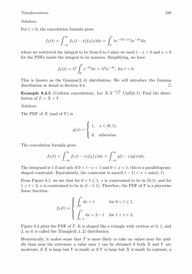
Transformations 349
Solution:
For t > 0, the convolution formula gives
fT (t) =
Z 1
�1fY (t� x)fX(x)dx =
Z t
0
�e��(t�x)�e��xdx,
where we restricted the integral to be from 0 to t since we need t�x > 0 and x > 0for the PDFs inside the integral to be nonzero. Simplifying, we have
fT (t) = �2Z t
0
e��tdx = �2te��t, for t > 0.
This is known as the Gamma(2,�) distribution. We will introduce the Gammadistribution in detail in Section 8.4. ⇤Example 8.2.5 (Uniform convolution). Let X,Y
i.i.d.⇠ Unif(0, 1). Find the distri-bution of T = X + Y .
Solution:
The PDF of X (and of Y ) is
g(x) =
8><
>:
1, x 2 (0, 1),
0, otherwise.
The convolution formula gives
fT (t) =
Z 1
�1fY (t� x)fX(x)dx =
Z 1
�1g(t� x)g(x)dx.
The integrand is 1 if and only if 0 < t�x < 1 and 0 < x < 1; this is a parallelogram-shaped constraint. Equivalently, the constraint is max(0, t� 1) < x < min(t, 1).
From Figure 8.1, we see that for 0 < t 1, x is constrained to be in (0, t), and for1 < t < 2, x is constrained to be in (t�1, 1). Therefore, the PDF of T is a piecewiselinear function:
fT (t) =
8>>><
>>>:
Z t
0
dx = t for 0 < t 1,
Z1
t�1
dx = 2� t for 1 < t < 2.
Figure 8.2 plots the PDF of T . It is shaped like a triangle with vertices at 0, 1, and2, so it is called the Triangle(0, 1, 2) distribution.
Heuristically, it makes sense that T is more likely to take on values near the mid-dle than near the extremes: a value near 1 can be obtained if both X and Y aremoderate, if X is large but Y is small, or if Y is large but X is small. In contrast, a

350 Introduction to Probability
0.0 0.5 1.0 1.5 2.0
0.0
0.2
0.4
0.6
0.8
1.0
t
x
FIGURE 8.1
Region in the (t, x)-plane where g(t� x)g(x) is 1.
0.0 0.5 1.0 1.5 2.0
0.0
0.2
0.4
0.6
0.8
1.0
t
FIGURE 8.2
PDF of T = X + Y , where X and Y are i.i.d. Unif(0, 1).

Transformations 351
value near 2 is only possible if both X and Y are large. Thinking back to Example3.2.5, the PMF of the sum of two die rolls was also shaped like a triangle. A singledie roll has a Discrete Uniform distribution on the integers 1 through 6, so in thatproblem we were looking at a convolution of two Discrete Uniforms. So it makessense that the PDF we obtained here is similar in shape. ⇤
8.3 Beta
In this section and the next, we will introduce two continuous distributions, theBeta and Gamma, which are related to several named distributions we have alreadystudied and are also related to each other via a shared story. This is an interludefrom the subject of transformations, but we’ll eventually need to use a change ofvariables to tie the Beta and Gamma distributions together.
The Beta distribution is a continuous distribution on the interval (0, 1). It is ageneralization of the Unif(0, 1) distribution, allowing the PDF to be non-constanton (0, 1).
Definition 8.3.1 (Beta distribution). An r.v.X is said to have the Beta distributionwith parameters a and b, a > 0 and b > 0, if its PDF is
f(x) =1
�(a, b)xa�1(1� x)b�1, 0 < x < 1,
where the constant �(a, b) is chosen to make the PDF integrate to 1. We write thisas X ⇠ Beta(a, b).
Taking a = b = 1, the Beta(1, 1) PDF is constant on (0, 1), so the Beta(1, 1) andUnif(0, 1) distributions are the same. By varying the values of a and b, we get PDFswith a variety of shapes; Figure 8.3 shows four examples. Here are a couple of generalpatterns:
• If a < 1 and b < 1, the PDF is U-shaped and opens upward. If a > 1 and b > 1,the PDF opens down.
• If a = b, the PDF is symmetric about 1/2. If a > b, the PDF favors values largerthan 1/2; if a < b, the PDF favors values smaller than 1/2.
By definition, the constant �(a, b) satisfies
�(a, b) =
Z1
0
xa�1(1� x)b�1dx.
An integral of this form is called a beta integral, and we will need to do some calculusto derive a general formula for �(a, b). But in the special case where a and b arepositive integers, Thomas Bayes figured out how to do the integral using a storyproof rather than calculus!

352 Introduction to Probability
0.0 0.2 0.4 0.6 0.8 1.0
01
23
45
Beta(0.5, 0.5)
x
0.0 0.2 0.4 0.6 0.8 1.0
0.0
0.5
1.0
1.5
2.0
Beta(2, 1)
x
0.0 0.2 0.4 0.6 0.8 1.0
Beta(2, 8)
x
01
23
0.0 0.2 0.4 0.6 0.8 1.0
0.0
0.5
1.0
1.5
2.0
2.5
Beta(5, 5)
x
FIGURE 8.3
Beta PDFs for various values of a and b. Clockwise from top left: Beta(0.5, 0.5),Beta(2, 1), Beta(5, 5), Beta(2, 8).

Transformations 353
Story 8.3.2 (Bayes’ billiards). Show without using calculus that for any integers kand n with 0 k n,
Z1
0
✓n
k
◆xk(1� x)n�kdx =
1
n+ 1.
Solution:
By telling two stories, we will show that the left-hand and right-hand sides are bothequal to P (X = k), where X is an r.v. that we will construct.
Story 1 : Start with n+1 balls, n white and 1 gray. Randomly throw each ball ontothe unit interval [0, 1], such that the positions of the balls are i.i.d. Unif(0, 1). LetX be the number of white balls to the left of the gray ball;X is a discrete r.v. withpossible values 0, 1, . . . , n. Figure 8.4 illustrates the setup of our experiment.
To get the probability of the event X = k, we use LOTP, conditioning on theposition of the gray ball, which we’ll call B. Conditional on B = p, the numberof white balls landing to the left of p has a Bin(n, p) distribution, since we canconsider each of the white balls to be an independent Bernoulli trial, wheresuccess is defined as landing to the left of p. Let f be the PDF of B; f(p) = 1since B ⇠ Unif(0, 1). So
P (X = k) =
Z1
0
P (X = k|B = p)f(p)dp =
Z1
0
✓n
k
◆pk(1� p)n�kdp.
0 1
FIGURE 8.4
Bayes’ billiards. Here we throw n = 6 white balls and one gray ball onto the unitinterval, and we observe X = 2 balls to the left of the gray ball.
Story 2 : Start with n + 1 balls, all white. Randomly throw each ball onto theunit interval; then choose one ball at random and paint it gray. Again, let X bethe number of white balls to the left of the gray ball. By symmetry, any one ofthe n+ 1 balls is equally likely to be painted gray, so
P (X = k) =1
n+ 1
for k = 0, 1, . . . , n.
Here’s the crux: X has the same distribution in the two stories! It does not matterwhether we paint the gray ball first and then throw, or whether we throw first andthen paint the gray ball. So P (X = k) is the same in Story 1 and Story 2, and
Z1
0
✓n
k
◆pk(1� p)n�kdp =
1
n+ 1

354 Introduction to Probability
for k = 0, 1, . . . , n. Despite the k’s in the integrand, the value of the integral doesn’tdepend on k. Substituting a�1 for k and b�1 for n�k, this shows that for positiveinteger values of a and b,
�(a, b) =1
(a+ b� 1)�a+b�2
a�1
� =(a� 1)!(b� 1)!
(a+ b� 1)!.
Later in this chapter, we’ll learn what �(a, b) is for general a and b. ⇤The Beta is a flexible family of distributions on (0, 1), and has many stories. One ofthese stories is that a Beta r.v. is often used to represent an unknown probability.That is, we can use the Beta to put probabilities on unknown probabilities!
Story 8.3.3 (Beta-Binomial conjugacy). We have a coin that lands Heads withprobability p, but we don’t know what p is. Our goal is to infer the value of pafter observing the outcomes of n tosses of the coin. The larger that n is, the moreaccurately we should be able to estimate p.
There are several ways to go about doing this. One major approach is Bayesianinference, which treats all unknown quantities as random variables. In the Bayesianapproach, we would treat the unknown probability p as a random variable and givep a distribution. This is called a prior distribution, and it reflects our uncertaintyabout the true value of p before observing the coin tosses. After the experiment isperformed and the data are gathered, the prior distribution is updated using Bayes’rule; this yields the posterior distribution, which reflects our new beliefs about p.
Let’s see what happens if the prior distribution on p is a Beta distribution. Letp ⇠ Beta(a, b) for known constants a and b, and let X be the number of heads inn tosses of the coin. Conditional on knowing the true value of p, the tosses wouldjust be independent Bernoulli trials with probability p of success, so
X|p ⇠ Bin(n, p).
Note that X is not marginally Binomial; it is conditionally Binomial, given p. Themarginal distribution of X is called the Beta-Binomial distribution. To get theposterior distribution of p, we use Bayes’ rule (in a hybrid form, since X is discreteand p is continuous). Letting f(p) be the prior distribution and f(p|X = k) be theposterior distribution after observing k Heads,
f(p|X = k) =P (X = k|p)f(p)
P (X = k)
=
✓n
k
◆pk(1� p)n�k · 1
�(a, b)pa�1(1� p)b�1
P (X = k).
The denominator, which is the marginal PMF of X, is given by
P (X = k) =
Z1
0
P (X = k|p)f(p)dp =
Z1
0
✓n
k
◆pk(1� p)n�kf(p)dp.

Transformations 355
For a = b = 1 (which gives a Unif(0, 1) prior on p), we showed in the Bayes’ billiardsstory that P (X = k) = 1/(n+ 1), i.e., X is Discrete Uniform on {0, 1, . . . , n}. Butit does not seem easy to find P (X = k) in general and, relatedly, we still have notevaluated �(a, b) in general. Are we stuck?
Actually, the calculation is much easier than it appears at first. The conditionalPDF f(p|X = k) is a function of p, which means everything that doesn’t dependon p is just a constant. We can drop all these constants and find the PDF up to amultiplicative constant (and then the normalizing constant is whatever it needs tobe to make the PDF integrate to 1). This gives
f(p|X = k) / pa+k�1(1� p)b+n�k�1,
which is the Beta(a+ k, b+n� k) PDF, up to a multiplicative constant. Therefore,the posterior distribution of p is
p|X = k ⇠ Beta(a+ k, b+ n� k).
The posterior distribution of p after observing X = k is still a Beta distribution!This is a special relationship between the Beta and Binomial distributions calledconjugacy : if we have a Beta prior distribution on p and data that are conditionallyBinomial given p, then when going from prior to posterior, we don’t leave the familyof Beta distributions. We say that the Beta is the conjugate prior of the Binomial.
Furthermore, notice the very simple formula for updating the distribution of p. Wejust add the number of observed successes, k, to the first parameter of the Betadistribution, and the number of observed failures, n � k, to the second parameter.So a and b have a concrete interpretation in this context: think of a as the numberof prior successes and b as the number of prior failures in earlier experiments.
As in Section 2.6, we can sequentially update our beliefs as we get more and moreevidence: we start with a prior distribution and update it to get a posterior distri-bution, which becomes the new prior distribution, which we update to get a newposterior distribution, etc. The beauty here is that all of this can be done within theBeta family of distributions, with easy updates to the parameters based on tallyingthe observed successes and failures.
For concreteness, Figure 8.5 shows the case where the prior is Beta(1, 1) (equivalentto Unif(0, 1), as noted earlier), and we observe n = 5 coin tosses, all of which happento land Heads. Then the posterior is Beta(6, 1), which is plotted on the right halfof Figure 8.5. Notice how the posterior distribution incorporates the evidence fromthe coin tosses: larger values of p have higher density, consistent with the fact thatwe observed all Heads.
This model is a continuous analog of Example 2.3.7, our very first example of Bayes’rule. In that example, we also had a coin whose probability of Heads p was unknown,but our prior information led us to believe that p could only take on one of two

356 Introduction to Probability
0.0 0.2 0.4 0.6 0.8 1.0
0.6
0.8
1.0
1.2
1.4
p
prio
r PD
F
0.0 0.2 0.4 0.6 0.8 1.0
01
23
45
6
p
post
erio
r PD
FFIGURE 8.5
Beta is conjugate prior of Binomial. (a) Prior is Unif(0, 1). (b) After observing 5Heads in 5 tosses, posterior is Beta(6, 1).
possible values, 1/2 or 3/4. For this reason, our prior distribution on p—though wedidn’t call it that at the time!—was discrete. In particular, our prior PMF was
P (p = 1/2) = 1/2,
P (p = 3/4) = 1/2.
After observing three Heads in a row, we updated this PMF to obtain the posteriorPMF, which assigned a probability of 0.23 to p = 1/2 and a probability of 0.77to p = 3/4. The same logic applies to the example in this chapter, except that wenow give p a continuous prior distribution, which is appropriate if we believe thatp could possibly take on any value between 0 and 1. ⇤
8.4 Gamma
The Gamma distribution is a continuous distribution on the positive real line; it is ageneralization of the Exponential distribution. While an Exponential r.v. representsthe waiting time for the first success under conditions of memorylessness, we shallsee that a Gamma r.v. represents the total waiting time for multiple successes.
Before writing down the PDF, we first introduce the gamma function, a very famousfunction in mathematics that extends the factorial function beyond the realm ofnonnegative integers.

Transformations 357
Definition 8.4.1 (Gamma function). The gamma function � is defined by
�(a) =
Z 1
0
xae�x dx
x,
for real numbers a > 0.
We could also cancel an x and write the integrand as xa�1e�x, but it turns out to beconvenient having the dx
x since it is common to make a transformation of the form
u = cx, and then we have the handy fact that duu = dx
x . Here are two importantproperties of the gamma function.
• �(a+ 1) = a�(a) for all a > 0. This follows from integration by parts:
�(a+ 1) =
Z 1
0
xae�xdx = �xae�x
����1
0
+ a
Z 1
0
xa�1e�xdx = 0 + a�(a).
• �(n) = (n�1)! if n is a positive integer. This can be proved by induction, startingwith n = 1 and using the recursive relation �(a+1) = a�(a). Thus, if we evaluatethe gamma function at positive integer values, we recover the factorial function(albeit shifted by 1).
Now let’s suppose that on a whim, we decide to divide both sides of the abovedefinition by �(a). We have
1 =
Z 1
0
1
�(a)xae�xdx
x,
so the function under the integral is a valid PDF supported on (0,1). This is thedefinition of the PDF of the Gamma distribution. Specifically, we say that X hasthe Gamma distribution with parameters a and 1, denoted X ⇠ Gamma(a, 1), if itsPDF is
fX(x) =1
�(a)xae�x 1
x, x > 0.
From the Gamma(a, 1) distribution, we obtain the general Gamma distributionby a scale transformation: if X ⇠ Gamma(a, 1) and � > 0, then the distribution ofY = X/� is called the Gamma(a,�) distribution. By the change of variables formulawith x = �y and dx/dy = �, the PDF of Y is
fY (y) = fX(x)
����dx
dy
���� =1
�(a)(�y)ae��y 1
�y� =
1
�(a)(�y)ae��y 1
y, y > 0.
This is summarized in the following definition.
Definition 8.4.2 (Gamma distribution). An r.v. Y is said to have the Gammadistribution with parameters a and �, a > 0 and � > 0, if its PDF is
f(y) =1
�(a)(�y)ae��y 1
y, y > 0.
We write Y ⇠ Gamma(a,�).

358 Introduction to Probability
Taking a = 1, the Gamma(1,�) PDF is f(y) = �e��y for y > 0, so the Gamma(1,�)and Expo(�) distributions are the same. The extra parameter a allows GammaPDFs to have a greater variety of shapes. Figure 8.6 shows four Gamma PDFs. Forsmall values of a, the PDF is skewed, but as a increases, the PDF starts to lookmore symmetrical and bell-shaped; we will learn the reason for this in Chapter 10.Increasing � compresses the PDF toward smaller values, as we can see by comparingthe Gamma(3, 1) and Gamma(3, 0.5) PDFs.
0 5 10 15 20
Gamma(3, 1)
x
0.0
0.1
0.2
0 5 10 15 20
Gamma(3, 0.5)
x
0.00
0.05
0.10
0 5 10 15 20
Gamma(10, 1)
x
0.00
0.05
0.10
0 5 10 15 20
Gamma(5, 0.5)
x
0.00
0.05
0.10
FIGURE 8.6
Gamma PDFs for various values of a and �. Clockwise from top left: Gamma(3, 1),Gamma(3, 0.5), Gamma(5, 0.5), Gamma(10, 1).
Let’s find the mean, variance, and other moments of the Gamma distribution, start-ing with X ⇠ Gamma(a, 1). We’ll use properties of the gamma function as well asthe technique of doing integrals by pattern recognition. For the mean, we write down

Transformations 359
the definition of E(X),
E(X) =
Z 1
0
1
�(a)xa+1e�xdx
x,
but instead of attempting a gruesome integration by parts, we recognize that aftertaking out 1/�(a), what’s left is precisely the gamma function evaluated at a + 1.Therefore
E(X) =�(a+ 1)
�(a)=
a�(a)
�(a)= a.
Similarly, for the variance, LOTUS gives us an integral expression for the secondmoment,
E(X2) =
Z 1
0
1
�(a)xa+2e�xdx
x,
and we recognize the gamma function evaluated at a+ 2. Therefore
E(X2) =�(a+ 2)
�(a)=
(a+ 1)a�(a)
�(a)= (a+ 1)a
andVar(X) = (a+ 1)a� a2 = a.
So for X ⇠ Gamma(a, 1), E(X) = Var(X) = a.
The cth moment is no harder than the second moment; we just use LOTUS andrecognize the definition of �(a+ c). This gives
E(Xc) =
Z 1
0
1
�(a)xa+ce�xdx
x=
�(a+ c)
�(a)
for c such that the integral converges, i.e., for c > �a.
With the results for X in hand, we can transform to Y = X/� ⇠ Gamma(a,�) toget
E(Y ) =1
�E(X) =
a
�,
Var(Y ) =1
�2Var(X) =
a
�2,
E(Y c) =1
�cE(Xc) =
1
�c· �(a+ c)
�(a), c > �a.
Looking back at the Gamma PDF plots, they are consistent with our finding thatthe mean and variance are increasing in a and decreasing in �.
So far, we’ve been learning about the Gamma distribution using the PDF, whichallowed us to discern general patterns from PDF plots and to derive the meanand variance. But the PDF doesn’t provide much insight about why we’d ever usethe Gamma distribution, and it doesn’t give us much of an interpretation for the

360 Introduction to Probability
parameters a and �. For this, we need to connect the Gamma to other nameddistributions through stories. The rest of this section is devoted to stories for theGamma distribution.
In the special case where a is an integer, we can represent a Gamma(a,�) r.v. asa sum of i.i.d. Expo(�) r.v.s (a convolution, in the fancy language of this chap-ter).
Theorem 8.4.3. Let X1
, . . . , Xn be i.i.d. Expo(�). Then
X1
+ · · ·+Xn ⇠ Gamma(n,�).
Proof. The MGF of an Expo(�) r.v. is ���t for t < �, so the MGF of X
1
+ · · ·+Xn
is
Mn(t) =
✓�
�� t
◆n
for t < �. Let Y ⇠ Gamma(n,�); we’ll show that the MGF of Y is the same as thatof X
1
+ · · ·+Xn. By LOTUS,
E(etY ) =
Z 1
0
ety1
�(n)(�y)ne��y dy
y.
Again, we’ll use the trick of integration by pattern recognition. We just need todo algebraic manipulations until what is left inside the integral is a recognizableGamma PDF:
E(etY ) =
Z 1
0
ety1
�(n)(�y)ne��y dy
y
=�n
(�� t)n
Z 1
0
1
�(n)e�(��t)y((�� t)y)n
dy
y.
We pulled �n out of the integral, then multiplied by (��t)n on the inside while divid-ing by it on the outside. Now the expression inside the integral is the Gamma(n,��t)PDF, assuming t < �. Since PDFs integrate to 1, we have
E(etY ) =
✓�
�� t
◆n
for t < �; if t � � the integral fails to converge.
We have shown that X1
+ · · · + Xn and Y ⇠ Gamma(n,�) have the same MGF.Since the MGF determines the distribution, X
1
+ · · ·+Xn ⇠ Gamma(n,�). ⌅
Thus, if Y ⇠ Gamma(a,�) with a an integer, we can represent Y as a sum ofi.i.d. Expo(�) r.v.s, X
1
+ · · ·+Xa, and get the mean and variance right away:
E(Y ) = E(X1
+ · · ·+Xa) = aE(X1
) =a
�,
Var(Y ) = Var(X1
+ · · ·+Xa) = aVar(X1
) =a
�2,

Transformations 361
in agreement with the results we derived earlier for general a.
Theorem 8.4.3 also allows us to connect the Gamma distribution to the story of thePoisson process. We showed in Chapter 5 that in a Poisson process of rate �, theinterarrival times are i.i.d. Expo(�) r.v.s. But the total waiting time Tn for the ntharrival is the sum of the first n interarrival times; for instance, Figure 8.7 illustrateshow T
3
is the sum of the 3 interarrival times X1
, X2
, X3
. Therefore, by the theorem,Tn ⇠ Gamma(n,�). The interarrival times in a Poisson process are Exponentialr.v.s, while the raw arrival times are Gamma r.v.s.
0 T1 T2 T3 T4 T5
X1 X2 X3...
+ + + + +
FIGURE 8.7
Poisson process. The interarrival times Xj are i.i.d. Expo(�), while the raw arrivaltimes Tj are Gamma(j,�).
h 8.4.4. Unlike the Xj , the Tj are not independent, since they are constrained tobe increasing; nor are they identically distributed.
At last, we have an interpretation for the parameters of the Gamma(a,�) distribu-tion. In the Poisson process story, a is the number of successes we are waiting for,and � is the rate at which successes arrive; Y ⇠ Gamma(a,�) is the total waitingtime for the ath arrival in a Poisson process of rate �.
A consequence of this story is that a convolution of Gammas with the same � isstill Gamma. Exercise 30 explores this fact from several perspectives.
When we introduced the Exponential distribution, we viewed it as the continuousanalog of the Geometric distribution: the Geometric waits for the first success indiscrete time, and the Exponential waits for the first success in continuous time.Likewise, we can now say that the Gamma distribution is the continuous analog ofthe Negative Binomial distribution: the Negative Binomial is a sum of Geometricwaiting times, and the Gamma is a sum of Exponential waiting times. In Exercise54 you will use MGFs to show that the Gamma distribution can be obtained as acontinuous limit of the Negative Binomial distribution.
A final story about the Gamma is that it shares the same special relationship withthe Poisson that the Beta shares with the Binomial: the Gamma is the conjugateprior of the Poisson. Earlier we saw that the Beta distribution can represent an un-known probability of success because its support is (0, 1). The Gamma distribution,on the other hand, can represent an unknown rate in a Poisson process because itssupport is (0,1).
362 Introduction to Probability
To investigate, we’ll return to Blotchville, where buses arrive in a Poisson process ofrate �. Previously it was assumed that � = 1/10, so that the times between buseswere i.i.d. Exponentials with mean 10 minutes, but now we’ll assume Fred doesn’tknow the rate � at which buses arrive and needs to figure it out. Fred will followthe Bayesian approach and treat the unknown rate as a random variable.
Story 8.4.5 (Gamma-Poisson conjugacy). In Blotchville, buses arrive at a certainbus stop according to a Poisson process with rate � buses per hour, where � isunknown. Based on his very memorable adventures in Blotchville, Fred quantifieshis uncertainty about � using the prior � ⇠ Gamma(r
0
, b0
), where r0
and b0
areknown, positive constants with r
0
an integer.
To better understand the bus system, Fred wants to learn more about �. He is avery patient person, and decides that he will sit at the bus stop for t hours andcount how many buses arrive in this time interval. Let Y be the number of buses inthis time interval, and suppose Fred observes that Y = y.
(a) Find Fred’s hybrid joint distribution for Y and �.
(b) Find Fred’s marginal distribution for Y .
(c) Find Fred’s posterior distribution for �, i.e., his conditional distribution of �given the data y.
(d) Find Fred’s posterior mean E(�|Y = y) and posterior variance Var(�|Y = y).
Solution:
Notice the similarities between the structure of this problem and that of Example7.1.25, the hybrid joint distribution from Chapter 7. We know � ⇠ Gamma(r
0
, b0
)marginally, and by the definition of Poisson process, conditional on knowing thetrue rate �, the number of buses in an interval of length t is distributed Pois(�t).In other words, what we’re given is
� ⇠ Gamma(r0
, b0
)
Y |� ⇠ Pois(�t).
Then we are asked to flip it around: find the marginal distribution of Y and theconditional distribution of � given Y = y, which is the posterior distribution. Thisis characteristic of Bayesian inference: we have a prior distribution for the unknownparameters (in this case, a Gamma distribution for �) and a model for the dataconditional on the unknown parameters (in this case, a Poisson distribution for Ygiven �), and we use Bayes’ rule to get the distribution of the unknowns conditionalon the observed data. So let’s get started.
(a) Let f0
be the prior PDF of �. The hybrid joint distribution of Y and � is
f(y,�) = P (Y = y|�)f0
(�) =e��t(�t)y
y!
(b0
�)r0e�b0
�
��(r0
),

Transformations 363
for y = 0, 1, 2, . . . and � > 0. The hybrid joint distribution is plotted in Figure 8.8;there is a conditional PMF of Y for every value of � and a conditional PDF of �for every value of Y .
y
!
●
●
●
● ● ● ●
FIGURE 8.8
Hybrid joint distribution of Y and �. (a) Conditioning on a particular value of �,the relative heights form a Poisson PMF. (b) In the other direction, conditioningon Y = y gives the posterior distribution of �; this is what we’re after.
(b) To get the marginal PMF of Y , we integrate out � from the hybrid joint distri-bution; this is also a form of LOTP. This gives
P (Y = y) =
Z 1
0
P (Y = y|�)f0
(�)d�
=
Z 1
0
e��t(�t)y
y!
(b0
�)r0e�b0
�
�(r0
)
d�
�.
Let’s do the integral by pattern recognition, focusing in on the terms involving�. We spot �r0+y and e�(b
0
+t)� lurking in the integrand, which suggests pattern-matching to a Gamma(r
0
+y, b0
+ t) PDF. Pull out all the terms that don’t dependon �, then multiply by whatever it takes to get the desired PDF inside the integral,

364 Introduction to Probability
remembering to multiply by the reciprocal on the outside:
P (Y = y) =tybr0
0
y!�(r0
)
Z 1
0
e�(b0
+t)��r0+y d�
�
=�(r
0
+ y)
y!�(r0
)
tybr00
(b0
+ t)r0+y
Z 1
0
1
�(r0
+ y)e�(b
0
+t)�((b0
+ t)�)r0+y d�
�
=(r
0
+ y � 1)!
(r0
� 1)!y!
✓t
b0
+ t
◆y ✓ b0
b0
+ t
◆r0
.
In the last step, we used the property �(n) = (n � 1)!, applicable because r0
is aninteger. This is the NBin(r
0
, b0
/(b0
+ t)) PMF, so the marginal distribution of Y isNegative Binomial with parameters r
0
and b0
/(b0
+ t).
(c) By Bayes’ rule, the posterior PDF of � is given by
f1
(�|y) = P (Y = y|�)f0
(�)
P (Y = y).
We found P (Y = y) in the previous part, but since it does not depend on �, wecan just treat it as part of the normalizing constant. Absorbing this and othermultiplicative factors that don’t depend on � into the normalizing constant, wehave
f1
(�|y) / e��t�y�r0e�b0
� 1
�= e�(b
0
+t)��r0+y 1
�,
which shows that the posterior distribution of � is Gamma(r0
+ y, b0
+ t).
When going from prior to posterior, the distribution of � stays in the Gamma family,so the Gamma is indeed the conjugate prior for the Poisson.
(d) Since conditional PDFs are PDFs, it is perfectly fine to calculate the expectationand variance of � with respect to the posterior distribution. The mean and varianceof the Gamma(r
0
+ y, b0
+ t) distribution give us
E(�|Y = y) =r0
+ y
b0
+ tand Var(�|Y = y) =
r0
+ y
(b0
+ t)2.
This example gives another interpretation for the parameters in a Gamma distri-bution when it is being used as a conjugate prior. Fred’s Gamma(r
0
, b0
) prior gotupdated to a Gamma(r
0
+ y, b0
+ t) posterior after observing y arrivals in t hours.We can imagine that in the past, Fred observed r
0
buses arrive in b0
hours; thenafter the new data, he has observed r
0
+y buses in b0
+ t hours. So we can interpretr0
as the number of prior arrivals and b0
as the total time required for those priorarrivals. ⇤

Transformations 365
8.5 Beta-Gamma connections
In this section, we will unite the Beta and Gamma distributions with a commonstory. As an added bonus, the story will give us an expression for the normalizingconstant of the Beta(a, b) PDF in terms of gamma functions, and it will allow us toeasily find the expectation of the Beta(a, b) distribution.
Story 8.5.1 (Bank–post o�ce). While running errands, you need to go to thebank, then to the post o�ce. Let X ⇠ Gamma(a,�) be your waiting time in lineat the bank, and let Y ⇠ Gamma(b,�) be your waiting time in line at the posto�ce (with the same � for both). Assume X and Y are independent. What is thejoint distribution of T = X + Y (your total wait at the bank and post o�ce) andW = X
X+Y (the fraction of your waiting time spent at the bank)?
Solution:
We’ll do a change of variables in two dimensions to get the joint PDF of T and W .Let t = x+ y, w = x
x+y . Then x = tw, y = t(1� w), and
@(x, y)
@(t, w)=
0
B@w t
1� w �t
1
CA ,
which has an absolute determinant of t. Therefore
fT,W (t, w) = fX,Y (x, y) ·����@(x, y)
@(t, w)
����
= fX(x)fY (y) · t
=1
�(a)(�x)ae��x 1
x· 1
�(b)(�y)be��y 1
y· t
=1
�(a)(�tw)ae��tw 1
tw· 1
�(b)(�t(1� w))be��t(1�w)
1
t(1� w)· t.
Let’s group all the terms involving w together, and all the terms involving t together:
fT,W (t, w) =1
�(a)�(b)wa�1(1� w)b�1(�t)a+be��t 1
t
=
✓�(a+ b)
�(a)�(b)wa�1(1� w)b�1
◆✓1
�(a+ b)(�t)a+be��t 1
t
◆,
for 0 < w < 1 and t > 0. The form of the joint PDF, together with Proposi-tion 7.1.20, tells us several things:
1. Since the joint PDF factors into a function of t times a function of w, we havethat T and W are independent: the total waiting time is independent of the fractionof time spent at the bank.

366 Introduction to Probability
2. We recognize the marginal PDF of T and deduce that T ⇠ Gamma(a+ b,�).
3. The PDF of W is
fW (w) =�(a+ b)
�(a)�(b)wa�1(1� w)b�1, 0 < w < 1,
by Proposition 7.1.20 or just by integrating out T from the joint PDF of T andW . This PDF is proportional to the Beta(a, b) PDF, so it is the Beta(a, b) PDF!Note that as a byproduct of the calculation we have just done, we have found thenormalizing constant of the Beta distribution:
1
�(a, b)=
�(a+ b)
�(a)�(b)
is the constant that goes in front of the Beta(a, b) PDF. ⇤To summarize, the bank–post o�ce story tells us that when we add independentGamma r.v.s X and Y with the same rate �, the total X+Y has a Gamma distribu-tion, the fraction X/(X + Y ) has a Beta distribution, and the total is independentof the fraction.
We can use this result to find the mean of W ⇠ Beta(a, b) without the slightesttrace of calculus. Since T and W are independent, they are uncorrelated: E(TW ) =E(T )E(W ). Writing this in terms of X and Y , we have
E
✓(X + Y ) · X
X + Y
◆= E(X + Y )E
✓X
X + Y
◆,
E(X) = E(X + Y )E
✓X
X + Y
◆,
E(X)
E(X + Y )= E
✓X
X + Y
◆.
Ordinarily, the last equality would be a horrendous blunder: faced with an expec-tation like E(X/(X + Y )), we are not generally permitted to move the E into thenumerator and denominator as we please. In this case, however, the bank–post o�cestory justifies the move, so finding the expectation of W happily reduces to findingthe expectations of X and X + Y :
E(W ) = E
✓X
X + Y
◆=
E(X)
E(X + Y )=
a/�
a/�+ b/�=
a
a+ b.
Another approach is to proceed from the definition of expectation:
E(W ) =
Z1
0
�(a+ b)
�(a)�(b)wa(1� w)b�1dw,
and by pattern recognition, the integrand is a Beta(a+1, b) PDF, up to a normalizing

Transformations 367
constant. After obtaining an exact match for the PDF, we apply properties of thegamma function:
E(W ) =�(a+ b)
�(a)
�(a+ 1)
�(a+ b+ 1)
Z1
0
�(a+ b+ 1)
�(a+ 1)�(b)wa(1� w)b�1dw
=�(a+ b)
�(a)
a�(a)
(a+ b)�(a+ b)
=a
a+ b.
In Exercise 31, you will use this approach to find the variance and the other momentsof the Beta distribution.
8.6 Order statistics
The final transformation we will consider in this chapter is the transformationthat takes n random variables X
1
, . . . , Xn and sorts them in order, producing thetransformed r.v.s min(X
1
, . . . , Xn), . . . ,max(X1
, . . . , Xn). The transformed r.v.s arecalled the order statistics1, and they are often useful when we are concerned withthe distribution of extreme values, as we alluded to at the beginning of the chap-ter.
Furthermore, like the sample mean Xn, the order statistics serve as useful summariesof an experiment, since we can use them to determine the cuto↵s for the worst 5%of observations, the worst 25%, the best 25%, and so forth (these cuto↵s are calledquantiles).
Definition 8.6.1 (Order statistics). For r.v.s X1
, X2
, . . . , Xn, the order statisticsare the random variables X
(1)
, . . . , X(n), where
X(1)
= min(X1
, . . . , Xn),
X(2)
is the second-smallest of X1
, . . . , Xn,
...
X(n�1)
is the second-largest of X1
, . . . , Xn,
X(n) = max(X
1
, . . . , Xn).
Note that X(1)
X(2)
. . . X(n) by definition. We call X
(j) the jth orderstatistic. If n is odd, X
((n+1)/2) is called the sample median of X1
, . . . , Xn.
1This term sometimes causes confusion. In statistics (the field of study), any function of thedata is called a statistic. If X
1
, . . . , Xn are the data, then min(X1
, . . . , Xn) is a statistic, and sois max(X
1
, . . . , Xn). They are called order statistics because we get them by sorting the data inorder.

368 Introduction to Probability
h 8.6.2. The order statistics X(1)
, . . . , X(n) are random variables, and each X
(j)
is a function of X1
, . . . , Xn. Even if the original r.v.s are independent, the orderstatistics are dependent : if we know that X
(1)
= 100, then X(n) is forced to be at
least 100.
We will focus our attention on the case where X1
, . . . , Xn are i.i.d. continuous r.v.s.The reason is that with discrete r.v.s, there is a positive probability of tied values;with continuous r.v.s, the probability of a tie is exactly 0, which makes matters mucheasier. Thus, for the rest of this section, assume X
1
, . . . , Xn are i.i.d. and continuous,with CDF F and PDF f . We will derive the marginal CDF and PDF of eachindividual order statistic X
(j), as well as the joint PDF of (X(1)
, . . . , X(n)).
A complication we run into right away is that the transformation to order statisticsis not invertible: starting with min(X,Y ) = 3 and max(X,Y ) = 5, we can’t tellwhether the original values of X and Y were 3 and 5, respectively, or 5 and 3.Therefore the change of variables formula from Rn to Rn does not apply. Insteadwe will take a direct approach, using pictures to guide us when necessary.
Let’s start with the CDF of X(n) = max(X
1
, . . . Xn). Since X(n) is less than x if
and only if all of the Xj are less than x, the CDF of X(n) is
FX(n)
(x) = P (max(X1
, . . . , Xn) x)
= P (X1
x, . . . ,Xn x)
= P (X1
x) . . . P (Xn x)
= (F (x))n,
where F is the CDF of the individual Xi. Similarly, X(1)
= min(X1
, . . . , Xn) exceedsx if and only if all of the Xj exceed x, so the CDF of X
(1)
is
FX(1)
(x) = 1� P (min(X1
, . . . , Xn) > x)
= 1� P (X1
> x, . . . , Xn > x)
= 1� (1� F (x))n.
The same logic lets us find the CDF of X(j). For the event X
(j) x to occur, weneed at least j of the Xi to fall to the left of x. This is illustrated in Figure 8.9.
Since it appears that the number of Xi to the left of x will be important to us,let’s define a new random variable, N , to keep track of just that: define N tobe the number of Xi that land to the left of x. Each Xi lands to the left of xwith probability F (x), independently. If we define success as landing to the leftof x, we have n independent Bernoulli trials with probability F (x) of success, soN ⇠ Bin(n, F (x)). Then, by the Binomial PMF,
P (X(j) x) = P (at least j of the Xi are to the left of x)
= P (N � j)
=nX
k=j
✓n
k
◆F (x)k(1� F (x))n�k.

Transformations 369
x
at least j to the left of x
X(1) X(j) X(j + 1)... X(j + 2) ...
FIGURE 8.9
The event X(j) x is equivalent to the event “at least j of the Xi fall to the left of
x”.
We thus have the following result for the CDF of X(j).
Theorem 8.6.3 (CDF of order statistic). Let X1
, . . . , Xn be i.i.d. continuous r.v.swith CDF F . Then the CDF of the jth order statistic X
(j) is
P (X(j) x) =
nX
k=j
✓n
k
◆F (x)k(1� F (x))n�k.
To get the PDF of X(j), we can di↵erentiate the CDF with respect to x, but the
resulting expression is ugly (though it can be simplified). Instead we will take a moredirect approach. Consider fX
(j)
(x)dx, the probability that the jth order statistic fallsinto an infinitesimal interval of length dx around x. The only way this can happenis illustrated in Figure 8.10. We need one of the Xi to fall into the infinitesimalinterval around x, and we need exactly j�1 of the Xi to fall to the left of x, leavingthe remaining n� j to fall to the right of x.
x
j – 1 to the left of x
( )
n – j to the right of x1 in a tiny interval around x
FIGURE 8.10
In order for X(j) to fall within a small interval of x, we require that one of the Xi
fall within the small interval and that exactly j � 1 fall to the left of x.
What is the probability of this extremely specific event? Let’s break up the experi-ment into stages.
• First, we choose which one of the Xi will fall into the infinitesimal interval aroundx. There are n such choices, each of which occurs with probability f(x)dx, wheref is the PDF of the Xi.

370 Introduction to Probability
• Next, we choose exactly j � 1 out of the remaining n � 1 to fall to the left of x.There are
�n�1
j�1
�such choices, each with probability F (x)j�1(1� F (x))n�j by the
Bin(n, F (x)) PMF.
We multiply the probabilities of the two stages to get
fX(j)
(x)dx = nf(x)dx
✓n� 1
j � 1
◆F (x)j�1(1� F (x))n�j .
Dropping the dx’s from both sides gives us the PDF we desire.
Theorem 8.6.4 (PDF of order statistic). Let X1
, . . . , Xn be i.i.d. continuous r.v.swith CDF F and PDF f . Then the marginal PDF of the jth order statistic X
(j) is
fX(j)
(x) = n
✓n� 1
j � 1
◆f(x)F (x)j�1(1� F (x))n�j .
In general, the order statistics of X1
, . . . , Xn will not follow a named distribution,but the order statistics of the standard Uniform distribution are an exception.
Example 8.6.5 (Order statistics of Uniforms). Let U1
, . . . , Un be i.i.d. Unif(0, 1).Then for 0 x 1, f(x) = 1 and F (x) = x, so the PDF of U
(j) is
fU(j)
(x) = n
✓n� 1
j � 1
◆xj�1(1� x)n�j .
This is the Beta(j, n� j+1) PDF! So U(j) ⇠ Beta(j, n� j+1), and E(U
(j)) =j
n+1
.
The simple case n = 2 is consistent with Example 7.2.2, where we used 2D LOTUS toshow that for i.i.d. U
1
, U2
⇠ Unif(0, 1), E(max(U1
, U2
)) = 2/3 and E(min(U1
, U2
)) =1/3. Now that we know max(U
1
, U2
) and min(U1
, U2
) follow Beta distributions, theexpectation of the Beta distribution confirms our earlier findings. ⇤
8.7 Recap
In this chapter we discussed three broad classes of transformations:
• smooth, invertible transformations of continuous r.v.s, which can be handled withthe change of variables formula;
• convolutions, for which we can determine the distribution using (in decreasingorder of preference) stories, MGFs, or convolution sums/integrals;
• the transformation of i.i.d. continuous r.v.s to their order statistics.

Transformations 371
x
−3−2
−10
12
3y
−3
−2
−1
0
1
2
3
0.00
0.05
0.10
0.15
0.20
joint distributions random vectors events numbers
What can happen?
joint PDF fX,Y(x,y) (X,Y) P((X,Y) is in A)(X,Y) is in A,
with A a specified region in the plane
generate P
joint PDF fZ,W(z,w)(Z,W) = g(X,Y)
generate
Jaco
bian
P((Z,W) is in B)(Z,W) is in B,
whereB = {g(x,y): (x,y) is in A}
P
=(same event)
=(same probability)
integrate over B
integrate over A
trans
form
ation
FIGURE 8.11
Let (Z,W ) = g(X,Y ) be a smooth, one-to-one transformation. The change of vari-ables formula lets us go back and forth between the joint PDFs of (X,Y ) and(Z,W ). Let A be a region in the (x, y)-plane, and B = {g(x, y) : (x, y) 2 A} bethe corresponding region in the (z, w)-plane. Then (X,Y ) 2 A is the same event as(Z,W ) 2 B. To find the probability of this event, we can either integrate the jointPDF of (X,Y ) over A or integrate the joint PDF of (Z,W ) over B.
Figure 8.11 illustrates connections between the original random vector (X,Y ) andthe transformed random vector (Z,W ) = g(X,Y ), where g is a smooth, invertibletransformation. The change of variables formula uses Jacobians to take us back andforth between the joint PDF of (X,Y ) and that of (Z,W ). Let A be a region inthe (x, y)-plane, and B = {g(x, y) : (x, y) 2 A} be the corresponding region in the(z, w)-plane. Then (X,Y ) 2 A is the same event as (Z,W ) 2 B, so
P ((X,Y ) 2 A) = P ((Z,W ) 2 B).
To find this probability, we can either integrate the joint PDF of (X,Y ) over A orintegrate the joint PDF of (Z,W ) over B.
In this chapter, we made extensive use of Bayes’ rule and LOTP, often in continuousor hybrid forms, as well as the strategy of integration by pattern recognition.
The two new distributions we introduced are the Beta and Gamma, which are ladenwith stories and connections to other distributions. The Beta is a generalization ofthe Unif(0, 1) distribution, and it has the following stories.

372 Introduction to Probability
• Order statistics of the Uniform: The jth order statistic of n i.i.d. Unif(0, 1) r.v.sis distributed Beta(j, n� j + 1).
• Unknown probability, conjugate prior of the Binomial : If p ⇠ Beta(a, b) and X|p ⇠Bin(n, p), then p|X = k ⇠ Beta(a + k, b + n � k). The posterior distribution ofp stays within the Beta family of distributions after updating based on Binomialdata, a property known as conjugacy. The parameters a and b can be interpretedas the prior number of successes and failures, respectively.
The Gamma is a generalization of the Exponential distribution, and it has thefollowing stories.
• Poisson process: In a Poisson process of rate �, the total waiting time for n arrivalsis distributed Gamma(n,�). Thus the Gamma is the continuous analog of theNegative Binomial distribution.
• Unknown rate, conjugate prior of the Poisson: If � ⇠ Gamma(r0
, b0
) and Y |� ⇠Pois(�t), then �|Y = y ⇠ Gamma(r
0
+ y, b0
+ t). The posterior distribution of �stays within the Gamma family of distributions after updating based on Poissondata. The parameters r
0
and b0
can be interpreted as the prior number of observedsuccesses and the total waiting time for those successes, respectively.
The Beta and Gamma distributions are related by the bank–post o�ce story, whichsays that if X ⇠ Gamma(a,�), Y ⇠ Gamma(b,�), and X and Y are independent,then X + Y ⇠ Gamma(a + b,�), X
X+Y ⇠ Beta(a, b), and X + Y and XX+Y are
independent.
The diagram of connections, which we last saw in Chapter 5, is hereby updated toinclude the Beta and Gamma distributions. Distributions listed in parentheses arespecial cases of the ones not in parentheses.
Pois
HGeom
Bin(Bern)
Conditioning
Conditioning
Limit
Limit
Gamma(Expo)
NBin(Geom)
Poisson process
Limit
Beta(Unif)
Conjugacy
Bank - Post OfficeConjugacy

Transformations 373
8.8 R
Beta and Gamma distributions
The Beta and Gamma distributions are programmed into R.
• dbeta, pbeta, rbeta: To evaluate the Beta(a, b) PDF or CDF at x, we usedbeta(x,a,b) and pbeta(x,a,b). To generate n realizations from the Beta(a, b)distribution, we use rbeta(n,a,b).
• dgamma, pgamma, rgamma: To evaluate the Gamma(a,�) PDF or CDF at x, we usedgamma(x,a,lambda) or pgamma(x,a,lambda). To generate n realizations fromthe Gamma(a, lambda) distribution, we use rgamma(n,a,lambda).
For example, we can check that the Gamma(3, 2) distribution has mean 3/2 andvariance 3/4. To do this, we generate a large number of Gamma(3, 2) random vari-ables using rgamma, then compute their mean and var:
y <- rgamma(10^5,3,2)
mean(y)
var(y)
Did you get values that were close to 1.5 and 0.75, respectively?
Convolution of Uniforms
Using R, we can quickly verify that for X,Yi.i.d.⇠ Unif(0, 1), the distribution of
T = X + Y is triangular in shape:
x <- runif(10^5)
y <- runif(10^5)
hist(x+y)
The histogram looks like an ascending and then descending staircase, a discreteapproximation to a triangle.
Bayes’ billiards
In the Bayes’ billiards story, we have n white balls and 1 gray ball, throw them ontothe unit interval completely at random, and count the number of white balls to theleft of the gray ball. Letting p be the position of the gray ball and X be the numberof white balls to the left of the gray ball, we have
p ⇠ Unif(0, 1)
X|p ⇠ Bin(n, p).

374 Introduction to Probability
By performing this experiment a large number of times, we can verify the resultswe derived in this chapter about the marginal PMF of X and the posterior PDF ofp given X = x. We’ll let the number of simulations be called nsim, to avoid a nameconflict with the number of white balls, n, which we set equal to 10:
nsim <- 10^5
n <- 10
We simulate 105 values of p, then simulate 105 values from the conditional distri-bution of X given p:
p <- runif(nsim)
x <- rbinom(nsim,n,p)
Notice that we feed the entire vector p into rbinom. This means that the first elementof x is generated using the first element of p, the second element of x is generatedusing the second element of p, and so forth. Thus, conditional on a particularelement of p, the corresponding element of x is Binomial, but the elements of p arethemselves Uniform, exactly as the model specifies.
According to the Bayes’ billiards argument, the marginal distribution of X shouldbe Discrete Uniform on the integers 0 through n. Is this in fact the case? We canmake a histogram of x to check! Because the distribution of X is discrete, we tellR to make the histogram breaks at �0.5, 0.5, 1.5, . . . so that each bar is centered atan integer value:
hist(x,breaks=seq(-0.5,n+0.5,1))
Indeed, all the histogram bars are approximately equal in height, consistent with aDiscrete Uniform distribution.
Now for the posterior distribution of p given X = x. Conditioning is very simplein R. To consider only the simulated values of p where the value of X was 3, weuse square brackets, like this: p[x==3]. In particular, we can create a histogram ofthese values to see what the posterior distribution of p given X = 3 looks like; tryhist(p[x==3]).
According to the Beta-Binomial conjugacy result, the true posterior distributionis p|X = 3 ⇠ Beta(4, 8). We can plot the histogram of p[x==3] next to a his-togram of simulated values from the Beta(4, 8) distribution to confirm that theylook similar:
par(mfrow=c(1,2))
hist(p[x==3])
hist(rbeta(10^4,4,8))
The first line tells R we want two side-by-side plots, and the second and third linescreate the histograms.

Transformations 375
Simulating order statistics
Simulating order statistics in R is easy: we simply simulate i.i.d. r.v.s and use sortto sort them in order. For example,
sort(rnorm(10))
produces one realization of X(1)
, . . . , X(10)
, where X1
, . . . , X10
are i.i.d. N (0, 1).If we want to plot a histogram of realizations of, say, X
(9)
, we’ll need to usereplicate:
order_stats <- replicate(10^4, sort(rnorm(10)))
This creates a matrix, order_stats, with 10 rows. The ith row of the matrix con-tains 104 realizations of X
(i). Now we can create a histogram of X(9)
, simply byselecting row 9 of the matrix:
x9 <- order_stats[9,]
hist(x9)
We can also compute summaries like mean(x9) and var(x9).
8.9 Exercises
Change of variables
1. Find the PDF of e�X for X ⇠ Expo(1).
2. Find the PDF of X7 for X ⇠ Expo(�).
3. Find the PDF of Z3 for Z ⇠ N (0, 1).
4. s� Find the PDF of Z4 for Z ⇠ N (0, 1).
5. Find the PDF of |Z| for Z ⇠ N (0, 1).
6. s� Let U ⇠ Unif(0, 1). Find the PDFs of U2 andpU .
7. Let U ⇠ Unif(0, ⇡2
). Find the PDF of sin(U).
8. Let U ⇠ Unif(�⇡2
, ⇡2
). Find the PDF of tan(U).
9. (a) Find the distribution of X2 for X ⇠ DUnif(0, 1, . . . , n).
(b) Find the distribution of X2 for X ⇠ DUnif(�n,�n+ 1, . . . , 0, 1, . . . , n).
10. LetX ⇠ Bern(1/2) and let a and b be constants with a < b. Find a simple transformationof X that yields an r.v. that equals a with probability 1�p and equals b with probabilityp.
11. Let X ⇠ Pois(�) and Y be the indicator of X being odd. Find the PMF of Y .
Hint: Find P (Y = 0)�P (Y = 1) by writing P (Y = 0) and P (Y = 1) as series and thenusing the fact that (�1)k is 1 if k is even and �1 if k is odd.
12. Three students are working independently on their probability homework. They start atthe same time. The times that they take to finish it are i.i.d. random variables T
1
, T2
, T3
with T1/�j ⇠ Expo(�), where � and � are known positive constants.
(a) Find the PDF of T1
.

376 Introduction to Probability
(b) Find expressions for E(T 2
1
) as integrals in two di↵erent ways, one based on the PDFof T
1
, and the other based on the Expo(�) PDF (do not simplify).
13. Let T be the ratio X/Y of two i.i.d. N (0, 1) r.v.s. X,Y . This is the Cauchy distributionand, as shown in Example 7.1.24, it has PDF
fT (t) =1
⇡(1 + t2).
(a) Show that 1/T has the same distribution as T using calculus, after first finding theCDF of 1/T . (Note that the one-dimensional change of variables formula does not applydirectly, since the function g(t) = 1/t, even though it has g0(t) < 0 for all t 6= 0, isundefined at t = 0 and is not a strictly decreasing function on its domain.)
(b) Show that 1/T has the same distribution as T without using calculus, in 140 char-acters or fewer.
14. Let X and Y be i.i.d. Expo(�), and T = log(X/Y ). Find the CDF and PDF of T .
15. Let X and Y have joint PDF fX,Y (x, y), and transform (X,Y ) 7! (T,W ) linearly byletting
T = aX + bY and W = cX + dY,
where a, b, c, d are constants such that ad� bc 6= 0.
(a) Find the joint PDF fT,W (t, w) (in terms of fX,Y , though your answer should bewritten as a function of t and w).
(b) For the case where T = X + Y,W = X � Y , show that
fT,W (t, w) =12fX,Y
✓t+ w
2,t� w
2
◆.
16. s� Let X,Y be continuous r.v.s with a spherically symmetric joint distribution, whichmeans that the joint PDF is of the form f(x, y) = g(x2 + y2) for some function g. Let(R, ✓) be the polar coordinates of (X,Y ), so R2 = X2+Y 2 is the squared distance fromthe origin and ✓ is the angle (in [0, 2⇡)), with X = R cos ✓, Y = R sin ✓.
(a) Explain intuitively why R and ✓ are independent. Then prove this by finding thejoint PDF of (R, ✓).
(b) What is the joint PDF of (R, ✓) when (X,Y ) is Uniform in the unit disk {(x, y) :x2 + y2 1}?
(c) What is the joint PDF of (R, ✓) when X and Y are i.i.d. N (0, 1)?
17. Let X and Y be i.i.d. N (0, 1) r.v.s, T = X + Y , and W = X � Y . We know fromExample 7.5.8 that T and W are independent N (0, 2) r.v.s (note that (T,W ) is Multi-variate Normal with Cov(T,W ) = 0). Give another proof of this fact, using the changeof variables theorem.
18. Let X and Y be i.i.d. N (0, 1) r.v.s, and (R, ✓) be the polar coordinates for the point(X,Y ), so X = R cos ✓ and Y = R sin ✓ with R � 0 and ✓ 2 [0, 2⇡). Find the joint PDFof R2 and ✓. Also find the marginal distributions of R2 and ✓, giving their names (andparameters) if they are distributions we have studied before.
19. Let X and Y be independent positive r.v.s, with PDFs fX and fY respectively. Let Tbe the ratio X/Y .
(a) Find the joint PDF of T and X, using a Jacobian.
(b) Find the marginal PDF of T , as a single integral.
20. Let X and Y be i.i.d. Expo(�), and transform them to T = X + Y,W = X/Y .
(a) Find the joint PDF of T and W . Are they independent?
(b) Find the marginal PDFs of T and W .

Transformations 377
Convolutions
21. Let U ⇠ Unif(0, 1) and X ⇠ Expo(1), independently. Find the PDF of U +X.
22. Let X and Y be i.i.d. Expo(�). Use a convolution integral to show that the PDF ofL = X � Y is f(t) = 1
2
e�|t| for all real t; this is known as the Laplace distribution.
23. Use a convolution integral to show that if X ⇠ N (µ1
,�2) and Y ⇠ N (µ2
,�2) areindependent, then T = X + Y ⇠ N (µ
1
+ µ2
, 2�2) (to simplify the calculation, we areassuming that the variances are equal). You can use a standardization (location-scale)idea to reduce to the standard Normal case before setting up the integral.
Hint: Complete the square.
24. s� Let X and Y be independent positive r.v.s, with PDFs fX and fY respectively, andconsider the product T = XY . When asked to find the PDF of T , Jacobno arguesthat “it’s like a convolution, with a product instead of a sum. To have T = t we needX = x and Y = t/x for some x; that has probability fX(x)fY (t/x), so summing upthese possibilities we get that the PDF of T is
R10
fX(x)fY (t/x)dx.” Evaluate Jacobno’sargument, while getting the PDF of T (as an integral) in 2 ways:
(a) using the continuous version of the law of total probability to get the CDF, andthen taking the derivative (you can assume that swapping the derivative and integral isvalid);
(b) by taking the log of both sides of T = XY and doing a convolution (and thenconverting back to get the PDF of T ).
25. Let X and Y be i.i.d. Discrete Uniform r.v.s on {0, 1, . . . , n}, where n is a positiveinteger. Find the PMF of T = X + Y .
26. Let X and Y be i.i.d. Unif(0, 1), and let W = X � Y .
(a) Find the mean and variance of W , without yet deriving the PDF.
(b) Show that the distribution of W is symmetric about 0, without yet deriving thePDF.
(c) Find the PDF of W .
(d) Use the PDF of W to verify your results from (a) and (b).
(e) How does the distribution of W relate to the distribution of X + Y , the Triangledistribution derived in Example 8.2.5? Give a precise description, e.g., using the conceptsof location and scale.
27. Let X and Y be i.i.d. Unif(0, 1), and T = X + Y . We derived the distribution of T(a Triangle distribution) in Example 8.2.5, using a convolution integral. Since (X,Y )is Uniform in the unit square {(x, y) : 0 < x < 1, 0 < y < 1}, we can also interpretP ((X,Y ) 2 A) as the area of A, for any region A within the unit square. Use this ideato find the CDF of T , by interpreting the CDF (evaluated at some point) as an area.
28. Let X,Y, Z be i.i.d. Unif(0, 1), and W = X + Y + Z. Find the PDF of W .
Hint: We already know the PDF of X + Y . Be careful about limits of integration in theconvolution integral; there are 3 cases that should be considered separately.
Hint: In finding P (T = k), it helps to consider the cases 0 k n and n+ 1 k 2nseparately. Be careful about the range of summation in the convolution sum.
Beta and Gamma
29. s� Let B ⇠ Beta(a, b). Find the distribution of 1�B in two ways: (a) using a change ofvariables and (b) using a story proof. Also explain why the result makes sense in termsof Beta being the conjugate prior for the Binomial.

378 Introduction to Probability
30. s� Let X ⇠ Gamma(a,�) and Y ⇠ Gamma(b,�) be independent, with a and b integers.Show that X +Y ⇠ Gamma(a+ b,�) in three ways: (a) with a convolution integral; (b)with MGFs; (c) with a story proof.
31. Let B ⇠ Beta(a, b). Use integration by pattern recognition to find E(Bk) for positiveintegers k. In particular, show that
Var(B) =ab
(a+ b)2(a+ b+ 1).
32. s� Fred waits X ⇠ Gamma(a,�) minutes for the bus to work, and then waits Y ⇠Gamma(b,�) for the bus going home, with X and Y independent. Is the ratio X/Yindependent of the total wait time X + Y ?
33. s� The F -test is a very widely used statistical test based on the F (m,n) distribution,
which is the distribution of X/mY/n
with X ⇠ Gamma(m2
, 1
2
), Y ⇠ Gamma(n2
, 1
2
). Find the
distribution of mV/(n+mV ) for V ⇠ F (m,n).
34. s� Customers arrive at the Leftorium store according to a Poisson process with rate �customers per hour. The true value of � is unknown, so we treat it as a random variable.Suppose that our prior beliefs about � can be expressed as � ⇠ Expo(3). Let X be thenumber of customers who arrive at the Leftorium between 1 pm and 3 pm tomorrow.Given that X = 2 is observed, find the posterior PDF of �.
35. s� Let X and Y be independent, positive r.v.s. with finite expected values.
(a) Give an example where E( XX+Y
) 6= E(X)
E(X+Y )
, computing both sides exactly.
Hint: Start by thinking about the simplest examples you can think of!
(b) If X and Y are i.i.d., then is it necessarily true that E( XX+Y
) = E(X)
E(X+Y )
?
(c) Now let X ⇠ Gamma(a,�) and Y ⇠ Gamma(b,�). Show without using calculus that
E
✓Xc
(X + Y )c
◆=
E(Xc)E((X + Y )c)
for every real c > 0.
36. Alice walks into a post o�ce with 2 clerks. Both clerks are in the midst of servingcustomers, but Alice is next in line. The clerk on the left takes an Expo(�
1
) time toserve a customer, and the clerk on the right takes an Expo(�
2
) time to serve a customer.Let T
1
be the time until the clerk on the left is done serving his or her current customer,and define T
2
likewise for the clerk on the right.
(a) If �1
= �2
, is T1
/T2
independent of T1
+ T2
?
Hint: T1
/T2
= (T1
/(T1
+ T2
))/(T2
/(T1
+ T2
)).
(b) Find P (T1
< T2
) (do not assume �1
= �2
here or in the next part, but do checkthat your answers make sense in that special case).
(c) Find the expected total amount of time that Alice spends in the post o�ce (assumingthat she leaves immediately after she is done being served).
37. Let X ⇠ Pois(�t) and Y ⇠ Gamma(j,�), where j is a positive integer. Show using astory about a Poisson process that
P (X � j) = P (Y t).
38. Visitors arrive at a certain scenic park according to a Poisson process with rate �visitors per hour. Fred has just arrived (independent of anyone else), and will stay foran Expo(�
2
) number of hours. Find the distribution of the number of other visitors whoarrive at the park while Fred is there.

Transformations 379
39. (a) Let p ⇠ Beta(a, b), where a and b are positive real numbers. Find E(p2(1 � p)2),fully simplified (� should not appear in your final answer).
Two teams, A and B, have an upcoming match. They will play five games and thewinner will be declared to be the team that wins the majority of games. Given p, theoutcomes of games are independent, with probability p of team A winning and 1 � pof team B winning. But you don’t know p, so you decide to model it as an r.v., withp ⇠ Unif(0, 1) a priori (before you have observed any data).
To learn more about p, you look through the historical records of previous games betweenthese two teams, and find that the previous outcomes were, in chronological order,AAABBAABAB. (Assume that the true value of p has not been changing over timeand will be the same for the match, though your beliefs about p may change over time.)
(b) Does your posterior distribution for p, given the historical record of games betweenA and B, depend on the specific order of outcomes or only on the fact that A wonexactly 6 of the 10 games on record? Explain.
(c) Find the posterior distribution for p, given the historical data.
The posterior distribution for p from (c) becomes your new prior distribution, and thematch is about to begin!
(d) Conditional on p, is the indicator of A winning the first game of the match positivelycorrelated with, uncorrelated with, or negatively correlated of the indicator of A winningthe second game of the match? What about if we only condition on the historical data?
(e) Given the historical data, what is the expected value for the probability that thematch is not yet decided when going into the fifth game (viewing this probability as anr.v. rather than a number, to reflect our uncertainty about it)?
40. An engineer is studying the reliability of a product by performing a sequence of ntrials. Reliability is defined as the probability of success. In each trial, the productsucceeds with probability p and fails with probability 1� p. The trials are conditionallyindependent given p. Here p is unknown (else the study would be unnecessary!). Theengineer takes a Bayesian approach, with p ⇠ Unif(0, 1) as prior.
Let r be a desired reliability level and c be the corresponding confidence level, in thesense that, given the data, the probability is c that the true reliability p is at least r. Forexample, if r = 0.9, c = 0.95, we can be 95% sure, given the data, that the product isat least 90% reliable. Suppose that it is observed that the product succeeds all n times.Find a simple equation for c as a function of r.
Order statistics
41. s� Let X ⇠ Bin(n, p) and B ⇠ Beta(j, n� j + 1), where n is a positive integer and j isa positive integer with j n. Show using a story about order statistics that
P (X � j) = P (B p).
This shows that the CDF of the continuous r.v. B is closely related to the CDF of thediscrete r.v. X, and is another connection between the Beta and Binomial.
42. Show that for i.i.d. continuous r.v.s X,Y, Z,
P (X < min(Y, Z)) + P (Y < min(X,Z)) + P (Z < min(X,Y )) = 1.
43. Show thatZ x
0
n!(j � 1)!(n� j)!
tj�1(1� t)n�jdt =nX
k=j
n
k
!xk(1� x)n�k,
without using calculus, for all x 2 [0, 1] and j, n positive integers with j n.
380 Introduction to Probability
44. Let X1
, . . . , Xn be i.i.d. continuous r.v.s with PDF f and a strictly increasing CDFF . Suppose that we know that the jth order statistic of n i.i.d. Unif(0, 1) r.v.s is aBeta(j, n� j+1), but we have forgotten the formula and derivation for the distributionof the jth order statistic of X
1
, . . . , Xn. Show how we can recover the PDF of X(j)
quickly using a change of variables.
45. s� Let X and Y be independent Expo(�) r.v.s and M = max(X,Y ). Show that M hasthe same distribution as X+ 1
2
Y , in two ways: (a) using calculus and (b) by rememberingthe memoryless property and other properties of the Exponential.
46. s� (a) If X and Y are i.i.d. continuous r.v.s with CDF F (x) and PDF f(x), thenM = max(X,Y ) has PDF 2F (x)f(x). Now let X and Y be discrete and i.i.d., withCDF F (x) and PMF f(x). Explain in words why the PMF of M is not 2F (x)f(x).
(b) Let X and Y be independent Bern(1/2) r.v.s, and let M = max(X,Y ), L =min(X,Y ). Find the joint PMF of M and L, i.e., P (M = a, L = b), and the marginalPMFs of M and L.
47. Let X1
, X2
, . . . be i.i.d. r.v.s with CDF F , and let Mn = max(X1
, X2
, . . . , Xn). Findthe joint distribution of Mn and Mn+1
, for each n � 1.
48. s� Let X1
, X2
, . . . , Xn be i.i.d. r.v.s with CDF F and PDF f . Find the joint PDF ofthe order statistics X
(i) and X(j) for 1 i < j n, by drawing and thinking about a
picture.
49. s� Two women are pregnant, both with the same due date. On a timeline, define time0 to be the instant when the due date begins. Suppose that the time when the womangives birth has a Normal distribution, centered at 0 and with standard deviation 8 days.Assume that the two birth times are i.i.d. Let T be the time of the first of the two births(in days).
(a) Show that
E(T ) =�8p⇡.
Hint: For any two random variables X and Y , we have max(X,Y )+min(X,Y ) = X+Yand max(X,Y ) � min(X,Y ) = |X � Y |. Example 7.2.3 derives the expected distancebetween two i.i.d. N (0, 1) r.v.s. Find the mean and variance of T
0
, in terms of integrals.
(b) Find Var(T ), in terms of integrals. You can leave your answers unsimplified for thisproblem, but it can be shown that the answer works out to
Var(T ) = 64
✓1� 1
⇡
◆.
50. We are about to observe random variables Y1
, Y2
, . . . , Yn, i.i.d. from a continuous dis-tribution. We will need to predict an independent future observation Y
new
, which willalso have the same distribution. The distribution is unknown, so we will construct ourprediction using Y
1
, Y2
, . . . , Yn rather than the distribution of Ynew
. In forming a predic-tion, we do not want to report only a single number; rather, we want to give a predictiveinterval with “high confidence” of containing Y
new
. One approach to this is via orderstatistics.
(a) For fixed j and k with 1 j < k n, find P (Ynew
2 [Y(j), Y(k)]).
Hint: By symmetry, all orderings of Y1
, . . . , Yn, Ynew
are equally likely.
(b) Let n = 99. Construct a predictive interval, as a function of Y1
, . . . , Yn, such thatthe probability of the interval containing Y
new
is 0.95.
51. Let X1
, . . . , Xn be i.i.d. continuous r.v.s with n odd. Show that the median of thedistribution of the sample median of the Xi’s is the median of the distribution of theXi’s.

Transformations 381
Hint: Start by reading the problem carefully; it is crucial to distinguish between themedian of a distribution (as defined in Chapter 6) and the sample median of a collectionof r.v.s (as defined in this chapter). Of course they are closely related: the sample medianof i.i.d. r.v.s is a very natural way to estimate the true median of the distribution thatthe r.v.s are drawn from. Two approaches to evaluating a sum that might come up are(i) use the first story proof example and the first story proof exercise from Chapter1, or (ii) use the fact that, by the story of the Binomial, Y ⇠ Bin(n, 1/2) impliesn� Y ⇠ Bin(n, 1/2).
Mixed practice
52. Let U1
, U2
, . . . , Un be i.i.d. Unif(0, 1), and let Xj = � log(Uj) for all j.
(a) Find the distribution of Xj . What is its name?
(b) Find the distribution of the product U1
U2
. . . Un.
Hint: First take the log.
53. s� A DNA sequence can be represented as a sequence of letters, where the “alphabet”has 4 letters: A,C,T,G. Suppose such a sequence is generated randomly, where the lettersare independent and the probabilities of A,C,T,G are p
1
, p2
, p3
, p4
respectively.
(a) In a DNA sequence of length 115, what is the expected number of occurrences ofthe expression “CATCAT” (in terms of the pj)? (Note that, for example, the expression“CATCATCAT” counts as 2 occurrences.)
(b) What is the probability that the first A appears earlier than the first C appears, asletters are generated one by one (in terms of the pj)?
(c) For this part, assume that the pj are unknown. Suppose we treat p2
as a Unif(0, 1)r.v. before observing any data, and that then the first 3 letters observed are “CAT”.Given this information, what is the probability that the next letter is C?
54. s� Consider independent Bernoulli trials with probability p of success for each. Let Xbe the number of failures incurred before getting a total of r successes.
(a) Determine what happens to the distribution of p1�p
X as p ! 0, using MGFs; whatis the PDF of the limiting distribution, and its name and parameters if it is one we havestudied?
Hint: Start by finding the Geom(p) MGF. Then find the MGF of p1�p
X, and use thefact that if the MGFs of r.v.s Yn converge to the MGF of an r.v. Y , then the CDFs ofthe Yn converge to the CDF of Y .
(b) Explain intuitively why the result of (a) makes sense.

9
Conditional expectation
Given that you’ve read the earlier chapters, you already know what conditionalexpectation is: expectation, but using conditional probabilities. This is an essentialconcept, for reasons analogous to why we need conditional probability:
• Conditional expectation is a powerful tool for calculating expectations. Usingstrategies such as conditioning on what we wish we knew and first-step analysis,we can often decompose complicated expectation problems into simpler pieces.
• Conditional expectation is a relevant quantity in its own right, allowing us topredict or estimate unknowns based on whatever evidence is currently available.For example, in statistics we often want to predict a response variable (such astest scores or earnings) based on explanatory variables (such as number of practiceproblems solved or enrollment in a job training program).
There are two di↵erent but closely linked notions of conditional expectation:
• Conditional expectation E(Y |A) given an event : let Y be an r.v., and A be anevent. If we learn that A occurred, our updated expectation for Y is denoted byE(Y |A) and is computed analogously to E(Y ), except using conditional probabil-ities given A.
• Conditional expectation E(Y |X) given a random variable: a more subtle questionis how to define E(Y |X), where X and Y are both r.v.s. Intuitively, E(Y |X) isthe r.v. that best predicts Y using only the information available from X.
In this chapter, we explore the definitions, properties, intuitions, and applicationsof both forms of conditional expectation.
9.1 Conditional expectation given an event
Recall that the expectation E(Y ) of a discrete r.v. Y is a weighted average of itspossible values, where the weights are the PMF values P (Y = y). After learningthat an event A occurred, we want to use weights that have been updated to reflectthis new information. The definition of E(Y |A) simply replaces the probabilityP (Y = y) with the conditional probability P (Y = y|A).
383

384 Introduction to Probability
Similarly, if Y is continuous, E(Y ) is still a weighted average of the possible valuesof Y , with an integral in place of a sum and the PDF value f(y) in place of a PMFvalue. If we learn that A occurred, we update the expectation for Y by replacingf(y) with the conditional PDF f(y|A).
Definition 9.1.1 (Conditional expectation given an event). Let A be an eventwith positive probability. If Y is a discrete r.v., then the conditional expectation ofY given A is
E(Y |A) =X
y
yP (Y = y|A),
where the sum is over the support of Y . If Y is a continuous r.v. with PDF f , then
E(Y |A) =
Z 1
�1yf(y|A)dy,
where the conditional PDF f(y|A) is defined as the derivative of the conditionalCDF F (y|A) = P (Y y|A), and can also be computed by a hybrid version ofBayes’ rule:
f(y|A) =P (A|Y = y)f(y)
P (A).
Intuition 9.1.2. To gain intuition for E(Y |A), let’s consider approximating itvia simulation (or via the frequentist perspective, based on repeating the sameexperiment many times). Imagine generating a large number n of replications of theexperiment for which Y is a numerical summary. We then have Y -values y
1
, . . . , yn,and we can approximate
E(Y ) ⇡ 1
n
nX
j=1
yj .
To approximate E(Y |A), we restrict to the replications where A occurred, andaverage only those Y -values. This can be written as
E(Y |A) ⇡Pn
j=1
yjIj ,Pnj=1
Ij,
where Ij is the indicator of A occurring in the jth replication. This is undefinedif A never occurred in the simulation, which makes sense since then there is nosimulation data about what the “A occurred” scenario is like. We would like tohave n large enough so that there are many occurrences of A (if A is a rare event,more sophisticated techniques for approximating E(Y |A) may be needed).
The principle is simple though: E(Y |A) is approximately the average of Y in a largenumber of simulation runs in which A occurred. ⇤h 9.1.3. Confusing conditional expectation and unconditional expectation is adangerous mistake. More generally, not keeping careful track of what you should beconditioning on and what you are conditioning on is a recipe for disaster.

Conditional expectation 385
For a life-or-death example of the previous biohazard, consider life expectancy.
Example 9.1.4 (Life expectancy). Fred is 30 years old, and he hears that theaverage life expectancy in his country is 80 years. Should he conclude that, onaverage, he has 50 years of life left? No, there is a crucial piece of information thathe must condition on: the fact that he has lived to age 30 already. Letting T beFred’s lifespan, we have the cheerful news that
E(T ) < E(T |T � 30).
The left-hand side is Fred’s life expectancy at birth (it implicitly conditions on thefact that he is born), and the right-hand side is Fred’s life expectancy given that hereaches age 30.
A harder question is how to decide on an appropriate estimate to use for E(T ). Isit just 80, the overall average for his country? In almost every country, women havea longer average life expectancy than men, so it makes sense to condition on Fredbeing a man. But should we also condition on what city he was born in? Should wecondition on racial and financial information about his parents, or the time of daywhen he was born? Intuitively, we would like estimates that are both accurate andrelevant for Fred, but there is a tradeo↵ since if we condition on more characteristicsof Fred, then there are fewer people who match those characteristics to use as datafor estimating the life expectancy.
Now consider some specific numbers for the United States. A Social Security Admin-istration study estimated that between 1900 and 2000, the average life expectancyat birth in the U.S. for men increased from 46 to 74, and for women increased from49 to 79. Tremendous gains! But most of the gains are due to decreases in childmortality. For a 30-year-old person in 1900, the average number of years remainingwas 35 for a man and 36 for a woman (bringing their conditional life expectanciesto 65 and 66); in 2000, the corresponding numbers are 46 for a man and 50 for awoman.
There are some subtle statistical issues in obtaining these estimates. For example,how were estimates for life expectancy for someone born in 2000 obtained withoutwaiting at least until the year 2100? Estimating distributions for survival is a veryimportant topic in biostatistics and actuarial science. ⇤
The law of total probability allows us to get unconditional probabilities by slicingup the sample space and computing conditional probabilities in each slice. The sameidea works for computing unconditional expectations.
Theorem 9.1.5 (Law of total expectation). Let A1
, . . . , An be a partition of asample space, with P (Ai) > 0 for all i, and let Y be a random variable on thissample space. Then
E(Y ) =nX
i=1
E(Y |Ai)P (Ai).

386 Introduction to Probability
In fact, since all probabilities are expectations by the fundamental bridge, the lawof total probability is a special case of the law of total expectation. To see this, letY = IB for an event B; then the above theorem says
P (B) = E(IB) =nX
i=1
E(IB|Ai)P (Ai) =nX
i=1
P (B|Ai)P (Ai),
which is exactly LOTP. The law of total expectation is, in turn, a special case of amajor result called Adam’s law (Theorem 9.3.7), so we will not prove it yet.
There are many interesting examples of using wishful thinking to break up an un-conditional expectation into conditional expectations. We begin with two cautionarytales about the importance of conditioning carefully and not destroying informationwithout justification.
Example 9.1.6 (Two-envelope paradox). A stranger presents you with twoidentical-looking, sealed envelopes, each of which contains a check for some pos-itive amount of money. You are informed that one of the envelopes contains exactlytwice as much money as the other. You can choose either envelope. Which do youprefer: the one on the left or the one on the right? (Assume that the expectedamount of money in each envelope is finite—certainly a good assumption in the realworld!)
X Y
FIGURE 9.1
Two envelopes, where one contains twice as much money as the other. Either Y =2X or Y = X/2, with equal probabilities. Which would you prefer?
Solution:
Let X and Y be the amounts in the left and right envelopes, respectively. Bysymmetry, there is no reason to prefer one envelope over the other (we are assumingthere is no prior information that the stranger is left-handed and left-handed peopleprefer putting more money on the left). Concluding by symmetry that E(X) =E(Y ), it seems that you should not care which envelope you get.
But as you daydream about what’s inside the envelopes, another argument occursto you: suppose that the left envelope has $100. Then the right envelope either has$50 or $200. The average of $50 and $200 is $125, so it seems then that the rightenvelope is better. But there was nothing special about $100 here; for any value xfor the left envelope, the average of 2x and x/2 is greater than x, suggesting thatthe right envelope is better. This is bizarre though, since not only does it contradict
Conditional expectation 387
the symmetry argument, but also the same reasoning could be applied starting withthe right envelope, leading to switching back and forth forever!
Let us try to formalize this argument to see what’s going on. We have Y = 2X orY = X/2, with equal probabilities. By Theorem 9.1.5,
E(Y ) = E(Y |Y = 2X) · 12+ E
�Y |Y = X/2
�· 12.
One might then think that this is
E(2X) · 12+ E
�X/2
�· 12=
5
4E(X),
suggesting a 25% gain from switching from the left to the right envelope. But thereis a blunder in that calculation: E(Y |Y = 2X) = E(2X|Y = 2X), but there is nojustification for dropping the Y = 2X condition after plugging in 2X for Y .
To put it another way, let I be the indicator of the event Y = 2X, so that E(Y |Y =2X) = E(2X|I = 1). If we know that X is independent of I, then we can drop thecondition I = 1. But in fact we have just proven that X and I can’t be independent:if they were, we’d have a paradox! Surprisingly, observing X gives information aboutwhether X is the bigger value or the smaller value. If we learn that X is very large,we might guess that X is larger than Y , but what is considered very large? Is 1012
very large, even though it is tiny compared with 10100? The two-envelope paradoxsays that no matter what the distribution of X is, there are reasonable ways todefine “very large” relative to that distribution.
In Exercise 7 you will look at a related problem, in which the amounts of moneyin the two envelopes are i.i.d. random variables. You’ll show that if you are allowedto look inside one of the envelopes and then decide whether to switch, there is astrategy that allows you to get the better envelope more than 50% of the time! ⇤
The next example vividly illustrates the importance of conditioning on all the in-formation. The phenomenon revealed here arises in many real-life decisions aboutwhat to buy and what investments to make.
Example 9.1.7 (Mystery prize). You are approached by another stranger, whogives you an opportunity to bid on a mystery box containing a mystery prize! Thevalue of the prize is completely unknown, except that it is worth at least nothing,and at most a million dollars. So the true value V of the prize is considered to beUniform on [0,1] (measured in millions of dollars).
You can choose to bid any amount b (in millions of dollars). You have the chance toget the prize for considerably less than it is worth, but you could also lose moneyif you bid too much. Specifically, if b < 2V/3, then the bid is rejected and nothingis gained or lost. If b � 2V/3, then the bid is accepted and your net payo↵ is V � b(since you pay b to get a prize worth V ). What is your optimal bid b, to maximizethe expected payo↵?

388 Introduction to Probability
Bid $250,000? If it's rejected, I lose nothing. If it's accepted, I get a prize worth $500,000 on
average!
mystery box
FIGURE 9.2
When bidding on an unknown asset, beware the winner’s curse, and condition onthe relevant information.
Solution:
Your bid b � 0 must be a predetermined constant (not based on V , since V isunknown!). To find the expected payo↵W , condition on whether the bid is accepted.The payo↵ is V � b if the bid is accepted and 0 if the bid is rejected. So
E(W ) = E(W |b � 2V/3)P (b � 2V/3) + E(W |b < 2V/3)P (b < 2V/3)
= E(V � b|b � 2V/3)P (b � 2V/3) + 0
= (E(V |V 3b/2)� b)P (V 3b/2).
For b � 2/3, the event V 3b/2 has probability 1, so the right-hand side is 1/2�b <0, i.e., you lose money on average. Now assume b < 2/3. Then V 3b/2 hasprobability 3b/2. Given that V 3b/2, the conditional distribution of V is Uniformon [0, 3b/2]. Therefore,
E(W ) = (E(V |V 3b/2)� b)P (V 3b/2) = (3b/4� b) (3b/2) = �3b2/8.
The above expression is negative except at b = 0, so the optimal bid is 0: youshouldn’t play this game!
Alternatively, we can condition on which of the following events occurs: A = {V <b/2}, B = {b/2 V 3b/2}, or C = {V > 3b/2}. We have
E(W |A) = E(V � b|A) < E(b/2� b|A) = �b/2 0,
E(W |B) = E
✓b/2 + 3b/2
2� b|B
◆= 0,
E(W |C) = 0,

Conditional expectation 389
so we should just set b = 0 and walk away.
The moral of this story is to condition on all the information. It is crucial in theabove calculation to use E(V |V 3b/2) rather than E(V ) = 1/2; knowing that thebid was accepted gives information about how much the mystery prize is worth, sowe shouldn’t destroy that information. This problem is related to the so-called win-ner’s curse, which says that the winner in an auction with incomplete informationtends to profit less than they expect (unless they understand probability!). This isbecause in many settings, the expected value of the item that they bid on giventhat they won the bid is less than the unconditional expected value they originallyhad in mind. For b � 2/3, conditioning on V 3b/2 does nothing since we knowin advance that V 1, but such a bid is ludicrously high. For any b < 2/3, findingout that your bid is accepted lowers your expectation:
E(V |V 3b/2) < E(V ).
⇤The remaining examples use first-step analysis to calculate unconditional expecta-tions. First, as promised in Chapter 4, we derive the expectation of the Geometricdistribution using first-step analysis.
Example 9.1.8 (Geometric expectation redux). Let X ⇠ Geom(p). Interpret X asthe number of Tails before the first Heads in a sequence of coin flips with probabilityp of Heads. To get E(X), we condition on the outcome of the first toss: if it landsHeads, then X is 0 and we’re done; if it lands Tails, then we’ve wasted one toss andare back to where we started, by memorylessness. Therefore,
E(X) = E(X|first toss H) · p+ E(X|first toss T ) · q= 0 · p+ (1 + E(X)) · q,
which gives E(X) = q/p. ⇤The next example derives expected waiting times for some more complicated pat-terns, using two steps of conditioning.
Example 9.1.9 (Time until HH vs. HT ). You toss a fair coin repeatedly. Whatis the expected number of tosses until the pattern HT appears for the first time?What about the expected number of tosses until HH appears for the first time?
Solution:
Let WHT be the number of tosses until HT appears. As we can see from Figure9.3, WHT is the waiting time for the first Heads, which we’ll call W
1
, plus theadditional waiting time for the first Tails after the first Heads, which we’ll call W
2
.By the story of the First Success distribution, W
1
and W2
are i.i.d. FS(1/2), soE(W
1
) = E(W2
) = 2 and E(WHT ) = 4.
Finding the expected waiting time for HH, E(WHH), is more complicated. We can’t
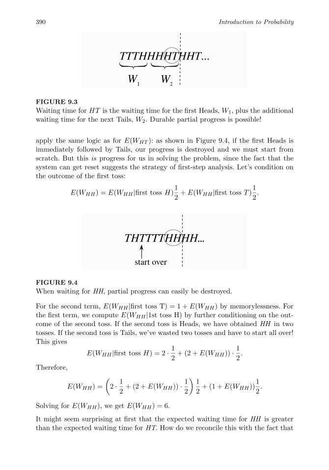
390 Introduction to Probability
TTTHHHHTHHT...
W1 W2
FIGURE 9.3
Waiting time for HT is the waiting time for the first Heads, W1
, plus the additionalwaiting time for the next Tails, W
2
. Durable partial progress is possible!
apply the same logic as for E(WHT ): as shown in Figure 9.4, if the first Heads isimmediately followed by Tails, our progress is destroyed and we must start fromscratch. But this is progress for us in solving the problem, since the fact that thesystem can get reset suggests the strategy of first-step analysis. Let’s condition onthe outcome of the first toss:
E(WHH) = E(WHH |first toss H)1
2+ E(WHH |first toss T )1
2.
THTTTTHHHH...
start over
FIGURE 9.4
When waiting for HH, partial progress can easily be destroyed.
For the second term, E(WHH |first toss T) = 1 + E(WHH) by memorylessness. Forthe first term, we compute E(WHH |1st toss H) by further conditioning on the out-come of the second toss. If the second toss is Heads, we have obtained HH in twotosses. If the second toss is Tails, we’ve wasted two tosses and have to start all over!This gives
E(WHH |first toss H) = 2 · 12+ (2 + E(WHH)) · 1
2.
Therefore,
E(WHH) =
✓2 · 1
2+ (2 + E(WHH)) · 1
2
◆1
2+ (1 + E(WHH))
1
2.
Solving for E(WHH), we get E(WHH) = 6.
It might seem surprising at first that the expected waiting time for HH is greaterthan the expected waiting time for HT. How do we reconcile this with the fact that

Conditional expectation 391
in two tosses of the coin, HH and HT both have a 1/4 chance of appearing? Whyaren’t the average waiting times the same by symmetry?
As we solved this problem, we in fact noticed an important asymmetry. Whenwaiting for HT, once we get the first Heads, we’ve achieved partial progress thatcannot be destroyed: if the Heads is followed by another Heads, we’re in the sameposition as before, and if the Heads is followed by a Tails, we’re done. By contrast,when waiting for HH, even after getting the first Heads, we could be sent back tosquare one if the Heads is followed by a Tails. This suggests the average waitingtime for HH should be longer. Symmetry implies that the average waiting time forHH is the same as that for TT, and that for HT is the same as that for TH, but itdoes not imply that the average waiting times for HH and HT are the same.
More intuition into what’s going on can be obtained by considering a long stringof coin flips, as in Figure 9.5. We notice right away that appearances of HH canoverlap, while appearances of HT must be disjoint. Since there are the same averagenumber of HH s and HT s, but HH s clump together while HT s do not, the spacingbetween successive strings of HH s must be greater to compensate.
HHTHHTTHHHHTHTHTTHTT
HHTHHTTHHHHTHTHTTHTT
FIGURE 9.5
Clumping. (a) Appearances of HH can overlap. (b) Appearances of HT must bedisjoint.
Related problems occur in information theory when compressing a message, and ingenetics when looking for recurring patterns (called motifs) in DNA sequences. ⇤Our final example in this section uses wishful thinking for both probabilities andexpectations to study a question about a random walk.
Example 9.1.10 (Random walk on the integers). An immortal drunk man wandersaround randomly on the integers. He starts at the origin, and at each step he moves1 unit to the right or 1 unit to the left, with equal probabilities, independently of allhis previous steps. Let b be a googolplex (this is 10g, where g = 10100 is a googol).
(a) Find a simple expression for the probability that the immortal drunk visits bbefore returning to the origin for the first time.
(b) Find the expected number of times that the immortal drunk visits b beforereturning to the origin for the first time.
Solution:
(a) Let B be the event that the drunk man visits b before returning to the origin

392 Introduction to Probability
for the first time and let L be the event that his first move is to the left. ThenP (B|L) = 0 since any path from �1 to b must pass through 0. For P (B|Lc), we areexactly in the setting of the gambler’s ruin problem, where player A starts with $1,player B starts with $(b�1), and the rounds are fair. Applying that result, we have
P (B) = P (B|L)P (L) + P (B|Lc)P (Lc) =1
b· 12=
1
2b.
(b) Let N be the number of visits to b before returning to the origin for the firsttime, and let p = 1/(2b) be the probability found in (a). Then
E(N) = E(N |N = 0)P (N = 0) + E(N |N � 1)P (N � 1) = pE(N |N � 1).
The conditional distribution of N given N � 1 is FS(p): given that the man reachesb, by symmetry there is probability p of returning to the origin before visiting b again(call this “success”) and probability 1 � p of returning to b again before returningto the origin (call this “failure”). Note that the trials are independent since thesituation is the same each time he is at b, independent of the past history. ThusE(N |N � 1) = 1/p, and
E(N) = pE(N |N � 1) = p · 1p= 1.
Surprisingly, the result doesn’t depend on the value of b, and our proof didn’t requireknowing the value of p. ⇤
9.2 Conditional expectation given an r.v.
In this section we introduce conditional expectation given a random variable. Thatis, we want to understand what it means to write E(Y |X) for an r.v. X. We will seethat E(Y |X) is a random variable that is, in a certain sense, our best prediction ofY , assuming we get to know X.
The key to understanding E(Y |X) is first to understand E(Y |X = x). Since X = xis an event, E(Y |X = x) is just the conditional expectation of Y given this event,and it can be computed using the conditional distribution of Y given X = x.
If Y is discrete, we use the conditional PMF P (Y = y|X = x) in place of theunconditional PMF P (Y = y):
E(Y |X = x) =X
y
yP (Y = y|X = x).
Analogously, if Y is continuous, we use the conditional PDF fY |X(y|x) in place ofthe unconditional PDF:
E(Y |X = x) =
Z 1
�1yfY |X(y|x)dy.

Conditional expectation 393
Notice that because we sum or integrate over y, E(Y |X = x) is a function of xonly. We can give this function a name, like g: let g(x) = E(Y |X = x). We defineE(Y |X) as the random variable obtained by finding the form of the function g(x),then plugging in X for x.
Definition 9.2.1 (Conditional expectation given an r.v.). Let g(x) = E(Y |X = x).Then the conditional expectation of Y given X, denoted E(Y |X), is defined to be therandom variable g(X). In other words, if after doing the experiment X crystallizesinto x, then E(Y |X) crystallizes into g(x).
h 9.2.2. The notation in this definition sometimes causes confusion. It does notsay “g(x) = E(Y |X = x), so g(X) = E(Y |X = X), which equals E(Y ) becauseX = X is always true”. Rather, we should first compute the function g(x), thenplug in X for x. For example, if g(x) = x2, then g(X) = X2. A similar biohazard ish 5.3.2, about the meaning of F (X) in the Universality of the Uniform.
h 9.2.3. By definition, E(Y |X) is a function of X, so it is a random variable.Thus it makes sense to compute quantities like E(E(Y |X)) and Var(E(Y |X)), themean and variance of the r.v. E(Y |X). It is easy to be ensnared by category errorswhen working with conditional expectation, so we should always keep in mind thatconditional expectations of the form E(Y |A) are numbers, while those of the formE(Y |X) are random variables.
Here are some quick examples of how to calculate conditional expectation. In bothexamples, we don’t need to do a sum or integral to get E(Y |X = x) because a moredirect approach is available.
Example 9.2.4. Suppose we have a stick of length 1 and break the stick at apoint X chosen uniformly at random. Given that X = x, we then choose anotherbreakpoint Y uniformly on the interval [0, x]. Find E(Y |X), and its mean andvariance.
Solution:
From the description of the experiment, X ⇠ Unif(0, 1) and Y |X = x ⇠ Unif(0, x).Then E(Y |X = x) = x/2, so by plugging in X for x, we have
E(Y |X) = X/2.
The expected value of E(Y |X) is
E(E(Y |X)) = E(X/2) = 1/4.
(We will show in the next section that a general property of conditional expectationis that E(E(Y |X)) = E(Y ), so it also follows that E(Y ) = 1/4.) The variance ofE(Y |X) is
Var(E(Y |X)) = Var(X/2) = 1/48.
⇤

394 Introduction to Probability
Example 9.2.5. For X,Yi.i.d.⇠ Expo(�), find E(max(X,Y )|min(X,Y )).
Solution:
Let M = max(X,Y ) and L = min(X,Y ). By the memoryless property, M � L isindependent of L, and M � L ⇠ Expo(�) (see Example 7.3.6). Therefore
E(M |L = l) = E(L|L = l) + E(M � L|L = l) = l + E(M � L) = l +1
�,
and E(M |L) = L+ 1
� . ⇤
9.3 Properties of conditional expectation
Conditional expectation has some very useful properties, that often allow us to solveproblems without having to go all the way back to the definition.
• Dropping what’s independent: If X and Y are independent, then E(Y |X) = E(Y ).
• Taking out what’s known: For any function h, E(h(X)Y |X) = h(X)E(Y |X).
• Linearity: E(Y1
+ Y2
|X) = E(Y1
|X) +E(Y2
|X), and E(cY |X) = cE(Y |X) for c aconstant (the latter is a special case of taking out what’s known).
• Adam’s law: E(E(Y |X)) = E(Y ).
• Projection interpretation: The r.v. Y �E(Y |X), which is called the residual fromusing X to predict Y , is uncorrelated with h(X) for any function h.
Let’s discuss each property individually.
Theorem 9.3.1 (Dropping what’s independent). If X and Y are independent, thenE(Y |X) = E(Y ).
This is true because independence implies E(Y |X = x) = E(Y ) for all x, henceE(Y |X) = E(Y ). Intuitively, if X provides no information about Y , then our bestguess for Y , even if we get to knowX, is still the unconditional mean E(Y ). However,the converse is false: a counterexample is given in Example 9.3.3 below.
Theorem 9.3.2 (Taking out what’s known). For any function h,
E(h(X)Y |X) = h(X)E(Y |X).
Intuitively, when we take expectations given X, we are treating X as if it hascrystallized into a known constant. Then any function of X, say h(X), also acts likea known constant while we are conditioning on X. Taking out what’s known is theconditional version of the unconditional fact that E(cY ) = cE(Y ). The di↵erence isthat E(cY ) = cE(Y ) asserts that two numbers are equal, while taking out what’sknown asserts that two random variables are equal.

Conditional expectation 395
Example 9.3.3. Let Z ⇠ N (0, 1) and Y = Z2. Find E(Y |Z) and E(Z|Y ).
Solution:
Since Y is a function of Z, E(Y |Z) = E(Z2|Z) = Z2 by taking out what’s known.To get E(Z|Y ), notice that conditional on Y = y, Z equals
py or �p
y with equalprobabilities by the symmetry of the standard Normal, so E(Z|Y = y) = 0 andE(Z|Y ) = 0.
In this case, although Y provides a lot of information about Z, narrowing down thepossible values of Z to just two values, Y only tells us about the magnitude of Zand not its sign. For this reason, E(Z|Y ) = E(Z) despite the dependence betweenZ and Y . This example illustrates that the converse of Theorem 9.3.1 is false. ⇤
Theorem 9.3.4 (Linearity). E(Y1
+ Y2
|X) = E(Y1
|X) + E(Y2
|X).
This result is the conditional version of the unconditional fact that E(Y1
+ Y2
) =E(Y
1
) + E(Y2
), and is true since conditional probabilities are probabilities.
h 9.3.5. It is incorrect to write “E(Y |X1
+X2
) = E(Y |X1
) +E(Y |X2
)”; linearityapplies on the left side of the conditioning bar, not on the right side!
Example 9.3.6. Let X1
, . . . , Xn be i.i.d., and Sn = X1
+ · · ·+Xn. Find E(X1
|Sn).
Solution:
By symmetry,
E(X1
|Sn) = E(X2
|Sn) = · · · = E(Xn|Sn),
and by linearity,
E(X1
|Sn) + · · ·+ E(Xn|Sn) = E(Sn|Sn) = Sn.
Therefore,
E(X1
|Sn) = Sn/n = Xn,
the sample mean of theXj ’s. This is an intuitive result: if we have 2 i.i.d. r.v.sX1
, X2
and learn that X1
+X2
= 10, it makes sense to guess that X1
is 5 (accounting forhalf of the total). Similarly, if we have n i.i.d. r.v.s and get to know their sum, ourbest guess for any one of them is the sample mean. ⇤
The next theorem connects conditional expectation to unconditional expectation.It goes by many names, including the law of total expectation, the law of iteratedexpectation (which has a terrible acronym for something glowing with truth), andthe tower property. We call it Adam’s law because it is used so frequently that itdeserves a pithy name, and since it is often used in conjunction with another lawwe’ll encounter soon, which has a complementary name.
Theorem 9.3.7 (Adam’s law). For any r.v.s X and Y ,
E(E(Y |X)) = E(Y ).

396 Introduction to Probability
Proof. We present the proof in the case where X and Y are both discrete (theproofs for other cases are analogous). Let E(Y |X) = g(X). We proceed by applyingLOTUS, expanding the definition of g(x) to get a double sum, and then swappingthe order of summation:
E(g(X)) =X
x
g(x)P (X = x)
=X
x
X
y
yP (Y = y|X = x)
!P (X = x)
=X
x
X
y
yP (X = x)P (Y = y|X = x)
=X
y
yX
x
P (X = x, Y = y)
=X
y
yP (Y = y) = E(Y ).
⌅
Adam’s law is a more compact, more general version of the law of total expectation(Theorem 9.1.5). For X discrete, the statements
E(Y ) =X
x
E(Y |X = x)P (X = x)
and
E(Y ) = E(E(Y |X))
mean the same thing, since if we let E(Y |X = x) = g(x), then
E(E(Y |X)) = E(g(X)) =X
x
g(x)P (X = x) =X
x
E(Y |X = x)P (X = x).
But the Adam’s law expression is shorter and applies just as well in the continuouscase.
Armed with Adam’s law, we have a powerful strategy for finding an expectationE(Y ), by conditioning on an r.v. X that we wish we knew. First obtain E(Y |X) bytreating X as known, and then take the expectation of E(Y |X). We will see variousexamples of this later in the chapter.
Just as there are forms of Bayes’ rule and LOTP with extra conditioning, as dis-cussed in Chapter 2, there is a version of Adam’s law with extra conditioning.
Theorem 9.3.8 (Adam’s law with extra conditioning). For any r.v.s X,Y, Z, wehave
E(E(Y |X,Z)|Z) = E(Y |Z).

Conditional expectation 397
The above equation is Adam’s law, except with extra conditioning on Z insertedeverywhere. It is true because conditional probabilities are probabilities. So weare free to use Adam’s law to help us find both unconditional expectations andconditional expectations.
Using Adam’s law, we can also prove the last item on our list of properties ofconditional expectation.
Theorem 9.3.9 (Projection interpretation). For any function h, the r.v. Y �E(Y |X) is uncorrelated with h(X). Equivalently,
E((Y � E(Y |X))h(X)) = 0.
(This is equivalent since E(Y � E(Y |X)) = 0, by linearity and Adam’s law.)
Proof. We have
E((Y � E(Y |X))h(X)) = E(h(X)Y )� E(h(X)E(Y |X))
= E(h(X)Y )� E(E(h(X)Y |X))
by Theorem 9.3.2 (here we’re “putting back what’s known” into the inner expecta-tion). By Adam’s law, the second term is equal to E(h(X)Y ). ⌅
Y
E(Y | X)
Y – E(Y | X)
FIGURE 9.6
The conditional expectation E(Y |X) is the projection of Y onto the space of allfunctions of X, shown here as a plane. The residual Y � E(Y |X) is orthogonal tothe plane: it’s perpendicular to (uncorrelated with) any function of X.
From a geometric perspective, we can visualize Theorem 9.3.9 as in Figure 9.6. In acertain sense (described below), E(Y |X) is the function of X that is closest to Y ;we say that E(Y |X) is the projection of Y into the space of all functions of X. The“line” from Y to E(Y |X) in the figure is orthogonal (perpendicular) to the “plane”,since any other route from Y to E(Y |X) would be longer. This orthogonality turnsout to be the geometric interpretation of Theorem 9.3.9.
The details of this perspective are given in the next section, which is starred sinceit requires knowledge of linear algebra. But even without delving into the linearalgebra, the projection picture gives some useful intuition. As mentioned earlier, we

398 Introduction to Probability
can think of E(Y |X) as a prediction for Y based on X. This is an extremely com-mon problem in statistics: predict or estimate the future observations or unknownparameters based on data. The projection interpretation of conditional expectationimplies that E(Y |X) is the best predictor of Y based on X, in the sense that it isthe function of X with the lowest mean squared error (expected squared di↵erencebetween Y and the prediction of Y ).
Example 9.3.10 (Linear regression). An extremely widely used method for dataanalysis in statistics is linear regression. In its most basic form, the linear regressionmodel uses a single explanatory variable X to predict a response variable Y , and itassumes that the conditional expectation of Y is linear in X:
E(Y |X) = a+ bX.
(a) Show that an equivalent way to express this is to write
Y = a+ bX + ✏,
where ✏ is an r.v. (called the error) with E(✏|X) = 0.
(b) Solve for the constants a and b in terms of E(X), E(Y ), Cov(X,Y ), and Var(X).
Solution:
(a) Let Y = a+ bX + ✏, with E(✏|X) = 0. Then by linearity,
E(Y |X) = E(a|X) + E(bX|X) + E(✏|X) = a+ bX.
Conversely, suppose that E(Y |X) = a+ bX, and define
✏ = Y � (a+ bX).
Then Y = a+ bX + ✏, with
E(✏|X) = E(Y |X)� E(a+ bX|X) = E(Y |X)� (a+ bX) = 0.
(b) First, by Adam’s law, taking the expectation of both sides gives
E(Y ) = a+ bE(X).
Note that ✏ has mean 0 and X and ✏ are uncorrelated, since
E(✏) = E(E(✏|X)) = E(0) = 0
andE(✏X) = E(E(✏X|X)) = E(XE(✏|X)) = E(0) = 0.
Taking the covariance with X of both sides in Y = a+ bX + ✏, we have
Cov(X,Y ) = Cov(X, a) + bCov(X,X) + Cov(X, ✏) = bVar(X).

Conditional expectation 399
Thus,
b =Cov(X,Y )
Var(X),
a = E(Y )� bE(X) = E(Y )� Cov(X,Y )
Var(X)· E(X).
⇤
9.4 *Geometric interpretation of conditional expectation
This section explains in more detail the geometric perspective shown in Figure 9.6,using some concepts from linear algebra. Consider the vector space consisting of allrandom variables on a certain probability space, such that the random variables eachhave zero mean and finite variance. (To apply the concepts of this section to r.v.sthat don’t have zero mean, we can center them first by subtracting their means.)Each vector or point in the space is a random variable (here we are using “vector”in the linear algebra sense, not in the sense of a random vector from Chapter 7).Define the inner product of two r.v.s U and V to be
hU, V i = Cov(U, V ) = E(UV ).
(For this definition to satisfy the axioms for an inner product, we need the conventionthat two r.v.s are considered the same if they are equal with probability 1.)
With this definition, two r.v.s are uncorrelated if and only if they have an innerproduct of 0, which means they are orthogonal in the vector space. The squaredlength of an r.v. X is
||X||2 = hX,Xi = Var(X) = EX2,
so the length of an r.v. is its standard deviation. The squared distance betweentwo r.v.s U and V is E(U � V )2, and the cosine of the angle between them is thecorrelation between them.
The random variables that can be expressed as functions of X form a subspace ofthe vector space. In Figure 9.6, the subspace of random variables of the form h(X)is represented by a plane. To get E(Y |X), we project Y onto the plane. Then theresidual Y � E(Y |X) is orthogonal to h(X) for all functions h, and E(Y |X) is thefunction of X that best predicts Y , where “best” here means that the mean squarederror E(Y � g(X))2 is minimized by choosing g(X) = E(Y |X).
The projection interpretation is a helpful way to think about many of the propertiesof conditional expectation. For example, if Y = h(X) is a function ofX, then Y itself

400 Introduction to Probability
is already in the “plane”, so it is its own projection; this explains why E(h(X)|X) =h(X). Also, we can think of unconditional expectation as a projection too: E(Y ) =E(Y |0) is the projection of Y onto the space of all constants (and indeed, E(Y ) isthe constant c that minimizes E(Y � c)2, as we proved in Theorem 6.1.4).
We can now also give a geometric interpretation for Adam’s law: E(Y ) says toproject Y in one step to the space of all constants; E(E(Y |X)) says to do it in twosteps, by first projecting onto the “plane” and then projecting E(Y |X) onto thespace of all constants, which is a line within that “plane”. Adam’s law says that theone-step and two-step methods yield the same result.
9.5 Conditional variance
Once we’ve defined conditional expectation given an r.v., we have a natural way todefine conditional variance given an r.v.: replace all instances of E(·) in the definitionof unconditional variance with E(·|X).
Definition 9.5.1 (Conditional variance). The conditional variance of Y given Xis
Var(Y |X) = E((Y � E(Y |X))2|X).
This is equivalent to
Var(Y |X) = E(Y 2|X)� (E(Y |X))2.
h 9.5.2. Like E(Y |X), Var(Y |X) is a random variable, and it is a function of X.
Since conditional variance is defined in terms of conditional expectations, we canuse results about conditional expectation to help us calculate conditional variance.Here’s an example.
Example 9.5.3. Let Z ⇠ N (0, 1) and Y = Z2. Find Var(Y |Z) and Var(Z|Y ).
Solution:
Without any calculations we can see that Var(Y |Z) = 0: conditional on Z, Y isa known constant, and the variance of a constant is 0. By the same reasoning,Var(h(Z)|Z) = 0 for any function h.
To get Var(Z|Y ), apply the definition:
Var(Z|Z2) = E(Z2|Z2)� (E(Z|Z2))2.
The first term equals Z2. The second term equals 0 by symmetry, as we found inExample 9.3.3. Thus Var(Z|Z2) = Z2, which we can write as Var(Z|Y ) = Y . ⇤

Conditional expectation 401
We learned in the previous section that Adam’s law relates conditional expectationto unconditional expectation. A companion result for Adam’s law is Eve’s law, whichrelates conditional variance to unconditional variance.
Theorem 9.5.4 (Eve’s law). For any r.v.s X and Y ,
Var(Y ) = E(Var(Y |X)) + Var(E(Y |X)).
The ordering of E’s and Var’s on the right-hand side spells EVVE, whence thename Eve’s law. Eve’s law is also known as the law of total variance or the variancedecomposition formula.
Proof. Let g(X) = E(Y |X). By Adam’s law, E(g(X)) = E(Y ). Then
E(Var(Y |X)) = E(E(Y 2|X)� g(X)2) = E(Y 2)� E(g(X)2),
Var(E(Y |X)) = E(g(X)2)� (Eg(X))2 = E(g(X)2)� (EY )2.
Adding these equations, we have Eve’s law. ⌅
To visualize Eve’s law, imagine a population where each person has a value of Xand a value of Y . We can divide this population into subpopulations, one for eachpossible value of X. For example, if X represents age and Y represents height, wecan group people based on age. Then there are two sources contributing to thevariation in people’s heights in the overall population. First, within each age group,people have di↵erent heights. The average amount of variation in height within eachage group is the within-group variation, E(Var(Y |X)). Second, across age groups,the average heights are di↵erent. The variance of average heights across age groupsis the between-group variation, Var(E(Y |X)). Eve’s law says that to get the totalvariance of Y , we simply add these two sources of variation.
Figure 9.7 illustrates Eve’s law in the simple case where we have three age groups.The average amount of scatter within each of the groups X = 1, X = 2, andX = 3 is the within-group variation, E(Var(Y |X)). The variance of the groupmeans E(Y |X = 1), E(Y |X = 2), and E(Y |X = 3) is the between-group variation,Var(E(Y |X)).
X = 1 X = 2 X = 3
FIGURE 9.7
Eve’s law says that total variance is the sum of within-group and between-groupvariation.

402 Introduction to Probability
Another way to think about Eve’s law is in terms of prediction. If we wanted topredict someone’s height based on their age alone, the ideal scenario would be if ev-eryone within an age group had exactly the same height, while di↵erent age groupshad di↵erent heights. Then, given someone’s age, we would be able to predict theirheight perfectly. In other words, the ideal scenario for prediction is no within-groupvariation in height, since the within-group variation cannot be explained by age dif-ferences. For this reason, within-group variation is also called unexplained variation,and between-group variation is also called explained variation. Eve’s law says thatthe total variance of Y is the sum of unexplained and explained variation.
h 9.5.5. Let Y be an r.v. and A be an event. It is wrong to say “Var(Y ) =Var(Y |A)P (A) + Var(Y |Ac)P (Ac)”, even though this looks analogous to the lawof total expectation. Rather, we should use Eve’s law if we want to condition onwhether or not A occurred: letting I be the indicator of A,
Var(Y ) = E(Var(Y |I)) + Var(E(Y |I)).
To see how this expression relates to the “wrong expression”, let
p = P (A), q = P (Ac), a = E(Y |A), b = E(Y |Ac), v = Var(Y |A), w = Var(Y |Ac).
Then E(Y |I) is a with probability p and b with probability q, and Var(Y |I) is vwith probability p and w with probability q. So
E(Var(Y |I)) = vp+ wq = Var(Y |A)P (A) + Var(Y |Ac)P (Ac),
which is exactly the “wrong expression”, and Var(Y ) consists of this plus the term
Var(E(Y |I)) = a2p+ b2q � (ap+ bq)2.
It is crucial to account for both within-group and between-group variation.
9.6 Adam and Eve examples
We conclude this chapter with several examples showing how Adam’s law and Eve’slaw allow us to find the mean and variance of complicated r.v.s, especially in situ-ations that involve multiple levels of randomness.
In our first example, the r.v. of interest is the sum of a random number of randomvariables. There are thus two levels of randomness: first, each term in the sumis a random variable; second, the number of terms in the sum is also a randomvariable.
Example 9.6.1 (Random sum). A store receives N customers in a day, where Nis an r.v. with finite mean and variance. Let Xj be the amount spent by the jth

Conditional expectation 403
customer at the store. Assume that each Xj has mean µ and variance �2, and thatN and all the Xj are independent of one another. Find the mean and variance of
the random sum X =PN
j=1
Xj , which is the store’s total revenue in a day, in terms
of µ, �2, E(N), and Var(N).
Solution:
Since X is a sum, our first impulse might be to claim “E(X) = Nµ by linearity”.Alas, this would be a category error, since E(X) is a number and Nµ is a randomvariable. The key is that X is not merely a sum, but a random sum; the number ofterms we are adding up is itself random, whereas linearity applies to sums with afixed number of terms.
Yet this category error actually suggests the correct strategy: if only we were allowedto treat N as a constant, then linearity would apply. So let’s condition on N ! Bylinearity of conditional expectation,
E(X|N) = E(NX
j=1
Xj |N) =NX
j=1
E(Xj |N) =NX
j=1
E(Xj) = Nµ.
We used the independence of the Xj and N to assert E(Xj |N) = E(Xj) for allj. Note that the statement “E(X|N) = Nµ” is not a category error because bothsides of the equality are r.v.s that are functions of N . Finally, by Adam’s law,
E(X) = E(E(X|N)) = E(Nµ) = µE(N).
This is a pleasing result: the average total revenue is the average amount spent percustomer, multiplied by the average number of customers.
For Var(X), we again condition on N to get Var(X|N):
Var(X|N) = Var(NX
j=1
Xj |N) =NX
j=1
Var(Xj |N) =NX
j=1
Var(Xj) = N�2.
Eve’s law then tells us how to obtain the unconditional variance of X:
Var(X) = E(Var(X|N)) + Var(E(X|N))
= E(N�2) + Var(Nµ)
= �2E(N) + µ2Var(N).
⇤
In the next example, two levels of randomness arise because our experiment takesplace in two stages. We sample a city from a group of cities, then sample citizenswithin the city. This is an example of a multilevel model.

404 Introduction to Probability
Example 9.6.2 (Random sample from a random city). To study the prevalenceof a disease in several cities of interest within a certain county, we pick a city atrandom, then pick a random sample of n people from that city. This is a form of awidely used survey technique known as cluster sampling.
Let Q be the proportion of diseased people in the chosen city, and let X be thenumber of diseased people in the sample. As illustrated in Figure 9.8 (where whitedots represent healthy individuals and black dots represent diseased individuals),di↵erent cities may have very di↵erent prevalences. Since each city has its owndisease prevalence, Q is a random variable. Suppose that Q ⇠ Unif(0, 1). Alsoassume that conditional on Q, each individual in the sample independently hasprobability Q of having the disease; this is true if we sample with replacement fromthe chosen city, and is approximately true if we sample without replacement butthe population size is large. Find E(X) and Var(X).
FIGURE 9.8
A certain oval-shaped county has 4 cities. Each city has healthy people (representedas white dots) and diseased people (represented as black dots). A random city ischosen, and then a random sample of n people is chosen from within that city.There are two components to the variability in the number of diseased people inthe sample: variation due to di↵erent cities having di↵erent disease prevalence, andvariation due to the randomness of the sample within the chosen city.
Solution:
With our assumptions, X|Q ⇠ Bin(n,Q); this notation says that conditional onknowing the disease prevalence in the chosen city, we can treat Q as a constant,and each sampled individual is an independent Bernoulli trial with probability Q ofsuccess. Using the mean and variance of the Binomial distribution, E(X|Q) = nQand Var(X|Q) = nQ(1 � Q). Furthermore, using the moments of the standardUniform distribution, E(Q) = 1/2, E(Q2) = 1/3, and Var(Q) = 1/12. Now we canapply Adam’s law and Eve’s law to get the unconditional mean and variance of X:
E(X) = E(E(X|Q)) = E(nQ) =n
2,

Conditional expectation 405
Var(X) = E(Var(X|Q)) + Var(E(X|Q))
= E(nQ(1�Q)) + Var(nQ)
= nE(Q)� nE(Q2) + n2Var(Q)
=n
6+
n2
12.
Note that the structure of this problem is identical to that in the story of Bayes’billiards. Therefore, we actually know the distribution of X, not just its mean andvariance:X is Discrete Uniform on {0, 1, 2, . . . , n}. But the Adam-and-Eve approachcan be applied when Q has a more complicated distribution, or with more levels inthe multilevel model, whether or not it is feasible to work out the distribution ofX. For example, we could have people within cities within counties within stateswithin countries. ⇤Last but not least, we revisit Story 8.4.5, the Gamma-Poisson problem from theprevious chapter.
Example 9.6.3 (Gamma-Poisson revisited). Recall that Fred decided to find outabout the rate of Blotchville’s Poisson process of buses by waiting at the bus stopfor t hours and counting the number of buses Y . He then used the data to updatehis prior distribution � ⇠ Gamma(r
0
, b0
). Thus, Fred was using the two-level model
� ⇠ Gamma(r0
, b0
)
Y |� ⇠ Pois(�t).
We found that under Fred’s model, the marginal distribution of Y is NegativeBinomial with parameters r = r
0
and p = b0
/(b0
+ t). By the mean and variance ofthe Negative Binomial distribution, we have
E(Y ) =rq
p=
r0
t
b0
,
Var(Y ) =rq
p2=
r0
t(b0
+ t)
b20
.
Let’s independently verify this with Adam’s law and Eve’s law. Using resultsabout the Poisson distribution, the conditional mean and variance of Y given �are E(Y |�) = Var(Y |�) = �t. Using results about the Gamma distribution, themarginal mean and variance of � are E(�) = r
0
/b0
and Var(�) = r0
/b20
. For Adamand Eve, this is all that is required:
E(Y ) = E(E(Y |�)) = E(�t) =r0
t
b0
,
Var(Y ) = E(Var(Y |�)) + Var(E(Y |�))= E(�t) + Var(�t)
=r0
t
b0
+r0
t2
b20
=r0
t(b0
+ t)
b20
,
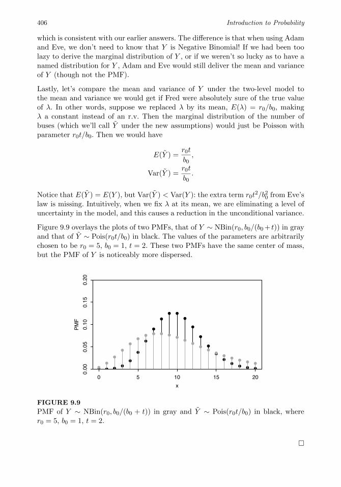
406 Introduction to Probability
which is consistent with our earlier answers. The di↵erence is that when using Adamand Eve, we don’t need to know that Y is Negative Binomial! If we had been toolazy to derive the marginal distribution of Y , or if we weren’t so lucky as to have anamed distribution for Y , Adam and Eve would still deliver the mean and varianceof Y (though not the PMF).
Lastly, let’s compare the mean and variance of Y under the two-level model tothe mean and variance we would get if Fred were absolutely sure of the true valueof �. In other words, suppose we replaced � by its mean, E(�) = r
0
/b0
, making� a constant instead of an r.v. Then the marginal distribution of the number ofbuses (which we’ll call Y under the new assumptions) would just be Poisson withparameter r
0
t/b0
. Then we would have
E(Y ) =r0
t
b0
,
Var(Y ) =r0
t
b0
.
Notice that E(Y ) = E(Y ), but Var(Y ) < Var(Y ): the extra term r0
t2/b20
from Eve’slaw is missing. Intuitively, when we fix � at its mean, we are eliminating a level ofuncertainty in the model, and this causes a reduction in the unconditional variance.
Figure 9.9 overlays the plots of two PMFs, that of Y ⇠ NBin(r0
, b0
/(b0
+ t)) in grayand that of Y ⇠ Pois(r
0
t/b0
) in black. The values of the parameters are arbitrarilychosen to be r
0
= 5, b0
= 1, t = 2. These two PMFs have the same center of mass,but the PMF of Y is noticeably more dispersed.
0 5 10 15 20
0.00
0.05
0.10
0.15
0.20
x
PMF
● ● ●●
●
●
●
●
●
● ●
●
●
●
●
●
●●
● ● ●●
●
●
●
●
●●
● ● ●●
●●
●●
●●
●●
● ●
FIGURE 9.9
PMF of Y ⇠ NBin(r0
, b0
/(b0
+ t)) in gray and Y ⇠ Pois(r0
t/b0
) in black, wherer0
= 5, b0
= 1, t = 2.
⇤
Conditional expectation 407
9.7 Recap
To calculate an unconditional expectation, we can divide up the sample space anduse the law of total expectation
E(Y ) =nX
i=1
E(Y |Ai)P (Ai),
but we must be careful not to destroy information in subsequent steps (such as byforgetting in the midst of a long calculation to condition on something that needs tobe conditioned on). In problems with a recursive structure, we can also use first-stepanalysis for expectations.
The conditional expectation E(Y |X) and conditional variance Var(Y |X) are ran-dom variables that are functions of X; they are obtained by treating X as if itwere a known constant. If X and Y are independent, then E(Y |X) = E(Y ) andVar(Y |X) = Var(Y ). Conditional expectation has the properties
E(h(X)Y |X) = h(X)E(Y |X)
E(Y1
+ Y2
|X) = E(Y1
|X) + E(Y2
|X),
analogous to the properties E(cY ) = cE(Y ) and E(Y1
+ Y2
) = E(Y1
) + E(Y2
) forunconditional expectation. The conditional expectation E(Y |X) is also the randomvariable that makes the residual Y �E(Y |X) uncorrelated with any function of X,which means we can interpret it geometrically as a projection.
Finally, Adam’s law and Eve’s law,
E(Y ) = E(E(Y |X))
Var(Y ) = E(Var(Y |X)) + Var(E(Y |X)),
often help us calculate E(Y ) and Var(Y ) in problems that feature multiple formsor levels of randomness.
Figure 9.10 illustrates how the number E(Y |X = x) connects with the r.v. E(Y |X),whose expectation is E(Y ) by Adam’s law. Additionally, it shows how the ingredi-ents in Eve’s law are formed and come together to give a useful decomposition ofVar(Y ) in terms of quantities that condition on X.

408 Introduction to Probability
X,YE(Y | X = x)
(function of x)
condition on r.v.
random variables events numbers
X = xgenerate
Var(Y) = E(Var(Y | X)) + Var(E(Y | X))(Eve's law)
E(Y | X)(function of X)
E(E(Y | X)) = E(Y) (Adam's law)
x
−3−2
−10
12
3y
−3
−2
−1
0
1
2
3
0.00
0.05
0.10
0.15
0.20
joint CDF F(x,y)joint PMF P(X = x, Y = y)
joint PDF f(x,y)joint MGF M(s,t)
joint distributions
Var(Y | X)(function of X)
condition on event
E(Var(Y | X))(within group variation)
Var(E(Y | X))(between group variation)
+
variance
expectation
expectation
What can happen?
FIGURE 9.10
We often observe an r.v. X and want to predict another r.v. Y based on the infor-mation about X. If we observe that X = x, then we can condition on that eventand use E(Y |X = x) as our prediction. The conditional expectation E(Y |X) is ther.v. that takes the value E(Y |X = x) when X = x. Adam’s law lets us computethe unconditional expectation E(Y ) by starting with the conditional expectationE(Y |X). Similarly, Eve’s law lets us compute Var(Y ) in terms of quantities thatcondition on X.
9.8 R
Mystery prize simulation
We can use simulation to show that in Example 9.1.7, the example of bidding on amystery prize with unknown value, any bid will lead to a negative payout on average.First choose a bid b (we chose 0.6); then simulate a large number of hypotheticalmystery prizes and store them in v:
b <- 0.6

Conditional expectation 409
nsim <- 10^5
v <- runif(nsim)
The bid is accepted if b > (2/3)*v. To get the average profit conditional on anaccepted bid, we use square brackets to keep only those values of v satisfying thecondition:
mean(v[b > (2/3)*v]) - b
This value is negative regardless of b, as you can check by experimenting withdi↵erent values of b.
Time until HH vs. HT
To verify the results of Example 9.1.9, we can start by generating a long sequenceof fair coin tosses. This is done with the sample command. We use paste with thecollapse="" argument to turn these tosses into a single string ofH’s and T ’s:
paste(sample(c("H","T"),100,replace=TRUE),collapse="")
A sequence of length 100 is enough to virtually guarantee that both HH and HTwill have appeared at least once.
To determine how many tosses are required on average to see HH and HT, weneed to generate many sequences of coin tosses. For this, we use our familiar friendreplicate:
r <- replicate(10^3,paste(sample(c("H","T"),100,replace=T),collapse=""))
Now r contains a thousand sequences of coin tosses, each of length 100. To find thefirst appearance of HH in each of these sequences, it is easiest to use the str_locatecommand, located in the stringr package. After you’ve installed and loaded thepackage,
t <- str_locate(r,"HH")
creates a two-column table t, whose columns contain the starting and ending posi-tions of the first appearance of HH in each sequence of coin tosses. (Use head(t) todisplay the first few rows of the table and get an idea of what your results look like.)What we want are the ending positions, given by the second column. In particular,we want the average value of the second column, which is an approximation of theaverage waiting time for HH :
mean(t[,2])
Is your answer around 6? Trying again with "HT" instead of "HH", is your answeraround 4?

410 Introduction to Probability
Linear regression
In Example 9.3.10, we derived formulas for the slope and intercept of a linear regres-sion model, which can be used to predict a response variable using an explanatoryvariable. Let’s try to apply these formulas to a simulated dataset:
x <- rnorm(100)
y <- 3 + 5*x + rnorm(100)
The vector x contains 100 realizations of the random variable X ⇠ N (0, 1), and thevector y contains 100 realizations of the random variable Y = a + bX + ✏ where✏ ⇠ N (0, 1). As we can see, the true values of a and b for this dataset are 3 and 5,respectively. We can visualize the data as a scatterplot with plot(x,y).
Now let’s see if we can get good estimates of the true a and b, using the formulasin Example 9.3.10:
b <- cov(x,y) / var(x)
a <- mean(y) - b*mean(x)
Here cov(x,y), var(x), and mean(x) provide the sample covariance, sample vari-ance, and sample mean, estimating the quantities Cov(X,Y ), Var(X), and E(X),respectively. (We have discussed sample mean and sample variance in detail in ear-lier chapters. Sample covariance is defined analogously, and is a natural way toestimate the true covariance.)
You should find that b is close to 5 and a is close to 3. These estimated values definethe line of best fit. The abline command lets us plot the line of best fit on top ofour scatterplot:
plot(x,y)
abline(a=a,b=b)
The first argument to abline is the intercept of the line, and the second argumentis the slope.
9.9 Exercises
Conditional expectation given an event
1. Fred wants to travel from Blotchville to Blissville, and is deciding between 3 options(involving di↵erent routes or di↵erent forms of transportation). The jth option wouldtake an average of µj hours, with a standard deviation of �j hours. Fred randomlychooses between the 3 options, with equal probabilities. Let T be how long it takes forhim to get from Blotchville to Blissville.
(a) Find E(T ). Is it simply (µ1
+ µ2
+ µ3
)/3, the average of the expectations?
(b) Find Var(T ). Is it simply (�2
1
+ �2
2
+ �2
3
)/3, the average of the variances?

Conditional expectation 411
2. While Fred is sleeping one night, X legitimate emails and Y spam emails are sent tohim. Suppose that X and Y are independent, with X ⇠ Pois(10) and Y ⇠ Pois(40).When he wakes up, he observes that he has 30 new emails in his inbox. Given thisinformation, what is the expected value of how many new legitimate emails he has?
3. A group of 21 women and 14 men are enrolled in a medical study. Each of them has acertain disease with probability p, independently. It is then found (through extremelyreliable testing) that exactly 5 of the people have the disease. Given this information,what is the expected number of women who have the disease? Again given this infor-mation, what is the expected number of women who have the disease?
4. A researcher studying crime is interested in how often people have gotten arrested. LetX ⇠ Pois(�) be the number of times that a random person got arrested in the last 10years. However, data from police records are being used for the researcher’s study, andpeople who were never arrested in the last 10 years do not appear in the records. Inother words, the police records have a selection bias: they only contain information onpeople who have been arrested in the last 10 years.
So averaging the numbers of arrests for people in the police records does not directly es-timate E(X); it makes more sense to think of the police records as giving us informationabout the conditional distribution of how many times a person was arrest, given thatthe person was arrested at least once in the last 10 years. The conditional distributionof X, given that X � 1, is called a truncated Poisson distribution (see Exercise 14 foranother example of this distribution).
(a) Find E(X|X � 1)
(b) Find Var(X|X � 1).
5. A fair 20-sided die is rolled repeatedly, until a gambler decides to stop. The gamblerpays $1 per roll, and receives the amount shown on the die when the gambler stops(e.g., if the die is rolled 7 times and the gambler decides to stop then, with an 18 as thevalue of the last roll, then the net payo↵ is $18� $7 = $11). Suppose the gambler usesthe following strategy: keep rolling until a value of m or greater is obtained, and thenstop (where m is a fixed integer between 1 and 20).
(a) What is the expected net payo↵?
Hint: The average of consecutive integers a, a+ 1, . . . , a+ n is the same as the averageof the first and last of these. See the math appendix for more information about series.
(b) Use R or other software to find the optimal value of m.
6. Let X ⇠ Expo(�). Find E(X|X < 1) in two di↵erent ways:
(a) by calculus, working with the conditional PDF of X given X < 1.
(b) without calculus, by expanding E(X) using the law of total expectation.
7. s� You get to choose between two envelopes, each of which contains a check for somepositive amount of money. Unlike in the two-envelope paradox, it is not given that oneenvelope contains twice as much money as the other envelope. Instead, assume that thetwo values were generated independently from some distribution on the positive realnumbers, with no information given about what that distribution is.
After picking an envelope, you can open it and see how much money is inside (call thisvalue x), and then you have the option of switching. As no information has been givenabout the distribution, it may seem impossible to have better than a 50% chance ofpicking the better envelope. Intuitively, we may want to switch if x is “small” and notswitch if x is “large”, but how do we define “small” and “large” in the grand scheme ofall possible distributions? [The last sentence was a rhetorical question.]
Consider the following strategy for deciding whether to switch. Generate a thresholdT ⇠ Expo(1), and switch envelopes if and only if the observed value x is less than the

412 Introduction to Probability
value of T . Show that this strategy succeeds in picking the envelope with more moneywith probability strictly greater than 1/2.
Hint: Let t be the value of T (generated by a random draw from the Expo(1) distribu-tion). First explain why the strategy works very well if t happens to be in between thetwo envelope values, and does no harm in any case (i.e., there is no case in which thestrategy succeeds with probability strictly less than 1/2).
8. There are two envelopes, each of which has a check for a Unif(0, 1) amount of money,measured in thousands of dollars. The amounts in the two envelopes are independent.You get to choose an envelope and open it, and then you can either keep that amountor switch to the other envelope and get whatever amount is in that envelope.
Suppose that you use the following strategy: choose an envelope and open it. If youobserve U , then stick with that envelope with probability U , and switch to the otherenvelope with probability 1� U .
(a) Find the probability that you get the larger of the two amounts.
(b) Find the expected value of what you will receive.
9. Suppose n people are bidding on a mystery prize that is up for auction. The bids are tobe submitted in secret, and the individual who submits the highest bid wins the prize.Each bidder receives an i.i.d. signal Xi, i = 1, . . . , n. The value of the prize, V , is definedto be the sum of the individual bidders’ signals:
V = X1
+ · · ·+Xn.
This is known in economics as the wallet game: we can imagine that the n people arebidding on the total amount of money in their wallets, and each person’s signal is theamount of money in his or her own wallet. Of course, the wallet is a metaphor; thegame can also be used to model company takeovers, where each of two companies bidsto take over the other, and a company knows its own value but not the value of theother company.
For this problem, assume the Xi are i.i.d. Unif(0, 1).
(a) Before receiving her signal, what is bidder 1’s unconditional expectation for V ?
(b) Conditional on receiving the signal X1
= x1
, what is bidder 1’s expectation for V ?
(c) Suppose each bidder submits a bid equal to his or her conditional expectation forV , i.e., bidder i bids E(V |Xi = xi). Conditional on receiving the signal X
1
= x1
andwinning the auction, what is bidder 1’s expectation for V ? Explain intuitively why thisquantity is always less than the quantity calculated in (b).
10. s� A coin with probability p of Heads is flipped repeatedly. For (a) and (b), supposethat p is a known constant, with 0 < p < 1.
(a) What is the expected number of flips until the pattern HT is observed?
(b) What is the expected number of flips until the pattern HH is observed?
(c) Now suppose that p is unknown, and that we use a Beta(a, b) prior to reflect ouruncertainty about p (where a and b are known constants and are greater than 2). Interms of a and b, find the corresponding answers to (a) and (b) in this setting.
11. A fair 6-sided die is rolled once. Find the expected number of additional rolls needed toobtain a value at least as large as that of the first roll.
12. A fair 6-sided die is rolled repeatedly.
(a) Find the expected number of rolls needed to get a 1 followed right away by a 2.
Hint: Start by conditioning on whether or not the first roll is a 1.
Conditional expectation 413
(b) Find the expected number of rolls needed to get two consecutive 1’s.
(c) Let an be the expected number of rolls needed to get the same value n times in arow (i.e., to obtain a streak of n consecutive j’s for some not-specified-in-advance valueof j). Find a recursive formula for an+1
in terms of an.
Hint: Divide the time until there are n + 1 consecutive appearances of the same valueinto two pieces: the time until there are n consecutive appearances, and the rest.
(d) Find a simple, explicit formula for an for all n � 1. What is a7
(numerically)?
Conditional expectation given a random variable
13. s� Let X1
, X2
be i.i.d., and let X = 1
2
(X1
+X2
) be the sample mean. In many statisticsproblems, it is useful or important to obtain a conditional expectation given X. As anexample of this, find E(w
1
X1
+w2
X2
|X), where w1
, w2
are constants with w1
+w2
= 1.
14. Let X1
, X2
, . . . be i.i.d. r.v.s with mean 0, and let Sn = X1
+ · · · + Xn. As shown inExample 9.3.6, the expected value of the first term given the sum of the first n terms is
E(X1
|Sn) =Sn
n.
Generalize this result by finding E(Sk|Sn) for all positive integers k and n.
15. s� Consider a group of n roommate pairs at a college (so there are 2n students). Eachof these 2n students independently decides randomly whether to take a certain course,with probability p of success (where “success” is defined as taking the course).
Let N be the number of students among these 2n who take the course, and let X bethe number of roommate pairs where both roommates in the pair take the course. FindE(X) and E(X|N).
16. s� Show that E((Y �E(Y |X))2|X) = E(Y 2|X)� (E(Y |X))2, so these two expressionsfor Var(Y |X) agree.
17. Let (Z,W ) be Bivariate Normal, constructed as in Example 7.5.10, so
Z = X
W = ⇢X +p
1� ⇢2Y,
with X,Y i.i.d. N (0, 1). Find E(W |Z) and Var(W |Z).
Hint for the variance: Adding a constant (or something acting as a constant) does nota↵ect variance.
18. Let X be the height of a randomly chosen adult man, and Y be his father’s height, whereX and Y have been standardized to have mean 0 and standard deviation 1. Supposethat (X,Y ) is Bivariate Normal, with X,Y ⇠ N (0, 1) and Corr(X,Y ) = ⇢.
(a) Let y = ax + b be the equation of the best line for predicting Y from X (in thesense of minimizing the mean squared error), e.g., if we were to observe X = 1.3 thenwe would predict that Y is 1.3a + b. Now suppose that we want to use Y to predictX, rather than using X to predict Y . Give and explain an intuitive guess for what theslope is of the best line for predicting X from Y .
(b) Find a constant c (in terms of ⇢) and an r.v. V such that Y = cX + V , with Vindependent of X.
Hint: Start by finding c such that Cov(X,Y � cX) = 0.
(c) Find a constant d (in terms of ⇢) and an r.v. W such that X = dY + W , with Windependent of Y .
(d) Find E(Y |X) and E(X|Y ).
(e) Reconcile (a) and (d), giving a clear and correct intuitive explanation.

414 Introduction to Probability
19. Let X ⇠ Mult5
(n,p).
(a) Find E(X1
|X2
) and Var(X1
|X2
).
(b) Find E(X1
|X2
+X3
).
20. Let Y be a discrete r.v., A be an event with 0 < P (A) < 1, and IA be the indicatorr.v. for A.
(a) Explain precisely how the r.v. E(Y |IA) relates to the numbers E(Y |A) and E(Y |Ac).
(b) Show that E(Y |A) = E(Y IA)/P (A), directly from the definitions of expectationand conditional expectation.
Hint: First find the PMF of Y IA in terms of P (A) and the conditional PMF of Y givenA.
(c) Use (b) to give a short proof of the fact that E(Y ) = E(Y |A)P (A)+E(Y |Ac)P (Ac).
21. Show that the following version of LOTP follows from Adam’s law: for any event A andcontinuous r.v. X with PDF fX ,
P (A) =
Z 1
�1P (A|X = x)fX(x)dx.
22. s� Let X and Y be random variables with finite variances, and let W = Y � E(Y |X).This is a residual : the di↵erence between the true value of Y and the predicted value ofY based on X.
(a) Compute E(W ) and E(W |X).
(b) Compute Var(W ), for the case that W |X ⇠ N (0, X2) with X ⇠ N (0, 1).
23. s� One of two identical-looking coins is picked from a hat randomly, where one coin hasprobability p
1
of Heads and the other has probability p2
of Heads. Let X be the numberof Heads after flipping the chosen coin n times. Find the mean and variance of X.
24. Kelly makes a series of n bets, each of which she has probability p of winning, indepen-dently. Initially, she has x
0
dollars. Let Xj be the amount she has immediately after herjth bet is settled. Let f be a constant in (0, 1), called the betting fraction. On each bet,Kelly wagers a fraction f of her wealth, and then she either wins or loses that amount.For example, if her current wealth is $100 and f = 0.25, then she bets $25 and eithergains or loses that amount. (A famous choice when p > 1/2 is f = 2p � 1, which isknown as the Kelly criterion.) Find E(Xn) (in terms of n, p, f, x
0
).
Hint: First find E(Xj+1
|Xj).
25. Let N ⇠ Pois(�1
) be the number of movies that will be released next year. Suppose thatfor each movie the number of tickets sold is Pois(�
2
), independently. Find the mean andvariance of the number of movie tickets that will be sold next year.
26. A party is being held from 8:00 pm to midnight on a certain night, and N ⇠ Pois(�)people are going to show up. They will all arrive at uniformly random times while theparty is going on, independently of each other and of N .
(a) Find the expected time at which the first person arrives, given that at least oneperson shows up. Give both an exact answer in terms of �, measured in minutes after8:00 pm, and an answer rounded to the nearest minute for � = 20, expressed in timenotation (e.g., 8:20 pm).
(b) Find the expected time at which the last person arrives, given that at least oneperson shows up. As in (a), give both an exact answer and an answer rounded to thenearest minute for � = 20.

Conditional expectation 415
27. s� We wish to estimate an unknown parameter ✓, based on an r.v. X we will get toobserve. As in the Bayesian perspective, assume that X and ✓ have a joint distribution.Let ✓ be the estimator (which is a function of X). Then ✓ is said to be unbiased ifE(✓|✓) = ✓, and ✓ is said to be the Bayes procedure if E(✓|X) = ✓.
(a) Let ✓ be unbiased. Find E(✓ � ✓)2 (the average squared di↵erence between theestimator and the true value of ✓), in terms of marginal moments of ✓ and ✓.
Hint: Condition on ✓.
(b) Repeat (a), except in this part suppose that ✓ is the Bayes procedure rather thanassuming that it is unbiased.
Hint: Condition on X.
(c) Show that it is impossible for ✓ to be both the Bayes procedure and unbiased, exceptin silly problems where we get to know ✓ perfectly by observing X.
Hint: If Y is a nonnegative r.v. with mean 0, then P (Y = 0) = 1.
28. Show that if E(Y |X) = c is a constant, then X and Y are uncorrelated.
Hint: Use Adam’s law to find E(Y ) and E(XY ).
29. Show by example that it is possible to have uncorrelated X and Y such that E(Y |X)is not a constant.
Hint: Consider a standard Normal and its square.
30. s� Emails arrive one at a time in an inbox. Let Tn be the time at which the nth emailarrives (measured on a continuous scale from some starting point in time). Suppose thatthe waiting times between emails are i.i.d. Expo(�), i.e., T
1
, T2
�T1
, T3
�T2
, . . . are i.i.d.Expo(�).
Each email is non-spam with probability p, and spam with probability q = 1 � p (in-dependently of the other emails and of the waiting times). Let X be the time at whichthe first non-spam email arrives (so X is a continuous r.v., with X = T
1
if the 1st emailis non-spam, X = T
2
if the 1st email is spam but the 2nd one isn’t, etc.).
(a) Find the mean and variance of X.
(b) Find the MGF of X. What famous distribution does this imply that X has (be sureto state its parameter values)?
Hint for both parts: Let N be the number of emails until the first non-spam (includingthat one), and write X as a sum of N terms; then condition on N .
31. Customers arrive at a store according to a Poisson process of rate � customers per hour.Each makes a purchase with probability p, independently. Given that a customer makesa purchase, the amount spent has mean µ (in dollars) and variance �2.
(a) Find the mean and variance of how much a random customer spends (note that thecustomer may spend nothing).
(b) Find the mean and variance of the revenue the store obtains in an 8-hour timeinterval, using (a) and results from this chapter.
(c) Find the mean and variance of the revenue the store obtains in an 8-hour timeinterval, using the chicken-egg story and results from this chapter.
32. Fred’s beloved computer will last an Expo(�) amount of time until it has a malfunction.When that happens, Fred will try to get it fixed. With probability p, he will be able toget it fixed. If he is able to get it fixed, the computer is good as new again and will lastan additional, independent Expo(�) amount of time until the next malfunction (whenagain he is able to get it fixed with probability p, and so on). If after any malfunctionFred is unable to get it fixed, he will buy a new computer. Find the expected amountof time until Fred buys a new computer. (Assume that the time spent on computerdiagnosis, repair, and shopping is negligible.)

416 Introduction to Probability
33. s� Judit plays in a total of N ⇠ Geom(s) chess tournaments in her career. Suppose thatin each tournament she has probability p of winning the tournament, independently.Let T be the number of tournaments she wins in her career.
(a) Find the mean and variance of T .
(b) Find the MGF of T . What is the name of this distribution (with its parameters)?
34. LetX1
, . . . , Xn be i.i.d. r.v.s with mean µ and variance �2, and n � 2. A bootstrap sampleof X
1
, . . . , Xn is a sample of n r.v.s X⇤1
, . . . , X⇤n formed from the Xj by sampling with
replacement with equal probabilities. Let X⇤ denote the sample mean of the bootstrapsample:
X⇤ =1n(X⇤
1
+ · · ·+X⇤n) .
(a) Calculate E(X⇤j ) and Var(X⇤
j ) for each j.
(b) Calculate E(X⇤|X1
, . . . , Xn) and Var(X⇤|X1
, . . . , Xn).
Hint: Conditional on X1
, . . . , Xn, the X⇤j are independent, with a PMF that puts proba-
bility 1/n at each of the points X1
, . . . , Xn. As a check, your answers should be randomvariables that are functions of X
1
, . . . , Xn.
(c) Calculate E(X⇤) and Var(X⇤).
(d) Explain intuitively why Var(X) < Var(X⇤).
35. An insurance company covers disasters in two neighboring regions, R1
and R2
. Let I1
and I2
be the indicator r.v.s for whether R1
and R2
are hit by the insured disaster,respectively. The indicators I
1
may be I2
are dependent. Let pj = E(Ij) for j = 1, 2,and p
12
= E(I1
I2
).
The company reimburses a total cost of
C = I1
· T1
+ I2
· T2
to these regions, where Tj has mean µj and variance �2
j . Assume that T1
and T2
areindependent of each other and independent of I
1
, I2
.
(a) Find E(C).
(b) Find Var(C).
36. s� A certain stock has low volatility on some days and high volatility on other days.Suppose that the probability of a low volatility day is p and of a high volatility dayis q = 1 � p, and that on low volatility days the percent change in the stock price isN (0,�2
1
), while on high volatility days the percent change is N (0,�2
2
), with �1
< �2
.
Let X be the percent change of the stock on a certain day. The distribution is said tobe a mixture of two Normal distributions, and a convenient way to represent X is asX = I
1
X1
+I2
X2
where I1
is the indicator r.v. of having a low volatility day, I2
= 1�I1
,Xj ⇠ N (0,�2
j ), and I1
, X1
, X2
are independent.
(a) Find Var(X) in two ways: using Eve’s law, and by calculating Cov(I1
X1
+I2
X2
, I1
X1
+ I2
X2
) directly.
(b) Recall from Chapter 6 that the kurtosis of an r.v. Y with mean µ and standarddeviation � is defined by
Kurt(Y ) =E(Y � µ)4
�4
� 3.
Find the kurtosis of X (in terms of p, q,�2
1
,�2
2
, fully simplified). The result will show thateven though the kurtosis of any Normal distribution is 0, the kurtosis of X is positiveand in fact can be very large depending on the parameter values.

Conditional expectation 417
37. Show that for any r.v.s X and Y ,
E(Y |E(Y |X)) = E(Y |X).
This has a nice intuitive interpretation if we think of E(Y |X) as the prediction we wouldmake for Y based on X: given the prediction we would use for predicting Y from X,we no longer need to know X to predict Y—we can just use the prediction we have!For example, letting E(Y |X) = g(X), if we observe g(X) = 7, then we may or maynot know what X is (since g may not be one-to-one). But even without knowing X, weknow that the prediction for Y based on X is 7.
Hint: Use Adam’s law with extra conditioning.
38. A researcher wishes to know whether a new treatment for the disease conditionitis ismore e↵ective than the standard treatment. It is unfortunately not feasible to do arandomized experiment, but the researcher does have the medical records of patientswho received the new treatment and those who received the standard treatment. Sheis worried, though, that doctors tend to give the new treatment to younger, healthierpatients. If this is the case, then naively comparing the outcomes of patients in the twogroups would be like comparing apples and oranges.
Suppose each patient has background variables X, which might be age, height andweight, and measurements relating to previous health status. Let Z be the indicator ofreceiving the new treatment. The researcher fears that Z is dependent on X, i.e., thatthe distribution of X given Z = 1 is di↵erent from the distribution of X given Z = 0.
In order to compare apples to apples, the researcher wants to match every patient whoreceived the new treatment to a patient with similar background variables who receivedthe standard treatment. But X could be a high-dimensional random vector, which oftenmakes it very di�cult to find a match with a similar value of X.
The propensity score reduces the possibly high-dimensional vector of background vari-ables down to a single number (then it is much easier to match someone to a personwith a similar propensity score than to match someone to a person with a similar valueof X). The propensity score of a person with background characteristics X is defined as
S = E(Z|X).
By the fundamental bridge, a person’s propensity score is their probability of receivingthe treatment, given their background characteristics. Show that conditional on S, thetreatment indicator Z is independent of the background variables X.
Hint: It helps to first solve the previous problem. Then show that P (Z = 1|S,X) =P (Z = 1|S). By the fundamental bridge, this is equivalent to showing E(Z|S,X) =E(Z|S).
Mixed practice
39. A group of n friends often go out for dinner together. At their dinners, they play “creditcard roulette” to decide who pays the bill. This means that at each dinner, one personis chosen uniformly at random to pay the entire bill (independently of what happens atthe other dinners).
(a) Find the probability that in k dinners, no one will have to pay the bill more thanonce (do not simplify for the case k n, but do simplify fully for the case k > n).
(b) Find the expected number of dinners it takes in order for everyone to have paid atleast once (you can leave your answer as a finite sum of simple-looking terms).
(c) Alice and Bob are two of the friends. Find the covariance between how many timesAlice pays and how many times Bob pays in k dinners (simplify fully).

418 Introduction to Probability
40. As in the previous problem, a group of n friends play “credit card roulette” at theirdinners. In this problem, let the number of dinners be a Pois(�) r.v.
(a) Alice is one of the friends. Find the correlation between how many dinners Alicepays for and how many free dinners Alice gets (simplify fully).
(b) The costs of the dinners are i.i.d. Gamma(a, b) r.v.s, independent of the number ofdinners. Find the mean and variance of the total cost (simplify fully).
41. Paul and n other runners compete in a marathon. Their times are independent contin-uous r.v.s with CDF F .
(a) For j = 1, 2, . . . , n, let Aj be the event that anonymous runner j completes the racefaster than Paul. Explain whether the events Aj are independent, and whether they areconditionally independent given Paul’s time to finish the race.
(b) For the rest of this problem, let N be the number of runners who finish faster thanPaul. Find E(N).
(c) Find the conditional distribution of N , given that Paul’s time to finish the marathonis t.
(d) Find Var(N).
Hint: (1) Let T be Paul’s time; condition on T and use Eve’s law. (2) Or use indicatorr.v.s.
42. An actuary wishes to estimate various quantities related to the number of insuranceclaims and the dollar amounts of those claims for someone named Fred. Suppose thatFred will make N claims next year, where N |� ⇠ Pois(�). But � is unknown, so the ac-tuary, taking a Bayesian approach, gives � a prior distribution based on past experience.Specifically, the prior is � ⇠ Expo(1). The dollar amount of a claim is Log-Normal withparameters µ and �2 (here µ and �2 are the mean and variance of the underlying Nor-mal), with µ and �2 known. The dollar amounts of the claims are i.i.d. and independentof N .
(a) Find E(N) and Var(N) using properties of conditional expectation (your answersshould not depend on �, since � is unknown and being treated as an r.v.!).
(b) Find the mean and variance of the total dollar amount of all the claims.
(c) Find the distribution of N . If it is a named distribution we have studied, give itsname and parameters.
(d) Find the posterior distribution of �, given that it is observed that Fred makesN = n claims next year. If it is a named distribution we have studied, give its nameand parameters.
43. s� Empirically, it is known that 49% of children born in the U.S. are girls (and 51% areboys). Let N be the number of children who will be born in the U.S. in March of nextyear, and assume that N is a Pois(�) random variable, where � is known. Assume thatbirths are independent (e.g., don’t worry about identical twins).
Let X be the number of girls who will be born in the U.S. in March of next year, andlet Y be the number of boys who will be born then.
(a) Find the joint distribution of X and Y . (Give the joint PMF.)
(b) Find E(N |X) and E(N2|X).
44. s� Let X1
, X2
, X3
be independent with Xi ⇠ Expo(�i) (so with possibly di↵erent rates).Recall from Chapter 7 that
P (X1
< X2
) =�1
�1
+ �2
.

Conditional expectation 419
(a) Find E(X1
+X2
+X3
|X1
> 1, X2
> 2, X3
> 3) in terms of �1
,�2
,�3
.
(b) Find P (X1
= min(X1
, X2
, X3
)), the probability that the first of the three Exponen-tials is the smallest.
Hint: Restate this in terms of X1
and min(X2
, X3
).
(c) For the case �1
= �2
= �3
= 1, find the PDF of max(X1
, X2
, X3
). Is this one of theimportant distributions we have studied?
45. s� A task is randomly assigned to one of two people (with probability 1/2 for eachperson). If assigned to the first person, the task takes an Expo(�
1
) length of timeto complete (measured in hours), while if assigned to the second person it takes anExpo(�
2
) length of time to complete (independent of how long the first person wouldhave taken). Let T be the time taken to complete the task.
(a) Find the mean and variance of T .
(b) Suppose instead that the task is assigned to both people, and let X be the timetaken to complete it (by whoever completes it first, with the two people working in-dependently). It is observed that after 24 hours, the task has not yet been completed.Conditional on this information, what is the expected value of X?
46. Suppose for this problem that “true IQ” is a meaningful concept rather than a reifiedsocial construct. Suppose that in the U.S. population, the distribution of true IQs isNormal with mean 100 and SD 15. A person is chosen at random from this populationto take an IQ test. The test is a noisy measure of true ability: it’s correct on averagebut has a Normal measurement error with SD 5.
Let µ be the person’s true IQ, viewed as a random variable, and let Y be her score onthe IQ test. Then we have
Y |µ ⇠ N (µ, 52)
µ ⇠ N (100, 152).
(a) Find the unconditional mean and variance of Y .
(b) Find the marginal distribution of Y . One way is via the MGF.
(c) Find Cov(µ, Y ).
47. s� A certain genetic characteristic is of interest. It can be measured numerically. Let X1
and X2
be the values of the genetic characteristic for two twin boys. If they are identicaltwins, then X
1
= X2
and X1
has mean 0 and variance �2; if they are fraternal twins,then X
1
and X2
have mean 0, variance �2, and correlation ⇢. The probability that thetwins are identical is 1/2. Find Cov(X
1
, X2
) in terms of ⇢,�2.
48. s� The Mass Cash lottery randomly chooses 5 of the numbers from 1, 2, . . . , 35 each day(without repetitions within the choice of 5 numbers). Suppose that we want to knowhow long it will take until all numbers have been chosen. Let aj be the average numberof additional days needed if we are missing j numbers (so a
0
= 0 and a35
is the averagenumber of days needed to collect all 35 numbers). Find a recursive formula for the aj .
49. Two chess players, Vishy and Magnus, play a series of games. Given p, the game resultsare i.i.d. with probability p of Vishy winning, and probability q = 1 � p of Magnuswinning (assume that each game ends in a win for one of the two players). But p isunknown, so we will treat it as an r.v. To reflect our uncertainty about p, we use theprior p ⇠ Beta(a, b), where a and b are known positive integers and a � 2.
(a) Find the expected number of games needed in order for Vishy to win a game (in-cluding the win). Simplify fully; your final answer should not use factorials or �.
(b) Explain in terms of independence vs. conditional independence the direction of theinequality between the answer to (a) and 1 + E(G) for G ⇠ Geom( a
a+b).
(c) Find the conditional distribution of p given that Vishy wins exactly 7 out of the first10 games.

420 Introduction to Probability
50. Laplace’s law of succession says that if X1
, X2
, . . . , Xn+1
are conditionally indepen-dent Bern(p) r.v.s given p, but p is given a Unif(0, 1) prior to reflect ignorance about itsvalue, then
P (Xn+1
= 1|X1
+ · · ·+Xn = k) =k + 1n+ 2
.
As an example, Laplace discussed the problem of predicting whether the sun will risetomorrow, given that the sun did rise every time for all n days of recorded history; theabove formula then gives (n+ 1)/(n+ 2) as the probability of the sun rising tomorrow(of course, assuming independent trials with p unchanging over time may be a veryunreasonable model for the sunrise problem).
(a) Find the posterior distribution of p given X1
= x1
, X2
= x2
, . . . , Xn = xn, and showthat it only depends on the sum of the xj (so we only need the one-dimensional quantityx1
+ x2
+ · · · + xn to obtain the posterior distribution, rather than needing all n datapoints).
(b) Prove Laplace’s law of succession, using a form of LOTP to find P (Xn+1
= 1|X1
+· · ·+Xn = k) by conditioning on p. (The next exercise, which is closely related, involvesan equivalent Adam’s law proof.)
51. Two basketball teams, A and B, play an n game match. Let Xj be the indicator of teamA winning the jth game. Given p, the r.v.s X
1
, . . . , Xn are i.i.d. with Xj |p ⇠ Bern(p).But p is unknown, so we will treat it as an r.v. Let the prior distribution be p ⇠ Unif(0, 1),and let X be the number of wins for team A.
(a) Find E(X) and Var(X).
(b) Use Adam’s law to find the probability that team A will win game j+1, given thatthey win exactly a of the first j games. (The previous exercise, which is closely related,involves an equivalent LOTP proof.)
Hint: letting C be the event that team A wins exactly a of the first j games,
P (Xj+1
= 1|C) = E(Xj+1
|C) = E(E(Xj+1
|C, p)|C) = E(p|C).
(c) Find the PMF of X. (There are various ways to do this, including a very fast wayto see it based on results from earlier chapters.)
52. An election is being held. There are two candidates, A and B, and there are n voters.The probability of voting for Candidate A varies by city. There are m cities, labeled1, 2, . . . ,m. The jth city has nj voters, so n
1
+n2
+ · · ·+nm = n. Let Xj be the numberof people in the jth city who vote for Candidate A, with Xj |pj ⇠ Bin(nj , pj). To reflectour uncertainty about the probability of voting in each city, we treat p
1
, . . . , pm as r.v.s,with prior distribution asserting that they are i.i.d. Unif(0, 1). Assume that X
1
, . . . , Xm
are independent, both unconditionally and conditional on p1
, . . . , pm.
(a) Find the marginal distribution of X1
and the posterior distribution of p1
|X1
= k1
.
(b) Find E(X) and Var(X) in terms of n and s, where s = n2
1
+ n2
2
+ · · ·+ n2
m.

10
Inequalities and limit theorems
“What should I do if I can’t calculate a probability or expectation exactly?” Almosteveryone who uses probability has to deal with this sometimes. Don’t panic. Thereare powerful strategies available: simulate it, bound it, or approximate it.
• Simulations using Monte Carlo: We have already seen many examples of simula-tions in this book; the R sections give numerous examples where a few lines ofcode and a few seconds on a computer su�ce to get good approximate answers.“Monte Carlo” just means that the simulations use random numbers (the termoriginated from the Monte Carlo Casino in Monaco).
Monte Carlo simulation is an extremely powerful technique, and there are manyproblems where it is the only reasonable approach currently available. So why notalways just do a simulation? Here are a few reasons:
1. The simulation may need to run for an extremely long time, even on afast computer. A major extension known as Markov chain Monte Carlo,introduced in Chapter 12, greatly increases the range of problems forwhich Monte Carlo simulation is feasible. But even then, the simulationmay need to run for a vast, unknown amount of time to get decentanswers.
2. We may hope to get a good answer for all values of the parameters of theproblem. For example, in the coupon collector problem (Example 4.3.11)we saw that with n toy types, it takes about n log n toys on average toget a complete set. This is a simple, memorable answer. It would be easyto simulate this for any specific n, e.g., we could run a coupon collectorprocess for n = 20 and get an answer of around 60. But this would notmake it easy to see the general n log n result.
3. A simulation result is easy to criticize: how do you know you ran it longenough? How do you know your result is close to the truth? How closeis “close”? We may want provable guarantees instead.
• Bounds using inequalities: A bound on a probability gives a provable guaranteethat the probability is in a certain range. In the first part of this chapter, we’llintroduce several important inequalities in probability. These inequalities will oftenallow us to narrow down the range of possible values for the exact answer, thatis, to determine an upper bound and/or lower bound. A bound may not provide a
421

422 Introduction to Probability
good approximation—if we have bounds of [0.2, 0.6] for a probability we’re tryingto find, the exact answer could be anywhere within that range—but at least weknow the exact answer is guaranteed to be inside the bounds.
• Approximations using limit theorems : Later in the chapter, we will discuss the twomost famous theorems in probability: the law of large numbers and the central limittheorem. Both tell us what happens to the sample mean as we obtain more andmore data. Limit theorems let us make approximations which are likely to workwell when we have a large number of data points. We conclude the chapter by usinglimit theorems to study a couple of important named distributions in statistics.
10.1 Inequalities
10.1.1 Cauchy-Schwarz: a marginal bound on a joint expectation
The Cauchy-Schwarz inequality is one of the most famous inequalities in all ofmathematics. In probability, it takes the following form.
Theorem 10.1.1 (Cauchy-Schwarz). For any r.v.s X and Y with finite variances,
|E(XY )| p
E(X2)E(Y 2).
Proof. For any t,
0 E(Y � tX)2 = E(Y 2)� 2tE(XY ) + t2E(X2).
Where did t come from? The idea is to introduce t so that we have infinitely manyinequalities, one for each value of t, and then we can use calculus to find the value oft that gives us the best inequality. Di↵erentiating the right-hand side with respectto t and setting it equal to 0, we get that t = E(XY )/E(X2) minimizes the right-hand side, resulting in the tightest bound. Plugging in this value of t, we have theCauchy-Schwarz inequality. ⌅
If X and Y are uncorrelated, then E(XY ) = E(X)E(Y ), which depends only on themarginal expectations E(X) and E(Y ). But in general, calculating E(XY ) exactlyrequires knowing the joint distribution of X and Y (and being able to work withit). The Cauchy-Schwarz inequality lets us bound E(XY ) in terms of the marginalsecond moments E(X2) and E(Y 2).
IfX and Y have mean 0, then Cauchy-Schwarz already has a very familiar statisticalinterpretation: it says that their correlation is between �1 and 1.
Example 10.1.2. Let E(X) = E(Y ) = 0. Then
E(XY ) = Cov(X,Y ), E(X2) = Var(X), E(Y 2) = Var(Y ),

Inequalities and limit theorems 423
so Cauchy-Schwarz reduces to the statement |Corr(X,Y )| 1. Of course, we alreadyknew this from Theorem 7.3.5. Now let’s see what happens if we drop the assumptionthat the means are 0. Applying Cauchy-Schwarz to the centered r.v.s X � E(X)and Y � E(Y ), we again have that |Corr(X,Y )| 1. ⇤Cauchy-Schwarz can often be applied in creative ways. For example, writing X =X · 1 gives |E(X · 1)|
pE(X2)E(12), which reduces to E(X2) � (EX)2. This
gives a quick new proof that variances are nonnegative. As another example, we willobtain a bound on the probability of a nonnegative r.v. equalling 0.
Example 10.1.3 (Second moment method). Let X be a nonnegative r.v., andsuppose that we want an upper bound on P (X = 0). For example, X could bethe number of questions that Fred gets wrong on an exam (then P (X = 0) is theprobability of Fred getting a perfect score), or X could be the number of pairs ofpeople at a party with the same birthday (then P (X = 0) is the probability of nobirthday matches). Note that
X = XI(X > 0),
where I(X > 0) is the indicator of X > 0. This is true since if X = 0 then bothsides are 0, while if X > 0 then both sides are X. By Cauchy-Schwarz,
E(X) = E(XI(X > 0)) p
E(X2)E(I(X > 0)).
Rearranging this and using the fundamental bridge, we have
P (X > 0) � (EX)2
E(X2),
or equivalently,
P (X = 0) Var(X)
E(X2).
Applying this bound is sometimes called the second moment method. For example,let’s apply the bound in the case that
X = I1
+ · · ·+ In,
where the Ij are uncorrelated indicator r.v.s. Let pj = E(Ij). Then
Var(X) =nX
j=1
Var(Ij) =nX
j=1
(pj � p2j ) =nX
j=1
pj �nX
j=1
p2j = µ� c,
where µ = E(X), c =Pn
j=1
p2j . Also, E(X2) = Var(X) + (EX)2 = µ2 + µ� c. So
P (X = 0) Var(X)
E(X2)=
µ� c
µ2 + µ� c 1
µ+ 1,
where the last inequality is easily checked by cross-multiplying. In general, it is

424 Introduction to Probability
wrong to say “if X has a high mean, then it has a small chance of being 0”, since itcould be that X is usually 0 but has a small chance of being extremely large. Butin our current setting, we have a simple, quantitative way to say that X having ahigh mean does mean that X is unlikely to be 0.
For example, suppose there are 14 people in a room. How likely is it that there aretwo people with the same birthday or birthdays one day apart? This is much harderto solve exactly than the birthday problem, so in Example 4.7.5 we used a Poissonapproximation. But we may want a guarantee from a bound rather than worryingabout whether the Poisson approximation is good enough. Let X be the number of“near birthday” pairs. Using indicator r.v.s, we have E(X) =
�14
2
�3
365
. So
P (X = 0) 1
E(X) + 1< 0.573.
The true answer for P (X = 0) turns out to be 0.46 (to two decimal places), whichis consistent with the bound. ⇤The Cauchy-Schwarz inequality also allows us to deduce the existence of a jointMGF from the existence of marginal MGFs; this is another example of the ben-efit of being able to bound a joint distribution quantity by marginal distributionquantities.
Example 10.1.4 (Existence of joint MGF). Let X1
and X2
be jointly distributedr.v.s, not necessarily independent or identically distributed. Show that if X
1
and X2
both have MGFs marginally, then the random vector (X1
, X2
) has a joint MGF.
Solution:
Recall from Chapter 7 that the joint MGF is defined as M(s, t) = E(esX1
+tX2), and
exists if the expectation is finite in a box around the origin. The marginal MGFs areE(esX1) and E(etX2); each is required to be finite in an interval around the origin.
Suppose the MGFs of X1
and X2
are finite on (�a, a). Fix s and t in (�a/2, a/2).By Cauchy-Schwarz,
E(esX1
+tX2)
qE(e2sX1)E(e2tX2)
The right-hand side is finite by assumption, so E(esX1
+tX2) is finite in the box
{(s, t) : s, t 2 (�a/2, a/2)}. Hence the joint MGF of (X1
, X2
) exists. ⇤
10.1.2 Jensen: an inequality for convexity
In h 4.3.12, we discussed that for nonlinear functions g, E(g(X)) may be verydi↵erent from g(E(X)). If g is either a convex function or a concave function,Jensen’s inequality tells us exactly which of E(g(X)) and g(E(X)) is greater. Seethe math appendix for information about convex and concave functions. Often wecan take the second derivative to test for convexity or concavity: assuming that g00

Inequalities and limit theorems 425
exists, g being convex is equivalent to g00(x) � 0 everywhere in the domain, and gbeing concave is equivalent to g00(x) 0 everywhere in the domain.
Theorem 10.1.5 (Jensen). Let X be a random variable. If g is a convex function,then E(g(X)) � g(E(X)). If g is a concave function, then E(g(X)) g(E(X)). Inboth cases, the only way that equality can hold is if there are constants a and bsuch that g(X) = a+ bX with probability 1.
Proof. If g is convex, then all lines that are tangent to g lie below g (see Figure 10.1).In particular, let µ = E(X), and consider the tangent line at the point (µ, g(µ)).Denoting this tangent line by a+ bx, we have g(x) � a+ bx for all x by convexity,so g(X) � a+ bX. Taking the expectation of both sides,
E(g(X)) � E(a+ bX) = a+ bE(X) = a+ bµ = g(µ) = g(E(X)),
as desired. If g is concave, then h = �g is convex, so we can apply what we justproved to h to see that the inequality for g is reversed from the convex case.
Lastly, assume that equality holds in the convex case. Let Y = g(X) � a � bX.Then Y is a nonnegative r.v. with E(Y ) = 0, so P (Y = 0) = 1 (even a tiny nonzerochance of Y > 0 occurring would make E(Y ) > 0). So equality holds if and only ifP (g(X) = a+ bX) = 1. For the concave case, we can use the same argument withY = a+ bX � g(X). ⌅
(μ,g(μ))
y = g(x)
y = a + bx
FIGURE 10.1
Since g is convex, the tangent lines lie below the curve. In particular, the tangentline at the point (µ, g(µ)) lies below the curve.
Let’s check Jensen’s inequality in a couple of simple known cases.
• Since g(x) = x2 is convex (its second derivative is 2), Jensen’s inequality saysE(X2) � (EX)2, which we already knew to be true since variances are nonnegative(or by Cauchy-Schwarz).
• In the St. Petersburg paradox from Chapter 4, we found that E(2N ) > 2EN ,where N ⇠ FS(1/2). Jensen’s inequality concurs since g(x) = 2x is convex (to find

426 Introduction to Probability
g00(x), write 2x = ex log 2). Moreover, it tells us that the direction of the inequalitywould be the same no matter what distribution N has! The inequality will bestrict unless N is constant (with probability 1).
If we ever forget the direction of Jensen’s inequality, these simple cases make it easyto recover the correct direction. Here are a few more quick examples of Jensen’sinequality:
• E|X| � |EX|,
• E(1/X) � 1/(EX), for positive r.v.s X,
• E(log(X)) log(EX), for positive r.v.s X.
As another example, we can use Jensen’s inequality to see the direction of the biasif we estimate an unknown standard deviation using the sample standard deviationof a data set.
Example 10.1.6 (Bias of sample standard deviation). Let X1
, . . . , Xn be i.i.d. ran-dom variables with variance �2. Recall from Theorem 6.3.3 that the sample varianceS2
n is unbiased for estimating �2. That is, E(S2
n) = �2. However, we are often moreinterested in estimating the standard deviation �. A natural estimator for � is thesample standard deviation, Sn.
Jensen’s inequality shows us that Sn is biased for estimating �. Moreover, it tellsus which way the inequality goes:
E(Sn) = E(p
S2
n) p
E(S2
n) = �,
so the sample standard deviation tends to underestimate the true standard devi-ation. How biased it is depends on the distribution (so there is no universal wayto fix the bias, in contrast to the fact that defining sample variance with n � 1 inthe denominator makes it unbiased for all distributions). Fortunately, the bias istypically minor if the sample size is reasonably large. ⇤One area in which Jensen’s inequality is important is in information theory, thestudy of how to quantify information. The principles of information theory have be-come essential for communication and compression (e.g., for MP3s and cell phones).The following three examples are applications of Jensen’s inequality in informationtheory.
Example 10.1.7 (Entropy). The surprise of learning that an event with probabilityp happened is defined as log
2
(1/p), measured in a unit called bits. Low-probabilityevents have high surprise, while an event with probability 1 has zero surprise. Thelog is there so that if we observe two independent events A and B, the total surpriseis the same as the surprise from observing A\B. The log is base 2 so that if we learnthat an event with probability 1/2 happened, the surprise is 1, which correspondsto having received 1 bit of information.
Let X be a discrete r.v. whose distinct possible values are a1
, a2
, . . . , an, with prob-abilities p
1
, p2
. . . , pn respectively (so p1
+ p2
+ · · · + pn = 1). The entropy of X is
Inequalities and limit theorems 427
defined to be the average surprise of learning the value of X:
H(X) =nX
j=1
pj log2
(1/pj).
Note that the entropy ofX depends only on the probabilities pj , not on the values aj .So for example, H(X3) = H(X), since X3 has distinct possible values a3
1
, a32
, . . . , a3n,with probabilities p
1
, p2
, . . . , pn—the same list of pj ’s as for X.
Using Jensen’s inequality, show that the maximum possible entropy for X is whenits distribution is uniform over a
1
, a2
, . . . , an, i.e., pj = 1/n for all j. (This makessense intuitively, since learning the value of X conveys the most information onaverage when X is equally likely to take any of its values, and the least possibleinformation if X is a constant.)
Solution:
Let X ⇠ DUnif(a1
, . . . , an), so that
H(X) =nX
j=1
1
nlog
2
(n) = log2
(n).
Let Y be an r.v. that takes on values 1/p1
, . . . , 1/pn with probabilities p1
, . . . , pn,respectively (with the natural modification if the 1/pj have some repeated values,e.g., if 1/p
1
= 1/p2
but none of the others are this value, then it gets p1
+ p2
= 2p1
as its probability). Then H(Y ) = E(log2
(Y )) by LOTUS, and E(Y ) = n. So byJensen’s inequality,
H(Y ) = E(log2
(Y )) log2
(E(Y )) = log2
(n) = H(X).
Since the entropy of an r.v. depends only on the probabilities pj and not on thespecific values that the r.v. takes on, the entropy of Y is unchanged if we alterthe support from 1/p
1
, . . . , 1/pn to a1
, . . . , an. Therefore X, which is uniform ona1
, . . . , an, has entropy at least as large as that of any other r.v. with supporta1
, . . . , an. ⇤Example 10.1.8 (Kullback-Leibler divergence). Let p = (p
1
, . . . , pn) and r =(r
1
, . . . , rn) be two probability vectors (so each is nonnegative and sums to 1).Think of each as a possible PMF for a random variable whose support consists ofn distinct values. The Kullback-Leibler divergence between p and r is defined as
D(p, r) =nX
j=1
pj log2
(1/rj)�nX
j=1
pj log2
(1/pj).
This is the di↵erence between the average surprise we will experience when theactual probabilities are p but we are instead working with r (for example, if p isunknown and r is our current guess for p), and our average surprise when we workwith p. Show that the Kullback-Leibler divergence is nonnegative.

428 Introduction to Probability
Solution:
Using properties of logs, we have
D(p, r) = �nX
j=1
pj log2
✓rjpj
◆.
Let Y be an r.v. that takes on values rj/pj with probabilities pj , so that D(p, r) =�E(log
2
(Y )) by LOTUS. By Jensen’s inequality, E(log2
(Y )) log2
(E(Y )), so
D(p, r) = �E(log2
(Y )) � � log2
(E(Y )) = � log2
(1) = 0,
with equality if and only if p = r. This result tells us that we’re more surprised onaverage when we work with the wrong probabilities than when we work with thecorrect probabilities. ⇤Example 10.1.9 (Log probability scoring). Imagine that on a multiple-choiceexam, instead of circling just one of the answer choices, you are asked to assigna probability of correctness to each choice. Your score on a particular question isthe log of the probability that you assign to the correct answer. The maximum scorefor a particular question is 0, and the minimum score is �1, attained if you assignzero probability to the correct answer.1
Suppose your personal probabilities of correctness for each of the n answer choicesare p
1
, . . . , pn, where the pj are positive and sum to 1. Show that your expected scoreon a question is maximized if you report your true probabilities pj , not any otherprobabilities. In other words, under log probability scoring, you have no incentiveto lie about your beliefs and pretend to be more or less confident than you reallyare (assuming that your goal is to maximize your expected score).
Solution:
This example is isomorphic to the previous one! Your expected score on a question isPnj=1
pj log pj if you report your true probabilities p, andPn
j=1
pj log rj if you reportfalse probabilities r. The di↵erence between these two is precisely the Kullback-Leibler divergence between p and r. This is always nonnegative, as we proved inthe previous example. Therefore your expected score is maximized when you reportyour true probabilities. ⇤
10.1.3 Markov, Chebyshev, Cherno↵: bounds on tail probabilities
The inequalities in this section provide bounds on the probability of an r.v. takingon an “extreme” value in the right or left tail of a distribution.
1Joe’s philosophy professor as an undergraduate at Caltech, Alan Hajek, used precisely thissystem. He warned the class never to put a probability of zero, since a score of �1 would notonly give a �1 on that exam, but also it would spill through and result in a �1 for the wholesemester, since a weighted average with even a tiny positive weight on a �1 yields �1. Despitethis warning, some students did put probability zero on the correct answers.

Inequalities and limit theorems 429
Theorem 10.1.10 (Markov). For any r.v. X and constant a > 0,
P (|X| � a) E|X|a
.
Proof. Let Y = |X|a . We need to show that P (Y � 1) E(Y ). Note that
I(Y � 1) Y,
since if I(Y � 1) = 0 then Y � 0, and if I(Y � 1) = 1 then Y � 1 (becausethe indicator says so). Taking the expectation of both sides, we have Markov’sinequality. ⌅
For an intuitive interpretation, let X be the income of a randomly selected in-dividual from a population. Taking a = 2E(X), Markov’s inequality says thatP (X � 2E(X)) 1/2, i.e., it is impossible for more than half the populationto make at least twice the average income. This is clearly true, since if over halfthe population were earning at least twice the average income, the average incomewould be higher! Similarly, P (X � 3E(X)) 1/3: you can’t have more than 1/3 ofthe population making at least three times the average income, since those peoplewould already drive the average above what it is.
Markov’s inequality is a very crude bound because it requires absolutely no assump-tions about X. The right-hand side of the inequality could be greater than 1, or eveninfinite; this is not very helpful when trying to bound a number that we alreadyknow to be between 0 and 1. Surprisingly, the following two inequalities, which canbe derived from Markov’s inequality with almost no additional work, can often giveus bounds that are much better than Markov’s.
Theorem 10.1.11 (Chebyshev). Let X have mean µ and variance �2. Then forany a > 0,
P (|X � µ| � a) �2
a2.
Proof. By Markov’s inequality,
P (|X � µ| � a) = P ((X � µ)2 � a2) E(X � µ)2
a2=�2
a2.
⌅
Substituting c� for a, for c > 0, we have the following equivalent form of Chebyshev’sinequality:
P (|X � µ| � c�) 1
c2.
This gives us an upper bound on the probability of an r.v. being more than cstandard deviations away from its mean, e.g., there can’t be more than a 25%chance of being 2 or more standard deviations from the mean.

430 Introduction to Probability
The idea for proving Chebyshev from Markov was to square |X � µ| and thenapply Markov. Similarly, it is often fruitful to perform other transformations beforeapplying Markov. Cherno↵ ’s bound, which is widely used in engineering, uses thisidea with an exponential function.
Theorem 10.1.12 (Cherno↵). For any r.v. X and constants a > 0 and t > 0,
P (X � a) E(etX)
eta.
Proof. The transformation g with g(x) = etx is invertible and strictly increasing.So by Markov’s inequality, we have
P (X � a) = P (etX � eta) E(etX)
eta.
⌅
At first it may not be clear what Cherno↵’s bound has to o↵er that Markov’sinequality doesn’t, but it has two very nice features:
1. The right-hand side can be optimized over t to give the tightest upperbound, as in the proof of Cauchy-Schwarz.
2. If the MGF of X exists, then the numerator in the bound is the MGF,and some of the useful properties of MGFs can come into play.
Let’s now compare the three bounds just discussed by applying them to a simpleexample where the true probability is known.
Example 10.1.13 (Bounds on a Normal tail probability). Let Z ⇠ N (0, 1). By the68-95-99.7% rule, we know that P (|Z| > 3) is approximately 0.003; the exact valueis 2 ·�(�3). Let’s see what upper bounds are obtained from Markov’s, Chebyshev’s,and Cherno↵’s inequalities.
• Markov: In Chapter 5, we found that E|Z| =p
2/⇡. Then
P (|Z| > 3) E|Z|3
=1
3·r
2
⇡⇡ 0.27.
• Chebyshev:
P (|Z| > 3) 1
9⇡ 0.11.
• Cherno↵ (after using symmetry of the Normal):
P (|Z| > 3) = 2P (Z > 3) 2e�3tE(etZ) = 2e�3t · et2/2,
using the MGF of the standard Normal distribution.

Inequalities and limit theorems 431
The right-hand side is minimized at t = 3, as found by setting the derivative equalto 0, possibly after taking the log first (which is a good idea since it doesn’t a↵ectwhere the minimum occurs and it means we just have to minimize a quadraticpolynomial). Plugging in t = 3, we have
P (|Z| > 3) 2e�9/2 ⇡ 0.022.
All of these upper bounds are correct, but Cherno↵’s is the best by far. This examplealso illustrates the distinction between a bound and an approximation, as we ex-plained in the introduction to this chapter. Markov’s inequality tells us P (|Z| > 3)is at most 0.27, but it would be a blunder to say P (|Z| > 3) is approximately0.27—we’d be o↵ by a factor of about 100. ⇤
10.2 Law of large numbers
We turn next to two theorems, the law of large numbers and the central limit theo-rem, which describe the behavior of the sample mean of i.i.d. r.v.s as the sample sizegrows. Throughout this section and the next, assume we have i.i.d. X
1
, X2
, X3
, . . .with finite mean µ and finite variance �2. For all positive integers n, let
Xn =X
1
+ · · ·+Xn
n
be the sample mean of X1
through Xn. The sample mean is itself an r.v., with meanµ and variance �2/n:
E(Xn) =1
nE(X
1
+ · · ·+Xn) =1
n(E(X
1
) + · · ·+ E(Xn)) = µ,
Var(Xn) =1
n2
Var(X1
+ · · ·+Xn) =1
n2
(Var(X1
) + · · ·+Var(Xn)) =�2
n.
The law of large numbers (LLN) says that as n grows, the sample mean Xn convergesto the true mean µ (in a sense that is explained below). LLN comes in two versions,which use slightly di↵erent definitions of what it means for a sequence of randomvariables to converge to a number. We will state both versions, and prove the secondusing Chebyshev’s inequality.
Theorem 10.2.1 (Strong law of large numbers). The sample mean Xn convergesto the true mean µ pointwise as n ! 1, with probability 1. In other words, theevent Xn ! µ has probability 1.
Theorem 10.2.2 (Weak law of large numbers). For all ✏ > 0, P (|Xn�µ| > ✏) ! 0as n ! 1. (This form of convergence is called convergence in probability).

432 Introduction to Probability
Proof. Fix ✏ > 0. By Chebyshev’s inequality,
P (|Xn � µ| > ✏) �2
n✏2.
As n ! 1, the right-hand side goes to 0, and so must the left-hand side. ⌅
The law of large numbers is essential for simulations, statistics, and science. Con-sider generating “data” from a large number of independent replications of an ex-periment, performed either by computer simulation or in the real world. Every timewe use the proportion of times that something happened as an approximation toits probability, we are implicitly appealing to LLN. Every time we use the averagevalue in the replications of some quantity to approximate its theoretical average,we are implicitly appealing to LLN.
Example 10.2.3 (Running proportion of Heads). LetX1
, X2
, . . . be i.i.d. Bern(1/2).Interpreting the Xj as indicators of Heads in a string of fair coin tosses, Xn is theproportion of Heads after n tosses. SLLN says that with probability 1, when the se-quence of r.v.s X
1
, X2
, X3
, . . . crystallizes into a sequence of numbers, the sequenceof numbers will converge to 1/2. Mathematically, there are bizarre outcomes suchas HHHHHH . . . and HHTHHTHHTHHT . . . , but collectively they have zero prob-ability of occurring. WLLN says that for any ✏ > 0, the probability of Xn beingmore than ✏ away from 1/2 can be made as small as we like by letting n grow.
As an illustration, we simulated six sequences of fair coin tosses and, for each se-quence, computed Xn as a function of n. Of course, in real life we cannot simulateinfinitely many coin tosses, so we stopped after 300 tosses. Figure 10.2 plots Xn asa function of n for each sequence.
0 50 100 150 200 250 300
0.0
0.2
0.4
0.6
0.8
1.0
number of tosses
runn
ing
prop
ortio
n of
Hea
ds
FIGURE 10.2
Running proportion of Heads in 6 sequences of fair coin tosses. Dashed lines at 0.6and 0.4 are plotted for reference. As the number of tosses increases, the proportionof Heads approaches 1/2.

Inequalities and limit theorems 433
At the beginning, we can see that there is quite a bit of fluctuation in the runningproportion of Heads. As the number of coin tosses increases, however, Var(Xn) getssmaller and smaller, and Xn approaches 1/2. ⇤h 10.2.4 (LLN does not contradict the memoryless property). In the above exam-ple, the law of large numbers states that the proportion of Heads converges to 1/2,but this does not imply that after a long string of Heads, the coin is due’ for a Tailsto balance things out. Rather, the convergence takes place through swamping : pasttosses are swamped by the infinitely many tosses that are yet to come.
A sequence of i.i.d. Bernoullis is the simplest possible example of LLN, but this sim-ple case forms the basis for extremely useful methods in statistics, as the followingexamples illustrate.
Example 10.2.5 (Monte Carlo integration). Let f be a complicated function whose
integralR ba f(x)dx we want to approximate. Assume that 0 f(x) c so that we
know the integral is finite. On the surface, this problem doesn’t involve probability,asR ba f(x)dx is just a number. But where there is no randomness, we can create
our own! The technique of Monte Carlo integration uses random samples to obtainapproximations of definite integrals when exact integration methods are unavailable.
Let A be the rectangle in the (x, y)-plane given by a x b and 0 y c. LetB be the region under the curve y = f(x) (and above the x-axis) for a x b,so the desired integral is the area of region B. Our strategy will be to take randomsamples from A, then calculate the proportion of the samples that also fall into thearea B. This is depicted in Figure 10.3: points in B are in black, and points not inB are in white.
a b
c
0
f(x)
FIGURE 10.3
Monte Carlo integration. To approximate the area under f(x) from x = a to x = b,generate random points in the rectangle [a, b] ⇥ [0, c], and approximate the areaunder f(x) by the proportion of points falling underneath the curve, multiplied bythe total area of the rectangle.

434 Introduction to Probability
To see why this works, suppose we pick i.i.d. points (X1
, Y1
), (X2
, Y2
), . . . , (Xn, Yn)uniformly in the rectangle A. Define indicator r.v.s I
1
, . . . , In by letting Ij = 1 if(Xj , Yj) is in B and Ij = 0 otherwise. Then the Ij are Bernoulli r.v.s whose successprobability is precisely the ratio of the area of B to the area of A. Letting p = E(Ij),
p = E(Ij) = P (Ij = 1) =
R ba f(x)dx
c(b� a).
We can estimate p using 1
n
Pnj=1
Ij , and then estimate the desired integral by
Z b
af(x)dx ⇡ c(b� a)
1
n
nX
j=1
Ij .
Since the Ij are i.i.d. with mean p, it follows from the law of large numbers thatwith probability 1, the estimate converges to the true value of the integral as thenumber of points approaches infinity. ⇤Example 10.2.6 (Convergence of empirical CDF). Let X
1
, . . . , Xn be i.i.d. randomvariables with CDF F . For every number x, let Rn(x) count how many ofX
1
, . . . , Xn
are less than or equal to x; that is,
Rn(x) =nX
j=1
I(Xj x).
Since the indicators I(Xj x) are i.i.d. with probability of success F (x), we knowRn(x) is Binomial with parameters n and F (x).
The empirical CDF of X1
, . . . , Xn is defined as
Fn(x) =Rn(x)
n,
considered as a function of x. Before we observe X1
, . . . , Xn, Fn(x) is a randomvariable for each x. After we observe X
1
, . . . , Xn, Fn(x) crystallizes into a particularvalue at each x, so Fn crystallizes into a particular CDF, which can be used toestimate the true CDF F if the latter is unknown.
For example, suppose n = 4 and we observe X1
= x1
, X2
= x2
, X3
= x3
, X4
= x4
.Then the graph of R
4
(x)4
starts at 0 and then jumps by 1/4 every time one of the xj ’s
is reached. In other words, R4
(x)4
is the CDF of a discrete random variable takingon values x
1
, . . . , x4
, each with probability 1/4. This is illustrated in Figure 10.4.
Now we can ask, what happens to Fn as n ! 1? This is a natural question if we areusing Fn as an estimate of the true F ; does the approximation fare well in the limit?The law of large numbers provides the answer: for every x, Rn(x) is the sum of ni.i.d. Bern(p) r.v.s, where p = F (x). So by SLLN, Fn(x) ! F (x) with probability 1as n ! 1.

Inequalities and limit theorems 435
1
x1x2x3 x4
FIGURE 10.4
Empirical CDF after observing X1
= x1
, X2
= x2
, X3
= x3
, X4
= x4
. The graphjumps by 1/4 every time one of the xj ’s is reached.
The empirical CDF is commonly used in nonparametric statistics, a branch ofstatistics that tries to understand a random sample without making strong as-sumptions about the family of distributions from which it originated. For example,instead of assuming X
1
, . . . , Xn ⇠ N (µ,�2), a nonparametric method would allowX
1
, . . . , Xn ⇠ F for an arbitrary CDF F , then use the empirical CDF as an approx-imation for F . The law of large numbers is what assures us that this approximationis valid in the limit as we collect more and more samples: at every value of x, theempirical CDF converges to the true CDF. ⇤
10.3 Central limit theorem
As in the previous section, let X1
, X2
, X3
, . . . be i.i.d. with mean µ and variance�2. The law of large numbers says that as n ! 1, Xn converges to the constantµ (with probability 1). But what is its distribution along the way to becoming aconstant? This is addressed by the central limit theorem (CLT), which, as its namesuggests, is a limit theorem of central importance in statistics.
The CLT states that for large n, the distribution of Xn after standardization ap-proaches a standard Normal distribution. By standardization, we mean that wesubtract µ, the expected value of Xn, and divide by �/
pn, the standard deviation
of Xn.

436 Introduction to Probability
Theorem 10.3.1 (Central limit theorem). As n ! 1,
pn
✓Xn � µ
�
◆! N (0, 1) in distribution.
In words, the CDF of the left-hand side approaches �, the CDF of the standardNormal distribution.
Proof. We will prove the CLT assuming that the MGF of the Xj exists, though thetheorem holds under much weaker conditions. Let M(t) = E(etXj ), and withoutloss of generality let µ = 0, �2 = 1 (since we end up standardizing Xn for thetheorem, we might as well standardize the Xj in the first place). Then M(0) = 1,M 0(0) = µ = 0, and M 00(0) = �2 = 1.
We wish to show that the MGF ofpnXn = (X
1
+ · · · +Xn)/pn converges to the
MGF of the N (0, 1) distribution, which is et2/2. By properties of MGFs,
E(et(X1
+···+Xn
)/pn) = E(etX1
/pn)E(etX2
/pn) . . . E(etXn
/pn)
=
✓M
✓tpn
◆◆n
.
Letting n ! 1, we get the indeterminate form 11, so instead we should take thelimit of the logarithm, n logM( tp
n), and then exponentiate at the end.
limn!1
n logM
✓tpn
◆= lim
y!0
logM(yt)
y2where y = 1/
pn
= limy!0
tM 0(yt)
2yM(yt)by L’Hopital’s rule
=t
2limy!0
M 0(yt)
ysince M(yt) ! 1
=t2
2limy!0
M 00(yt) by L’Hopital’s rule
=t2
2.
Therefore (M( tpn))n, the MGF of
pnXn, approaches et
2/2 as desired. Since the
MGF determines the distribution, the CDF ofpnXn also approaches the CDF of
the standard Normal distribution. ⌅
The CLT is an asymptotic result, telling us about the limiting distribution of Xn
as n ! 1, but it also suggests an approximation for the distribution of Xn when nis a finite large number.
Approximation 10.3.2 (Central limit theorem, approximation form). For largen, the distribution of Xn is approximately N (µ,�2/n).

Inequalities and limit theorems 437
Proof. Change the arrow in the CLT to·⇠, an approximate distribution sign:
pn
✓Xn � µ
�
◆·⇠ N (0, 1)
Then, by a location-scale transformation,
Xn·⇠ N (µ,�2/n).
⌅
Of course, we already knew from properties of expectation and variance that Xn
has mean µ and variance �2/n; the central limit theorem gives us the additionalinformation that Xn is approximately Normal with said mean and variance.
Let’s take a moment to admire the generality of this result. The distribution of theindividual Xj can be anything in the world, as long as the mean and variance arefinite. We could have a discrete distribution like the Binomial, a bounded distri-bution like the Beta, or a distribution with multiple peaks and valleys. No matterwhat, the act of averaging will cause Normality to emerge. In Figure 10.5 we showhistograms of the distribution of Xn for four di↵erent starting distributions and forn = 1, 5, 30, 100. We can see that as n increases, the distribution of Xn starts tolook Normal, regardless of the distribution of the Xj .
This does not mean that the distribution of the Xj is irrelevant, however. If the Xj
have a highly skewed or multimodal distribution, we may need n to be very largebefore the Normal approximation becomes accurate; at the other extreme, if theXj are already i.i.d. Normals, the distribution of Xn is exactly N (µ,�2/n) for alln. Since there are no infinite datasets in the real world, the quality of the Normalapproximation for finite n is an important consideration.
Example 10.3.3 (Running proportion of Heads, revisited). As in Example 10.2.3,let X
1
, X2
, . . . be i.i.d. Bern(1/2). Before, we used the law of large numbers toconclude that Xn ! 1/2 as n ! 1. Now, using the central limit theorem, we cansay more: E(Xn) = 1/2 and Var(Xn) = 1/(4n), so for large n,
Xn·⇠ N
✓1
2,1
4n
◆.
This additional information allows us to quantify what kind of deviation from themean is typical for a given n. For example, when n = 100, SD(Xn) = 1/20 = 0.05,so if the Normal approximation is valid, then by the 68-95-99.7% Rule there’s a 95%chance that Xn will be in the interval [0.40, 0.60]. ⇤The CLT says that the sample mean Xn is approximately Normal, but since thesum Wn = X
1
+ · · ·+Xn = nXn is just a scaled version of Xn, the CLT also impliesWn is approximately Normal. If the Xj have mean µ and variance �2, Wn has meannµ and variance n�2. The CLT then states that for large n,
Wn·⇠ N (nµ, n�2).

438 Introduction to Probability
5 6 7 8 9 10 7.5 8.5 9.5 8.0 8.5 9.0 9.5 10.0 8.6 9.0 9.4
0 2 4 6 8 0 1 2 3 4 1.0 1.5 2.0 2.5 3.0 1.6 2.0 2.4
0 2 4 6 8 10 0 1 2 3 4 0.0 0.5 1.0 1.5 2.0 0.6 1.0 1.4
0.0 0.4 0.8 0.0 0.4 0.8 0.3 0.4 0.5 0.6 0.7 0.40 0.50 0.60
n = 1 n = 5 n = 30 n = 100
Bin(10, 0.9)
Pois(2)
Expo(1)
Beta(0.8, 0.8)
FIGURE 10.5
Central limit theorem. Histograms of the distribution of Xn for di↵erent startingdistributions of the Xj (indicated by the rows) and increasing values of n (indicatedby the columns). Each histogram is based on 10,000 simulated values of Xn. Re-gardless of the starting distribution of the Xj , the distribution of Xn approaches aNormal distribution as n grows.

Inequalities and limit theorems 439
This is completely equivalent to the approximation for Xn, but it can be useful tostate it in this form because many of the named distributions we have studied canbe considered as a sum of i.i.d. r.v.s. Here are three quick examples.
Example 10.3.4 (Poisson convergence to Normal). Let Y ⇠ Pois(n). By Theorem4.8.1, we can consider Y to be a sum of n i.i.d. Pois(1) r.v.s. Therefore, for large n,
Y·⇠ N (n, n).
⇤Example 10.3.5 (Gamma convergence to Normal). Let Y ⇠ Gamma(n,�). ByTheorem 8.4.3, we can consider Y to be a sum of n i.i.d. Expo(�) r.v.s. Therefore,for large n,
Y·⇠ N
⇣n�,n
�2
⌘.
⇤Example 10.3.6 (Binomial convergence to Normal). Let Y ⇠ Bin(n, p). By The-orem 3.8.7, we can consider Y to be a sum of n i.i.d. Bern(p) r.v.s. Therefore, forlarge n,
Y·⇠ N (np, np(1� p)) .
This is probably the most widely used Normal approximation in statistics. To ac-count for the discreteness of Y , we write the probability P (Y = k) (which would beexactly 0 under the Normal approximation) as P (k � 1/2 < Y < k + 1/2) (so thatit becomes an interval of non-zero width) and apply the Normal approximation tothe latter. This is known as the continuity correction, and it yields the followingapproximation for the PMF of Y :
P (Y = k) = P (k�1/2 < Y < k+1/2) ⇡ �
k + 1/2� npp
np(1� p)
!��
k � 1/2� npp
np(1� p)
!.
The Normal approximation to the Binomial distribution is complementary to thePoisson approximation discussed in Chapter 4. The Poisson approximation worksbest when n is large and p is small, while the Normal approximation works bestwhen n is large and p is around 1/2, so that the distribution of Y is symmetric ornearly so. ⇤We’ll conclude with an example that uses both the LLN and the CLT.
Example 10.3.7 (Volatile stock). Each day, a very volatile stock rises 70% or drops50% in price, with equal probabilities and with di↵erent days independent. Let Ynbe the stock price after n days, starting from an initial value of Y
0
= 100.
(a) Explain why log Yn is approximately Normal for n large, and state its parameters.
(b) What happens to E(Yn) as n ! 1?
(c) Use the law of large numbers to find out what happens to Yn as n ! 1.
440 Introduction to Probability
Solution:
(a) We can write Yn = Y0
(0.5)n�Un(1.7)Un where Un ⇠ Bin(n, 1
2
) is the number oftimes the stock rises in the first n days. This gives
log Yn = log Y0
� n log 2 + Un log 3.4,
which is a location-scale transformation of Un. By the CLT, Un is approximatelyN (n
2
, n4
) for large n, so log Yn is approximately Normal with mean
E(log Yn) = log 100� n log 2 + (log 3.4)E(Un) ⇡ log 100� 0.081n
and varianceVar(log Yn) = (log 3.4)2 ·Var(Un) ⇡ 0.374n.
(b) We have E(Y1
) = (170 + 50)/2 = 110. Similarly,
E(Yn+1
|Yn) =1
2(1.7Yn) +
1
2(0.5Yn) = 1.1Yn,
soE(Yn+1
) = E(E(Yn+1
|Yn)) = 1.1E(Yn).
Thus E(Yn) = 1.1nE(Y0
), which goes to 1 as n ! 1.
(c) As in (a), let Un ⇠ Bin(n, 12
) be the number of times the stock rises in the firstn days. Note that even though E(Yn) ! 1, if the stock goes up 70% one day andthen drops 50% the next day, then overall it has dropped 15% since 1.7 · 0.5 = 0.85.So after many days, Yn will be very small if about half the time the stock rose70% and about half the time the stock dropped 50%—and the law of large numbersensures that this will be the case! Writing Yn in terms of Un/n in order to applyLLN, we have
Yn = Y0
(0.5)n�Un(1.7)Un = Y
0
✓(3.4)Un
/n
2
◆n
.
Since Un/n ! 0.5 with probability 1, (3.4)Un
/n !p3.4 < 2 with probability 1, so
Yn ! 0 with probability 1.
Paradoxically, E(Yn) ! 1 but Yn ! 0 with probability 1. To gain some intuitionon this result, consider the extreme example where a gambler starts with $100and each day either quadruples his or her money or loses the entire fortune, withequal probabilities. Then on average the gambler’s wealth doubles each day, whichsounds good until one notices that eventually there will be a day when the gamblergoes broke. The gambler’s actual fortune goes to 0 with probability 1, whereas theexpected value goes to infinity due to tiny probabilities of getting extremely largeamounts of money, as in the St. Petersburg paradox. ⇤h 10.3.8 (The evil Cauchy). The central limit theorem requires that the mean andvariance of the Xj be finite, and our proof of WLLN relied on the same conditions.The Cauchy distribution introduced in Example 7.1.24 has no mean or variance,

Inequalities and limit theorems 441
so the Cauchy distribution obeys neither the law of large numbers nor the centrallimit theorem. It can be shown that the sample mean of n Cauchys is still Cauchy,no matter how large n gets. So the sample mean never approaches a Normal distri-bution, contrary to the behavior seen in the CLT. There is also no true mean forXn to converge to, so LLN does not apply either.
10.4 Chi-Square and Student-t
We’ll round out the chapter by introducing the last two continuous distributions inthis book, both of which are closely related to the Normal distribution.
Definition 10.4.1 (Chi-Square distribution). Let V = Z2
1
+ · · · + Z2
n whereZ1
, Z2
, . . . , Zn are i.i.d. N (0, 1). Then V is said to have the Chi-Square distribu-tion with n degrees of freedom. We write this as V ⇠ �2
n.
As it turns out, the �2
n distribution is a special case of the Gamma distribu-tion.
Theorem 10.4.2. The �2
n distribution is the Gamma(n2
, 12
) distribution.
Proof. First, we verify that the PDF of Z2
1
⇠ �2
1
equals the PDF of theGamma(1
2
, 12
): for x > 0,
F (x) = P (Z2
1
x) = P (�px < Z
1
<px) = �(
px)� �(�
px) = 2�(
px)� 1,
so
f(x) =d
dxF (x) = 2'(
px)
1
2x�1/2 =
1p2⇡x
e�x/2,
which is indeed the Gamma(12
, 12
) PDF. Then, because V = Z2
1
+ · · · + Z2
n ⇠ �2
n isthe sum of n independent Gamma(1
2
, 12
) r.v.s, we have V ⇠ Gamma(n2
, 12
). ⌅
From our knowledge of the mean and variance of a Gamma distribution, we haveE(V ) = n and Var(V ) = 2n. We can also obtain the mean and variance using thefact that V is the sum of i.i.d. squared Normals, along with the Normal momentsderived in Chapter 6:
E(V ) = nE(Z2
1
) = n,
Var(V ) = nVar(Z2
1
) = n�E(Z4
1
)� (EZ2
1
)2�= n(3� 1) = 2n.
To get the MGF of the Chi-Square distribution, just plug n/2 and 1/2 into the
more general Gamma(a,�) MGF, which we found in Theorem 8.4.3 to be⇣
���t
⌘a
for t < �. This gives
MV (t) =
✓1
1� 2t
◆n/2
, t < 1/2.

442 Introduction to Probability
The Chi-Square distribution is important in statistics because it is related to thedistribution of the sample variance, which can be used to estimate the true varianceof a distribution. When our random variables are i.i.d. Normals, the distribution ofthe sample variance after appropriate scaling is Chi-Square.
Example 10.4.3 (Distribution of sample variance). For i.i.d. X1
, . . . , Xn ⇠N (µ,�2), the sample variance is the r.v.
S2
n =1
n� 1
nX
j=1
(Xj � Xn)2.
Show that(n� 1)S2
n
�2⇠ �2
n�1
.
Solution:
First let’s show thatPn
j=1
(Zj � Zn)2 ⇠ �2
n�1
for standard Normal r.v.s Z1
, . . . , Zn;this is consistent with the more general result we are asked to prove and also servesas a useful stepping stone. Let’s start with the following useful identity, which is aspecial case of the identity from the proof of Theorem 6.3.3:
nX
j=1
Z2
j =nX
j=1
(Zj � Zn)2 + nZ2
n.
Now take the MGF of both sides. By Example 7.5.9,Pn
j=1
(Zj � Zn)2 and nZ2
n areindependent, so the MGF of their sum is the product of the individual MGFs. Now
nX
j=1
Z2
j ⇠ �2
n and nZ2
n ⇠ �2
1
,
so✓
1
1� 2t
◆n/2
=
0
@MGF ofnX
j=1
(Zj � Zn)2
1
A ·✓
1
1� 2t
◆1/2
.
This implies 0
@MGF ofnX
j=1
(Zj � Zn)2
1
A =
✓1
1� 2t
◆(n�1)/2
,
which is the �2
n�1
MGF. Since the MGF determines the distribution, we have
nX
j=1
(Zj � Zn)2 ⇠ �2
n�1
.
For general X1
, . . . , Xn, use a location-scale transformation to write Xj = µ+ �Zj

Inequalities and limit theorems 443
and Xn = µ + �Zn. When we expressPn
j=1
(Xj � Xn)2 in terms of the Zj , the µcancels and the � comes out squared:
nX
j=1
(Xj � Xn)2 =
nX
j=1
(µ+ �Zj � (µ+ �Zn))2 = �2
nX
j=1
(Zj � Zn)2.
All in all,
(n� 1)S2
n
�2=
1
�2
nX
j=1
(Xj � Xn)2 =
1
�2· �2
nX
j=1
(Zj � Zn)2 ⇠ �2
n�1
,
which is what we wanted. This also implies that E(S2
n) = �2, which agrees withwhat we showed in Theorem 6.3.3: the sample variance is unbiased for estimatingthe true variance. ⇤The Student-t distribution is defined by representing it in terms of a standardNormal r.v. and a �2
n r.v.
Definition 10.4.4 (Student-t distribution). Let
T =ZpV/n
,
where Z ⇠ N (0, 1), V ⇠ �2
n, and Z is independent of V . Then T is said to havethe Student-t distribution with n degrees of freedom. We write this as T ⇠ tn. Often“Student-t distribution” is abbreviated to “t distribution”.
The Student-t distribution was introduced in 1908 by William Gosset, a MasterBrewer at Guinness, while working on quality control for beer. He was required bythe company to publish his work under a pseudonym, and he chose the name Stu-dent. The t-distribution forms the basis for hypothesis testing procedures known ast-tests, which are extremely widely used in practice (we do not introduce the detailsof t-tests here since they are better left for a course on statistical inference).
The PDF of the Student-t distribution with n degrees of freedom looks similar tothat of a standard Normal, except with heavier tails (much heavier if n is small,and not much heavier if n is large). The formula for the PDF is
fT (t) =�((n+ 1)/2)p
n⇡�(n/2)(1 + t2/n)�(n+1)/2,
though we will not prove this since the derivation is messy and anyway many of themost important properties of the Student-t distribution are easier to understand bythinking about how we defined it in terms of a Normal and a �2
n r.v., rather than bydoing tedious calculations with the PDF. Listed below are some of these importantproperties.
Theorem 10.4.5 (Student-t properties). The Student-t distribution has the fol-lowing properties.

444 Introduction to Probability
1. Symmetry: If T ⇠ tn, then �T ⇠ tn as well.
2. Cauchy as special case: The t1
distribution is the same as the Cauchydistribution, introduced in Example 7.1.24.
3. Convergence to Normal: As n ! 1, the tn distribution approaches thestandard Normal distribution.
Proof. In the proof of each property, we appeal to Definition 10.4.4.
1. Express
T =ZpV/n
,
where Z ⇠ N (0, 1), V ⇠ �2
n, and Z is independent of V . Then
�T =�ZpV/n
,
where �Z ⇠ N (0, 1), so �T ⇠ tn.
2. Recall that the Cauchy distribution is defined as the distribution of X/Y whereX and Y are i.i.d. N (0, 1). By definition, T ⇠ t
1
can be expressed as T = Z/pV ,
wherepV =
pZ2
1
= |Z1
| with Z1
independent of Z. But by symmetry, Z/|Z1
|has the same distribution as Z/Z
1
, and Z/Z1
is Cauchy. Thus the t1
and Cauchydistributions are the same.
3. This follows from the law of large numbers. Consider a sequence of i.i.d. standardNormal r.v.s Z
1
, Z2
, . . . , and let
Vn = Z2
1
+ · · ·+ Z2
n.
By SLLN, Vn/n ! E(Z2
1
) = 1 with probability 1. Now let Z ⇠ N (0, 1) be indepen-dent of all the Zj , and let
Tn =ZpVn/n
for all n. Then Tn ⇠ tn by definition, and since the denominator converges to 1,we have Tn ! Z ⇠ N (0, 1). Therefore, the distribution of the Tn approaches thedistribution of Z. ⌅
Figure 10.6 plots the Student-t PDF for various values of n, demonstrating allthree properties of the above theorem: the PDFs are all symmetric around 0, thePDF for n = 1 looks like that of the Cauchy distribution in Chapter 7, and asn ! 1 the heavy tails become lighter, and the PDF approaches the standardNormal PDF.

Inequalities and limit theorems 445
−3 −2 −1 0 1 2 3
0.0
0.1
0.2
0.3
0.4
x
FIGURE 10.6
PDFs of Student-t distribution with (light to dark) n = 1, 2, 3, 5, 10 degrees offreedom, as well as the standard Normal PDF (black). As n ! 1, the Student-tPDFs approach the standard Normal PDF.
10.5 Recap
Inequalities and limit theorems are two di↵erent ways to handle expectations andprobabilities that we don’t wish to calculate exactly. Inequalities allow us to obtainlower and/or upper bounds on the unknown value: Cauchy-Schwarz and Jensen giveus bounds on expectations, while Markov, Chebyshev, and Cherno↵ give us boundson tail probabilities.
Two limit theorems, the law of large numbers and the central limit theorem, de-scribe the behavior of the sample mean Xn of i.i.d. X
1
, X2
, . . . with mean µ andvariance �2. The law of large numbers says that as n ! 1, the sample mean Xn
converges to the true mean µ with probability 1. The central limit theorem saysthat the distribution of Xn, after standardization, converges to the standard Normaldistribution:
pn
✓Xn � µ
�
◆! N (0, 1).
This can be translated into an approximation for the distribution of Xn:
Xn·⇠ N (µ,�2/n).
Equivalently, we can say that the distribution of the sum Sn = X1
+· · ·+Xn = nXn,after standardization, converges to the standard Normal distribution:
Sn � nµ
�pn
! N (0, 1),

446 Introduction to Probability
and this, too, gives rise to an approximation, namely
Sn·⇠ N (nµ, n�2).
Figure 10.7 illustrates the progression from a distribution to i.i.d. random variableswith that distribution, from which a sample mean can be formed and studied asan r.v. in its own right. Chebyshev’s inequality, the law of large numbers, andthe central limit theorem all give important information about the behavior of thesample mean.
distributions random variables numbersevents
What can happen?
-6 -4 -2 0 2 4 6
0.00.2
0.40.6
0.81.0
x
F(x)
CDF FPMF (discrete)
PDF (continuous)story
name, parametersMGF
PX1
, X2
, . . . , Xn
i.i.d.|X
n
� µ| > ✏P (|X
n
� µ| > ✏) �2
n✏2
E(Xn
) = µ
Var(Xn
) = �2/n
a Xn
b
Xn
=1
n
nX
i=1
Xi
(E(Xi
) = µ,Var(Xi
) = �2)
generate
(central limit theorem)
P (a Xn
b) ⇡
�
✓pn(b� µ)
�
◆� �
✓pn(a� µ)
�
◆
for large n
P (|Xn
� µ| > ✏) ! 0 as n ! 1
(law of large numbers)
(Chebyshev)
P
FIGURE 10.7
The sample mean Xn of i.i.d. random variables X1
, . . . , Xn is an important quantityin many problems. Chebyshev’s inequality bounds the probability of the samplemean being far from the true mean. The weak law of large numbers, which followsfrom Chebyshev’s inequality, says that for n large, the probability is very high thatthe sample mean will be very close to the true mean. The central limit theorem saysthat for n large the distribution of the sample mean will be approximately Normal.
The Chi-Square and Student-t distributions are two important named distributionsin statistics. The Chi-Square is a special case of the Gamma. The Student-t has abell-shaped PDF with heavier tails than the Normal, and converges to the standardNormal as the degrees of freedom increase.
Here, one last time, is the diagram of relationships between the named distributions,updated to include the Chi-Square distribution (as a special case of the Gamma)and Student-t distribution (with the Cauchy as a special case). We have also addedarrows to show the convergence of the Poisson, Gamma, and Student-t distributions

Inequalities and limit theorems 447
to Normality; the first two are a consequence of the central limit theorem, and thethird is a consequence of the law of large numbers.
Pois
HGeom
Bin(Bern)
Conditioning
Conditioning
Limit
Limit
Gamma(Expo, Chi-Square)
NBin(Geom)
Poisson process
Limit
Beta(Unif)
Conjugacy
Bank - Post OfficeConjugacy
Student-t(Cauchy)
NormalLimit
Limit
Limit
Now we see that all the named distributions are in fact connected to one another!As for the blank spaces in the right column and at the bottom of the diagram, thereare other named distributions waiting to take their rightful places, but that willhave to wait for another book on probability.
10.6 R
Jensen’s inequality
R makes it easy to compare the expectations of X and g(X) for a given choice of g,and this allows us to verify some special cases of Jensen’s inequality. For example,suppose we simulate 104 times from the Expo(1) distribution:
x <- rexp(10^4)

448 Introduction to Probability
According to Jensen’s inequality, E(logX) logEX. The former can be approxi-mated by mean(log(x)) and the latter can be approximated by log(mean(x)), socompute both:
mean(log(x))
log(mean(x))
For the Expo(1) distribution, we find that mean(log(x)) is approximately �0.6(the true value is around �0.577), while log(mean(x)) is approximately 0 (thetrue value is 0). This indeed suggests E(logX) logEX. We could also comparemean(x^3) to mean(x)^3, or mean(sqrt(x)) to sqrt(mean(x))—the possibilitiesare endless.
Visualization of the law of large numbers
To plot the running proportion of Heads in a sequence of independent fair cointosses, we first generate the coin tosses themselves:
nsim <- 300
p <- 1/2
x <- rbinom(nsim,1,p)
Then we compute Xn for each value of n and store the results in xbar:
xbar <- cumsum(x)/(1:nsim)
The above line of code performs elementwise division of the two vectors cumsum(x)and 1:nsim. Finally, we plot xbar against the number of coin tosses:
plot(1:nsim,xbar,type="l",ylim=c(0,1))
You should see that the values of xbar approach p, by the law of large num-bers.
Monte Carlo estimate of ⇡
A famous example of Monte Carlo integration is the Monte Carlo estimate of ⇡.The unit disk {(x, y) : x2+y2 1} is inscribed in the square [�1, 1]⇥ [�1, 1], whichhas area 4. If we generate a large number of points that are Uniform on the square,the proportion of points falling inside the disk is approximately equal to the ratioof the disk’s area to the square’s area, which is ⇡/4. Thus, to estimate ⇡ we cantake the proportion of points inside the circle and multiply by 4.
In R, to generate Uniform points on the 2D square, we can independently gener-ate the x-coordinate and the y-coordinate as Unif(�1, 1) r.v.s, using the results ofExample 7.1.22:
nsim <- 10^6

Inequalities and limit theorems 449
−1.0 −0.5 0.0 0.5 1.0−1.0
−0.5
0.0
0.5
1.0
●
●
●
●
●
●
●
●
●
●
●
●
●
●
●
●
●
●●
●
●
●
●
●
●
●
●
●●
●
●
●
●
●
●
●
●
●
●
●
●
●
●
●
●
●
●
●
●
●
●
●
●
●
●
●
●
●
●
●
●●
●
●
●
●
●
●
●
●
●
●
●
●
●
●
●
●
●
●
●
●
●
●
●
●
●
●
●
●
●
●
●
●
●
●
●
●
●
●
●
●
●
●
●
●
●
●
●
●
●
●
●
●
●
●
●
●
●
●
●
●
●
●
●
●
●
●
●
●
●
●
●
●
●
●
●
●
●
●
●
●
●
●
●
●
●
●
●
●
●
●
●
●
●
●
●
●
●
●
●
●
●
●
●
●
●
●
●
●
●
●
●
●
●
●
●
●
●
●
●
●
●
●
●
●
●
●
●
●
●
●
●
●
●
●
●
●
●
●
●
●
●
● ●
●
●
●
●
●
●
●
●
●
●
●
●
●
●
●
●
●
●
●
●
●
●
●
●
●
●
●
●
●
●
●
●
●
●
●
●
●
●
●
●
●
●
●
●
●
●
●
●
●
●
●●
●
●
●
●
●
●
●
●
●
●
●
●
●
●
●
● ●
●
●
●●
●
●
●
●
●
●●
●
●
●
●
●
●
●
●
●
●
●●
●
●
●
●
●
●
●
●
●
●
●
●
●
●
●
●
●
●
●
●
●
●
●
●
●
●●
●
●
●
●
●●
●
●
●
●
●
●
●
●
●
●
●
●
●
●
●
●
●
●
●
●
●
●
●
●
●
●
●
●
●
●
●
●
●
●
●
●
●
●
●
●●
●
●
●
●
●
●
●
●
●
●
●
●
●
●
●
●
●
●
●
●
●
●
●
●
●
●
●
●
●
●
●
●
●
●
●
●
●
●
●
●
●
●
●
●●
●
●
●
●
●
●
●
●
●
●
●
●
●
●
●
●
●
●
●
●
●
●
●
●
●
●
●
●
●
●
●
●
●
●
●
●
●●
●
●
●
●
●
●
●
●
●
●
●
●
●
●
●
●
●
●
●
●
●
●
●
●
●
●
●
●
●
●
●
●
●
●
●
●
●
●
●
●
●
●
●
●
●
●
●
●
●
●
●
●
●
●
●
●
●
●
●
●
●
●
●●
●
●
●
●
●
●
●
● ●
●
●
●
●
●
●
●
●
●
●
●
● ●
●
●
●
●
●
●
●
●
●
●
●
●
●
●
●
●
●
●
●
●
●
●
●
●
●
●
●●
●
●
●
●
●
●
●
●
●
●
●
●
●
●
●
●
●
●
●
●
●
●
●
●
●
●
●
●
●
●
●
●
●
●
●
●
●
●
●
●
●
●
●
●
●
●
●
●
●
●
●
●
●
●
●
●
●
●
●
●
●
●
●
●
●
●
●
●
●
●
●
●
●●
●
●
●
●
●
●
●
● ●
●
●
●
●
●
●
●
●
●
●
●
●
●
●
●
●
●
●
●
●
● ●
●
●
●
●
●
●
●
●
●
●
●
●
●
●
●
●
●
●
●
●
●
●
●
●
●
●
●
●
●
●
●
●
●
●
●
●
●
●
●
●
●
●
●
●
●
●
●
●
●
●
●
●●
●
●
●
●
●
●
●
●
●
●
●
●
●
●
●
●
●
●
●
●
●
●
●
●
●
●
●
●
●
●
●
●
●
●
●
●
●
●
●●
●
●
●
●
●
●
●
●
●
●
●
●
●
●
●
●
●
●
●
●
●
●
●
●
●
●
●
●
●
●
●
●
●
●
●
●
●
●
●
●
●
●
●
●
●
●
●
●
●
●
●
●
●
●
●
●
●
●
●
●
●
●
●
●
●
●
●
●
●
●
●
●
●
●
●
●
●
●
●
●
●
●
●
●
●
●
●
●
●
●
●
●
●
●
●
●
●
●
●
●
●
●
●
●
●
●
●
●
●
●
●
●
●
●●
●
●
●
●
●
●
●
●
●
●
●
●
●
●
●
●
●
●
●
●
●
●
●
●
●
●
●
●
●
●
●
●
●
●
●
●
●
●
●
●
●
●
●
●
●
●
●
●
●
●
●
●
●
●
●
●
●
●
● ●
●
●
●
●
●
●
●
●
●●
●
●● ●
●
●
●
●
●
●
●
●
●
●
● ●
●
●
●
●
●
●
●
●
●
●
●
●●
●
●
●
●
●
● ●
●
●
●
●
●
●
●
●
●
●
●
●
●
FIGURE 10.8
Monte Carlo estimate of ⇡: Generate points that are Uniform on the 2D square[�1, 1]⇥ [�1, 1], which has area 4. The proportion of points falling in the unit diskis approximately ⇡/4.
x <- runif(nsim,-1,1)
y <- runif(nsim,-1,1)
To count the number of points in the disk, we type sum(x^2+y^2<1). The vectorx^2+y^2<1 is an indicator vector whose ith element is 1 if the ith point falls insidethe disk and 0 otherwise, so the sum of the elements is the number of points in thedisk. To get our estimate of ⇡, we convert the sum into a proportion and multiplyby 4. Altogether, we have
4*sum(x^2+y^2<1)/nsim
How close was your estimate to the actual value of ⇡?
Visualizations of the central limit theorem
One way to visualize the central limit theorem for a distribution of interest is toplot the distribution of Xn for various values of n, as in Figure 10.5. To do this,we first have to generate i.i.d. X
1
, . . . , Xn a bunch of times from our distributionof interest. For example, suppose that our distribution of interest is Unif(0, 1), andwe are interested in the distribution of X
12
, i.e., we set n = 12. In the followingcode, we create a matrix of i.i.d. standard Uniforms. The matrix has 12 columns,corresponding to X
1
through X12
. Each row of the matrix is a di↵erent realizationof X
1
through X12
.
nsim <- 10^4
n <- 12
x <- matrix(runif(n*nsim), nrow=nsim, ncol=n)

450 Introduction to Probability
Now, to obtain realizations of X12
, we simply take the average of each row of thematrix x; we can do this with the rowMeans function:
xbar <- rowMeans(x)
Finally, we create a histogram:
hist(xbar)
You should see a histogram that looks Normal. Because the Unif(0, 1) distributionis symmetric, the CLT kicks in quickly and the Normal approximation for Xn worksquite well, even for n = 12. Changing runif to rexp, we see that for Xj generatedfrom the Expo(1) distribution, the distribution of Xn remains skewed when n = 12,so a larger value of n is required before the Normal approximation is adequate.
Another neat visualization of the CLT can be found in the animation package.This package has a built-in animation of a quincunx or bean machine, invented bythe statistician and geneticist Francis Galton to illustrate the Normal distribution.After installing the package, try:
library(animation)
ani.options(interval = 0.03, nmax = 213)
quincunx()
Can you use the central limit theorem to explain why the distribution of particlesat the bottom is approximately Normal?
Chi-Square and Student-t distributions
Although the Chi-Square is just a special case of the Gamma, it still has its ownfunctions dchisq, pchisq, and rchisq in R: dchisq(x,n) and pchisq(x,n) returnthe values of the �2
n PDF and CDF at x, and rchisq(nsim,n) generates nsim �2
n
r.v.s.
The Student-t distribution has functions dt, pt, and rt. To evaluate the PDF orCDF of the tn distribution at x, we use dt(x,n) or pt(x,n). To generate nsim r.v.sfrom the tn distribution, we use rt(nsim,n). Of course, dt(x,1) is the same asdcauchy(x).
10.7 Exercises
Inequalities
1. s� In a national survey, a random sample of people are chosen and asked whether theysupport a certain policy. Assume that everyone in the population is equally likely tobe surveyed at each step, and that the sampling is with replacement (sampling without
Inequalities and limit theorems 451
replacement is typically more realistic, but with replacement will be a good approxima-tion if the sample size is small compared to the population size). Let n be the samplesize, and let p and p be the proportion of people who support the policy in the sampleand in the entire population, respectively. Show that for every c > 0,
P (|p� p| > c) 14nc2
.
2. s� For i.i.d. r.v.s X1
, . . . , Xn with mean µ and variance �2, give a value of n (as a specificnumber) that will ensure that there is at least a 99% chance that the sample mean willbe within 2 standard deviations of the true mean µ.
3. s� Show that for any two positive r.v.s X and Y with neither a constant multiple of theother,
E(X/Y )E(Y/X) > 1.
4. s� The famous arithmetic mean-geometric mean inequality says that for any positivenumbers a
1
, a2
, . . . , an,
a1
+ a2
+ · · ·+ an
n� (a
1
a2
· · · an)1/n.
Show that this inequality follows from Jensen’s inequality, by considering E log(X) foran r.v. X whose possible values are a
1
, . . . , an (you should specify the PMF of X; if youwant, you can assume that the aj are distinct (no repetitions), but be sure to say so ifyou assume this).
5. s� Let X be a discrete r.v. whose distinct possible values are x0
, x1
, . . . , and let pk =P (X = xk). The entropy of X is H(X) =
P1k=0
pk log2
(1/pk).
(a) Find H(X) for X ⇠ Geom(p).
Hint: Use properties of logs, and interpret part of the sum as an expected value.
(b) Let X and Y be i.i.d. discrete r.v.s. Show that P (X = Y ) � 2�H(X).
Hint: Consider E(log2
(W )), where W is an r.v. taking value pk with probability pk.
6. Let X be a random variable with mean µ and variance �2. Show that
E(X � µ)4 � �4,
and use this to show that the kurtosis of X is at least �2.
Fill-in-the-blank inequalities
7. s� Let X and Y be i.i.d. positive r.v.s, and let c > 0. For each part below, fill in theappropriate equality or inequality symbol: write = if the two sides are always equal, if the left-hand side is less than or equal to the right-hand side (but they are notnecessarily equal), and similarly for �. If no relation holds in general, write ?.
(a) E(ln(X)) ln(E(X))
(b) E(X)p
E(X2)
(c) E(sin2(X)) + E(cos2(X)) 1
(d) E(|X|)p
E(X2)
(e) P (X > c) E(X3
)
c3
(f) P (X Y ) P (X � Y )
(g) E(XY )p
E(X2)E(Y 2)

452 Introduction to Probability
(h) P (X + Y > 10) P (X > 5 or Y > 5)
(i) E(min(X,Y )) min(EX,EY )
(j) E(X/Y ) EXEY
(k) E(X2(X2 + 1)) E(X2(Y 2 + 1))
(l) E⇣
X3
X3
+Y 3
⌘E( Y 3
X3
+Y 3
)
8. s� Write the most appropriate of , �, =, or ? in the blank for each part (where “?”means that no relation holds in general).
In (c) through (f), X and Y are i.i.d. (independent identically distributed) positiverandom variables. Assume that the various expected values exist.
(a) (probability that a roll of 2 fair dice totals 9) (probability that a roll of 2 fairdice totals 10)
(b) (probability that at least 65% of 20 children born are girls) (probability thatat least 65% of 2000 children born are girls)
(c) E(pX)
pE(X)
(d) E(sinX) sin(EX)
(e) P (X + Y > 4) P (X > 2)P (Y > 2)
(f) E�(X + Y )2
�2E(X2) + 2(EX)2
9. Let X and Y be i.i.d. continuous r.v.s. Assume that the various expressions below exist.Write the most appropriate of , �, =, or ? in the blank for each part (where “?” meansthat no relation holds in general).
(a) e�E(X) E(e�X)
(b) P (X > Y + 3) P (Y > X + 3)
(c) P (X > Y + 3) P (X > Y � 3)
(d) E(X4) (E(XY ))2
(e) Var(Y ) E(Var(Y |X))
(f) P (|X + Y | > 3) E|X|10. s� Let X and Y be positive random variables, not necessarily independent. Assume that
the various expected values below exist. Write the most appropriate of , �, =, or ? inthe blank for each part (where “?” means that no relation holds in general).
(a) (E(XY ))2 E(X2)E(Y 2)
(b) P (|X + Y | > 2) 1
10
E((X + Y )4)
(c) E(ln(X + 3)) ln(E(X + 3))
(d) E(X2eX) E(X2)E(eX)
(e) P (X + Y = 2) P (X = 1)P (Y = 1)
(f) P (X + Y = 2) P ({X � 1} [ {Y � 1})
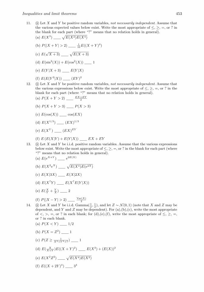
Inequalities and limit theorems 453
11. s� Let X and Y be positive random variables, not necessarily independent. Assume thatthe various expected values below exist. Write the most appropriate of , �, =, or ? inthe blank for each part (where “?” means that no relation holds in general).
(a) E(X3)p
E(X2)E(X4)
(b) P (|X + Y | > 2) 1
16
E((X + Y )4)
(c) E(pX + 3)
pE(X + 3)
(d) E(sin2(X)) + E(cos2(X)) 1
(e) E(Y |X + 3) E(Y |X)
(f) E(E(Y 2|X)) (EY )2
12. s� Let X and Y be positive random variables, not necessarily independent. Assume thatthe various expressions below exist. Write the most appropriate of , �, =, or ? in theblank for each part (where “?” means that no relation holds in general).
(a) P (X + Y > 2) EX+EY2
(b) P (X + Y > 3) P (X > 3)
(c) E(cos(X)) cos(EX)
(d) E(X1/3) (EX)1/3
(e) E(XY ) (EX)EY
(f) E (E(X|Y ) + E(Y |X)) EX + EY
13. s� Let X and Y be i.i.d. positive random variables. Assume that the various expressionsbelow exist. Write the most appropriate of , �, =, or ? in the blank for each part (where“?” means that no relation holds in general).
(a) E(eX+Y ) e2E(X)
(b) E(X2eX)p
E(X4)E(e2X)
(c) E(X|3X) E(X|2X)
(d) E(X7Y ) E(X7E(Y |X))
(e) E(XY
+ YX) 2
(f) P (|X � Y | > 2) Var(X)
2
14. s� Let X and Y be i.i.d. Gamma( 12
, 1
2
), and let Z ⇠ N (0, 1) (note that X and Z may bedependent, and Y and Z may be dependent). For (a),(b),(c), write the most appropriateof <, >, =, or ? in each blank; for (d),(e),(f), write the most appropriate of , �, =,or ? in each blank.
(a) P (X < Y ) 1/2
(b) P (X = Z2) 1
(c) P (Z � 1
X4
+Y 4
+7
) 1
(d) E( XX+Y
)E((X + Y )2) E(X2) + (E(X))2
(e) E(X2Z2)p
E(X4)E(X2)
(f) E((X + 2Y )4) 34

454 Introduction to Probability
15. Let X,Y, Z be i.i.d. N (0, 1) r.v.s. Write the most appropriate of , �, =, or ? in eachblank (where “?” means that no relation holds in general).
(a) P (X2 + Y 2 + Z2 > 6) 1/2
(b) P (X2 < 1) 2/3
(c) E⇣
X2
X2
+Y 2
+Z2
⌘1/4
(d) Var(�(X) + �(Y ) + �(Z)) 1/4
(e) E(e�X) E(eX)
(f) E(|X|eX)p
E(e2X)
16. Let X,Y, Z,W be i.i.d. positive r.v.s with CDF F and E(X) = 1. Write the mostappropriate of , �, =, or ? in each blank (where “?” means that no relation holds ingeneral).
(a) F (3) 2/3
(b) (F (3))3 P (X + Y + Z 9)
(c) E⇣
X2
X2
+Y 2
+Z2
+W2
⌘1/4
(d) E(XY ZW ) E(X4)
(e) Var(E(Y |X)) Var(Y )
(f) Cov(X + Y,X � Y ) 0
LLN and CLT
17. s� Let X1
, X2
, . . . be i.i.d. positive random variables with mean 2. Let Y1
, Y2
, . . . bei.i.d. positive random variables with mean 3. Show that
X1
+X2
+ · · ·+Xn
Y1
+ Y2
+ · · ·+ Yn! 2
3
with probability 1. Does it matter whether the Xi are independent of the Yj?
18. s� Let U1
, U2
, . . . , U60
be i.i.d. Unif(0,1) and X = U1
+ U2
+ · · ·+ U60
.
(a) Which important distribution is the distribution of X very close to? Specify whatthe parameters are, and state which theorem justifies your choice.
(b) Give a simple but accurate approximation for P (X > 17). Justify briefly.
19. s� Let Vn ⇠ �2
n and Tn ⇠ tn for all positive integers n.
(a) Find numbers an and bn such that an(Vn � bn) converges in distribution to N (0, 1).
(b) Show that T 2
n/(n+ T 2
n) has a Beta distribution (without using calculus).
20. s� Let T1
, T2
, . . . be i.i.d. Student-t r.v.s with m � 3 degrees of freedom. Find constantsan and bn (in terms of m and n) such that an(T1
+ T2
+ · · · + Tn � bn) converges toN (0, 1) in distribution as n ! 1.
21. s� (a) Let Y = eX , with X ⇠ Expo(3). Find the mean and variance of Y .
(b) For Y1
, . . . , Yn i.i.d. with the same distribution as Y from (a), what is the approxi-mate distribution of the sample mean Yn = 1
n
Pnj=1
Yj when n is large?

Inequalities and limit theorems 455
22. s� (a) Explain why the Pois(n) distribution is approximately Normal if n is a largepositive integer (specifying what the parameters of the Normal are).
(b) Stirling’s formula is an amazingly accurate approximation for factorials:
n! ⇡p2⇡n
⇣ne
⌘n
,
where in fact the ratio of the two sides goes to 1 as n ! 1. Use (a) to give aquick heuristic derivation of Stirling’s formula by using a Normal approximation tothe probability that a Pois(n) r.v. is n, with the continuity correction: first writeP (N = n) = P (n� 1
2
< N < n+ 1
2
), where N ⇠ Pois(n).
23. s� (a) Consider i.i.d. Pois(�) r.v.s X1
, X2
, . . . . The MGF of Xj is M(t) = e�(et�1). Find
the MGF Mn(t) of the sample mean Xn = 1
n
Pnj=1
Xj .
(b) Find the limit of Mn(t) as n ! 1. (You can do this with almost no calculationusing a relevant theorem; or you can use (a) and the fact that ex ⇡ 1 + x if x is verysmall.)
24. Let Xn ⇠ Pois(n) for all positive integers n. Use MGFs to show that the distribution ofthe standardized version of Xn converges to a Normal distribution as n ! 1, withoutinvoking the CLT.
25. An important concept in frequentist statistics is that of a confidence interval (CI).Suppose we observe data X from a distribution with parameter ✓. Unlike in Bayesianstatistics, ✓ is treated as a fixed but unknown constant; it is not given a prior distribution.A 95% confidence interval consists of a lower bound L(X) and upper bound U(X) suchthat
P (L(X) < ✓ < U(X)) = 0.95
for all possible values of ✓. Note that in the above statement, L(X) and U(X) arerandom variables, as they are functions of the r.v. X, whereas ✓ is a constant. Thedefinition says that the random interval (L(X), U(X)) has a 95% chance of containingthe true value of ✓.
Imagine an army of frequentists all over the world, independently generating 95% CIs.The jth frequentist observes data Xj and makes a confidence interval for the parameter✓j . Show that if there are n of these frequentists, then the fraction of their intervalswhich contain the corresponding parameter approaches 0.95 as n ! 1.
Hint: Consider the indicator r.v.s Ij = I(L(Xj) < ✓j < U(Xj)).
26. This problem extends Example 10.3.7 to a more general setting. Again, suppose a veryvolatile stock rises 70% or drops 50% in price, with equal probabilities and with di↵erentdays independent.
(a) Suppose a hedge fund manager always invests half of her current fortune into thestock each day. Let Yn be her fortune after n days, starting from an initial fortune ofY0
= 100. What happens to Yn as n ! 1?
(b) More generally, suppose the hedge fund manager always invests a fraction ↵ of hercurrent fortune into the stock each day (in Part (a), we took ↵ = 1/2). With Y
0
and Yn
defined as in Part (a), find the function g(↵) such that
log Yn
n! g(↵)
with probability 1 as n ! 1, and prove that g(↵) is maximized when ↵ = 3/8.
Mixed practice
27. As in Exercise 36 from Chapter 3, there are n voters in an upcoming election in a certaincountry, where n is a large, even number. There are two candidates, A and B. Each voterchooses randomly whom to vote for, independently and with equal probabilities.

456 Introduction to Probability
(a) Use a Normal approximation (with continuity correction) to get an approximationfor the probability of a tie, in terms of �.
(b) Use a first-order Taylor expansion (linear approximation) to the approximationfrom Part (a) to show that the probability of a tie is approximately 1/
pcn, where c is
a constant (which you should specify).
28. A handy rule of thumb in statistics and life is as follows:
Conditioning often makes things better.
This problem explores how the above rule of thumb applies to estimating unknownparameters. Let ✓ be an unknown parameter that we wish to estimate based on dataX
1
, X2
, . . . , Xn (these are r.v.s before being observed, and then after the experimentthey “crystallize” into data). In this problem, ✓ is viewed as an unknown constant, andis not treated as an r.v. as in the Bayesian approach. Let T
1
be an estimator for ✓ (thismeans that T
1
is a function of X1
, . . . , Xn which is being used to estimate ✓).
A strategy for improving T1
(in some problems) is as follows. Suppose that we have anr.v. R such that T
2
= E(T1
|R) is a function of X1
, . . . , Xn (in general, E(T1
|R) mightinvolve unknowns such as ✓ but then it couldn’t be used as an estimator). Also supposethat P (T
1
= T2
) < 1, and that E(T 2
1
) is finite.
(a) Use Jensen’s inequality to show that T2
is better than T1
in the sense that the meansquared error is less, i.e.,
E(T2
� ✓)2 < E(T1
� ✓)2.
Hint: Use Adam’s law on the right-hand side.
(b) The bias of an estimator T for ✓ is defined to be b(T ) = E(T ) � ✓. An importantidentity in statistics, a form of the bias-variance tradeo↵, is that mean squared error isvariance plus squared bias:
E(T � ✓)2 = Var(T ) + (b(T ))2.
Use this identity and Eve’s law to give an alternative proof of the result from (a).
(c) Now suppose that X1
, X2
, . . . are i.i.d. with mean ✓, and consider the special caseT1
= X1
, R =Pn
j=1
Xj . Find T2
in simplified form, and check that it has lower meansquared error than T
1
for n � 2. Also, say what happens to T1
and T2
as n ! 1.
29. Each page of an n-page book has a Pois(�) number of typos, where � is unknown (butis not treated as an r.v.). Typos on di↵erent pages are independent. Thus we havei.i.d. X
1
, . . . , Xn ⇠ Pois(�), where Xj is the number of typos on page j. Suppose we areinterested in estimating the probability ✓ that a page has no typos:
✓ = P (Xj = 0) = e��.
(a) Let Xn = 1
n(X
1
+ · · ·+Xn). Show that Tn = e�¯Xn is biased for ✓. (In other words,
E(T )� ✓ 6= 0.)
(b) Show that as n ! 1, Tn ! ✓ with probability 1.
(c) Show that W = 1
n(I(X
1
= 0) + · · · + I(Xn = 0)) is unbiased for ✓. Using the
fact that X1
|(X1
+ · · · + Xn = s) ⇠ Bin(s, 1/n), find E(W |X1
+ · · · + Xn). Is W =E(W |X
1
+ · · ·+Xn) also unbiased for ✓?
(d) Using Eve’s law or otherwise, show that W has lower variance than W , and relatethis to the previous question.

Inequalities and limit theorems 457
30. A binary sequence is being generated through some process (random or deterministic).You need to sequentially predict each new number, i.e, you predict whether the nextnumber will be 0 or 1, then observe it, then predict the next number, etc. Each of yourpredictions can be based on the entire past history of the sequence.
(a) Suppose for this part that the binary sequence consists of i.i.d. Bern(p) r.v.s, withp known. What is your optimal strategy (for each prediction, your goal is to maximizethe probability of being correct)? What is the probability that you will guess the nthvalue correctly with this strategy?
(b) Now suppose that the binary sequence consists of i.i.d. Bern(p) r.v.s, with p unknown.Consider the following strategy: say 1 as your first prediction; after that, say “1” if theproportion of 1’s so far is at least 1/2, and say “0” otherwise. Find the limit as n ! 1of the probability of guessing the nth value correctly (in terms of p).
(c) Now suppose that you follow the strategy from (b), but that the binary sequenceis generated by a nefarious entity who knows your strategy. What can the entity do tomake your guesses be wrong as often as possible?
31. s� Let X and Y be independent standard Normal r.v.s and let R2 = X2 + Y 2 (whereR > 0 is the distance from (X,Y ) to the origin).
(a) The distribution of R2 is an example of three of the important distributions wehave seen. State which three of these distributions R2 is an instance of, specifying theparameter values.
(b) Find the PDF of R.
Hint: Start with the PDF fW (w) of W = R2.
(c) Find P (X > 2Y + 3) in terms of the standard Normal CDF �.
(d) Compute Cov(R2, X). Are R2 and X independent?
32. s� Let Z1
, . . . , Zn ⇠ N (0, 1) be i.i.d.
(a) As a function of Z1
, create an Expo(1) r.v. X (your answer can also involve thestandard Normal CDF �).
(b) Let Y = e�R, where R =p
Z2
1
+ · · ·+ Z2
n. Write down (but do not evaluate) anintegral for E(Y ).
(c) Let X1
= 3Z1
� 2Z2
and X2
= 4Z1
+ 6Z2
. Determine whether X1
and X2
areindependent (be sure to mention which results you’re using).
33. s� Let X1
, X2
, . . . be i.i.d. positive r.v.s. with mean µ, and let Wn = X1
X1
+···+Xn
.
(a) Find E(Wn).
Hint: Consider X1
X1
+···+Xn
+ X2
X1
+···+Xn
+ · · ·+ Xn
X1
+···+Xn
.
(b) What random variable does nWn converge to (with probability 1) as n ! 1?
(c) For the case that Xj ⇠ Expo(�), find the distribution of Wn, preferably withoutusing calculus. (If it is one of the named distributions, state its name and specify theparameters; otherwise, give the PDF.)
34. Let X1
, X2
, . . . be i.i.d. Expo(1).
(a) Let N = min{n : Xn � 1} be the index of the first Xj to exceed 1. Find thedistribution of N � 1 (give the name and parameters), and hence find E(N).
(b) Let M = min{n : X1
+X2
+ · · ·+Xn � 10} be the number of Xj ’s we observe untiltheir sum exceeds 10 for the first time. Find the distribution of M � 1 (give the nameand parameters), and hence find E(M).
Hint: Consider a Poisson process.
(c) Let Xn = (X1
+ · · ·+Xn)/n. Find the exact distribution of Xn (give the name andparameters), as well as the approximate distribution of Xn for n large (give the nameand parameters).


11
Markov chains
Markov chains were first introduced in 1906 by Andrey Markov (of Markov’s in-equality), with the goal of showing that the law of large numbers can apply torandom variables that are not independent. To see where the Markov model comesfrom, start by considering an i.i.d. sequence of random variables X
0
, X1
, . . . , Xn, . . .where we think of n as time. This is the setting we worked in throughout Chapter10, but for modeling real-world phenomena, independence can be an excessively re-strictive assumption; it means that the Xn provide absolutely no information abouteach other. At the other extreme, allowing arbitrary interactions between the Xn
makes it very di�cult to compute even basic things. A Markov chain is a sequenceof r.v.s that exhibits one-step dependence, in a precise sense that we shall soondefine. Thus Markov chains are a happy medium between complete independenceand complete dependence.
Since their invention, Markov chains have become extremely important in a hugenumber of fields such as biology, game theory, finance, machine learning, and statisti-cal physics. They are also very widely used for simulations of complex distributions,via algorithms known as Markov chain Monte Carlo (MCMC). In this chapter wewill introduce Markov chains and their properties, and in the next chapter we’lllook at some examples of MCMC techniques.
11.1 Markov property and transition matrix
Markov chains “live” in both space and time: the set of possible values of the Xn iscalled the state space, and the index n represents the evolution of the process overtime. The state space of a Markov chain can be either discrete or continuous, andtime can also be either discrete or continuous (in the continuous-time setting, wewould imagine a process Xt defined for all real t � 0). In this chapter we will focusexclusively on discrete-state, discrete-time Markov chains, with a finite state space.Specifically, we will assume that the Xn take values in a finite set, which we usuallytake to be {1, 2, . . . ,M} or {0, 1, . . . ,M}.
Definition 11.1.1 (Markov chain). A sequence of random variables X0
, X1
, X2
, . . .taking values in the state space {1, 2, . . . ,M} is called aMarkov chain if for all n � 0,
P (Xn+1
= j|Xn = i,Xn�1
= in�1
, . . . , X0
= i0
) = P (Xn+1
= j|Xn = i).
459

460 Introduction to Probability
The quantity P (Xn+1
= j|Xn = i) is called the transition probability from statei to state j. In this book, when referring to a Markov chain we will implicitlyassume that it is time-homogeneous, which means that the transition probabilityP (Xn+1
= j|Xn = i) is the same for all times n. But care is needed, since theliterature is not consistent about whether to say “time-homogeneous Markov chain”or just “Markov chain”.
The above condition is called the Markov property , and it says that given the en-tire past history X
0
, X1
, X2
, . . . , Xn, only the most recent term, Xn, matters forpredicting Xn+1
. If we think of time n as the present, times before n as the past,and times after n as the future, the Markov property says that given the present,the past and future are conditionally independent. The Markov property greatlysimplifies computations of conditional probability: instead of having to conditionon the entire past, we only need to condition on the most recent value.
To describe the dynamics of a Markov chain, we need to know the probabilitiesof moving from any state to any other state, that is, the probabilities P (Xn+1
=j|Xn = i) on the right-hand side of the Markov property. This information can beencoded in a matrix, called the transition matrix, whose (i, j) entry is the probabilityof going from state i to state j in one step of the chain.
Definition 11.1.2 (Transition matrix). Let X0
, X1
, X2
, . . . be a Markov chainwith state space {1, 2, . . . ,M}, and let qij = P (Xn+1
= j|Xn = i) be the transitionprobability from state i to state j. The M ⇥ M matrix Q = (qij) is called thetransition matrix of the chain.
Note that Q is a nonnegative matrix in which each row sums to 1. This is because,starting from any state i, the events “move to 1”, “move to 2”, . . . , “move toM” are disjoint, and their union has probability 1 because the chain has to gosomewhere.
Example 11.1.3 (Rainy-sunny Markov chain). Suppose that on any given day,the weather can either be rainy or sunny. If today is rainy, then tomorrow will berainy with probability 1/3 and sunny with probability 2/3. If today is sunny, thentomorrow will be rainy with probability 1/2 and sunny with probability 1/2. LettingXn be the weather on day n, X
0
, X1
, X2
, . . . is a Markov chain on the state space{R,S}, where R stands for rainy and S for sunny. We know that the Markov prop-erty is satisfied because, from the description of the process, only today’s weathermatters for predicting tomorrow’s.
The transition matrix of the chain is
✓ R S
R 1/3 2/3S 1/2 1/2
◆.
The first row says that starting from state R, we transition back to state R withprobability 1/3 and transition to state S with probability 2/3. The second row says

Markov chains 461
that starting from state S, we have a 1/2 chance of moving to state R and a 1/2chance of staying in state S. We could just as well have used
✓ S R
S 1/2 1/2R 2/3 1/3
◆
as our transition matrix instead. In general, if there isn’t an obvious ordering ofthe states of a Markov chain (as with the states R and S), we just need to fix anordering of the states and use it consistently.
The transition probabilities of a Markov chain can also be represented with a di-agram. Each state is represented by a circle, and the arrows indicate the possibleone-step transitions; we can imagine a particle wandering around from state tostate, randomly choosing which arrow to follow. Next to the arrows we write thecorresponding transition probabilities.
SR1/31/2
2/3
1/2
What if the weather tomorrow depended on the weather today and the weatheryesterday? For example, suppose that the weather behaves as above, except thatif there have been two consecutive days of rain, then tomorrow will definitely besunny, and if there have been two consecutive days of sun, then tomorrow willdefinitely be rainy. Under these new weather dynamics, the Xn no longer form aMarkov chain, as the Markov property is violated: conditional on today’s weather,yesterday’s weather can still provide useful information for predicting tomorrow’sweather.
However, by enlarging the state space, we can create a new Markov chain: letYn = (Xn�1
, Xn) for n � 1. Then Y1
, Y2
, . . . is a Markov chain on the state space{(R,R), (R,S), (S,R), (S, S)}. You can verify that the transition matrix of this chainis
0
BB@
(R,R) (R,S) (S,R) (S, S)
(R,R) 0 1 0 0(R,S) 0 0 1/2 1/2(S,R) 1/3 2/3 0 0(S, S) 0 0 1 0
1
CCA
and that its corresponding graphical representation is given in the following figure.

462 Introduction to Probability
RSRR
1
SSSR1
1/3 2/3
1/2 1/2
Similarly, we could handle third-order or fourth-order dependencies in the weatherby further enlarging the state space to make the Markov property hold. ⇤
Once we have the transition matrix Q of a Markov chain, we can work out thetransition probabilities for longer timescales.
Definition 11.1.4 (n-step transition probability). The n-step transition probabil-ity from i to j is the probability of being at j exactly n steps after being at i. We
denote this by q(n)ij :
q(n)ij = P (Xn = j|X
0
= i).
Note that
q(2)
ij =X
k
qikqkj
since to get from i to j in two steps, the chain must go from i to some intermediarystate k, and then from k to j; these transitions are independent because of theMarkov property. Since the right-hand side is the (i, j) entry of Q2 by the definitionof matrix multiplication, we conclude that the matrix Q2 gives the two-step tran-sition probabilities. By induction, the nth power of the transition matrix gives then-step transition probabilities:
q(n)ij is the (i, j) entry of Qn.
Example 11.1.5 (Transition matrix of 4-state Markov chain). Consider the 4-stateMarkov chain depicted in Figure 11.1. When no probabilities are written over thearrows, as in this case, it means all arrows originating from a given state are equallylikely. For example, there are 3 arrows originating from state 1, so the transitions1 ! 3, 1 ! 2, and 1 ! 1 all have probability 1/3. Therefore the transition matrix

Markov chains 463
1
2
3 4
FIGURE 11.1
A 4-state Markov chain.
of the chain is
Q =
0
BBBBBBBBB@
1/3 1/3 1/3 0
0 0 1/2 1/2
0 1 0 0
1/2 0 0 1/2
1
CCCCCCCCCA
.
To compute the probability that the chain is in state 3 after 5 steps, starting atstate 1, we would look at the (1,3) entry of Q5. Here (using a computer to find Q5),
Q5 =
0
BBBBBBBBB@
853/3888 509/1944 52/243 395/1296
173/864 85/432 31/108 91/288
37/144 29/72 1/9 11/48
499/2592 395/1296 71/324 245/864
1
CCCCCCCCCA
,
so q(5)
13
= 52/243. ⇤
Using the language of Chapter 7, the transition matrix Q encodes the conditionaldistributions of X
1
given the initial state of the chain. Specifically, the ith row ofQ is the conditional PMF of X
1
given X0
= i, displayed as a row vector. Similarly,the ith row of Qn is the conditional PMF of Xn given X
0
= i.
To get the marginal distributions of X0
, X1
, . . . , we need to specify not just thetransition matrix, but also the initial conditions of the chain. This can be done bysetting the initial state X
0
to be a particular state, or by randomly choosing X0
according to some distribution. Let (t1
, t2
, . . . , tM ) be the PMF of X0
displayed asa vector, that is, ti = P (X
0
= i). Then the marginal distribution of the chain at
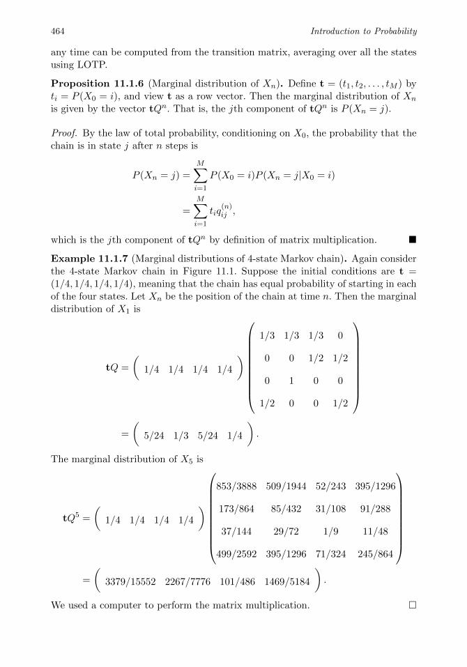
464 Introduction to Probability
any time can be computed from the transition matrix, averaging over all the statesusing LOTP.
Proposition 11.1.6 (Marginal distribution of Xn). Define t = (t1
, t2
, . . . , tM ) byti = P (X
0
= i), and view t as a row vector. Then the marginal distribution of Xn
is given by the vector tQn. That is, the jth component of tQn is P (Xn = j).
Proof. By the law of total probability, conditioning on X0
, the probability that thechain is in state j after n steps is
P (Xn = j) =MX
i=1
P (X0
= i)P (Xn = j|X0
= i)
=MX
i=1
tiq(n)ij ,
which is the jth component of tQn by definition of matrix multiplication. ⌅Example 11.1.7 (Marginal distributions of 4-state Markov chain). Again considerthe 4-state Markov chain in Figure 11.1. Suppose the initial conditions are t =(1/4, 1/4, 1/4, 1/4), meaning that the chain has equal probability of starting in eachof the four states. Let Xn be the position of the chain at time n. Then the marginaldistribution of X
1
is
tQ =
✓1/4 1/4 1/4 1/4
◆
0
BBBBBBBBB@
1/3 1/3 1/3 0
0 0 1/2 1/2
0 1 0 0
1/2 0 0 1/2
1
CCCCCCCCCA
=
✓5/24 1/3 5/24 1/4
◆.
The marginal distribution of X5
is
tQ5 =
✓1/4 1/4 1/4 1/4
◆
0
BBBBBBBBB@
853/3888 509/1944 52/243 395/1296
173/864 85/432 31/108 91/288
37/144 29/72 1/9 11/48
499/2592 395/1296 71/324 245/864
1
CCCCCCCCCA
=
✓3379/15552 2267/7776 101/486 1469/5184
◆.
We used a computer to perform the matrix multiplication. ⇤

Markov chains 465
11.2 Classification of states
In this section we introduce terminology for describing the various characteristicsof a Markov chain. The states of a Markov chain can be classified as recurrent ortransient, depending on whether they are visited over and over again in the longrun or are eventually abandoned. States can also be classified according to theirperiod, which is a positive integer summarizing the amount of time that can elapsebetween successive visits to a state. These characteristics are important becausethey determine the long-run behavior of the Markov chain, which we will study inSection 11.3.
The concepts of recurrence and transience are best illustrated with a concrete ex-ample. In the Markov chain shown on the left of Figure 11.2 (previously featuredin Example 11.1.5), a particle moving around between states will continue to spendtime in all 4 states in the long run, since it is possible to get from any state to anyother state. In contrast, consider the chain on the right of Figure 11.2, and let theparticle start at state 1. For a while, the chain may linger in the triangle formed bystates 1, 2, and 3, but eventually it will reach state 4, and from there it can neverreturn to states 1, 2, or 3. It will then wander around between states 4, 5, and 6forever. States 1, 2, and 3 are transient and states 4, 5, and 6 are recurrent.
1
2
3 4 1
2
3
4
5
6
FIGURE 11.2
Left: 4-state Markov chain with all states recurrent. Right: 6-state Markov chainwith states 1, 2, and 3 transient.
In general, these concepts are defined as follows.
Definition 11.2.1 (Recurrent and transient states). State i of a Markov chain isrecurrent if starting from i, the probability is 1 that the chain will eventually returnto i. Otherwise, the state is transient, which means that if the chain starts from i,there is a positive probability of never returning to i.

466 Introduction to Probability
In fact, although the definition of a transient state only requires that there be apositive probability of never returning to the state, we can say something stronger:as long as there is a positive probability of leaving i forever, the chain eventuallywill leave i forever. In the long run, anything that can happen, will happen (with afinite state space). We can make this statement precise with the following proposi-tion.
Proposition 11.2.2 (Number of returns to transient state is Geometric). Let i bea transient state of a Markov chain. Suppose the probability of never returning toi, starting from i, is a positive number p > 0. Then, starting from i, the number oftimes that the chain returns to i before leaving forever is distributed Geom(p).
The proof is by the story of the Geometric distribution: each time that the chainis at i, we have a Bernoulli trial which results in “failure” if the chain eventuallyreturns to i and “success” if the chain leaves i forever; these trials are independentby the Markov property. The number of returns to state i is simply the number offailures before the first success, which is the story of the Geometric distribution.In particular, since a Geometric random variable always takes finite values, thisproposition tells us that after a finite number of visits, the chain will leave state iforever.
If the number of states is not too large, one way to classify states as recurrentor transient is to draw a diagram of the Markov chain and use the same kind ofreasoning that we used when analyzing the chains in Figure 11.2. A special casewhere we can immediately conclude all states are recurrent is when the chain isirreducible, meaning that it is possible to get from any state to any other state.
Definition 11.2.3 (Irreducible and reducible chain). A Markov chain with transi-tion matrix Q is irreducible if for any two states i and j, it is possible to go from ito j in a finite number of steps (with positive probability). That is, for any statesi, j there is some positive integer n such that the (i, j) entry of Qn is positive. AMarkov chain that is not irreducible is called reducible.
Proposition 11.2.4 (Irreducible implies all states recurrent). In an irreducibleMarkov chain with a finite state space, all states are recurrent.
Proof. It is clear that at least one state must be recurrent; if all states were transient,the chain would eventually leave all states forever and have nowhere to go! So assumewithout loss of generality that state 1 is recurrent, and consider any other state i.
We know that q(n)1i is positive for some n, by the definition of irreducibility. Thus,
every time the chain is at state 1, it has a positive probability of going to statei in n steps. Since the chain visits state 1 infinitely often, we know the chain willeventually reach state i from state 1; think of each visit to state 1 as starting a trial,where “success” is defined as reaching state i in at most n steps. From state i, thechain will return to state 1 because state 1 is recurrent, and by the same logic, itwill eventually reach state i again. By induction, the chain will visit state i infinitelyoften. Since i was arbitrary, we conclude that all states are recurrent. ⌅

Markov chains 467
The converse of the proposition is false; it is possible to have a reducible Markovchain whose states are all recurrent. An example is given by the Markov chain below,which consists of two “islands” of states.
21
3
54
6
h 11.2.5. Note that recurrence or transience is a property of the states in a Markovchain, while irreducibility or reducibility is a property of the chain as a whole.
Here are two familiar problems from earlier chapters, viewed through the lens ofMarkov chains. For each, we’ll identify the recurrent and transient states.
Example 11.2.6 (Gambler’s ruin as a Markov chain). In the gambler’s ruin prob-lem, two gamblers, A and B, start with i and N � i dollars respectively, making asequence of bets for $1. In each round, player A has probability p of winning andprobability q = 1� p of losing. Let Xn be the wealth of gambler A at time n. ThenX
0
, X1
, . . . is a Markov chain on the state space {0, 1, . . . , N}. By design, X0
= i.
0 21 NN – 1...p
q
p p p
qqq1
1
Once the Markov chain reaches 0 or N , signifying bankruptcy for player A or playerB, the Markov chain stays in that state forever. We proved in Chapter 2 that theprobability that either A or B goes bankrupt is 1, so for any starting state i otherthan 0 or N , the Markov chain will eventually be absorbed into state 0 or N , neverreturning to i. Therefore, for this Markov chain, states 0 and N are recurrent, andall other states are transient. The chain is reducible because from state 0 it is onlypossible to go to state 0, and from state N it is only possible to go to state N . ⇤Example 11.2.7 (Coupon collector as a Markov chain). In the coupon collectorproblem, there are C types of coupons, which we collect one by one, sampling withreplacement from the C coupon types each time. Let Xn be the number of distinctcoupon types in our collection after n attempts. Then X
0
, X1
, . . . is a Markov chainon the state space {0, 1, . . . , C}. By design, X
0
= 0.
0 21 CC – 1...1 1/C(C – 1)/C
(C – 1)/C 11/C 2/C
(C – 2)/C 2/C

468 Introduction to Probability
In this Markov chain, with the exception of state C, we can never return to a stateafter leaving it; the number of coupon types in the collection can only increase withtime, never decrease. Thus all states are transient except for C, which is recurrent.The chain is reducible because it is not possible to go from state 2 back to state 1,for example. ⇤
Another way to classify states is according to their periods. The period of a statesummarizes how much time can elapse between successive visits to the state.
Definition 11.2.8 (Period of a state, periodic and aperiodic chain). The period ofa state i in a Markov chain is the greatest common divisor (gcd) of the possiblenumbers of steps it can take to return to i when starting at i. That is, the periodof i is the greatest common divisor of numbers n such that the (i, i) entry of Qn
is positive. (The period of i is undefined if it’s impossible ever to return to i afterstarting at i.) A state is called aperiodic if its period equals 1, and periodic other-wise. The chain itself is called aperiodic if all its states are aperiodic, and periodicotherwise.
1
2
3 4 1
2
3
4
5
6
FIGURE 11.3
Left: an aperiodic Markov chain. Right: a periodic Markov chain in which states 1,2, and 3 have period 3.
For example, let’s consider again the two Markov chains from Figure 11.2, shownagain in Figure 11.3. We first consider the 6-state chain on the right. Starting fromstate 1, it is possible to be back at state 1 after 3 steps, 6 steps, 9 steps, etc., but itis not possible to be back at state 1 after any number of steps that is not a multipleof 3. Therefore, state 1 has period 3. Similarly, states 2 and 3 also have period 3.On the other hand, states 4, 5, and 6 have period 1, but the chain is periodic sinceat least one state does not have period 1. By contrast, in the chain on the left allstates are aperiodic, so that chain is aperiodic.
In the gambler’s ruin chain, each state has period 2 except for 0 and N , which haveperiod 1. In the coupon collector chain, each state has period 1 except for state 0,

Markov chains 469
which has period 1 because it’s impossible to return to state 0. So neither of thesechains is aperiodic.
11.3 Stationary distribution
The concepts of recurrence and transience are important for understanding the long-run behavior of a Markov chain. At first, the chain may spend time in transientstates. Eventually though, the chain will spend all its time in recurrent states. Butwhat fraction of the time will it spend in each of the recurrent states? This questionis answered by the stationary distribution of the chain, also known as the steady-state distribution. We will learn in this section that for irreducible and aperiodicMarkov chains, the stationary distribution describes the long-run behavior of thechain, regardless of its initial conditions.
Definition 11.3.1 (Stationary distribution). A row vector s = (s1
, . . . , sM ) suchthat si � 0 and
Pi si = 1 is a stationary distribution for a Markov chain with
transition matrix Q if X
i
siqij = sj
for all j, or equivalently,sQ = s.
Recall that if s is the distribution of X0
, then sQ is the marginal distribution ofX
1
. Thus the equation sQ = s means that if X0
has distribution s, then X1
alsohas distribution s. But then X
2
also has distribution s, as does X3
, etc. That is, aMarkov chain whose initial distribution is the stationary distribution s will stay inthe stationary distribution forever.
One way to visualize the stationary distribution of a Markov chain is to imaginea large number of particles, each independently bouncing from state to state ac-cording to the transition probabilities. After a while, the system of particles willapproach an equilibrium where, at each time period, the number of particles leav-ing a state will be counterbalanced by the number of particles entering that state,and this will be true for all states. As a result, the system as a whole will appearto be stationary, and the proportion of particles in each state will be given by thestationary distribution.
h 11.3.2 (Stationary distribution is marginal, not conditional). When a Markovchain is at the stationary distribution, the unconditional PMF of Xn equals s forall n, but the conditional PMF of Xn given Xn�1
= i is still encoded by the ith rowof the transition matrix Q.
If a Markov chain starts at the stationary distribution, then all of the Xn are iden-tically distributed (since they have the same marginal distribution s), but they are

470 Introduction to Probability
not necessarily independent, since the conditional distribution of Xn given Xn�1
= iis, in general, di↵erent from the marginal distribution of Xn.
h 11.3.3 (Sympathetic magic). If a Markov chain starts at the stationary distri-bution, then the marginal distributions of the Xn are all equal. This is not the sameas saying that the Xn themselves are all equal; confusing the random variables Xn
with their distributions is an example of sympathetic magic.
For very small Markov chains, we may solve for the stationary distribution by hand,using the definition. The next example illustrates this for a two-state chain.
Example 11.3.4 (Stationary distribution for a two-state chain). Let
Q =
0
B@1/3 2/3
1/2 1/2
1
CA .
The stationary distribution is of the form s = (s, 1� s), and we must solve for s inthe system
✓s 1� s
◆0
B@1/3 2/3
1/2 1/2
1
CA =
✓s 1� s
◆,
which is equivalent to
1
3s+
1
2(1� s) = s,
2
3s+
1
2(1� s) = 1� s.
The only solution is s = 3/7, so (3/7, 4/7) is the unique stationary distribution ofthe Markov chain. ⇤In terms of linear algebra, the equation sQ = s says that s is a left eigenvector ofQ with eigenvalue 1 (see Section A.3 of the math appendix for more details). Toget the usual kind of eigenvector (a right eigenvector), take transposes: Q0s0 = s0,where the 0 symbol denotes taking the transpose.
11.3.1 Existence and uniqueness
Does a stationary distribution always exist, and is it unique? It turns out that for afinite state space, a stationary distribution always exists. Furthermore, in irreducibleMarkov chains, the stationary distribution is unique.
Theorem 11.3.5 (Existence and uniqueness of stationary distribution). Any ir-reducible Markov chain has a unique stationary distribution. In this distribution,every state has positive probability.

Markov chains 471
The theorem is a consequence of a result from linear algebra called the Perron-Frobenius theorem, which is stated in Section A.3 of the math appendix.
The 4-state chain on the left of Figure 11.3 is irreducible: in terms of the picture, itis possible to go from anywhere to anywhere following the arrows; in terms of thetransition matrix, all the entries of Q5 are positive. Therefore, by Theorem 11.3.5,the chain has a unique stationary distribution. On the other hand, the gambler’s ruinchain is reducible, so the theorem does not apply. It turns out that the gambler’s ruinchain does not have a unique stationary distribution: in the long run, the chain caneither converge to a degenerate distribution at state 0, or a degenerate distributionat state N .
11.3.2 Convergence
We have already informally stated that the stationary distribution describes thelong-run behavior of the chain, in the sense that if we run the chain for a long time,the marginal distribution of Xn converges to the stationary distribution s. The nexttheorem states that this is true as long as the chain is both irreducible and aperiodic.Then, regardless of the chain’s initial conditions, the PMF of Xn will converge tothe stationary distribution as n ! 1. This relates the concept of stationarity tothe long-run behavior of a Markov chain. The proof is omitted.
Theorem 11.3.6 (Convergence to stationary distribution). Let X0
, X1
, . . . be aMarkov chain with stationary distribution s and transition matrix Q, such thatsome power Qm is positive in all entries. (These assumptions are equivalent toassuming that the chain is irreducible and aperiodic.) Then P (Xn = i) converges tosi as n ! 1. In terms of the transition matrix, Qn converges to a matrix in whicheach row is s.
Therefore, after a large number of steps, the probability that the chain is in state iis close to the stationary probability si, regardless of the chain’s initial conditions.Intuitively, the extra condition of aperiodicity is needed in order to rule out chainsthat just go around in circles, such as the chain in the following example.
Example 11.3.7 (Periodic chain). Figure 11.4 shows a periodic Markov chainwhere each state has period 5.
5
4 3
2
1
FIGURE 11.4
A periodic chain.

472 Introduction to Probability
The transition matrix of the chain is
Q =
0
BBBBBBBBBBBB@
0 1 0 0 0
0 0 1 0 0
0 0 0 1 0
0 0 0 0 1
1 0 0 0 0
1
CCCCCCCCCCCCA
.
It can be verified without much di�culty that s = (1/5, 1/5, 1/5, 1/5, 1/5) is astationary distribution of this chain, and by Theorem 11.3.5, s is unique. However,suppose the chain starts at X
0
= 1. Then the PMF of Xn assigns probability 1to the state (n mod 5) + 1 and 0 to all other states, so it does not converge to sas n ! 1. Nor does Qn converge to a matrix in which each row is s: the chain’stransitions are deterministic, so Qn always consists of 0’s and 1’s. ⇤Lastly, the stationary distribution tells us the average time between visits to astate.
Theorem 11.3.8 (Expected time to return). Let X0
, X1
, . . . be an irreducibleMarkov chain with stationary distribution s. Let ri be the expected time it takesthe chain to return to i, given that it starts at i. Then si = 1/ri.
Here is how the theorems apply to the two-state chain from Example 11.3.4.
Example 11.3.9 (Long-run behavior of a two-state chain). In the long run, thechain in Example 11.3.4 will spend 3/7 of its time in state 1 and 4/7 of its time instate 2. Starting at state 1, it will take an average of 7/3 steps to return to state1. The powers of the transition matrix converge to a matrix where each row is thestationary distribution:
0
B@1/3 2/3
1/2 1/2
1
CA
n
!
0
B@3/7 4/7
3/7 4/7
1
CA as n ! 1.
⇤
11.3.3 Google PageRank
We next consider a vastly larger example of a stationary distribution, for a Markovchain on a state space with billions of interconnected nodes: the World Wide Web.The next example explains how the founders of Google modeled web-surfing as aMarkov chain, and then used its stationary distribution to rank the relevance ofwebpages. For years Google described the resulting method, known as PageRank ,as “the heart of our software”.

Markov chains 473
Suppose you are interested in a certain topic, say chess, so you use a search engineto look for useful webpages with information about chess. There are millions ofwebpages that mention the word “chess”, so a key issue a search engine needs todeal with is what order to show the search results in. It would be a disaster to haveto wade through thousands of garbage pages that mention “chess” before findinginformative content.
In the early days of the web, various approaches to this ranking problem wereused. For example, some search engines employed people to manually decide whichpages were most useful, like a museum curator. But aside from being subjectiveand expensive, this quickly became infeasible as the web grew. Others focused onthe number of times the search term was mentioned on the site. But a page thatmentions “chess” over and over again could easily be less useful than a concisereference page or a page about chess that doesn’t repeatedly mention the word.Furthermore, this method is very open to abuse: a spam page could boost its rankingjust by including a long list of words repeated over and over again.
Both of the above methods ignore the structure of the web: which pages link to whichother pages? Taking the link structure into account led to dramatic improvementsin search engines. As a first attempt, one could rank a page based on how manyother pages link to it. That is, if Page A links to Page B, we consider it a “vote”for B, and we rank pages based on how many votes they have.
But this is again very open to abuse: a spam page could boost its ranking by creatingthousands of other spam pages linking to it. And though it may seem democraticfor each page to have equal voting power, an incoming link from a reliable page ismore meaningful than a link from an uninformative page. Google PageRank, whichwas introduced in 1998 by Sergey Brin and the aptly named Larry Page, ranksthe importance of a page not only by how many pages link to it, but also by theimportance of those pages.
Consider the web as a directed network—which is what it is. Each page on theweb is a node, and links between nodes represent links between pages. For exam-ple, suppose for simplicity that the web only has 4 pages, connected as shown inFigure 11.5.
1 2
3 4
FIGURE 11.5
It’s a small web after all.
Imagine someone randomly surfing the web, starting at some page and then ran-

474 Introduction to Probability
domly clicking links to go from one page to the next (with equal probabilities forall links on the current page). The idea of PageRank is to measure the importanceof a page by the long-run fraction of time spent at that page.
Of course, some pages may have no outgoing links at all, such as page 4 above. Whenthe web surfer encounters such a page, rather than despairing he or she opens up anew browser window and visits a uniformly random page. Thus a page with no linksis converted to a page that links to every page, including itself. For the exampleabove, the resulting transition matrix is
Q =
0
BBBBBBBBB@
0 1/2 0 1/2
1/2 0 1/2 0
0 0 0 1
1/4 1/4 1/4 1/4
1
CCCCCCCCCA
.
In general, let M be the number of pages on the web, let Q be the M by M tran-sition matrix of the chain described above, and let s be the stationary distribution(assuming it exists and is unique). Think of sj as a measure of how important Pagej is. Intuitively, the equation
sj =X
i
siqij
says that the score of Page j should be based not only on how many other pages linkto it, but on their scores. Furthermore, the “voting power” of a page gets diluted ifit has a lot of outgoing links: it counts for more if page i’s only link is to page j (sothat qij = 1) than if page i has thousands of links, one of which happens to be topage j.
It is not clear that a unique stationary distribution exists for this chain, since it maynot be irreducible and aperiodic. Even if it is irreducible and aperiodic, convergenceto the stationary distribution could be very slow since the web is so immense. Toaddress these issues, suppose that before each move, the web surfer flips a coinwith probability ↵ of Heads. If Heads, the web surfer clicks a random link from thecurrent page; if Tails, the web surfer teleports to a uniformly random page. Theresulting chain has the Google transition matrix
G = ↵Q+ (1� ↵)J
M,
where J is the M by M matrix of all 1’s. Note that the row sums of G are 1 andthat all entries are positive, so G is a valid transition matrix for an irreducible,aperiodic Markov chain. This means there is a unique stationary distribution s,called PageRank, and the chain will converge to it! The choice of ↵ is an importantconsideration; choosing ↵ close to 1 makes sense to respect the structure of theweb as much as possible, but there is a tradeo↵ since it turns out that smaller

Markov chains 475
values of ↵ make the chain converge much faster. As a compromise, the originalrecommendation of Brin and Page was ↵ = 0.85.
PageRank is conceptually nice, but computing it sounds extremely di�cult, consid-ering that sG = s could be a system of 100 billion equations in 100 billion unknowns.Instead of thinking of this as a massive algebra problem, we can use the Markovchain interpretation: for any starting distribution t, tGn ! s as n ! 1. And tG iseasier to compute than it might seem at first:
tG = ↵(tQ) +1� ↵
M(tJ),
where computing the first term isn’t too hard since Q is very sparse (mostly 0’s) andcomputing the second term is easy since tJ is a vector of all 1’s. Then tG becomesthe new t, and we can compute tG2 = (tG)G, etc., until the sequence appears tohave converged (though it is hard to know that it has converged). This gives anapproximation to PageRank, and has an intuitive interpretation as the distributionof where the web surfer is after a large number of steps.
11.4 Reversibility
We have seen that the stationary distribution of a Markov chain is extremely usefulfor understanding its long-run behavior. Unfortunately, in general it may be compu-tationally di�cult to find the stationary distribution when the state space is large.This section addresses an important special case where working with eigenvalueequations for large matrices can be avoided.
Definition 11.4.1 (Reversibility). Let Q = (qij) be the transition matrix of aMarkov chain. Suppose there is s = (s
1
, . . . , sM ) with si � 0,P
i si = 1, such that
siqij = sjqji
for all states i and j. This equation is called the reversibility or detailed balancecondition, and we say that the chain is reversible with respect to s if it holds.
Given a transition matrix, if we can find a nonnegative vector s whose componentssum to 1 and which satisfies the reversibility condition, then s is automatically astationary distribution.
Proposition 11.4.2 (Reversible implies stationary). Suppose that Q = (qij) isa transition matrix of a Markov chain that is reversible with respect to a nonneg-ative vector s = (s
1
, . . . , sM ) whose components sum to 1. Then s is a stationarydistribution of the chain.
Proof. We have X
i
siqij =X
i
sjqji = sjX
i
qji = sj ,

476 Introduction to Probability
where the last equality is because each row sum of Q is 1. So s is stationary. ⌅
This is a powerful result because it is often easier to verify the reversibility conditionthan it is to solve the entire system of equations sQ = s. However, in general wemay not know in advance whether it is possible to find s satisfying the reversibilitycondition, and even when it is possible, it may take a lot of e↵ort to find an s thatworks. In the remainder of this section, we look at three types of Markov chainswhere it is possible to find an s that satisfies the reversibility condition. Such Markovchains are called reversible.
First, if Q is a symmetric matrix, then the stationary distribution is uniform overthe state space: s = (1/M, 1/M, . . . , 1/M). It is easy to see that if qij = qji, then thereversibility condition siqij = sjqji is satisfied when si = sj for all i and j.
This is a special case of a more general fact, stated in the next proposition: if thecolumns of Q sum to 1, then the stationary distribution is uniform over the statespace.
Proposition 11.4.3. If each column of the transition matrix Q sums to 1, thenthe uniform distribution over all states, (1/M, 1/M, . . . , 1/M), is a stationary dis-tribution. (A nonnegative matrix such that the row sums and the column sums areall equal to 1 is called a doubly stochastic matrix.)
Proof. Assuming each column sums to 1, the row vector v = (1, 1, . . . , 1) satisfiesvQ = v. It follows that (1/M, 1/M, . . . , 1/M) is stationary. ⌅
Second, if the Markov chain is a random walk on an undirected network, then thereis a simple formula for the stationary distribution.
Example 11.4.4 (Random walk on an undirected network). A network is a collec-tion of nodes joined by edges; the network is undirected if edges can be traversedin either direction, meaning there are no one-way streets. Suppose a wanderer ran-domly traverses the edges of an undirected network. From a node i, the wandererrandomly picks any of the edges at i, with equal probabilities, and then traverses thechosen edge. For example, in the network shown below, from node 3 the wanderergoes to node 1 or node 2, with probability 1/2 each.
1
3
2
4
5
The degree of a node is the number of edges attached to it, and the degree sequence

Markov chains 477
of a network with nodes 1, 2, . . . , n is the vector (d1
, . . . , dn) listing all the degrees,where dj is the degree of node j. An edge from a node to itself is allowed (such anedge is called a self-loop), and counts 1 toward the degree of that node.
For example, the network above has degree sequence d = (4, 3, 2, 3, 2). Note that
diqij = djqji
for all i, j, since qij is 1/di if {i, j} is an edge and 0 otherwise, for i 6= j. Therefore,by Proposition 11.4.2, the stationary distribution is proportional to the degree se-quence. Intuitively, the nodes with the highest degrees are the most well-connected,so it makes sense that the chain spends the most time in these states in the longrun. In the example above, this says that s = ( 4
14
, 3
14
, 2
14
, 3
14
, 2
14
) is the stationarydistribution for the random walk.
Exercise 16 explores random walk on a weighted undirected network; each edgehas a weight assigned to it, and the wanderer chooses where to go from i withprobabilities proportional to the weights on the available edges. It turns out thatthis is a reversible Markov chain. More surprisingly, every reversible Markov chaincan be represented as random walk on a weighted undirected network! ⇤Here is a concrete example of a random walk on an undirected network.
Example 11.4.5 (Knight on a chessboard). Consider a knight randomly movingaround on a 4⇥ 4 chessboard.
! A! ! B! ! C ! ! D
4
3
2
1
The 16 squares are labeled in a grid, e.g., the knight is currently at the square B3,and the upper left square is A4. Each move of the knight is an L-shaped jump:the knight moves two squares horizontally followed by one square vertically, or viceversa. For example, from B3 the knight can move to A1, C1, D2, or D4; from A4 itcan move to B2 or C3. Note that from a light square, the knight always moves to adark square and vice versa.
Suppose that at each step, the knight moves randomly, with each possibility equallylikely. This creates a Markov chain where the states are the 16 squares. Computethe stationary distribution of the chain.

478 Introduction to Probability
Solution:
There are only three types of squares on the board: 4 center squares, 4 cornersquares (such as A4), and 8 edge squares (such as B4; exclude corner squares frombeing considered edge squares). We can consider the board to be an undirectednetwork where two squares are connected by an edge if they are accessible via asingle knight’s move. Then a center square has degree 4, a corner square has degree2, and an edge square has degree 3, so their stationary probabilities are 4a, 2a, 3arespectively for some a. To find a, count the number of squares of each type to get4a · 4 + 2a · 4 + 3a · 8 = 1, giving a = 1/48. Thus, each center square has stationaryprobability 4/48 = 1/12, each corner square has stationary probability 2/48 = 1/24,and each edge square has stationary probability 3/48 = 1/16. ⇤Third and finally, if in each time period a Markov chain can only move one step tothe left, one step to the right, or stay in place, then it is called a birth-death chain.All birth-death chains are reversible.
Example 11.4.6 (Birth-death chain). A birth-death chain on states {1, 2, . . . ,M}is a Markov chain with transition matrix Q = (qij) such that qij > 0 if |i � j| = 1and qij = 0 if |i � j| � 2. This says it’s possible to go one step to the left andpossible to go one step to the right (except at boundaries) but impossible to jumpfurther in one step. The name stems from applications to the growth or decline ofa population, where a step to the right is thought of as a birth and a step to theleft is thought of as a death in the population.
For example, the chain shown below is a birth-death chain if the labeled transitionshave positive probabilities, except for the loops from a state to itself, which areallowed to have 0 probability.
1
q(1,1)
2q(1,2)q(2,1)
q(2,2)
3q(2,3)q(3,2)
q(3,3)
4q(3,4)q(4,3)
q(4,4)
5q(4,5)q(5,4)
q(5,5)
We will now show that any birth-death chain is reversible, and construct the sta-tionary distribution. Let s
1
be a positive number, to be specified later. Since wewant s
1
q12
= s2
q21
, let s2
= s1
q12
/q21
. Then since we want s2
q23
= s3
q32
, lets3
= s2
q23
/q32
= s1
q12
q23
/(q32
q21
). Continuing in this way, let
sj =s1
q12
q23
. . . qj�1,j
qj,j�1
qj�1,j�2
. . . q21
,
for all states j with 2 j M . Choose s1
so that the sj sum to 1. Then the chain

Markov chains 479
is reversible with respect to s, since qij = qji = 0 if |i� j| � 2 and by constructionsiqij = sjqji if |i� j| = 1. Thus, s is the stationary distribution. ⇤
The Ehrenfest chain is a birth-death chain that can be used as a simple modelfor the di↵usion of gas molecules. The stationary distribution turns out to be aBinomial distribution.
Example 11.4.7 (Ehrenfest). There are two containers with a total of M distin-guishable particles. Transitions are made by choosing a random particle and movingit from its current container into the other container. Initially, all of the particles arein the second container. Let Xn be the number of particles in the first container attime n, so X
0
= 0 and the transition from Xn to Xn+1
is done as described above.This is a Markov chain with state space {0, 1, . . . ,M}.
Xn M − Xn
We will use the reversibility condition to show that s = (s0
, s1
, . . . , sM ) with si =�Mi
�(12
)M is the stationary distribution.
Let si =�Mi
�(12
)M , and check that siqij = sjqji. If j = i+ 1 (for i < M), then
siqij =
✓M
i
◆✓1
2
◆M M � i
M=
M !
(M � i)!i!
✓1
2
◆M M � i
M=
✓M � 1
i
◆✓1
2
◆M
,
sjqji =
✓M
j
◆✓1
2
◆M j
M=
M !
(M � j)!j!
✓1
2
◆M j
M=
✓M � 1
j � 1
◆✓1
2
◆M
= siqij .
By a similar calculation, if j = i � 1 (for i > 0), then siqij = sjqji. For all othervalues of i and j, qij = qji = 0. Therefore, s is stationary.
It makes sense that the stationary distribution is Binomial because after runningthe Markov chain for a long time, each particle is about equally likely to be in eithercontainer, approximately independently. ⇤
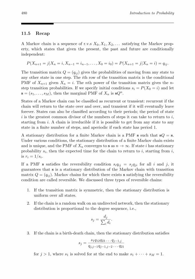
480 Introduction to Probability
11.5 Recap
A Markov chain is a sequence of r.v.s X0
, X1
, X2
, . . . satisfying the Markov prop-erty, which states that given the present, the past and future are conditionallyindependent:
P (Xn+1
= j|Xn = i,Xn�1
= in�1
, . . . , X0
= i0
) = P (Xn+1
= j|Xn = i) = qij .
The transition matrix Q = (qij) gives the probabilities of moving from any state toany other state in one step. The ith row of the transition matrix is the conditionalPMF of Xn+1
given Xn = i. The nth power of the transition matrix gives the n-step transition probabilities. If we specify initial conditions si = P (X
0
= i) and lets = (s
1
, . . . , sM ), then the marginal PMF of Xn is sQn.
States of a Markov chain can be classified as recurrent or transient: recurrent if thechain will return to the state over and over, and transient if it will eventually leaveforever. States can also be classified according to their periods; the period of statei is the greatest common divisor of the numbers of steps it can take to return to i,starting from i. A chain is irreducible if it is possible to get from any state to anystate in a finite number of steps, and aperiodic if each state has period 1.
A stationary distribution for a finite Markov chain is a PMF s such that sQ = s.Under various conditions, the stationary distribution of a finite Markov chain existsand is unique, and the PMF of Xn converges to s as n ! 1. If state i has stationaryprobability si, then the expected time for the chain to return to i, starting from i,is ri = 1/si.
If a PMF s satisfies the reversibility condition siqij = sjqji for all i and j, itguarantees that s is a stationary distribution of the Markov chain with transitionmatrix Q = (qij). Markov chains for which there exists s satisfying the reversibilitycondition are called reversible. We discussed three types of reversible chains:
1. If the transition matrix is symmetric, then the stationary distribution isuniform over all states.
2. If the chain is a random walk on an undirected network, then the stationarydistribution is proportional to the degree sequence, i.e.,
sj =djPi di
.
3. If the chain is a birth-death chain, then the stationary distribution satisfies
sj =s1
q12
q23
. . . qj�1,j
qj,j�1
qj�1,j�2
. . . q21
for j > 1, where s1
is solved for at the end to make s1
+ · · ·+ sM = 1.

Markov chains 481
stationary distribution s for the initial state
distributions random variables events numbers
(given this event, past and future are independent)
generate Pany distribution t for the initial state
generate
X0
, X1
, X2
, . . .
Y0
, Y1
, Y2
, . . .
Xn
= i P (Xn
= i) = (tQn)i
Yn
= i
(given this event, past and future are independent)
PP (Y
n
= i) = si
converges to si
as n ! 1
2 4 6 8 10
0.00
0.05
0.10
0.15
state
pmf
1 2 3 4 5 6 7 8 9 10
What can happen?
FIGURE 11.6
Given a transition matrix Q and a distribution t over the states, we can generatea Markov chain X
0
, X1
, . . . by choosing X0
according to t and then running thechain according to the transition probabilities. An important event is Xn = i, theevent that the chain is visiting state i at time n. We can then find the PMF of Xn
in terms of Q and t, and (under conditions discussed in the chapter) the PMF willconverge to the stationary distribution s. If instead we start the chain out accordingto s, then the chain will stay stationary forever.
Figure 11.6 compares two ways to run a Markov chain with transition matrix Q:choosing the initial state according to an arbitrary distribution t over the states, orchoosing the initial state according to the stationary distribution s. In the formercase, the exact PMF after n steps can be found in terms of Q and t, and the PMFconverges to s (under some very general conditions discussed in this chapter). Inthe latter case, the chain is stationary forever.
11.6 R
Matrix calculations
Let’s do some calculations for the 4-state Markov chain in Example 11.1.5, as anexample of working with transition matrices in R. First, we need to specify thetransition matrix Q. This is done with the matrix command: we type in the entries

482 Introduction to Probability
of the matrix, row by row, as a long vector, and then we tell R the number of rowsand columns in the matrix (nrow and ncol), as well as the fact that we typed inthe entries by row (byrow=TRUE):
Q <- matrix(c(1/3,1/3,1/3,0,
0,0,1/2,1/2,
0,1,0,0,
1/2,0,0,1/2),nrow=4,ncol=4,byrow=TRUE)
To obtain higher order transition probabilities, we can multiply Q by itself repeat-edly. The matrix multiplication command in R is %*% (not just *). So
Q2 <- Q %*% Q
Q3 <- Q2 %*% Q
Q4 <- Q2 %*% Q2
Q5 <- Q3 %*% Q2
produces Q2 through Q5. If we want to know the probability of going from state 3to state 4 in exactly 5 steps, we can extract the (3, 4) entry of Q5:
Q5[3,4]
This gives 0.229, agreeing with the value 11/48 shown in Example 11.1.5.
To compute a power Qn without directly doing repeated matrix multiplications, wecan use the command Q %^% n after installing and loading the expm package. Forexample, Q %^% 42 yields Q42. By exploring the behavior of Qn as n grows, we cansee Theorem 11.3.6 in action (and get a sense of how long it takes for the chain toget very close to its stationary distribution).
In particular, for n large each row of Qn is approximately (0.214, 0.286, 0.214, 0.286),so this is approximately the stationary distribution. Another way to obtain thestationary distribution numerically is to use
eigen(t(Q))
to compute the eigenvalues and eigenvectors of the transpose of Q; then the eigen-vector corresponding to the eigenvalue 1 can be selected and normalized so that thecomponents sum to 1.
Gambler’s ruin
To simulate from the gambler’s ruin chain, we start by deciding the total amountof money N between the two gamblers, the probability p of gambler A winning agiven round, and the number of time periods nsim that we wish to simulate.
N <- 10
p <- 1/2
nsim <- 80

Markov chains 483
Next, we allocate a vector of length nsim called x, which will store the values of theMarkov chain. For the initial condition, we set the first entry of x equal to 5; thisgives both gamblers $5 to start with.
x <- rep(0,nsim)
x[1] <- 5
Now we are ready to simulate the subsequent values of the Markov chain. This isachieved with the following block of code, which we will explain step by step.
for (i in 2:nsim){
if (x[i-1]==0 || x[i-1]==N){
x[i] <- x[i-1]
}
else{
x[i] <- x[i-1] + sample(c(1,-1), 1, prob=c(p,1-p))
}
}
The first line and the outer set of braces constitute a for loop: for (i in 2:nsim)
means that all the code inside the for loop will be executed over and over, with thevalue of i set to 2, then set to 3, then set to 4, all the way until i reaches the valuensim. Each pass through the loop represents one step of the Markov chain.
Inside the for loop, we first check to see whether the chain is already at one of theendpoints, 0 or N; we do this with an if statement. If the chain is already at 0 or N,then we set its new value equal to its previous value, since the chain is not allowedto escape 0 or N. Otherwise, if the chain is not at 0 or N, it is free to move left orright. We use the sample command to move to the right 1 unit or to the left 1 unit,with probabilities p and 1-p, respectively.
To see what path was taken by the Markov chain during our simulation, we canplot the values of x as a function of time:
plot(x,type=‘l’,ylim=c(0,N))
You should see a path that starts at 5 and bounces up and down before beingabsorbed into state 0 or state N.
Simulating from a finite-state Markov chain
With a few modifications, we can simulate from an arbitrary Markov chain on afinite state space. For concreteness, we will illustrate how to simulate from the4-state Markov chain in Example 11.1.5.
As above, we can type
Q <- matrix(c(1/3,1/3,1/3,0,
0,0,1/2,1/2,

484 Introduction to Probability
0,1,0,0,
1/2,0,0,1/2),nrow=4,ncol=4,byrow=TRUE)
to specify the transition matrix Q.
Next, we choose the number of states and the number of time periods to simulate,we allocate space for the results of the simulation, and we choose initial conditionsfor the chain. In this example, x[1] <- sample(1:M,1) says the initial distributionof the chain is uniform over all states.
M <- nrow(Q)
nsim <- 10^4
x <- rep(0,nsim)
x[1] <- sample(1:M,1)
For the simulation itself, we again use sample to choose a number from 1 to M.At time i, the chain was previously at state x[i-1], so we must use row x[i-1]
of the transition matrix to determine the probabilities of sampling 1, 2, . . . , M. Thenotation Q[x[i-1],] denotes row x[i-1] of the matrix Q.
for (i in 2:nsim){
x[i] <- sample(M, 1, prob=Q[x[i-1],])
}
Since we set nsim to a large number, it may be reasonable to believe that thechain is close to stationarity during the latter portion of the simulation. To checkthis, we eliminate the first half of the simulations to give the chain time to reachstationarity:
x <- x[-(1:(nsim/2))]
We then use the table command to calculate the number of times the chain visitedeach state; dividing by length(x) converts the counts into proportions. The resultis an approximation to the stationary distribution.
table(x)/length(x)
For comparison, the true stationary distribution of the chain is (3/14, 2/7, 3/14, 2/7) ⇡(0.214, 0.286, 0.214, 0.286). Is this close to what you obtained empirically?
11.7 Exercises
Markov property
1. s� LetX0
, X1
, X2
, . . . be a Markov chain. Show thatX0
, X2
, X4
, X6
, . . . is also a Markovchain, and explain why this makes sense intuitively.
2. s� Let X0
, X1
, X2
, . . . be an irreducible Markov chain with state space {1, 2, . . . ,M},

Markov chains 485
M � 3, transition matrix Q = (qij), and stationary distribution s = (s1
, . . . , sM ). Letthe initial state X
0
follow the stationary distribution, i.e., P (X0
= i) = si.
(a) On average, how many of X0
, X1
, . . . , X9
equal 3? (In terms of s; simplify.)
(b) Let Yn = (Xn�1)(Xn�2). For M = 3, find an example of Q (the transition matrixfor the original chain X
0
, X1
, . . . ) where Y0
, Y1
, . . . is Markov, and another example ofQ where Y
0
, Y1
, . . . is not Markov. In your examples, make qii > 0 for at least one i andmake sure it is possible to get from any state to any other state eventually.
3. A Markov chain has two states, A and B, with transitions as follows:
BA
0.5
0.51
Suppose we do not get to observe this Markov chain, which we’ll call X0
, X1
, X2
, . . . .Instead, whenever the chain transitions from A back to A, we observe a 0, and wheneverit changes states, we observe a 1. Let the sequence of 0’s and 1’s be called Y
0
, Y1
, Y2
, . . . .
For example, if the X chain starts out as
A,A,B,A,B,A,A, . . .
then the Y chain starts out as0, 1, 1, 1, 1, 0, . . .
(a) Show that Y0
, Y1
, Y2
, . . . is not a Markov chain.
(b) In Example 11.1.3, we dealt with a violation of the Markov property by enlargingthe state space to incorporate second-order dependence. Show that such a trick will notwork for Y
0
, Y1
, Y2
. . . . That is, no matter how large m is,
Zn = {the (n�m+ 1)st to nth terms of the Y chain}
is still not a Markov chain.
Stationary distribution
4. s� Consider the Markov chain shown below, where 0 < p < 1 and the labels on thearrows indicate transition probabilities.
1
p
21-p
1-p
p
(a) Write down the transition matrix Q for this chain.
(b) Find the stationary distribution of the chain.
(c) What is the limit of Qn as n ! 1?

486 Introduction to Probability
1 0.5
2
0.5 0.25
0.75
3 0.25
4
0.75 0.75
0.25
5. s� Consider the Markov chain shown below, with state space {1, 2, 3, 4} and the labelson the arrows indicate transition probabilities.
(a) Write down the transition matrix Q for this chain.
(b) Which states (if any) are recurrent? Which states (if any) are transient?
(c) Find two di↵erent stationary distributions for the chain.
6. s� Daenerys has three dragons: Drogon, Rhaegal, and Viserion. Each dragon indepen-dently explores the world in search of tasty morsels. Let Xn, Yn, Zn be the locations attime n of Drogon, Rhaegal, Viserion respectively, where time is assumed to be discreteand the number of possible locations is a finite number M . Their paths X
0
, X1
, X2
, . . . ;Y0
, Y1
, Y2
, . . . ; and Z0
, Z1
, Z2
, . . . are independent Markov chains with the same station-ary distribution s. Each dragon starts out at a random location generated according tothe stationary distribution.
(a) Let state 0 be home (so s0
is the stationary probability of the home state). Findthe expected number of times that Drogon is at home, up to time 24, i.e., the expectednumber of how many of X
0
, X1
, . . . , X24
are state 0 (in terms of s0
).
(b) If we want to track all 3 dragons simultaneously, we need to consider the vectorof positions, (Xn, Yn, Zn). There are M3 possible values for this vector; assume thateach is assigned a number from 1 to M3, e.g., if M = 2 we could encode the states(0, 0, 0), (0, 0, 1), (0, 1, 0), . . . , (1, 1, 1) as 1, 2, 3, . . . , 8 respectively. Let Wn be the num-ber between 1 and M3 representing (Xn, Yn, Zn). Determine whether W
0
,W1
, . . . is aMarkov chain.
(c) Given that all 3 dragons start at home at time 0, find the expected time it will takefor all 3 to be at home again at the same time.
Reversibility
7. s� A Markov chain X0
, X1
, . . . with state space {�3,�2,�1, 0, 1, 2, 3} proceeds as fol-lows. The chain starts at X
0
= 0. If Xn is not an endpoint (�3 or 3), then Xn+1
isXn � 1 or Xn +1, each with probability 1/2. Otherwise, the chain gets reflected o↵ theendpoint, i.e., from 3 it always goes to 2 and from �3 it always goes to �2. A diagramof the chain is shown below.
-3 -2 -1 0 1 2 3
(a) Is |X0
|, |X1
|, |X2
|, . . . also a Markov chain? Explain.
Hint: For both (a) and (b), think about whether the past and future are conditionallyindependent given the present; don’t do calculations with a 7 by 7 transition matrix!

Markov chains 487
(b) Let sgn be the sign function: sgn(x) = 1 if x > 0, sgn(x) = �1 if x < 0, andsgn(0) = 0. Is sgn(X
0
), sgn(X1
), sgn(X2
), . . . a Markov chain? Explain.
(c) Find the stationary distribution of the chain X0
, X1
, X2
, . . . .
(d) Find a simple way to modify some of the transition probabilities qij for i 2 {�3, 3}to make the stationary distribution of the modified chain uniform over the states.
8. s� Let G be an undirected network with nodes labeled 1, 2, . . . ,M (edges from a nodeto itself are not allowed), where M � 2 and random walk on this network is irreducible.Let dj be the degree of node j for each j. Create a Markov chain on the state space1, 2, . . . ,M , with transitions as follows. From state i, generate a proposal j by choosinga uniformly random j such that there is an edge between i and j in G; then go to jwith probability min(di/dj , 1), and stay at i otherwise.
(a) Find the transition probability qij from i to j for this chain, for all states i, j.
(b) Find the stationary distribution of this chain.
9. s� (a) Consider a Markov chain on the state space {1, 2, . . . , 7} with the states arrangedin a “circle” as shown below, and transitions given by moving one step clockwise orcounterclockwise with equal probabilities. For example, from state 6, the chain movesto state 7 or state 5 with probability 1/2 each; from state 7, the chain moves to state 1or state 6 with probability 1/2 each. The chain starts at state 1.
1
2
3
4
5
6
7
Find the stationary distribution of this chain.
(b) Consider a new chain obtained by “unfolding the circle.” Now the states are arrangedas shown below. From state 1 the chain always goes to state 2, and from state 7 thechain always goes to state 6. Find the new stationary distribution.
1 2 3 4 5 6 7
10. s� Let Xn be the price of a certain stock at the start of the nth day, and assume thatX
0
, X1
, X2
, . . . follows a Markov chain with transition matrix Q. (Assume for simplicitythat the stock price can never go below 0 or above a certain upper bound, and that itis always rounded to the nearest dollar.)
s� (a) A lazy investor only looks at the stock once a year, observing the values on days0, 365, 2 · 365, 3 · 365, . . . . So the investor observes Y
0
, Y1
, . . . , where Yn is the price aftern years (which is 365n days; you can ignore leap years). Is Y
0
, Y1
, . . . also a Markovchain? Explain why or why not; if so, what is its transition matrix?
(b) The stock price is always an integer between $0 and $28. From each day to the next,

488 Introduction to Probability
the stock goes up or down by $1 or $2, all with equal probabilities (except for days whenthe stock is at or near a boundary, i.e., at $0, $1, $27, or $28).
If the stock is at $0, it goes up to $1 or $2 on the next day (after receiving governmentbailout money). If the stock is at $28, it goes down to $27 or $26 the next day. If thestock is at $1, it either goes up to $2 or $3, or down to $0 (with equal probabilities);similarly, if the stock is at $27 it either goes up to $28, or down to $26 or $25. Find thestationary distribution of the chain.
11. s� In chess, the king can move one square at a time in any direction (horizontally,vertically, or diagonally).
For example, in the diagram, from the current position the king can move to any of 8possible squares. A king is wandering around on an otherwise empty 8⇥ 8 chessboard,where for each move all possibilities are equally likely. Find the stationary distributionof this chain (of course, don’t list out a vector of length 64 explicitly! Classify the 64squares into types and say what the stationary probability is for a square of each type).
12. A chess piece is wandering around on an otherwise vacant 8 ⇥ 8 chessboard. At eachmove, the piece (a king, queen, rook, bishop, or knight) chooses uniformly at randomwhere to go, among the legal choices (according to the rules of chess, which you shouldlook up if you are unfamiliar with them).
(a) For each of these cases, determine whether the Markov chain is irreducible, andwhether it is aperiodic.
Hint for the knight: Note that a knight’s move always goes from a light square to a darksquare or vice versa. A knight’s tour is a sequence of knight moves on a chessboard suchthat the knight visits each square exactly once. Many knight’s tours exist.
(b) Suppose for this part that the piece is a rook, with initial position chosen uniformlyat random. Find the distribution of where the rook is after n moves.
(c) Now suppose that the piece is a king, with initial position chosen deterministicallyto be the upper left corner square. Determine the expected number of moves it takeshim to return to that square, fully simplified, preferably in at most 140 characters.
(d) The stationary distribution for the random walk of the king from the previous partis not uniform over the 64 squares of the chessboard. A recipe for modifying the chain toobtain a uniform stationary distribution is as follows. Label the squares as 1, 2, . . . , 64,and let di be the number of legal moves from square i. Suppose the king is currently atsquare i. The next move of the chain is determined as follows:
Step 1: Generate a proposal square j by picking uniformly at random among the legalmoves from i.

Markov chains 489
Step 2: Flip a coin with probability min(di/dj , 1) of Heads. If the coin lands Heads, goto j. Otherwise, stay at i.
Show that this modified chain has a stationary distribution that is uniform over the 64squares.
13. s� Find the stationary distribution of the Markov chain shown below, without usingmatrices. The number above each arrow is the corresponding transition probability.
1 211/2
31/21/4
5/12
41/31/6
7/12
51/41/8
7/8
14. There are two urns with a total of 2N distinguishable balls. Initially, the first urn hasN white balls and the second urn has N black balls. At each stage, we pick a ball atrandom from each urn and interchange them. Let Xn be the number of black balls inthe first urn at time n. This is a Markov chain on the state space {0, 1, . . . , N}.
(a) Give the transition probabilities of the chain.
(b) Show that (s0
, s1
, . . . , sN ) where
si =
�Ni
��N
N�i
��2NN
�
is the stationary distribution, by verifying the reversibility condition.
15. Nausicaa Distribution sells distribution plushies on Etsy. They have two di↵erent photosof the Evil Cauchy plushie but do not know which is more e↵ective in getting a customerto purchase an Evil Cauchy plushie. Each visitor to their website is shown one of thetwo photos (call them Photo A and Photo B), and then the visitor either does buy anEvil Cauchy (“success”) or does not buy one (“failure”).
Let a and b be the probabilities of success when Photo A is shown and when Photo B isshown, respectively. Even though the Evil Cauchy is irresistible, suppose that 0 < a < 1and 0 < b < 1. Suppose that the following strategy is followed (note that the strategycan be followed without knowing a and b). Show the first visitor Photo A. If that visitorbuys an Evil Cauchy, continue with Photo A for the next visitor; otherwise, switch toPhoto B. Similarly, if the nth visitor is a “success” then show the (n+ 1)st visitor thesame photo, and otherwise switch to the other photo.
(a) Show how to represent the resulting process as a Markov chain, drawing a diagramand giving the transition matrix. The states are A1, B1, A0, B0 (use this order for thetransition matrix and stationary distribution), where, for example, being at state A1means that the current visitor was shown Photo A and was a success.
(b) Determine whether this chain is reversible.
Hint: First think about which transition probabilities are zero and which are nonzero.
(c) Show that the stationary distribution is proportional to⇣
a1�a
, b1�b
, 1, 1⌘, and find
the stationary distribution.
(d) Show that for a 6= b, the stationary probability of success for each visitor is strictlybetter than the success probability that would be obtained by independently, randomlychoosing (with equal probabilities) which photo to show to each visitor.

490 Introduction to Probability
16. This exercises considers random walk on a weighted undirected network. Suppose thatan undirected network is given, where each edge (i, j) has a nonnegative weight wij
assigned to it (we allow i = j as a possibility). We assume that wij = wji since the edgefrom i to j is considered the same as the edge from j to i. To simplify notation, definewij = 0 whenever (i, j) is not an edge.
When at node i, the next step is determined by choosing an edge attached to i withprobabilities proportional to the weights. For example, if the walk is at node 1 and thereare 3 possible edges coming out from node 1, with weights 7, 1, 4, then the first of these 3edges is traversed with probability 7/12, the second is traversed with probability 1/12,and the third is traversed with probability 4/12. If all the weights equal 1, then theprocess reduces to the kind of random walk on a network that we studied earlier.
(a) Let vi =P
j wij for all nodes i. Show that the stationary distribution of node i isproportional to vi.
(b) Show that every reversible Markov chain can be represented as a random walk on aweighted undirected network.
Hint: Let wij = siqij , where s is the stationary distribution and qij is the transitionprobability from i to j.
Mixed practice
17. s� A cat and a mouse move independently back and forth between two rooms. At eachtime step, the cat moves from the current room to the other room with probability 0.8.Starting from room 1, the mouse moves to Room 2 with probability 0.3 (and remainsotherwise). Starting from room 2, the mouse moves to room 1 with probability 0.6 (andremains otherwise).
(a) Find the stationary distributions of the cat chain and of the mouse chain.
(b) Note that there are 4 possible (cat, mouse) states: both in room 1, cat in room1 and mouse in room 2, cat in room 2 and mouse in room 1, and both in room 2.Number these cases 1, 2, 3, 4, respectively, and let Zn be the number representing the(cat, mouse) state at time n. Is Z
0
, Z1
, Z2
, . . . a Markov chain?
(c) Now suppose that the cat will eat the mouse if they are in the same room. We wishto know the expected time (number of steps taken) until the cat eats the mouse for twoinitial configurations: when the cat starts in room 1 and the mouse starts in room 2,and vice versa. Set up a system of two linear equations in two unknowns whose solutionis the desired values.
18. Let {Xn} be a Markov chain on states {0, 1, 2} with transition matrix
0
BBBBB@
0.8 0.2 0
0 0.8 0.2
0 0 1
1
CCCCCA
The chain starts at X0
= 0. Let T be the time it takes to reach state 2:
T = min{n : Xn = 2}.
By drawing the Markov chain and telling a story, find E(T ) and Var(T ).
19. Consider the following Markov chain on the state space {1, 2, 3, 4, 5, 6}.

Markov chains 491
4
6
3
5
21
0.5
0.50.5
0.5
0.3
0.2 0.2 0.7 0.7
0.30.8
0.50.3
(a) Suppose the chain starts at state 1. Find the distribution of the number of timesthat the chain returns to state 1.
(b) In the long run, what fraction of the time does the chain spend in state 3? Explainbriefly.
20. Let Q be the transition matrix of a Markov chain on the state space {1, 2, . . . ,M}, suchthat state M is an absorbing state, i.e., from state M the chain can never leave. Supposethat from any other state, it is possible to reach M (in some number of steps).
(a) Which states are recurrent, and which are transient? Explain.
(b) What is the limit of Qn as n ! 1?
(c) For i, j 2 {1, 2, . . . ,M � 1}, find the probability that the chain is at state j at timen, given that the chain is at state i at time 0 (your answer should be in terms of Q).
(d) For i, j 2 {1, 2, . . . ,M � 1}, find the expected number of times that the chain is atstate j up to (and including) time n, given that the chain is at state i at time 0 (interms of Q).
(e) Let R be the (M�1)⇥ (M�1) matrix obtained from Q by deleting the last row andthe last column of Q. Show that the (i, j) entry of (I �R)�1 is the expected number oftimes that the chain is at state j before absorption, given that it starts out at state i.
Hint: We have I +R+R2 + · · · = (I �R)�1, analogously to a geometric series. Also, ifwe partition Q as
Q =
0
B@R B
0 1
1
CA
where B is a (M � 1)⇥ 1 matrix and 0 is the 1⇥ (M � 1) zero matrix, then
Qk =
0
B@Rk Bk
0 1
1
CA
for some (M � 1)⇥ 1 matrix Bk.

492 Introduction to Probability
21. In the game called Chutes and Ladders, players try to be first to reach a certain desti-nation on a board. The board is a grid of squares, numbered from 1 to the number ofsquares. The board has some “chutes” and some “ladders”, each of which connects apair of squares. Here we will consider the one player version of the game (this can be ex-tended to the multi-player version without too much trouble, since with more than oneplayer, the players simply take turns independently until one reaches the destination).
On each turn, the player rolls a fair die, which determines how many squares forward tomove on the grid, e.g., if the player is at square 5 and rolls a 3, then he or she advancesto square 8. If the resulting square is the base of a ladder, the player gets to climb theladder, instantly arriving at a more advanced square. If the resulting square is the topof a chute, the player instantly slides down to the bottom of the chute.
This game can be viewed naturally as a Markov chain: given where the player currentlyis on the board, the past history does not matter for computing, for example, theprobability of winning within the next 3 moves.
Consider a simplified version of Chutes and Ladders, played on the 3⇥ 3 board shownbelow. The player starts out at square 1, and wants to get to square 9. On each move, afair coin is flipped, and the player gets to advance 1 square if the coin lands Heads and 2squares if the coin lands Tails. However, there are 2 ladders (shown as upward-pointingarrows) and 2 chutes (shown as downward-pointing arrows) on the board.
7 8 9
6 5 4
1 2 3
(a) Explain why, despite the fact that there are 9 squares, we can represent the gameusing the 5⇥ 5 transition matrix
Q =
0
BBBBBBBBBBBB@
0 0.5 0.5 0 0
0 0 0.5 0.5 0
0.5 0 0 0.5 0
0.5 0 0 0 0.5
0 0 0 0 1
1
CCCCCCCCCCCCA
.
(b) Find the mean and variance for the number of times the player will visit square 7,without using matrices or any messy calculations.
The remaining parts of this problem require matrix calculations that are best done ona computer. You can use whatever computing environment you want, but here is someinformation for how to do it in R. In any case, you should state what environmentyou used and include your code. To create the transition matrix in R, you can use thefollowing commands:

Markov chains 493
a <- 0.5
Q <- matrix(c(0,0,a,a,0,a,0,0,0,0,a,a,0,0,0,0,a,a,0,0,0,0,0,a,1),nrow=5)
Some useful R commands for matrices are in Appendix B.2. In particular, diag(n) givesthe n⇥n identity matrix, solve(A) gives the inverse A�1, and A %*% B gives the productAB (note that A*B does not do ordinary matrix multiplication). Matrix powers are notbuilt into R, but you can compute Ak using A %^% k after installing and loading theexpm package.
(c) Find the median duration of the game (defining duration as the number of coinflips).
Hint: Relate the CDF of the duration to powers of Q.
(d) Find the mean duration of the game (with duration defined as above).
Hint: Relate the duration to the total amount of time spent in transient states, andapply Part (e) of the previous problem.


12
Markov chain Monte Carlo
We have seen throughout this book that simulation is a powerful technique inprobability. If you can’t convince your friend that it is a good idea to switch doorsin the Monty Hall problem, in one second you can simulate playing the game afew thousand times and your friend will just see that switching succeeds about 2/3of the time. If you’re unsure how to calculate the mean and variance of an r.v. Xbut you know how to generate i.i.d. draws X
1
, X2
, . . . , Xn from that distribution,you can approximate the true mean and true variance using the sample mean andsample variance of the simulated draws:
E(X) ⇡ 1
n(X
1
+ · · ·+Xn) = Xn,
Var(X) ⇡ 1
n� 1
nX
j=1
(Xj � Xn)2.
The law of large numbers tells us that these approximations will be good if nis large. We can get better and better approximations by increasing n, just byrunning the computer for a longer time (rather than having to struggle with apossibly intractable sum or integral). As discussed in Chapter 10, this simulationapproach, where we generate random values to approximate a quantity, is called aMonte Carlo method.
A major limitation of the Monte Carlo idea above is that we need to know howto generate X
1
, X2
, . . . , Xn (hopefully e�ciently, since we want to be able to maken large). For example, suppose that we want to simulate random draws from thecontinuous distribution with PDF f given by
f(x) / x3.1(1� x)4.2
for 0 < x < 1 (and 0 otherwise). Staring at a density function does not immediatelysuggest how to get a random variable with that density. In this case we recognizethe PDF of the Beta(4.1, 5.2) distribution, so assuming we had access to a Unif(0, 1)r.v., we could theoretically use universality of the Uniform. Unfortunately, findingthe CDF of a Beta distribution is di�cult, let alone the inverse of the CDF. SeeExample 12.1.4 for more about the Beta simulation problem.
Of course, the distributions that arise in real-world applications are often muchmore complicated than the Beta. For the Beta distribution, we know an expressionfor the normalizing constant in terms of the gamma function. But for many other
495

496 Introduction to Probability
distributions that are of scientific interest, the normalizing constant in the PDFor PMF is unknown, beyond the reach of the fastest available computers and thefanciest available mathematical techniques.
This chapter introduces Markov chain Monte Carlo (MCMC), a powerful collec-tion of algorithms that enable us to simulate from complicated distributions usingMarkov chains. The development of MCMC has revolutionized statistics and scien-tific computation by vastly expanding the range of possible distributions that wecan simulate from, including joint distributions in high dimensions. The basic idea isto build your own Markov chain so that the distribution of interest is the stationarydistribution of the chain.
In the previous chapter, we looked at Markov chains whose transition matrix Qwas specified, and we tried to find the stationary distribution s of the chain. In thischapter we do the reverse: starting with a distribution s that we want to simulate,we will engineer a Markov chain whose stationary distribution is s. If we then runthis engineered Markov chain for a very long time, the distribution of the chain willapproach our desired s.
But is it possible to create a transition matrix Q with the stationary distributionwe desire? Even if it is possible, is solving this problem any easier than the origi-nal problem of how to simulate random draws from that distribution? In amazinggenerality, MCMC shows that it is possible to create a Markov chain with the de-sired stationary distribution in an easy-to-describe way, without having to know thenormalizing constant for the distribution!
MCMC is now being applied to a large number of problems in the biological, natural,and physical sciences, and many di↵erent MCMC algorithms have been developed.Here we will introduce two of the most important and most widely used MCMCalgorithms: the Metropolis-Hastings algorithm and Gibbs sampling. MCMC is anenormous and growing area of statistical computing; see Brooks, Gelman, Jones,and Meng [2] for much more about its theory, methods, and applications.
12.1 Metropolis-Hastings
The Metropolis-Hastings algorithm is a general recipe that lets us start with anyirreducible Markov chain on the state space of interest and then modify it into anew Markov chain that has the desired stationary distribution. This modificationconsists of introducing some selectiveness in the original chain: moves are proposedaccording to the original chain, but the proposal may or may not be accepted. Forexample, suppose the original chain is at a state called “Boston” and is about totransition to “San Francisco”. Then for the new chain, we either accept the proposaland go to San Francisco, or we turn down the proposal and remain in Boston as

Markov chain Monte Carlo 497
the next step. With a careful choice of the probability of accepting the proposal,this simple modification guarantees that the new chain has the desired stationarydistribution.
Algorithm 12.1.1 (Metropolis-Hastings). Let s = (s1
, . . . , sM ) be a desired sta-tionary distribution on state space {1, . . . ,M}. Assume that si > 0 for all i (if not,just delete any states i with si = 0 from the state space). Suppose that P = (pij)is the transition matrix for a Markov chain on state space {1, . . . ,M}. Intuitively,P is a Markov chain that we know how to run but that doesn’t have the desiredstationary distribution.
Our goal is to modify P to construct a Markov chain X0
, X1
, . . . with stationarydistribution s. We will give a Metropolis-Hastings algorithm for this. Start at anystate X
0
(chosen randomly or deterministically), and suppose that the new chain iscurrently at Xn. To make one move of the new chain, do the following.
1. If Xn = i, propose a new state j using the transition probabilities inthe ith row of the original transition matrix P .
2. Compute the acceptance probability
aij = min
✓sjpjisipij
, 1
◆.
3. Flip a coin that lands Heads with probability aij .
4. If the coin lands Heads, accept the proposal (i.e., go to j), settingXn+1
= j. Otherwise, reject the proposal (i.e., stay at i), setting Xn+1
= i.
That is, the Metropolis-Hastings chain uses the original transition probabilities pijto propose where to go next, then accepts the proposal with probability aij , stayingin its current state in the event of a rejection. An especially nice aspect of thisalgorithm is that the normalizing constant for s does not need to be known, since itcancels out in sj/si anyway. For example, in some problems we may want the sta-tionary distribution to be uniform over all states (i.e., s = (1/M, 1/M, . . . , 1/M)),but the number of states M is large and unknown, and it would be a very hardcounting problem to find M . Fortunately, sj/si = 1 regardless of M , so we can sim-ply say s / (1, 1, . . . , 1), and we can calculate aij without having to know M .
The pij in the denominator in aij will never be 0 when the algorithm is run, since ifpij = 0 then the original chain will never propose going from i to j. Also, if pii > 0 itis possible that the proposal j will equal the current state i; in that case, the chainstays at i regardless of whether the proposal is accepted. (Rejecting the proposal ofstaying at i but staying there anyway is like a child who just got grounded saying“yes, I will stay in my room, but not because you told me to!”)
We will now show that the Metropolis-Hastings chain is reversible with stationarydistribution s.

498 Introduction to Probability
Proof. Let Q be the transition matrix of the Metropolis-Hastings chain. We justneed to check the reversibility condition siqij = sjqji for all i and j. This is clearfor i = j, so assume i 6= j. If qij > 0, then pij > 0 (the chain can’t get from i toj if it can’t even propose going from i to j) and pji > 0 (otherwise the acceptanceprobability would be 0). Conversely, if pij > 0 and pji > 0, then qji > 0. So qij andqji are either both zero or both nonzero. We can assume they are both nonzero.Then
qij = pijaij
since, starting at i, the only way to get to j is first to propose doing so and then toaccept the proposal. First consider the case sjpji sipij . We have
aij =sjpjisipij
, aji = 1,
sosiqij = sipijaij = sipij
sjpjisipij
= sjpji = sjpjiaji = sjqji.
Symmetrically, if sjpji > sipij , we again have siqij = sjqji, by switching the rolesof i and j in the preceding calculation. Since the reversibility condition holds, s isthe stationary distribution of the chain with transition matrix Q. ⌅h 12.1.2. The Metropolis-Hastings algorithm is an extremely general way to con-struct a Markov chain with a desired stationary distribution. In the above formula-tion, both s and P were very general, and nothing was stipulated about their beingrelated (aside from being on the same state space). In practice, however, the choiceof the proposal distribution is extremely important since it can make an enormousdi↵erence in how fast the chain converges to its stationary distribution.
How to choose a good proposal distribution is a complicated topic and will notbe discussed in detail here. Intuitively, a proposal distribution with a very lowacceptance rate will be slow to converge (since the chain will rarely move anywhere).But a high acceptance rate may not be ideal either, since it may indicate that thechain tends to make small, timid proposals. In a large state space, such a chain willtake a very long time to explore the entire space.
Here are a couple examples of how the Metropolis-Hastings algorithm can be usedto simulate from distributions.
Example 12.1.3 (Zipf distribution simulation). Let M � 2 be an integer. Anr.v. X has the Zipf distribution with parameter a > 0 if its PMF is
P (X = k) =1/ka
PMj=1
(1/ja),
for k = 1, 2, . . . ,M (and 0 otherwise). This distribution is widely used in linguisticsfor studying frequencies of words.
Create a Markov chain X0
, X1
, . . . whose stationary distribution is the Zipf distri-bution, and such that |Xn+1
� Xn| 1 for all n. Your answer should provide a

Markov chain Monte Carlo 499
simple, precise description of how each move of the chain is obtained, i.e., how totransition from Xn to Xn+1
for each n.
Solution:
We can use the Metropolis-Hastings algorithm, after coming up with a proposaldistribution. There are many possible proposal distributions, but one simple choiceis the following random walk on {1, 2, . . . ,M}. From state i with i 6= 1, i 6= M ,move to state i� 1 or i+ 1, with probability 1/2 each. From state 1, stay there ormove to state 2, with probability 1/2 each. From state M , stay there or move tostate M � 1, with probability 1/2 each.
1 32 MM – 1...
FIGURE 12.1
Proposal chain for Zipf distribution simulation.
Let P be the transition matrix of this chain. The stationary distribution for P isuniform because P is a symmetric matrix, so Proposition 11.4.3 applies. Metropolis-Hastings lets us transmogrify P into a chain whose stationary distribution is Zipf’sdistribution.
Let X0
be any starting state, and generate a chain X0
, X1
, . . . as follows. If thechain is currently at state i, then:
1. Generate a proposal state j according to the proposal chain P .
2. Accept the proposal with probability min (ia/ja, 1). If the proposal isaccepted, go to j; otherwise, stay at i.
This chain is easy to implement and a move requires very little computation; notethat the normalizing constant
PMj=1
(1/ja) is not needed to run the chain. ⇤Example 12.1.4 (Beta simulation). Let us now return to the Beta simulation prob-lem introduced at the beginning of the chapter. Suppose that we want to generateW ⇠ Beta(a, b), but we don’t know about the rbeta command in R. Instead, whatwe have available are i.i.d. Unif(0, 1) r.v.s.
(a) How can we generate W exactly if a and b are positive integers, using a storyand universality of the Uniform?
(b) How can we generate W which is approximately Beta(a, b) if a and b are anypositive real numbers, with the help of a Markov chain on the continuous statespace (0, 1)?
Solution:
(a) Applying universality of the Uniform directly for the Beta is hard, so let’s firstuse the bank–post o�ce story, which says that if X ⇠ Gamma(a, 1) and Y ⇠

500 Introduction to Probability
Gamma(b, 1) are independent, then X/(X + Y ) ⇠ Beta(a, b). So if we can simulatethe Gamma distribution, then we can simulate the Beta distribution!
To simulate X ⇠ Gamma(a, 1), we can use X1
+ X2
+ · · · + Xa with the Xj
i.i.d. Expo(1); similarly, we can simulate Y ⇠ Gamma(b, 1) as the sum of bi.i.d. Expo(1) r.v.s. Lastly, by taking the inverse of the Expo(1) CDF and applyinguniversality of the Uniform,
� log(1� U) ⇠ Expo(1)
for U ⇠ Unif(0, 1), so we can easily construct as many Expo(1) r.v.s as we want.
(b) Let’s use the Metropolis-Hastings algorithm. We have only introducedMetropolis-Hastings for finite state spaces, but the ideas are analogous for an un-countable state space. A simple proposal chain we have available consists of indepen-dent Unif(0, 1) r.v.s (note that an i.i.d. sequence does satisfy the Markov property).That is, the proposed state on the interval (0, 1) is always a fresh Unif(0, 1), inde-pendent of the current state. The resulting Metropolis-Hastings chain is called anindependence sampler.
Let W0
be any starting state, and generate a chain W0
,W1
, . . . as follows. If thechain is currently at state w (a real number in (0, 1)), then:
1. Generate a proposal u by drawing a Unif(0, 1) r.v.
2. Accept the proposal with probability min⇣
ua�1
(1�u)b�1
wa�1
(1�w)
b�1
, 1⌘. If the pro-
posal is accepted, go to u; otherwise, stay at w.
Again, the normalizing constant was not needed in order to run the chain. In ob-taining the acceptance probability, the Beta(a, b) PDF plays the role of s since it’sthe desired stationary distribution, and the Unif(0, 1) PDF plays the role of pij (andpji) since the proposals are Unif(0, 1) r.v.s, independent of the current state.
Running the Markov chain, we have that Wn,Wn+1
,Wn+2
, . . . are approximatelyBeta(a, b) for n large. Note that these are correlated r.v.s., not i.i.d. draws. ⇤h 12.1.5 (MCMC produces correlated samples). A major question in running aMarkov chain X
0
, X1
, . . . for a Monte Carlo computation is how long to run it. Inpart, this is because it is usually hard to know how close the chain’s distributionat time n will be to the stationary distribution. Another issue is that X
0
, X1
, . . .are correlated in general. Some chains tend to get stuck in certain regions of thestate space, rather than exploring the whole space. If a chain can get stuck easily,then Xn may be highly positively correlated with Xn+1
. The autocorrelation at lagk is the correlation between Xn and the value k steps later, Xn+k, in the limit asn grows. It is desirable for the autocorrelation at lag k to approach 0 rapidly ask increases. High autocorrelation generally means high variances for Monte Carloapproximations.
Analysis of how long to run a chain and finding diagnostics for whether the chain

Markov chain Monte Carlo 501
has been run long enough are active research areas. Some general advice is to runyour chains for a very large number of steps and to try chains from diverse startingpoints to see how stable the results are.
Metropolis-Hastings is often useful even for immense state spaces. It can even beuseful for problems that may not sound at first like they have anything to do withsimulating a distribution, such as code-breaking.
Example 12.1.6 (Code-breaking). Markov chains have recently been applied tocode-breaking; this example will introduce one way in which this can be done.(For further information about such applications, see Diaconis [7] and Chen andRosenthal [4].) A substitution cipher is a permutation g of the letters from a to z,where a message is enciphered by replacing each letter ↵ by g(↵). For example, if gis the permutation given by
abcdefghijklmnopqrstuvwxyz
zyxwvutsrqponmlkjihgfedcba
where the second row lists the values g(a), g(b), . . . , g(z), then we would encipherthe word “statistics” as “hgzgrhgrxh”. (We could also include capital letters, spaces,and punctuation marks if desired.) The state space is all 26! ⇡ 4 ·1026 permutationsof the letters a through z. This is an extremely large space: if we had to try de-coding a text using each of these permutations, and could handle one permutationper nanosecond, it would still take over 12 billion years to work through all thepermutations. So a brute-force investigation that goes through each permutationone by one is infeasible; instead, we will look at random permutations.
(a) Consider the Markov chain that picks two di↵erent random coordinates between1 and 26 and swaps those entries of the 2nd row, e.g., if we pick 7 and 20, then
abcdefghijklmnopqrstuvwxyz
zyxwvutsrqponmlkjihgfedcba
becomes
abcdefghijklmnopqrstuvwxyz
zyxwvugsrqponmlkjihtfedcba
Find the probability of going from a permutation g to a permutation h in one step(for all g, h), and find the stationary distribution of this chain.
(b) Suppose we have a system that assigns a positive “score” s(g) to each permu-tation g. Intuitively, this could be a measure of how likely it would be to get theobserved enciphered text, given that g was the cipher used. Use the Metropolis-Hastings algorithm to construct a Markov chain whose stationary distribution isproportional to the list of all scores s(g).
Solution:
(a) The probability of going from g to h in one step is 0 unless h can be obtained

502 Introduction to Probability
from g by swapping 2 entries of the second row. Assuming that h can be obtainedin this way, the probability is 1
(262
), since there are
�26
2
�such swaps, all equally likely.
This Markov chain is irreducible, since by performing enough swaps we can getfrom any permutation to any other permutation. (Imagine rearranging a deck ofcards by swapping cards two at a time; it is possible to reorder the cards in anydesired configuration by doing this enough times.) Note that p(g, h) = p(h, g), wherep(g, h) is the transition probability of going from g to h. Since the transition matrixis symmetric, the stationary distribution is uniform over all 26! permutations of theletters a through z.
(b) For our proposal chain, we’ll use the chain from (a). Starting from any stateg, generate a proposal h using the chain from (a). Flip a coin with probabilitymin(s(h)/s(g), 1) of Heads. If Heads, go to h; if Tails, stay at g.
To prove this has the desired stationary distribution, we can appeal to our generalproof of Algorithm 12.1.1 or check the reversibility condition directly. For practice,we’ll do the latter: we need s(g)q(g, h) = s(h)q(h, g) for all g and h, where q(g, h) isthe transition probability from g to h in the modified chain. If g = h or q(g, h) = 0,then the equation clearly holds, so assume g 6= h and q(g, h) 6= 0. Let p(g, h) be thetransition probability from (a) (which is the probability of proposing h when at g).First consider the case that s(g) s(h). Then q(g, h) = p(g, h) and
q(h, g) = p(h, g)s(g)
s(h)= p(g, h)
s(g)
s(h)= q(g, h)
s(g)
s(h),
so s(g)q(g, h) = s(h)q(h, g). Now consider the case that s(h) < s(g). By a symmetricargument (reversing the roles of g and h), we again have s(g)q(g, h) = s(h)q(h, g).Thus, the stationary probability of g is proportional to its score s(g).
In other words, using the Metropolis-Hastings algorithm, we started with a Markovchain that was equally likely to visit all of the ciphers in the long run and createda Markov chain whose stationary distribution sorts the ciphers according to theirscores, visiting the most promising ciphers the most often in the long run. ⇤Here is another MCMC example with an immense state space and which at firstsight might not seem to have much connection with simulating a distribution. Thisexample points to the fact that MCMC can be used not only for sampling but alsofor optimization.
Example 12.1.7 (Knapsack problem). Bilbo the Burglar finds m treasures inSmaug’s Lair. Bilbo is deciding which treasures to steal (or justly reclaim, depend-ing on one’s point of view); he can’t take everything all at once, since the maximumweight he can carry is w pounds. Label the treasures from 1 to m, and supposethat the jth treasure is worth gj gold pieces and weighs wj pounds. So Bilbo mustchoose a vector x = (x
1
, . . . , xm), where xj is 1 if he steals the jth treasure and 0otherwise, such that the total weight of the treasures j with xj = 1 is at most w. LetC be the space of all such vectors, so C consists of all binary vectors (x
1
, . . . , xm)with
Pmj=1
xjwj w.

Markov chain Monte Carlo 503
Bilbo wishes to maximize the total worth of the treasure he takes. Finding anoptimal solution is an extremely di�cult problem, known as the knapsack problem,which has a long history in computer science. A brute force solution would becompletely infeasible in general. Bilbo decides instead to explore the space C usingMCMC—luckily, he has a laptop running R with him.
(a) Consider the following Markov chain. Start at (0, 0, . . . , 0). One move of thechain is as follows. Suppose the current state is x = (x
1
, . . . , xm). Choose a uniformlyrandom J in {1, 2, . . . ,m}, and obtain y from x by replacing xJ with 1 � xJ (i.e.,toggle whether that treasure will be taken). If y is not in C, stay at x; if y is in C,move to y. Show that the uniform distribution over C is stationary for this chain.
(b) Show that the chain from (a) is irreducible, and that it may or may not beaperiodic (depending on w,w
1
, . . . , wm).
(c) The chain from (a) is a useful way to get approximately uniform solutions, butBilbo is more interested in finding solutions where the value (in gold pieces) is high.In this part, the goal is to construct a Markov chain with a stationary distributionthat puts much higher probability on any particular high-value solution than on anyparticular low-value solution. Specifically, suppose that we want to simulate fromthe distribution
s(x) / e�V (x),
where V (x) =Pm
j=1
xjgj is the value of x in gold pieces and � is a positive constant.The idea behind this distribution is to give exponentially more probability to eachhigh-value solution than to each low-value solution. Create a Markov chain whosestationary distribution is as desired.
Solution:
(a) The transition matrix is symmetric since for x 6= y, the transition probabilitiesfrom x to y and from y to x are either both 0 or both 1/m. So the stationarydistribution is uniform over C.
(b) We can go from any x 2 C to (0, 0, . . . , 0) by dropping treasures one at a time.We can go from (0, 0, . . . , 0) to any y 2 C by picking up treasures one at a time.Combining these, we can go from anywhere to anywhere, so the chain is irreducible.
To study periodicity, let’s look at some simple cases. First consider the simple casewhere w
1
+ · · · + wm < w, i.e., Bilbo can carry all the treasure at the same time.Then all binary vectors of length m are allowed. So the period of (0, 0, . . . , 0) is 2since, starting at that state, Bilbo needs to pick up and then put down a treasurein order to get back to that state. In fact, if Bilbo starts at (0, 0, . . . , 0), after anyodd number of moves he will be carrying an odd number of treasures.
Now consider the case where w1
> w, i.e., the first treasure is too heavy for Bilbo.From any x 2 C, there is a 1/m chance that the chain will try to pick up the firsttreasure, and if that happens, the chain will stay at x. So the period of each stateis 1.

504 Introduction to Probability
(c) We can apply Metropolis-Hastings using the chain from (a) to make proposals.Start at (0, 0, . . . , 0). Suppose the current state is x = (x
1
, . . . , xm). Then:
1. Choose a uniformly random J in {1, 2, . . . ,m}, and obtain y from xby replacing xJ with 1� xJ .
2. If y is not in C, stay at x. If y is in C, flip a coin that lands Headswith probability min
�1, e�(V (y)�V (x))
�. If the coin lands Heads, go to y;
otherwise, stay at x.
This chain will converge to the desired stationary distribution. But how should �be chosen? If � is very large, then the best solutions are given very high probability,but the chain may be very slow to converge to the stationary distribution since itcan easily get stuck in local modes : the chain may find itself in a state which, whilenot globally optimal, is still better than the other states that can be reached in onestep, and then the probability of rejecting proposals to go elsewhere may be veryhigh. On the other hand, if � is close to 0, then it’s easy for the chain to explore thespace, but there isn’t as much incentive for the chain to uncover good solutions.
An optimization technique called simulated annealing avoids having to choose onevalue of �. Instead, one specifies a sequence of � values, such that � graduallyincreases over time. At first, � is small and the space C can be explored broadly.As � gets larger and larger, the stationary distribution becomes more and moreconcentrated on the best solution or solutions. The name “simulated annealing”comes from an analogy with the annealing of metals, a process in which a metalis heated to a high temperature and then gradually cooled until it reaches a verystrong, stable state; � corresponds to the reciprocal of temperature. ⇤
As mentioned in Example 12.1.4, the Metropolis-Hastings algorithm can also beapplied in a continuous state space, using PDFs instead of PMFs. This is extremelyuseful in Bayesian inference, where we often want to study the posterior distributionof an unknown parameter. This posterior distribution may be very complicated towork with analytically, and may have an unknown normalizing constant.
The MCMC approach is to obtain a large number of draws from a Markov chainwhose stationary distribution is the posterior distribution. We can then use thesedraws to approximate the true posterior distribution. For example, we can esti-mate the posterior mean using the sample mean of these draws. Gelman et al. [11]provides an extensive introduction to Bayesian data analysis, with a wide range ofapplications and an emphasis on simulation and MCMC.
Example 12.1.8 (Normal-Normal conjugacy). Let Y |✓ ⇠ N (✓,�2), where �2 isknown but ✓ is unknown. Using the Bayesian framework, we treat ✓ as a randomvariable, with prior given by ✓ ⇠ N (µ, ⌧2) for some known constants µ and ⌧2. That

Markov chain Monte Carlo 505
is, we have the two-level model
✓ ⇠ N (µ, ⌧2)
Y |✓ ⇠ N (µ,�2).
Describe how to use the Metropolis-Hastings algorithm to find the posterior meanand variance of ✓ after observing the value of Y .
Solution:
After observing Y = y, we can update our prior uncertainty for ✓ using Bayes’ rule.Because we are interested in the posterior distribution of ✓, any terms not dependingon ✓ can be treated as part of the normalizing constant. Thus,
f✓|Y (✓|y) / fY |✓(y|✓)f✓(✓) / e�1
2�
2
(y�✓)2e�1
2⌧
2
(✓�µ)2 .
Since we have a quadratic function of ✓ in the exponent, we recognize the posteriorPDF of ✓ as a Normal PDF. The posterior distribution stays in the Normal family,which tells us that the Normal is the conjugate prior of the Normal. In fact, bycompleting the square (a rather tedious calculation which we shall omit), we canobtain an explicit formula for the posterior distribution of ✓:
✓|Y = y ⇠ N
1
�2
1
�2
+ 1
⌧2
y +1
⌧2
1
�2
+ 1
⌧2
µ,1
1
�2
+ 1
⌧2
!.
Let’s try to make sense of this formula.
• It says that the posterior mean of ✓, E(✓|Y = y), is a weighted average of theprior mean µ and the observed data y. The weights are determined by how certainwe are about ✓ before getting the data and how precisely the data are measured.If we are already very sure about ✓ even before getting the data, then ⌧2 will besmall and 1/⌧2 will be large, which will give a lot of weight to the prior mean µ.On the other hand, if the data are very precise, then �2 will be small and 1/�2
will be large, which will give a lot of weight to the data y.
• For the posterior variance, if we define precision to be the reciprocal of variance,then the result simply says that the posterior precision of ✓ is the sum of the priorprecision 1/⌧2 and the data precision 1/�2.
This is all well and good, but let’s suppose we didn’t know how to complete thesquare, or that we wanted to check our calculations for specific values of y, �2, µ,and ⌧2. We can do this by simulating from the posterior distribution of ✓, usingthe Metropolis-Hastings algorithm to construct a Markov chain whose stationarydistribution is f✓|Y (✓|y). The same method can also be applied to a wide variety ofdistributions that are far more complicated than the Normal to work with analyti-cally. A Metropolis-Hastings algorithm for generating ✓
0
, ✓1
, . . . is as follows.

506 Introduction to Probability
1. If ✓n = x, propose a new state x0 according to some transition rule. Oneway to do this in a continuous state space is to generate a Normal r.v. ✏nwith mean 0 and add it onto the current state to get the proposed state:in other words, we generate ✏n ⇠ N (0, d2) for some constant d, and thenset x0 = x+ ✏n. This is the analog of a transition matrix for a continuousstate space. The only additional detail is deciding d; in practice, we try tochoose a moderate value that is neither too large nor too small.
2. The acceptance probability is
a(x, x0) = min
✓s(x0)p(x0, x)
s(x)p(x, x0), 1
◆,
where s is the desired stationary PDF (this was a PMF in the discretecase) and p(x, x0) is the probability density of proposing x0 from x (thiswas pij in the discrete case).
In this problem, we want the stationary PDF to be f✓|Y , so we’ll use thatfor s. As for p(x, x0), proposing x0 from x is the same as having ✏n = x0�x,so we evaluate the PDF of ✏n at x0 � x to get
p(x, x0) =1p2⇡d
e�1
2d
2
(x0�x)2 .
However, since p(x0, x) = p(x, x0), these terms cancel from the acceptanceprobability, leaving us with
a(x, x0) = min
✓f✓|Y (x
0|y)f✓|Y (x|y)
, 1
◆.
Once again, the normalizing constant cancels in the numerator and de-nominator of the acceptance probability.
3. Flip a coin that lands Heads with probability a(x, x0), independentlyof the Markov chain.
4. If the coin lands Heads, accept the proposal and set ✓n+1
= x0. Other-wise, stay in place and set ✓n+1
= x.
We ran the algorithm for 104 iterations with the settings Y = 3, µ = 0, �2 = 1,⌧2 = 4, and d = 1. Figure 12.2 shows a histogram of the resulting draws from theposterior distribution of ✓. The posterior distribution indeed looks like a Normalcurve. We can estimate the posterior mean and variance using the sample mean andsample variance. For the draws we obtained, the sample mean is 2.4 and the samplevariance is 0.8. These are in close agreement with the theoretical values:
E(✓|Y = 3) =1
�2
1
�2
+ 1
⌧2
y +1
⌧2
1
�2
+ 1
⌧2
µ =1
1 + 1
4
· 3 +1
4
1 + 1
4
· 0 = 2.8,
Var(✓|Y = 3) =1
1
�2
+ 1
⌧2
=1
1 + 1
4
= 0.8.

Markov chain Monte Carlo 507
The posterior mean is closer to the observed data than to the prior mean, whichmakes sense because ⌧2 is larger than �2, corresponding to a relatively high level ofprior uncertainty. Using the code provided in the R section of this chapter, you cansee how the posterior distribution changes for di↵erent values of y, µ, �2, and ⌧2.
theta
frequency
−1 0 1 2 3 4 5 6
0500
1000
1500
2000
FIGURE 12.2
Histogram of 104 draws from the posterior distribution of ✓ given Y = 3, obtainedusing Metropolis-Hastings with µ = 0, �2 = 1, and ⌧2 = 4. The sample mean is 2.4and the sample variance is 0.8, in agreement with the theoretical values.
FIGURE 12.3
Trace plots of ✓n as a function of the iteration number n, for d = 100, 1, 0.01.
To help diagnose whether our Markov chain is adequately exploring the state space,we can make a trace plot , which is a plot of the samples ✓n as a function of n.Figure 12.3 shows three trace plots corresponding to three di↵erent choices for thestandard deviation d of the proposals, namely d = 100, d = 1, and d = 0.01. Thetrace plot for d = 100 has numerous flat regions where the chain is staying in place.This indicates that d is too large, so the proposals are often rejected. On the otherhand, d = 0.01 is too small; we can see from the trace plot that the chain takes tiny

508 Introduction to Probability
steps and is unable to venture very far from its starting point. The trace plot ford = 1 is just right, exhibiting neither the low acceptance rate of the d = 100 chain,nor the restricted mobility of the d = 0.01 chain.
In this example, the posterior distribution of ✓ is available analytically, so we usedMCMC for illustrative purposes, to show that the results obtained by MCMC agreewith their theoretical counterparts. But the same technique also applies in problemswhere the prior isn’t conjugate and the posterior isn’t a named distribution. ⇤
12.2 Gibbs sampling
Gibbs sampling is an MCMC algorithm for obtaining approximate draws from ajoint distribution, based on sampling from conditional distributions one at a time: ateach stage, one variable is updated (keeping all the other variables fixed) by drawingfrom the conditional distribution of that variable given all the other variables. Thisapproach is especially useful in problems where these conditional distributions arepleasant to work with.
First we will run through how the Gibbs sampler works in the bivariate case, wherethe desired stationary distribution is the joint PMF of discrete r.v.s X and Y . Thereare several forms of Gibbs samplers, depending on the order in which updates aredone. We will introduce two major kinds of Gibbs sampler: systematic scan, in whichthe updates sweep through the components in a deterministic order, and randomscan, in which a randomly chosen component is updated at each stage.
Algorithm 12.2.1 (Systematic scan Gibbs sampler). Let X and Y be discreter.v.s with joint PMF pX,Y (x, y) = P (X = x, Y = y). We wish to construct atwo-dimensional Markov chain (Xn, Yn) whose stationary distribution is pX,Y . Thesystematic scan Gibbs sampler proceeds by updating the X-component and theY -component in alternation. If the current state is (Xn, Yn) = (xn, yn), then weupdate the X-component while holding the Y -component fixed, and then updatethe Y -component while holding the X-component fixed:
1. Draw a value xn+1
from the conditional distribution ofX given Y = yn,and set Xn+1
= xn+1
.
2. Draw a value yn+1
from the conditional distribution of Y given X =xn+1
, and set Yn+1
= yn+1
.
Repeating steps 1 and 2 over and over, the stationary distribution of the chain(X
0
, Y0
), (X1
, Y1
), (X2
, Y2
), . . . is pX,Y .
Algorithm 12.2.2 (Random scan Gibbs sampler). As above, let X and Y bediscrete r.v.s with joint PMF pX,Y (x, y). We wish to construct a two-dimensional

Markov chain Monte Carlo 509
Markov chain (Xn, Yn) whose stationary distribution is pX,Y . Each move of therandom scan Gibbs sampler picks a uniformly random component and updates it,according to the conditional distribution given the other component:
1. Choose which component to update, with equal probabilities.
2. If the X-component was chosen, draw a value xn+1
from the condi-tional distribution of X given Y = yn, and set Xn+1
= xn+1
, Yn+1
= yn.Similarly, if the Y -component was chosen, draw a value yn+1
from the con-ditional distribution of Y given X = xn, and set Xn+1
= xn, Yn+1
= yn+1
.
Repeating steps 1 and 2 over and over, the stationary distribution of the chain(X
0
, Y0
), (X1
, Y1
), (X2
, Y2
), . . . is pX,Y .
Gibbs sampling generalizes naturally to higher dimensions. If we want to samplefrom a d-dimensional joint distribution, the Markov chain we construct will be asequence of d-dimensional random vectors. At each stage, we choose one componentof the vector to update, and we draw from the conditional distribution of thatcomponent given the most recent values of the other components. We can eithercycle through the components of the vector in a systematic order, or choose arandom component to update each time.
The Gibbs sampler is less flexible than the Metropolis-Hastings algorithm in thesense that we don’t get to choose a proposal distribution; this also makes it simpler inthe sense that we don’t have to choose a proposal distribution. The flavors of Gibbsand Metropolis-Hastings are rather di↵erent, in that Gibbs emphasizes conditionaldistributions while Metropolis-Hastings emphasizes acceptance probabilities. Butthe algorithms are closely connected, as we show below.
Theorem 12.2.3 (Random scan Gibbs as Metropolis-Hastings). The random scanGibbs sampler is a special case of the Metropolis-Hastings algorithm, in which theproposal is always accepted. In particular, it follows that the stationary distributionof the random scan Gibbs sampler is as desired.
Proof. We will show this in two dimensions, but the proof is similar in any di-mension. Let X and Y be discrete r.v.s whose joint PMF is the desired stationarydistribution. Let’s work out what the Metropolis-Hastings algorithm says to do, us-ing the following proposal distribution: from (x, y), randomly update one coordinateby running one move of the random scan Gibbs sampler.
To simplify notation, write
P (X = x, Y = y) = p(x, y), P (Y = y|X = x) = p(y|x), P (X = x|Y = y) = p(x|y).
More formally, we should write pY |X(y|x) instead of p(y|x), to avoid issues likewondering what p(5|3) means. But writing p(y|x) is more compact and does notcreate ambiguity in this proof.
Let’s compute the Metropolis-Hastings acceptance probability for going from (x, y)

510 Introduction to Probability
to (x0, y0). The states (x, y) and (x0, y0) must be equal in at least one component,since the proposal says to update only one component. Suppose that x = x0 (thecase y = y0 can be handled symmetrically). Then the acceptance probability is
p(x, y0)p(y|x)12
p(x, y)p(y0|x)12
=p(x)p(y0|x)p(y|x)p(x)p(y|x)p(y0|x) = 1.
Thus, this Metropolis-Hastings algorithm always accepts the proposal! So it’s justrunning the random scan Gibbs sampler without modifying it. ⌅
Let’s study some concrete examples of Gibbs samplers.
Example 12.2.4 (Graph coloring). Let G be a network (also called a graph):there are n nodes, and for each pair of distinct nodes, there either is or isn’t anedge joining them. We have a set of k colors, e.g., if k = 7, the color set may be{red, orange, yellow, green, blue, indigo, violet}. A k-coloring of the network is anassignment of a color to each node, such that two nodes joined by an edge can’tbe the same color. Graph coloring is an important topic in computer science, withwide-ranging applications such as task scheduling and the game of Sudoku.
FIGURE 12.4
A 3-coloring of a network.
Suppose that it is possible to k-color G. Form a Markov chain on the space of allk-colorings of G, with transitions as follows: starting with a k-coloring of G, pick auniformly random node, figure out what the legal colors are for that node, and thenrepaint that node with a uniformly random legal color (note that this random colormay be the same as the current color). Show that this Markov chain is reversible,and find its stationary distribution.
Solution:
Let C be the set of all k-colorings of G, and let qij be the transition probabilityof going from i to j for any k-colorings i and j in C. We will show that qij = qji,which implies that the stationary distribution is uniform on C.
For any k-coloring i and node v, let L(i, v) be the number of legal colorings for node

Markov chain Monte Carlo 511
v, keeping the colors of all other nodes the same as they are in i. If k-colorings i andj di↵er at more than one node, then qij = 0 = qji. If i = j, then obviously qij = qji.If i and j di↵er at exactly one node v, then L(i, v) = L(j, v), so
qij =1
n
1
L(i, v)=
1
n
1
L(j, v)= qji.
So the transition matrix is symmetric, which shows that the stationary distributionis uniform over the state space.
How is this an example of Gibbs sampling? Think of each node in the graph as adiscrete r.v. that can take on k possible values. These nodes have a joint distribution,and the constraint that connected nodes cannot have the same color imposes acomplicated dependence structure between nodes.
We would like to sample a random k-coloring of the entire graph; that is, we wantto draw from the joint distribution of all the nodes. Since this is di�cult, we insteadcondition on all but one node. If the joint distribution is to be uniform over all legalgraphs, then the conditional distribution of one node given all the others is uniformover its legal colors. Thus, at each stage of the algorithm, we are drawing from theconditional distribution of one node given all the others: we’re running a randomscan Gibbs sampler! ⇤
Example 12.2.5 (Darwin’s finches). When Charles Darwin visited the GalapagosIslands, he kept a record of the finch species he observed on each island. Table12.1 summarizes Darwin’s data, with each row corresponding to a species and eachcolumn to an island. The presence of a 1 in entry (i, j) of the table indicates thatspecies i was observed on island j.
Given these data, we might be interested in knowing whether the pattern of 0’sand 1’s observed in the table is anomalous in some way. For example, does thereappear to be dependence between the rows and columns? Do some pairs of speciesfrequently occur together on the same islands, more often than one would expectby chance? These patterns may shed light on the dynamics of inter-species coop-eration or competition. One way to test for such patterns is by looking at a lot ofrandom tables with the same row and column sums as the observed table, to seehow the observed table compares to the random ones. This is a common techniquein statistics known as a goodness-of-fit test.
But how do we generate random tables with the same row and column sums as Table12.1? The number of tables satisfying these constraints is impossible to enumerate.MCMC comes to the rescue: we’ll create a Markov chain on the space of all tableswith these row and column sums, whose stationary distribution is uniform over allsuch tables.
To construct the Markov chain, we need a way to transition from one table toanother without changing the row or column sums. Starting from the observed table,randomly select two rows and two columns. If the four entries at their intersection

512 Introduction to Probability
Island
Species 1 2 3 4 5 6 7 8 9 10 11 12 13 14 15 16 17 Total
1 0 0 1 1 1 1 1 1 1 1 0 1 1 1 1 1 1 14
2 1 1 1 1 1 1 1 1 1 1 0 1 0 1 1 0 0 13
3 1 1 1 1 1 1 1 1 1 1 1 1 0 1 1 0 0 14
4 0 0 1 1 1 0 0 1 0 1 0 1 1 0 1 1 1 10
5 1 1 1 0 1 1 1 1 1 1 0 1 0 1 1 0 0 12
6 0 0 0 0 0 0 0 0 0 0 1 0 1 0 0 0 0 2
7 0 0 1 1 1 1 1 1 1 0 0 1 0 1 1 0 0 10
8 0 0 0 0 0 0 0 0 0 0 0 1 0 0 0 0 0 1
9 0 0 1 1 1 1 1 1 1 1 0 1 0 0 1 0 0 10
10 0 0 1 1 1 1 1 1 1 1 0 1 0 1 1 0 0 11
11 0 0 1 1 1 0 1 1 0 1 0 0 0 0 0 0 0 6
12 0 0 1 1 0 0 0 0 0 0 0 0 0 0 0 0 0 2
13 1 1 1 1 1 1 1 1 1 1 1 1 1 1 1 1 1 17
Total 4 4 11 10 10 8 9 10 8 9 3 10 4 7 9 3 3 122
TABLE 12.1
Presence of 13 finch species (rows) on 17 islands (columns). A value of 1 in entry(i, j) indicates that species i was observed on island j. Data are from Sanderson [24].

Markov chain Monte Carlo 513
have one of the following two patterns:
0 1
1 0or
1 0
0 1
then switch to the opposite pattern with probability 1/2; otherwise stay in place.For example, if we selected rows 1 and 3 and columns 1 and 17, we would switchthe four entries at their intersection from 0 1
1 0
to 1 0
0 1
with probability 1/2. This is asymmetric transition rule (for all tables t and t0, the transition probability from t tot0 equals the transition probability from t0 to t), the transitions never alter the rowor column sums, and it can be shown that the Markov chain defined in this way isirreducible. Therefore the stationary distribution is uniform over all tables with thegiven row and column sums, as desired.
To interpret this procedure as a Gibbs sampler, consider conditioning on all entriesin the table besides the four entries at the intersection of rows 1 and 3 and columns1 and 17. If the stationary distribution is to be uniform over all tables with the givenrow and column sums, then the conditional distribution of these four entries must beuniform over all configurations that don’t change the row and column sums, namely0 1
1 0
and 1 0
0 1
. Thus, at each stage, we are drawing from the conditional distributionof four entries given all the rest. ⇤As with Metropolis-Hastings, Gibbs sampling also applies to continuous distribu-tions, replacing conditional PMFs with conditional PDFs.
Example 12.2.6 (Chicken-egg with unknown parameters). A chicken lays N eggs,where N ⇠ Pois(�). Each egg hatches with probability p, where p is unknown; welet p ⇠ Beta(a, b). The constants �, a, b are known.
Here’s the catch: we don’t get to observe N . Instead, we only observe the numberof eggs that hatch, X. Describe how to use Gibbs sampling to find E(p|X = x), theposterior mean of p after observing x hatched eggs.
Solution:
By the chicken-egg story, the distribution of X given p is Pois(�p). The posteriorPDF of p is proportional to
f(p|X = x) / P (X = x|p)f(p) / e��p(�p)xpa�1qb�1,
where we have dropped all terms not depending on p.
This isn’t a named distribution, so it might appear as though we’re stuck, but wecan get ourselves out of this rut by thinking conditionally. What do we wish weknew? The total number of eggs! Conditional on observing N = n and knowing thetrue value of p, the distribution of X would be Bin(n, p). By conditioning on thetotal number of eggs, we recover Beta-Binomial conjugacy between p and X. Thisallows us to write down the posterior distribution right away using Story 8.3.3:
p|X = x,N = n ⇠ Beta(x+ a, n� x+ b).

514 Introduction to Probability
The fact that conditioning on N makes matters so much nicer inspires us to useGibbs sampling to tackle the problem. We alternate between sampling from p condi-tional on N and sampling from N conditional on p, as described below. Throughout,we must also condition on X = x, since we seek to learn about the posterior distri-butions of the parameters conditional on the evidence.
We make an initial guess for p and N , then iterate the following steps:
1. Conditional on N = n and X = x, draw a new guess for p from theBeta(x+ a, n� x+ b) distribution.
2. Conditional on p and X = x, the number of unhatched eggs isY ⇠ Pois(�(1 � p)) by the chicken-egg story, so we can draw Y from thePois(�(1� p)) distribution and set the new guess for N to be N = x+ Y .
After many iterations, we have draws for both p and N . If we want, we can ignorethe draws of N , since N was merely a device to help us sample p. But for fun, we’llplot both: Figure 12.5 shows histograms of the posterior draws of p and N when� = 10, a = b = 1 (corresponding to a Unif(0, 1) prior on p), and we observe X = 7hatched eggs. The histograms indicate that after we’ve updated our prior with ourobserved data, p is most likely to be around 0.7, and it is unlikely to be below 0.2.The total number of eggs N is at least 7 (because we observed 7 hatched eggs), andit is most likely to be around 9.
Histogram of p
p
frequency
0.2 0.4 0.6 0.8 1.0
0200
400
600
800
1000
Histogram of N
N
frequency
5 10 15 20 25 30
0500
1000
1500
FIGURE 12.5
Histograms of 104 draws from the posterior distributions of p and N , where � = 10,a = 1, b = 1, and we observe X = 7.
As for the posterior mean E(p|X = x) originally asked for in the problem, we cantake the sample mean of the draws of p to get a good approximation. In this case,the sample mean is 0.68. Using the code provided in the R section of this chapter,

Markov chain Monte Carlo 515
you can try changing the values of �, a, b, and x to see how the histograms and theposterior mean are a↵ected.
The key strategy for this problem was to add the unobserved number of eggs N tothe model, so that we would have pleasant conditional distributions and could useGibbs sampling conveniently. ⇤
12.3 Recap
MCMC allows us to sample from complicated distributions using Markov chains.The main idea behind all MCMC algorithms is to construct a Markov chain whosestationary distribution is the distribution we wish to sample from. After runningthe Markov chain for a long time, the values that the Markov chain takes on canserve as draws from the desired distribution.
The two MCMC algorithms discussed in this chapter are Metropolis-Hastings andGibbs sampling. The Metropolis-Hastings algorithm uses any irreducible Markovchain on the state space to generate proposals, then accepts or rejects those pro-posals so as to produce a modified Markov chain with the correct stationary distri-bution. Gibbs sampling is a method for drawing from a d-dimensional joint distri-bution by updating the components of a d-dimensional Markov chain one at a time,conditional on all other components. This can be done through a systematic scan(deterministically cycling through the components in a fixed order) or a randomscan (randomly choosing which component to update at each stage).
12.4 R
Metropolis-Hastings
Here’s how to implement the Metropolis-Hastings algorithm for Example 12.1.8,the Normal-Normal model. First, we choose our observed value of Y and decide onvalues for the constants �, µ, and ⌧ :
y <- 3
sigma <- 1
mu <- 0
tau <- 2
We also need to choose the standard deviation of the proposals for step 1 of thealgorithm, as explained in Example 12.1.8; for this problem, we let d = 1. We set

516 Introduction to Probability
the number of iterations to run, and we allocate a vector theta of length 104 whichwe will fill with our simulated draws:
d <- 1
niter <- 10^4
theta <- rep(0,niter)
Now for the main loop. We initialize ✓ to the observed value y, then run the algo-rithm described in Example 12.1.8:
theta[1] <- y
for (i in 2:niter){
theta.p <- theta[i-1] + rnorm(1,0,d)
r <- dnorm(y,theta.p,sigma) * dnorm(theta.p,mu,tau) /
(dnorm(y,theta[i-1],sigma) * dnorm(theta[i-1],mu,tau))
flip <- rbinom(1,1,min(r,1))
theta[i] <- if(flip==1) theta.p else theta[i-1]
}
Let’s step through each line inside the loop. The proposed value of ✓ is theta.p,which equals the previous value of ✓ plus a Normal random variable with mean 0and standard deviation d (recall that rnorm takes the standard deviation and notthe variance as input). The ratio r is
f✓|Y (x0|y)
f✓|Y (x|y)=
e�1
2�
2
(y�x0)
2
e�1
2⌧
2
(x0�µ)2
e�1
2�
2
(y�x)2e�1
2⌧
2
(x�µ)2,
where theta.p is playing the role of x0 and theta[i-1] is playing the role of x.The coin flip to determine whether to accept or reject the proposal is flip, whichis a coin flip with probability min(r,1) of Heads (encoding Heads as 1 and Tailsas 0). Finally, we set theta[i] equal to the proposed value if the coin flip landsHeads, and keep it at the previous value otherwise.
The vector theta now contains all of our simulation draws. We typically discardsome of the initial draws to give the chain some time to approach the stationarydistribution. The following line of code discards the first half of the draws:
theta <- theta[-(1:(niter/2))]
To see what the remaining draws look like, we can create a histogram usinghist(theta). We can also compute summary statistics such as mean(theta) andvar(theta), which give us the sample mean and sample variance.
Gibbs
Now let’s implement Gibbs sampling for Example 12.2.6, the chicken-egg problemwith unknown hatching probability and invisible unhatched eggs. The first step isto decide on our observed value of X, as well as the constants �, a, b:
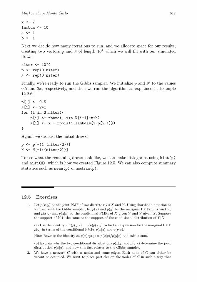
Markov chain Monte Carlo 517
x <- 7
lambda <- 10
a <- 1
b <- 1
Next we decide how many iterations to run, and we allocate space for our results,creating two vectors p and N of length 104 which we will fill with our simulateddraws:
niter <- 10^4
p <- rep(0,niter)
N <- rep(0,niter)
Finally, we’re ready to run the Gibbs sampler. We initialize p and N to the values0.5 and 2x, respectively, and then we run the algorithm as explained in Example12.2.6:
p[1] <- 0.5
N[1] <- 2*x
for (i in 2:niter){
p[i] <- rbeta(1,x+a,N[i-1]-x+b)
N[i] <- x + rpois(1,lambda*(1-p[i-1]))
}
Again, we discard the initial draws:
p <- p[-(1:(niter/2))]
N <- N[-1:(niter/2))]
To see what the remaining draws look like, we can make histograms using hist(p)
and hist(N), which is how we created Figure 12.5. We can also compute summarystatistics such as mean(p) or median(p).
12.5 Exercises
1. Let p(x, y) be the joint PMF of two discrete r.v.s X and Y . Using shorthand notation aswe used with the Gibbs sampler, let p(x) and p(y) be the marginal PMFs of X and Y ,and p(x|y) and p(y|x) be the conditional PMFs of X given Y and Y given X. Supposethe support of Y is the same as the support of the conditional distribution of Y |X.
(a) Use the identity p(x)p(y|x) = p(y)p(x|y) to find an expression for the marginal PMFp(y) in terms of the conditional PMFs p(x|y) and p(y|x).
Hint: Rewrite the identity as p(x)/p(y) = p(x|y)/p(y|x) and take a sum.
(b) Explain why the two conditional distributions p(x|y) and p(y|x) determine the jointdistribution p(x|y), and how this fact relates to the Gibbs sampler.
2. We have a network G with n nodes and some edges. Each node of G can either bevacant or occupied. We want to place particles on the nodes of G in such a way that

518 Introduction to Probability
the particles are not too crowded. Thus, define a feasible configuration as a placementof particles such that each node is occupied by at most one particle, and no neighbor ofan occupied node is occupied.
Construct a Markov chain whose stationary distribution is uniform over all feasibleconfigurations. Clearly specify the transition rule of your Markov chain, and explainwhy its stationary distribution is uniform.
3. This problem considers an application of MCMC techniques to image analysis. Imaginea 2D image consisting of an L⇥L grid of black-or-white pixels. Let Yj be the indicatorof the jth pixel being white, for j = 1, . . . , L2. Viewing the pixels as nodes in a network,the neighbors of a pixel are the pixels immediately above, below, to the left, and to theright (except for boundary cases).
Let i ⇠ j stand for “i and j are neighbors”. A commonly used model for the joint PMFof Y = (Y
1
, . . . , YL2
) is
P (Y = y) / exp
0
@�X
(i,j):i⇠j
I(yi = yj)
1
A .
If � is positive, this says that neighboring pixels prefer to have the same color. The
normalizing constant of this joint PMF is a sum over all 2L2
possible configurations, soit may be very computationally di�cult to obtain. This motivates the use of MCMC tosimulate from the model.
(a) Suppose that we wish to simulate random draws from the joint PMF of Y, for aparticular known value of �. Explain how we can do this using Gibbs sampling, cyclingthrough the pixels one by one in a fixed order.
(b) Now provide a Metropolis-Hastings algorithm for this problem, based on a proposalof picking a uniformly random site and toggling its value.

13
Poisson processes
Poisson processes serve as a simple model for events occurring in time or space: inone dimension, cars passing by a highway checkpoint; in two dimensions, flowers ina meadow; in three dimensions, stars in a region of the galaxy. Poisson processes area primary building block for more complicated processes in time and space, whichare the focus of a branch of statistics called spatial statistics.
Poisson processes are also useful in probability, as they tie together many of thenamed distributions and provide us with insightful story proofs for results thatmight otherwise be tedious to show. This leads to a new problem-solving strategy,which we will demonstrate: even when a problem makes no mention of Poissonprocesses, there are sometimes ways to pretend the r.v.s are coming from a Poissonprocess so that we can use convenient Poisson process properties.
In this chapter, we’ll review the already familiar definition of the 1D Poisson process,derive and discuss three important properties of the 1D Poisson process, and thenextend these properties to Poisson processes in higher dimensions.
13.1 Poisson processes in one dimension
In Section 5.6, we defined a one-dimensional Poisson process and showed that theinterarrival times are i.i.d. Exponentials. In Chapter 8 we showed that the time ofthe jth arrival (relative to some fixed starting time) is Gamma. Let’s review theseresults, with notation that will help us generalize to higher dimensions.
Definition 13.1.1 (1D Poisson process). A sequence of arrivals in continuous timeis a Poisson process with rate � if
1. the number of arrivals in an interval of length t is distributed Pois(�t);
2. the numbers of arrivals in disjoint time intervals are independent.
Usually we will assume that the timeline starts at t = 0, in which case we have aPoisson process on (0,1), but we can use the same conditions to define a Poissonprocess on (�1,1) if we want the timeline to be infinite in both directions.
519

520 Introduction to Probability
Consider a Poisson process on (0,1). Departing slightly from our notation in pre-vious chapters, let N(t) be the number of arrivals in (0, t]. Then the number ofarrivals in (t
1
, t2
] is N(t2
) � N(t1
), for 0 < t1
< t2
. Let Tj be the time of the jtharrival. Since T
1
> t is the same event as N(t) = 0 (this is the count-time duality,as discussed in Section 5.6), we have
P (T1
> t) = P (N(t) = 0) = e��t,
so T1
⇠ Expo(�). Next let’s condition on the first arrival time T1
and look at theadditional time T
2
� T1
until the second arrival. We have T2
� T1
|T1
⇠ Expo(�) bythe same argument as above, since we have a fresh Poisson process starting at T
1
.Since the conditional distribution of T
2
�T1
|T1
does not depend on T1
, we have thatT2
� T1
is independent of T1
, and so T2
� T1
⇠ Expo(�) unconditionally too.
Continuing in this way, all the interarrival times Tj � Tj�1
are i.i.d. Expo(�) r.v.s.So a Poisson process can be described dually as a process in which arrival countsare Poissons, or a process in which interarrival times are Exponentials. Since Tj isthe sum of j i.i.d. Expo(�) r.v.s, we have Tj ⇠ Gamma(j,�).
This connection with the Exponential tells us how we can generate n arrivals froma Poisson process.
Story 13.1.2 (Generative story for 1D Poisson process). To generate n arrivalsfrom a Poisson process on (0,1) with rate �:
1. Generate n i.i.d. Expo(�) r.v.s X1
, . . . , Xn.
2. For j = 1, . . . , n, set Tj = X1
+ · · ·+Xj .
Then we can take T1
, . . . , Tn to be the arrival times. ⇤
0 10
λ = 1
λ = 2
λ = 5
FIGURE 13.1
Simulated Poisson process in one dimension, for � = 1, 2, 5.
Figure 13.1 depicts three realizations of Poisson processes with rates 1, 2, and 5,respectively, plotted up to time 10. In all three cases, we can see that despite the in-terarrival times being i.i.d., the arrivals are not evenly spaced. Rather, there is a lot

Poisson processes 521
of variability in the interarrival times, which produces clumps of arrivals. This phe-nomenon is known as Poisson clumping. It might seem like an amazing coincidenceto observe a cluster of several arrivals that are close together in time, but Poissonclumping says that having such clusters is common with Poisson processes.
13.2 Conditioning, superposition, thinning
The three most important properties to understand about the Poisson process areconditioning, superposition, and thinning. These correspond to properties we’ve al-ready seen about the Poisson distribution, so they should already be plausible.
13.2.1 Conditioning
What happens when we take a Poisson process and condition on the total numberof events in an interval? Our first result is that conditional on the total number ofevents in an interval, the number of events in a fixed subinterval is Binomial. Thisfollows from Theorem 4.8.2, where we showed that we can get from the Poisson tothe Binomial by conditioning.
Theorem 13.2.1 (Conditional counts). Let {N(t), t > 0} be a Poisson process withrate �, and let t
1
< t2
. Then the conditional distribution of N(t1
) given N(t2
) = nis
N(t1
) | N(t2
) = n ⇠ Bin
✓n,
t1
t2
◆.
0 t1 t2
N(t1) N(t2) - N(t1)
FIGURE 13.2
Conditioning. Given that n arrivals occurred in (0, t2
], the conditional distributionof the number of arrivals in (0, t
1
] is Binomial with parameters n and t1
/t2
.
Proof. Figure 13.2 illustrates the setup. The claim is that conditional on having ntotal arrivals in (0, t
2
], each arrival becomes an independent Bernoulli trial, landingto the left of t
1
with probability t1
/t2
; thus N(t1
) is Binomial.
For the proof, we use the independence of disjoint intervals. Since the intervals(0, t
1
] and (t1
, t2
] are disjoint, N(t1
) is independent of N(t2
) � N(t1
). The first is
522 Introduction to Probability
distributed Pois(�t1
), the second is distributed Pois(�(t2
� t1
)), and their sum isthe total number of arrivals in (0, t
2
], namely N(t2
). By Theorem 4.8.2,
N(t1
) | N(t2
) = n ⇠ Bin
✓n,
�t1
�t1
+ �(t2
� t1
)
◆,
which is precisely what we want to show. ⌅
Our proof would hold equally well for any subinterval of length t1
. This tells us thatthe probability of an arrival falling into a subinterval of length t
1
is proportionalto t
1
, regardless of where the subinterval is located. Carrying this one step further,for all x < t
2
, the probability of an arrival falling into a subinterval of lengthx is proportional to x. But probability proportional to length is the story of theUniform distribution! Therefore, conditional on N(t
2
) = n, it is as though we placedn arrivals uniformly at random on the interval (0, t
2
]. The jth arrival time is simplythe jth order statistic of these randomly placed arrivals.
Theorem 13.2.2 (Conditional times). In a Poisson process of rate �, conditionalon N(t) = n, the arrival times T
1
, . . . , Tn are distributed as the order statistics of ni.i.d. Unif(0, t) r.v.s.
From Chapter 8, we know that the order statistics of Unif(0, 1) r.v.s are Betas, sothe conditional distribution of the Tj are scaled Betas; to get Beta distributions, wecan just divide the Tj by t so that their support is between 0 and 1:
t�1Tj | N(t) = n ⇠ Beta(j, n� j + 1).
We now have another way to generate arrivals from a Poisson process, this time fora specific interval instead of a specific number of arrivals.
Story 13.2.3 (Generative story for Poisson process, take 2). To generate arrivalsfrom a Poisson process with rate � in an interval (0, t]:
1. Generate the total number of events in the interval, N(t) ⇠ Pois(�t).
2. Given N(t) = n, generate n i.i.d. Unif(0, t) r.v.s U1
, . . . , Un.
3. For j = 1, . . . , n, set Tj = U(j).
⇤This is actually the generative story we used to create Figure 13.1, since we knewwe wanted to simulate in the interval (0, 10].
Example 13.2.4 (Users on a website). Users visit a certain website according toa Poisson process with rate �
1
users per minute, where an “arrival” at a certaintime means that at that time someone starts browsing the site. After arriving at thesite, each user browses the site for an Expo(�
2
) amount of time (and then leaves),independently of other users.

Poisson processes 523
Suppose that at time 0, no one is using the site. Let Nt be the number of userswho arrive in the interval (0, t], and let Ct be the number of users who are currentlybrowsing the site at time t.
(a) Let X be the time of arrival and Y be the time of departure for a user whoarrives at a Uniform time point in [0, t] (viewed as points on the timeline). Find thejoint PDF of X and Y .
(b) Let pt be the probability that a user who arrives at a Uniform time point in(0, t] is still browsing the site at time t. Find pt.
(c) Find the distribution of Ct in terms of �1
,�2
, and t.
(d) Little’s law is a very general result, which says the following:
The long-run average number of customers in a stable system is the long-term av-erage arrival rate multiplied by the average time a customer spends in the system.
Explain what happens to E(Ct) for t large, and how this can be interpreted in termsof Little’s law.
Solution:
(a) We have X ⇠ Unif(0, t). Given X = x, Y is an Expo(�2
) shifted to start at x,i.e., (Y � x)|(X = x) ⇠ Expo(�
2
). So the joint PDF of X and Y is
f(x, y) = fX(x)fY |X(y|x) = �2
te��
2
(y�x),
for 0 < x < t and x < y.
(b) With notation as in (a), we want to find pt = P (Y > t). This can be done byintegrating the joint PDF over all (x, y) with y > t:
P (Y > t) =1
t
Z t
0
Z 1
t�2
e��2
(y�x)dydx
=1
t
Z t
0
e�2
x
✓Z 1
t�2
e��2
ydy
◆dx
=e��
2
t
t
Z t
0
e�2
xdx
=e��
2
t
�2
t
⇣e�2
t � 1⌘
=1� e��
2
t
�2
t.
Alternatively, we can view Y as a convolution of a Unif(0, 1) r.v. and an Expo(�2
)r.v., and use facts about convolutions to get the distribution of Y .
(c) By Theorem 13.2.2, given Nt = n we have that the n arrival times in (0, t] are

524 Introduction to Probability
i.i.d. and uniform in that interval. Therefore, Ct|Nt ⇠ Bin(Nt, pt), with pt as above,and Nt ⇠ Pois(�
1
t). So by the chicken-egg story (Example 7.1.9),
Ct ⇠ Pois(�1
ptt).
That is,
Ct ⇠ Pois
✓�1
(1� e��2
t)
�2
◆.
(d) As t ! 1, E(Ct) ! �1
/�2
. This agrees exactly with Little’s law since it saysthat the long-run average number of users “in the system” (currently browsing thesite) is the rate at which users arrive (�
1
) times the average time a user browses ina session (1/�
2
). ⇤
13.2.2 Superposition
The second property of Poisson processes is superposition: if we take two inde-pendent Poisson processes and overlay them, we get another Poisson process. Thisfollows from the fact that the sum of independent Poissons is Poisson.
Theorem 13.2.5 (Superposition). Let {N1
(t), t > 0} and {N2
(t), t > 0} be inde-pendent Poisson processes with rates �
1
and �2
, respectively. Then the combinedprocess N(t) = N
1
(t) +N2
(t) is a Poisson process with rate �1
+ �2
.
Proof. Let’s verify the two properties in the definition of Poisson process.
1. For all t > 0, N1
(t) ⇠ Pois(�1
t) and N2
(t) ⇠ Pois(�2
t), independently, so N(t) ⇠Pois((�
1
+ �2
)t) by Theorem 4.8.1. The same argument applies for any interval oflength t, not just intervals of the form (0, t].
2. Arrivals in disjoint intervals are independent in the combined process becausethey are independent in the two individual processes, and the individual processesare independent of each other. ⌅
In particular, the interarrival times in the combined Poisson process arei.i.d. Expo(�
1
+ �2
).
The most transparent way to generate from the superposition of two Poisson pro-cesses is exactly as one would expect: generate from the individual Poisson processes,then superpose them.
Story 13.2.6 (Generative story for superposed Poisson process). To generate fromthe superposition of two Poisson processes with rates �
1
and �2
in the interval [0, t):
1. Generate arrivals from the Poisson process with rate �1
using Story13.2.3.

Poisson processes 525
2. Generate arrivals from the Poisson process with rate �2
using Story13.2.3.
3. Superpose the results of steps 1 and 2.
⇤
0 10
λ1 = 0.5
λ2 = 0.5
λ1 + λ2 = 1
FIGURE 13.3
Superposition. The superposition of independent Poisson processes is a Poissonprocess, and the rates add. The top two timelines are independent Poisson processes,each with rate 0.5. The bottom timeline is the superposition of the top two Poissonprocesses and is itself a Poisson process with rate 1.
Figure 13.3 depicts a superposed Poisson process consisting of ⇥’s and ⇧’s. Let’scall the ⇥’s “type-1 events” and the ⇧’s “type-2 events”. A natural question to askis: what is the probability of observing a type-1 event before a type-2 event?
Theorem 13.2.7 (Probability of type-1 event before type-2 event). If independentPoisson processes of rates �
1
and �2
are superposed, the probability of a type-1event before a type-2 event in the combined Poisson process is �
1
/(�1
+ �2
).
Proof. Let T be the time until the first type-1 event and let V be the time until thefirst type-2 event. We seek P (T V ). We could do this with 2D LOTUS, integratingthe joint PDF of T and V over the region of interest in the 2D plane. But it turnsout we can avoid calculus altogether. We know T ⇠ Expo(�
1
) and V ⇠ Expo(�2
),so by applying scale transformations, T = �
1
T and V = �2
V are i.i.d. Expo(1).Letting U = T /(T + V ), we have
P (T V ) = P
T
�1
V
�2
!
= P
T
T + V V
T + V· �1�2
!
= P
✓U (1� U) · �1
�2
◆
= P
✓U �
1
�1
+ �2
◆.

526 Introduction to Probability
Since T and V are both Expo(1) or Gamma(1, 1), the bank–post o�ce story tellsus that U ⇠ Beta(1, 1). In other words, U is standard Uniform! (One might haveguessed this from our choice of notation.) Therefore
P (T V ) = P
✓U �
1
�1
+ �2
◆=
�1
�1
+ �2
.
When �1
= �2
, this reduces to 1/2, as it should by symmetry. ⌅
The above result applies to the first arrival in the combined Poisson process. Afterthe first arrival, however, the same reasoning applies to the second arrival: by thememoryless property, the time to the next type-1 event is Expo(�
1
) and the timeto the next type-2 event is Expo(�
2
), independent of the past. Therefore the secondarrival is a type-1 arrival with probability �
1
/(�1
+ �2
), independent of the firstarrival. Similarly, all of the arrival types can be viewed as i.i.d. coin tosses withprobability �
1
/(�1
+ �2
) of landing Heads.
This yields an alternative generative story for the superposition of two Poissonprocesses: we can first generate an Expo(�
1
+ �2
) r.v. to decide when the nextarrival occurs, and then independently flip a coin with probability �
1
/(�1
+ �2
) ofHeads to decide what kind of arrival it is.
Story 13.2.8 (Generative story for superposed Poisson process, take 2). To gen-erate n arrivals from the superposition of two Poisson processes with rates �
1
and�2
:
1. Generate n i.i.d. Expo(�1
+ �2
) r.v.s X1
, . . . , Xn, and set T(j) = X
1
+· · ·+Xj .
2. Generate n Bern(�1
/(�1
+ �2
)) r.v.s I1
, . . . , In, which are independentof each other and of the Xj . Let the jth arrival be type-1 if Ij = 1 andtype-2 otherwise.
⇤This story provides us with a quick proof of a result known as the competing riskstheorem, which seems like a surprising independence result when stated on its ownbut becomes very intuitive when viewed in the context of Poisson processes.
Example 13.2.9 (Competing risks). The lifetime of Fred’s refrigerator is Y1
⇠Expo(�
1
), and the lifetime of Fred’s dishwasher is Y2
⇠ Expo(�2
), independent ofY1
. Show that min(Y1
, Y2
), the time of the first appliance failure, is independent ofI(Y
1
< Y2
), the indicator that the refrigerator failed first.
Solution:
Here we encounter our first instance of the embedding strategy : this problem doesn’tmention Poisson processes anywhere, but we will embed the r.v.s Y
1
and Y2
into aPoisson process that we ourselves invent, in order to take advantage of the properties

Poisson processes 527
of Poisson processes. So let’s pretend there is an entire Poisson process of refrigeratorfailures with rate �
1
and a Poisson process of dishwasher failures with rate �2
. Thenwe can interpret Y
1
as the waiting time for the first arrival in the refrigerator processand Y
2
as the waiting time for the first arrival in the dishwasher process.
Furthermore, min(Y1
, Y2
) is the waiting time for the first arrival in the superpositionof the two Poisson processes, and I(Y
1
< Y2
) is the indicator of this arrival being atype-1 event. But as we know from the above generative story, the waiting times andevent types in a superposed Poisson process are generated completely independently!Therefore min(Y
1
, Y2
) and I(Y1
< Y2
) are independent. This says that knowing therefrigerator was the first appliance to fail does not provide any information aboutthe time of the first appliance failure. ⇤
A direct consequence of the generative story is that if we project a superposedPoisson process into discrete time, keeping the sequence of type-1 and type-2 arrivalsbut not the arrival times themselves, we are left with i.i.d. Bern(�
1
/(�1
+ �2
))r.v.s I
1
, I2
, . . . , where Ij is the indicator of the jth arrival being type-1. Figure13.4 illustrates what it means to remove the continuous-time information from thePoisson process, and Theorem 13.2.10 states the result formally.
...
FIGURE 13.4
Projection into discrete time. Stripping out the continuous-time information from asuperposed Poisson process produces a sequence of i.i.d. indicators of type-1 versustype-2 events. Here ⇥ represents type-1 events and ⇧ represents type-2 events.
Theorem 13.2.10 (Projection of superposition into discrete time). Let {N(t), t >0} be the superposition of two independent Poisson processes with rates �
1
and �2
.For j = 1, 2, . . . , let Ij be the indicator of the jth event being from the Poissonprocess with rate �
1
. Then the Ij are i.i.d. Bern(�1
/(�1
+ �2
)).
Using this result, we can prove with a story that a Gamma mixture of Poissons isNegative Binomial, which we learned from Fred in Blotchville (Story 8.4.5). In thatexample we found the marginal distribution by integration, but now we can do itwithout any manipulation of PDFs. We’ll consider a special case first.
Theorem 13.2.11 (Exponential mixture of Poissons is Geometric). Let X ⇠Expo(�) and Y |X = x ⇠ Pois(x). Then Y ⇠ Geom(�/(�+ 1)).
Proof. As with the competing risks theorem, we embed X and Y into Poissonprocesses. Consider two independent Poisson processes, a process of failures arrivingat rate 1 and another of successes arriving at rate �. Let X be the time of the first

528 Introduction to Probability
success; then X ⇠ Expo(�). Let Y be the number of failures before the time of thefirst success. By the definition of a Poisson process with rate 1, Y |X = x ⇠ Pois(x).Therefore X and Y satisfy the conditions of the theorem.
To get the marginal distribution of Y , strip out the continuous-time information!In discrete time we have i.i.d. Bernoulli trials with success probability �/(� + 1),and Y is defined as the number of failures before the first success, so by the storyof the Geometric distribution, Y ⇠ Geom(�/(�+ 1)). ⌅
The reasoning for the general case is analogous.
Theorem 13.2.12 (Gamma mixture of Poissons is Negative Binomial). Let X ⇠Gamma(r,�) and Y |X = x ⇠ Pois(x). Then Y ⇠ NBin(r,�/(�+ 1)).
Proof. Consider two independent Poisson processes, a process of failures arrivingat rate 1 and another of successes arriving at rate �. Let X be the time of the rthsuccess, so X ⇠ Gamma(r,�). Let Y be the number of failures before the time of therth success. Then Y |X = x ⇠ Pois(x) by the definition of Poisson process. We havethat Y is the number of failures before the rth success in a sequence of i.i.d. Bernoullitrials with success probability �/(�+ 1), so Y ⇠ NBin(r,�/(�+ 1)). ⌅
13.2.3 Thinning
The third property of Poisson processes is thinning : if we take a Poisson processand, for each arrival, independently flip a coin to decide whether it is a type-1event or type-2 event, we end up with two independent Poisson processes. This isthe converse of superposition, and it follows from the chicken-egg story, which weintroduced in Chapter 7.
Theorem 13.2.13 (Thinning). Let {N(t), t > 0} be a Poisson process with rate�, and classify each arrival in the process as a type-1 event with probability p anda type-2 event with probability 1 � p, independently. Then the type-1 events forma Poisson process with rate �p, the type-2 events form a Poisson process with rate�(1� p), and these two processes are independent.
Proof. Let’s verify that the type-1 process, which we’ll denote by {N1
(t), t > 0},satisfies the two properties in the definition of Poisson process.
1. Let’s show that the number of arrivals for the type-1 process in an interval oflength t is distributed Pois(�pt). For all t > 0, N(t) ⇠ Pois(�t) by definition, andN
1
(t)|N(t) = n ⇠ Bin(n, p) by the story of the Binomial distribution. Then by thechicken-egg story (Example 7.1.9), N
1
(t) ⇠ Pois(�pt). The same reasoning appliesfor any interval of length t, not just intervals of the form (0, t].
2. Arrivals in disjoint intervals are independent in the type-1 process because theyare a subset of the arrivals in the full process, and we know the full process satisfiesindependence of disjoint intervals.

Poisson processes 529
Therefore, {N1
(t), t > 0} is a Poisson process with rate �p. The same reasoningapplies for showing that the type-2 process, {N
2
(t), t > 0}, is a Poisson processwith rate �(1� p). The two processes are independent because for all t > 0, N
2
(t)is independent of N
1
(t) by the chicken-egg story. ⌅
Thus we can superpose independent Poisson processes to get a combined Poissonprocess, or we can split a single Poisson process into independent Poisson processes.Figure 13.5 is an illustration of thinning. We simply flipped Figure 13.3 upside-down,but this is appropriate because thinning is the flip side of superposition!
λp = 0.5
λ(1 - p) = 0.5
λ = 1
0 10
FIGURE 13.5
Thinning. Starting with a single Poisson process, if we let each arrival be type-1with probability p and type-2 with probability 1 � p, we obtain two independentPoisson processes with rates �p and �(1� p). Here ⇥ represents type-1 events and⇧ represents type-2 events, and we take p = 0.5.
Example 13.2.14 (First Success sum of Exponentials). Let X1
, X2
, . . . bei.i.d. Expo(�), and let N ⇠ FS(p), independent of the Xj . What is the distribution
of Y =PN
j=1
Xj?
Solution:
We’ll solve this problem twice, first with tools from Chapter 9 and then with aPoisson process story that uses thinning. For the first method, we recognize Y asthe sum of a random number of random variables, so we can find the MGF of Yusing Adam’s Law, conditioning on N . Recalling that the MGF of the Expo(�)distribution is �/(�� t) for t < �, we have
E�etY�= E
⇣E⇣et
PN
j=1
Xj
��N⌘⌘
= E�E�etX1
�E�etX2
�. . . E
�etXN
�|N�
= E⇣E�etX1
�N⌘
= E
✓�
�� t
◆N!.

530 Introduction to Probability
Now we can use LOTUS with the FS(p) PMF,
P (N = k) = qk�1p for k = 1, 2, . . .
The LOTUS sum is
E
✓�
�� t
◆N!
=1X
k=1
✓�
�� t
◆k
qk�1p,
which simplifies to �p/(�p � t) after a bit of algebra. This is the Expo(�p) MGF,so Y ⇠ Expo(�p).
Now let’s see how Poisson processes can spare us from algebra while also providinginsight into why Y is Exponential. Using the embedding strategy, since the Xj
are i.i.d. Expo(�), we are free to interpret the Xj as interarrival times in a Poissonprocess with rate �. So let’s imagine such a Poisson process, and let’s further imaginethat each of the arrivals is a special arrival with probability p, independently. Thenwe can interpret N as the number of arrivals until the first special arrival and Yas the waiting time for the first special arrival. But by the thinning property, thespecial arrivals form a Poisson process with rate �p. The waiting time for the firstspecial arrival is thus distributed Expo(�p). ⇤The next example shows how thinning can help us decompose a complicated Poissonprocess into more manageable components.
Example 13.2.15 (Cars on a highway). Suppose cars enter a one-way highwayfrom a common entrance, following a Poisson process with rate �. The ith car hasvelocity Vi and travels at this velocity forever; no time is lost when one car overtakesanother car. Assume the Vi are i.i.d. discrete r.v.s whose support is a finite set ofpositive values. The process starts at time 0, and we’ll consider the highway entranceto be at location 0.
For fixed locations a and b on the highway with 0 < a < b, let Zt be the number ofcars located in the interval [a, b] at time t. (For instance, on an interstate highwayrunning west to east through the midwestern United States, a could be KansasCity and b could be St. Louis; then Zt would be the number of cars on the highwaythat are in the state of Missouri at time t.) Figure 13.6 illustrates the setup of theproblem and the definition of Zt.
Assume t is large enough that t > b/Vi for all possible values of Vi. Show that Zt
has a Poisson distribution with mean �(b� a)E(V �1
i ).
Solution:
Since the Vi are discrete with finite support, we can enumerate the set of possiblevelocities v
1
, . . . , vm and their probabilities p1
, . . . , pm. After doing so, we realize thatthe cars entering the highway represent m types of arrivals, each corresponding to adi↵erent velocity. This suggests breaking up our overall Poisson process into simplerones. Let’s thin the Poisson process m ways according to the velocity of the cars,

Poisson processes 531
0+ + +++ ++ +
timet
dista
nce a
long
high
way
a
b
0
FIGURE 13.6
Cars enter a highway. Their entrance times form a Poisson process and are indicatedby ⇥’s on the time axis. The ith car has velocity Vi, represented by the slope ofthe line emanating from the ith ⇥ symbol. We are interested in Zt, the number ofcars located in the interval [a, b] at time t. Here we observe Zt = 3, depicted by thethree stars.
resulting in a Poisson process with rate �p1
for cars of velocity v1
, a Poisson processwith rate �p
2
for cars of velocity v2
, and so forth.
For each of these thinned Poisson processes, we can ask: within what time intervaldo cars from this process have to enter the highway in order to be in [a, b] at timet? This is a matter of physics, not statistics:
distance = velocity · time,
so a car that enters the highway at time s with velocity v will be at position (t�s)vat time t. Thus, in order for the car’s position to be between a and b, we requireits arrival time to be between t � b/v and t � a/v. (By our assumption that t issu�ciently large, we don’t need to worry about t � b/v being negative.) If the cararrives prior to time t�b/v, it will already have passed b by time t; if the car arrivesafter time t� a/v, it won’t have reached a by time t.
We now have the answer for each thinned Poisson process considered on its own.Within the process where cars have velocity vj , the number of cars arriving betweent�b/vj and t�a/vj , which we’ll call Ztj , is distributed Pois(�pj(b�a)/vj): the rate ofthe process is �pj , and the length of the interval [t�b/vj , t�a/vj ] is (b�a)/vj . Sincethe thinned processes are independent, Zt1 through Ztm are independent Poissonr.v.s. Thus
Zt = Zt1 + · · ·+ Ztm ⇠ Pois
0
@�(b� a)mX
j=1
pjvj
1
A ,
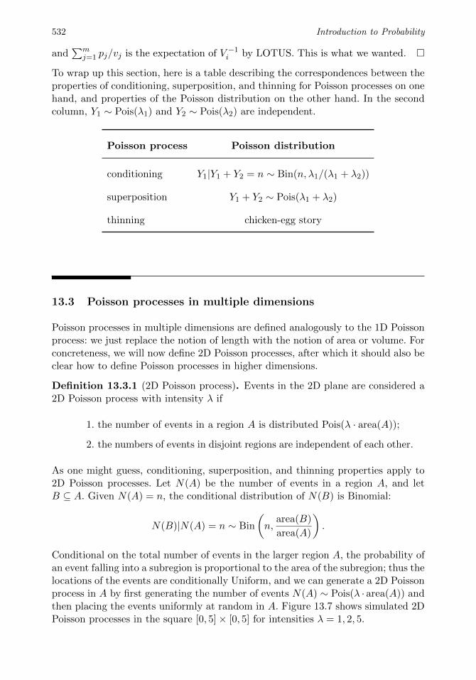
532 Introduction to Probability
andPm
j=1
pj/vj is the expectation of V �1
i by LOTUS. This is what we wanted. ⇤
To wrap up this section, here is a table describing the correspondences between theproperties of conditioning, superposition, and thinning for Poisson processes on onehand, and properties of the Poisson distribution on the other hand. In the secondcolumn, Y
1
⇠ Pois(�1
) and Y2
⇠ Pois(�2
) are independent.
Poisson process Poisson distribution
conditioning Y1
|Y1
+ Y2
= n ⇠ Bin(n,�1
/(�1
+ �2
))
superposition Y1
+ Y2
⇠ Pois(�1
+ �2
)
thinning chicken-egg story
13.3 Poisson processes in multiple dimensions
Poisson processes in multiple dimensions are defined analogously to the 1D Poissonprocess: we just replace the notion of length with the notion of area or volume. Forconcreteness, we will now define 2D Poisson processes, after which it should also beclear how to define Poisson processes in higher dimensions.
Definition 13.3.1 (2D Poisson process). Events in the 2D plane are considered a2D Poisson process with intensity � if
1. the number of events in a region A is distributed Pois(� · area(A));
2. the numbers of events in disjoint regions are independent of each other.
As one might guess, conditioning, superposition, and thinning properties apply to2D Poisson processes. Let N(A) be the number of events in a region A, and letB ✓ A. Given N(A) = n, the conditional distribution of N(B) is Binomial:
N(B)|N(A) = n ⇠ Bin
✓n,
area(B)
area(A)
◆.
Conditional on the total number of events in the larger region A, the probability ofan event falling into a subregion is proportional to the area of the subregion; thus thelocations of the events are conditionally Uniform, and we can generate a 2D Poissonprocess in A by first generating the number of events N(A) ⇠ Pois(� · area(A)) andthen placing the events uniformly at random in A. Figure 13.7 shows simulated 2DPoisson processes in the square [0, 5]⇥ [0, 5] for intensities � = 1, 2, 5.

Poisson processes 533
FIGURE 13.7
Simulated 2D Poisson process in the square [0, 5]⇥ [0, 5], for � = 1, 2, 5.
As in the 1D case, the superposition of independent 2D Poisson processes is a 2DPoisson process, and the intensities add. We can also thin a 2D Poisson process toget independent 2D Poisson processes.
The only property of 1D Poisson processes for which we haven’t asserted a higher-dimensional analog is count-time duality. The next example, the last in this chapter,will lead us to a count-distance duality.
Example 13.3.2 (Nearest star). Stars in a certain universe are distributed accord-ing to a 3D Poisson process with intensity �. If you live in this universe, what isthe distribution of the distance from you to the nearest star?
Solution:
In a 3D Poisson process with intensity �, the number of events in a region of spaceV is Poisson with mean � · volume(V ). Let R be the distance from you to thenearest star. The key observation is that in order for the event R > r to occur,there must be no stars within a sphere of radius r around you; in fact, these twoevents are equivalent. Let Nr be the number of events within radius r of you, soNr ⇠ Pois(� · 4
3
⇡r3). Then
R > r is the same event as Nr = 0,
soP (R > r) = P (Nr = 0) = e�
4
3
�⇡r3 .
This specifies the CDF and hence the distribution of R. The distribution of R is anexample of a Weibull distribution, which generalizes the Exponential. ⇤Poisson processes have numerous generalizations, some of which are explored in theexercises. We can allow � to vary as a function of time or space instead of remainingconstant; a Poisson process with varying � is called inhomogeneous. We can alsoallow � to be a random variable; this is called a Cox process. Finally, we can allow� to grow with each successive arrival; this is called a Yule process.

534 Introduction to Probability
13.4 Recap
A Poisson process in one dimension is a sequence of arrivals such that the numberof arrivals in any interval is Poisson and disjoint intervals are independent. Someoperations that we can perform with Poisson processes are conditioning, superposi-tion, and thinning. Conditioning on the total number of arrivals in an interval allowsus to view the arrivals as independent Uniforms on the interval. Superposition andthinning are complementary, and they allow us to split and merge Poisson processeswhen convenient. All of these properties have analogs for higher dimensions.
Poisson processes tie together many of the named distributions we have studied inthis book:
• Poisson for the arrival counts,
• Exponential and Gamma for the interarrival times and arrival times,
• Binomial for the conditional counts,
• Uniform and (scaled) Beta for the conditional arrival times,
• Geometric and Negative Binomial for the discrete waiting times for special arrivals.
Poisson processes are also especially amenable to story proofs. A problem-solvingstrategy we used several times in this chapter is to embed r.v.s into a Poisson processin the hopes of discovering a story proof, even when the original problem appearsto be unrelated to Poisson processes.
Poisson processes unite two of the important themes of this book, named distribu-tions and stories, in a natural way. We think it is fitting to end with a topic thatweaves together the story threads from throughout the book.
13.5 R
1D Poisson process
In Chapter 5, we discussed how to simulate a specified number of arrivals from aone-dimensional Poisson process by using the fact that the interarrival times arei.i.d. Exponentials. In this chapter, Story 13.2.3 tells us how to simulate a Poissonprocess within a specified interval (0, L]. We first generate the number of arrivalsN(L), which is distributed Pois(�L). Conditional on N(L) = n, the arrival timesare distributed as the order statistics of n i.i.d. Unif(0, L) r.v.s. The following codesimulates arrivals from a Poisson process with rate 10 in the interval (0, 5]:

Poisson processes 535
L <- 5
lambda <- 10
n <- rpois(1,lambda*L)
t <- sort(runif(n,0,L))
To visualize the Poisson process we have generated, we can plot the cumulativenumber of arrivals N(t) as a function of t:
plot(t,1:n,type="s")
This produces a staircase plot as in Figure 13.8.
0 1 2 3 4 5
010
2030
4050
t
N(t)
FIGURE 13.8
Number of arrivals in a Poisson process with rate 10 in the interval (0, 5].
Thinning
The following code starts with a vector of arrival times t and the correspondingnumber of arrivals n, generated according to the previous section. For each arrival,we flip a coin with probability p of Heads; these coin tosses are stored in the vectory. Finally, the arrivals for which the coin landed Heads are labeled as type-1; the restare labeled as type-2. The resulting vectors of arrival times t
1
and t2
are realizationsof independent Poisson processes, by Theorem 13.2.13. To perform this in R withp = 0.3, we can type
p <- 0.3
y <- rbinom(n,1,p)
t1 <- t[y==1]
t2 <- t[y==0]
As before, we can plot the number of arrivals in each Poisson process, N1
(t) andN
2
(t), as a function of t.

536 Introduction to Probability
0 1 2 3 4 5
12
34
56
7
t
N_1(t)
0 1 2 3 4 5
010
2030
40
t
N_2(t)
FIGURE 13.9
Number of arrivals in each of two independent Poisson processes with rates 3 and7 in the interval (0, 5].
2D Poisson process
Simulating a 2D Poisson process is nearly as straightforward as simulating a 1DPoisson process. In the square (0, L] ⇥ (0, L], the number of arrivals is distributedPois(�L2). Conditional on the number of arrivals, the locations of the arrivals areUniform over the square, so by Example 7.1.22, their horizontal and vertical coor-dinates can be generated independently:
L <- 5
lambda <- 10
n <- rpois(1,lambda*L^2)
x <- runif(n,0,L)
y <- runif(n,0,L)
We can then easily plot the locations of the arrivals as in Figure 13.7:
plot(x,y,pch=4)
13.6 Exercises
1. Passengers arrive at a bus stop according to a Poisson process with rate �. The arrivalsof buses are exactly t minutes apart. Show that on average, the sum of the waiting timesof the riders on one of the buses is 1
2
�t2.
2. Earthquakes occur over time according to a Poisson process with rate �. The jth earth-quake has intensity Zj , where the Zj are i.i.d. with mean µ and variance �2. Find themean and variance of the cumulative intensity of all the earthquakes up to time t.

Poisson processes 537
3. Alice receives phone calls according to a Poisson process with rate �. Unfortunately shehas lost her cell phone charger. The battery’s remaining life is a random variable T withmean µ and variance �2. Let N(T ) be the number of phone calls she receives before thebattery dies; find E(N(T )), Var(N(T )), and Cov(T,N(T )).
4. Emails arrive in Bob’s inbox according to a Poisson process with rate �, measuredin emails per hour; each email is work-related with probability p and personal withprobability 1 � p. The amount of time it takes to answer a work-related email is arandom variable with mean µW and variance �2
W , the amount of time it takes to answera personal email has mean µP and variance �2
P , and the response times for di↵erentemails are independent.
What is the average amount of time Bob has to spend answering all the emails thatarrive in a t-hour interval? What about the variance?
5. In an endless soccer match, goals are scored according to a Poisson process with rate �.Each goal is made by team A with probability p and team B with probability 1� p. Forj > 1, we say that the jth goal is a turnaround if it is made by a di↵erent team thanthe (j � 1)st goal; for example, in the sequence AABBA. . . , the 3rd and 5th goals areturnarounds.
(a) In n goals, what is the expected number of turnarounds?
(b) What is the expected time between turnarounds, in continuous time?
6. Let Nt be the number of arrivals up until time t in a Poisson process of rate �, and letTn be the time of the nth arrival. Consider statements of the form
P (Nt 71
n) = P (Tn 72
t) ,
where 71
and 72
are replaced by symbols from the list <,,�, >. Which of thesestatements are true?
7. Claims against an insurance company follow a Poisson process with rate � > 0. A totalof N claims were received over two periods of combined length t = t
1
+ t2
, with t1
andt2
being the lengths of the separate periods.
(a) Given this information, derive the (conditional) probability distribution of N1
, thenumber of claims made in the 1st period, given N .
(b) The amount paid for the ith claim is Xi, with X1
, X2
, . . . i.i.d. and independentof the claims process. Let E(Xi) = µ, Var(Xi) = �2, for i = 1, . . . , N . Given N , findthe mean and variance of the total claims paid in period 1. That is, find these twoconditional moments of the quantity
W1
=N
1X
i=1
Xi,
where (by convention) W1
= 0 if N1
= 0.
8. On a certain question-and-answer website, N ⇠ Pois(�1
) questions will be posted to-morrow, with �
1
measured in questions/day. Given N , the post times are i.i.d. anduniformly distributed over the day (a day begins and ends at midnight). When a ques-tion is posted, it takes an Expo(�
2
) amount of time (in days) for an answer to be posted,independently of what happens with other questions.
(a) Find the probability that a question posted at a uniformly random time tomorrowwill not yet have been answered by the end of that day.
(b) Find the joint distribution of how many answered and unanswered questions postedtomorrow there will be at the end of that day.
9. An inhomogeneous Poisson process in one dimension is a Poisson process whose rate,instead of being constant, is a nonnegative function �(t) of time. Formally, we require
538 Introduction to Probability
that the number of arrivals in the interval [t1
, t2
) be Poisson-distributed with meanR t2
t1
�(t)dt and that disjoint intervals be independent. When �(t) is constant, this reducesto the definition of the ordinary or homogeneous Poisson process.
(a) Show that we can generate arrivals from an inhomogeneous Poisson process in theinterval [t
1
, t2
) using the following procedure.
1. Let �max
be the maximum value of �(t) in the interval [t1
, t2
). Create a 2D rectangle[t1
, t2
)⇥ [0,�max
], and plot the function �(t) in the rectangle.
2. Generate N ⇠ Pois(�max
(t2
� t1
)), and place N points uniformly at random in therectangle.
3. For each of the N points: if the point falls below the curve �(t), accept it as anarrival in the process, and take its horizontal coordinate to be its arrival time. If thepoint falls above the curve �(t), reject it.
Hint: Verify that the two conditions in the definition are satisfied.
(b) Suppose we have an inhomogeneous Poisson process with rate function �(t). LetN(t)be the number of arrivals up to time t and Tj the time of the jth arrival. Explain whythe hybrid joint PDF of N(t) and T
1
, . . . , TN(t), which constitute all the data observedup to time t, is given by
f(n, t1
, . . . , tn) =e��
total�ntotal
n!· n!�(t1) . . .�(tn)
�ntotal
= e��total�(t
1
) . . .�(tn)
for 0 < t1
< t2
< · · · < tn and nonnegative integer n, where �total
=R t
0
�(u)du.
10. A Cox process is a generalization of a Poisson process, where the rate � is a randomvariable. That is, � is generated according to some distribution on (0,1) and then,given that value of �, a Poisson process with that rate is generated.
(a) Explain intuitively why disjoint intervals in a 1D Cox process are not independent.
(b) In a 1D Cox process where � ⇠ Gamma(↵,�), find the covariance between thenumber of arrivals in [0, t) and the number of arrivals in [t, t+ s).
Hint: Condition on �.
11. In a Yule process with rate �, the rate of arrivals increases after each new arrival, sothat the time between the (j � 1)st arrival and the jth arrival is distributed Expo(j�)for j = 1, 2, . . . . That is, interarrival times are independent but not i.i.d.
(a) Show that the superposition of two independent Yule processes with the same rateis a Yule process with rate 2�.
(b) Show that if we project the process from Part (a) into discrete time, the resultingsequence of type-1 and type-2 arrivals is equivalent to the following discrete-time process:
1. Start with two balls in an urn, labeled 1 and 2.
2. Draw a ball out of the urn at random, note its number, and replace it along withanother ball with the same number.
3. Repeat step 2 over and over.
12. Consider the coupon collector problem: n toy types, collected one by one, sampling withreplacement from the set of toy types each time. We solved this problem in Chapter 4,assuming that all toy types were equally likely to be collected. Now suppose that at eachstage, the jth toy type is collected with probability pj , where the pj are not necessarilyequal. Let N be the number of toys needed until we have a full set; we wish to findE(N). This problem outlines an embedding method for calculating E(N).
(a) Suppose that the toys arrive according to a Poisson process with rate 1, so that theinterarrival times between toys are i.i.d. Xj ⇠ Expo(1). For j = 1, . . . , n, let Yj be the

Poisson processes 539
waiting time until the first toy of type j. What are the distributions of the Yj? Are theYj independent?
(b) Explain why T = max(Y1
, . . . , Yn), the waiting time until all toy types are collected,can also be written as X
1
+ · · ·+XN , where the Xj are defined as in Part (a). Use thisto show that E(T ) = E(N).
(c) Show that E(T ), and hence E(N), can be found by computing the integral
Z 1
0
1�
nY
j=1
(1� e�pj
t)
!dt.
You can use the fact that E(T ) =R10
P (T > t)dt, which is explored in Exercise 20 fromChapter 5 and which also follows from writing
Z 1
0
P (T > t)dt =
Z 1
0
Z 1
t
f(u)dudt =
Z 1
0
f(u)
✓Z u
0
dt
◆du =
Z 1
0
uf(u)du,
where f is the PDF of T .


A
Math
A.1 Sets
A set is a Many that allows itself to be thought of as a One.– Georg Cantor
Amazon should put their cloud in a cloud, so the cloud will have the redundancyof the cloud.– @dowens
A set is a collection of objects. The objects can be anything: numbers, people,cats, courses, even other sets! The language of sets allows us to talk precisely aboutevents. If S is a set, then the notation x 2 S indicates that x is an element ormember of the set S (and x /2 S indicates that x is not in S). We can think of theset as a club, with precisely defined criteria for membership. For example:
1. {1, 3, 5, 7, . . . } is the set of all odd numbers;
2. {Worf, Jack, Tobey} is the set of Joe’s cats;
3. [3, 7] is the closed interval consisting of all real numbers between 3 and 7;
4. {HH,HT,TH,TT} is the set of all possible outcomes if a coin is flippedtwice (where, for example, HT means the first flip lands Heads and thesecond lands Tails).
To describe a set (when it’s tedious or impossible to list out its elements), we cangive a rule that says whether each possible object is or isn’t in the set. For example,{(x, y) : x and y are real numbers and x2+y2 1} is the disk in the plane of radius1, centered at the origin.
A.1.1 The empty set
Bu Fu to Chi Po: “No, no! You have merely painted what is! Anyone can paintwhat is; the real secret is to paint what isn’t.”Chi Po: “But what is there that isn’t?”– Oscar Mandel [19]
541

542 Introduction to Probability
The smallest set, which is both subtle and important, is the empty set , which is theset that has no elements whatsoever. It is denoted by ; or by {}. Make sure not toconfuse ; with {;}! The former has no elements, while the latter has one element.If we visualize the empty set as an empty paper bag, then we can visualize {;} asa paper bag inside of a paper bag.
A.1.2 Subsets
If A and B are sets, then we say A is a subset of B (and write A ✓ B) if everyelement of A is also an element of B. For example, the set of all integers is a subsetof the set of all real numbers. It is always true that ; and A itself are subsets of A;these are the extreme cases for subsets. A general strategy for showing that A ✓ Bis to let x be an arbitrary element of A, and then show that x must also be anelement of B. A general strategy for showing that A = B for two sets A and B isto show that each is a subset of the other.
A.1.3 Unions, intersections, and complements
The union of two sets A and B, written as A [B, is the set of all objects that arein A or B (or both). The intersection of A and B, written as A\B, is the set of allobjects that are in both A and B. We say that A and B are disjoint if A \B = ;.For n sets A
1
, . . . , An, the union A1
[A2
[ · · ·[An is the set of all objects that arein at least one of the Aj ’s, while the intersection A
1
\A2
\ · · ·\An is the set of allobjects that are in all of the Aj ’s.
In many applications, all the sets we’re working with are subsets of some set S (inprobability, this may be the set of all possible outcomes of some experiment). WhenS is clear from the context, we define the complement of a set A to be the set of allobjects in S that are not in A; this is denoted by Ac.
Unions, intersections, and complements can be visualized easily using Venn dia-grams, such as the one below. The union is the entire shaded region, while theintersection is the football-shaped region of points that are in both A and B. Thecomplement of A is all points in the rectangle that are outside of A.
Note that the area of the region A [ B is the area of A plus the area of B, minusthe area of A \ B (this is a basic form of what is called the inclusion-exclusionprinciple).
De Morgan’s laws give an elegant, useful duality between unions and intersec-tions:
(A1
[A2
[ · · · [An)c = Ac
1
\Ac2
\ · · · \Acn
(A1
\A2
\ · · · \An)c = Ac
1
[Ac2
[ · · · [Acn
It is much more important to understand De Morgan’s laws than to memorize them!

Math 543
S
A B
A ∩ B
FIGURE A.1
A Venn diagram.
The first law says that not being in at least one of the Aj is the same thing as notbeing in A
1
, nor being in A2
, nor being in A3
, etc. For example, let Aj be the set ofpeople who like the jth Star Wars prequel (for j 2 {1, 2, 3}). Then (A
1
[A2
[A3
)c
is the set of people for whom it is not the case that they like at least one of theprequels, but that’s the same as Ac
1
\Ac2
\Ac3
, the set of people who don’t like ThePhantom Menace, don’t like Attack of the Clones, and don’t like Revenge of theSith.
The second law says that not being in all of the Aj is the same thing as beingoutside at least one of the Aj . For example, let the Aj be defined as in the previousparagraph. If it is not the case that you like all of the Star Wars prequels (makingyou a member of the set (A
1
\A2
\A3
)c), then there must be at least one prequel thatyou don’t like (making you a member of the set Ac
1
[Ac2
[Ac3
), and vice versa.
Proving the following facts about sets (not just drawing Venn diagrams, thoughthey are very helpful for building intuition) is good practice:
1. A \B and A \Bc are disjoint, with (A \B) [ (A \Bc) = A.
2. A \B = A if and only if A ✓ B.
3. A ✓ B if and only if Bc ✓ Ac.
A.1.4 Partitions
A collection of subsets A1
, . . . , An of a set S is a partition of S if A1
[ · · ·[An = Sand Ai \Aj = ; for all i 6= j. In words, a partition is a collection of disjoint subsetswhose union is the entire set. For example, the set of even numbers {0, 2, 4, . . . }and the set of odd numbers {1, 3, 5, . . . } form a partition of the set of nonnegativeintegers.

544 Introduction to Probability
A.1.5 Cardinality
A set may be finite or infinite. If A is a finite set, we write |A| for the number ofelements in A, which is called its size or cardinality . For example, |{2, 4, 6, 8, 10}| = 5since there are 5 elements in this set. A very useful fact is that A and B are finitesets, then
|A [B| = |A|+ |B|� |A \B|.
This is a form of the inclusion-exclusion result from Chapter 1. It says that to counthow many elements are in the union of A and B, we can add the separate countsfor each, and then adjust for the fact that we have double-counted the elements (ifany) that are in both A and B.
Two sets A and B are said to have the same size or same cardinality if they can beput into one-to-one correspondence, i.e., if each element of A can be paired up withexactly one element of B, with no unpaired elements in either set. We say that A issmaller than B if there is not a one-to-one correspondence between A and B, butthere is a one-to-one correspondence between A and a subset of B.
For example, suppose that we want to count the number of people in a movie theaterwith 100 seats. Assume that no one in the theater is standing, and no seat has morethan one person in it. The obvious thing to do is to go around counting peopleone by one (though it’s surprisingly easy to miss someone or accidentally countsomeone twice). But if every seat is occupied, then a much easier method is to notethat there must be 100 people, since there are 100 seats and there is a one-to-onecorrespondence between people and seats. If some seats are empty, then there mustbe fewer than 100 people there.
This idea of looking at one-to-one correspondences makes sense both for finite andfor infinite sets. Consider the perfect squares 12, 22, 32, . . . . Galileo pointed out theparadoxical result that on the one hand it seems like there are fewer perfect squaresthan positive integers (since every perfect square is a positive integer, but lots ofpositive integers aren’t perfect squares), but on the other hand it seems like thesetwo sets have the same size since they can be put into one-to-one correspondence:pair 12 with 1, pair 22 with 2, pair 32 with 3, etc.
The resolution of Galileo’s paradox is to realize that intuitions about finite sets don’tnecessarily carry over to infinite sets. By definition, the set of all perfect squares andthe set of all positive integers do have the same size. Another famous example ofthis is Hilbert’s hotel. For any hotel in the real world the number of rooms is finite.If every room is occupied, there is no way to accommodate more guests, other thanby cramming more people into already occupied rooms.
Now consider an imaginary hotel with an infinite sequence of rooms, numbered1, 2, 3, . . . . Assume that all the rooms are occupied, and that a weary traveler arrives,looking for a room. Can the hotel give the traveler a room, without leaving any ofthe current guests without a room? Yes, one way is to have the guest in room n

Math 545
move to room n+1, for all n = 1, 2, 3, . . . . This frees up room 1, so the traveler canstay there.
What if infinitely many travelers arrive at the same time, such that their cardinalityis the same as that of the positive integers (so we can label the travelers as traveler1, traveler 2, . . . )? The hotel could fit them in one by one by repeating the aboveprocedure over and over again, but it would take forever (infinitely many moves) toaccommodate everyone, and it would be bad for business to make the current guestskeep moving over and over again. Can the room assignments be updated just onceso that everyone has a room? Yes, one way is to have the guest in room n move toroom to 2n for all n = 1, 2, 3, . . . , and then have traveler n move into room 2n� 1.In this way, the current guests occupy all the even-numbered rooms, and the newguests occupy all the odd-numbered rooms.
An infinite set is called countably infinite if it has the same cardinality as the setof all positive integers. A set is called countable if it is finite or countably infinite,and uncountable otherwise. The mathematician Cantor showed that not all infinitesets are the same size. In particular, the set of all real numbers is uncountable, asis any interval in the real line of positive length.
A.1.6 Cartesian product
The Cartesian product of two sets A and B is the set
A⇥B = {(a, b) : a 2 A, b 2 B}.
For example, [0, 1] ⇥ [0, 1] is the square {(x, y) : x, y 2 [0, 1]}, and R ⇥ R = R2 istwo-dimensional Euclidean space.
A.2 Functions
Let A and B be sets. A function from A to B is a deterministic rule that, given anelement of A as input, provides an element of B as an output. That is, a functionfrom A toB is a machine that takes an x in A and “maps” it to some y in B. Di↵erentx’s can map to the same y, but each x only maps to one y. Here A is called thedomain and B is called the target . The notation f : A ! B says that f is a functionmapping A into B. The range of f is {y 2 B : f(x) = y for some x 2 A}.
Of course, we have many familiar examples, such as the function f given by f(x) =x2, for all real x. It is important to distinguish between f (the function) and f(x)(the value of the function when evaluated at x). That is, f is a rule, while f(x) isa number for each number x. The function g given by g(x) = e�x2/2 is exactly the

546 Introduction to Probability
same as the function g given by g(t) = e�t2/2; what matters is the rule, not thename we use for the input.
A function f from the real line to the real line is continuous if f(x) ! f(a) as x ! a,for any value of a. It is called right-continuous if this is true when approaching fromthe right, i.e., f(x) ! f(a) as x ! a while ranging over values with x > a.
In general though, A needn’t consist of numbers, and f needn’t be given by anexplicit formula. For example, let A be the set of all positive-valued, continuousfunctions on [0, 1], and f be the rule that takes a function in A as input, and givesthe area under its curve (from 0 to 1) as output.
In probability, it is extremely useful to consider functions whose domains are the setof all possible outcomes of some experiment. It may be di�cult to write down a for-mula for the function, but it’s still valid as long as it’s defined unambiguously.
A.2.1 One-to-one functions
Let f be a function from A to B. Then f is a one-to-one function if f(x) 6= f(y)whenever x 6= y. That is, any two distinct inputs in A get mapped to two distinctoutputs in B; for each y in B, there can be at most one x in A that maps to it.
Let f be a one-to-one function from A to B, and let C be the range of f (so C is thesubset of B consisting of the elements of B that do get mapped to by an elementof A). Then there is an inverse function f�1 : C ! A, defined by letting f�1(y) bethe unique element x 2 A such that f(x) = y.
For example, let f(x) = x2 for all real x. This is not a one-to-one function since,for example, f(3) = f(�3). But now assume instead that the domain of f is chosento be [0,1), so we are defining f as a function from [0,1) to [0,1). Then f isone-to-one, and its inverse function is given by f�1(y) =
py for all y 2 [0,1).
A.2.2 Increasing and decreasing functions
Let f : A ! R, where A is a set of real numbers. Then f is an increasing functionif x y implies f(x) f(y) (for all x, y 2 A). Note that these definition allowsthere to be regions where f is flat, e.g., the constant function that is equal to 42everywhere is an increasing function. We say that f is strictly increasing if x < yimplies f(x) < f(y). For example, f : R ! R with f(x) = x3 is a strictly increasingfunction.
h A.2.1. Some references say “nondecreasing” or “weakly increasing” where wesay “increasing”, and “increasing” where we say “strictly increasing”.
Similarly, f is a decreasing function if x y implies f(x) � f(y), and is a strictlydecreasing function if x < y implies f(x) > f(y). For example, f : (0,1) ! (0,1)with f(x) = 1/x is a strictly decreasing function.

Math 547
A monotone function is a function that is either increasing or decreasing. A strictlymonotone function is a function that is either strictly increasing or strictly increas-ing. Note that any strictly monotone function is one-to-one.
A.2.3 Even and odd functions
Let f be a function from R to R. We say f is an even function if f(x) = f(�x) forall x, and we say f is an odd function if �f(x) = f(�x) for all x. If neither of theseconditions is satisfied, then f is neither even nor odd. Figure A.2 shows the graphsof two even functions and two odd functions.
−2 −1 0 1 2
01
23
4
−2 −1 0 1 2
0.2
0.4
0.6
0.8
1.0
−2 −1 0 1 2
−50
5
−2 −1 0 1 2
−0.6
−0.4
−0.2
0.0
0.2
0.4
0.6
FIGURE A.2
Even and odd functions. The graphs on the left are even functions: f(x) = x2 on thetop and f(x) = e�x2/2 on the bottom. The graphs on the right are odd functions:f(x) = x3 on the top and f(x) = xe�x2/2 on the bottom.
Even and odd functions have nice symmetry properties. The graph of an even func-
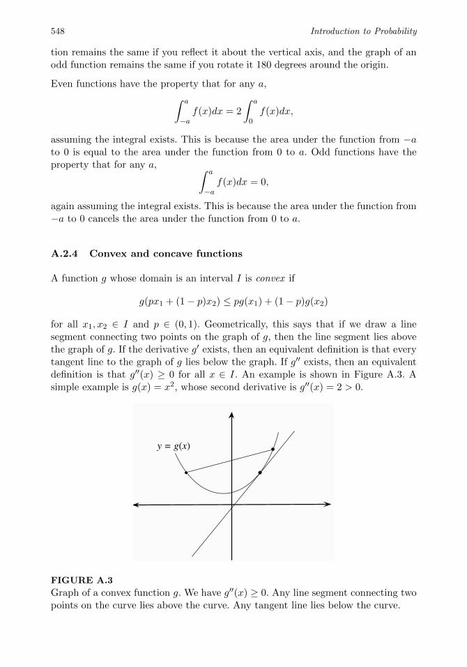
548 Introduction to Probability
tion remains the same if you reflect it about the vertical axis, and the graph of anodd function remains the same if you rotate it 180 degrees around the origin.
Even functions have the property that for any a,
Z a
�af(x)dx = 2
Z a
0
f(x)dx,
assuming the integral exists. This is because the area under the function from �ato 0 is equal to the area under the function from 0 to a. Odd functions have theproperty that for any a, Z a
�af(x)dx = 0,
again assuming the integral exists. This is because the area under the function from�a to 0 cancels the area under the function from 0 to a.
A.2.4 Convex and concave functions
A function g whose domain is an interval I is convex if
g(px1
+ (1� p)x2
) pg(x1
) + (1� p)g(x2
)
for all x1
, x2
2 I and p 2 (0, 1). Geometrically, this says that if we draw a linesegment connecting two points on the graph of g, then the line segment lies abovethe graph of g. If the derivative g0 exists, then an equivalent definition is that everytangent line to the graph of g lies below the graph. If g00 exists, then an equivalentdefinition is that g00(x) � 0 for all x 2 I. An example is shown in Figure A.3. Asimple example is g(x) = x2, whose second derivative is g00(x) = 2 > 0.
y = g(x)
FIGURE A.3
Graph of a convex function g. We have g00(x) � 0. Any line segment connecting twopoints on the curve lies above the curve. Any tangent line lies below the curve.

Math 549
A function g is concave if �g is convex. If g00 exists, then g is concave if and onlyif g00(x) 0 for all x in the domain. For example, g(x) = log(x) defines a concavefunction on (0,1) since g00(x) = �1/x2 < 0 for all x 2 (0,1).
A.2.5 Exponential and logarithmic functions
Exponential functions are functions of the form f(x) = ax for some number a > 0.If a > 1, the function is increasing, and if 0 < a < 1, the function is decreasing. Themost common exponential function we’ll work with is f(x) = ex, and a very usefullimit result to know is that ⇣
1 +x
n
⌘n! ex
as n ! 1, for any real number x. This has an interpretation in terms of a bankpaying compound interest on a deposit: as compounding occurs more and moretimes per year, the growth rate approaches exponential growth.
Here are some properties of exponential functions:
1. axay = ax+y.
2. axbx = (ab)x.
3. (ax)y = axy.
The inverse of an exponential function is a logarithmic function: for positive y, loga yis defined to be the number x such that ax = y. Throughout this book, when wewrite log y without explicitly specifying the base, we are referring to the naturallogarithm (base e).
Here are some properties of logarithms:
1. loga x+ loga y = loga xy.
2. loga xn = n loga x.
3. loga x = log xlog a .
A.2.6 Floor function and ceiling function
The floor function is defined by letting bxc be the greatest integer less than orequal to x. That is, it says to round down to an integer. For example, b3.14c = 3,b�1.3c = �2, and b5c = 5. (Some books denote the floor function by [x] but thisis bad notation since it does not suggest a corresponding notation for the ceilingfunction, and since square brackets are also used for other purposes.)
The ceiling function is defined by letting dxe be the smallest integer greater thanor equal to x. For example, d3.14e = 4, d�1.3e = �1, and d5e = 5.

550 Introduction to Probability
A.2.7 Factorial function and gamma function
The factorial function takes a positive integer n and returns the product of theintegers from 1 to n, denoted n! and read “n factorial”:
n! = 1 · 2 · 3 . . . n.
Also, we define 0! = 1. This convention makes sense since if we think of n! as thenumber of ways in which n people can line up, there is 1 way for n = 0 (this justmeans there is no one there, so the line is empty). It is also very helpful since, forexample, we can then say that n!/(n � 1)! = n for all positive integers n withoutrunning into trouble when n = 1.
The factorial function grows extremely quickly as n grows. A famous, useful ap-proximation for factorials is Stirling’s formula,
n! ⇡p2⇡n
⇣ne
⌘n.
The ratio of the two sides converges to 1 as n ! 1. For example, direct calculationgives 52! ⇡ 8.066⇥ 1067, while Stirling’s formula says 52! ⇡ 8.053⇥ 1067.
The gamma function � generalizes the factorial function to positive real numbers;it is defined by
�(a) =
Z 1
0
xae�xdx
x, a > 0,
and has the property that
�(n) = (n� 1)!
for all positive integers n. Also, �(1/2) =p⇡.
An important property of the gamma function, which generalizes the fact thatn! = n · (n� 1)!, is that
�(a+ 1) = a�(a)
for all a > 0. See Chapter 8 for more about the gamma function.
A.3 Matrices
Neo: What is the Matrix?Trinity: The answer is out there, Neo, and it’s looking for you, and it will findyou if you want it to.– The Matrix (film from 1999)

Math 551
A matrix is a rectangular array of numbers, such as
0
B@3 1/e
2⇡ 1
1
CA or
0
B@1 1 0
1 2 3
1
CA.
We say that the dimensions of a matrix are m by n (also written m ⇥ n) if it hasm rows and n columns (so the former example is 2 by 2, while the latter is 2 by 3).The matrix is called square if m = n. If m = 1, we have a row vector ; if n = 1, wehave a column vector.
A.3.1 Matrix addition and multiplication
To add two matrices A and B with the same dimensions, just add the correspondingentries, e.g.,
0
B@1 1 0
1 1 1
1
CA+
0
B@1 0 0
1 1 0
1
CA =
0
B@2 1 0
2 2 1
1
CA .
When we multiply an m by n matrix A by an n by r matrix B, we obtain anm by r matrix AB; note that matrix multiplication is only well-defined when thenumber of columns of A equals the number of rows of B. The row i, column j entryof AB is
Pnk=1
aikbkj , where aij and bij are the row i, column j entries of A andB, respectively. For example, here is how to multiply a 2 ⇥ 3 matrix by a 3 ⇥ 1vector:
0
B@1 2 3
4 5 6
1
CA
0
BBBBB@
7
8
9
1
CCCCCA=
0
B@1 · 7 + 2 · 8 + 3 · 9
4 · 7 + 5 · 8 + 6 · 9
1
CA =
0
B@50
122
1
CA .
Note that AB may not equal BA, even if both are defined. To multiply a matrix Aby a scalar, just multiply each entry by that scalar.
The transpose of a matrix A is the matrix whose row i, column j entry is the row j,column i entry of A. It is denoted by A0 and read as “A transpose” or “A prime”.The rows of A are the columns of A0, and the columns of A are the rows of A0. If Aand B are matrices such that the product AB is defined, then (AB)0 = B0A0.
The determinant of a 2 by 2 matrix
0
B@a b
c d
1
CA is defined to be ad � bc. Determi-
nants can also be defined for n by n matrices, in a recursive manner not reviewedhere.
552 Introduction to Probability
A.3.2 Eigenvalues and eigenvectors
An eigenvalue of an n⇥ n matrix A is a number � such that
Av = �v
for some n⇥1 column vector v, where the elements of v are not all zero. The vectorv is called an eigenvector of A, or sometimes a right eigenvector. (A left eigenvectorof A would be a row vector w satisfying wA = �w for some �.) This definition saysthat when A and v are multiplied, v just gets stretched by the constant �.
Some matrices have no real eigenvalues, but the Perron-Frobenius theorem tells usthat in a special case that is of particular interest to us in Chapter 11, eigenvaluesexist and have nice properties. Let A be a square matrix whose entries are nonnega-tive and whose rows sum to 1. Further assume that for all i and j, there exists k � 1such that the row i, column j entry of Ak is positive. Then the Perron-Frobeniustheorem says that 1 is an eigenvalue of A, 1 is in fact the largest eigenvalue of A,and there is a corresponding eigenvector whose entries are all positive.
A.4 Di↵erence equations
A di↵erence equation describes a sequence of numbers in a way that involves thedi↵erences between successive numbers in the sequence. For example, the di↵erenceequation
pi+1
� pi = r(pi � pi�1
)
describes a sequence of numbers pi whose di↵erences ai ⌘ pi�pi�1
form a geometricsequence with common ratio r. In fact, there are many such sequences, so thisdi↵erence equation actually describes an entire collection of sequences.
In this section we will describe how to solve equations of the form
pi = p · pi+1
+ q · pi�1
for some constants p and q; the previous equation was a special case of this form.The first step is to guess a solution of the form pi = xi. Plugging this into the above,we have
xi = p · xi+1 + q · xi�1,
which reduces to x = px2 + q or px2 � x + q = 0. This is called the characteristicequation, and the solution to the di↵erence equation depends on whether the char-acteristic equation has one or two distinct roots. If there are two distinct roots r
1
and r2
, then the solution is of the form
pi = ari1
+ bri2

Math 553
for some constants a and b. If there is only one distinct root r, then the solution isof the form
pi = ari + biri.
In our case, the characteristic equation has roots 1 and q/p, which are distinct ifp 6= q and are both equal to 1 if p = q. So we have
pi =
8>><
>>:
a+ b
✓q
p
◆i
, p 6= q,
a+ bi, p = q.
This is called the general solution of the di↵erence equation, since we have not yetspecified the constants a and b. To get a specific solution, we need to know twopoints in the sequence in order to solve for a and b.
A.5 Di↵erential equations
Di↵erential equations are the continuous version of di↵erence equations. A di↵eren-tial equation uses derivatives to describe a function or collection of functions. Forexample, the di↵erential equation
dy
dx= 3y
describes a collection of functions that have the following property: the instanta-neous rate of change of the function at any point (x, y) is equal to cy. This is anexample of a separable di↵erential equation because we can separate the x’s andy’s, putting them on opposite sides of the equation:
dy
y= 3dx.
Now we can integrate both sides, giving log y = 3x+ c, or equivalently,
y = Ce3x,
where C is any constant. This is called the general solution of the di↵erential equa-tion, and it tells us that all functions satisfying the di↵erential equation are of theform y = Ce3x for some C. To get a specific solution, we need to specify one pointon the graph, which allows us to solve for C.
Separable di↵erential equations are a special case. In general, it may not be possibleto rearrange the x’s and y’s to be on opposite sides, so there are additional methodsfor solving non-separable di↵erential equations, which we will not review here.

554 Introduction to Probability
A.6 Partial derivatives
If you can do ordinary derivatives, you can do partial derivatives: just hold all theother input variables constant except for the one you’re di↵erentiating with respectto. For example, let f(x, y) = y sin(x2+y3). Then the partial derivative with respectto x is
@f(x, y)
@x= 2xy cos(x2 + y3),
and the partial derivative with respect to y is
@f(x, y)
@y= sin(x2 + y3) + 3y3 cos(x2 + y3).
The Jacobian of a function which maps (x1
, . . . , xn) to (y1
, . . . , yn) is the n by nmatrix of all possible partial derivatives, given by
@y
@x=
0
BBBBB@
@y1
@x1
@y1
@x2
. . . @y1
@xn
......
...
@yn
@x1
@yn
@x2
. . . @yn
@xn
1
CCCCCA.
A.7 Multiple integrals
If you can do single integrals, you can do multiple integrals: just do more than oneintegral, holding variables other than the current variable of integration constant.For example,
Z1
0
Z y
0
(x� y)2dxdy =
Z1
0
Z y
0
(x2 � 2xy + y2)dxdy
=
Z1
0
(x3/3� x2y + xy2)
����y
0
dy
=
Z1
0
(y3/3� y3 + y3)dy
=1
12.
A.7.1 Change of order of integration
We can also integrate in the other order, dydx rather than dxdy, as long as we arecareful about the limits of integration. Since we’re integrating over all (x, y) with x

Math 555
and y between 0 and 1 such that x y, to integrate the other way we write
Z1
0
Z1
x(x� y)2dydx =
Z1
0
Z1
x(x2 � 2xy + y2)dydx
=
Z1
0
(x2y � xy2 + y3/3)
����1
x
dx
=
Z1
0
(x2 � x+ 1/3� x3 + x3 � x3/3)dx
=
✓x3/3� x2/2 + x/3� x4
12
◆ ����1
0
=1
12.
A.7.2 Change of variables
In making a change of variables with multiple integrals, a Jacobian is needed. Let’sstate the two-dimensional version, for concreteness. Suppose we make a change ofvariables (transformation) from (x, y) to (u, v), say with x = g(u, v), y = h(u, v).Then Z Z
f(x, y)dxdy =
Z Zf(g(u, v), h(u, v))
����@(x, y)
@(u, v)
���� dudv,
over the appropriate limits of integration, where���@(x,y)@(u,v)
��� is the absolute value of thedeterminant of the Jacobian. We assume that the partial derivatives exist and arecontinuous, and that the determinant is nonzero.
For example, let’s find the area of a circle of radius 1. To find the area of a region,we just need to integrate 1 over that region (so any di�culty comes from the limitsof integration; the function we’re integrating is just the constant 1). So the areais
ZZ
x2
+y21
1dxdy =
Z1
�1
Z p1�y2
�p1�y2
1dxdy = 2
Z1
�1
p1� y2dy.
Note that the limits for the inner variable (x) of the double integral can depend onthe outer variable (y), while the outer limits are constants. The last integral can bedone with a trigonometric substitution, but instead let’s simplify the problem bytransforming to polar coordinates: let
x = r cos ✓, y = r sin ✓,
where r is the distance from (x, y) to the origin and ✓ 2 [0, 2⇡) is the angle. TheJacobian matrix of this transformation is
556 Introduction to Probability
d(x, y)
d(r, ✓)=
0
B@cos ✓ �r sin ✓
sin ✓ r cos ✓,
1
CA
so the absolute value of the determinant is r(cos2 ✓ + sin2 ✓) = r. That is, dxdybecomes rdrd✓. So the area of the circle is
Z2⇡
0
Z1
0
rdrd✓ =
Z2⇡
0
1
2d✓ = ⇡.
For a circle of radius r, it follows immediately that the area is ⇡r2 since we canimagine converting our units of measurement to the unit for which the radius is1.
This may seem like a lot of work just to get such a familiar result, but it served asillustration and with similar methods, we can get the volume of a ball in any numberof dimensions! It turns out that the volume of a ball of radius 1 in n dimensions is
⇡n/2
�(n/2+1)
, where � is the gamma function (see Section A.2.7).
A.8 Sums
“So you’ve got to the end of our race-course?” said the Tortoise. “Even though itdoes consist of an infinite series of distances? I thought some wiseacre or anotherhad proved that the thing couldn’t be done?”“It can be done,” said Achilles; “It has been done! Solvitur ambulando. You see,the distances were constantly diminishing.”– Lewis Carroll [3]
There are several kinds of sums that come up frequently in probability.
A.8.1 Geometric series
A series of the formP1
n=0
xn is called a geometric series. For |x| < 1, we have
1X
n=0
xn =1
1� x.
The series diverges if |x| � 1. A series of the same form except with finitely manyterms is called a finite geometric series. For x 6= 1 the sum is
nX
k=0
xk =1� xn+1
1� x.
Math 557
A.8.2 Taylor series for ex
The Taylor series for ex is1X
n=0
xn
n!= ex, for all x.
A.8.3 Harmonic series and other sums with a fixed exponent
It is also useful to know thatP1
n=1
1/nc converges for c > 1 and diverges for c 1.For c = 1, this is called the harmonic series . The sum of the first n terms of theharmonic series can be approximated using
nX
k=1
1
k⇡ log(n) + �
for n large, where � ⇡ 0.577.
The sum of the first n positive integers isnX
k=1
k = n(n+ 1)/2.
For squares of integers, we havenX
k=1
k2 = n(n+ 1)(2n+ 1)/6.
For cubes of integers, amazingly, the sum is the square of the sum of the first npositive integers! That is,
nX
k=1
k3 = (n(n+ 1)/2)2.
A.8.4 Binomial theorem
The binomial theorem states that
(x+ y)n =nX
k=0
✓n
k
◆xkyn�k,
where�nk
�is a binomial coe�cient, defined as the number of ways to choose k objects
out of n, with order not mattering. An explicit formula for�nk
�in terms of factorials
is ✓n
k
◆=
n!
(n� k)!k!.
A proof of the binomial theorem is given in Example 1.4.17.

558 Introduction to Probability
A.9 Pattern recognition
Much of math and statistics is really about pattern recognition: seeing the essentialstructure of a problem, recognizing when one problem is essentially the same asanother problem (just in a di↵erent guise), noticing symmetry, and so on. We willsee many examples of this kind of thinking in this book. For example, suppose wehave the series
P1k=0
etke���k/k!, with � a positive constant. The e�� can be takenout from the sum, and then the structure of the series exactly matches up with thestructure of the Taylor series for ex. Therefore
1X
k=0
etke���k
k!= e��
1X
k=0
(�et)k
k!= e��e�e
t
= e�(et�1),
valid for all real t.
Similarly, suppose we want the Taylor series for 1/(1�x3) about x = 0. It would betedious to start taking derivatives of this function. Instead, note that this functionis reminiscent of the result of summing a geometric series. Therefore
1
1� x3=
1X
n=0
x3n,
valid for |x3| < 1 (which is equivalent to |x| < 1). What matters is the structure,not what names we use for variables!
A.10 Common sense and checking answers
It is very easy to make mistakes in probability, so checking answers is especiallyimportant. Some useful strategies for checking answers are (a) seeing whether theanswer makes sense intuitively (though as we have often seen in this book, probabil-ity has many results that seem counterintuitive at first), (b) making sure the answerisn’t a category error or a case of a biohazard, (c) trying out simple examples, (d)trying out extreme examples, and (e) looking for alternative methods to solve theproblem (including methods that might only give a bound or approximation, suchas using an inequality from Chapter 10 or running a simulation).
For example, here are some wrong arguments where the claim defies common sense.These illustrate the importance of doing sanity checks.
1.
“
Z1
�1
1
x2dx = (�x�1)
����1
�1
= �2.”

Math 559
This makes no sense intuitively, since 1/x2 is a positive quantity ; it wouldbe a miracle if its integral were negative!
2. “Let us findR
1
xdx using integration by parts. Let u = 1/x, dv = dx. Then
Z1
xdx = uv �
Zvdu = 1 +
Zx
x2dx = 1 +
Z1
xdx,
which implies 0 = 1 since we can cancel outR
1
xdx from both sides.”
3. What is wrong with the following “proof” that all horses are the samecolor? (This example is due to George Polya.) “Let n be the number ofhorses, and use induction on n to “prove” that in every group of n horses,all the horses have the same color. For the base case n = 1, there is onlyone horse, which clearly must be its own color. Now assume the claim istrue for n = k, and show that it is true for n = k+1. Consider a group ofk + 1 horses. Excluding the oldest horse, we have k horses, which by theinductive hypothesis must all be the same color. Excluding the youngesthorse, we have k horses, which again by the inductive hypothesis musthave the same color. Thus, all the horses have the same color.”
4. “There are 19 integers between 12 and 31 (inclusive) since 31 � 12 = 19.More generally, there are m�n numbers in the list n, n+1, . . . ,m if n andm are integers with m � n.” Such o↵-by-one errors are very common inmath and programming, but they can easily be avoided by checking simpleand extreme cases, e.g., there are 10 integers from 1 to 10 (inclusive) eventhough 10� 1 = 9.


B
R
B.1 Vectors
Command What it does
c(1,1,0,2.7,3.1) creates the vector (1, 1, 0, 2.7, 3.1)
1:100 creates the vector (1, 2, . . . , 100)
(1:100)^3 creates the vector (13, 23, . . . , 1003)
rep(0,50) creates the vector (0, 0, . . . , 0) of length 50
seq(0,99,3) creates the vector (0, 3, 6, 9, . . . , 99)
v[5] 5th entry of vector v (index starts at 1)
v[-5] all but the 5th entry of v
v[c(3,1,4)] 3rd, 1st, 4th entries of vector v
v[v>2] entries of v that exceed 2
which(v>2) indices of v such that entry exceeds 2
which(v==7) indices of v such that entry equals 7
min(v) minimum of v
max(v) maximum of v
which.max(v) indices where max(v) is achieved
sum(v) sum of the entries in v
cumsum(v) cumulative sums of the entries in v
prod(v) product of the entries in v
rank(v) ranks of the entries in v
length(v) length of vector v
sort(v) sorts vector v (in increasing order)
unique(v) lists each element of v once, without duplicates
tabulate(v) tallies how many times each element of v occurs
table(v) same as tabulate(v), except in table format
c(v,w) concatenates vectors v and w
union(v,w) union of v and w as sets
intersect(v,w) intersection of v and w as sets
v+w adds v and w entrywise (recycling if needed)
v*w multiplies v and w entrywise (recycling if needed)
561

562 Introduction to Probability
B.2 Matrices
Command What it does
matrix(c(1,3,5,7), nrow=2, ncol=2) creates the matrix
1 5
3 7
!
dim(A) gives the dimensions of matrix A
diag(A) extracts the diagonal of matrix A
diag(c(1,7)) creates the diagonal matrix
1 0
0 7
!
rbind(u,v,w) binds vectors u, v, w into a matrix, as rows
cbind(u,v,w) binds vectors u, v, w into a matrix, as columns
t(A) transpose of matrix A
A[2,3] row 2, column 3 entry of matrix A
A[2,] row 2 of matrix A (as a vector)
A[,3] column 3 of matrix A (as a vector)
A[c(1,3),c(2,4)] submatrix of A, keeping rows 1, 3 and columns 2, 4
rowSums(A) row sums of matrix A
rowMeans(A) row averages of matrix A
colSums(A) column averages of matrix A
colMeans(A) column means of matrix A
eigen(A) eigenvalues and eigenvectors of matrix A
solve(A) A�1
solve(A,b) solves Ax = b for x (where b is a column vector)
A %*% B matrix multiplication AB
A %^% k matrix power Ak (using expm package)

R 563
B.3 Math
Command What it does
abs(x) |x|exp(x) ex
log(x) log(n)
log(x,b) logb(n)
sqrt(x)
px
floor(x) bxcceiling(x) dxefactorial(n) n!
lfactorial(n) log(n!) (helps prevent overflow)
gamma(a) �(a)
lgamma(a) log(�(a)) (helps prevent overflow)
choose(n,k) binomial coe�cient�nk
�
pbirthday(k) solves birthday problem for k people
if (x>0) x^2 else x^3 x2 if x > 0, x3 otherwise (piecewise)
f <- function(x) exp(-x) defines the function f by f(x) = e�x
integrate(f, lower=0, upper=Inf) findsR10
f(x)dx numerically
optimize(f,lower=0,upper=5,maximum=TRUE) maximizes f numerically on [0, 5]
uniroot(f, lower=0, upper=5) searches numerically for a zero of f in [0, 5]
B.4 Sampling and simulation
Command What it does
sample(7) random permutation of 1, 2, . . . , 7
sample(52,5) picks 5 times from 1, 2, . . . , 52 (don’t replace)
sample(letters,5) picks 5 random letters of the alphabet (don’t replace)
sample(3,5,replace=TRUE,prob=p) picks 5 times from 1, 2, 3 with probabilities p (replace)
replicate(10^4,experiment) simulates 104 runs of experiment

564 Introduction to Probability
B.5 Plotting
Command What it does
curve(f, from=a, to=b) graphs the function f from a to b
plot(x,y) creates scatter plot of the points (xi, yi)
plot(x,y,type="l") creates line plot of the points (xi, yi)
points(x,y) adds the points (xi, yi) to the plot
lines(x,y) adds line segments through the (xi, yi) to the plot
abline(a,b) adds the line with intercept a, slope b to the plot
hist(x, breaks=b, col="blue") blue histogram of the values in x, with b bins suggested
par(new=TRUE) tells R not to clear the palette when we make our next plot
par(mfrow=c(1,2)) tells R we want 2 side-by-side plots (a 1 by 2 array of plots)
B.6 Programming
Command What it does
x <- pi sets x equal to ⇡
x>3 && x<5 Is x > 3 and x < 5? (TRUE/FALSE)
x>3 || x<5 Is x > 3 or x < 5? (TRUE/FALSE)
if (n>3) x <- x+1 adds 1 to x if n > 3
if (n==0) x <- x+1 else x <- x+2 adds 1 to x if n = 0, else adds 2
v<-rep(0,50); for (k in 1:50) v[k]<-pbirthday(k) solves birthday problem up to 50 people
B.7 Summary statistics
Command What it does
mean(v) sample mean of vector v
var(v) sample variance of vector v
sd(v) sample standard deviation of vector v
median(v) sample median of vector v
summary(v) min, 1st quartile, median, mean, 3rd quartile, max of v
quantile(v,p) pth sample quantile of vector v
cov(v,w) sample covariance of vectors v and w
cor(v,w) sample correlation of vectors v and w

R 565
B.8 Distributions
Command What it does
help(distributions) shows documentation on distributions
dbinom(k,n,p) PMF P (X = k) for X ⇠ Bin(n, p)
pbinom(x,n,p) CDF P (X x) for X ⇠ Bin(n, p)
qbinom(a,n,p) quantile min{x : P (X x) � a} for X ⇠ Bin(n, p)
rbinom(r,n,p) vector of r i.i.d. Bin(n, p) r.v.s
dgeom(k,p) PMF P (X = k) for X ⇠ Geom(p)
dhyper(k,w,b,n) PMF P (X = k) for X ⇠ HGeom(w, b, n)
dnbinom(k,r,p) PMF P (X = k) for X ⇠ NBin(r, p)
dpois(k,r) PMF P (X = k) for X ⇠ Pois(r)
dbeta(x,a,b) PDF f(x) for X ⇠ Beta(a, b)
dcauchy(x) PDF f(x) for X ⇠ Cauchy
dchisq(x,n) PDF f(x) for X ⇠ �2
n
dexp(x,b) PDF f(x) for X ⇠ Expo(b)
dgamma(x,a,r) PDF f(x) for X ⇠ Gamma(a, r)
dlnorm(x,m,s) PDF f(x) for X ⇠ LN (m, s2)
dnorm(x,m,s) PDF f(x) for X ⇠ N (m, s2)
dt(x,n) PDF f(x) for X ⇠ tn
dunif(x,a,b) PDF f(x) for X ⇠ Unif(a, b)
There are commands that are completely analogous to pbinom, qbinom, and rbinom
for the other distributions appearing in the above table. For example, pnorm, qnorm,and rnorm can be used to get the CDF, the quantiles, and random generation forthe Normal (note that the mean and standard deviation need to be provided as theparameters, rather than the mean and variance).
For the Multinomial, dmultinom can be used for calculating the joint PMF andrmultinom can be used for generating random vectors. For the Multivariate Normal,after installing and loading the mvtnorm package dmvnorm can be used for calculatingthe joint PDF and rmvnorm can be used for generating random vectors.


C
Table of distributions
Name Param. PMF or PDF Mean Variance
Bernoulli p P (X = 1) = p, P (X = 0) = q p pq
Binomial n, p�n
k
�pkqn�k, for k 2 {0, 1, . . . , n} np npq
FS p pqk�1, for k 2 {1, 2, . . . } 1/p q/p2
Geom p pqk, for k 2 {0, 1, 2, . . . } q/p q/p2
NBinom r, p�r+n�1
r�1
�prqn, n 2 {0, 1, 2, . . . } rq/p rq/p2
HGeom w, b, n(wk
)( b
n�k
)(w+b
n
), for k 2 {0, 1, . . . , n} µ = nw
w+b
(w+b�n
w+b�1
)nµ
n
(1� µ
n
)
Poisson � e
��
�
k
k!
, for k 2 {0, 1, 2, . . . } � �
Uniform a < b 1
b�a
, for x 2 (a, b) a+b
2
(b�a)
2
12
Normal µ,�2
1
�
p2⇡
e�(x�µ)
2
/(2�
2
) µ �2
Log-Normal µ,�2
1
x�
p2⇡
e�(log x�µ)
2
/(2�
2
), x > 0 ✓ = eµ+�
2
/2 ✓2(e�2 � 1)
Expo � �e��x, for x > 0 1/� 1/�2
Gamma a,� �(a)�1(�x)ae��xx�1, for x > 0 a/� a/�2
Beta a, b �(a+b)
�(a)�(b)
xa�1(1� x)b�1, for 0 < x < 1 µ = a
a+b
µ(1�µ)
a+b+1
Chi-Square n 1
2
n/2
�(n/2)
xn/2�1e�x/2, for x > 0 n 2n
Student-t n �((n+1)/2)pn⇡�(n/2)
(1 + x2/n)�(n+1)/2 0 if n > 1 n
n�2
if n > 2
567

Bibliography
[1] Donald J. Albers and Gerald L. Alexanderson. More Mathematical People:Contemporary Conversations. Academic Press, 1990.
[2] Steve Brooks, Andrew Gelman, Galin Jones, and Xiao-Li Meng. Handbook ofMarkov Chain Monte Carlo. CRC Press, 2011.
[3] Lewis Carroll. What the Tortoise Said to Achilles. Mind, 4(14):278–290, 1895.
[4] Jian Chen and Je↵rey S. Rosenthal. Decrypting classical cipher text usingMarkov chain Monte Carlo. Statistics and Computing, 22(2):397–413, 2012.
[5] William G. Cochran. The e↵ectiveness of adjustment by subclassification inremoving bias in observational studies. Biometrics, 1968.
[6] Persi Diaconis. Statistical problems in ESP research. Science, 201(4351):131–136, 1978.
[7] Persi Diaconis. The Markov chain Monte Carlo revolution. Bulletin of theAmerican Mathematical Society, 46(2):179–205, 2009.
[8] Persi Diaconis, Susan Holmes, and Richard Montgomery. Dynamical bias inthe coin toss. SIAM Review, 49(2):211–235, 2007.
[9] Bradley Efron and Ronald Thisted. Estimating the number of unseen species:How many words did Shakespeare know? Biometrika, 63(3):435, 1976.
[10] Bradley Efron and Ronald Thisted. Did Shakespeare write a newly-discoveredpoem? Biometrika, 74:445–455, 1987.
[11] Andrew Gelman, John B. Carlin, Hal S. Stern, David B. Dunson, Aki Vehtari,and Donald B. Rubin. Bayesian Data Analysis. CRC Press, 2013.
[12] Andrew Gelman and Deborah Nolan. You can load a die, but you can’t bias acoin. The American Statistician, 56(4):308–311, 2002.
[13] Andrew Gelman, Boris Shor, Joseph Bafumi, and David K. Park. Red State,Blue State, Rich State, Poor State: Why Americans Vote the Way They Do(Expanded Edition). Princeton University Press, 2009.
[14] Gerd Gigerenzer and Ulrich Ho↵rage. How to improve Bayesian reasoning with-out instruction: Frequency formats. Psychological Review, 102(4):684, 1995.
[15] Prakash Gorroochurn. Classic Problems of Probability. John Wiley & Sons,2012.
569

570 Bibliography
[16] Richard Hamming. You and your research. IEEE Potentials, pages 37–40,October 1993.
[17] David P. Harrington. The randomized clinical trial. Journal of the AmericanStatistical Association, 95(449):312–315, 2000.
[18] David J.C. MacKay. Information Theory, Inference and Learning Algorithms.Cambridge University Press, 2003.
[19] Oscar Mandel. Chi Po and the Sorcerer: A Chinese Tale for Children andPhilosophers. Charles E. Tuttle Company, 1964.
[20] T.J. Mathews and Brady E. Hamilton. Trend analysis of the sex ratio at birthin the United States. National Vital Statistics Reports, 53(20):1–17, 2005.
[21] Pierre Remond de Montmort. Essay d’Analyse sur les Jeux de Hazard. Quilau,Paris, 1708.
[22] John Allen Paulos. Innumeracy: Mathematical Illiteracy and Its Consequences.Macmillan, 1988.
[23] Horst Rinne. The Weibull Distribution: A Handbook. CRC Press, 2008.
[24] James G. Sanderson. Testing ecological patterns. American Scientist, 88:332–339, 2000.
[25] Nate Silver. The Signal and the Noise: Why So Many Predictions Fail—butSome Don’t. Penguin, 2012.
[26] Tom W. Smith, Peter Marsden, Michael Hout, and Jibum Kim. General so-cial surveys, 1972–2012. Sponsored by National Science Foundation. NORC,Chicago: National Opinion Research Center, 2013.
[27] Stephen M. Stigler. Isaac Newton as a probabilist. Statistical Science,21(3):400–403, 2006.
[28] Tom Stoppard. Rosencrantz & Guildenstern Are Dead. Samuel French, Inc.,1967.
[29] R.J. Stroeker. On the sum of consecutive cubes being a perfect square. Com-positio Mathematica, 97:295–307, 1995.
[30] Amos Tversky and Daniel Kahneman. Causal schemas in judgments under un-certainty. In Daniel Kahneman, Paul Slovic, and Amos Tversky, editors, Judg-ment under Uncertainty: Heuristics and Biases. Cambridge University Press,1982.
[31] Herbert S. Wilf. generatingfunctionology. A K Peters/CRC Press, 3rd edition,2005.

K16714
Developed from celebrated Harvard statistics lectures, Introduction to Probability provides essential language and tools for understanding statistics, randomness, and uncertainty. The book explores a wide variety of applications and examples, ranging from coincidences and paradoxes to Google PageRank and Markov chain Monte Carlo (MCMC). Additional application areas explored include genetics, medicine, computer science, and information theory.
The authors present the material in an accessible style and motivate concepts using real-world examples. Throughout, they use stories to uncover connections between the fundamental distributions in statistics and conditioning to reduce complicated problems to manageable pieces.
The book includes many intuitive explanations, diagrams, and practice problems. Each chapter ends with a section showing how to perform relevant simulations and calculations in R, a free statistical software environment.
Statistics Texts in Statistical Science
Joseph K. BlitzsteinJessica Hwang
Blitzstein • Hwang
Introduction to Probability
Introduction to Probability
Introduction to Probability
• Access online or download to your smartphone, tablet or PC/Mac• Search the full text of this and other titles you own• Make and share notes and highlights• Copy and paste text and figures for use in your own documents• Customize your view by changing font size and layout
WITH VITALSOURCE®
EBOOK
K16714_cover.indd 1 6/24/14 2:38 PM