wireless network algorithms, systems, and applications
TRANSCRIPT

EURASIP Journal on Wireless Communications and Networking
Wireless Network Algorithms, Systems, and Applications
Guest Editors: Benyuan Liu, Azer Bestavros, Jie Wang, and Ding-Zhu Du

Wireless Network Algorithms, Systems,and Applications

EURASIP Journal onWireless Communications and Networking
Wireless Network Algorithms, Systems,and Applications
Guest Editors: Benyuan Liu, Azer Bestavros, Jie Wang,and Ding-Zhu Du

Copyright © 2010 Hindawi Publishing Corporation. All rights reserved.
This is a special issue published in volume 2010 of “EURASIP Journal on Wireless Communications and Networking.” All articles areopen access articles distributed under the Creative Commons Attribution License, which permits unrestricted use, distribution, andreproduction in any medium, provided the original work is properly cited.

Editor-in-ChiefLuc Vandendorpe, Universite catholique de Louvain, Belgium
Associate Editors
Thushara Abhayapala, AustraliaMohamed H. Ahmed, CanadaFarid Ahmed, USACarles Anton-Haro, SpainAnthony C. Boucouvalas, GreeceLin Cai, CanadaYuh-Shyan Chen, TaiwanPascal Chevalier, FranceChia-Chin Chong, South KoreaNicolai Czink, AustriaSoura Dasgupta, USAR. C. De Lamare, UKIbrahim Develi, TurkeyPetar M. Djuric, USAAbraham O. Fapojuwo, CanadaMichael Gastpar, USAAlex B. Gershman, GermanyWolfgang H. Gerstacker, GermanyDavid Gesbert, France
Zabih F. Ghassemlooy, UKJean-marie Gorce, FranceChristian Hartmann, GermanyStefan Kaiser, GermanyGeorge K. Karagiannidis, GreeceChi Chung Ko, SingaporeNicholas Kolokotronis, GreeceRichard Kozick, USASangarapillai Lambotharan, UKVincent Lau, Hong KongDavid I. Laurenson, UKTho Le-Ngoc, CanadaTongtong Li, USAWei Li, USATongtong Li, USAZhiqiang Liu, USAStephen McLaughlin, UKSudip Misra, IndiaIngrid Moerman, Belgium
Marc Moonen, BelgiumEric Moulines, FranceSayandev Mukherjee, USAKameswara Rao Namuduri, USAAmiya Nayak, CanadaMonica Nicoli, ItalyClaude Oestges, BelgiumA. Pandharipande, The NetherlandsJordi Perez-Romero, SpainPhillip Regalia, FranceGeorge S. Tombras, GreeceAthanasios Vasilakos, GreecePing Wang, CanadaWeidong Xiang, USAXueshi Yang, USAKwan L. Yeung, Hong KongWeihua Zhuang, Canada

Contents
Wireless Network Algorithms, Systems, and Applications, Benyuan Liu, Azer Bestavros, Jie Wang,and Ding-Zhu DuVolume 2010, Article ID 589389, 2 pages
Load Balancing Routing with Bounded Stretch, Fan Li, Siyuan Chen, and Yu WangVolume 2010, Article ID 623706, 16 pages
NQAR: Network Quality Aware Routing in Error-Prone Wireless Sensor Networks, Jaewon Choi,Baek-Young Choi, Sejun Song, and Kwang-Hui LeeVolume 2010, Article ID 409724, 7 pages
On the Capacity of Hybrid Wireless Networks with Opportunistic Routing, Tan Le and Yong LiuVolume 2010, Article ID 202197, 9 pages
Centroid Localization of Uncooperative Nodes in Wireless Networks Using a Relative Span WeightingMethod, Christine Laurendeau and Michel BarbeauVolume 2010, Article ID 567040, 10 pages
Distributed Range-Free Localization Algorithm Based on Self-Organizing Maps, Pham Doan Tinh andMakoto KawaiVolume 2010, Article ID 692513, 9 pages
Fully Decentralized and Collaborative Multilateration Primitives for Uniquely Localizing WSNs,Arda Cakiroglu and Cesim ErtenVolume 2010, Article ID 605658, 7 pages
A Secure Localization Approach against Wormhole Attacks Using Distance Consistency, Honglong Chen,Wei Lou, Xice Sun, and Zhi WangVolume 2010, Article ID 627039, 11 pages
Scheduling Heterogeneous Wireless Systems for Efficient Spectrum Access, Lichun Bao and Shenghui LiaoVolume 2010, Article ID 736365, 14 pages
Efficient Scheduling of Pigeons for a Constrained Delay Tolerant Application, Jiazhen Zhou, Jiang Li,and Legand BurgeVolume 2010, Article ID 142921, 7 pages
Biologically Inspired Target Recognition in Radar Sensor Networks, Qilian LiangVolume 2010, Article ID 523435, 8 pages
ε-Net Approach to Sensor κ-Coverage, Giordano Fusco and Himanshu GuptaVolume 2010, Article ID 192752, 12 pages
SPM: Source Privacy for Mobile Ad Hoc Networks, Jian Ren, Yun Li, and Tongtong LiVolume 2010, Article ID 534712, 10 pages

Hindawi Publishing CorporationEURASIP Journal on Wireless Communications and NetworkingVolume 2010, Article ID 589389, 2 pagesdoi:10.1155/2010/589389
Editorial
Wireless Network Algorithms, Systems, and Applications
Benyuan Liu,1 Azer Bestavros,2 Jie Wang,1 and Ding-Zhu Du3
1 Department of Computer Science, University of Massachusetts Lowell, Lowell, MA 01854, USA2 Department of Computer Science, Boston University, MA 02215, USA3 Department of Computer Science, University of Texas at Dallas, TX 75083, USA
Correspondence should be addressed to Benyuan Liu, [email protected]
Received 3 February 2010; Accepted 3 February 2010
Copyright © 2010 Benyuan Liu et al. This is an open access article distributed under the Creative Commons Attribution License,which permits unrestricted use, distribution, and reproduction in any medium, provided the original work is properly cited.
Advances in wireless communication and networking tech-nologies proliferate ubiquitous infrastructure and ad hocwireless networks, enabling a wide variety of applicationsranging from environment monitoring to health care, fromcritical infrastructure protection to wireless security, toname just a few. The complexity and ramifications ofthe fast-growing number of mobile users and the varietyof services intensify the interest in developing principles,algorithms, design methodologies, and systematic evaluationframeworks for the next-generation wireless networks.
This special issue contains twelve papers selected fromsubmissions through open calls and the technical programof the Fourth Annual International Conference on WirelessAlgorithms, Systems, and Applications (WASA 2009), heldin Boston, Massachusetts, USA, during August 16–18, 2009.These papers highlight some of the current research interestsand achievements in the area of wireless communicationand networking. The topics include routing, localization,scheduling, target detection and coverage, and privacy inmobile ad hoc networks and sensor networks.
F. Li, S. Chen, and Y. Wang’s paper presents CircularSailing Routing (CSR), a routing protocol that provides aload-balanced routing for wireless networks. Their methodmaps the network onto a sphere via stereographic projectionand makes routing decision by “circular distance” on thesphere. They show that the distance traveled by packets inCSR is bounded above by a small constant factor of the lengthof the shortest path.
J. Choi, B.-Y. Choi, S. Song, and K.-H. Lee’s paperpresents a network quality-aware routing (NQAR) mech-anism to avoid noisy paths with high possibility of colli-sion, and thus save time from transmission backoffs andretransmissions. Their experiment results show that NQAR
effectively reduces the end-to-end delay and outperformsthe direct diffusion mechanisms under error-prone environ-ments.
T. Le and Y. Liu’s paper studies the capacity of hybridwireless networks with opportunistic routing. They presenta linear programming method to calculate the end-to-end throughput in a hybrid network. They show thatopportunistic routing can efficiently utilize base stations andachieve significantly higher capacity than traditional unicastrouting.
C. Laurendeau and M. Barbeau’s paper presents position-ing algorithms to estimate the position of an uncooperativetransmitter, based on the received signal strength of a singletarget message at a set of receivers with known coordinates.Their simulation results demonstrate that their algorithmscan effectively localize a target within the regulations stipu-lated for emergence services location accuracy.
P. D. Tinh and M. Kawai’s paper presents a distributedrange-free algorithm based on self-organizing maps. Theiralgorithm uses only connectivity information to determinenode locations. Utilizing the intersection areas between radiocoverages of neighboring nodes, the algorithm intends tomaximize the correlation between the neighboring nodes,which reduces the learning time significantly.
A. Cakiroglu and C. Erten’s paper provides fully decen-tralized but collaborative primitives for uniquely localizingwireless nodes with low computation and messaging require-ments. The primitives are based on construction of a specialorder for multilaterating the nodes within a cluster. Withrelatively small clusters and iteration counts, the proposedapproach can localize almost all the nodes that are uniquelylocalizable.

2 EURASIP Journal on Wireless Communications and Networking
H. Chen, W. Lou, X. Sun, and Z. Wang’s paper inves-tigates the impact of wormhole attacks on localization andpresents a consistency-based secure localization scheme. Thelocalization scheme includes wormhole attack detection,valid locator identification, and self-localization. The paperalso presents theoretical models to analyze the proposedlocalization scheme and evaluate its performance via simu-lation.
L. Bao and S. Liao’s paper addresses the spectrum scarcityproblem caused by the unbalanced utilization of radiofrequency bands in the current state of wireless spectrumallocations. The paper presents a spectrum-access schedulingto improve the spectrum utilization efficiency in hetero-geneous wireless systems. Their simulation results showthat spectrum-access scheduling is a feasible and promisingapproach to handling the spectrum scarcity problem.
J. Zhou, J. Li, and L. B. Burge III’s paper introducesthe notion of “pigeon networks,” motivated by an ancientpractice of employing pigeons for long-distance communi-cations, as a special type of delay-tolerant networks (DTNs)that use special-purpose message carriers for applicationssuch as disaster recovery. The paper presents efficientscheduling strategies for message carriers and analyzes thetraffic that can be supported under deadline constraints.
Q. Liang’s paper studies target recognition in radar sen-sor networks. Inspired by human’s innate ability to processand integrate information from disparate and network-based sources, the paper proposes two human-inspiredtarget detection algorithms for target-detection in radar-based sensor networks. Simulation results show that theproposed approaches perform well, whereas the existing two-dimensional construction algorithm does not work.
G. Fusco and H. Gupta’s paper studies the k-coverageproblem of wireless sensor networks. The goal is to activateminimum number of sensors to ensure that each target inthe area is covered by at least k sensors. This problem isNP complete. The authors present an algorithm with anapproximation ratio of O(logM) based on the extensionof the classical ε-net technique, where M is the number ofsensors in an optimal solution.
J. Ren, Y. Li, and T. Li’s paper deals with the sourceprivacy problem in mobile ad hoc networks (MANETs).Source privacy is a critical security requirement for mission-critical applications, especially for MANETs due to nodemobility and the lack of physical protection. The paperpresents communication protocols that provide source pri-vacy, end-to-end routing privacy, and message authenticity.The theoretical analysis and simulation show that theproposed schemes are efficient and can provide a highmessage delivery ratio.
Acknowledgments
We thank the authors for contributing papers to the specialissue. We are grateful to members of the program committeeand external referees of WASA 2009 for their work withindemanding time constraints. Finally, we would like tothank the editorial staff of EURASIP Journal on Wireless
Communications and Networks for their support in editingthis special issue.
Benyuan LiuAzer Bestavros
Jie WangDing-Zhu Du

Hindawi Publishing CorporationEURASIP Journal on Wireless Communications and NetworkingVolume 2010, Article ID 623706, 16 pagesdoi:10.1155/2010/623706
Research Article
Load Balancing Routing with Bounded Stretch
Fan Li,1 Siyuan Chen,2 and Yu Wang2
1 Beijing Laboratory of Intelligent Information Technology, School of Computer Science, Beijing Institute of Technology,Beijing 100081, China
2 Department of Computer Science, College of Computing and Informatics, The University of North Carolina at Charlotte,Charlotte, NC 28223, USA
Correspondence should be addressed to Yu Wang, [email protected]
Received 27 April 2009; Accepted 19 June 2009
Academic Editor: Benyuan Liu
Copyright © 2010 Fan Li et al. This is an open access article distributed under the Creative Commons Attribution License, whichpermits unrestricted use, distribution, and reproduction in any medium, provided the original work is properly cited.
Routing in wireless networks has been heavily studied in the last decade. Many routing protocols are based on classic shortest pathalgorithms. However, shortest path-based routing protocols suffer from uneven load distribution in the network, such as crowedcenter effect where the center nodes have more load than the nodes in the periphery. Aiming to balance the load, we propose anovel routing method, called Circular Sailing Routing (CSR), which can distribute the traffic more evenly in the network. Theproposed method first maps the network onto a sphere via a simple stereographic projection, and then the route decision is madeby a newly defined “circular distance” on the sphere instead of the Euclidean distance in the plane. We theoretically prove that fora network, the distance traveled by the packets using CSR is no more than a small constant factor of the minimum (the distance ofthe shortest path). We also extend CSR to a localized version, Localized CSR, by modifying greedy routing without any additionalcommunication overhead. In addition, we investigate how to design CSR routing for 3D networks. For all proposed methods, weconduct extensive simulations to study their performances and compare them with global shortest path routing or greedy routingin 2D and 3D wireless networks.
1. Introduction
Recently, wireless networks draw lots of attention due to theirpotential applications in various areas. They intrinsicallyhave many special characteristics and some unavoidablelimitations compared with traditional fixed infrastructurenetworks. Energy conservation and scalability are probablytwo most critical issues in designing protocols for largescale wireless networks because wireless devices are usuallypowered by batteries only with limited computing capabilityand the number of such devices could be very large.
Routing is one of the key topics in wireless networks andhas been well studied. Many routing protocols were proposedfor different purposes. For example, there are power efficientrouting for better energy efficiency, cluster-based routingfor better scalability and geographical routing to reduce theoverhead. In this paper, we are interested in designing a loadbalancing routing for large wireless networks. By spreadingthe traffic across the wireless network via the elaborate designof the routing algorithm, load balancing routing averages the
energy consumption. This extends the lifespan of the wholenetwork by extending the time until the first node is out ofenergy. Load balancing is also useful for reducing congestionhot spots thus reducing wireless collisions. Notice that thereare already several load balancing routing protocols [1–5]in literature. However, most of them try to dynamicallyadjust the routes to balance the real time traffic load basedon the knowledge of current load distribution (or currentremaining energy distribution), which is not very scalablefor large wireless networks. Here, we assume that individualnode does not know the current load and each node maywant to talk with all other nodes. We then address how todesign load balancing routing for all-to-all communicationscenario in a network.
Notice that most of routing protocols are based onshortest path algorithm where the packets are traveled viathe shortest path between a source and a destination. Evenfor the geographical localized routing protocols, such asgreedy routing, the packets usually follow the shortest pathswhen the network is dense and uniformly distributed. In

2 EURASIP Journal on Wireless Communications and Networking
(a) network topology
108
64
200
5
100
200
400
600
800
(b) load of all-to-all traffic
Figure 1: In a grid network, nodes in the center area have much heavier traffic load than nodes in other areas. Here, shortest path routing isapplied for all possible source-destination pairs.
greedy routing, the packet is forwarded to the neighborwhich is nearest to the destination. Taking the shortest pathcan achieve smaller delay or traveled distance, however itcan also lead to the uneven distribution of traffic load ina network. For example, nodes in the center of a networkwill have heavier traffic since most of the shortest routesgo through them. This is just like the transportation systemaround a big city where the downtown area is alwaysthe “hot spot.” Figure 1 shows a simulation result on thisscenario. The network is distributed on a 9× 9 grid, and thenetwork topology is shown in Figure 1(a). Consider an all-to-all communication scenario, that is, each node sends onepacket to all other nodes using Shortest Path Routing (SPR)algorithm. Figure 1(b) illustrates the cumulative traffic load(i.e., number of packets passing through) for each node. It isclear that nodes in the center area have much higher trafficload than nodes in other areas, therefore, nodes in the centerwill run out of their batteries very quickly.
To avoid the uneven load distribution of shortest pathrouting, we focus on designing routing protocols for wirelessnetworks which can achieve both small traveled distance andevenly distributed load in the network. Inspired from circularsailing (or called globular sailing), which sails on the arcof a great circle to make the shortest distance between twoplaces on the earth, we propose a new routing algorithmcalled Circular Sailing Routing (CSR). In CSR, wireless nodesin a 2D network are mapped to a sphere using reversedstereographic projection and the routing decision is madebased on a newly defined “circular distance” on the sphereinstead of the Euclidean distance in 2D plane. By doing so,the traffic from one side to another side of the network areawill avoid the center area. Thus, “hot spots” are eliminatedand the load is balanced.
However, there is no such thing as a free lunch. Whileload balancing routing protocol try to even the load distri-bution, it also uses longer routes than the shortest paths.In general, this means load balancing routing may needmore relaying nodes to deliver the packets thus leads to
large energy consumption. We treat the increase of pathlength as the cost of load balancing. We formally definethe competitiveness and stretch factor of any routing methodcompared to SPR. Given a routing method A, let PA(s, t)be the path found by A to connect the source node s andthe target node t. A routing method A is called l-competitiveif for every pair of nodes s and t, the total length of pathPA(s, t) is within a constant factor l of the length of theshortest path connecting s and t in the network. The constantfactor l is called stretch factor (or competitiveness factor) ofA. Then, we theoretically prove that for any networks, thestretch factor of CSR is bounded by max(π(1+ε)/2,π), whereε is a constant parameter only depends on the ratio betweenthe size of the network and the radius of the sphere used inCSR. In other words, CSR can guarantee the total distancetraveled by packets is constant competitive even in the worstcase.
Notice that recently Popa et al. [6] also proposed asimilar routing technique, called curveball routing (CBR),which maps the 2D network on a sphere using anotherstereographic projection method and route the packets basedon spherical distances between their virtual coordinates onthe sphere. However, the authors did not provide any formalstudy on the competitiveness of CBR, except claimed that“in the presented simulation, curveball routing increases theaverage path length by less than 7.5% compared to the greedypaths. Similarly, the longest path increases by 59%.”
CSR can be easily implemented based on either shortestpath routing or greedy routing. The only modification isa simple mapping calculation of the position informationand the computational overhead is negligible. There areno changes to the communication protocol and no anyadditional communication overhead.
The rest of the paper is organized as follows. In Section 2,we first introduce stereographic projection and different dis-tance metrics. Then we present our Circular Sailing Routing(CSR) protocol, prove its bounded stretch, and compare itsperformance with Shortest Path Routing via simulations in

EURASIP Journal on Wireless Communications and Networking 3
S(0, 0, 0)
N(0, 0, 2r)
O(0, 0, r)
r
m(x, y, 0)
m’(x’, y’, z’)
(a) Stereographic projection I
m’(x’, y’, z’)
S(0, 0, −r)
r
N(0, 0, r)
O(0, 0, 0)
m(x, y, 0)
(b) Stereographic projection II
O(0, 0, r)
S(0, 0, 0)
r
m(x, y, 0)
d
d
m’(x’, y’, z’)
N(0, 0, 2r)
(c) Lambert azimuthal equal-area projection
Figure 2: Projection from a sphere to a plane: one-to-one mappingsfrom a node m′ on a sphere S to a node m in a plane.
Section 3. In Section 4, we extend CSR to a localized version(LCSR) and compare its performance with greedy routing. InSection 5, we further extend CSR and LCSR to 3D versionsfor 3D networks. Two mapping methods for 3D CSR areproposed and theoretical analysis of their stretch factor areprovided. We review related work in Section 6 and concludeour paper in Section 7. A preliminary conference versionof this article appeared in [7]. This version introduces anew definition of circular distance which fixes a bug in theproof of Lemma 2, contains a new 3D projection method andstretch analysis for 3D networks, and provides better overallpresentation.
(a) 2D grid topology
S
10
5
2
(b) Size of sphere
210−1−2−2−10
120
0.51
1.52
2.53
3.54
(c) On sphere (r = 2)
50−5−5
050
2
4
6
8
10
(d) On sphere (r = 5)
1050−5−10−10−505100
5
10
15
20
(e) On sphere (r = 10)
Figure 3: The reversed stereographic projections of a grid network(9× 9 grid in a 20× 20 square area) to the sphere with various radii(2, 5, and 10).
2. Preliminaries
2.1. Stereographic Projection. In projective geometry, thestereographic projection [8] is a certain mapping (function)that projects a sphere onto a plane. Intuitively, it givesa planar picture of the sphere. The projection is definedon the entire sphere, except at one point—the projectionpoint. Where it is defined, the mapping is smooth and
4 EURASIP Journal on Wireless Communications and Networking
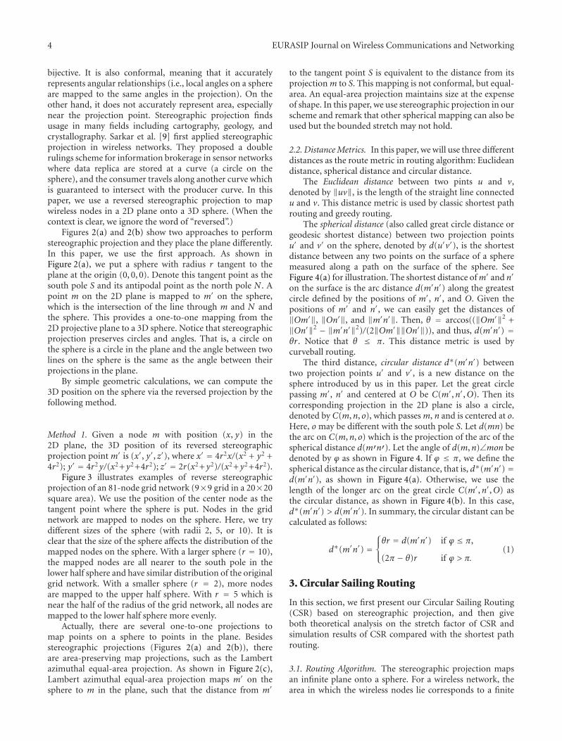
bijective. It is also conformal, meaning that it accuratelyrepresents angular relationships (i.e., local angles on a sphereare mapped to the same angles in the projection). On theother hand, it does not accurately represent area, especiallynear the projection point. Stereographic projection findsusage in many fields including cartography, geology, andcrystallography. Sarkar et al. [9] first applied stereographicprojection in wireless networks. They proposed a doublerulings scheme for information brokerage in sensor networkswhere data replica are stored at a curve (a circle on thesphere), and the consumer travels along another curve whichis guaranteed to intersect with the producer curve. In thispaper, we use a reversed stereographic projection to mapwireless nodes in a 2D plane onto a 3D sphere. (When thecontext is clear, we ignore the word of “reversed”.)
Figures 2(a) and 2(b) show two approaches to performstereographic projection and they place the plane differently.In this paper, we use the first approach. As shown inFigure 2(a), we put a sphere with radius r tangent to theplane at the origin (0, 0, 0). Denote this tangent point as thesouth pole S and its antipodal point as the north pole N . Apoint m on the 2D plane is mapped to m′ on the sphere,which is the intersection of the line through m and N andthe sphere. This provides a one-to-one mapping from the2D projective plane to a 3D sphere. Notice that stereographicprojection preserves circles and angles. That is, a circle onthe sphere is a circle in the plane and the angle between twolines on the sphere is the same as the angle between theirprojections in the plane.
By simple geometric calculations, we can compute the3D position on the sphere via the reversed projection by thefollowing method.
Method 1. Given a node m with position (x, y) in the2D plane, the 3D position of its reversed stereographicprojection point m′ is (x′, y′, z′), where x′ = 4r2x/(x2 + y2 +4r2); y′ = 4r2y/(x2+y2+4r2); z′ = 2r(x2+y2)/(x2+y2+4r2).
Figure 3 illustrates examples of reverse stereographicprojection of an 81-node grid network (9×9 grid in a 20×20square area). We use the position of the center node as thetangent point where the sphere is put. Nodes in the gridnetwork are mapped to nodes on the sphere. Here, we trydifferent sizes of the sphere (with radii 2, 5, or 10). It isclear that the size of the sphere affects the distribution of themapped nodes on the sphere. With a larger sphere (r = 10),the mapped nodes are all nearer to the south pole in thelower half sphere and have similar distribution of the originalgrid network. With a smaller sphere (r = 2), more nodesare mapped to the upper half sphere. With r = 5 which isnear the half of the radius of the grid network, all nodes aremapped to the lower half sphere more evenly.
Actually, there are several one-to-one projections tomap points on a sphere to points in the plane. Besidesstereographic projections (Figures 2(a) and 2(b)), thereare area-preserving map projections, such as the Lambertazimuthal equal-area projection. As shown in Figure 2(c),Lambert azimuthal equal-area projection maps m′ on thesphere to m in the plane, such that the distance from m′
to the tangent point S is equivalent to the distance from itsprojection m to S. This mapping is not conformal, but equal-area. An equal-area projection maintains size at the expenseof shape. In this paper, we use stereographic projection in ourscheme and remark that other spherical mapping can also beused but the bounded stretch may not hold.
2.2. Distance Metrics. In this paper, we will use three differentdistances as the route metric in routing algorithm: Euclideandistance, spherical distance and circular distance.
The Euclidean distance between two pints u and v,denoted by ‖uv‖, is the length of the straight line connectedu and v. This distance metric is used by classic shortest pathrouting and greedy routing.
The spherical distance (also called great circle distance orgeodesic shortest distance) between two projection pointsu′ and v′ on the sphere, denoted by d(u′v′), is the shortestdistance between any two points on the surface of a spheremeasured along a path on the surface of the sphere. SeeFigure 4(a) for illustration. The shortest distance ofm′ and n′
on the surface is the arc distance d(m′n′) along the greatestcircle defined by the positions of m′, n′, and O. Given thepositions of m′ and n′, we can easily get the distances of‖Om′‖, ‖On′‖, and ‖m′n′‖. Then, θ = arccos((‖Om′‖2 +‖On′‖2 − ‖m′n′‖2)/(2‖Om′‖‖On′‖)), and thus, d(m′n′) =θr. Notice that θ ≤ π. This distance metric is used bycurveball routing.
The third distance, circular distance d∗(m′n′) betweentwo projection points u′ and v′, is a new distance on thesphere introduced by us in this paper. Let the great circlepassing m′, n′ and centered at O be C(m′,n′,O). Then itscorresponding projection in the 2D plane is also a circle,denoted by C(m,n, o), which passes m, n and is centered at o.Here, o may be different with the south pole S. Let d(mn) bethe arc on C(m,n, o) which is the projection of the arc of thespherical distance d(m′n′). Let the angle of d(m,n)∠mon bedenoted by ϕ as shown in Figure 4. If ϕ ≤ π, we define thespherical distance as the circular distance, that is, d∗(m′n′) =d(m′n′), as shown in Figure 4(a). Otherwise, we use thelength of the longer arc on the great circle C(m′,n′,O) asthe circular distance, as shown in Figure 4(b). In this case,d∗(m′n′) > d(m′n′). In summary, the circular distant can becalculated as follows:
d∗(m′n′) =⎧⎨
⎩
θr = d(m′n′) if ϕ ≤ π,
(2π − θ)r if ϕ > π.(1)
3. Circular Sailing Routing
In this section, we first present our Circular Sailing Routing(CSR) based on stereographic projection, and then giveboth theoretical analysis on the stretch factor of CSR andsimulation results of CSR compared with the shortest pathrouting.
3.1. Routing Algorithm. The stereographic projection mapsan infinite plane onto a sphere. For a wireless network, thearea in which the wireless nodes lie corresponds to a finite

EURASIP Journal on Wireless Communications and Networking 5
n’
m’
mn
o
d∗(mn)d(mn)
ϕ
S(0, 0, 0)
N(0, 0, 2r)
O(0, 0, r)θd ∗
(m’n’)
d(m’n’)
(a) ϕ ≤ π
n’
m’
m
n
od(m
n)
ϕ
S(0, 0, 0)
N(0, 0, 2r)
O(0, 0, r)
θ
d ∗(m
’n’)
d∗ (mn)
d(m’n’)
(b) ϕ > π
Figure 4: The shortest distance between two points m′ and n′ on the sphere is the shorter segment of the greatest circle between m′ and n′.In this case, the circular distance is equal to the spherical distance, since ϕ < π. Otherwise, the circular distance is the longer segment of thegreatest circle.
1: Mapping: Map each node m(x, y, 0) in the 2D plane to anode m′(x′, y′, z′) on the sphere S (using Method 1).
2: New Metrics: For any existing link mn between twonodes m and n in the network, calculate the shortestcircular distance on the sphere between their projectednodes m′and n′ (i.e., d∗(m′n′)). We use d∗(m′n′) asthe cost of link, mn and call it circular distance.
3: Routing: Applying general shortest path routing withcircular distance as the routing metric, choose the routewith smallest total circular distance.
Algorithm 1: Circular sailing routing.
region of the plane. Let this region be called P. With theinformation of the network region, we can place the southpole S of a sphere S at the center of the network, whosecoordinate is (0, 0, 0). The radius r of S is an adjustableparameter for our proposed routing method. Here, weassume each node knows the radius r of the projectionsphere. This can be done via either a pre set before thedeployment or a broadcast operation after the deployment.Any point m(x, y, 0) in Pmaps to m′(x′, y′, z′) on the sphereS. It is a one-to-one mapping, where z′ ≤ k for some 0 <k < 2r. Here k is the z′ value of the highest projection on thesphere.
The basic idea of circular sailing routing is letting packetfollow the circular shortest paths on the sphere instead ofthe Euclidean shortest paths in 2D plane. Because there isno hot spot on the sphere where most of the circular shortestpaths must go through, we expect circular sailing routing canachieve better load balancing than shortest path routing. Thedetailed routing algorithm is given as Algorithm 1.
3.2. Analysis of Stretch Factor. In this section, we providetheoretical analysis on the stretch factor of CSR. Recall thata routing method A is called l-competitive or withl-boundedstretch if for every pair of nodes s and t, the total length ofpath PA(s, t) found by A is within l times of the shortest
path connecting s and t in the network. Hereafter, we call lthe Stretch Factor (SF).
3.2.1. Relationships among Distance Metrics. Before givingthe proof, we need to present some preliminaries forstereographic projection. Assume that the furthest wirelessnode is of distance D from the center (i.e., south pole of thesphere), then the z′ value of the highest projection on thesphere (i.e., the value of k) is
k = z′max = 2r
⎛
⎝D
√
D2 + (2r)2
⎞
⎠
2
= 2rD2
D2 + 4r2. (2)
As in [9], we choose r = D√ε/2, ε > 0, thus k = 2rε/(1 + ε).
Recall that circles on the sphere map to circles in theplane, thus the projection of a great circle on the sphere Sis also a circle in the plane. The spherical distance d(m′n′) isthe distance of the shorter arc C′ from a node m′ to a noden′ along the great circle on the surface of S. Let d(mn) be thedistance of an arc C between m and n along the projectionof C′ and the great circle in the plane (Figure 5). The circulardistance d∗(m′n′) is also the distance of the shorter arc fromm′ to n′ on the great circle (i.e., d∗(m′n′) = d(m′n′), asshown in Figure 4(a)) when ϕ ≤ π and is the distance of thelonger arc from m′ to n′ on the great circle when ϕ > π asshown in Figure 4(b). Let d∗(mn) be the distance of an arcin the plane between m and n along the projection of the arcof d∗(m′n′) as in Figure 4(b). Remember that ‖mn‖ denotesthe Euclidean distance between m and n in the plane. Thefollowing two lemmas show that the relationships amongd∗(m′n′), d(m′n′), and ‖mn‖. The major part (relationbetween d(m′n′) and d(mn)) of Lemma 1 and its proof arethe same with those of [9, Theorem 1]. However, we provideits proof for completeness.
Lemma 1. Consider any two nodes m′ and n′ on the sphere Swith their projections in the plane m and n, one has
‖mn‖ ≤ d(mn) ≤ (1 + ε)d(m′n′) ≤ (1 + ε)d∗(m′n′). (3)
Proof. First, since the Euclidean distance of two points isalways smaller than the distance along any arc passing them,

6 EURASIP Journal on Wireless Communications and Networking
mp q
C’
C
p’ q’
n
||mn||
d(mn)
S(0, 0, 0)
N(0, 0, 2r)
n’
m’O(0, 0, r)
d(m’n’)
p∗
Figure 5: The length of the projection d(mn) (or d∗(mn)) isbounded by the length of the shorter segment of great circle d(m′n′)(or d∗(m′n′)) on the sphere, that is, d(mn) ≤ d(m′n′)(1 + ε).
d∗(mn)C
‖mn‖ nm
o
ϕ
λ
Figure 6: The relationship between the arc distance d∗(mn) alonga circle and Euclidean distance ‖mn‖.
that is, ‖mn‖ ≤ d(mn). Second, the spherical distance onthe sphere is always smaller than the circular distance on thesphere, that is, d(m′n′) ≤ d∗(m′n′). Thus, we only need toprove d(mn) ≤ (2r/(2r − k))d(m′n′) = (1 + ε)d(m′n′).
Notice that it is one-to-one mapping between points onC′ and points on C · ∫ C′dx′ = d(m′n′), where dx′ is aminiature segment on C′. Similarly,
∫
Cdx = d(mn), wheredx is the projection of dx′ in the plane. See Figure 5 forillustration. p′q′ is a tiny segment on C′ with length dx′ →0, and dx′ = ‖p′q′‖. The projection of p′q′ is pq with thelength dx = ‖pq‖. Let p∗ be the projection of p′ on the linesegment NS. The z′ valued of p∗(or p′) is denoted by z′p∗ .Then
∥∥Np∗
∥∥
‖NS‖ = 2r − zp∗2r
. (4)
When dx′, dx → 0, that is, pq, p′q′ → 0, we can look pqand p′q′ as in the same plane (the plane defined by nodesN , p and q), more specifically, the two arcs pass through pqand p′q′ are concentric at north pole N . Then,
dx′dx
=∥∥p′q′
∥∥
∥∥pq
∥∥ =
∥∥Np′
∥∥
∥∥Np
∥∥ =
∥∥Np∗
∥∥
‖NS‖ = 2r − zp∗2r
. (5)
Because the highest value of zp∗ is k, we have
dx′
dx≥ 2r − k
2r= 2r − (2rε/(1 + ε))
2r= 1
1 + ε. (6)
Thus,
d(m′n′) =∫
C′dx′ ≥
∫
C
dx(1 + ε)
= d(m,n)(1 + ε)
. (7)
This finishes our proof.
Lemma 2. Consider any two points m′ and n′ on the spherewith their projections on the plane m and n, one has
d∗(m′n′) ≤ d∗(mn) ≤ π
2‖mn‖. (8)
Proof. Similar to the proof of Lemma 1, assume that dx′ is aminiature segment on C′ defined for d∗(m′n′) and dx is theprojection of dx′ in the plane. From the proof of Lemma 1,we know dx′/dx = (2r − z′p)/2r ≤ 1. Thus, dx′ ≤ dx, and
d∗(m′n′) =∫
C′dx′ ≤
∫
Cdx = d∗(mn). (9)
Figure 6 shows a top view of the arc C of d∗(mn) in the planeP. Arc C is a segment between m and n of a circle centered ato with the radius λ. Notice that o is not necessarily the centerO of the sphere. Then we have d∗(mn) = ϕλ and ‖mn‖ =2λ sin(ϕ/2). By the definition of circular distance, the angle ϕof the arc d∗(mn) is less or equal to π. Therefore,
d∗(mn)‖mn‖ = ϕλ
2λ sin(ϕ/2) = ϕ
2 sin(ϕ/2) . (10)
When ϕ = π, ϕ/2 sin(ϕ/2) reaches its maximum value,π/2. Thus, d∗(mn)/‖mn‖ ≤ π/2. This concludes the proof:d∗(m′n′) ≤ d∗(mn) ≤ (π/2)‖mn‖.
Notice that the relation in above lemma does not hold forspherical distance, since ϕ for spherical distance maybe largerthan π as shown in Figure 4(b). In other words, d(mn) couldbe larger than (π/2)‖mn‖.
3.2.2. Bounded Stretch Factor of CSR. Now we are ready toprove the main theorem of this paper about the stretch factorof CSR. We want to prove CSR can find a path whose lengthis within a small constant factor of the minimum even in theworst case scenario.
There are four paths we will use in the proof. Figure 7illustrates their definitions and the relationship among them.The dotted line in the plane represents the shortest pathgenerated by a shortest path routing connecting the sources and the destination t, denoted by PSPR(s, t). The dottedline on the sphere is the surface path connecting all theprojections on the sphere of each node along PSPR(s, t) usingthe circular distance, denoted by P
′SPR(s, t). The solid line
in the plane represents the path found by CSR protocol,denoted by PCSR(s, t) and the solid line on the sphere isthe surface path connecting all the projections of each nodealong PCSR(s, t), denoted by P
′CSR(s, t). Notice that, in any
two points along a path in the plane, the shortest distanceis the straight line connecting them, meanwhile the circulardistance of its projection on the sphere is a segment (an arc)of a great circle. For a path PA in the plane, we define ‖PA‖

EURASIP Journal on Wireless Communications and Networking 7
O(0,0,r)
ii−1v
i−1v’
iuui−1
iu’
v’i
i−1u’
P (s,t)CSR
SPR (s,t)P
SPRP’
(s,t)CSRP’t
t’
S(0,0,0)v
s
s’
N(0,0,2r)
(s,t)
Figure 7: The Euclidean path length of proposed CSR protocol isbounded by the Euclidean path length of shortest path routing.
as the summation of the Euclidian distance of each link inPA. For a path P′A on the sphere, we define d(P′A) as thesummation of the length of each arc in P′A.
Theorem 1. The stretch factor of CSR is bounded by (π/2)(1 +ε), that is,
‖PCSR(s, t)‖ ≤ π
2(1 + ε)‖PSPR(s, t)‖. (11)
Proof. Let PCSR(s, t) = v0, v1, v2, . . . , vn, where v0 = s andvn = t. Let the projection of PCSR(s, t) on the sphereP′CSR(s, t) = v′0, v′1, v′2, . . . , v′n. Similarly, let PSPR(s, t) =u0,u1,u2, . . . ,um, where u0 = s = v0 and um = t = vn.Let the projection of PSPR(s, t) on the sphere P′SPR(s, t) =u′0,u′1,u′2, . . . ,u′m, where u′0 = s′ = v′0 and u′m = t′ = v′n.s′ and t′ are the projections of source s and destination t onthe sphere. Notice that m may not equal to n.
From Lemma 1, we know ‖vi−1vi‖ ≤ (1 + ε)d∗(v′i−1v′i ),
therefore, ‖PCSR(s, t)‖ = ∑ni=1 ‖vi−1vi‖ ≤ ∑n
i=1(1 +ε)d∗(v′i−1v
′i ) = (1 + ε)d(P
′CSR(s, t)). According to the CSR
protocol, d(P′CSR(s, t)) ≤ d(P′SPR(s, t)) since P
′CSR(s, t) is the
shortest path using circular distance metric on the sphere.From Lemma 2, we have d∗(u′i−1u
′i ) ≤ (π/2)‖ui−1ui‖. Thus,
d(P′SPR(s, t)) = ∑ni=1 d
∗(u′i−1u′i ) ≤ ∑n
i=1(π/2)‖ui−1ui‖ =(π/2)‖PSPR(s, t)‖. Consequently, we have
‖PCSR(s, t)‖ ≤ (1 + ε)d(
P′CSR(s, t)
)
≤ (1 + ε)d(
P′SPR(s, t))
≤ π
2(1 + ε)‖PSPR(s, t)‖.
(12)
Theorem 1 gives a theoretical bound of the stretch factorof CSR protocol. It shows that the path length in CSR proto-col is not too much different from the shortest path routing.Since ε = D2/(4r2), with the adjustable parameter r (i.e., theradius of the sphere), we can control the stretch factor.
3.3. Simulation. We now evaluate the performance CSR viasimulations for both grid networks and random networks. Inboth cases, wireless nodes are distributed in a 20× 20 square
area. In CSR, the south pole of the sphere is tangent at thecenter of this area. Nodes in the area are mapped to nodes onthe sphere during the calculation of new metric. Here, we trydifferent sizes of the sphere (with radii 2, 5, or 10, as shownin Figure 3). It is clear that the size of the sphere affects thedistribution of the mapped nodes on the sphere.
Grid Networks. We first deploy the 81 nodes on a 9×9 grid ina 20×20 square area, and then set the transmission range R ofall nodes to 3. The resulted topology is shown in Figure 3(a).We compare the performance of the shortest path routing(SPR) and the circular sailing routing (CSR) under the all-to-all communication scenario. In other words, we assumeevery pair of nodes in the network has unit message tocommunicate. Figure 8(a) shows the distributions of eachnode’s traffic load for both SPR and CSR when the radiusof the sphere r = 5. It is clear that the load of CSR(Figure 8(a) (i)) is more evenly distributed than the load ofSPR (Figure 8(a) (ii)). The hot spot problem (center nodeswith highest load) is avoided in CSR. Figure 8(b) shows theaverage (Avg), maximum (Max) traffic load, and standarddeviation (STD) of traffic load for all nodes in the networkfor SPR and CSR with different radii. The average traffic loadof CSR are larger than SPR, especially when r = 2 (i.e.,most nodes are mapped to the upper half sphere). This isreasonable because the SPR has the least total traffic loadthan any other routing algorithms. Remember that SPR usesthe shortest path for each pair of nodes. When r = 5 and10, CSR has smaller maximum load and the STD of load ismuch less than SPR. Thus, CSR can balance the load trafficfor each node (s.t., the power consumptions of all nodes aremore even). These results meet our design objective well withonly a little bit more average traffic load. We also find thatwhen the nodes are mapped to the bottom half sphere (i.e.,r = 5), CSR has the best performance compared with othersizes of the sphere. When the radius is very large, the nodesare mapped to the area around the south pole, which hassimilar distribution with the original network. In such case,simulation results show that CSR’s performance is similar toSPR on the original network.
We also study the stretch factor (SF) of CSR.From Theorem 1, the distance traveled by CSR satisfies‖PCSR(s, t)‖ ≤ (π/2)(1 +ε)‖PSPR(s, t)‖, where ε = D2/(4r2).In our simulation settings, D = 10
√2. Thus, when r = 2, 5,
and 10, CF = 21.2, 4.7, and 2.4, respectively. We measurethe SF for each route generated by CSR in our simulation.Table 1 gives the average and maximum stretch factor (AvgSF and Max SF) of CSR with different radii. The simulationresults of SFs confirm our theoretical bounds. Actually thepractical SFs are much smaller than the bounds, and veryclose to 1. In other words, not only CSR has balanced trafficload but also the distance traveled by the packets is almostthe same as the minimum (the distance of the shortest path).
Random Networks. We also test the performance of CSRwith random networks. 81 nodes are randomly deployed inthe field with transmission range R set to 4. We run thesimulation for 100 random networks and take the average.

8 EURASIP Journal on Wireless Communications and Networking
Shortest path routing (SPR)
1050−5−10−10−505100
200
400
600
800
Shortest path routing (SPR)
10 5 0 −5 −10 −10 −5 0 5 100
200
400
600
800
Circular sailing routing (CSR) r = 5
(i) (ii)
(a)
CSR
r=
10C
SRr=
5C
SRr=
2SP
R
0
50
100
150
200
250
300
350
400
450
500Avg load
CSR
r=
10C
SRr=
5C
SRr=
2SP
R
0
200
400
600
800
1000
1200Max load
CSR
r=
10C
SRr=
5C
SRr=
2SP
R
0
50
100
150
200
250
300
350STD load
(b)
CSR
r=
10C
SRr=
5C
SRr=
2SP
R
0
50
100
150
200
250
300
350
400
450Avg load
CSR
r=
10C
SRr=
5C
SRr=
2SP
R
0
500
1000
1500
2000
2500Max load
CSR
r=
10C
SRr=
5C
SRr=
2SP
R
0
100
200
300
400
500
600STD load
(c)
Figure 8: Load of SPR and CSR: (a) traffic load of SPR and CSR (r = 5) on a 9× 9 grid; (b) comparison of traffic load of SPR (black), andCSR on a 9× 9 grid with r = 2 (green), 5 (blue), and 10 (red); (c) comparison of traffic load of SPR and CSR on 81-nodes random networkswith r = 2, 5, and 10.
1: For each neighbor v, node u maintains both a 2Dposition of v in the plane and a 3D position of itsprojection v′on the sphere S. Node u also maintainsits own 2D position and its projection’s 3D position.
2: While node u receives a packet with destination t do3: if‖ut‖ ≤ R, where R is the transmission range then4: Forward the packet to t directly and return.5: Map t to its projection t′ (i.e., get its 3D position).6: if ∃v, s.t., its projection v′ satisfies d∗(v′t′) < d∗(u′t′)
then7: Forward packet to node v with the minimum d∗(v′t′).8: else9: Simply drop the packet.
Algorithm 2: Localized circular sailing routing.
Figure 8(c) and the lower half of Table 1 summarize theperformance comparison of CSR for random networks. CSR(r = 5) has the best performance, that is, much smallermaximum load and load STD with little greater average loadand the average SF is very close to 1.0. CSR (r = 10) hassimilar performance with SPR because the mapped positionson the sphere are similar to those in the original network.
4. Localized Circular Sailing Routing
The geometric nature of wireless networks allows thepromising idea: localized routing protocols. In localizedrouting protocols, by assuming each node has positioninformation, the routing decision is made at each node byusing only local neighborhood information. It does not needthe dissemination of route discovery information, and norouting tables are maintained at each node. The most popu-lar localized routing is greedy routing [10] where the currentnode u always finds the next relay node v such that the dis-tance ‖t−v‖ is the smallest among all neighbors of u. Our cir-cular sail routing is easy to be extended to a localized versionwhich can achieve better load balancing than greedy routing.
4.1. Routing Algorithm. Similar to the classical greedy rout-ing, the Localized Circular Sailing Routing (LCSR) justforwards the packet to the neighbor whose projection isclosest to the projection of the destination on the sphere.Notice that each node only needs to know its neighbors’positions to make the routing decision. The detailed routingalgorithm is given in Algorithm 2.
If LCSR can find a neighbor to forward the packet ateach step, it will guarantee to reach the destination in finitesteps. The proof will be similar to the one for greedy routing.

EURASIP Journal on Wireless Communications and Networking 9
LCSR
r=
10LC
SRr=
5LC
SRr=
2G
reed
y
0
50
100
150
200
250Avg load
LCSR
r=
10LC
SRr=
5LC
SRr=
2G
reed
y
0
50
100
150
200
250
300
350
400Max load
LCSR
r=
10LC
SRr=
5LC
SRr=
2G
reed
y
0
10
20
30
40
50
60
70
80
90
100STD load
LCSR
r=
10LC
SRr=
5LC
SRr=
2G
reed
y
0
0.1
0.2
0.3
0.4
0.5
0.6
0.7
0.8
0.9
1Delivery ratio
(a) 3D Grid Network
LCSR
r=
10LC
SRr=
5LC
SRr=
2G
reed
y
0
20
40
60
80
100
120
140
160
180Avg load
LCSR
r=
10LC
SRr=
5LC
SRr=
2G
reed
y
0
50
100
150
200
250
300
350
400
450
500Max load
LCSR
r=
10LC
SRr=
5LC
SRr=
2G
reed
y
0
10
20
30
40
50
60
70
80
90STD load
LCSR
r=
10LC
SRr=
5LC
SRr=
2G
reed
y
0
0.1
0.2
0.3
0.4
0.5
0.6
0.7
0.8
0.9
1Delivery ratio
(b) 3D Random Network
Figure 9: Traffic load of Greedy Routing and LCSR: (a) traffic load of a 9× 9 grid network; (b) traffic load of 81-nodes random networks.
However, LCSR cannot always find the forwarding neighborsince it could fail into a local minimum where no suchneighbor v exists. To solve this problem, we can switch togreedy routing to find a forwarding neighbor who is nearestto destination in 2D plane. If the greedy routing cannot finda forwarding neighbor either, face routing in the plane canbe applied to get out of the local minimum as in [10, 11].If the packet reaches a location whose projection is closer tothe projection of the destination than the projection of theposition where the previous LCSR has failed, then LCSR isresumed.
4.2. Simulation. We test the performance of LCSR algorithmby using the same grid and random networks which areused in Section 3.3. We also assume all-to-all communica-tion in the networks. Classical greedy routing is used forcomparison. For simplicity, in the simulation, we implementLCSR without any recovery mechanisms, that is, LCSR(Algorithm 2) simply drops the packet at the local minimum.
Figures 9(a) and 9(b) show the performance comparisonof Greedy Routing and LCSR for the grid networks andrandom networks, respectively. Here, the data for randomnetworks is the average value of 50 random generatednetworks. It is clear that LCSR with r = 5 has the bestperformance, that is, smallest maximum traffic load and STDload for both gird and random networks. The delivery ratiois 100% and almost 100% for grid and random networks,respectively. For example for the gird network, the max loadof Greedy Routing is 400 while themax load of LCSR (r = 5)is 350, which is reduced about 12.5%. The STD load is alsodecreased by about 22.2%(from 90 to 70). The avg load ofLCSR (r = 5) and Greedy Routing are at the same value of208. Again, LCSR (r = 10) has very similar performance withgreedy routing, since the larger the sphere, the more alike thedistribution on the sphere to the original 2D distribution.
We also measure the Stretch Factor (SF) of CSR. Here,CF is the factor between the distance traveled by the packetin CSR and the distance traveled in greedy routing, if both
Table 1: Stretch factor (SF) of CSR (various sphere size).
Network topology Radius r Avg SF Max SF
Grid2 1.2202 2.6485
5 1.0085 1.2589
10 1.0000 1.0000
Random2 1.2150 3.2625
5 1.1122 1.0384
10 1.0135 1.0869
Table 2: Stretch factor (SF) of LCSR (various sphere size).
Network topology Radius r Avg SF Max SF
Grid2 1.0100 1.2761
5 1.0073 1.2071
10 1.0036 1.1380
Random2 1.1123 2.5688
5 1.0235 1.6125
10 1.0137 1.4656
routing methods can find a path between the source and thedestination. In the simulation, we randomly select 100 routes(10 source nodes and 10 destination nodes are randomlychosen ) and calculate the SF for each route. Table 2 givesthe results for both grid and random networks. Though wedo not have any proof of theoretical bounds, the SFs are verysmall in practice.
5. 3D Circular Sailing Routing
So far we consider routing in 2D network and how to map thenodes onto a sphere so that routing along the sphere can bal-ance the traffic load. The assumption of 2D network is some-what justified for applications where wireless devices aredeployed on earth surface and where the height of the net-work is much smaller than the transmission radius of a node.

10 EURASIP Journal on Wireless Communications and Networking
(a) 3D grid network
Traffic load for SPR at level 4
Traffic load for SPR at level 5
Traffic load for SPR at level 6
1050−5−10−10−505100
10002000
1050−5−10−10−505100
10002000
1050−5−10−10−50510
010002000
Traffic load for SPR at level 1
Traffic load for SPR at level 2
Traffic load for SPR at level 3
1050−5−10−10−505100
10002000
1050−5−10−10−505100
10002000
1050−5−10−10−50510
010002000
(b) Load of SPR
Figure 10: Uneven load in 3D network using SPR: (a) a 3D grid network with 216 nodes, and (b) the traffic load distribution of SPR at eachnode on each level.
However, 2D assumption may no longer be valid if a wirelessnetwork is deployed in space, atmosphere, or ocean, wherenodes of a network are distributed over a three-dimensional(3D) space and the difference in the third dimension istoo large to be ignored. In fact, recent interest in wirelesssensor networks hints at the strong need to design 3Dwireless networks. 3D wireless networks can be used in manyapplications, such as a underwater wireless sensor network[12] for 3D ocean environment observation or a 3D spacenetwork for space explorations [13]. In a 3D network, theproblem of uneven load distribution also exists. Figure 10(a)shows a 3D grid network with 6 × 6 × 6 nodes. Consider anall-to-all communication scenario, that is, each node sendsone packet to all other nodes using shortest path routingprotocol. Figure 10(b) illustrates the cumulative node traffic(i.e., number of packets passing through) for each node.Clearly, the center nodes of each level have higher load andthe two middle levels have much higher load than the top andbottom levels. Therefore, nodes in the center or in the middlelevels may run out of their batteries very quickly. To avoidthe uneven load distribution of shortest path routing, we arealso interested in how to extend the circular sailing routingto 3D wireless networks. To the best of our knowledge, our3D method (3D-CSR) is the first one to target at the designof load balancing routing in 3D wireless networks.
Fortunately, the idea of circular sailing routing can alsobe extended to 3D. Instead of mapping a plane to the surfaceof a sphere, 3D-CSR maps wireless nodes in a 3D region tothe surface of a 3D or 4D sphere.
5.1. One-to-One Projection Methods. We propose two projec-tion methods to map the nodes in 3D Euclidean space to asphere (either a 3D sphere or a 4D sphere).
Projection Method 1: Projection on 3D Sphere. For a 3Dwireless network, wireless nodes are distributed in a finite3D region R (e.g., a cube). With the information of thenetwork region, we can place the center O of a 3D sphere atthe center of the network, whose coordinate is (0, 0, 0). Theradius r of the 3D sphere is again an adjustable parameter.Any point m(x, y, z) in R maps to m′(x′, y′, z′,φ) on the 3Dsphere. Here (x′, y′, z′) is the 3D position of the projectionnodem′, and φ is the Euclidean distance fromm to the centerO. As shown in Figure 11(a), m′ is the intersection point ofthe 3D sphere and line mO. Sometimes the node is inside thesphere as node n in Figure 11(a). It is easy to show that thevirtual coordinates of m′ can be computed by the following
equations: x′ = (r/√
x2 + y2 + z2)x, y′ = (r/√
x2 + y2 + z2)y,
z′ = (r/√
x2 + y2 + z2)z, and φ =√
x2 + y2 + z2. Notice

EURASIP Journal on Wireless Communications and Networking 11
O(0, 0, 0)
nm’
m
n’ d ∗(m
’n’)
(a)
O(0, 0, 0)
n
m’(n’)
m
d∗ (m
’n’)
(b)
S(0, 0, 0, 0)
N(0, 0, 0, 2r)
O(0, 0, r)
r
m(x, y, z)
m’(x’, y’, z’, w’)
4D sphere
3D hyperplane
(c)
Figure 11: (a)-(b) Projection Method 1: from a node m(x, y, z)in 3D space to a node m′(x′, y′, z′,φ) on the 3D sphere. Thereare two cases for the calculation of spherical distance d∗(m′,n′):(a) m′ and n′ are different points on the sphere; (b) m′ and n′
are the same point on the sphere. (c) Projection Method 2—Stereographic Projection: an one-to-one mapping from a node min a 3D hyperplane to a node m′ on a 4D sphere.
that we need to specially deal with the node O(0, 0, 0) toguarantee that the projection is a one-to-one mapping. Here,we force to map it to the north pole with virtual coordinates(0, 0, r, 0).
To calculate the circular distance d∗(m′n′) between twoprojections m′ and n′, there are two cases as shown inFigures 11(a) and 11(b). If m′ and n′ are in differentpositions on the sphere (Figure 11(a)), d∗(m′n′) is theshortest surface distance on the sphere, which can becomputed by d∗(m′n′) = r arccos((‖Om′‖2 + ‖On′‖2 −‖m′n′‖2)/(2‖Om′‖‖On′‖)). In the second case, m′ and n′
are at the same point on the sphere (Figure 11(b)), then wecalculate d∗(m′n′) as the Euclidean distance between nodesm and n, that is, d∗(m′n′) = ‖mn‖ = |φm − φn|.
Projection Method 2: Projection on 4D Sphere. In the secondprojection method, we still use the stereographic projectionto map the nodes in 3D networks to a 4D sphere. Stere-ographic projection can be extended to high-dimensionalspace and sphere. Here, we use it to map a 3D region (a 3Dhyperplane) onto a 4D sphere. A 4D sphere (also called 3-sphere in math), often written as S3, is the set of points in4-dimensional Euclidean space which are at distance r froma fixed point of that space. This fixed point is the center ofthe 4D sphere. Stereographic projection is conformal in anydimension, that is, it preserves the angles at which curvescross each other and also preserves circles. Therefore, a circleon the sphere is also a circle in the plane (or hyperplane).As shown in Figure 11(c), we put a 4D sphere with radius rtangent to the 3D hyperplane at the center of the network.Denote this tangent point as the south pole S(0, 0, 0, 0) ofthe 4D sphere and its antipodal point as the north poleN(0, 0, 0, 2r). This 4D sphere can be defined as x2 + y2 +z2 + (w − r)2 = r2. A point m(x, y, z) in the 3D hyperplaneis mapped to m′(x′, y′, z′,w′) on the 4D sphere, which is theintersection of the linemN with the 4D sphere. This providesa one-to-one mapping of the 3D projective hyperplane to a4D sphere. It is easy to show that the virtual coordinates ofm′
can be computed by the following equations: x′ = 4r2x/(x2 +y2 + z2 + 4r2), y′ = 4r2y/(x2 + y2 + z2 + 4r2), z′ = 4r2z/(x2 +y2 + z2 + 4r2), and w′ = 2r(x2 + y2 + z2)/(x2 + y2 + z2 + 4r2).
Geodesics are curves on a surface which give the shortestdistance between two points. They are generalization of theconcept of a straight line in the plane. For all spheres, thegeodesics are great circles. For any two nodes m and n in 3Dnetwork, the geodesic of its projection m′ and n′ on the 4Dsphere is d(m′n′) = rθ where θ = ∠m′On′ = arccos((x′mx
′n +
y′my′n + z′mz
′n + (w′m − r)(w′n − r))/r2) . Similar to 2D case, we
can then define our circular distance as follows,
d∗(m′n′) =⎧⎨
⎩
θr = d(m′n′) if ϕ ≤ π,
(2π − θ)r if ϕ > π,(13)
where ϕ = ∠mon in 3D space.
5.2. Routing Algorithm. All the routing algorithms (3D-CSRor 3D-LCSR) in 3D networks are the same as 2D-CSR and2D-LCSR (Algorithms 1 and 2), except for the projectionmethod and the definition of circular distance d∗(m′n′).In 3D CSR, each node u uses the above projection method(either method 1 or method 2) to compute the virtualcoordinates of itself and its neighbors on the sphere. For anylink uv, 3D-CSR can calculate the circular distance on thesphere between projected nodes u′ and v′ (i.e., d∗(u′v′)) anduse it as the routing metric. For 3D-LCSR, current node uchooses the neighbor v if d(v′t′) is the minimum among allneighbors.
5.3. Analysis of Stretch Factor. Similar to CSR in 2D networks,3D CSR can balance the load and eliminates the crowed

12 EURASIP Journal on Wireless Communications and Networking
center effect, but at the same time it uses longer path betweenthe source and the destination than the shortest path routing.This may increase the total delay of the packet delivery.Therefore, we now theoretically study the stretch factor of3D CSR with Projection Method 1 or Projection Method 2.
Theorem 2. The stretch factor of 3D CSR with ProjectionMethod 1 (3D-CSR-I) is not bounded.
Proof. We prove the theorem by constructing an exam-ple where CSR has a arbitrary large SF. See Figure 12for illustration. The network only has four nodes: s, t,m, and n with coordinates (ε, 0, 0), (0, ε, 0), (0, 0, ε), and((√
2/2)r, (√
2/2)r, 0), respectively. Here, ε could be anarbitrary small number. The network only has four links:sm, sn, tm, and tn. From s to t, there are two paths,s → m → t and s → n → t. Applying the firstprojection method (Projection Method 1), 3D-CSR-I getsthe positions of the projected nodes: s′(r, 0, 0, ε), t′(0, r, 0, ε),m′(0, 0, r, ε), and n′((
√2/2)r, (
√2/2)r, 0, r). Since d∗(s′n′) +
d∗(n′t′) = πr/2, which is smaller than d∗(s′m′)+d∗(m′t′) =πr, 3D-CSR-I will chose node n to be the relay node forpackets between s and t. The total distance of PCSR(s, t) =‖sn‖ + ‖nt‖ = 2
√
((√
2/2)r − ε)2+ ((
√2/2)r)
2. However,
the length of shortest path PSPR(s, t) = ‖sm‖ + ‖mt‖ =2√
2ε. Thus, the stretch factor l = PCSR(s, t)/PSPR(s, t) =√
(((√
2/2)r − ε)2+ ((
√2/2)r)
2)/2ε2. When ε is arbitrary
small, l can be arbitrary large.
Theorem 2 implies that 3D-CSR-I may use an arbitrarylonger path than the shortest path in the worst case.Fortunately, the worst case seldom occurs in a randomnetwork. Later, our simulation results show that the SF of3D-CSR-I is not very large for grid or random networks inpractice.
For the stretch factor of CSR with Projection Method2 (3D-CSR-II), the analysis is very similar to the case of2D CSR. Recall that stereographic projection is conformalin any dimension. Using the similar proofs (as we did forLemma 1, Lemma 2, and Theorem 1), we can prove thefollowing theorem.
Theorem 3. The stretch factor of 3D CSR with ProjectionMethod 2 (3D-CSR-II) is bounded by (π/2)(1 + ε), that is,
‖PCSR(s, t)‖ ≤ π
2(1 + ε)‖PSPR(s, t)‖. (14)
The only difference in the proofs is in 2D case the nodesin the 2D network plane are projected onto a 3D sphere andin 3D case the nodes in the 3D hyperplane are projectedonto a 4D sphere. Theorem 1 shows that the path length of3D-CSR-II protocol is not too much different from the pathlength of the shortest path routing.
5.4. Simulation. We now evaluate the performance of 3D-CSR and 3D-LCSR via extensive simulations for both 3Dgrid networks and 3D random networks in a 20 × 20 × 20cubic area. Again, we compare their performance under
m’
x
y
z
Os
s’m
t’n(n’)
tε
ε
ε
Figure 12: Illustration for the proof of unbounded SF for CSR withProjection Method 1.
Table 3: Stretch factor (CF) of CSR (various sphere size).
Networkr
Avg SF Max SFtopology 3D-CSR-I 3D-CSR-II 3D-CSR-I 3D-CSR-II
Grid3 1.1554 1.0116 6.6569 1.3314
5 1.1438 1.0019 6.6569 1.1716
15 1.1245 1.0000 3.8284 1.0000
Random3 1.0809 1.0432 2.8972 1.6342
5 1.1125 1.0245 3.1463 1.3987
15 1.1076 1.0124 2.6744 1.3462
the all-to-all communication scenario. Hereafter, we use3D-CSR-I/3D-LCSR-I to denote the routing methods withProjection Method 1 (mapping nodes on a 3D sphere) and3D-CSR-II/3D-LCSR-II to denote the routing methods withProjection Method 2 (mapping nodes on a 4D sphere).
5.4.1. CSR versus SPR. For grid network, 216 wireless nodesare distributed in 6 × 6 × 6 grids (see Figure 10(a)). Thetransmission range (Tr) is set to 4.5. For 3D randomnetworks, 100 nodes are randomly distributed in the 20×20×20 cube with each node’s Tr set to 6. We run the simulationfor 100 random networks and take the average. For both gridand random networks, we try different sizes of the sphere(with radii 3, 5, and 15). The furthest node is of distanceD = 10
√2 = 14.1 from the center of the network cube (or
projection sphere). When r = 15, the projection sphere is alittle bit larger than the network cube.
Figure 13 demonstrates the average (Avg), maximum(Max) traffic load, and standard deviation (Std) of load forSPR, 3D-CSR-I and 3D-CSR-II with different sphere sizes(r = 3, 5, and 15) for the grid and random networks.The leftmost bar of each sub-graph represents the ShortestPath Routing (SPR) method, the red bars represent 3D-CSR-I and blue bars represent 3D-CSR-II. The averageload of 3D-CSR-I is larger than SPR. However, 3D-CSR-II has even smaller average load than SPR especially forrandom networks. All CSR algorithms have much smallermaximum load and Std of load than SPR, for example, the

EURASIP Journal on Wireless Communications and Networking 13
Table 4: Stretch factor (SF) and delivery ratio of LCSR (various sphere size).
Network Topology Radius rAvg SF Max SF Delivery ratio
3D-LCSR-I 3D-LCSR-II 3D-LCSR-I 3D-LCSR-II Greedy 3D-LCSR-I 3D-LCSR-II
Grid3 1.0392 1.0308 1.5892 1.3060
1.00001.0000 1.0000
5 1.0318 1.0479 1.3060 1.3060 0.9960 1.0000
15 1.0368 1.0308 1.3060 1.3060 1.0000 1.0000
Random3 1.0613 1.0592 2.9016 3.2485
0.98350.9533 0.9165
5 1.0621 1.0601 2.4369 2.4265 0.9487 0.9529
15 1.0597 1.0603 2.7630 2.4967 0.9687 0.9863
r=
15
r=
5
r=
3
0
100
200
300
400
500
600
700
800
900Avg load
r=
15
r=
5
r=
3
0
200
400
600
800
1000
1200
1400
1600
1800
2000Max load
r=
15
r=
5
r=
3
0
50
100
150
200
250
300
350
400
450STD load
(a) 3D Grid Network
r=
15
r=
5
r=
3
0
50
100
150
200
250
300
350
400Avg load
r=
15
r=
5
r=
3
0
200
400
600
800
1000
1200
1400
1600
1800Max load
r=
15
r=
5
r=
3
0
50
100
150
200
250
300
350STD load
(b) 3D Random Network
Figure 13: Traffic load comparison among SPR, 3D-CSR-I and 3D-CSR-II with radii r = 3, 5, and 15: (a) traffic load of a 63 gridnetwork; (b) traffic load of 100-nodes random networks.
maximum load of 3D-CSR-II (r = 5) for grid network hasdecreased about 40.9% compared with SPR (from 1978.0 to1050.0); and the Std of 3D-CSR-I (r = 3) has about 55.4%deduction compared with SPR (from 423.4 to 188.9). Thus,our simulation results show that 3D-CSR can achieve betterload balancing than SPR.
r=
15
r=
5
r=
3
0
20
40
60
80
100
120Avg load
r=
15
r=
5
r=
3
0
50
100
150
200
250
300
350Max load
r=
15
r=
5
r=
3
0
10
20
30
40
50
60STD load
(a) 3D Grid Network
r=
15
r=
5
r=
3
0
10
20
30
40
50
60
70
80
90
100Avg load
r=
15
r=
5
r=
3
0
50
100
150
200
250Max load
r=
15
r=
5
r=
3
0
5
10
15
20
25
30
35STD load
(b) 3D Random Network
Figure 14: Traffic load comparison among greedy routing, 3D-LCSR-I and 3D-LCSR-II with radii r = 3, 5 and 15: (a) traffic loadof a 3D grid (4×4×4); (b) traffic load of 64-nodes random network.
We also study the stretch factor (SF) of CSR by measuringthe SF of each route generated by CSR in our simulation.Table 3 gives the average and maximum stretch factor (AvgSF and Max SF) of CSR with various radii. Remember that3D-CSR has unbounded SF in theory. As shown in Table 3,Max SFs of 3D-CSR-I (r = 3 and 5) for grid networks

14 EURASIP Journal on Wireless Communications and Networking
are around 6.6 which are much larger than the Max SFsof 3D-CSR-II. From Theorem 1, the distance traveled by3D-CSR-II satisfies ‖PCSR(s, t)‖ ≤ (π/2)(1 + ε)‖PSPR(s, t)‖,where ε = D2/(4r2). In our simulation settings, D = 10
√2.
Thus, when r = 3, 5, and 15, respectively, SF bounds are10.3, 4.7, and 1.9. The simulation results of SFs confirm ourtheoretical bounds of 3D-CSR-II. Actually the practical SFsare much smaller than the bounds, and very close to 1 (from1.00 to 1.64). In other words, not only 3D CSR has balancedtraffic load but also the distance traveled by the packets isalmost the same as the minimum.
5.4.2. LCSR versus Greedy. We then study the performanceof 3D LCSR via 3D grid and random networks. For gridnetwork, we use a network with 64 nodes in a 4× 4× 4 gridsand set Tr to 8. For random network, we generate 50 randomnetworks with 64 nodes in a 203 cube and set Tr to 8. For allresults, we take the average of these 50 networks.
Figure 14 shows the performance comparison of greedyrouting, 3D-LCSR-I and 3D-LCSR-II for the grid and ran-dom networks. The leftmost bar of each subgraph representsthe greedy routing method, red bars represent 3D-LCSR-I,and blue bars represent 3D-LCSR-II. For the grid network,3D-LCSR-I has larger maximum load than greedy algorithmfor all radii, but 3D-LCSR-II has much better performancethan greedy, that is, almost the same average load with muchsmaller maximum load and Std of load. For example, the Stdof load for 3D-LCSR-II (r = 3) has decreased dramaticallyfrom 30.0 to 9.6 (about 68%). In the scenario of randomnetworks, 3D-LCSR-I and 3D-LCSR-II both have similaraverage load to greedy routing, and their maximum load andStd of load are smaller than greedy routing.
We measure the SFs of 3D LCSR compared with greedyrouting method by randomly selecting 100 node pairs andcalculating the SF for each successful route. Table 4 providesthe results for both grid and random networks. Though wedo not have any theoretical bounds for 3D LCSR, the SFs arevery small in practice, that is, ranged from 1.03 to 3.25. Thistable also gives the delivery ratios. The delivery ratios of 3D-LCSR-II and -I are 100% and almost 100%, respectively, forgrid network with different radii. For the random networks,the delivery ratios of both 3D-LCSR-II and -I are still veryhigh (more than 91%).
6. Related Work
Load balancing routing protocols has been studied recently.Most load balancing routing protocols are based on reactiverouting and evaluate the routes by weights, which depend onthe traffic load information collected by each intermediatenodes. The load state information can be collected fromthe queue size of each node, the transmission quality ofeach radio link, or the number of connection held by eachnode. Based on the collected information, each hop in aroute is assigned a corresponding weight and the routewith the lowest weight is selected as the default routefor the connection. We call this kind of load balancingrouting protocols as load aware based routing. DynamicLoad-Aware Routing (DLAR) [1], Load-Balanced Ad hoc
Routing (LBAR) [2], and Load-Sensitive Routing (LSR) [3]are some examples of this category. Some load aware routingschemes such as Load aWare Routing [4] and Simple Load-balancing Approach (SLA) [5] focus on the route reply phaseto prevent unnecessary flooding packet forwarding thus toreduce congestion and interference. They allow each node todrop RREQ packet or give up packet forwarding dependingon its own traffic load. If the traffic load is high, node maydeliberately give up packet forwarding to save its own energy.In Hotspot Mitigation Protocol (HMP) [14], mobile nodesindependently monitor local buffer occupancy, packet loss,MAC contention and delay conditions, and take local actionsin response to the hotspots, such as suppressing new routerequests and rate controlling TCP flows. Most of the existingload aware based routing try to dynamically adjust the routesto balance the real time traffic based on the knowledge ofcurrent load distribution, which is not very scalable for largewireless networks.
Multipath routing between any source-destination pairof nodes has been studied thoroughly in the context of wirednetworks. The general understanding is that dividing thetraffic flow among a number of paths (instead of using asingle path) results in a better balancing of load throughoutthe network [15–18]. Although research has been coveredquite thoroughly in wired networks, similar research forwireless networks is still in the early ages. Wu and Harms[19] propose an on-demand method to efficiently searchfor multiple node-disjoint paths and present the correlationfactor as the criteria for selecting the multiple paths.Correlation factor of two node-disjoint paths is defined asthe number of links connecting the two paths which is usedto describe the interference of traffic between two node-disjoint paths. Dynamic Source Routing [20] inherentlysupports Multipath routing by allowing caching multiplepaths. Multipath Routing Protocol with Load Balancing(MRP-LB) [21] is an extension of DSR. MRP-LB replies firstN request packets and the source routes data packets overN paths in such a way that the total number of congestedpackets on each route is equal. However, [22] showed unlessusing a very large number of paths the load distribution isalmost the same as single path routing. Furthermore, how todiscover, maintain and coordinate multiple routing paths isa very complicated issue.
Global load balancing in fixed networks has also beenstudied [23, 24]. The proposed methods usually define theload balancing routing as flow problems and use integerlinear programming to solve them. Even they can optimallyhandle arbitrary traffic distribution (other than all-to-all unittraffic here), these methods are too complex for wirelesssystems with small devices (e.g., sensor networks) or largedense networks.
Unlike all the above load balancing routing protocols,the routing protocols in the next category focus on balancethe load for the whole network without knowing the currentload information. Our circular sailing routing protocol alsofalls into this category. Hyytia and Virtamo [25] studied howto avoid the crowded center problem by analyzing the loadprobability in a dense network. They proposed a randomizedchoice between shortest path and routing on inner/ outer

EURASIP Journal on Wireless Communications and Networking 15
radii to level the load. Gao and Zhang [26] consider aspecial case when all nodes are located in a narrow strip withwidth at most
√3/2 times the communication radius. They
proposed an algorithm that achieve bounded stretch factorand bounded load-balancing ratio (the constant bounds are4 and 3, resp.). In [27], the same authors discussed the trade-offs between the competitiveness factor and load balancingratio in routing on certain type of graphs (namely, growthrestricted graphs). Recently, Popa et al. [6] also proposeda similar routing technique with our CSR, called curveballrouting, to map the 2D network on a sphere using thestereographic projection method and route the packets basedon their virtual coordinates on the sphere. The differencesbetween our CSR and curveball routing are (1) the mappingmethod is different, CBR uses the projection method asshown in Figure 2(b) while CSR uses the projection methodas shown in Figure 2(a); (2) CBR directly uses the sphericaldistance as the routing metric while CSR uses the circulardistance; (3) they did not give any theoretical analysis of thestretch factor of their routing method, while we theoreticallyproved that CSR has a bounded stretch factor, that is, it canguarantee the total distance traveled by packets is constantcompetitive even in the worst case compared with shortestpath routing; (4) we extend CSR to a localized versionby modifying the greedy routing without any additionalcommunication overhead, which is more suitable for wirelessnetworks; (5) we investigate how to design CSR for 3Dnetworks by providing two mapping methods for 3D CSR,that is, wireless nodes in a 3D network are projected on a3D and 4D sphere and give theoretical proofs of their stretchfactors. All the previous work deals with load balancing in2D networks, to the best of our knowledge, our paper is thefirst one to target at the design of load balancing routing in3D wireless networks.
7. Conclusion
In this paper, we proposed a set of novel routing proto-cols, called Circular Sailing Routing for multihop wirelessnetworks to avoid the uneven load distribution caused byshortest path routing or greedy routing. By spreading thetraffic across a virtual 3D sphere which is mapped from thenetwork and routing packets based on newly defined circulardistance, CSR (LCSR) can reduce hot spots in the networksand increase the energy lifetime of the network. CSR canbe easily implemented using any existing routing protocolswithout any major changes or additional overhead. The onlymodification is a simple mapping calculation of the positioninformation. In this paper, we not only provided a theoreticalproof of the bounded stretch factor of CSR, but also con-ducted extensive simulations to evaluate the proposed proto-cols. We leave theoretical analysis of (1) the load distributionof CSR and (2) stretch factor of CBR as our future work.Notice that the stretch factor of CBR is still an open problem.
Acknowledgments
The authors would like to thank Xiang-Yang Li for thehelpful discussions which inspired this work. Special thanks
to Jie Gao for providing the detailed proof of [9, Theorem1] which is included here as Lemma 1. This work wassupported in part by the US National Science Foundation(NSF) under Grant No. CNS-0721666 and CNS-0915331,and funds provided by the University of North Carolinaat Charlotte. The work of Fan Li was partially supportedby Beijing Key Discipline Program and funds provided byBeijing Institute of Technology.
References
[1] S.-J. Lee and M. Gerla, “Dynamic load-aware routing inad hoc networks,” in Proceedings of the IEEE InternationalConference on Communications (ICC ’01), vol. 10, pp. 3206–3210, Helsinki, Finland, June 2001.
[2] H. Hassanein and A. Zhou, “Routing with load balancingin wireless ad hoc networks,” in Proceedings of the 4th ACMInternational Workshop on Modeling, Analysis and Simulationof Wireless and Mobile Systems (MSWIM ’01), pp. 89–96, ACM,2001.
[3] K. Wu and J. Harms, “Load-sensitive routing for mobile ad hocnetworks,” in Proceedings of the 10th International Conferenceon Computer Communications and Networks, pp. 540–546,2001.
[4] Y. Yi, T. J. Kwon, and M. Gerla, “A load aware routing (LWR)based on local information,” in Proceedings of the 12th IEEEInternational Symposium on Personal, Indoor and Mobile RadioCommunications (PIMRC ’01), vol. 2, pp. 65–69, 2001.
[5] Y. Yoo and S. Ahn, “A simple load-balancing approach incheat-proof ad hoc networks,” in Proceedings of the IEEEGlobal Telecommunications Conference (GLOBECOM ’04), vol.6, pp. 3573–3577, Dallas, Tex, USA, November-December2004.
[6] L. Popa, A. Rostamizadeh, R. Karp, C. Papadimitriou, andI. Stoica, “Balancing traffic load in wireless networks withcurveball routing,” in Proceedings of the 8th ACM InternationalSymposium on Mobile Ad Hoc Networking and Computing(MobiHoc ’07)), pp. 170–179, September 2007.
[7] F. Li and Y. Wang, “Circular sailing routing for wirelessnetworks,” in Proceedings of the 27th IEEE Conference onComputer Communications (INFOCOM ’08), pp. 2020–2028,2008.
[8] H. S. M. Coxeter, Introduction to Geometry, John Wiley & Sons,New York, NY, USA, 2nd edition, 1969.
[9] R. Sarkar, X. Zhu, and J. Gao, “Double rulings for informationbrokerage in sensor networks,” in Proceedings of the 12thAnnual International Conference on Mobile Computing andNetworking (MOBICOM ’06), pp. 286–297, Los Angeles, Calif,USA, September 2006.
[10] P. Bose, P. Morin, I. Stojmenovic, and J. Urrutia, “Routingwith guaranteed delivery in ad hoc wireless networks,” WirelessNetworks, vol. 7, no. 6, pp. 609–616, 2001.
[11] B. Karp and H. T. Kung, “GPSR: greedy perimeter statelessrouting for wireless networks,” in Proceedings of the 6th AnnualInternational Conference on Mobile Computing and Networking(MOBICOM ’00), pp. 243–254, ACM, 2000.
[12] I. F. Akyildiz, D. Pompili, and T. Melodia, “Underwater acous-tic sensor networks: research challenges,” Ad Hoc Networks,vol. 3, no. 3, pp. 257–279, 2005.
[13] X. Hong, M. Gerla, R. Bagrodia, T. J. Kwon, P. Estabrook,and G. Pei, “The Mars sensor network: efficient, energyaware communications,” in Proceedings of the IEEE Military

16 EURASIP Journal on Wireless Communications and Networking
Communications Conference (MILCOM ’01), vol. 1, pp. 418–422, 2001.
[14] S.-B. Lee, J. Cho, and A. T. Campbell, “A hotspot mitigationprotocol for ad hoc networks,” Ad Hoc Networks, vol. 1, no. 1,pp. 87–106, 2003.
[15] R. Krishnan and J. A. Silvester, “Choice of allocation granu-larity in multipath source routing schemes,” in Proceedings ofthe 12th Annual Joint Conference of the IEEE Computer andCommunications Societies (INFOCOM ’93), vol. 1, pp. 322–329, 1993.
[16] I. Cidon, R. Rom, and Y. Shavitt, “Analysis of multi-pathrouting,” IEEE/ACM Transactions on Networking, vol. 7, no. 6,pp. 885–896, 1999.
[17] M. R. Pearlman, Z. J. Haas, P. Sholander, and S. S. Tabrizi,“On the impact of alternate path routing for load balancingin mobile ad hoc networks,” in Proceedings of the 1st ACMInternational Symposium on Mobile Ad Hoc Networking &Computing (MobiHoc ’00), pp. 3–10, IEEE Press, Piscataway,NJ, USA, 2000.
[18] P. P. Pham and S. Perreau, “Performance analysis of reactiveshortest path and multi-path routing mechanism with loadbalance,” in Proceedings of the 14th Annual Joint Conferenceof the IEEE Computer and Communications Societies (INFO-COM ’03), vol. 1, pp. 251–259, 2003.
[19] K. Wu and J. Harms, “Performance study of a multipathrouting method for wireless mobile Ad hoc networks,” inProceedings of the IEEE International Workshop on Modeling,Analysis, and Simulation of Computer and TelecommunicationSystems (MASCOTS ’01), pp. 99–107, 2001.
[20] D. B. Johnson and D. A. Maltz, “Dynamic source routing inad hoc wireless networks,” in Mobile Computing, T. Imielinskiand H. Korth, Eds., vol. 353, chapter 5, pp. 153–181, KluwerAcademic Publishers, Dordrecht, The Netherlands, 1996.
[21] P. Pham and S. Perreau, “Multi-path routing protocol withload balancing policy in mobile ad hoc network,” in Proceed-ings of the 4th IEEE International Workshop on Mobile andWireless Communications Network, pp. 48–52, 2002.
[22] Y. Ganjali and A. Keshavarzian, “Load balancing in ad hocnetworks: single-path routing vs. multi-path routing,” inProceedings of the 23rd Annual Joint Conference of the IEEEComputer and Communications Societies (INFOCOM ’04), vol.2, pp. 1120–1125, 2004.
[23] Y. Wang and Z. Wang, “Explicit routing algorithms for internettraffic engineering,” in Proceedings of the International Con-ference on Computer Communications and Networks (ICCCN’99), pp. 582–588, 1999.
[24] L. Fratta, M. Gerla, and L. Kleinrock, “The flow deviationmethod: an approach to store-and-forward communicationnetwork design,” Networks, vol. 3, no. 2, pp. 97–133, 1973.
[25] E. Hyytia and J. Virtamo, “On traffic load distributionand load balancing in dense wireless multihop networks,”EURASIP Journal on Wireless Communications and Network-ing, vol. 2007, no. 1, p. 21, 2007.
[26] J. Gao and L. Zhang, “Load balanced short path routing inwireless networks,” in Proceedings of 23rd Annual Joint Con-ference of the IEEE Computer and Communications Societies(INFOCOM ’04), 2004.
[27] J. Gao and L. Zhang, “Tradeoffs between stretch factor andload balancing ratio in routing on growth restricted graphs,” inProceedings of the 23rd Annual ACM Symposium on Principlesof Distributed Computing (PODC ’04), pp. 189–196, ACM,2004.

Hindawi Publishing CorporationEURASIP Journal on Wireless Communications and NetworkingVolume 2010, Article ID 409724, 7 pagesdoi:10.1155/2010/409724
Research Article
NQAR: Network Quality Aware Routing inError-Prone Wireless Sensor Networks
Jaewon Choi,1 Baek-Young Choi,2 Sejun Song,3 and Kwang-Hui Lee4
1 Department of Computer Engineering, Kyungnam University, 449 Wolyong-dong, Masan, Gyeongnam 631-701, South Korea2 Department of Computer Science & Electrical Engineering, University of Missouri, Kansas City, MO 64110, USA3 Department of Engineering Technology & Industrial Distribution, Texas A&M University, College Station, TX 77843, USA4 Department of Computer Engineering, Changwon National University, 9 Sarim-dong, Changwon, Gyeongnam 641-773, South Korea
Correspondence should be addressed to Baek-Young Choi, [email protected]
Received 1 September 2009; Accepted 21 September 2009
Academic Editor: Benyuan Liu
Copyright © 2010 Jaewon Choi et al. This is an open access article distributed under the Creative Commons Attribution License,which permits unrestricted use, distribution, and reproduction in any medium, provided the original work is properly cited.
We propose a network quality aware routing (NQAR) mechanism to provide an enabling method of the delay-sensitive datadelivery over error-prone wireless sensor networks. Unlike the existing routing methods that select routes with the shortest arrivallatency or the minimum hop count, the proposed scheme adaptively selects the route based on the network qualities includinglink errors and collisions with minimum additional complexity. It is designed to avoid the paths with potential noise and collisionthat may cause many non-deterministic backoffs and retransmissions. We propose a generic framework to select a minimum costroute that takes the packet loss rate and collision history into account. NQAR uses a data centric approach to estimate a single-hopdelay based on processing time, propagation delay, packet loss rate, number of backoffs, and the retransmission timeout betweentwo neighboring nodes. This enables a source node to choose the shortest expected end-to-end delay path to send a delay-sensitivedata. The experiment results show that NQAR reduces the end-to-end transfer delay up to approximately 50% in comparison withthe latency-based directed diffusion and the hop count-based directed diffusion under the error-prone network environments.Moreover, NQAR shows better performance than those routing methods in terms of jitter, reachability, and network lifetime.
1. Introduction
Wireless Sensor Networks (WSNs) consist of a large num-ber of battery-powered, low-cost, and tiny sensor nodes,which have the capability of sensing, data processing, andwireless communication. The sensor nodes can be deployedrandomly close to or inside the terrain of interest to create acooperative and self-organizing wireless ad hoc network withminimal provisioning. Unlike the traditional high cost andfixed array of sensor systems, the WSN technology enablescountless new applications including environmental hazardmonitoring, military surveillance and reconnaissance, andhealth monitoring applications to name a few.
In WSNs, the sensed data and control messages areexchanged between sensor nodes and the control (sink)nodes relayed by the neighbor sensor nodes via a mul-tihop routing protocol. To build practical services overWSNs, especially considering sensors’ limitations in power,computation, and local storage, it is both critical and
challenging to support efficient network layer multihoprouting protocols. To cope with the characteristics of sensornodes, various new routing protocols have been proposedin WSNs [1–3]. These protocols are mainly designed (1) toreduce redundant data (data aggregation) and unnecessarycontrols by using on-demand data centric approaches [4–7], (2) to limit the network scale by using structuredapproaches such as clustering and hierarchical architectures[8, 9], and (3) to decrease distributed state overheads byusing location based approaches [10, 11]. To achieve anefficient resource usage, those routing protocols commonlyselect routes based upon the static quality factors suchas maximum power availability, minimum energy usage,maximum position progress, minimum hop count, or theshortest arrival latency. However, those static quality basedparameters have limitations in case of the error-proneand densely deployed WSNs, because they do not takeretransmissions due to packet losses and backoffs due tocollisions into consideration.

2 EURASIP Journal on Wireless Communications and Networking
In this paper, we propose a network quality awarerouting (NQAR) mechanism to provide an enabling methodof the delay-sensitive data delivery over error-prone anddensely deployed WSNs. The proposed scheme adaptivelyutilizes the dynamic network quality factors including linkerror rates and collision histories. It is designed to avoidthe paths with potential noise and collision, which maycause many nondeterministic retransmissions and backoffs.NQAR uses a data centric on-demand method based on adirected diffusion to estimate the minimum cost end-to-endrouting path. The NQAR operation steps are as follows. First,each sensor node maintains its network quality informationincluding the packet loss rate, the retransmission rate, andthe backoff rate for a certain period. Second, during theinterest dissemination period, each node relays interest withits network quality information to its neighbors. Third, eachnode estimates a single-hop delay based on processing time,propagation delay, packet loss rate, number of backoffs, andretransmission timeouts between two neighboring nodes,which in turn enables the calculations of expected end-to-end delays during the interest dissemination period. Finally,a source node can send delay-sensitive data to a sinknode along the shortest expected end-to-end delay path. Itis clearly noted that the proposed scheme simultaneouslyconsiders the dynamic qualities of wireless network links inaddition to the overall static parameters including per-hopprocessing time and power in the routing decision process.
To the best of our knowledge, NQAR is the first workto simultaneously consider the qualities of wireless links aswell as processing time in the routing decision process. Weperform extensive simulations under the various qualitiesof links and show that the NQAR reduces the end-to-end transfer delay up to 50% in comparison with thelatency-based directed diffusion [5] and the hop count-based directed diffusion [7] under the error-prone (link errorand collision) network environments. Moreover, NQARperforms better than other routing methods in terms ofjitter. Since NQAR inherently avoids error-prone links, thereachability (reliability) is improved as well if no packetretransmission is assumed. We also find that NQAR prolongsthe network lifetime as it prevents unnecessary energyconsumption, resulting from the relative reductions of packetlosses and retransmissions.
The remainder of this paper is organized as follows.Section 2 summarizes a background and the related workto this research. Section 3 explains the details of the NQARalgorithm and Section 4 presents the evaluation results.Finally, we conclude our work in Section 5.
2. Background and Related Work
Routing protocols in WSNs have been designed as powerefficient, data-centric, and cooperative approaches to addressits unique characteristics (i.e., resource limitations). SensorProtocols for Information via Negotiation (SPIN) [4] isone of the earliest data centric approaches, which allowsany sensor nodes around the information data to initiateinterest advertisements. Before sending the real data, it startsnegotiation with the collected data description (meta-data).
It achieves energy efficiency by reducing redundant datatransmission (data fusion). However, if the sensor nodesaround the information data are not interested in thatdata, the sensor node initiated advertisement mechanismcannot ensure the delivery of the information data. Directeddiffusion (DD) [5, 6] is one of the most popular datacentric approaches, which starts the interest (a network taskdescription) dissemination from the sink nodes. During theinterest propagation, each sensor node keeps a time stampedinterest to establish the gradients from the data source backto the sink. When the source has data to send, it transmitsthe data along the lowest latency path. It is energy efficientin that the message propagation and aggregation are donebetween neighbors. Our proposed routing scheme is basedon the directed diffusion, and a simplified schematic ofdirected diffusion is depicted in Figure 1. It is also better thanSPIN from the data coverage point of view. However, it hasadditional overhead on sensor nodes to handle the controlinformation and does not work well with time-sensitiveor continuous data delivery applications due to its interestdissemination model. It also does not consider the globalenergy-balancing to increase network lifetime.
Energy-efficient Differentiated Directed Diffusion(EDDD) [7] is an extension of the directed diffusionprotocol to establish a path between a source and a sinkwith the minimum hop count and the minimum availableenergy to enhance the shortcomings of the original directeddiffusion. However, both directed diffusion and EDDD donot reflect the error-prone (noise and collision) networklink characteristics of WSNs [1]. It causes nondeterministicadditional delays due to retransmission and/or reprocessingin the MAC layer.
Low Energy Adaptive Clustering Hierarchy (LEACH) [8]is introduced to achieve an energy efficiency to arrangea structured traffic path by forming clusters. Only a fewrepresentative nodes (cluster heads) are involved in thecluster control (assigning transmission time for each sen-sor node: TDMA) and data transmission (including dataaggregation). To support equal energy dissipation, the clusterhead roles are evenly alternated among the sensor nodes.Power-Efficient Gathering in Sensor Information Systems(PEGASIS) [9] is a network lifetime enhancement work overLEACH protocol. It reduces communication overhead byarranging local coordination among the neighboring sensornodes and by chaining the communication path to thesinks instead of the cluster formation. Nodes need only tocommunicate with their neighbors and they take turns incommunicating with the sink.
Greedy Perimeter Stateless Routing (GPSR) [10] is anearlier version of the location-based geographic routing pro-tocol. It decreases the number of distributed states and themaintenance overheads by calculating the next forwardingnode based only upon the destination location informationon each forwarding node. It chooses a routing path accordingto the best position progression towards the destination.However, it will need an additional location service to mappositions and node IDs. Geographic and Energy AwareRouting (GEAR) [11] adds an energy parameter to thegeographical progress parameter in calculation of the best

EURASIP Journal on Wireless Communications and Networking 3
Event
Source
InterestSink
(a) Interest propagation
Event
Source
GradientsSink
(b) Initial gradients set up
Event
SourceData
Sink
(c) Data delivery along reinforced path
Figure 1: Simplified schematic of directed diffusion.
destination path. It refines the next estimated progressioncost with the learned cost, which is the feedback informationof the previously propagated packet cost to the destination.It also reduces interest dissemination to a certain region toconserve more energy.
All of the above methods, however, use only static factors,and nondeterministic delays due to retransmissions andbackoffs that have not been taken into consideration. NQARis unique in that it uses dynamic network quality parametersas well as static delays in order to estimate the expected event-to-sink path delay.
3. Network Quality Aware Routing (NQAR)Algorithms
An important observation is that packets may be lost dueto channel problems such as interference and collision.Then the link layer retransmission is performed after apacket loss is detected, and the time necessary to detect apacket loss is at least twice as much as one-way propagationdelay. Furthermore, there can be repeated packet loss andretransmission attempts. Therefore, the problem of selectinga path with the shortest end-to-end propagation delay orminimum hop count is that the performance is significantlyaffected by packet loss rates of links. In such a case, theexisting methods will undergo the additional delays that arenot presupposed, and may fail to transmit time-critical datasuccessfully.
We first describe our approach of a path selection thatis based on directed diffusion, but takes packet loss rate intoaccount in link costs. We then discuss how the cost can beused to meet various parameters such as delay and energyconsumption.
Using the packet loss rate from a node i to its neighboringnode j (rloss(i, j)), the expected cost to successfully transmita packet from i to j (Cost(i, j)) is estimated by (1). cinit(i, j)
and cretrn(i, j) are the initial packet transmission costs, and theadditional cost to retransmit the packet in case of packet lossfrom i to j, respectively. Note that cretrn(i, j) is multiplied by theexpected number of retransmissions given the link error rate.Nodes maintain the local packet loss rates and propagationdelays from themselves to their neighboring nodes. Thispacket loss rate is the recent average of packet losses on a link,and can be maintained by each node in the MAC layer [12],
Cost(i, j) = cinit(i, j) +rloss(i, j)
1− rloss(i, j)· cretrn(i, j). (1)
Then a node receiving the interest packet i can estimatethe end-to-end cost from itself to the sink node 0, (Cost(i,0))by the sum of hop costs along the path as shown in thefollowing equation:
Cost(i,0) =i∑
k=1
Cost(k,k−1). (2)
The nodes with data matching the query in the interestpacket flooded by the sink node become the sources. Asource node selects a path (gradient) whose Cost(i,0) valueis the smallest among the Cost(i,0)s of all the directedgradients it is maintaining. Equation (1) can be applied forvarious considerations. For example, if the expected numberof (re)transmissions is considered, we can set cinit(i, j) andcretrn(i, j) to be 1 as follows:
Cost(i, j) = 11− rloss(i, j)
. (3)
This enables us to select a path with the smallest numberof (re)transmissions. The small number of (re)transmissionsis important as excessive retransmissions cause energydepletion early. Moreover, the different number of packetretransmissions over an error-prone link/path adverselyaffects jitter, in addition to delay. We can also computethe expected energy consumption of a packet over the linkbetween node i and j, by assigning an energy usage ceng(i, j) tocinit(i, j) and cretrn(i, j) from (1), as below,
Cost(i, j) =ceng(i, j)
1− rloss(i, j). (4)
Now we focus on the expected end-to-end delay. Letus consider the time necessary for node i to successfullytransmit a packet to its neighboring node j. First, the delayshould include a packet processing time (tprcs) and propa-gation time (tprop). Once a packet loss occurs, the packetshould be retransmitted after a retransmission timeout (trto)that is typically set as multiples of the propagation delay andis greater than the round trip time. In this case, the packetshould be processed again at node i. Thus, as for 1 hopdelay, the initial cost (cinit(i, j)) in (1) would be the sum of theprocessing time (tprcs(i, j)) and propagation delay (tprop(i, j)),and the additional cost (cretrn(i, j)) will become the sum of

4 EURASIP Journal on Wireless Communications and Networking
the processing time (tprcs(i, j)) and retransmission timeout(trto(i, j)), which leads to the following equation:
Cost(i, j) =(tprcs(i, j) + tprop(i, j)
)+
rloss(i, j)
1− rloss(i, j)
·(tprcs(i, j) + trto(i, j
).
(5)
There are several factors involved in a packet processingtime (tprcs). When a packet needs to be sent, a clear channelassessment (CCA) is first needed. Then possible queueingand actual transmission times are required. Thus, theprocessing time (tprcs) is the sum of the channel assessmenttime (tchnasm), transmission time (ttrn), and queueing time(tqueue) as follows:
tprcs(i, j) = tchnasm(i, j) + ttrn(i, j) + tqueue(i, j). (6)
Channel assessment time (tchnasm) varies depending onthe channel condition. When a node has a packet to send,its microcontroller observes whether the channel is clearor not. If the channel is clear, the microcontroller signalsthe radio component such as CC2520 [13] to send out thepacket. Otherwise, it will back off for some time (tchnbck) andthen test the channel again. The problem is that whetherthe channel is clear or not is nondeterministic. Thus, wepredict the channel condition by the history of backoffs.A microcontroller can count up the number of channelbackoffs and calculate the rate of channel busy to channelclear that is referred to as the channel backoff rate (rchnbck(i, j))in this paper. That is, a channel backoff rate representsthe possibility of channel failure in the node. Thus thechannel assessment time is estimated by (7). Transmissiontime (ttrn) is deterministic in nature given a packet size andlink bandwidth,
tchnasm(i, j) =rchnbck(i, j)
1− rchnbck(i, j)× tchnbck(i, j). (7)
By (5)–(7), we can calculate an expected transfer delayof a link. Cost(i, j) in (5) then means the sum of the expecteddelays in successfully transferring data over 1 hop consider-ing channel assessment time, transmission time, propagationdelay, packet loss rate, and retransmission timeout. Thisin turn enables us to compute the expected end-to-enddelay of a path via (2). Note that NQAR requires that eachsensor should estimate and maintain its network qualityinformation such as link loss rate and channel loss rate.Exponentially weighted moving average algorithm can beused for the estimations, and the memory and computationoverhead involved is small. In summary, our route selectionapproach effectively takes into account of dynamic as wellas static qualities of link and channel for the performanceof delay, jitter, and energy consumption that are analyzed inSection 4.
4. Validation and Performance Study
In this section, we first validate the computation of expecteddelay with a simple network topology with three paths. We
e = 0.1
e = 0.1
e = 0.1
e = 0.4
e = 0.2 e = 0.3
e = 0.6
e = 0.7
e = 0.4d = 1.5 d = 1.5
d = 1.5
d = 2.5
d = 1.5
d = 1.2d = 1.2
d = 1.5
d = 2.5
B1 B2
C1 C2 C3
A1
Sink Src
Figure 2: A simple topology with three paths.
then conduct more extensive simulations to compare theperformance results of NQAR with the ones from the originallatency-based directed diffusion [5] and the hop count-baseddirected diffusion EDDD [7]. The performance metricsused include the end-to-end delays, jitters, reachability (thusreliability), and network lifetime.
4.1. Validation. For a simple and concise discussion, weconsider error rates (e’s) and propagation delays (d’s) only inthe example network shown in Figure 2, assuming all otherdelays are identical. In the figure, there are three paths fromSrc node to Sink node: PA(Src − A1 − Sink), PB(Src − B2 −B1 − Sink), and PC(Src − C3 − C2 − C1 − Sink). There canbe transmission failures on links, and link error rates maychange over time. Every node maintains only the link errorrates and propagation delays with regard to the informationfrom itself to its neighboring nodes.
Let us consider the least hop count path, the least end-to-end latency path, and NQAR route selection scheme. Notethat in the example network shown in Figure 2, the leasthop count path is PA, but the transmission delay of pathPA (5.0) is longer than that of the least latency path PB(4.5). Meanwhile, NQAR selects the path PC which has theminimum expected delay considering loss rates along thepath. By (2) with the specified loss rate and propagationdelays, the expected end-to-end transfer delays for threepaths in Figure 2 are CPA ≈ 25.14, CPB ≈ 27.83, and CPC ≈15.31, respectively. It is interesting that the expected end-to-end transfer delay of the path PC (CPC ) is the shortest,although the path PC represents the largest hop count andthe longest propagation delay among three paths. To verifythis, we performed the experiment of transmitting 1,000packets from Src node to Sink node over the paths PA, PB,and PC , separately. Figure 3 shows the average delays fromthis experiment. Two bars on each path indicate the delayexpected by (1) and (2), and the actual delay experiencedby packets, respectively. It shows that the estimated delaymatches the measured delay, thus validates our expecteddelay computation.
4.2. Simulation Setup. For the more extensive evaluations,we implemented three interest dissemination and gradi-ent generation algorithms of the directed diffusion. Thesimulations were conducted with 10 × 10 grid networktopology. Network conditions including packet loss ratesand channel backoff rates are randomly allocated within therange of error rate parameter configuration. For example,

EURASIP Journal on Wireless Communications and Networking 5
0
5
10
15
20
25
30
Del
ay(m
s)
Path A Path B Path C
25.14 25.8327.83 27.8
15.31 15.96
Estimated by our equationsMeasured by experiments
Figure 3: Estimated delay versus measured delay.
Table 1: Configuring of experiment parameters.
Item Value
Number of nodes 100
Initial energy of each node 1J
Transmitting power 77.4 mW
Receiving power 55.5 mW
Packet size 1,024 bits
Inter-arrival time 100 ms
Bandwidth 250 Kbps
if the range of error rate is 20%, random rate values from0% up to 20% are assigned to the packet loss rate andthe channel backoff rate, respectively. Propagation delays areproportional to the distance between two sensor nodes. Wealso assume that the retransmission timeout is four timesas long as the one-way propagation delay. Each sensor nodemaintains the history of packet loss rates and propagationdelays, and a channel backoff count. As shown in Table 1,we use various simulation parameters the same as thesensor motes implementation by using CC2520 [13] chipsetspecification. We set the channel backoff time the same as theTinyOS setting that is 6.6 ms. Transmission time is 4.0 ms,resulting from dividing packet size (1,024 bits) by bandwidth(250 Kbps).
4.3. Evaluation Results. Figure 4 shows the end-to-end trans-fer delays of the three routing protocols under differentrange of error rates. The presented values are the averagedelays of 1,000 packet transmissions. In Figure 4, we observethat the improvement of delay values of NQAR becomessignificant according to the increments of the range of errorrates. For example, average delay of NQAR improves byapproximately 43% in comparison with the latency-basedprotocol and by about 51% compared with the hop count-based protocol under 90% of the range of error rates. Usually,if error rates are high, retransmissions and channel backoffshappen more frequently. The results clearly indicate that
0
50
100
150
200
250
300
350
Ave
rage
dela
y(m
s)
10 20 30 40 50 60 70 80 90
Range of error rate (0 ∼x %)
Latency-basedHop count-basedProposed algorithm
Figure 4: End-to-end delay.
0
20
40
60
80
100
120
140
160
Ave
rage
jitte
r(m
s)
10 20 30 40 50 60 70 80 90
Range of error rate (0 ∼x %)
Latency-basedHop count-basedProposed algorithm
Figure 5: Average jitter.
NQAR works very well, especially in error-prone networks.Figure 5 presents the average jitter values of the three routingprotocols under different range of error rates. The valuesare measured by the standard deviation of the end-to-end delays. NQAR has smaller average jitters and increasesthe average jitters slower than other protocols along theincrements of the range of error rates. For example, averagejitter of NQAR is smaller than that of the latency-basedprotocol by about 47% and that of the hop count-basedprotocol by approximately 74% under 90% of the rangeof error rates. The hop count-based protocol shows theworst average jitter values, because it has less considerationon various timing conditions related to the dynamic linkquality. The results indicate that NQAR will work better forthe various applications time-critical data transmissions andjitter-sensitive streaming data transmissions.
Figure 6 presents the event-to-sink reachability of thethree routing protocols under different range of error rates.

6 EURASIP Journal on Wireless Communications and Networking
0
0.1
0.2
0.3
0.4
0.5
0.6
0.7
Rea
chab
ility
10 20 30 40 50 60 70 80 90
Range of error rate (0 ∼x %)
Latency-basedHop count-basedProposed algorithm
Figure 6: Event-to-sink reachability.
0
20
40
60
80
100
120
140
160
180
200
Lif
etim
e(s
)
10 20 30 40 50 60 70 80 90
Range of error rate (0 ∼x %)
Latency-basedHop count-basedProposed algorithm
Figure 7: Network lifetime.
The event-to-sink reachability is the ratio of the number ofpackets arrived at the sink node to the number of packetssent by a source node after assuming that no sensor nodeperforms packet loss detection or retransmission. It is veryimportant to choose a reliable routing path consideringthe overheads of the loss recovery mechanisms (packetloss detection and retransmission) that include memoryoverhead for caching, delay increase by retransmission,and additional energy consumption due to memory accessand retransmission. As illustrated in Figure 6, NQAR hashigher event-to-sink reachability than the other protocols.It is because NQAR protocol selects a path with a lowerprobability of packet losses, as in (1). Figure 7 exhibitsthe network lifetimes of the three routing protocols underdifferent range of error rates. We define network lifetimeas the operation time until the first sensor node runs outof the energy. From a routing protocol point of view, thenetwork lifetime can be prolonged by reducing the number
0
2
4
6
8
10
12
14
16
18×103
Tota
lnu
mbe
rof
retr
ansm
issi
ons
10 20 30 40 50 60 70 80 90
Range of error rate (0 ∼x %)
Latency-basedHop count-basedProposed algorithm
Figure 8: Total number of retransmissions.
of unnecessary packet (re)transmissions and by spreadingtraffic equally over the network. It shows that the networklifetimes of NQAR are longer and the decrements aresmoother than the other protocols along the incrementsof the range of error rates. It is because NQAR efficientlyreduces unnecessary retransmissions by selecting a less error-prone routing path. We further analyze the impacts ofrouting protocols on the network lifetime with the numberof retransmissions and standard deviations of the number oftransmissions. Figure 8 shows the number of retransmissionsof the three routing protocols under different range oferror rates. NQAR has much fewer number and slowerincrements of retransmissions than the other protocols alongthe increments of the range of error rates, since it takes thelink quality into consideration. Compared to the latency-based protocol, the hop count-based protocol has fewerretransmissions, which is because the shorter distance pathhas the less chance of packet losses. Figure 9 shows thestandard deviation of the packet transmissions by eachnode. The smaller standard deviation means packets weresent evenly by each node. Although it shows similar trafficdistribution trends, NQAR has smaller standard deviationsthan the hop count-based protocol and larger standarddeviations than the latency-based protocol. It is because thehop count-based protocol may have a little more chance ofselecting a certain node in the diagonal direction path to thesink node.
According to both Figures 8 and 9, for the given similartraffic distribution trends, it is clear that NQAR prolongs thenetwork lifetime in error-prone networks by reducing thechance of retransmissions.
5. Conclusions
We have proposed a network quality aware routing (NQAR)protocol for error-prone and densely deployed WSNs. Inaddition to the existing routing methods that select routes

EURASIP Journal on Wireless Communications and Networking 7
0
100
200
300
400
500
600
Stan
dard
devi
atio
nof
the
nu
mbe
rsof
tran
smis
sion
s
10 20 30 40 50 60 70 80 90
Range of error rate (0 ∼x %)
Latency-basedHop count-basedProposed algorithm
Figure 9: Standard deviation of the packet transmissions.
with the least energy cost, the shortest arrival latency, or theminimum hop count, NQAR adaptively utilizes the networkqualities including link error rates and collision histories inthe route selection. It is designed to avoid the paths withpotential noise and collision that may cause many nondeter-ministic delays due to backoffs and retransmissions. NQARuses a data centric approach to estimate a single-hop delaybased on processing time, propagation delay, packet lossrate, the number of backoffs, and retransmission timeoutsbetween two neighboring nodes. This in turn enables thesource to select the shortest expected end-to-end delay pathto send data. NQAR is unique in that it holistically considersthe qualities of wireless links as well as processing time in therouting decision process. Through extensive simulations, wehave validated that NQAR improves the end-to-end transferdelay performance and decreases jitter significantly under theerror-prone (link error and collision) network environments.We have shown that NQAR increases end-to-end reachability(reliability) in case of no data retransmission, because ofits inherent nature of avoiding error-prone links. We havealso found that NQAR prolongs the network lifetime, as itprevents unnecessary energy consumption resulting from therelative reductions of packet losses and retransmissions.
Acknowledgments
This work was supported in part by the US NationalScience Foundation under Grant no. 0729197. Any opinions,findings, and conclusions or recommendations expressed inthis material are those of the authors and do not necessarilyreflect the views of the US National Science Foundation.
References
[1] I. F. Akyildiz, W. Su, Y. Sankarasubramaniam, and E. Cayirci,“A survey on sensor networks,” IEEE Communications Maga-zine, vol. 40, no. 8, pp. 102–114, 2002.
[2] J. N. Al-Karaki and A. E. Kamal, “Routing techniques in wire-less sensor networks: a survey,” IEEE Wireless Communications,vol. 11, no. 6, pp. 6–27, 2004.
[3] K. Akkaya and M. Younis, “A survey on routing protocols forwireless sensor networks,” Ad Hoc Networks, vol. 3, no. 3, pp.325–349, 2005.
[4] W. Heinzelman, J. Kulik, and H. Balakrishnan, “Adaptiveprotocols for information dissemination in wireless sensornetworks,” in Proceedings of the 5th Annual ACM/IEEEInternational Conference on Mobile Computing and Networking(MOBICOM ’99), pp. 174–185, Seattle, Wash, USA, August1999.
[5] C. Intanagonwiwat, R. Govindan, and D. Estrin, “Directeddiffusion: a scalable and robust communication paradigmfor sensor networks,” in Proceedings of the 6th AnnualInternational Conference on Mobile Computing and Networking(MOBICOM ’00), pp. 56–67, Boston, Mass, USA, August 2000.
[6] C. Intanagonwiwat, R. Govindan, D. Estrin, J. Heidemann,and F. Silva, “Directed diffusion for wireless sensor network-ing,” IEEE/ACM Transactions on Networking, vol. 11, no. 1, pp.2–16, 2003.
[7] M. Chen, T. Kwon, and Y. Choi, “Energy-efficient differenti-ated directed diffusion (EDDD) in wireless sensor networks,”Computer Communications, vol. 29, no. 2, pp. 231–245, 2006.
[8] W. Heinzelman, A. Chandrakasan, and H. Balakrish-nan, “Energy-efficient communication protocol for wirelessmicrosensor networks,” in Proceedings of the 33rd HawaiiInternational Conference on System Sciences (HICSS ’00), p.223, Maui, Hawaii, USA, January 2000.
[9] S. Lindsey and C. S. Raghavendra, “Pegasis: power-efficientgathering in sensor information systems,” in Proceedings ofthe IEEE Aerospace Conference, vol. 3, pp. 1125–1130, Big Sky,Mont, USA, March 2002.
[10] B. Karp and H. T. Kung, “Gpsr: greedy perimeter statelessrouting for wireless sensor networks,” in Proceedings of the6th Annual International Conference on Mobile Computing andNetworking (MOBICOM ’00), pp. 243–254, Boston, Mass,USA, August 2000.
[11] Y. Yu, D. Estrin, and R. Govindan, “Geographical and energy-aware routing: a recursive data dissemination protocol forwireless sensor networks,” Tech. Rep. UCLA-CSD-TR-01-0023, UCLA Computer Science Department, May 2001.
[12] E. Felemban, C.-G. Lee, E. Ekici, R. Boder, and S. Vural,“Probabilistic QoS guarantee in reliability and timelinessdomains in wireless sensor networks,” in Proceedings of the24th Annual Joint Conference of the IEEE Computer andCommunications Societies (INFOCOM ’05), vol. 4, pp. 2646–2657, Miami, Fla, USA, March 2005.
[13] Texas Instruments, “Cc2520 datasheet,” http://focus.ti.com/docs/prod/folders/print/cc2520.html.

Hindawi Publishing CorporationEURASIP Journal on Wireless Communications and NetworkingVolume 2010, Article ID 202197, 9 pagesdoi:10.1155/2010/202197
Research Article
On the Capacity of Hybrid Wireless Networks withOpportunistic Routing
Tan Le and Yong Liu
Department of Electrical and Computer Engineering, Polytechnic Institute of New York University, Six MetroTech Center,Brooklyn, NY 11201, USA
Correspondence should be addressed to Tan Le, [email protected]
Received 26 August 2009; Accepted 21 September 2009
Academic Editor: Benyuan Liu
Copyright © 2010 T. Le and Y. Liu. This is an open access article distributed under the Creative Commons Attribution License,which permits unrestricted use, distribution, and reproduction in any medium, provided the original work is properly cited.
This paper studies the capacity of hybrid wireless networks with opportunistic routing (OR). We first extend the opportunisticrouting algorithm to exploit high-speed data transmissions in infrastructure network through base stations. We then develop linearprogramming models to calculate the end-to-end throughput bounds from multiple source nodes to single as well as multipledestination nodes. The developed models are applied to study several hybrid wireless network examples. Through case studies, weinvestigate several factors that have significant impacts on the hybrid wireless network capacity under opportunistic routing, suchas node transmission range, density and distribution pattern of base stations (BTs), and number of wireless channels on wirelessnodes and base stations. Our numerical results demonstrate that opportunistic routing could achieve much higher throughputon both ad hoc and hybrid networks than traditional unicast routing (UR). Moreover, opportunistic routing can efficiently utilizebase stations and achieve significantly higher throughput gains in hybrid wireless networks than in pure ad hoc networks especiallywith multiple-channel base stations.
1. Introduction
New portable devices, such as iPhone and PDAs, are increas-ingly equipped with strong communication and computa-tion capabilities. They can host a wide range of applications,such as web browsing, audio/video streaming, and onlinegaming. Most devices have multiple radio interfaces andsupport different wireless protocols, such as Bluetooth, Wi-Fi, and 3G. It has become critical for such devices toefficiently utilize resources available in a hybrid wirelessnetworking environment to achieve high data throughputand support bandwidth-intensive applications.
Recently, Opportunistic Routing (OR) was proposed toimprove the throughput for ad-hoc networks. In this paper,we explore the gain of integrating OR with hybrid wirelessnetworks that consist of ad hoc wireless nodes and basestations connected to a wireline infrastructure. We firstextend the opportunistic routing algorithm to exploit high-speed data transmissions in infrastructure network throughbase stations. We then develop linear programming modelsto calculate the end-to-end throughput bounds from mul-tiple source nodes to single as well as multiple destination
nodes. The developed models are applied to study severalhybrid wireless network examples. Through case studies, weinvestigate several factors that have significant impacts on thehybrid wireless network capacity under OR, such as densityand distribution pattern of Base Stations, number of wirelesschannels on wireless nodes and BTs.
The contribution of this paper is fourfold.
(1) We propose a simple method to extend OR to hybridwireless networks. We develop new transmissioncost metrics and forwarding priority rules to takeinto account candidate routes through BTs andinfrastructure network.
(2) We develop linear programming models to calculateend-to-end throughput bounds from multiple sourcenodes to single as well as multiple destination nodes.
(3) We demonstrate through case studies that OR canefficiently utilize BTs and achieve significantly higherthroughput gains in hybrid wireless networks than inpure ad-hoc networks. And the throughput gain ofOR is also higher than that of UR in hybrid networks.

2 EURASIP Journal on Wireless Communications and Networking
(4) We systematically evaluate several factors determin-ing the throughput gains of OR in hybrid wirelessnetworks.
The rest of the paper is organized as follows. We brieflyreview the related works in Section 2. In Section 3, we presentthe extension of OR to hybrid wireless networks and the LPmodels to characterize the throughput bounds from multiplesources to single destination and from multiple sources tomultiple destinations. Case studies on several example hybridwireless networks are presented in Section 4. The paper isconcluded in Section 5.
2. Background and Related Work
The throughput bound and capacity of ad-hoc and hybridwireless networks have been studied extensively in the past.Well-known papers as in [1] and [2] developed analyticalmethods to calculate the capacity of mobile and ad-hocnetworks. The works in [3–8] investigated the capacity of ad-hoc networks with infrastructure support in different casesand scenarios under UR. Recently, the topic OpportunisticRouting on ad-hoc networks attracted lots of interest [9–13]. In [12], the authors studied the opportunistic routingprotocol ExOR, which dynamically chooses paths on aper-transmission basis in a wireless network to efficientlyimprove the throughput. To illustrate the idea of OR, inFigure 1, A wants to send packets to D. B1, B2, and B3 arecloser to D and are chosen as the candidate forwarders.After one broadcast from A, B1, B2, and B3 all receivethe packet. Assuming that B1 has the highest forwardingpriority, so it will take over and broadcast the packet to itscandidate forwarders C1, C2, and C3. Assume that highestpriority node C1 misses the packet, so C2 will take over andforward the packet to its destination D. In [9], by integratingopportunistic routing with network coding, a new protocolMORE leads to significant throughput improvement in bothunicast and multicast cases. In [10], the authors introducedthe robust distribution opportunistic routing scheme basedon ETX metric that can find the optimal path from sourceto destination. Authors of [13] conducted a systematicperformance evaluation, taking into account node densities,channel qualities, and traffic rates to identify the caseswhen opportunistic routing makes sense. The recent workfrom Zeng et al. [14] proposed the method to calculatethe maximum throughput between two end nodes withOpportunistic Routing in ad-hoc networks. The main focusof this paper is to study the throughput improvement of ORin hybrid wireless networks.
3. Capacity of Hybrid WirelessNetworks with OR
3.1. Network Model. We consider a hybrid wireless networkconsisting of wireless nodes and Wi-Fi Base Stations (BTs).Wireless nodes are equipped with radio interfaces and cancommunicate with each other through multihop ad-hoctransmissions. BTs are connected to the Internet using highbandwidth wireline connections. If a wireless node is within
B0 B1
B2
B3
C1
C2
C3
A
D
Figure 1: Opportunistic Routing on ad-hoc network.
the coverage of a BT, it can communicate with the BTusing single-hop infrastructure mode. Optionally, a wirelessnode might have a connection to a 3G base station thatcovers all wireless nodes under consideration. The optional3G connection can be used as a control channel for nodesto exchange control information, such as the geographicallocations of nodes. Packets can be transmitted using twotransmission modes: ad-hoc mode and infrastructure mode.We assume that all nodes in the network are cooperativeand forward each other’s packets to their destinations withOpportunistic Routing. Here are some assumptions onhybrid wireless networks under study.
(i) There are N1 static wireless nodes randomly locatedin a square area. There are N2 Wi-Fi Base Stations inthe same area.
(ii) Wireless nodes are homogeneous. They have thesame set of transmission rates and equivalent effec-tive transmission ranges.
(iii) Assume that the coverage areas of BTs do not overlapwith each other. Each wireless node could connect toat most one BT.
(iv) Source node transmits data with OR through relaynodes to destination. If the relay node is a wirelessnode, it uses OR to forward the packet to the next-hop node (relay or the final destination). If a relaynode is a BT, it forwards the packet to the next-hopnode through direct single-hop transmission.
(v) Through a separate control channel (e.g., 3G), everynode knows the geographical locations of its neigh-bors, base stations, and the destination node. Nodesthen could differentiate the transmissions in wirelessdomain and wireline domain when making routeselection over hybrid wireless network.
(vi) We study two different models for data transmissionsin hybrid wireless networks:
(1) Single-Channel Model. In this model, all BT nodesand wireless nodes are equipped with a single radiointerface. They use the same frequency spectrumto communicate with each other. In other words,infrastructure and ad-hoc transmissions share thesame wireless channel. Wireless nodes use OR and

EURASIP Journal on Wireless Communications and Networking 3
BTs use UR to forward packets toward their destina-tions. Since every BT node only has a single wirelesschannel, it could communicate with no more thanone wireless node at any given time.
(2) Multiple-Channel Model. In this model, infrastruc-ture and ad-hoc transmissions operate at nonover-lapping frequency ranges. Wireless nodes in thecoverage of a BT can simultaneously communicatewith the BT using infrastructure mode and otherwireless nodes using ad-hoc mode. Moreover, everyBT node has multiple wireless channels, and soit can communicate with multiple wireless nodessimultaneously. Wireless nodes use OR and BTs useUR to forward packets. If the Candidate Relay Set(CRS) of a wireless node consists of a BT and somewireless nodes, the wireless node simultaneouslyemploys infrastructure and ad-hoc transmissions topush the same packet to the BT and wireless nodes,respectively.
3.2. Concurrent Transmitter Sets. The biggest challenge ofstudying the capacity of wireless networks is to model theconflicts between wireless links. The concept of ConcurrentTransmitter Sets (CTSs) was proposed in [14] to calculatethe end-to-end throughput in ad-hoc networks with OR.We extend the CTS concept to study the capacity of hybridwireless networks.
With OR, a transmitter has multiple forwarding candi-dates in its Candidate Relay Set (CRS). Let all links froma transmitter to nodes in its CRS be links associated withthat transmitter. In a hybrid wireless network, ConservativeCTS (CCTS) is a set of transmitters (including the BTs)that when all of them are transmitting simultaneously, alllinks associated with them are still usable (no interfere withany other link [14]). However, such a requirement is toorestrictive. Data from a transmitter can be forwarded to thenext hop as long as one forwarding candidate in its CRSreceives the data. To account for this, Greedy CTS (GCTS)is a set of transmitters (including the BTs) that when allof them are transmitting data simultaneously, at least onelink associated with each transmitter is usable. This leadsto the maximum end-to-end throughput. A maximal CCTS(GCTS) is a CCTS (GCTS) that is not a true subset of anyanother CCTS (GCTS).
For the single-channel model, infrastructure transmis-sions could interfere with ad-hoc transmissions. A BT cannotsend and receive data with more than one wireless nodeat a particular time. For the multiple-channel model, BTscan send and receive data with multiple nodes simultane-ously in infrastructure mode. Infrastructure transmissionshave no conflict with ad-hoc transmissions. Due to theassumed nonoverlapped BT coverage areas, infrastructuretransmissions of different BTs are also conflict-free. Datatransmissions between BTs are in the wireline domainand will not interfere with any wireless transmissions.Consequently, directed links between BTs and directed linksbetween a BT and its associated end nodes can be activated atanytime without introducing interference to any other link in
Internet
T1
T2
T3
A D
B
C
X Y
2 2 2
2 2
3 3
3 3
Figure 2: Simple example of hybrid wireless network.
the network. With the assumption of the number of wirelesschannels on each BT is big enough that it could send andreceive data with all associated nodes simultaneously, all BTnodes can be included in all CTSs. An example of CTS isillustrated in Figure 2. A link i j in the graph indicates nodej ∈ CRS of node i and they are in the transmission range ofeach other. Assume that source node A needs to send datato destination node D with the relays B, C and base stationsT1, T2, and T3. We will find the CTSs for the two differentmodels.
(1) Single-Channel Model. Pairs of nodes (A,B), (B,C),and (C,A) could not be included in the sameCCTS. The reason is that two sets of links associatedwith each pair of nodes are not interference free.Also the pairs of of nodes (B,T3) and (C,T3)could not be included in the same CCTS becausetheir links to node D are not interference free.So the maximal Conservative CTSs in this caseare {A,T1,T2,T3}, {B,T1,T2}, and {C,T1,T2}. Themaximal Greedy CTSs in this case are exactly thesame as the above maximal CCTSs. When all nodes ineach of these GCTSs is transmitting simultaneously,usable links associated with each node are A :AT1, B : BT2, C : CD, T1 : T1T3, T2 : T2T3, andT3 : T3D.
(2) MultiChannels Model. For Conservative CTSs, pairsof nodes (A,B), (B,C), and (C,A) could not beincluded in the same CCTS. So the maximal CCTSsin this case are {A,T1,T2,T3}, {B,T1,T2,T3}, and{C,T1,T2,T3}. On the other hand, for GCTSs, thereare only pairs of nodes (A,C) and (B,C) that couldnot be included in the same GCTS. It is becausethe only link CD associated with node C will benot usable whenever nodes A or B activated totransmit data. So the maximal Greedy CTSs in thiscase are {A,B,T1,T2,T3} and {C,T1,T2,T3}. Whenall nodes in each of these GCTSs is transmittingsimultaneously, usable links associated with eachnode are A : AT1, B : BT2, C : CD, T1 : T1T3, T2 :T2T3, and T3 : T3D.

4 EURASIP Journal on Wireless Communications and Networking
3.3. Opportunistic Routing Model. In OR, a transmitterselects neighbors “closer”, that is, with lower transmissioncost, to the destination as candidate forwarders in CRS.Forwarders in CRS are ranked based on their “closeness”to the destination. Since there is no preset route to adestination with OR, it is impossible to determine theaccurate transmission cost from a node to a destination.In a pure ad-hoc network, one can use the geographicdistance between a node i and destination node j to measurethe packet transmission cost from i to j through ad-hoc network. For hybrid wireless networks, we propose anew metric that takes into account the low transmissioncost through the infrastructure network. We assume thatcosts of the infrastructure transmissions between BTs arenegligible. Then the cheapest transmission from i to jthrough infrastructure network is for i to transmit a packetdestined to j first to its closest BT, Ti. Then Ti transmitsthe packet to a BT Tj that is the closest to node j. Finally,Tj sends the packet to j. If i is directly covered by Ti, weuse geographic distance diTi between i and Ti to estimate the
transmission cost diTi from i to Ti. If i is not in the coverageof Ti, we choose a node ki in Ti’s coverage that is the closestto i as a relay node. All packets from i to Ti will be first sentto ki using the ad-hoc mode, then be relayed to Ti using theinfrastructure mode. Consequently, the transmission cost is
estimated as diTi = diki +dkiTi . Similarly, the transmission cost
from Tj to j can be estimated as dTj j . The total transmissioncost through the infrastructure network is then estimated asdi j = diTi + dTj j . The effective transmission cost di j from i to jin the hybrid wireless network is the minimum of the cost ofpure ad-hoc transmission and that of transmission throughinfrastructure:
di j = min(
di j ,di j)
. (1)
For the example in Figure 2, the source node is X and thedestination node is Y . Assume that the geographic distancesare dXY = 9, dXB = 5, dXD = 7, dAY = 5, and dBY = 7.The transmission cost using infrastructure network can beestimated as
dXY =(
dXA + dAT1
)
+(
dT3D + dDY) = (2 + 2) + (2 + 2) = 8.
(2)
So dXY = min( dXY ,dXY ) = 8.In OR, a forwarding candidate is utilized to transmit
a packet if and only if it receives the packet and all othercandidates with higher priority in the CRS do not receivethe packet. To study the capacity of OR, we need to calculatethe effective forwarding rate of a link between a transmitteri to each of its forwarding candidate k. Let i send data to itsforwarding candidate set with rateR. Let J(i) be the candidateforwarding set for i, and let J(i) = {i1, i2, . . . , ir}. The priorityorder to forward packets from i is i1 < i2 < · · · < iq <· · · < ir , 1 � q � r. Let pik be the Packet Reception Ratio(PRR) between i and k.pik theoretically depends on distancebetween i and k, end node density around the position of
Table 1: Notation on Linear Programming Formulations.
Sj , 1 � j � Ns Source nodes
D Destination node
G(V ,E)The original graph. V is set of nodes.
E is the set of all available links.
li j Link between nodes i and j
fi j Amount of flow assigned to link li jλα Time fraction scheduled for CTS Tα
MNumber of maximal CTS’s of the network:
(T1,T2, ...,TM)
˜Rαi jEffective forwarding rate of link li j during the
active phase of CTS Tα
nodes i and k, and the MAC scheduling scheme. Then theeffective forwarding rate ˜Riiq on link 〈iiq〉 is
˜Riiq = Rpiiq
q−1∏
k=0
(
1− piik)
. (3)
3.4. Throughput Bound to Single Destination. Given basicmodels studied in previous sections, we now proceed tostudy the capacity of hybrid wireless networks with OR. Westart with the case that multiple sources send data to thesame destination. As summarized in Table 1, there is a setS including Ns source nodes {S1, . . . , SNs} sending traffic tothe same destination node D. From the original network, wecreate a connected graph G = (V ,E). V is the set of nodes,including end nodes and BT nodes. E is the set of all availablelinks, including ad-hoc links and infrastructure links. Let fi jbe the amount of traffic sent on link li j . We are interested infinding out the bound of end-to-end throughput from sourcenodes in S to D.
Assume that there are M maximal CTSs (T1,T2, . . . ,TM).At any time, when a CTS is scheduled to transmit, nodes inthe scheduled CTS could transmit packets simultaneously.Let λα be the time fraction that CTS Tα is scheduled. Weneed to calculate the effective forwarding rate ˜Rαi j for eachlink 〈i, j〉 under each CTS Tα. If a CCTS Tα is scheduled andi ∈ Tα, all links associated with i are usable, and therefore˜Rαi j = ˜Rij , for all j ∈ J(i), which is calculated in (3); if i /∈Tα,˜Rαi j = 0. If a GCTS Tα is scheduled and node i ∈ Tα, somelinks associated with i maybe not usable. Let ψαi j be a binaryvariable for the usability of link 〈i, j〉 under a GCTS Tα, thenwe have ˜Rαi j = ψαi j ˜Rij , for all j ∈ J(i).
Let HSj be the sending rate from source Sj towardthe destination D. We have the following LP optimizationformulation to characterize the throughput bound withsingle destination:
maxNs∑
j=1
HSj (4)

EURASIP Journal on Wireless Communications and Networking 5
subject to
fi j � 0, fi j = 0, if j /∈ J(i),∀⟨i, j⟩ ∈ E, (5)
∑
〈i, j〉∈Efi j =
∑
〈 j,i〉∈Ef ji, ∀i ∈ V − S − {D}, (6)
∑
〈Sj ,k〉∈EfSjk −
∑
〈i,Sj〉∈EfiSj = HSj , ∀Sj ∈ S, (7)
∑
〈D,i〉∈EfDi = 0, (8)
fi j �M∑
α=1
λα ˜Rαi j ,
M∑
α=1
λα � 1; λα � 0, 1 � α � M. (9)
Equation (4) is to find the maximum amount of trafficsent out from all the source nodes {HSj} to the destination.Constraint (5) specifies that the traffic on all links arenone negative and there are no traffic from one node toits neighbor nodes that are not in its forwarding candidateset. Constraint (6) specifies flow conservation on all relaynodes. Constraint (7) specifies the flow conservations onall source nodes Sj ,1� j�Ns . Constraint (8) states that nooutgoing traffic from destination node D. Constraint (9)preserves that only one CTS could be activated to transmitat any given time and the traffic assigned on each link is nomore than the aggregate effective forwarding rate of that linkduring all active phases of CTSs. Depending on what typesof CTSs we used as the input of the above formulation, wewill get different bounds. Conservative CTS (CCTS) leadsto conservative upper bound; Greedy CTS (GCTS) leads tooptimistic upper bound of the end-to-end throughput.
3.5. Throughput Bound to Multiple Destinations. Based onthe formulation for the single destination, we develop amodel to calculate the throughput bound from multiplesources to multiple destinations in hybrid wireless networks.Suppose that there are a set S including Ns source nodes{Si, 1 � i � Ns} and a set D including Nd destination nodes{Dj , 1 � j � Nd}. In OR, at each node i, there are differentcandidate forward sets for different destinations. Let Jd(i) bethe candidate forwarding set for destination node d at nodei, Jd(i) = {id1 , id2 , . . .} with the priority order {id1 < id2 < · · · }.Similar to (3), for the q-th forward candidate idq in Jd(i), wecan calculate the effective forwarding rate for destination don link 〈i, idq〉 as
˜R(d)iidq= Rpiidq
q−1∏
k=0
(
1− piidk
)
, 1 � q �∣
∣
∣Jd(i)∣
∣
∣. (10)
Since CTS is also defined based on forwarding sets forall nodes, we need to include destination information intothe definition of CTS. More specifically, a ConservativeCTS (CCTS) Tα is a set of transmitter-destination pairsTα = {(i,d(i)), i ∈ V ,d(i) ∈ V}, such that all links{〈i, j〉, for all j ∈ Jd(i)(i), for all (i,d(i)) ∈ Tα} are usablewhen all transmitters in CCTS are active. Similarly, a GreedyCTS (GCTS) Tα is a set of transmitter-destination pairs Tα =
{(i,d(i)), i ∈ V ,d(i) ∈ V} such that for each transmitter iin GCTS, there exists at least one link 〈i, j〉, j ∈ Jd(i), that isusable when other transmitters in GCTS are active.
Similar to the single destination case, we need to calculate
the effective forwarding rate ˜Rα(d)i j on each link 〈i, j〉 for
destination d under each CTS Tα. If a CCTS Tα is scheduledand (i,d) ∈ Tα, all links from i to nodes in Jd(i) are usable,therefore ˜Rα(d)
i j = ˜R(d)i j , for all j ∈ Jd(i), which is calculated in
(10); if (i,d) /∈Tα, ˜Rα(d)i j = 0. If a GCTS Tα is scheduled and
(i,d) ∈ Tα, some links associated with i maybe not usable.Let ψαi j be a binary variable for the usability of link 〈i, j〉under a GCTS Tα, then we have ˜Rα(d)
i j = ψαi j ˜R(d)i j , for all j ∈
Jd(i).Let H(Si,Dj) be the sending rate from source i to the
destination j, and let f (d)i j be the traffic on link 〈i, j〉 destined
to d. We have the following LP optimization formulation tocharacterize the aggregate throughput bound:
maxNs∑
i=1
Nd∑
j=1
H(
Si,Dj
)
(11)
subject to
f (d)i j � 0, f (d)
i j = 0, if j /∈ Jd(i),∀⟨i, j⟩ ∈ E,∀d ∈D ,(12)
∑
〈i, j〉∈Ef (d)i j =
∑
〈 j,i〉∈Ef (d)ji , ∀i ∈ V − S − {d},∀d ∈D ,
(13)
∑
〈Sj ,k〉∈Ef (d)Sjk−
∑
〈i,Sj〉∈Ef (d)iS j = H
(
Sj ,d)
, ∀Sj ∈ S,∀d ∈D ,
(14)
∑
〈d,i〉∈Ef (d)di = 0, ∀d ∈D , (15)
f (d)i j �
M∑
α=1
λα ˜Rα(d)i j , ∀d ∈D ,
M∑
α=1
λα � 1; λα � 0, 1 � α � M.
(16)
Similar to the single destination case, constraints (12), (13),(14), and (15) specify legitimate per-destination traffic flowon all links, relay nodes, source nodes, and destinations.Constraint (16) preserves that one CTS can be activated totransmit at any time; for each destination, the traffic assignedon each link is no more than total amount of traffic thatcould be delivered on that link during all active phases ofCTSs.
4. Performance Evaluation
In this section, we apply models developed in the previoussection to study the throughput bound and capacity ofhybrid wireless networks with OR in three different cases:

6 EURASIP Journal on Wireless Communications and Networking
Single Source to Single Destination, Multiple Sources toSingle Destination, and Multiple Sources to Multiple Desti-nations.
4.1. Methodology. We set up the case studies with differentnetwork sizes and different characteristics of the network inorder to get the most accurate conclusions about the hybridwireless network capacity. Based on the transmission rangeof transmitters, we developed a C++ program to calculateCTSs. Given node locations, the program calculates CTSsfor both single-channel and multiple-channel models. Theproposed LP method could be used for any type of packetloss model. For demonstration, we use a simple packet lossmodel on link 〈i, j〉: pi j = 1− di j /L, where di j is the distancebetween i and j, and L is the maximum transmission range.The node transmission rate is fixed at 10 packets/timeslot.We then calculate the effective forwarding rate on each link˜Rαi j for each CTS. Then we use AMPL-CPLEX to solve theLP Problem to find the maximum throughput in each case.For each case study, we conduct multiple simulation runs andreport the average of all runs.
To understand the gain of OR in hybrid wireless net-works, we also compare the performance of OR with thatof hybrid unicast routing in the same network setting. Tocalculate the throughput bound of UR, we first build upthe link conflict graph out of the original graph. In theconflict graph, each vertex corresponds to a link in theoriginal graph. There is a link between two vertexes in theconflict graph if two corresponding links in the originalgraph interfere with each other. By finding all maximalindependent sets of vertexes in the conflict graph, we can findthe maximal sets of links in the original graph that can beactivated at the same time. Assume that there areM maximalindependent sets (T1,T2, . . . ,TM). At any time, one set can bescheduled to transmit and all links in the scheduled set cantransmit simultaneously. Let λα be the time fraction that Tαis scheduled. The forwarding rate on link 〈iiq〉 is
˜Riiq = Rpiiq . (17)
Then, we can reuse the LP formulation from (4) to (9) andfrom (11) to (16) to calculate the capacity of hybrid wirelessnetworks under either OR or UR routing method.
4.2. Single Source to Single Destination. At first, we run thecase studies with a small network setting. The network areais 500 m × 500 m. There are 8 wireless ad-hoc nodes. Nodesare located at the special positions as in Figure 3(a). Node1 is the source, and node 8 is the destination. The initialradio range of nodes is 110 m. Source node and relay nodessend out packets with rate 10 packets/timeslot. We start theexperiment with pure ad-hoc transmissions. Then BTs areadded with different parameters and positions. From thissetup, we calculate the maximum end to end throughput at6 different cases of BT locations: Case 1: no BT; Case 2: oneBT in position T1; Case 3: two BTs in positions T2 and T3;Case 4: two BTs in positions T2 and T3 with the radio rangeof every node from now on increased to 120 m; Case 5: twoBTs in position T4 and T5; Case 6: two BTs in position T6
1 2 3 4 5
6
7
8
T6 T4T2
T1
T5T3
(a) Topology
0
1
2
3
4
5
6
Th
rou
ghpu
t(p
acke
ts/T
S)
1 2 3 4 5 6
6 different scenarios
Single source to single destination
Opportunistic routingUnicast routing
(b) Throughput
Figure 3: End-to-End throughput improvement from single sourceto single destination.
and T3. We make the comparison between the OR and URon the same network setting. The LP results of the boundof end-to-end throughput are showed on the Figure 3(b).First, we analyze throughput bound with OR. In ad-hocmode, the bound of throughput from node 1 to node 8 is 0.3packets/TS. All traffic is routed through the path 1→ 2→ 3→·· · → 8. The bottom necks on the maximum throughputpath are the links: 2→ 3, 3→ 4, 4→ 5, 5→ 6, 6→ 7. In case2, when one BT is added to the network, throughput boundstarts gaining to 0.36 packets/TS since some additional trafficcould be routed through infrastructure network over links4→ T1 → 6. In Case 3, when two BTs are located inthe positions of T2 and T3, throughput bound increased to1.0 packets/TS where more traffic could be routed throughinfrastructure network to get over “bottleneck” area. In case4, when the radio range of each node is slightly increased,the throughput bound is increased to 1.65 packets/TS since

EURASIP Journal on Wireless Communications and Networking 7
1.5
2
2.5
3
3.5
4
4.5
5
5.5
6
6.5
Th
rou
ghpu
t(p
acke
ts/T
S)
0 1 2 3 4 5
Number of base stations
Multiple sources to single destination
OR multiple-channel modelOR single-channel modelUR multiple-channel modelUR single-channel model
Figure 4: Throughput bound on Random distribution of BTs withtwo different models.
the packet loss ratios on links are reduced. Consequentlythe effective forwarding rates on wireless links are increased.When the positions of two BTs are changed to positionsT4 and T5 in case 5, the throughput is increased to 4.1packets/TS. This is because all traffic is routed through highbandwidth infrastructure network through link T4 → T5.In case 6, two BTs are located in position T6 and T3, closerto the source and destination nodes. That helps to improvethe bound of throughput from node 1 to node 8 to 5.14packets/TS. All traffic is routed through the infrastructurenetwork from the source to the destination in a single path.
When wireless nodes use UR to forward data, throughputgets through a single path from the source node to thedestination node. The throughput bound on each case isCase 1: 0.3 packets/TS; Case 2: 0.3 packets/TS; Case 3:0.47 packets/TS; Case 4: 1.06 packets/TS; Case 5: 4.09packets/TS; Case 6: 5.14 packets/TS. Throughput bound ofthe network with OR will be higher than that with UR whenthe optimal solution uses more than one path to forwarddata toward the destination node. Therefore in cases 2, 3,4, and 5, throughput gain with OR is higher than that withUR. But both routing methods get the same throughputbound for the cases 1 and 6. From the above results, we cansee that infrastructure network could significantly increasethe end-to-end throughput of ad-hoc network with OR.The numbers and locations of BTs are important and couldsignificantly impact the end-to-end throughput. OR willoutperform UR for the cases of using multipaths to get tothe destination.
4.3. Multiple Sources to Single Destination. For the caseof multiple sources and single destination, we studiedtwo different settings. The first setting is to calculate the
1.5
2
2.5
3
3.5
4
4.5
5
5.5
6
6.5
Th
rou
ghpu
t(p
acke
ts/T
S)
0 1 2 3 4 5
Number of base stations
Multiple sources to multiple destinations
OR with random distribution of BTsOR with regular distribution of BTsOR with clustered distribution of BTsUR with random distribution of BTsUR with regular distribution of BTsUR with clustered distribution of BTs
Figure 5: Throughput bound on different distribution patterns ofsingle-channel BTs.
throughput bound with random demands, random nodes,and BTs positions. The second setting is to study the impactof BT distribution patterns on the throughput bound of thenetwork. For each setting, we make comparisons betweentwo different node models and between OR and UR.
There are 35 nodes randomly located in an area of1000 m × 1000 m. We randomly select 10 nodes as sourcenodes and one node as destination node. The radio rangeof nodes is 150 m. Source nodes and relay nodes send datawith rate 10 packets/TS. We start with pure ad-hoc networkand then add BTs randomly to the network. For the multiple-channel model, we assume that BTs have 4 wireless channelsto communicate with wireless nodes.
Figure 4 presents the throughput bound of hybrid wire-less networks as the number of BTs increases. The figureshows the average values of 10 samples. From the figure, wesee the growth trend of the throughput bound in randomhybrid network as the number of base stations increases.When the number of base stations gets to 5, the throughputbound of hybrid wireless network outperforms the pure ad-hoc case by more than 170% for multiple-channel model andby 125% for single-channel model (4.88 and 3.54 packets/TScompared to 2.86 packets/TS in ad-hoc case). Due to theincreased capacity of BTs, the throughput bound increaseshigher on multiple-channel model than single-channelmodel. Analyzing the results in details, we found that whenthe number of base stations is increased, the traffic routedthrough the pure ad-hoc network decreases and the trafficthrough the infrastructure network increases. As a result, theend-to-end throughput is improved. Also for either models,OR always gets significantly higher throughput than UR. The

8 EURASIP Journal on Wireless Communications and Networking
reason is that with multiple demands from multiple sources,at each hop, there are more chances for wireless nodes toforward packets through multinodes CRS under OR thana single relay node under UR. This makes the throughputbounds of OR much higher than UR.
For the second case study, we measure the throughputbound with the same network configuration as the first casebut with three different BT distribution patterns: randomdistribution, regular distribution, and clustered distribution.For the regular distribution with n BTs, we evenly partitionthe whole area into n regions around the center of thearea. One BT is placed at the center of each region. Forthe clustered distribution of BTs, we used a simple greedyscheme to add BTs one by one to the network at positionsthat could cover the highest number of uncovered wirelessnodes. Again, we study the two models. Figure 5 showsthe comparison of the throughput bounds under threeBT distribution patterns with the single-channel model.With the same number of base stations deployed on thenetwork, the throughput bound in regular distribution caseis approximately as high as the throughput bound in therandom distribution case, but higher than the throughputbound in the case of clustered distribution. This is becausethat, with the clustered BT distribution, many wirelessnodes fall into the coverage of a same BT. Since each BTshares a single channel between ad-hoc transmission, thetransmission through BT actually becomes the bottleneckand the bandwidth in the infrastructure network cannotbe efficiently utilized. Meanwhile, for the multiple-channelmodel in Figure 6, the throughput bound in the case ofclustered BT distribution is 15% ∼ 20% higher than therandom and regular BT distributions. In the extreme casewhen number of base stations is 5, the throughput boundfor 3 cases are 4.81, 5.14, and 5.81 packets/TS, respectively.The reason is that with clustered distribution, more wirelessnodes can be covered with the same number of BTs, andwith multiple channels, the transmissions through BTs are nolonger bottleneck. This shows that the more nodes covered byBTs, the higher the throughput bound improvement. Also, inthe studied case, due to random source nodes distribution,the regular BT distribution only slightly outperforms therandom BT distribution.
4.4. Multiple Sources to Multiple Destinations. For the caseof Multiple Sources to Multiple Destinations, we set upa network area of 1000 m × 1000 m. There are 10 nodesrandomly placed in the area. We then configure 3 randompairs of source and destination nodes. The radio range ofnodes is 150 m. Node transmission rate is 10 packets/TS.We start with pure ad-hoc network. We then gradually addBTs one by one to random locations of the network until5 BTs are added. The throughput improvement result isshown in Figure 7. From this figure, we can see that thethroughput bound increases as the number of base stationsincreases. Throughput bound for multiple-channel model issignificantly higher than the single-channel model for bothOR and UR. OR always got higher throughput bound thanUR. For OR, the throughput bound with 5 BTs in case of
1.5
2
2.5
3
3.5
4
4.5
5
5.5
6
6.5
Th
rou
ghpu
t(p
acke
ts/T
S)
0 1 2 3 4 5
Number of base stations
Multiple sources to single destination
Random distribution of BTsRegular distribution of BTsClustered distribution of BTs
Figure 6: Throughput bound on different distribution patterns ofmulti-channel BTs.
0
0.5
1
1.5
2
2.5
3
3.5
4
Th
rou
ghpu
t(p
acke
ts/T
S)
0 1 2 3 4 5
Number of base stations
Multiple sources to multiple destinations
OR with multiple-channel modelUR with multiple-channel modelOR with single-channel modelUR with single-channel model
Figure 7: Bound of throughput from Multiple Sources to MultipleDestinations.
multiple-channel model is 3.5 packets/TS, which is morethan four times of the throughput bound of the pure ad-hoc case (0.79 packets/TS) and equals to 160% throughputbound in case of single-channel model.
5. Conclusion
In this paper, we studied the throughput gain of OR routingschemes in hybrid wireless networks. We first extended OR

EURASIP Journal on Wireless Communications and Networking 9
to exploit the high-throughput routes over infrastructurenetwork. We then developed linear programming modelsto characterize the capacity of hybrid wireless networkswith OR. Our models calculate the end-to-end throughputbounds from multiple source nodes to single as well asmultiple destination nodes. Through case studies on examplehybrid wireless networks, we demonstrated the throughputgain of OR in hybrid wireless networking environment. Theimpacts of several factors on OR performance, such as theradio range of nodes, the density, and distribution pattern ofBTs, were evaluated in the case studies. We also demonstratedthat OR got higher throughput gain than UR in bothad-hoc and hybrid wireless networks, and single-channeland multiple-channel models. The current solving assumessimplified packet loss model. As a work for future direction,we will study the capacity of hybrid wireless networks withmore realistic packet loss models. We used maximal CTSto calculate the throughput bounds. However it is timeconsuming to identify maximal CTS for large networks. Wewill study more efficient ways to model the conflicts betweenhybrid wireless links and characterize network capacity. Wealso plan to verify our capacity results using packet levelsimulations.
References
[1] P. Gupta and P. R. Kumar, “The capacity of wireless networks,”IEEE Transactions on Information Theory, vol. 46, no. 2, pp.388–404, 2000.
[2] M. Grossglauser and D. Tse, “Mobility increases the capacityof ad hoc wireless networks,” in Proceedings of the AnnualJoint Conference of the IEEE Computer and CommunicationsSocieties (INFOCOM ’01), vol. 3, pp. 1360–1369, 2001.
[3] B. Liu, Z. Liu, and D. Towsley, “On the capacity of hybrid wire-less networks,” in Proceedings of the Annual Joint Conference ofthe IEEE Computer and Communications Societies (INFOCOM’03), vol. 2, pp. 1543–1552, 2003.
[4] U. C. Kozat and L. Tassiulas, “Throughput capacity of randomad hoc networks with infrastructure support,” in Proceedings ofthe 9th Annual International Conference on Mobile Computingand Networking (MOBICOM ’03), pp. 55–65, San Diego, Calif,USA, September 2003.
[5] A. Agarwal and P. R. Kumar, “Capacity bounds for ad hoc andhybrid wireless networks,” Computer Communication Review,vol. 34, no. 3, pp. 71–81, 2004.
[6] A. Zemlianov and G. de Veciana, “Capacity of ad hocwireless networks with infrastructure support,” IEEE Journalon Selected Areas in Communications, vol. 23, no. 3, pp. 657–667, 2005.
[7] Q. Dai, L. Rong, and H. Hu, “Capacity, delay and mobilityin hybrid wireless networks,” in Proceedings of the IEEEInternational Conference on Networking, Sensing and Control(ICNSC ’08), pp. 271–276, 2008.
[8] B. Liu, P. Thiran, and D. Towsley, “Capacity of a wireless ad hocnetwork with infrastructure,” Proceedings of the InternationalSymposium on Mobile Ad Hoc Networking and Computing(MobiHoc ’07), pp. 239–246, 2007.
[9] S. Chachulski, M. Jennings, S. Katti, and D. Katabi, “Tradingstructure for randomness in wireless opportunistic routing,”Proceedings of the ACM SIGCOMM Conference on ComputerCommunications, pp. 169–180, 2007.
[10] H. Dubois-Ferrire, M. Grossglauser, and M. Vetterli, “Least-cost opportunistic routing,” in Proceedings of the AllertonConference on Communication, Control, and Computing, Mon-ticello, Ill, USA, September 2007.
[11] D. S. J. De Couto, D. Aguayo, J. Bicket, and R. Morris, “Ahigh-throughput path metric for multi-hop wireless routing,”in Proceedings of the 9th Annual International Conference onMobile Computing and Networking (MOBICOM ’03), pp. 134–146, San Diego, Calif, USA, September 2003.
[12] S. Biswas and R. Morris, “Opportunistic routing in multi-hop wireless networks,” in Proceedings of the 2nd Workshop onHot Topics in Networks (HotNets ’03), Cambridge, Mass, USA,November 2003.
[13] R. C. Shah, S. Wietholter, A. Wolisz, and J. M. Rabaey, “Whendoes opportunistic routing make sense?” in Proceedings of the3rd IEEE International Conference on Pervasive Computing andCommunications Workshops (PerSens ’05), pp. 350–356, March2005.
[14] K. Zeng, W. Lou, and H. Zhai, “On end-to-end throughputof opportunistic routing in multirate and multihop wirelessnetworks,” in Proceedings of the Annual Joint Conference ofthe IEEE Computer and Communications Societies (INFO-COM ’08), pp. 1490–1498, Phoenix, Ariz, USA, April 2008.

Hindawi Publishing CorporationEURASIP Journal on Wireless Communications and NetworkingVolume 2010, Article ID 567040, 10 pagesdoi:10.1155/2010/567040
Research Article
Centroid Localization of Uncooperative Nodes inWireless Networks Using a Relative Span Weighting Method
Christine Laurendeau and Michel Barbeau
School of Computer Science, Carleton University, 1125 Colonel By Drive, Ottawa, ON, Canada K1S 5B6
Correspondence should be addressed to Christine Laurendeau, [email protected]
Received 19 August 2009; Accepted 21 September 2009
Academic Editor: Benyuan Liu
Copyright © 2010 C. Laurendeau and M. Barbeau. This is an open access article distributed under the Creative CommonsAttribution License, which permits unrestricted use, distribution, and reproduction in any medium, provided the original work isproperly cited.
Increasingly ubiquitous wireless technologies require novel localization techniques to pinpoint the position of an uncooperativenode, whether the target is a malicious device engaging in a security exploit or a low-battery handset in the middle of a criticalemergency. Such scenarios necessitate that a radio signal source be localized by other network nodes efficiently, using minimalinformation. We propose two new algorithms for estimating the position of an uncooperative transmitter, based on the receivedsignal strength (RSS) of a single target message at a set of receivers whose coordinates are known. As an extension to the conceptof centroid localization, our mechanisms weigh each receiver’s coordinates based on the message’s relative RSS at that receiver,with respect to the span of RSS values over all receivers. The weights may decrease from the highest RSS receiver either linearly orexponentially. Our simulation results demonstrate that for all but the most sparsely populated wireless networks, our exponentiallyweighted mechanism localizes a target node within the regulations stipulated for emergency services location accuracy.
1. Introduction
Given the pervasiveness of cellphones and other wirelessdevices, compounded with the associated expectation ofpermanent connectivity, it is perhaps not surprising that theabrupt dashing of such presumptions makes headline news.A recent spate of cases in Canada has highlighted the tragicconsequences of failing to locate the source of an emergency911 cellphone call. In one incident, a New Year’s Eve revelerlost in a snowstorm in the middle of the British Columbiawoods called 911 for help, but the police were only able tofind the teen over 12 hours later, after he had perished [1]. InSeptember 2008, the body of a badly beaten man in Albertawas located four days after his ill-fated call for help [2]. Amore recent case had two children lost in snowy conditionswho were lucky to survive when discovered several hoursafter their initial 911 call [3]. These and similar events havespurred the Canadian Radio-television TelecommunicationsCommission (CRTC) to regulate the same wireless Enhanced911 (E911) provisions [4] as the Federal CommunicationsCommission (FCC) in the U.S. [5]. Under Phase II of theFCC and CRTC plans, localization efforts based on a handset
device (handset-based) must yield a location accuracy of 50meters in 67% of cases and 150 meters 95% of the time.Network-based localization, where other nodes (whetherbase stations or other handsets within range) estimate theposition of a device, must accurately reveal a target locationwithin 100 meters 67% of the time and within 300 meters in95% of cases.
Self-localization achieved with handset-based techniquescan produce granular results. For example with the GlobalPositioning System (GPS), a precision of ten meters maybe achieved [6]. But self-localization is not feasible in allscenarios. An uncooperative node is one that cannot be reliedupon to determine its coordinates, for example, a defectivesensor, a malicious device engaging in a security exploit,or a low-battery handset in a critical situation. A maliciousnode broadcasting an attack message cannot be expectedto cooperate with efforts to uncover its position. In othersituations, a malfunctioning device or one whose batteryis nearly drained may be unable to compute and reportits coordinates to other nodes. Network-based localizationschemes are thus essential in order to fill the gap. A largebody of location estimation literature already exists, much

2 EURASIP Journal on Wireless Communications and Networking
of it centered on self-localization. With GPS technologybecoming more affordable, highly performing and well adeptat filling the handset-based requirements, we focus ourefforts on network-based localization and the inherentlymore complex scenarios it addresses.
In a sufficiently densely populated wireless network, thesource location of a given message may be approximatedfrom the coordinates of receiving devices, assuming an omni-directional propagation pattern. We propose two localizationalgorithms that estimate a transmitting node’s position asthe weighted average of receiver coordinates, assuming that asingle message is received from the target node. We computea received signal strength (RSS) span as the differencebetween the maximum and minimum RSS values for thetransmitted message over all receivers. We assign greaterweight to the receiver coordinates whose RSS value is closerto the maximum of the RSS span and thus closer to thetransmitter. Conversely, lesser weight is ascribed to receiverswith lower RSS values, as they are deemed farther from thetransmitter. We describe a relative span weighted localization(RWL) mechanism, where the concept of weighted movingaverage is adapted to provide a linear mapping between theweight assigned to a receiver’s coordinates and the relativeplacement of its RSS value within the overall RSS span. Wefurther propose an exponential variation of RWL, dubbedrelative span exponential weighted localization (REWL). Thisapproach is conceptually related to an exponential movingaverage and relies on an exponential weight correspondencebetween a receiver’s coordinates and its relative situationwithin the RSS span. We evaluate the RWL and REWLalgorithms using simulated RSS reports featuring a varietyof node densities, number of receivers, and amount ofsignal shadowing representative of environment-based RSSfluctuations. We also test our localization mechanisms withRSS values harvested from an outdoor field experiment.We find that the exponentially weighted variation achievesbetter results and that, except for cases with a small numberof receivers and a large amount of signal shadowing, ourmechanism meets the E911 mandated location accuracyrequirements.
Section 2 provides an overview of existing work inwireless node localization. Section 3 outlines the centroidlocalization schemes on which our new algorithms are based.Section 4 describes our linearly and exponentially weightedlocation estimation mechanisms. Section 5 evaluates theperformance of both algorithms using simulated and experi-mental RSS values. Section 6 concludes the paper.
2. Related Work
The problem of wireless node localization may beapproached from one of two main directions: devicebased (also known as handset-based) and network based.Device-based self-localization involves a node seeking tolearn its own position, occasionally with the help of othertrusted devices within radio range. For example, the use ofGPS can be seen as a device-based approach, since a nodeuses information supplied by a set of satellites in order
to determine its coordinates. In techniques based on timeof arrival (TOA), a device may situate its position withrespect the known locations of other nodes by correlatingarrival time of received messages and thus determining itsdistance to each node. A large proportion of the localizationtechniques proposed for sensor networks assume a device-based approach. For example, the three/two neighboralgorithm proposed by Barbeau et al. [7] allows for asensor of unknown position to estimate its location fromthe coordinates of neighboring nodes, based on theirrespective TOA-approximated distances. While device-basedmechanisms can achieve high localization accuracy, they areunsuitable for positioning attackers or uncooperative nodes.Given that such devices may supply erroneous locationinformation, either willfully or accidentally, they must belocated by other network nodes using measurements thatcannot easily be forged.
The concept of triangulation was first introduced by Fri-sius [8] for map surveying and locating far-off geographicalpoints. In more recent years, this approach has also servedas a network-based technique to localize a transmittingdevice using two receivers of known coordinates and thetransmission’s angle of arrival. A significant drawback ofthe triangulation method is the necessity that receiversbe equipped with directional antennas, so that the angleat which an incoming transmission originates may bemeasured. Without this specialized hardware, triangulationis not feasible.
We focus our research efforts on network-based locationestimation mechanisms that assume the more commonlyavailable omnidirectional antennas. In existing work, suchschemes typically yield results in either open-form, where atarget node is localized to an estimated area in Euclideanspace, or in closed-form, where the coordinates of a singlepoint are determined.
Open-form solutions may be constructed as the intersec-tion of rings, or annuli, around the receivers of a particularmessage, as suggested by Barbeau and Robert [9], as wellas Liu et al. [10]. In such mechanisms, the minimum andmaximum distances between a transmitter and each receiverare approximated from a signal path loss propagation model,such as the log-normal shadowing model [11]. However, theeffective isotropic radiated power (EIRP) must be known,which may not be feasible in an attack message scenario. Inhyperbolic position bounding, first described by Laurendeauand Barbeau [12], the EIRP is assumed to be unknown, andhyperbolic areas are computed from an estimated distancedifference range between a transmitter and each pair ofreceivers. The intersection of constructed hyperbolic areassuggests a candidate area for the location of a transmitter.While open-form solutions may localize a node within anarea with a suitable degree of granularity for certain typesof applications, other scenarios may require a more preciselocalization result.
Closed-form solutions abound in the literature as well.The time difference of arrival (TDOA) approach translatesthe difference in arrival times of a given message at tworeceivers into a distance difference and plots a hyperbola withthe receiver coordinates as foci. Multiple receiver pairs yield

EURASIP Journal on Wireless Communications and Networking 3
multiple hyperbolas, with a transmitter location determinedat the common intersecting point. With this technique,the clocks at receiving devices must be synchronized withnanosecond precision; otherwise a common intersectingpoint may not exist. Even highly correlated GPS clocksmay exhibit up to one microsecond of clock drift betweenreceivers [13]. At the speed of light, a one microsecond drifttranslates into a distance difference of 300 meters, resulting ina margin of location error greater than the FCC regulationsfor E911 location accuracy. The RSS values of a given messagemay be used to estimate a set of transmitter-receiver (T-R) distances using a least squares approach, as suggestedby Zhong et al. [14] and Liu et al. [15, 16]. Disadvantagesof these schemes include their reliance upon a nearly-idealradio propagation environment, with little signal noise, aswell as the availability of multiple transmitted messages sothat the signal fluctuations can be averaged out. Even in amoderately shadowed environment, such approaches mayfail to yield any solution.
In the realm of sensor networks, centroid localization(CL) has been suggested as an efficient closed-form methodthat never fails to produce a solution. The original incarna-tion of CL is described by Bulusu et al. [17] and localizes thetransmitting source of a message to the (x, y) coordinatesobtained from averaging the coordinates of all receivingdevices within range. Weighted centroid localization (WCL),as proposed by Blumenthal et al. [18], assigns a weight toeach of the receiver coordinates, as inversely proportional toeither the known T-R distance or the link quality indicatoravailable in ZigBee/IEEE 802.15.4 sensor networks [19].Behnke and Timmermann [20] extend the WCL mechanismfor use with normalized values of the link quality indicator.Schuhmann et al. [21] conduct an indoor experiment todetermine a set of fixed parameters for an exponential inverserelation between T-R distances and the correspondingweights used with WCL. Orooji and Abolhassani [22] suggesta T-R distance-weighted averaged coordinates scheme, whereeach receiver’s coordinates is inversely weighted according toits distance from the transmitter. But this approach assumesthat the receivers are closely colocated and that the T-Rdistance to at least one of the receivers is known a priori.
3. Centroid Localization
We outline the centroid localization approaches on whichour novel algorithms are based and introduce the notationused throughout the description of our mechanisms.
Notation. The estimated coordinates of the transmitter weare striving to locate are denoted as p = (x, y). Each receiverRi is situated at a point of known coordinates pi = (xi, yi).For the sake of simplicity in our algorithm descriptions,we depict operations on receiver points pi. In fact, twoseparate calculations occur. The approximated x coordinateis computed from all the receiver xi coordinates, and y iscalculated from the yi coordinates.
Given a set of known points pi in a Euclidian space, forexample, a number of receivers within radio range of a target
transmitter to be localized, Bulusu et al. [17] approximate thelocation p of a node from the centroid of the known pointspi as follows:
p = 1n×
n∑
i=1
pi, (1)
where n represents the number of points.In the simple CL approach, all points are assumed to be
equally near the target node. Blumenthal et al. [18] arguethat some points are more likely than others to be close totarget node. Their WCL scheme aims to improve localizationaccuracy by assigning greater weight to those points whichare estimated to be closer to the target and less weight to thefarther points. The weighted centroid is thus computed as
p =∑n
i=1
(
wi × pi)
∑ni=1 wi
(2)
with
wi = 1(di)
g , (3)
where di is the known distance between the target node andpoint pi, and the exponent g influences the degree to whichremote points participate in estimating the target location p.Values of g are determined manually, with Blumenthal et al.[18] and Schuhmann et al. [21] promoting different optimalvalues, depending on the experimental setting.
4. Relative Span Weighted Localization
Assuming an uncooperative node, we cannot presume toknow a priori the set of T-R distances di or the optimalvalue of g in a given outdoor environment. Further, wecannot estimate values of di from the log-normal shadowingmodel, as the transmitter EIRP may not be known. Wetherefore introduce the concept of relative span weightedlocalization in order to estimate the location of a transmitterwith minimal information available at a set of receivers.Our approach adapts the concept of moving average froma weighting method over time and applies it to WCL in thespace domain. But rather than ascribing weights accordingto known or approximated T-R distances, we weigh eachreceiver coordinates according to the relative placement ofits RSS value within the span of all RSS reports for agiven transmitted message. The receiver coordinates may beweighted linearly or exponentially.
Definition 4.1 (minimal/maximal RSS). Let R be the set ofall receivers within range of a given message MT originatingfrom an uncooperative transmitter T . Let Υ denote the setof RSS values measured at each receiver Ri ∈ R for messageMT , such that
Υ = {υi : υi is the RSS value for message MT
at Ri ∀Ri ∈ R}.(4)

4 EURASIP Journal on Wireless Communications and Networking
Then we define the minimal and maximal RSS values, Vmin
and Vmax, for message MT , as the smallest and largest RSSvalues in Υ:
Vmin = min{υi ∈ Υ},Vmax = max{υi ∈ Υ}.
(5)
Definition 4.2 (RSS span). Let the minimal and maximal RSSvalues for a message MT be as stated in Definition 4.1. Wedefine the RSS span VΔ for this message at a set of receiversR as the maximal range in RSS values over all receivers:
VΔ = Vmax −Vmin. (6)
We describe two relative span weighted localization algo-rithms, both computing a weighted centroid as defined in(2), but with novel approaches for computing the weightsassigned to each receiver coordinates.
4.1. Linearly Weighted Localization. The RWL algorithmcomputes a centroid of receiver coordinates, each weightedlinearly according to the relative position of the receiver’s RSSvalue within the RSS span.
Algorithm 4.3 (RWL algorithm). The relative span weightedlocalization (RWL) algorithm estimates a transmitter’s coor-dinates p as the weighted centroid of all receiver coordinatespi, as defined for WCL in (2), but with a linearly increasingweight assigned to each receiver according to its presumedproximity to the transmitter. Given the RSS values in Υ, asfound in Definition 4.1, and the RSS span VΔ determinedaccording to Definition 4.2, the weight wi of each receiver Riis computed from the relative placement of its RSS value υiin the RSS span, as follows:
wi = υi −Vmin
VΔfor each Ri ∈ R. (7)
The relative span weighted centroid thus becomes
p =∑n
i=1
[
(υi −Vmin)× pi]
∑ni=1(υi −Vmin)
, (8)
where n = |R|.
4.2. Exponentially Weighted Localization. Exponentiallyweighted moving averages (EMAs) have been used for avariety of forecasting applications, for example, in Muir[23], to predict future values based on past observations,with more weight exponentially ascribed to more recentdata. A weighting factor λ is used as a parameter to controlthe proportion of weight assigned to recent observationswith respect to past ones.
According to [24], the EMA at time t is stated as
EMAt = λ× Zt + (1− λ)× EMAt−1, (9)
where λ is the weighting factor, Zt is an observation at time tand EMA0 is the average of historical observation values.
Roberts [25] expands the EMA equation as follows:
EMAt = λ×n∑
i=1
[
(1− λ)t−i × Zi]
, (10)
where n is the number of observations.We adapt the EMA concept from rating observations
over time for the purpose of weighting receiver coordinatesover the space domain. While EMA favors more recentobservations in time with a weighting factor of λ, we bolsterreceivers that are likely to be closer to a transmitter and thusfeature higher RSS values. In addition, rather than increasingthe weighting factor exponent by one for each observation intime, we correlate the exponent with the relative position ofeach receiver’s RSS value within the RSS span.
Algorithm 4.4 (REWL algorithm). The relative span expo-nentially weighted localization (REWL) algorithm estimatesa transmitter’s coordinates p as the weighted centroid of allreceiver coordinates pi, as defined for WCL in (2), but withexponential weight assigned to each receiver according to aweighting factor λ. Given the RSS values in Υ as found inDefinition 4.1, the weight wi of each receiver Ri is computedfrom the relative placement of its RSS value υi in the RSS spanas follows:
wi = (1− λ)(Vmax−υi) for each Ri ∈ R. (11)
The relative span exponentially weighted centroid thusbecomes
p =∑n
i=1
[
(1− λ)(Vmax−υi) × pi]
∑ni=1 (1− λ)(Vmax−υi) , (12)
where n = |R|.
4.3. Example. Figure 1 compares the relative weightsassigned to a set of receivers with an RSS span VΔ of 15 dBm,given the RWL and REWL weight assignments, assumingthree different values for the weighting factor λ. The REWLalgorithm with λ = 0.10, equivalent to a smoothing factorof 10%, represents the flattest of the exponential curvesand thus the closest to the constant weighting approach ofsimple CL. Less weight is assigned to receivers closest tothe transmitter and more weight to those farthest, whencompared to the linear RWL method. With λ = 0.20, thenearest receivers are ascribed far greater weight than underthe RWL scheme, and the mid-RSS receivers are given muchless importance. A weight factor of λ = 0.15 strikes a balancebetween the two, with the highest RSS receivers assignedslightly more weight than with RWL, the mid-RSS receiverssomewhat less, while the lowest still contribute marginally toestimating the transmitter location.
5. Performance Evaluation
We evaluate the performance of the RWL and REWLalgorithms using simulated RSS values and experimentalones harvested from an outdoor field experiment.

EURASIP Journal on Wireless Communications and Networking 5
0
0.05
0.1
0.15
0.2
0.25
Rec
eive
rw
eigh
t
−90 −85 −80 −75
Receiver RSS (dBm)
RWLREWL, λ = 0.1
REWL, λ = 0.15REWL, λ = 0.2
Figure 1: Example of relative span weights.
5.1. Simulation Results. We ran the RWL and REWL mech-anisms on simulations featuring a variety of node densitiesand number of receivers. For each of 10 000 executions, wegenerate a random transmitter position within a 1000 ×1000 m2 simulation grid. We define our node densities asthe number of nodes per 100 × 100 m2. For every nodedensity d ∈ {0.25, 0.50, 0.75, 1, 2, 3, 4, 5, 6, 7, 8, 9, 10}, weposition d nodes per 100 × 100 m2 in uniformly distributedpositions on our simulation grid. For each node, we computea RSS value based on the log-normal shadowing model[11], with a random amount of signal shadowing generatedalong a Gaussian probability distribution. We assume twodifferent radio propagation environments with path lossconstants obtained from outdoor experiments. For the2.4 GHz WiFi/802.11g frequency, we use propagation valuesmeasured by Liechty [26] and Liechty et al. [27], where asignal shadowing standard deviation is measured at nearlyσ = 6 dBm. For the 5.8 GHz frequency, licensed for vehicularnetworks [28], we make use of the constants determinedby Durgin et al. [29], with a signal shadowing standarddeviation close to σ = 8 dBm. Similar experiments bySchwengler and Gilbert corroborate the amount of signalshadowing commonly experienced at this frequency [30].Our setup allows us to gauge the performance of relative spanweighted localization based on propagation environmentsfeaturing different amounts of signal fluctuations. Once oursimulated nodes are positioned, we determine which onescan be used as receivers. We set all receiver sensitivity to−90 dBm, and the nodes that feature a RSS value abovethe sensitivity are deemed within range of the transmitterand thus become receivers. The nonreceiver nodes aresubsequently ignored as out of range.
Table 1 shows the average number of receivers for eachnode density, over all our simulated executions, given eachradio propagation environment.
0
200
400
600
800
1000
0 100 200 300 400 500 600 700 800 900 1000
NodeTransmitterReceiver
Figure 2: Example of simulation grid, density = 1 node per 100 ×100 m2.
Table 1: Average number of receivers per node density.
Node density (nodes per100× 100 m2)
Frequency and shadowing
f = 2.4 GHz f = 5.8 GHz
σ = 6 dBm σ = 8 dBm
0.25 2 4
0.50 3 7
0.75 4 11
1 5 15
2 11 30
3 17 45
4 23 60
5 29 75
6 35 91
7 40 106
8 46 121
9 52 136
10 58 151
Figure 2 depicts an example simulation grid, with atransmitter at 2.4 GHz, a number of nodes generated withdensity of one node per 100 × 100 m2, and receivers withinrange of the transmitter. It should be noted that some nodesmay be located closer to the transmitter and yet be outof range. This is due to the different amounts of signalshadowing generated for each node. So while one node maybe physically closer to the transmitter, if it experiences a largeamount of negative shadowing, its RSS value may fall belowthe receiver sensitivity and thus be deemed undetectable.
For each execution, we use the known coordinates of allreceivers to compute a possible position for the transmitter,according to four algorithms: the maximum RSS receivermethod, where a transmitter is assumed to be at exactlythe receiver position with the highest RSS value; the CLapproach, as set out by Bulusu et al. in (1); the RWLalgorithm using (8); the REWL algorithm as set forth in(12), given three different values for the weighting factor

6 EURASIP Journal on Wireless Communications and Networking
0
20
40
60
80
100
Loca
tion
erro
r(m
eter
s)
0.5 1 3 5 7 10Node density (nodes/100 m2)
Max RSSCLRWL
REWL, λ = 0.2REWL, λ = 0.1REWL, λ = 0.15
Figure 3: Algorithm location error by node density for 2.4 GHz.
λ ∈ {0.10, 0.15, 0.20}. We assess the performance of eachmechanism according to its location accuracy, computed asthe Euclidian distance between the estimated position p andthe actual transmitter location, averaged over all executions.Our results are deemed accurate within ±3 meters in a 95%confidence interval.
Figures 3 and 4 plot the average location error foreach tested algorithm, given all defined node densities, forfrequencies 2.4 GHz and 5.8 GHz, respectively. We find thatwhile higher densities consistently yield greater locationaccuracy, a larger amount of signal shadowing results inhigher location errors. For example, for all densities, theREWL algorithm, with the 2.4 GHz frequency and σ =6 dBm, yields a location error consistently less than 75meters, while the same mechanism at the 5.8 GHz frequencyand σ = 8 dBm reaches an error of 105 meters. For bothfrequencies and all node densities, the REWL algorithm withweighting factor of 15% (λ = 0.15) achieves optimal results.
The same observations can be made when nodes aregenerated by absolute numbers of receivers rather thannode densities. Figures 5 and 6 demonstrate the locationerrors computed with each algorithm with fixed numbersof receivers, given the 2.4 GHz and 5.8 GHz frequencies,respectively. Again, with similar numbers of receivers, theleast shadowed environment produces lower location errors.As with the tests involving different node densities, theREWL mechanism with λ = 0.15 performs better than theother algorithms for all numbers of receivers.
In order to gauge the performance of REWL (λ = 0.15)for a single frequency and different levels of environmentalshadowing, we executed the algorithm at 2.4 GHz with threeseparate amounts of shadowing generated on the simulatedRSS values: σ ∈ {6, 8, 10} dBm. As Figure 7 reveals, higherlevels of shadowing have a significant impact on locationerror, with an error increase of roughly 50% for every 2 dBm
0
50
100
150
Loca
tion
erro
r(m
eter
s)
0.5 1 3 5 7 10Node density (nodes/100 m2)
Max RSSCLRWL
REWL, λ = 0.2REWL, λ = 0.1REWL, λ = 0.15
Figure 4: Algorithm location error by node density for 5.8 GHz.
0
20
40
60
80
100
120
Loca
tion
erro
r(m
eter
s)
2 4 8 16Number of receivers
Max RSSCLRWL
REWL, λ = 0.1REWL, λ = 0.2REWL, λ = 0.15
Figure 5: Algorithm location error by number of receivers for2.4 GHz.
of additional signal shadowing standard deviation, for eachnode density.
We assessed the performance of each algorithm, and inparticular the REWL (λ = 0.15) mechanism, when comparedto the E911 regulations for location accuracy. Figures 8 and 9show the location error cumulative probability distributionfor each algorithm, given four receivers, for the 2.4 GHzand 5.8 GHz frequencies, respectively. While every methodevaluated meets the E911 requirements at 2.4 GHz withmoderate signal shadowing (σ = 6 dBm), none of themechanisms succeed with 5.8 GHz and a larger amount of

EURASIP Journal on Wireless Communications and Networking 7
0
50
100
150
200
Loca
tion
erro
r(m
eter
s)
2 4 8 16Number of receivers
Max RSSCLRWL
REWL, λ = 0.2REWL, λ = 0.1REWL, λ = 0.15
Figure 6: Algorithm location error by number of receivers for5.8 GHz.
0
20
40
60
80
100
120
140
Loca
tion
erro
r(m
eter
s)
0.25 0.75 2 4 6 8 10Node density (nodes/ 100 m2)
68
10
σ = 10σ = 8σ = 6
Figure 7: REWL (λ = 0.15) location error by signal shadowing for2.4 GHz.
shadowing (σ = 8 dBm). However, even in the latter case,the REWL approach with λ = 0.15 is nearly adequate.
The REWL algorithm, with λ = 0.15, was evaluated fordifferent node densities, with the two different frequencies.Given the smaller amount of signal shadowing found at2.4 GHz, REWL meets the E911 location accuracy require-ments for every node density, as seen in Figure 10. For largeramounts of shadowing at 5.8 GHz, only the smallest nodedensity of 0.25 per 100 × 100 m2 fails to meet the E911standard, as shown in Figure 11. Even in a heavily shadowedenvironment, higher node densities can accurately localize a
0
0.1
0.2
0.3
0.4
0.5
0.6
0.7
0.8
0.9
1
Cu
mu
lati
vepr
obab
ility
0 100 200 300 400 500 600
Location error (meters)
Max RSSCLRWL
REWL, λ = 0.15E911
Figure 8: Algorithm location error CDF for four receivers at2.4 GHz.
0
0.1
0.2
0.3
0.4
0.5
0.6
0.7
0.8
0.9
1
Cu
mu
lati
vepr
obab
ility
0 100 200 300 400 500 600
Location error (meters)
Max RSSCLRWL
REWL, λ = 0.15E911
Figure 9: Algorithm location error CDF for four receivers at5.8 GHz.
transmitter within 100 meters 67% of the time and within300 meters in 95% of cases.
Orooji et al. [22] simulate a cluster of seven cells, eachfeaturing a base station with a one kilometer radius, in orderto compute the location of a mobile station. A very smallamount of signal shadowing σ ∈ {1, 2} dBm is taken intoaccount. Even though their proposed T-R distance-weightedmethod assumes a known distance to one of the base stations,the mean location error is 48 meters, with 95% of executionsresulting in a location error less than 103 meters. Our RWL

8 EURASIP Journal on Wireless Communications and Networking
0
0.1
0.2
0.3
0.4
0.5
0.6
0.7
0.8
0.9
1
Cu
mu
lati
vepr
obab
ility
0 100 200 300 400 500 600
Location error (meters)
Density = 0.25Density = 0.5Density = 0.75
Density = 1Density = 2E911
Figure 10: REWL location error CDF by node density for 2.4 GHz.
0
0.1
0.2
0.3
0.4
0.5
0.6
0.7
0.8
0.9
1
Cu
mu
lati
vepr
obab
ility
0 100 200 300 400 500 600
Location error (meters)
Density = 0.25Density = 0.5Density = 0.75
Density = 1Density = 2E911
Figure 11: REWL location error CDF by node density for 5.8 GHz.
and REWL (λ = 0.15) algorithms for 2.4 GHz with eightreceivers yield an average 37 and 34 meter location error,respectively. RWL locates a transmitter within 100 meters98% of the time, while REWL does so in 99% of cases. Thusover a similarly sized simulation grid, our RWL and REWLmechanisms consistently yield more accurate results.
5.2. Experimental Results. We conducted an outdoor fieldexperiment with four desktop receivers statically arrangedin the corners of a rectangular area 80 × 110 m2 in size.Each receiver collected the RSS values of packets transmitted
0
10
20
30
40
50
60
70
Loca
tion
erro
r(m
eter
s)
1 2 3 4 5 6 7 8 9 10Transmitter location
Max RSSCLRWL
REWL, λ = 0.1REWL, λ = 0.2REWL, λ = 0.15
Figure 12: Algorithm location error for experimental data.
Table 2: Average location error for all transmitter locations.
AlgorithmAverage location error
(meters)
Max RSS 40
CL 46
RWL 28
REWL (λ = 0.10) 33
REWL (λ = 0.15) 29
REWL (λ = 0.20) 28
by a laptop from each of ten separate locations. Only themessages simultaneously received by the four desktops wereretained. The localization algorithms were executed on eachmessage, and the average location errors for each transmitterlocation are depicted in Figure 12. The location error foreach algorithm averaged over all transmitter locations canbe found in Table 2. We find that the RWL and REWLmechanisms perform far better than the maximum RSSreceiver and CL approaches, with a gain in location accuracyof up to 40%. On average, the RWL, REWL with λ = 0.15,and REWL with λ = 0.20 mechanisms perform equally well,with no algorithm emerging as clearly superior to the others.This may be due to our small experimental data set (approx-imately 400 messages), when compared to simulation resultsobtained over 10 000 executions. While our simulations alsofound consistently similar results between the RWL andREWL mechanisms, the larger amount of simulated dataallows us to draw more fine-tuned conclusions.
6. Conclusion
We propose a wireless network-based localization mech-anism for estimating the position of an uncooperativetransmitting device, whether it is a malfunctioning sensor,

EURASIP Journal on Wireless Communications and Networking 9
an attacker engaging in a security exploit, or a low-batterycellphone in a critical emergency. We extend the concept ofweighted centroid localization and describe two additionalreceiver coordinate weighting mechanisms, one linear andthe other exponential, that assume no knowledge of the T-Rdistances nor of the transmitter EIRP. We adapt the conceptof moving averages based on observations over time to thespace domain. We ascribe linear and exponential weights toeach receiver coordinates, based on the relative positioningof the receiver’s RSS value relative to the RSS span over allreceivers.
We tested our relative span weighted localization algo-rithms with simulated and experimental RSS values, usingtwo frequencies featuring different amounts of signal shad-owing. We found that our algorithms yield lower locationerrors than the existing centroid localization method. Asexpected, the location accuracy increases as more nodesparticipate in the localization effort. For example with REWL(λ = 0.15) at 2.4 GHz, one node per 100 × 100 m2 localizesa transmitter within 44 meters, while ten nodes per 100 ×100 m2 do so in less than ten meters. Yet the location accuracydecreases as the amount of signal shadowing betweendifferent receivers increases, with an average decrease ofapproximately 50% for every 2 dBm of additional signalshadowing standard deviation. We conclude that the expo-nential variation of our relative span weighted localizationalgorithm achieves a location accuracy that meets the FCCregulations for Enhanced 911, for all densities with moderateamounts of signal shadowing and for all but the smallestnode densities with extensive shadowing.
Future directions for this paper include exploring pos-sible improvements to location accuracy by taking signalshadowing into account at each receiver location. Also,more extensive experiments can be conducted to assess ouralgorithms with greater volumes of packets under differentconditions, including mobility.
Acknowledgments
The authors gratefully acknowledge the financial supportreceived for this research from the Natural Sciences andEngineering Research Council of Canada (NSERC), and theAutomobile of the 21st Century (AUTO21) and Mathematicsof Information Technology and Complex Systems (MITACS)Networks of Centers of Excellence (NCEs).
References
[1] J. Colebourn, “Search crew finds body of lost B.C. teen,” TheVancouver Province, January 2009.
[2] S. Massinon, “Cell providers told to boost 911 service,” TheCalgary Herald, February 2009.
[3] A. Santin, “Winnipeger dies after rescue from lake ice,”Winnipeg Free Press, February 2009.
[4] Canadian Radio-Television Telecommunications Commis-sion, “Implementation of wireless phase II E9-1-1 service,”Tech. Rep. CRTC 2009-40, Telecom Regulatory Policy, Febru-ary 2009.
[5] Federal Communications Commission: 911 Service, FCCCode of Federal Regulations, Title 47, Part 20, Section 20.18,October 2007.
[6] J. Nielson, J. Keefer, and B. McCullough, “SAASM: rockwellcollins’ next generation GPS receiver design,” in Proceedings ofthe IEEE Position Location and Navigation Symposium (PLANS’00), pp. 98–105, San Diego, Calif, USA, March 2000.
[7] M. Barbeau, E. Kranakis, D. Krizanc, and P. Morin, “Improv-ing distance based geographic location techniques in sensornetworks,” in Proceedings of the 3rd International Conference onAd-Hoc, Mobile, and Wireless Networks (ADHOC-NOW ’04),vol. 3158 of Lecture Notes in Computer Science, pp. 197–210,Springer, Vancouver, Canada, July 2004.
[8] G. Frisius, “Libellus de locorum describendorum ratione,” inCosmographia, P. Apian, Ed., Antwerp, Belgium, 1533.
[9] M. Barbeau and J.-M. Robert, “Rogue-base station detectionin WiMax/802.16 wireless access networks,” Annals of Telecom-munications, vol. 61, no. 11-12, pp. 1300–1313, 2006.
[10] C. Liu, K. Wu, and T. He, “Sensor localization with ringoverlapping based on comparison of received signal strengthindicator,” in Proceedings of the IEEE International Conferenceon Mobile Ad-Hoc and Sensor Systems (MASS ’04), pp. 516–518, October 2004.
[11] T. S. Rappaport, Wireless Communications: Principles and Prac-tice, Prentice-Hall, Englewood Cliffs, NJ, USA, 2nd edition,2002.
[12] C. Laurendeau and M. Barbeau, “Insider attack attributionusing signal strength based hyperbolic location estimation,”Security and Communication Networks, vol. 1, no. 4, pp. 337–349, 2008.
[13] B. Sterzbach, “GPS-based clock synchronization in a mobile,distributed real-time system,” Real-Time Systems, vol. 12, no.1, pp. 63–75, 1997.
[14] S. Zhong, L. Li, Y. G. Liu, and R. Yang, “Privacy-preservinglocationbased services for mobile users in wireless networks,”Tech. Rep. TR1297, Department of Computer Science, YaleUniversity, July 2004.
[15] B.-C. Liu, K.-H. Lin, and J.-C. Wu, “Analysis of hyperbolicand circular positioning algorithms using stationary signal-strength-difference measurements in wireless communica-tions,” IEEE Transactions on Vehicular Technology, vol. 55, no.2, pp. 499–509, 2006.
[16] B.-C. Liu and K.-H. Lin, “Distance difference error correctionby least square for stationary signal-strength-difference-basedhyperbolic location in cellular communications,” IEEE Trans-actions on Vehicular Technology, vol. 57, no. 1, pp. 227–238,2008.
[17] N. Bulusu, J. Heidemann, and D. Estrin, “GPS-less low-costoutdoor localization for very small devices,” IEEE PersonalCommunications, vol. 7, no. 5, pp. 28–34, 2000.
[18] J. Blumenthal, R. Grossmann, F. Golatowski, and D. Timmer-mann, “Weighted centroid localization in Zigbee-based sensornetworks,” in Proceedings of the IEEE International Symposiumon Intelligent Signal Processing (WISP ’07), pp. 1–6, October2007.
[19] LAN/MAN Standards Committee of the IEEE ComputerSociety, “IEEE standard for information technology—telecommunications and information exchange betweensystems—local and metropolitan area networks—specificrequirements—part 15.4: wireless medium access control(MAC) and physical layer (PHY) specifications for low-ratewireless personal area networks (WPANS)—Amendment 1:Add Alternate PHYs,” IEEE Std 802.15.4a-2007, August 2007.
10 EURASIP Journal on Wireless Communications and Networking
[20] R. Behnke and D. Timmermann, “AWCL: adaptive weightedcentroid localization as an efficient improvement of coarsegrained localization,” in Proceedings of the 5th Workshop onPositioning, Navigation and Communication (WPNC ’08), pp.243–250, March 2008.
[21] S. Schuhmann, K. Herrmann, K. Rothermel, J. Blumenthal,and D. Timmermann, “Improved weighted centroid local-ization in smart ubiquitous environments,” in Proceedings ofthe 5th International Conference on Ubiquitous Intelligence andComputing (UIC ’08), vol. 5061 of Lecture Notes in ComputerScience, pp. 20–34, Springer, Oslo, Norway, June 2008.
[22] M. Orooji and B. Abolhassani, “New method for estimation ofmobile location based on signal attenuation and hata modelsignal prediction,” in Proceedings of the 27th IEEE AnnualInternational Conference of the Engineering in Medicine andBiology Society (EMBS ’05), vol. 7, pp. 6025–6028, September2005.
[23] A. Muir, “Automatic sales forecasting,” The Computer Journal,vol. 1, no. 3, pp. 113–116, 1958.
[24] National Institute of Standards and Technology, NIST/SEMATECH e-Handbook of Statistical Methods, 2009.
[25] S. W. Roberts, “Control chart tests based on geometric movingaverages,” Technometrics, vol. 1, no. 3, pp. 239–250, 1959.
[26] L. C. Liechty, Path loss measurements and model analysis ofa 2.4 GHz wireless network in an outdoor environment, M.S.thesis, Georgia Institute of Technology, Atlanta, Ga, USA,2007.
[27] L. C. Liechty, E. Reifsnider, and G. Durgin, “Developingthe best 2.4 GHz propagation model from active networkmeasurements,” in Proceedings of the 66th IEEE VehicularTechnology Conference (VTC ’07), pp. 894–896, September-October 2007.
[28] ASTM International, “Standard specification for telecommu-nications and information exchange between roadside andvehicle systems—5 GHz band dedicated short range commu-nications (DSRC) medium access control (MAC) and physicallayer (PHY) specifications,” ASTM E2213-03, September 2003.
[29] G. Durgin, T. S. Rappaport, and X. Hao, “Measurementsand models for radio path loss and penetration loss in andaround homes and trees at 5.85 GHz,” IEEE Transactions onCommunications, vol. 46, no. 11, pp. 1484–1496, 1998.
[30] T. Schwengler and M. Gilbert, “Propagation models at5.8 GHz—path loss & building penetration,” in Proceedings ofthe IEEE Radio and Wireless Conference (RANCOM ’00), pp.119–124, September 2000.

Hindawi Publishing CorporationEURASIP Journal on Wireless Communications and NetworkingVolume 2010, Article ID 692513, 9 pagesdoi:10.1155/2010/692513
Research Article
Distributed Range-Free Localization Algorithm Based onSelf-Organizing Maps
Pham Doan Tinh and Makoto Kawai
Graduate School of Science and Engineering, Ritsumeikan University, 1-1-1 Noji Higashi, Kusatsu, Shiga 525-8577, Japan
Correspondence should be addressed to Pham Doan Tinh, [email protected]
Received 28 August 2009; Accepted 21 September 2009
Academic Editor: Benyuan Liu
Copyright © 2010 P. D. Tinh and M. Kawai. This is an open access article distributed under the Creative Commons AttributionLicense, which permits unrestricted use, distribution, and reproduction in any medium, provided the original work is properlycited.
In Mobile Ad Hoc Networks (MANETs), determining the physical location of nodes (localization) is very important for manynetwork services and protocols. This paper proposes a new Distributed Range-Free Localization Algorithm Based on Self-Organizing Maps (SOMs) to deal with this issue. Our proposed algorithm utilizes only connectivity information to determinethe location of nodes. By utilizing the intersection areas between radio coverage of neighboring nodes, the algorithm hasmaximized the correlation between neighboring nodes in distributed implementation of SOM and reduced the SOM learningtime. An implementation of the algorithm on Network Simulator 2 (NS-2) was done with the mobility consideration to verify theperformance of the proposed algorithm. From our intensive simulations, the results show that the proposed scheme achieves verygood accuracy in most cases.
1. Introduction
Recently, mobile ad-hoc network localization has receivedattention from many researchers [1]. Many algorithms andsolutions have been presented so far. These algorithms areranging from simple to complicated schemes, but they canbe categorized as range-based and range-free algorithms.Range-free algorithms utilize only connectivity informationand the number of hops between nodes. The others utilizethe distance measured between nodes by either using theTime-Of-Arrival (TOA) [2], Time-Differential-Of-Arrival(TDOA) [3], Angle-Of-Arrival (AOA) [4], or Received-Signal-Strength-Indicator (RSSI) [5] technologies. However,they usually need extra hardware to achieve such mea-surement. When calculating the absolute location, mostschemes need at least three anchors (nodes that are equippedwith Global Positioning System or know their location inadvance).
DV-HOP is a typical range-free algorithm. It was pro-posed by Niculescu and Nath [6] as an Ad-hoc PositioningSystem (APS). DV-HOP uses distance-vector forwardingtechnique to get the minimum hop count from a node toheard anchors. By using corrections calculated by anchors
(average hop-distance between anchors), nodes estimatetheir location by using lateration (triangulation) method.Besides DV-HOP, some other algorithms seem to be morecomplicated, but have better accuracy. The MultidimensionalScaling Map (MDS-MAP) proposed by Shang et al. [7] isan example. MDS-MAP is originated from a data analyticaltechnique by displaying distance-like data in geometricalvisualization. It computes the shortest paths between all pairsof nodes to build a distance matrix and then applies theclassical Multidimensional Scaling (MDS) to this matrix toretain the first two largest eigenvalue and eigenvector to a2D relative map. After that, with three given anchors, ittransforms the relative map into an absolute map basedon anchors’ absolute location. There are some variancesof MDS-MAP such as centralized method: MDS-MAP(C),and distributed one: MDS-MAP(P). But, in the distributedmethod, to get the absolute location, nodes need globalinformation about the subnetwork’s map that containsat least three anchors. Tran and Nguyen [8] proposed anew localization scheme based on Support Vector Machine(SVM). The authors have contributed another machinelearning method to the localization problem, and proved theupper bound error of this method.

2 EURASIP Journal on Wireless Communications and Networking
Regarding the localization based on Self-OrganizingMaps, some researchers have employed SOM directly or withsome modification. The method presented by Giorgetti [9]employed the classical SOM to the localization. This methoduses centralized implementation and requires thousands oflearning steps in convergence of network topology. Theauthors also realize that this method is good for small andmedium size networks of up to 100 nodes. S. Asakura etal. proposed a distributed localization scheme [10] basedon SOM. Hu and Lee [11] also proposed another versionof distributed localization based on SOM. In this work, theauthors employed a deduced SOM version [12]. But, thismethod still needs too many iterations (at least 4000) to makethe topology to be converged with a relatively low accuracy.In another work [13], the authors use SOM to track a mobilerobot with the utilization of surrounding environments fromreadings of sensor data. In the work presented by Ertinand Priddy [14], another version of SOM was used toimplement the localization in wireless sensor networks. Thispaper extends one of our previous work [15] to improveand adapt it with mobility scenarios. The main contributionof this paper is the utilization of intersection between radiocoverage of neighboring nodes in our modified SOM, andthe adaptation of the algorithm to the mobility scenarios. Itis also noted that our method was verified in both MATLABand NS-2 environments.
2. Motivation for DistributedSOM-Based Localization
2.1. Self-Organizing Maps. The Self-Organizing Maps(SOMs) were invented by Kohonen [16]. SOM providesa technique for representation of multidimensional datainto much lower-dimensional spaces (usually one or twodimensions). It uses a process known as vector quantization.The nature of SOM is a neural network working inunsupervised learning manner. The SOM learning processcan be summarized as follows.
(1) Initialization: assign the initial weight, wi, to eachneuron in the SOM network.
(2) Finding the BMU: determine the Best Matching Unit(BMU) or winning neuron j∗ at the iteration k byusing Euclidean minimum-distance criterion:
j∗ = argmin|x(k)−wi(k)|, i = 1, . . . ,N , (1)
where x(k) = [x1(k), . . . , xn(k)]T represents the k−thinput pattern,N is the total number of SOM neurons,and the input pattern has n dimensions.
(3) Weight adjusting: Adjust the weights of the BMU andits neighbors using the following rule
wj(k + 1) = wj(k) +Θ(k)L(k)(x(k)−wj(k)
)(2)
where L(k) is the learning rate at time step k-th andΘ(k) is the function for topological neighborhood ofneuron j∗ at time step k-th.
Steps 2 and 3 are repeated until the convergent criterion issatisfied.
2.2. Motivation for Distributed SOM-Based Localization.Suppose that we have a mobile ad-hoc network of connectednodes, in which only a small number of nodes knowtheir location in advance (anchor nodes). Now we haveto determine the location of the remaining nodes that donot know their location, especially in distributed manner.In our proposed scheme, one can think that a mobilead-hoc network itself is an SOM network, in which eachneuron is a node in that network, and these neurons areconnected to their 1-hop neighboring nodes (nodes havedirect radio links). The topological position and the weightof each neuron are associated with its estimated location. Thelearning process takes place locally at each node, where theinput pattern is estimated location of the node (this input isdynamically changed over time except that the anchors usetheir known location). The neighborhood neurons of a nodeare determined by its 1-hop neighboring nodes. It is obviousthat each node becomes the Best-Matching Unit (BMU) at itslocal region. So when updating weights at the BMU, only its1-hop neighbors’ weights are updated. The BMU node alsoreceives updates from other nodes when it becomes 1-hopneighbor of other nodes. Anchors do not update their knownpositions during the learning process, so if the network hassome nodes know their location in advance (anchors), theneach node will utilize the information from these anchors byadjusting its location towards the estimated absolute locationbased on the information from these heard anchors. At theend of the learning process, the weight at each node (SOMneuron) is its estimated location.
3. Proposed Distributed Localization AlgorithmBased on SOM
In this section, we will introduce about our proposed Dis-tributed Range-free Localization Algorithm (LS-SOM). Thefirst two sections describe about initialization and learningstages of the main algorithm. The mobility consideration ispresented in the third section.
3.1. Initialization Stage. In the initialization stage, eachanchor in the network broadcasts a packet to its neighboringnodes. This packet contains the anchor’s location and a hopcount initialized to one. When a node receives a packet thatcontains anchor information, node then decides to discardor forward the packet to its neighboring nodes or not withthe following rules.
(1) If the packet is already in the cache, the node thencompares the hop count of the packet with that ofthe cached packet. If the hop count of the arrivalpacket is less than that of the cached packet, then thecached packet is replaced with a new arrival packet,and forwarded to its neighboring nodes with hopcount modified to add one hop. If the hop count ofthe arrival packet is greater than or equal to that ofcached packet, then it is dropped.

EURASIP Journal on Wireless Communications and Networking 3
�i
�k
�jj
j′
i
k
Figure 1: The case where node �j has wrong estimated location.
�i
�i, j1
�i, j2
�i, j
i, j2
i, j1
i, j
i
Figure 2: Possible location of neighboring node �i, j .
(2) If the packet is not in the cache, then it is added to thecache and forwarded to its neighboring nodes withhop count modified to add one hop.
Having information from some anchors, the nodes nowinitialize their location ready for SOM learning process.In our proposed method, the initial location of a nodeis calculated based on either randomized value (if nodedoes not receive enough information from three anchors)or a value calculated using a trilateral method. In thisinitialization stage, nodes also exchange information (usingshort “HELLO” message broadcast) so that each node hasinformation about its neighboring nodes (1-hop neighbors).Each node also exchanges information about 1-hop neigh-bors (just the IDs of 1-hop neighbors) with its neighboringnodes, so that all nodes in the network have informationabout both 1-hop and 2-hop neighboring nodes.
3.2. Learning Stage. Before going into our algorithm details,let us formulate the mathematical notations which willbe used in this paper. We represent a wireless ad-hocnetwork as an undirected connected graph. The vertices are
(�ij − �ij,k)
�ij has wrong location
�ij
�i j
�i, j,k �i
i, ji, j
i
�i j correct location
i, j, k
y
x(0.0)
Figure 3: The case where neighboring node �i, j is located at wronglocation.
Start LS-SOM
Anchors broadcast &initalize LS-SOM parameters
Unknown node hasinformation from 3 anchors?
Initialize location usingrandom method
Initialize location usingtrilateral method
Neighborhoodinformation is expired?
Neighborhood detection
using ‘HELLO’ messages
Perform SOMlearning at step m-th
m = m + 1 Reset m = 1m ≥ T?
No Yes
No
Yes
No Yes
Figure 4: Repeated learning in mobile environment.
nodes’ locations, and edges are the connectivity information(direct connection between neighboring nodes). The targetwireless ad-hoc network is formed by G anchors with knownlocations Ωi (i = 1, 2, . . . ,G) and N nodes with unknownlocations. The unknown nodes have actual locations denoted

4 EURASIP Journal on Wireless Communications and Networking
0.1
0.2
0.3
0.4
0.5
0.6
0.7
0.8
Mea
ner
ror
(R)
7 8 9 10 11 12 13 14
Connectivity
Known HOP, random, 100 nodes, 10 anchors
MDS-MAP(C)MDS-MAP(P)LS-SOM
SOMDV-HOP
Figure 5: Performace by connectivity.
0.2
0.25
0.3
0.35
0.4
0.45
0.5
Mea
ner
ror
(R)
4 6 8 10 12 14 16
Number of anchors
Known HOP, random, 100 nodes, connectivity = 10.18
MDS-MAP(C)MDS-MAP(P)LS-SOM
SOMDV-HOP
Figure 6: Performace by anchors.
as ωi (i = 1, 2, . . . ,N) and estimated locations denoted as�i (i = 1, 2, . . . ,N).
(1) Estimated location exchange: at this step, each nodeforwards its estimated location to all of its neighbors, sothat it also knows the estimated location of its neighbors as�i, j ( j = 1, 2, . . . ,Ni) with Ni is the number of nodes withinits communication range.
(2) Local update of relative location: we will now shapethe topology at each region formed by the node with location�i together with all of its neighboring nodes. The node
0.15
0.2
0.25
0.3
0.35
Mea
ner
ror
(R)
0 5 10 15 20 25 30 35 40 45 50
Total SOM learning steps
Figure 7: Performace by SOM learning steps.
with location �i plays as the input vector and becomesthe winning neuron for that region. Consequently, theneighboring nodes of the node with location �i will receivethe updating vector from node with location �i. Suppose thatthe node with the estimated location �i has Ni neighbors.The locations of these neighbors are denoted as �i, j ( j =1, . . . ,Ni). Based on classical SOM, neighboring nodes ofthe node with location �i will update their weight with thefollowing formula:
�i, j(m + 1) = �i, j(m) + Δ(m), (3)
where Δ(m) is calculated using
Δ(m) = α(m)(�i − �i, j(m)
), (4)
in which α(m) is the learning rate exponential decay functionat iteration m− th defined in (5).
α(m) = exp(−m + 1
T
)(5)
where m denotes the m-th time step of the total T learningsteps. But, updating by using (3) means that the neighboringnodes will move toward the location determined by �i.This will lead to the problem as showed in Figure 1. FromFigure 1, the nodes with location�j and�k are the neighborsof the node with location �i, but �j is not the neighbor of�k. In the worst case, the estimated location of the nodewith location �j falls into the radio range of the node withlocation �k, then the node with location �j may not escapefrom that wrong location throughout the learning process(dead location) as illustrated by position j′.
In this paper, we propose an algorithm to solve thisproblem as follows. Suppose that at the node with location�i, we have to update location for the neighbor node withlocation �i, j ( j = 1, . . . ,Ni). First, we find out other Li, jneighboring node �i, j,k (k = 1, . . . ,Li, j) of the node withlocation �i that are not the neighbor of the node withlocation �i, j (this is done easily because each node knowsits neighbors’ neighbors) and find their estimated location

EURASIP Journal on Wireless Communications and Networking 5
0
1
2
3
4
5
6
78
9
10
1112
13
14
15
16
17
18
19 20
21
22
23
24
25
26
27
28
29
30
31
32
33
34
35
36
37
38
39 40
4142
43
44
45
46
47
48
49
50
51
52
53
54
55
56
57
58
59
60
61
62
63
64
65
66
67
68
69
70
71
72
73
74
75
76
77
78
79
80
81
82
8384
85
86
87
88
8990
91
92
93
94
95
96
97
98
99
1
2
3
4
5
6
7
8
9
2 4 6 8
(a)
0
1
2
3
4
5
6
78
9
10
1112
13
14 15
1617
18
1920
21
22
23
24
25
26
27
28
29
30
31
32
33
34
35
36
37
38
39
40
41
42
43
44
45
46
47
48
49
50
5152
53
54
55
56
57
58
59
60
61
62
63
64
65
66
67
68
69
70
71
72
73
74
75
76
77
78
79
80
81
82
8384
85
86
8788
8990
9192
93
94
95
96
97
98
99
1
2
3
4
5
6
7
8
9
10
0 2 4 6 8
(b)
0
1
2
3
4
5
6
78
9
10
1112
13
1415
1617
18
19 20
21
22
23
24
25
26
27
28
29
30
31
32
33
34
35
36
37
38
39 40
41
42
43
44
45
46
47
48
49
50
51
52
53
54
55
56
57
58
59
60
61
62
6364
65
66
67
68
69
70
71
72
73
74
7576
77
78
79
80
81
82
8384
85 86
87
88
8990
91 92
93
94
95
96
97
98
99
1
2
3
4
5
6
7
8
9
2 4 6 8
(c)
0
1
2
3
4
56
78
9
10
1112
13
1415
16
17
18
19 20
21
22
23
24
25
26
27
28
29
30
31
32
33
34
35
36
37
38
39 40
41
42
43
44
45
46
47
48
49
50
51
52
53
54
55
56
57
58
59
60
61
62
63
64
65
66
67
68
69
70
71
72
73
74
7576
77
78
7980
81
82
8384
85
86
87
88
8990
9192
93
94
95
96
97
98
99
0
1
2
3
4
5
6
7
8
9
2 4 6 8
(d)
Figure 8: Topology regeneration (N = 100, G = 4, connectivity = 4.88): (a) actual topology, (b) DV-HOP (error = 0.50), (c) SOM (error =0.35), (d) LS-SOM (error = 0.23).
falls into radio range of the node with location �i, j . Nowwe calculate the vector that has the direction towards theintersection area as illustrated by the dashed area in Figure 2.As illustrated in Figure 3, this vector is calculated using
ξi, j = 1Li, j
Li, j∑
k=1
R−∣∣∣�i, j − �i, j,k
∣∣∣∣∣∣�i, j − �i, j,k
∣∣∣(�i, j − �i, j,k
), (6)
where R denotes the maximum communicable rangebetween node with location �i, j and node with location�i, j,k (k = 1, . . . ,Li, j). We use vector ξi, j as a guidanceto update the location of the node with location �i, j bychanging (3) to (7),
�i, j(m + 1) = �i, j(m) + Δ(m) + |Δ(m)|⎛⎝ ξi, j∣∣∣ξi, j
∣∣∣
⎞⎠β. (7)
The update by (7) makes each node move toward theintersection area as showed in Figure 2. This update alsomaximizes the correlation between the neighboring nodesthat is the key problem for the speed and accuracy oftopological convergence using SOM. In (7), β is a learningbias parameter calculated using
β =⎧⎨⎩
0, m <= τ,
1, m > τ,(8)
with τ is a learning threshold. This threshold determines thestep to apply this modification. Basically, we can apply thismodification after several steps of SOM learning when nodesare in relative order to ensure the convergence of the learningprocess. At the end of this step, the node with location �itransmits its neighbor location updates based on (7) to all of

6 EURASIP Journal on Wireless Communications and Networking
1
2
3
4
5
6
7
8
9
2 4 6 8
100 nodes, R = 2, connectivity = 10.18
Figure 9: An actual random deployment topology.
its neighbors. As a result, it also receives the similar updatesfrom its Ni neighboring nodes as �j,i( j = 1, . . . ,Ni). Nodewith location �i now calculates its newly estimated locationby averaging its current location and the updates from theneighboring nodes using
�i = 1Ni + 1
⎛⎝
Ni∑
j=1
�j,i + �i
⎞⎠. (9)
The learning process is repeated T times.
3.3. Mobility Consideration. In MANETs, nodes may movein arbitrarily manner, so the movement of nodes will affectthe performance of the algorithm. To adapt LS-SOM withMANETs, we proposed a repeated learning algorithm asfollows.
(1) First Time Initialization. Anchors participate inlocalization will flood the network just one time, so thatnodes can calculate the initial location for fast topologyconvergence.
(2) Repeated Learning. At specified interval, nodes per-form neighboring detection by exchanging short “HELLO”messages. Having neighboring information, nodes nowproceed with the learning process.The algorithm is illustrated by the flowchart in Figure 4.
4. Simulation Evaluations
To evaluate the performance of our proposed method, we usethe average error ratio in comparison with the radio range ofthe nodes presented in
Error(R) = 1N
N∑
i=1
|�i − ωi|R
. (10)
4.1. Simulation Parameters. To ease the comparison, we callthe method in the existing work [10] as SOM, and our pro-posed method as LS-SOM. We conducted the simulation forstatic and mobile scenarios by using MATLAB (we integratedSOM, DV-HOP, and LS-SOM into the program receivedfrom [7]) and NS-2, respectively. For static scenarios, eachexperiment is done on thousands of randomly generatedtopologies that are deployed by 100 nodes on an area of 10by 10. For mobile scenarios, we simulated on networks with25 randomly distributed nodes on an area of 300 by 300square meters. The propagation model is TwoRayGroundand transmission range of each node is 100 meters. Thecommon parameters used in simulation are as follows.Number of SOM learning steps T is 15, and Learning biasthreshold τ is 1.
4.2. Static Networks. With static networks, we study how theaccuracy is influenced by the connectivity level (the averagenumber of neighboring nodes that a node has direct commu-nication with), and the number of anchor nodes deployed.Figure 5 shows the average error with different connectivitylevels. The result indicates that LS-SOM achieves very goodaccuracy over the SOM, DV-HOP, MDS-MAP(C), and evenMDS-MAP(P) from sparse to dense networks. Especiallywith very sparse networks, LS-SOM still performs better thanthe others. The performance with the variance of anchors isshowed in Figure 6. We find that LS-SOM increases accuracywhen the number of anchors increases. When the numberof anchors increases, LS-SOM improves accuracy muchbetter than the others. We have tested and realized thaton the grid deployment with 50% position error, LS-SOMgets better accuracy than the random deployment. Figure 7shows the average error through each SOM learning step.LS-SOM needs only 15 to 30 learning steps to achieve astable result. Comparing to thousands of learning steps inthe traditional SOM, LS-SOM decreases network overheadand computational cost. Figure 8(a) shows one of the actualtopology that is generated during the simulation. Figures8(b), 8(c), and 8(d) show the topologies estimated withDV-HOP, SOM and LS-SOM, respectively. In these figures,the rectangles and the circles denote the anchor nodes andthe unknown nodes, respectively. From the figures, one canrealize that LS-SOM outperforms the topology regeneration.Especially, it is resistant to the perimeter effect.
Figure 9 shows another actual topology in randomdeployment experiment, and the topology estimation resultis reported in Figure 10. The lines in Figure 10 showthe differences between the actual location and estimatedlocation of each method used. The shorter the line, the betterthe accuracy is.
Figure 11 shows the distribution of nodes localized for1000 randomly generated networks with 100 nodes, numberof anchors ranging from 4 to 15, and connectivity is selectedrandomly from 7 to 15. From Figure 11, 80% of nodeslocalized with the error around 30% for LS-SOM.
4.3. Mobile Networks. We have implemented LS-SOM inNS-2 environment, in which LS-SOM is designed as an

EURASIP Journal on Wireless Communications and Networking 7
1
2
3
4
5
6
7
8
9
2 4 6 8 10
SOM (err =0.46R)
(a) SOM
1
2
3
4
5
6
7
8
9
2 4 6 8
LS-SOM (err =0.24R)
(b) LS-SOM
1
2
3
4
5
6
7
8
9
10
11
2 4 6 8 10
MDS-MAP (C) (err = 0.42R)
(c) MDS-MAP(C)
1
2
3
4
5
6
7
8
9
10
2 4 6 8 10
MDS-MAP (P) (err = 0.38R)
(d) MDS-MAP(P)
Figure 10: Estimation for random deployment topology.
agent installed on each node and runs completely in parallelmanner. In our simulation scenarios, 4 anchor nodes aredeployed and they are also moving. The movement of nodesis simulated with the RandomWayPoint mobility model. Themobility scenarios are generated with maximum speed of10 meters per second. Figure 12 shows the performance ofLS-SOM by simulation time. From Figure 12, we can seethat LS-SOM will give a stable estimation accuracy afterthe time period for initialization and initial learning. Thedelay period depends on the network configuration. In oursimulation on NS-2, the difficulty is that the transmissiondelay and packet collision at MAC layer. We just simply solvethe packet collision by using randomized packet exchangescheduling. Figure 13 shows the throughput for generated
packets by simulation time. We see a burst of traffic at thebeginning because of the anchor flooding in the initializationstage. From this observation, we can easily find that the costfor network flooding is very expensive. Figure 14 shows thethroughput of dropping packets due to collision. We realizethat during the learning process, about 30% of exchangingmessages were dropped. Figure 15 shows the distribution of
dropping packets at each node. Number of dropped packetsof nodes near the center of topology is greater than that ofnodes near the perimeters. It is to infer that the number ofpacket dropped will increase with the connectivity level, andwe should consider this problem when designing a practicallocalization system.

8 EURASIP Journal on Wireless Communications and Networking
0
10
20
30
40
50
60
70
80
90
100
Nod
eslo
caliz
ed(%
)
0.1 0.2 0.3 0.4 0.5 0.6 0.7 0.8 0.9
Mean error (R)
Known HOP, random, 100 nodes
MDS-MAP(C)MDS-MAP(P)LS-SOM
SOMDV-HOP
Figure 11: Distribution of nodes localized (G = 4 to 15).
0
0.1
0.2
0.3
0.4
0.5
0.6
0.7
Mea
ner
ror
(R)
0 10 20 30 40 50
Simulation time (s)
Figure 12: Performace by simulation time (N = 25, G = 4, nodesspeed = 10 m/s).
50
100
150
200
250
300
Th
rou
ghpu
t(g
ener
atin
gpa
cket
s/T
IL)
5 10 15 20 25 30 35
Simulation time (s)
Figure 13: Generating packets (N = 25, G = 4, nodes speed =10 m/s).
0
50
100
150
Th
rou
ghpu
t(d
ropp
ing
pack
ets
/TIL
)
5 10 15 20 25 30 35
Simulation time (s)
Figure 14: Dropping packets (N = 25, G = 4, nodesspeed=10 m/s).
0
5
10
15
20D
ropp
edpa
cket
s
43
21
0
43
21
0
Send nodesReceive and drop nodes
Figure 15: Distribution of dropping packets.
5. Conclusions
We have presented our proposed Distributed Range-freeLocalization Algorithm Based on Self-Organizing Maps (LS-SOMs) in this paper. By introducing the utilization ofintersection areas between radio coverage of neighboringnodes, the algorithm maximizes the correlation betweenneighboring nodes in distributed SOM implementation.With this correlation maximization, our method increasesthe quality of the topology estimation and reduces the time ofthe topological convergence. With our proposed solution formobility management, LS-SOM is capable of working withnetworks having high mobility. From intensive simulations,the results show that LS-SOM has achieved good accuracyover the original SOM and other algorithms. LS-SOM hasreduced the SOM learning steps to just around 15 to 30steps. Besides that, LS-SOM is capable of working not onlywith static networks, but also with mobile networks. Futurework will investigate in a more precise distance measurementmethod to make LS-SOM to be more flexible.

EURASIP Journal on Wireless Communications and Networking 9
References
[1] R. Poovendran, C. L. Wang, and S. Roy, Secure Localization andTime Synchronization for Wireless Sensor and Ad Hoc Networks,Springer, Berlin, Germany, 2007.
[2] B. H. Wellenhoff, H. Lichtenegger, and J. Collins, GlobalPositioning System: Theory and Practice, Springer, Berlin,Germany, 4th edition, 1997.
[3] A. Savvides, C. C. Han, and M. B. Strivastava, “Dynamicfinegrained localization in ad-hoc networks of sensors,” inProceedings of the 7th Annual International Conference onMobile Computing and Networking (MobiCom ’01), pp. 166–179, Rome, Italy, July 2001.
[4] D. Niculescu and B. Nath, “Ad hoc positioning system (APS)using AOA,” in Proceedings of the 22nd Annual Joint Conferenceof the IEEE Computer and Communications Societies (INFO-COM ’03), vol. 3, pp. 1734–1743, San Francisco, Calif, USA,2003.
[5] N. Patwari, A. O. Hero III, M. Perkins, N. S. Correal, andR. J. O’Dea, “Relative location estimation in wireless sensornetworks,” IEEE Transactions on Signal Processing, vol. 51, no.8, pp. 2137–2148, 2003.
[6] D. Nicolescu and B. Nath, “Ad-hoc positioning systems(APS),” in Proceedings of IEEE Global TelecommunicatinsConference (GLOBECOM ’01), San Antonio, Tex, USA, 2001.
[7] Y. Shang, W. Ruml, Y. Zhang, and M. Fromherz, “Localizationfrom connectivity in sensor networks,” IEEE Transactions onParallel and Distributed Systems, vol. 15, no. 11, pp. 961–974,2004.
[8] D. A. Tran and T. Nguyen, “Localization in wireless sensor net-works based on support vector machines,” IEEE Transactionson Parallel and Distributed Systems, vol. 19, no. 7, pp. 981–994,2008.
[9] G. Giorgetti, S. K. S. Gupta, and G. Manes, “Wirelesslocalization using self-organizing maps,” in Proceedings ofthe 6th International Symposium on Information Processing inSensor Networks (IPSN ’07), pp. 293–302, Cambridge, Mass,USA, April 2007.
[10] S. Asakura, D. Umehara, and M. Kawai, “Distributed locationestimation method for mobile terminals based on SOMalgorithm,” IEICE Transactions on Communications, vol. J85-B, no. 7, pp. 1042–1050, 2002.
[11] J. Hu and G. Lee, “Distributed localization of wireless sensornetworks using self-organizing maps,” in Proceedings of theIEEE International Conference on Multisensor Fusion andIntegration for Intelligent Systems (MFI ’08), pp. 284–289,Seoul, South Korea, 2008.
[12] J. Sum, C. S. Leung, L. W. Chan, and L. Xu, “Yet another algo-rithm which can generate topograph map,” IEEE Transactionson Neural Networks, vol. 8, no. 5, pp. 1204–1207, 1997.
[13] J. A. Janet, R. Gutierrez, T. A. Chase, M. W. White, and J. C.Sutton III, “Autonomous mobile robot global self-localizationusing Kohonen and region-feature neural networks,” Journalof Robotic Systems, vol. 14, no. 4, pp. 263–282, 1997.
[14] E. Ertin and K. L. Priddy, “Self-localization of wireless sensornetworks using self organizing maps,” in Intelligent Comput-ing: Theory and Applications III, vol. 5803 of Proceedings ofSPIE, pp. 138–145, Orlando, Fla, USA, March 2005.
[15] P. D. Tinh, T. Noguchi, and M. Kawai, “Localization schemefor large scale wireless sensor networks,” in Proceedings of theInternational Conference on Intelligent Sensors, Sensor Networksand Information Processing (ISSNIP ’08), pp. 25–30, 2008.
[16] T. Kohonen, Self-Organizing Maps, Springer, Berlin, Germany,3rd edition, 2001.

Hindawi Publishing CorporationEURASIP Journal on Wireless Communications and NetworkingVolume 2010, Article ID 605658, 7 pagesdoi:10.1155/2010/605658
Research Article
Fully Decentralized and Collaborative Multilateration Primitivesfor Uniquely Localizing WSNs
Arda Cakiroglu1 and Cesim Erten2
1 Computer Science and Engineering, Isık University, Sile 34980, Turkey2 Computer Engineering, Kadir Has University, Istanbul 34083, Turkey
Correspondence should be addressed to Cesim Erten, [email protected]
Received 31 August 2009; Accepted 21 September 2009
Academic Editor: Benyuan Liu
Copyright © 2010 A. Cakiroglu and C. Erten. This is an open access article distributed under the Creative Commons AttributionLicense, which permits unrestricted use, distribution, and reproduction in any medium, provided the original work is properlycited.
We provide primitives for uniquely localizing WSN nodes. The goal is to maximize the number of uniquely localized nodesassuming a fully decentralized model of computation. Each node constructs a cluster of its own and applies unique localizationprimitives on it. These primitives are based on constructing a special order for multilaterating the nodes within the cluster. Theproposed primitives are fully collaborative and thus the number of iterations required to compute the localization is fewer thanthat of the conventional iterative multilateration approaches. This further limits the messaging requirements. With relatively smallclusters and iteration counts, we can localize almost all the uniquely localizable nodes.
1. Introduction
Many applications and systems from areas such as environ-ment and habitat monitoring, weather forecast, and healthapplications require use of many sensor nodes organized asa network collectively gathering useful data; see [1] for asurvey. In such applications it is usually necessary to knowthe actual locations of the sensors. Sensor network local-ization is the problem of assigning geographic coordinatesto each sensor node in a given network. Although GlobalPositioning System (GPS) can determine the geographiccoordinates of an object, a GPS device has to have at leastfour lines of sight communication lines between differentsatellites in order to locate itself. Thus, in cluttered spaceor indoor environments GPS may be ineffective. Additionaldisadvantages including the power consumption, cost, andsize limitations allow only a small portion of nodes in a largescale sensor network having GPS capabilities. It is importantto design methods that achieve localization with limiteduse of such systems. A common paradigm introduced toovercome this difficulty is the iterative multilateration whereonly a small portion of the nodes are assumed to be anchor
nodes with a priori location information. Every node usesits ranging sensors to measure distances to the neighborsand shares the measurement and location information ifavailable. Multilateration techniques are then employed inan iterative manner to collectively estimate node locationsfrom such information [2]. Assuming no measurementerrors, “unique” localization of a sensor node is achieved viatrilateration from three anchor positions if distance to thoseanchors is known. Although this is a sufficient condition foruniqueness, it is rarely necessary in wireless sensor networkssettings. A finite number of possible locations for a set ofneighbor nodes for which range information is available mayalso provide unique location for a sensor node. In this paperwe propose primitives for unique localization of nodes in asensor network. Assuming measurements with no noise, thegoal is to maximize the number of uniquely localized nodesemploying iterative multilateration. The proposed primitivesare fully decentralized, fully collaborative. The suggestedcollaboration model gives rise to a high rate of uniquelocalization. Moreover, this is achieved with reasonably lowenergy requirements for message exchanges as the averagenumber of iterations per node is low.

2 EURASIP Journal on Wireless Communications and Networking
2. Related Work
We can classify the previous work based on where thecomputation takes place and the type of localization solutionproduced. Centralized methods assume the availability ofglobal information about the network at a central computerwhere the computation takes place [3–5]. Whereas indecentralized methods each node usually processes somelocal information gathered via a limited number of messageexchanges [6, 7]. A second distinction between differentmethods is the localization output produced. In uniquelocalization a single position is assigned to each node in thenetwork [8]. Even though the topology of the underlyinggraph may not give rise to a unique localization, it may still bepossible to assign a finite set of positions for each node, calledfinite localization [4]. There has been recent interest andtheoretical results on uniquely localizing networks. However,the suggested methods usually rely on centralized models[4]. To overcome this difficulty, cluster-based approaches orcollaborative multilateration have been suggested. Moore etal. propose the idea of localizing clusters where each clusteris constructed using two-hop ranging information [7]. Onlytrilateration is employed as the localization primitive whichresults in fewer nodes being uniquely localized as comparedto the primitives we propose. Savvides et al. propose n-hop collaborative multilateration. The nodes organize intocollaborative subtrees, then using simple geometric relation-ships each node constructs a position estimate and finallythe estimate is refined using a least-squares method. The col-laboration is on sharing distance and position informationwithin n-hops but each node is still responsible for locatingitself. With our model of full collaboration, not only doesa node receive information to compute its position but itmay also receive information regarding its own location fromneighboring nodes as well.
3. Unique Localization Primitives
Our unique network localization method relies on two lowlevel primitives: Reliable internode distance measurementand internode communication mechanisms. Several tech-niques such as TDoA, RSSI, ToA may be used to obtaindistance between two sensor nodes [9, 10]. The gathereddistance information is assumed to be error-free. We alsoassume that the communication between sensor nodes isthrough broadcasting and that the broadcasted data isreceived by all neighboring nodes within the sensing rangeof the broadcaster.
The main unit of localization is a cluster. Each nodeu in the sensor network N goes through an initial setupphase constructing Cru, the r-radius cluster centered at u.Let Nu denote the immediate neighborhood of node u.We assume that u has already gathered d(u, vi), distanceto vi ∈ Nu. With this information every u creates itsown cluster C1
u, where u is at the center; there is an edge(u, vi) with weight d(u, vi) for every vi ∈ Nu. At thesecond round of information exchange, every node shares itscluster with all the nodes in its neighborhood. As a resulteach node u can construct C2
u, and so on. After the final
iteration of broadcasting/gathering of packets, the cluster Cruis constructed with the collected data. With this construction,C1u is a star graph centered around u, and C2
u is a wheelgraph centered at u, together with the edges connecting tothe wheel. We note that with this model a pair of clusters mayshare many nodes. Although this may seem like a waste, weshow that these overlaps give rise to efficient collaboration interms of unique localization. The collaboration is modelledvia the iterative localization. At each iteration, each nodeconstructs a new set of uniquely localized nodes in its clusterCru using our proposed primitives, broadcasts this set to theneighbors, gathers analogous information, and iterates thesame process.
3.1. Bilaterations and Unique Localization. The networklocalization problem can be converted into that of graphrealization problem. Let G(V ,E) be the graph correspondingto a physical sensor network N. Each vertex vi ∈ V ={v1, . . . , vm, vm+1, . . . , vn} corresponds to a specific physicalsensor node i in N. Vertices v1, . . . , vm are the nodeswith known positions, called anchors. There exists an edge(vi, vj) ∈ E if nodes i and j are within sensing range or bothi, j ≤ m. Each edge (vi, vj), where vi, vj ∈ V and i /= j isassociated with a real number which represents the Euclideandistance between the two nodes i, j. Formally, the graphrealization problem is assigning coordinates to the vertices sothat the Euclidean distance between any two adjacent verticesis equal to the real number associated with that edge [11, 12].The graph realization problem has intrinsic connections withthe graph rigidity theory. If we think of a graph in termsof bars and joints, a rigid graph means “not deformable” or“not flexible” [12]. Formally, the rigidity of a graph can becharacterized by Laman’s condition: A graph with n verticesand 2n − 3 edges is rigid if no subgraph with n′ verticescontains more than 2n′ − 3 edges [13]. Obviously if thegraph is not rigid, infinite number of realizations are possiblethrough continuous deformations. However, even when thegraph is rigid there may be ambiguities that give rise tomore than one possible realization. In order to formalizethese ambiguities, the term globally rigid is introduced [14].A graph is globally rigid if and only if it is 3-connectedand redundantly rigid. Global rigidity is a necessary andsufficient condition for unique realizations. We note that thediscussions of rigidity and global rigidity apply to “generic”frameworks, that is, those with algebraically independentvertex coordinates over the rationals [8, 14]. As almost allpoint sets are generic and the generic global rigidity can bedescribed solely in terms of combinatorial properties of thegraph itself, in what follows the term globally rigid assumesthe genericity of the frameworks.
It is NP-Hard to find a realization of G(V ,E) evenif G is globally rigid [15, 16]. However, there exists anexceptional graph class called trilateration graphs that isuniquely localizable in polynomial time. A graph is atrilateration graph if it has a trilateration ordering π ={u1,u2, . . . ,un}, where u1, u2, u3 form a K3 and each ui hasat least three neighbors that come before ui in π. Althougheasily localizable, trilateration is a strong requirement for

EURASIP Journal on Wireless Communications and Networking 3
y
x
u
z
C2u
(a)
u
C3u
(b)
Figure 1: (a) Order should be picked carefully for C2u. (b) No order
exists for C3u.
unique localization. C2u, for instance, contains a wheel graph
centered at u. A wheel graph is uniquely localizable althoughit is not a trilateration graph. If the graph is not 3-connected,there exists a pair of vertices whose removal disconnects thegraph. The graph can be flipped through the line passingthrough the disconnecting pair. Although flipping introducesnonunique realizations, the fact that finite possibilities ariseas a result is the main motivation behind bilateration graphs.A graph is a bilateration graph if it has a bilateration orderingπ = {u1,u2, . . . ,un}, where u1, u2, u3 form a K3 and eachui has at least two neighbors that come before ui in π. Forthe localization application, fixing the initial K3 allows oneto neglect the global rotations and translations. Our mainfocus is on localizing bilateration graphs that arise within thedefined cluster Cru. For r = 1 the constructed model is nodifferent than the usual trilateration primitive. We provideuseful remarks regarding bilateration graphs and the clusters,more specifically for small values of r, since for the sensornetwork settings those are of special interest.
Remark 3.1 (For r = 2). If Cru is globally rigid, then it is abilateration graph. However, even if Cru is globally rigid, notevery ordering is a bilateration ordering. For instance, C2
u inFigure 1 is globally rigid. Starting an ordering with any one ofthe four triangles formed between u, x, y, z bilateration doesnot contain C2
u completely. However, starting an orderingwith any other triangle in the cluster provides a completebilateration of C2
u.
Remark 3.2 (For r = 3). There exist globally rigid clusterswhich are not bilateration graphs. C3
u in Figure 1 is globallyrigid and therefore uniquely localizable, but it is not abilateration graph.
(1) procedure UniqueLocalization(Au)(2) Let L indicate the set of finitely localized nodes(3) for all a ∈ Au do(4) Update(L, a)(5) π ← FindBilaterationOrder(6) for all v ∈ π do(7) Multilaterate(v, Nπ(v)),(8) where Nπ(v) are neighbors of v that are to
the left of it in π(9) Broadcast new anchors in Cr
u to Nu
Algorithm 1: Iterated at u each time new anchors in Au arereceived from Nu.
3.2. Unique Localization within Iterative Collaboration. Thegoal is to finitely localize as many nodes as possible and sharethe resulting unique node positions with the neighbors. Themain localization method is iterative. Each node u executesthe localization method on its own cluster. If u creates theunique positions of some new nodes within Cru, then it sharesthis information with the neighbors, some of which may haveoverlapping clusters with Cru. Those neighbors may benefitthis exchange if the shared nodes are part of a globally rigidcomponent within their clusters. This procedure continuesiteratively until no node creates any new unique positionsand gathers any new information from the neighbors. Themain localization procedure is shown in Algorithm 1 whichis repeated at every iteration.
At the beginning of each iteration node, u gathers arecently discovered set of anchors, Au, by listening to thebroadcasts made by nodes in Nu. We note that we use anchoras a more general term in the sense that every node thatis uniquely localized throughout the localization process iscalled an anchor. If a newly discovered anchor node a is notfinitely localized, a and its position are appended to L, theset of finitely localized nodes and their positions. Otherwiseall positions other than the real one are removed. Next, abilateration order π of the nodes in Cru is found. As statedin Remark 3.1, not every ordering covers Cru completely. Tofind a bilateration order π in general, we select a seed setas the first level in the ordering. We continue a breadth-first traversal to construct new levels of nodes while makingsure every node in a level has at least two neighbors in thepreceding levels. As iterations of the localization procedureincrease, the set of finitely localized nodes grows, thereforeit constitutes a good candidate for the seed set. However, forthe initial iterations we try every possible triple as a candidatefor the seeds and take the maximum size set. Following theorder in π, multilaterations are done to compute positionpossibilities for each node. The traversal is done in a breadth-first manner rather than a depth-first manner so as todecrease the number of position possibilities as early aspossible during this process. The rest of the localizationprocedure where each node in π is multilaterated in orderis the same as the centralized localization method of [4].Going through π, finite positions are created for each v usingtwo consistent positions pb, pc of immediate ancestors b, c.

4 EURASIP Journal on Wireless Communications and Networking
This is via bilateration, computing the intersection points oftwo circles centered at pb, pc with appropriate radii. Eachgenerated position has a localization history in the form ofan ancestors list which stores the consistent positions of b, c,and the ancestors of those positions, check the consistencyof a pair of points, then involves comparing their ancestries.If a node exists in the ancestries of both, but with differentpositions, then they are not consistent. Finally positions ofthe rest of the immediate ancestors of v in π are checkedfor consistency with the new positions of v. Throughoutbilateration and update bilateration, every position thathas been found inconsistent is removed immediately andthus further localizations do not take into account anyunnecessary data. We note that all removals in the uniquelocalization are recursive in the sense that the removal of apoint pb causes the removal of positions containing pb intheir ancestries as well.
3.3. Analysis. Let k denote the average degree of a nodein N. The size of a packet broadcasted by a node in thejth iteration of the initial setup is O(k j). The total sizeof all packets broadcasted throughout the network in thisphase is O(n × kr), where n is the number of nodes in thenetwork. During the unique localization within iterations,each recently discovered anchor is broadcasted at mostonce. The number of nodes in a cluster Cru is bounded byO(kr). Therefore, the total size of all packets broadcastedthroughout the network is the same as the first phase, O(n×kr) which is the total size overall. Assuming k, r are constants,the total packet size is linear in terms of the size of thenetwork. In terms of running time, a single execution of thelocalization takes O(2k
r) time in the worst case. Although
exponential on the size of a cluster, assuming the clustersizes are constant, each iteration requires constant time.Same argument holds for the memory requirements of asensor node. For practical considerations, the value of r isof crucial importance in determining the efficiency in termsof the messaging overhead, time and space requirements. Formost of the experiments the maximum number of positionpossibilities for the whole cluster rarely exceeds 210 for allpractical values of r.
Assuming the iterative model of collaboration, the valueof r is also important for determining the unique localizabil-ity as the next lemma shows.
Lemma 3.3 (For ∀r ≥ 2). Within the defined model ofcollaboration between clusters, there exists a class of graphs thathave O(1) uniquely localizable nodes for r − 1, whereas Θ(n)uniquely localizable nodes for r.
Proof. The flower graph of Figure 2 is such a class. Themiddle part called the sepal is a circulant graph of verticesx1, . . . , xc. Within the sepal, each xi has edges to xi−2, xi−1,xi+1, xi+2. Thus the sepal is the circulant graph of c vertices,Cic(1, 2), which is globally rigid. Corresponding to each xithere is a petal Pxi which is a wheel centered at xi. Pxi itselfis globally rigid and shares exactly two vertices with the twoneighboring petals Pxi−1 and Pxi+1 . Vertices xi, xi−1 are sharedwith the petal of xi−1, and xi, xi+1 are shared with that of
Px1
x1
xc
Px4
x4
x5
Figure 2: The flower graph not localizable for r − 1, uniquelylocalizable for r.
xi+1. We set c = 4r − 2. The cluster Crxi includes the sepalin its entirety and is globally rigid. If three anchors belong tothe same petal, the center of the petal can collapse its petal,and therefore the sepal completely, which further enables theunique localization of every petal in the graph and the wholenetwork is uniquely localized. However, Cr−1
xi is not globallyrigid. Unless each petal contains at least three anchors, thatis, it is independently localizable, unique localization is notpossible.
We can assign equal sizes to the petals, such thateach petal consists of almost (n/c) nodes. An immediateconsequence then is that, assuming a random assignmentof anchors, the probability of localizing n/(4r − 2) nodesunder the Cr−1
u cluster model is the same as that of localizingthe complete network under the Cru cluster model. This istrue since in Cr−1
u a petal is uniquely localizable either inits entirety or none at all. Moreover, a uniquely localizablepetal in Cr−1
u gives rise to uniquely localizable networkin Cru. It implies that, deploying the same number ofanchors, with r = 3, we can localize the complete network,whereas only ten percent of the network is localizable forr = 2. We note that in practical deployment scenarios thelikelihood of flower-like configurations is higher for smallvalues of r. Therefore, the contrast between the uniquelylocalizable node ratios for r = 2, 3 is quite remarkableand is verified with the experiments of the followingsection.
4. Experiments and Discussion of Results
The implementation is coded in C++ using LEDA library[17]. The implementations are available at http://hacivat.khas.edu.tr/∼cesim/uniloc.rar. Experiments are performedon a computer with the configuration of AMD X2 3800+ ofCPU and 3 GB of RAM. Because we propose a distributedalgorithm, a discrete event simulation system has beendesigned. We start by generating a random network withparameters n and k. Firstly, n random points in the planeare generated using the random number generation of LEDA[17]. All nodes are assumed to have equal sensing rangewhich is increased iteratively until average degree equals k.All experiments are reproducible in any platform. Networksize is fixed at n = 200 and four randomly chosen K3s

EURASIP Journal on Wireless Communications and Networking 5
Unlocalized node (46.23%)Localized for r = 1 (26.13%)Localized for r = 2 (46.23%
Localized for r = 3 (154.77%)Anchor (12.6%)
Figure 3: Random network with n = 200 and k = 6. Squares arelocalized for r = 0 (anchors), purple circles for r = 1, dashes forr = 2, diamonds for r = 3, and gray circles are unlocalizable.
are declared as anchors. The experiments are run for r, kvalues, where r varies from 1 to 8, and k varies from 4 to16. Every unique configuration is repeated 10 times. Therecorded results are divided into two when appropriate. Firstphase results are those arising from the cluster constructionand the second phase results correspond to those of the actualunique localization.
We select performance measures in order to analyzeand construe localization, messaging performances, andrunning time and space requirements. LNR (LocalizedNode Ratio) is the number of uniquely localized nodesdivided by n. BC (average Broadcast Count per node)is total number of broadcasted messages divided by n.The size of each broadcasted packet differs especially inthe second phase. Thus BC alone does not fully repre-sent bandwidth usage per node. BA (average BroadcastAmount per node) is the total size of all broadcastedpackets divided by n. AT (Average Time per node) isthe average time spent for computations required by thelocalization algorithm on a physical sensor node. MP(Maximum possibilities per node) is defined as Maxu∈N(Maxv∈Cru |v.Positions|). In our implementation we bound|v.Positions| to be at most 1024. Finally, TP (average TotalPossibilities per cluster) is (
∑u∈N
∑v∈Cru |v.Positions|)/n,
which is a measure of the average space requirementsof a sensor node. Figure 3 is a visual illustration of ourunique localization method. All the uniquely localizablenodes (almost 80% of the whole network) are uniquelylocalized with r = 3, whereas 6% of the network is uniquelylocalizable for r = 0 (anchors), 13% for r = 1, and23% for r = 2. We note that in the simplest case, for
0
0.2
0.4
0.6
0.8
1
Ln
r
16 14 12 10 8 6 4
k
2 34 5
6 7 8
r
DICL0.80.6
0.40.2
(a)
23456789
1011
BC
8 7 6 5 4 3 2r 16 14 12 10 8 6 4
k
Phase-1864Phase-1 + phase-2
10864
(b)
Figure 4: (a) The ratio of localized nodes. (b) Average number ofbroadcasts per node.
r = 1, our method is analogous to iterative trilateration[7].
Figure 4(a) shows the growth of LNR with respect to rand k. As r increases, LNR grows as expected. There existpartial graphs, such as the one in Figure 2, that are localizableonly for a specific r. Howeve, since the occurrence probabilityof such graphs is inversely proportional to r, for r > 5 when6 ≤ k ≤ 10, LNR does not grow drastically. The change in BCvalues with respect to r, k is plotted in Figure 4(b). Since thenumber of broadcasts in the Initial Setup phase is constant,the irregularity of the plot is caused by the broadcasts inthe Iterative Localization phase. Number of broadcasts inthis phase depends on how many new anchors are localizedat each iteration. The BC values are maximum for 6 ≤k ≤ 10. For sparse networks when k < 6, the messagingoverhead is low since not that many nodes are localized to bebroadcasted in the first place. In contrast, when k > 10 each

6 EURASIP Journal on Wireless Communications and Networking
0
500
1000
1500
2000
2500
BA
16 14 12 10 8 6 4k
2 3 4 5 6 7 8 9 10
r
Phase-1 + phase-22e + 0031.5e + 0031e + 003500
Phase-11.5e + 0031e + 003500
(a)
0
20
40
60
80
100
120
MP
16 14 12 10 8 6 4
k
DICL10080
604020
2345678
r
(b)
Figure 5: (a) Average amount of data broadcasted in units. (b) Average memory requirements (maximum possibilities per node).
0
2000
4000
6000
8000
10000
12000
TP
16 14 12 10 8 6 4
k
DICL1e + 0048e + 003
6e + 0034e + 0032e + 003
23
45
678
r
(a)
05
1015202530354045
AT
16 14 12 10 8 6 4
k
DICL4030
2010
23
45
678
r
(b)
Figure 6: (a) Total possibilities stored in each cluster at any time during unique localization. (b) Simulation running time in seconds duringlocalization.
localization iteration uniquely localizes many nodes at oncetherefore requires few broadcasts. However, as can be verifiedin Figure 5(a), the BA values indicating the broadcast size pernode grow proportionally in terms of k and r. Figure 5(b)shows the MP values. The peak values are reached at 7 ≤ k ≤10 for almost all r values, since low connectivity does notenable too many bilaterations, therefore possible locations,whereas high connectivity leads to unique localization tooquickly.
Similar reasoning could apply to TP except that clustersize plays an important role as well in this case; seeFigure 6(a). The average cluster size is kr , therefore for largevalues of k (k ≥ 9), TP is constant or grows slightly eventhough MP decreases. High connectivity leads to ease ofunique localization but also gives rise to large clusters, whichseem to cancel out each others’ effects in terms of spacerequirements of a sensor node. It is interesting to analyzethe time spent for localization computations at each node,

EURASIP Journal on Wireless Communications and Networking 7
since it depends on both MP and TP. As can be seen inFigure 6(b), the growth seems to be similar to that of MP fork ≤ 9. However, the large cluster sizes reflected in TP seemto overcome the advantages created by low MP for largerconnectivities and the running time required for localizationincreases.
5. Conclusion
We provided primitives for uniquely localizing nodes ina given sensor network. Assuming measurements with nonoise, the suggested fully decentralized and fully collab-orative computational model gives rise to a high rate ofunique localization. Moreover, this goal is achieved withreasonably low energy requirements for message exchangesas the average number of iterations per node is low. Animportant direction for future work is to generalize theunique localization framework to handle error in measure-ments. It would also be useful to conduct experiments toanalyze the efficiency of the model when the network isemployed in various regions with randomly placed obstacles.
Acknowledgment
This work was partially supported by The Scientific andTechnological Research Council of Turkey (TUBITAK) Grantno. 106E071.
References
[1] I. F. Akyildiz, W. Su, Y. Sankarasubramaniam, and E. Cayirci,“A survey on sensor networks,” IEEE Communications Maga-zine, vol. 40, no. 8, pp. 102–114, 2002.
[2] B. Krishnamachari, Networking Wireless Sensors, CambridgeUniversity Press, New York, NY, USA, 2006.
[3] A. Efrat, C. Erten, D. Forrester, and S. G. Kobourov, “A force-directed approaches to sensor localization,” in Proceedings ofthe 8th Workshop on Algorithm Engineering and Experiments(ALENEX ’06), pp. 108–118, Miami, Fla, USA, January 2006.
[4] D. K. Goldenberg, P. Bihler, M. Cao, and J. Fang, “Localizationin sparse networks using sweeps,” in Proceedings of the 15thInternational Conference on Mobile Computing and Networking(MOBICOM ’06), pp. 110–121, Los Angeles, Calif, USA,September 2006.
[5] L. Hu and D. Evans, “Localization for mobile sensor net-works,” in Proceedings of the 10th International Conference onMobile Computing and Networking (MOBICOM ’04), pp. 45–57, Philadelphia, Pa, USA, September-October 2004.
[6] A. Basu, J. Gao, J. S. B. Mitchell, and G. Sabhnani, “Distributedlocalization using noisy distance and angle information,” inProceedings of the 7th ACM International Symposium on MobileAd Hoc Networking and Computing (MobiHoc ’06), pp. 262–273, Florence, Italy, May 2006.
[7] D. Moore, J. Leonard, D. Rus, and S. Teller, “Robust distributednetwork localization with noisy range measurements,” inProceedings of the 2nd International Conference on EmbeddedNetworked Sensor Systems (SenSys ’04), pp. 50–61, Baltimore,Md, USA, November 2004.
[8] J. Aspnes, T. Eren, D. Goldenberg, et al., “A theory of networklocalization,” IEEE Transactions on Mobile Computing, vol. 5,no. 12, pp. 1663–1678, 2006.
[9] J. Hightower and G. Borriello, “Location systems for ubiqui-tous computing,” Computer, vol. 34, no. 8, pp. 57–66, 2001.
[10] G. Mao, B. Fidan, and B. D. O. Anderson, “Wireless sensornetwork localization techniques,” Computer Networks, vol. 51,no. 10, pp. 2529–2553, 2007.
[11] J. Aspnes, D. Goldenberg, and Y. Yang, “On the computationalcomplexity of sensor network localization,” in Proceedingsof the 1st International Workshop on Algorithmic Aspects ofWireless Sensor Networks, vol. 3121, pp. 32–44, Turku, Finland,July 2004.
[12] B. Hendrickson, “Conditions for unique graph realizations,”SIAM Journal on Computing, vol. 21, no. 1, pp. 65–84, 1992.
[13] G. Laman, “On graphs and rigidity of plane skeletal struc-tures,” Journal of Engineering Mathematics, vol. 4, no. 4, pp.331–340, 1970.
[14] R. Connelly, “Generic global rigidity,” Discrete and Computan-ional Geometry, vol. 33, no. 4, pp. 549–563, 2005.
[15] A. R. Berg and T. Jordan, “A proof of Connelly’s conjectureon 3-connected circuits of the rigidity matroid,” Journal ofCombinatorial Theory Series B, vol. 88, no. 1, pp. 77–97, 2003.
[16] B. Jackson and T. Jordan, “Connected rigidity matroidsand unique realizations of graphs,” Journal of CombinatorialTheory Series B, vol. 94, no. 1, pp. 1–29, 2005.
[17] K. Mehlhorn and S. Naeher, “LEDA: a platform for combi-natorial and geometric computing,” Communications of theACM, vol. 38, no. 1, pp. 96–102, 1999.

Hindawi Publishing CorporationEURASIP Journal on Wireless Communications and NetworkingVolume 2010, Article ID 627039, 11 pagesdoi:10.1155/2010/627039
Research Article
A Secure Localization Approach against Wormhole AttacksUsing Distance Consistency
Honglong Chen,1, 2 Wei Lou,2 Xice Sun,1, 2 and Zhi Wang1
1 State Key Laboratory of Industrial Control Technology, Zhejiang University, Hangzhou, Zhejiang 310027, China2 Department of Computing, The Hong Kong Polytechnic University, Kowloon, Hong Kong
Correspondence should be addressed to Zhi Wang, [email protected]
Received 1 September 2009; Accepted 21 September 2009
Academic Editor: Benyuan Liu
Copyright © 2010 Honglong Chen et al. This is an open access article distributed under the Creative Commons AttributionLicense, which permits unrestricted use, distribution, and reproduction in any medium, provided the original work is properlycited.
Wormhole attacks can negatively affect the localization in wireless sensor networks. A typical wormhole attack can be launchedby two colluding attackers, one of which sniffs packets at one point in the network and tunnels them through a wired or wirelesslink to another point, and the other relays them within its vicinity. In this paper, we investigate the impact of the wormhole attackon the localization and propose a novel distance-consistency-based secure localization scheme against wormhole attacks, whichincludes three phases of wormhole attack detection, valid locators identification and self-localization. The theoretical model isfurther formulated to analyze the proposed secure localization scheme. The simulation results validate the theoretical results andalso demonstrate the effectiveness of our proposed scheme.
1. Introduction
Wireless sensor networks (WSNs) [1] consist of a largeamount of sensor nodes which cooperate among themselvesby wireless communications to solve problems in fields suchas emergency response systems, military field operations,and environment monitoring systems. Nodal localizationis one of the key techniques in WSNs. Most of currentlocalization algorithms estimate the positions of location-unknown nodes based on the position information of a setof nodes (locators) and the internode measurements such asdistance measurements or hop counts. Localization in WSNshas drawn growing attention from the researchers, and com-prehensive approaches [2–6] are proposed. However, mostof the localization systems are vulnerable under the hostileenvironment where malicious attacks, such as the replayattack or compromise attack [7], can disturb the localizationprocedure. Security, therefore, becomes a significant concernof the localization process in hostile environment.
The wormhole attack is a typical kind of secure attacks inWSNs. It is launched by two colluding external attackers [7]which do not authenticate themselves as legitimate nodes tothe network. When starting a wormhole attack, one attacker
overhears packets at one point in the network, tunnels thesepackets through the wormhole link to another point inthe network, and the other attacker broadcasts the packetsamong its neighborhood nodes. This can cause severemalfunctions on the routing and localization procedures inWSNs. Khabbazian et al. [8] point out how the wormholeattack impacts on building the shortest path in routingprotocols. For the localization procedure under wormholeattacks, some range-free approaches [9, 10] have beenproposed. We will propose a range-based secure localizationscheme under wormhole attacks in this paper.
To prevent the effect of wormhole attack on the range-based localization, we propose a distance-consistency-basedsecure localization scheme including three phases: worm-hole attack detection, valid locators identification and self-localization. The wormhole attack detection is designed todetect different types of wormhole attacks. For the validlocators identification, different identification schemes areproposed under different wormhole attacks. Both basicapproach and enhanced approach are devised using theseidentification schemes. We formulate the theoretical modelto analyze the probability of detecting wormhole attacks andthe probability of successfully identifying all valid locators.

2 EURASIP Journal on Wireless Communications and Networking
Simulation results show the effectiveness of our proposedscheme and validate the theoretical results.
As a summary, this paper makes the following contribu-tions:
(i) a novel wormhole attack detection scheme is pro-posed to detect the existence of a wormhole attackand to further determine the type of the wormholeattack;
(ii) a basic identification approach is designed to identifythe valid locators for the sensor. Two independentalgorithms are proposed to handle different worm-hole attacks;
(iii) an enhanced identification approach is developedwhich achieves better performances than the basicapproach;
(iv) theoretical analysis on the probability of detectingwormhole attacks and the probability of successfullyidentifying all valid locators are conducted andverified by simulations.
(v) simulations are conducted to further demonstratethe effectiveness of the proposed secure localizationschemes.
The remainder of this paper is organized as follows.In Section 2, we discuss the related work on the securelocalization. Section 3 describe the network model and theattack model of the system. The secure localization scheme isproposed in Section 4. Section 5 gives the theoretical analysisand Section 6 presents the simulation results. Section 7concludes the paper and outlines our future work.
2. Related Work
The secure localization in hostile environment has beeninvestigated for several years and many secure localizationsystems have been proposed [11, 12].
To resist the compromise attack, Liu et al. [13] proposethe range-based and range-free secure localization schemes,respectively. For the range-based scheme, a Minimum MeanSquare Estimation method is used to filter out inconsistentbeacon signals. For the range-free scheme, the nodes adoptthe voting-based location estimation which can ignore theminor votes imposed by the malicious nodes. SPINE [7]utilizes the verifiable multilateration and verification ofpositions of mobile devices into the secure localization in thehostile network. The mechanism in [14] introduces a set ofcovert base stations (CBS), whose positions are unknown tothe attackers, to check the validity of the nodes. ROPE [15]is a robust positioning system with a location verificationmechanism that verifies the location claims of the sensorsbefore data collection. A suit of techniques in [16] are intro-duced to detect malicious beacons which can negatively affectthe localization of nodes by providing incorrect information.TSCD [17] proposes a novel secure localization approach todefend against the distance-consistent spoofing attack usingthe consistency check on the distance measurements.
To detect the existence of wormhole attacks, researcherspropose some wormhole attack detection approaches. In
[18], packet leashes based on the notions of geographical andtemporal leashes are proposed to detect the wormhole attack.Wang and Bhargava [19] detect the wormhole attack bymeans of visualizing the anomalies introduced by incorrectdistance measurements between two nodes caused by thewormhole attack. Reference [20] further extends the methodin [19] for large scale network by selecting some featurepoints to reduce the overlapping issue and preserving themajor topology features. In [21], a detection scheme iselaborated by checking whether the maximum number ofindependent neighbors of two nonneighbor nodes is largerthan the threshold.
To achieve secure localization in a WSN suffered fromwormhole attacks, SeRLoc [9] first detects the wormholeattack based on the sector uniqueness property and commu-nication range violation property using directional antennas,then filters out the attacked locators. HiRLoc [10] furtherutilizes antenna rotations and multiple transmit power levelsto improve the localization resolution. The schemes in [13]can also be applied into the localization against wormholeattacks. However, SeRLoc and HiRLoc need extra hardwaresuch as directional antennae, and cannot obtain satisfiedlocalization performance in that some attacked locators maystill be undetected. Reference [13] requires a large amountof computation and possibly becomes incompetent whenmalicious locators are more than the legitimate ones. In[22], Chen et al. propose to make each locator build aconflicting-set and then the sensor can use all conflictingsets of its neighboring locators to filter out incorrect distancemeasurements of its neighboring locators. The limitationof the scheme is that it only works properly when thesystem has no packet loss. As the attackers may dropthe packets purposely, the packet loss is inevitable whenthe system is under a wormhole attack. Compared tothe scheme in [22], the distance-consistency-based securelocalization scheme proposed in this paper can obtain highlocalization performance when the system has certain packetlosses. Furthermore, it works well even when the maliciouslocators are more than the legitimate ones, which causes themalfunction of the scheme in [13].
3. Problem Formulation
In this section, we build the network model and the attackmodel, describe the related definitions, and analyze the effectof the wormhole attack on the range-based localization, afterwhich we classify the locators into three categories.
3.1. Network Model. Three different types of nodes aredeployed in the network, including locators, sensors, andattackers. The locators, with their own locations knownin advance (by manual deployment or GPS devices), aredeployed independently in the network with the probabilityof Poisson distribution. Each locator has a unique identifi-cation. The attackers collude in pairs to launch a wormholeattack to interfere with the self-localization of the sensors.All the nodes in the network are assumed to have thesame transmission range R. However, the communication

EURASIP Journal on Wireless Communications and Networking 3
range between two wormhole attackers can be larger thanR, as they can communicate with each other using certaincommunication technique.
The sensors measure the distances to their neighboringlocators using the Received Signal Strength Indicator (RSSI)method; the measurement error of the distance follows anormal distribution N(μ, σ), where the mean value μ =0 and the standard deviation σ is within a threshold.The sensors estimate their locations using the MaximumLikelihood Estimation (MLE) method [3]: Assume that thecoordinates of the m neighboring locators of the sensor are(x1, y1), (x2, y2), (x3, y3), . . . , (xm, ym), respectively, and thedistance measurements from the m locators to the sensor ared1,d2,d3, . . . ,dm, the location of the sensor (x, y) satisfies
(x − x1)2 +(y − y1
)2 = d21
(x − x2)2 +(y − y2
)2 = d22
...
(x − xm)2 +(y − ym
)2 = d2m.
(1)
By subtracting the last equation from each of the rest in(1), we can obtain the following equations represented as alinear equation AX = b, where
A =
⎡
⎢⎢⎢⎢⎢⎢⎢⎣
2(x1 − xm) 2(y1 − ym
)
2(x2 − xm) 2(y2 − ym
)
......
2(xm−1 − xm) 2(ym−1 − ym
)
⎤
⎥⎥⎥⎥⎥⎥⎥⎦
, X =⎡
⎣x
y
⎤
⎦,
b =
⎡
⎢⎢⎢⎢⎢⎢⎢⎣
x21 − x2
m + y21 − y2
m − d21 + d2
m
x22 − x2
m + y22 − y2
m − d22 + d2
m
...
x2m−1 − x2
m + y2m−1 − y2
m − d2m−1 + d2
m
⎤
⎥⎥⎥⎥⎥⎥⎥⎦
.
(2)
Using the MLE method, the location of the sensor can beobtained as X = (ATA)−1ATb.
3.2. Attack Model. The network is assumed to be deployedin hostile environment where wormhole attacks exist todisrupt the localization of sensors. During the wormholeattack, one attacker sniffs packets at one point in the networkand tunnels them through the wormhole link to anotherpoint. Being as external attackers that cannot compromiselegitimate nodes or their cryptographic keys, the wormholeattackers cannot acquire the content, for example, the typeof the sniffed packets. However, the attackers may drop offthe received packets randomly which severely deteriorates thesensor’s localization process. We assume that the length ofthe wormhole link is larger than R so that the endless packettransmission loop caused by both attackers is avoided.
The wormhole attack endured by a node can be classifiedinto duplex wormhole attack and simplex wormhole attackaccording to the geometrical relation between the node andthe attackers. A node is under a duplex wormhole attackwhen it lies in the common transmission area of these twoattackers; a node is under a simplex wormhole attack whenit lies in the transmission area of only one of these twoattackers but not in the common transmission area of both.Figure 1 shows the impact of the wormhole attack on thedistance measurement of the sensor. When measuring thedistance, the sensor broadcasts a request signal and waitsfor the responding beacon signals from the locators withinits neighboring vicinity, based on which the sensor can usethe RSSI method to estimate the distances to neighboringlocators. For the duplex wormhole attack as shown inFigure 1(a), when L1 sends a beacon message to the sensorS, S will only get the distance measurement as d′0 insteadof the actual distance d′1 because the RSSI received by Sjust reflects the propagational attenuation from A1 to S. ForL2’s beacon message, as the packet will travel through twodifferent paths to reach S, L2 → S and L2 → A2 → A1 → S,respectively, S will obtain two distance measurements d′2 andd′0. For L4’s beacon message, it travels through three pathsto reach S, L4 → S, L4 → A2 → A1 → S, and L4 →A1 → A2 → S, respectively, thus S will get three distancemeasurements as d′4,d′0, and d′′0 . For the simplex wormholeattack as shown in Figure 1(b), when S receives the beaconmessage from L5, it will measure the distance to L5 as d0. ForL3, two different distance measurements d′3 and d0 will beobtained. Thus, the locators which can communicate withthe sensor via the wormhole link will introduce incorrectdistance measurements.
All the locators that can exchange messages with thesensor, either via the wormhole link or not, are calledneighboring locators (N-locators) of the sensor. Among theseneighboring locators, the ones that can exchange messageswith the sensor via the wormhole link are called dubiouslocators (D-locators), as their distance measurements maybe incorrect and distort the localization; the locators thatlie in the transmission range of the sensor are calledvalid locators (V-locators), as the sensor can obtain correctdistance measurements with respect to them and assist thelocalization.
In this paper, we denote the set of N-locators, D-locators, and V-locators as LN , LD, and LV . For thescenario in Figure 1(a), LN = {L1,L2,L3,L4,L5,L6,L7},LD = {L1,L2,L3,L4,L5,L7}, and LV = {L2,L3,L4,L6}. It isobvious that LN = LV ∪LD.
4. Secure Localization Scheme AgainstWormhole Attack
As the D-locators will negatively affect the localization of thesensor, it is critical for the sensor to identify the V-locatorsbefore the self-localization. In this section, we propose anovel secure localization scheme against wormhole attacks,which includes three phases shown in Figure 2, namely thewormhole attack detection, valid locators identification andself-localization.

4 EURASIP Journal on Wireless Communications and Networking
Wormholelink
L1 d1 A2
d72
d42
d0′
d1′
L2
d2′S
L4
L7 L5
d4′d41
d71
d0′
d3′
L3
L6
d6′
d2d3
A1
d5′
d5
SensorLocatorAttacker
(a)
Wormholelink
L6
d6
A2d1
L1
d1′
d2′
L2
Sd3
′
d4′
L4d42 d41
L3
d3
A1
d5′
d5
L5
2R
d0
SensorLocatorAttacker
(b)
Figure 1: Illustrations of wormhole attack: (a) Duplex wormhole attack, (b) Simplex wormhole attack.
Messagesfrom locators
Wormhole attackdetection Detected?
Valid locatorsidentification
Self-localization
No
Yes
Figure 2: Flow chart of the proposed secure localization scheme.
(i) Wormhole Attack Detection: The sensor detects theexistence of a wormhole attack using the proposeddetection schemes, and identifies whether it is undera duplex wormhole attack or a simplex wormholeattack.
(ii) Valid Locators Identification: Corresponding to theduplex wormhole attack and the simplex wormholeattack, the sensor identifies the V-locators usingdifferent identification approaches.
(iii) Self-localization: After identifying enoughV-locators,the sensor conducts the self-localization using theMLE method with correct distance measurements.
4.1. Wormhole Attack Detection. We assume that each locatorperiodically broadcasts a beacon message within its neigh-boring vicinity. The beacon message will contain the IDand location information of the source locator. When thenetwork is threatened by a wormhole attack, some affectedlocators will detect the abnormality through beacon messageexchanges. The following scenarios are considered abnormalfor locators: (1) a locator receives the beacon message sent byitself; (2) a locator receives more than one copy of the samebeacon message from another locator via different paths; (3)a locator receives a beacon message from another locator,
whose location calculated based on the received message isoutside the transmission range of receiving locator. When thelocator detects the message abnormality, it will consider itselfunder a wormhole attack. Moreover, if the locator detectsthe message abnormality under the first scenario, that is,the locator receives the beacon message sent by itself, it willfurther derive that it is under a duplex wormhole attack. Thebeacon message has two additional bits to indicate these twostatuses for each locator:
(i) detection bit: this bit will be set to 1 if the locatordetects the message abnormality through beaconmessage exchanges; otherwise, this bit will be 0;
(ii) type bit: this bit will be 1 if the locator detects itselfunder a duplex wormhole attack; otherwise, this bitwill be 0.
When the sensor performs self-localization, it broadcastsa Loc req message to its N-locators. As soon as the locatorreceives the Loc req message from the sensor, it replies withan acknowledgement message Loc ack similar to the beaconmessage, which includes the ID and location informationof the locator. The Loc ack message also includes above twostatus bits. When the sensor receives the Loc ack message, itcan measure the distance from the sending locator to itselfusing the RSSI. The sensor also calculates the response time

EURASIP Journal on Wireless Communications and Networking 5
of each N-locator based on the Loc ack message using theapproach in [17] to countervail the random delay on theMAC layer of the locator: when broadcasting the Loc reqpacket, the sensor records the local time T0. Every locator getsthe local time T1 by time-stamping the packet at the MAClayer (i.e., the time when the packet is received at the MAClayer) instead of time-stamping the packet at the applicationlayer. Similarly, when responding to the Loc ack packet, thelocator puts the local time T2 at the MAC layer; both T1 andT2 are attached in the Loc ack packet. When receiving theLoc ack packet, the sensor gets its local timeT3, and calculatesthe response time of the locator as (T3−T0)−(T2−T1). Notethat this response time only eliminates the random delay atthe MAC layer of the locators, but not the delay affected byattackers.
When conducting the localization, the sensor may alsodetect the message abnormality when it receives the Loc reqmessage sent by itself. Moreover, the sensor can check thedetection bit of the Loc ack message to decide if its N-locatoris under a wormhole attack or not.
We propose to use the following two detection schemesfor the sensor to detect the wormhole attack.
Detection Scheme D1. If the sensor S detects that it receivesthe Loc req message sent from itself, it can determine that itis currently under a duplex wormhole attack. For example,when the sensor is under the duplex wormhole attack asshown in Figure 1(a), the Loc req message transmitted bythe sensor can travel from A1 via the wormhole link to A2
and then arrive at S after being relayed by A2. Similarly, theLoc req message can also travel from A2 through the worm-hole link to A1 and then be received by S. Thus, S can deter-mine that it is currently under a duplex wormhole attack.
Detection Scheme D2. If the sensor S detects that thedetection bit of the received Loc ack message from any N-locator is set to 1, S can determine that it is under a simplexwormhole attack. Note that when using detection schemeD2, the sensor may generate a false alarm if the sensoris outside the transmission areas of the attackers but anyof its N-locators is inside the transmission areas of theattackers. However, this will only trigger the validate locatorsidentification process but not affect the self-localizationresult.
The pseudocode of the wormhole attack detection isshown in Algorithm 1. The sensor broadcasts a Loc reqmessage for self-localization. When receiving the Loc reqmessage, each N-locator replies a Loc ack message with thestatus bits indicating whether it has detected the abnormality.The sensor measures the distances to its N-locators basedon the Loc ack messages using RSSI method and calculatesthe response time of each N-locator. If the sensor receivesthe Loc req message sent by itself (detection scheme D1),it determines that it is under a duplex wormhole attack.Otherwise, if the sensor is informed by anyN-locator that theabnormality is detected (detection scheme D2), it declaresthat it is under a simplex wormhole attack. If no wormholeattack is detected, the sensor conducts the MLE localization.
1: Sensor broadcasts a Loc req message.2: Each N-locator sends a Loc ack message to the sensor,
including the message abnormality detection result.3: Sensor waits for the Loc ack messages to measure the
distance to each N-locator and to calculate the responsetime of each N-locator.
4: if sensor detects the attack using scheme D1 then5: A duplex wormhole attack is detected.6: else if sensor detects the attack using scheme D2 then7: A simplex wormhole attack is detected.8: else9: No wormhole attack is detected.10: end if
Algorithm 1: Wormhole attack detection scheme.
4.2. Basic Valid Locators Identification Approach
4.2.1. Duplex Wormhole Attack. When detecting that it iscurrently under a duplex wormhole attack, the sensor triesto identify all its V-locators before the self-localization. TakeL2 in Figure 1(a) for example, when receiving the Loc reqmessage from the sensor, L2 will respond a Loc ack messageto the sensor. As the sensor lies in the transmission range ofL2, the Loc ack message can be received by the sensor directly.In addition, the Loc ack message can also travel from A2 viathe wormhole link to A1 then arrive at the sensor. Therefore,the sensor can receive the Loc ack message from L2 for morethan once. However, there will be three different scenarios:(1) the locator lies in the transmission range of the sensor andits message is received by the sensor for three times (such asL4 in Figure 1(a)); (2) the locator lies out of the transmissionrange of the sensor and its message is received by the sensorfor twice (such as L7 in Figure 1(a)); (3) the locator lies in thetransmission range of the sensor and its message is receivedby the sensor for twice (such as L2 in Figure 1(a)). We can seethat L2 and L4 are V-locators, but not V7. The sensor will usethe following valid locator identification scheme to find theV-locators.
Identification Scheme I1. When the sensor is under a duplexwormhole attack, if the sensor receives the Loc ack message ofan N-locator for three times and the type bit in the Loc ackmessage is set to 1, this N-locator will be considered as aV-locator (such as L4 in Figure 1(a)). As the sensor onlycountervails the MAC layer delay of the locators but notthat of the attackers when calculating the response time,the message traveling via the wormhole link has taken alonger response time. Thus, the distance measurement basedon the Loc ack message from this V-locator which takesthe shortest response time will be considered correct. If thesensor receives the Loc ack message of an N-locator justtwice and the type bit in the Loc ack message is set to 1,this N-locator will be treated as a D-locator (such as L7
in Figure 1(a)). For the last scenario, if the sensor receivesthe Loc ack message of an N-locator twice and the type bitin the Loc ack message is set to 0, this N-locator will be

6 EURASIP Journal on Wireless Communications and Networking
considered as a V-locator, and the distance measurementbased on the Loc ack message with a shorter response timewill be considered as correct (such as L2 in Figure 1(a)).
Distance Consistency Property of Valid Locators. Assuminga set of locators L = {(x1, y1), (x2, y2), . . . , (xm, ym)} andcorresponding measured distances D = {d1,d2, . . . ,dm},where (xi, yi) is the location of locator Li and di is themeasured distance from the sensor to Li, i = 1, 2, . . . ,m.Based on L and D, the estimated location of the sensor is(x0, y0). The mean square error of the location estimation
is δ2 = ∑mi=1[di −
√(x0 − xi)2 + ( y0 − yi)
2]2/m. The distanceconsistency property of valid locators states that the meansquare error of the location estimation based on the correctdistance measurements is lower than a small threshold whilethe mean square error of the location estimation based on thedistance measurements which contains some incorrect onesis not lower than the threshold.
We can further identify more V-locators using thedistance consistency property of valid locators.
Identification Scheme I2. If the sensor has determined noless than two valid locators using identification scheme I1,it can identify other valid locators by checking whether thedistance estimation is consistent. A predefined threshold τ2
of the mean square error is determined, that is, a distanceestimation with a mean square error smaller than τ2 isconsidered to be consistent. As shown in Figure 1(a), thesensor can identify L2,L3, and L4 as V-locators and obtainthe correct distance measurements to them. For other unde-termined locators, the sensor can identify them one by one.For example, to check whether L1 is a V-locator, the sensorcan estimate its own location based on the distance mea-surements to L1,L2,L3, and L4. As the distance measurementto L1 is incorrect, the mean square error of the estimateddistance measurements may exceed τ2, which means thatL1 is not a V-locator. When the sensor checks the distanceconsistency of L2,L3,L4, and L6, it can get that the meansquare error is lower than τ2, thus L6 is treated as aV-locator,and the distance measurement to L6 is correct. After checkingeach of the undetermined N-locators, the sensor can identifyall V-locators with the correct distance measurements.
4.2.2. Simplex Wormhole Attack. If the sensor detects that it isunder a simplex wormhole attack, it will adopt the followingvalid locators identification schemes.
Identification Scheme I3. When the sensor under a simplexwormhole attack as shown in Figure 1(b), if the sensorreceives the Loc ack message of an N-locator twice, this N-locator will be considered as a V-locator. For example, whenL3 in Figure 1(b) replies a Loc ack message to the sensor,this message will travel through two different paths to thesensor, one directly from L3 to the sensor and the other fromL3 to A1 via the wormhole link to the sensor. Therefore,the sensor can conclude that L3 is a V-locator. To furtherobtain the correct distance measurement to L3, the sensorcompares the response times of the Loc ack message from L3
through different paths, and the distance measurement witha shorter response time is considered correct. Similarly, L4
can also be identified as a V-locator and its correct distancemeasurement can be obtained.
The following spatial property can also be used toidentify V-locators:
Spatial Property. The sensor cannot receive messages fromtwo N-locators simultaneously if the distance between thesetwo N-locators is larger than 2R.
Identification Scheme I4. When the sensor is under a simplexwormhole attack as shown in Figure 1(b), if the spatialproperty is violated by two N-locators, it is obviously thatone of them is a V-locator and the other is a D-locator. TakeL2 and L5 in Figure 1(b) for example, the distance betweenthem is larger than 2R, after receiving Loc ack messages fromthem, the sensor can detect that the spatial property doesnot hold by these two N-locators. The response times ofboth N-locators can be used to differentiate the V-locatorfrom the D-locator. As the Loc ack message from L5 travelsvia the wormhole link to the sensor, it will take a longerresponse time than that from L2. The sensor will regardL2 as a V-locator and L5 as a D-locator because L2 has ashorter response time. The distance measurement to L2 isalso considered correct.
We can also use the distance consistency property of validlocators to identify moreV-locators when the sensor is undera simplex wormhole attack.
Identification Scheme I5. When the sensor is under a simplexwormhole attack, similar to identification scheme I2, if thesensor detects at least two V-locators using identificationschemes I3 and I4, it can identify other V-locators basedon the distance consistency property of V-locators. Take thescenario in Figure 1(b) for example, the sensor can identifyL2,L3, and L4 as V-locators and obtain the correct distancemeasurements to them. The sensor can further identify otherV-locators by checking the distance consistency. A meansquare error smaller than τ2 can be obtained when the sensorestimates its location based on L1,L2,L3, and L4 because theyare all V-locators. So the sensor can conclude that L1 is a V-locator and the distance measurement to L1 is correct.
The procedure of basic valid locators identificationapproach is listed in Algorithm 2: If the sensor detectsthat it is under a duplex wormhole attack, it will conductidentification scheme I1 to detect V-locators. As the distanceconsistency check needs as least three locators, if thesensor identifies no less than two V-locators, it can useidentification scheme I2 to identify other V-locators. On theother hand, if the sensor detects that it is under a simplexwormhole attack, it adopts identification schemes I3 andI4 to identify the V-locators. After that, if at least two V-locators are identified, the sensor conducts identificationscheme I5 to detect other V-locators.
4.3. Enhanced Valid Locators Identification Approach. In thebasic valid locators identification approach, if the sensor

EURASIP Journal on Wireless Communications and Networking 7
1: if S detects a duplex wormhole attack then2: Conduct scheme I1 to identify V-locators.3: if the identified V-locators ≥2 then4: Conduct scheme I2 to identify other V-locators.5: end if6: else if S detects a simplex wormhole attack then7: Conduct schemes I3 and I4 to identify V-locators.8: if the identified V-locators ≥2 then9: Conduct scheme I5 to identify other V-locators.10: end if11: end if
Algorithm 2: Basic Valid Locators Identification Approach.
identifies less than three V-locators, it will terminate theself-localization because the MLE method used in the self-localization needs at least three distance measurements.However, when using the identification schemes basedon distance consistency property of V-locators, many V-locators may not be identified if the threshold of mean squareerror, τ2, is set inappropriately a small value.
To overcome the above problem, we propose anenhanced valid locators identification approach which canadaptively adjust the threshold τ2 to make the sensor easier toidentify moreV-locators: If the sensor detects that it is undera duplex wormhole attack, it conducts identification schemeI1 to detect V-locators. If the sensor identifies no less thantwo V-locators, it repeats to identify other V-locators usingidentification scheme I2 and update the τ2 with an incrementof Δτ2 until at least three V-locators are identified or τ2 islarger than τ2
max. On the other hand, if the sensor detects thatit is under a simplex wormhole attack, it adopts schemes I3and I4 to identify the V-locators. If at least two V-locatorsare identified, the sensor repeats to conduct scheme I5 todetect other V-locators and update τ2 with an incrementof Δτ2 until at least three V-locators are identified or τ2
is larger than τ2max. The procedure of the enhanced valid
locators identification approach is listed in Algorithm 3.After the wormhole attack detection and valid locators
identification, the sensor can identify V-locators from its N-locators. Furthermore, the sensor can estimate the correctdistance measurements to the V-locators. When the sensorobtains at least three correct distance measurements toits N-locators, it conducts the MLE localization basedon these distance measurements and the locations of thecorresponding N-locators.
5. Theoretical Analysis
In this section, we formulate the mathematical models for theprobability of wormhole attack detection and the probabilityof successfully identifying all the V-locators. To simplify ourdescription, we denote the disk centered at U with radius Ras DR(U). The overlapped region of the transmission areas oftwo attackers is denoted as D1 and the overlapped region ofthe transmission areas of attacker A1 and sensor S is denotedas D2, which are illustrated in Figure 3.
1: if S detects a duplex wormhole attack then2: Conduct scheme I1 to identify V-locators.3: if the identified V-locators ≥2 then4: repeat5: Conduct scheme I2 to identify other V-locators.6: τ2 ⇐ τ2 + Δτ2
7: until the identified V-locators ≥3 or τ2 > τ2max
8: end if9: else if S detects a simplex wormhole attack then10: Conduct schemes I3 and I4 to identify V-locators.11: if the identified V-locators ≥2 then12: repeat13: Conduct scheme I5 to identify other V-locators.14: τ2 ⇐ τ2 + Δτ2
15: until the identified V-locators ≥3 or τ2 > τ2max
16: end if17: end if
Algorithm 3: Enhanced Valid Locators Identification Approach.
5.1. Probability of Wormhole Attack Detection. For the prob-ability of the wormhole attack detection, we denote it asPdet, including the probability of the duplex wormhole attackdetection PDdet and the probability of the simplex wormholeattack detection PSdet. Thus,
Pdet = PDdet + PSdet. (3)
For PDdet, it equals to the probability that the sensor lies inthe region D1. Therefore,
PDdet =D1
πR2. (4)
Here,
D1 = 2R2arccosL
2R− L
√
R2 − L2
4, (5)
where L is the length of the wormhole link.For PSdet, the probability that the sensor lies in region
DR(A2)\D1 in Figure 3 equals to (πR2−D1)/πR2. When thesensor lies in this region, the sensor can detect the wormholeattack only if at least one locator lies in D1 or each of theregions DR(A2) \D1 and DR(A1) \D1 in Figure 3 has at leastone locator, which means that the N-locators can detect theabnormality and inform the sensor. We define the event thatat least one locator lies in D1 as A and the event that each ofthe regions DR(A2) \ D1 and DR(A1) \ D1 in Figure 3 has atleast one locator as B. Thus,
PSdet =πR2 −D1
πR2
(P(A) + P
(A)P(B)
). (6)
As the locators follow Poisson distribution, we get
P(A) = 1− e−D1ρl
P(B) =[
1− e−(πR2−D1)ρl]2
,(7)

8 EURASIP Journal on Wireless Communications and Networking
Wormholelink
LA2
2R
D1
A1
L1
L3
S dydx
D4 2R
D2 L2
2R
SensorLocatorAttacker
Figure 3: Theoretical analysis of the mathematical model of awormhole attack.
where ρl is the density of the locators. Therefore, theprobability that the sensor can detect the simplex wormholeattack can be expressed as follows:
PSdet =πR2 −D1
πR2
{1− e−D1ρl + e−D1ρl
[1− e−(πR2−D1)ρl
]2}
= πR2 −D1
πR2
{1− e−πR2ρl
[2− e−(πR2−D1)ρl
]}.
(8)
Therefore, we can get
Pdet = PDdet + PSdet
= D1
πR2+πR2 −D1
πR2
{1− e−πR2ρl
[2− e−(πR2−D1)ρl
]}
= 1− πR2 −D1
πR2e−πR
2ρl[
2− e−(πR2−D1)ρl].
(9)
5.2. Probability of Successfully Identifying All V-locators. Forthe probability that the sensor can successfully identify all theV-locators, we denote it as Pide. Similarly,
Pide = PDide + PSide, (10)
where PDide is the probability that the sensor can successfullyidentify all the V-locators when under a duplex wormholeattack, and PSide is for the simplex wormhole attack.
The probability that the sensor is under a duplexwormhole attack equals to D1/πR2 as shown in Figure 3. Thesensor is capable of successfully identifying all the V-locatorsunder a duplex wormhole attack means that it can identify atleast two V-locators using identification scheme I1. That is,
the region (DR(A1)∪DR(A2))∩DR(S) in Figure 1(a) has atleast two locators. Thus,
PDide =D1
πR2
(1− e−D3ρl −D3ρle
−D3ρl)
= D1
πR2
[1− e−D3ρl
(1 +D3ρl
)],
(11)
where
D1 = 2R2arccosL
2R− L
√
R2 − L2
4(12)
and D3 is the area of (DR(A1) ∪ DR(A2)) ∩ DR(S) inFigure 1(a). We can approximate D3 by
D3 ≈ DDR(A2)∩DR(S) +D2, (13)
where
D2 = 2R2arccosL′
2R− L′
√√√√(
R2 − L′2
4
)
,
L′ =√
(x − L)2 + y2.
(14)
We can get
D3 ≈ 2R2arccosL′
2R− L′
√√√√(
R2 − L′2
4
)
+ 2R2arccos
√x2 + y2
2R−√√√√(x2 + y2
)(
R2 − x2 + y2
4
)
.
(15)
When the sensor is under a wormhole attack, theprobability that it lies in the dxdy domain in Figure 3 equalsto dxdy/πR2. When lying in the dxdy domain, if the sensorcan identify at least two V-locators using identificationschemes I3 and I4, it can successfully identify other V-locators. Assuming that the sensor can identify m V-locatorsusing scheme I3 and identify n V-locators using scheme I4,the probability that the sensor can identify at least two V-locators using schemes I3 and I4 is calculated as
1− P(m = 0)P(n = 0)− P(m = 0)P(n = 1)
− P(m = 1)P(n = 0),(16)
where
P(m = 0) = e−D2ρl , P(m = 1) = D2ρle−D2ρl ,
P(n = 0) = e−D4ρl , P(n = 1) = D4ρle−D4ρl .
(17)
Here, D4 is the region in DR(S) which is more than 2R awayfrom at least one of the locators in DR(A1), that is the area ofthe corresponding shading regionD4 in Figure 3. Note that ifany locator lies inD4, the sensor can identify it as a V-locatorusing identification scheme I4.

EURASIP Journal on Wireless Communications and Networking 9
0.9
0.91
0.92
0.93
0.94
0.95
0.96
0.97
0.98
0.99
1
Pro
babi
lity
ofsu
cces
sfu
ldet
ecti
on
1 1.5 2 2.5 3 3.5 4 4.5 5
L/R
Our schemeSeRLoc scheme
Figure 4: Probability of wormhole attack detection: Our schemeversus SeRLoc scheme.
Thus,
PSide =1πR2
∫∫
DR(A2)\D1
Pxydx dy, (18)
where
Pxy = 1− e−(D2+D4)ρl[1 + (D2 +D4)ρl
]. (19)
Therefore, we can obtain
Pide= D1
πR2
[1−e−D3ρl
(1+D3ρl
)]+
1πR2
∫∫
DR(A2)\D1
Pxydx dy.
(20)
6. Simulation Evaluation
In this section, we present the simulation results to demon-strate the effectiveness of the proposed secure localizationscheme and to validate our theoretical results. The networkparameters are set as follows: the transmission range R of alltypes of nodes is identical and is set to 15 m; the density oflocators ρl = 0.006/m2 (with the average degree around 4);the standard deviation of the distance measurement σ = 0.5;the label L/R of the x axis denotes the ratio of the length ofthe wormhole link (i.e., the distance between two attackers)to the transmission range. The threshold for the distanceconsistency τ2 = 1. For the enhanced secure localizationscheme, Δτ2 = 1 and τ2
max = 5.Figure 4 demonstrates the performance comparison of
the probability of detecting the wormhole attack betweenour scheme and SeRLoc scheme. It can be observed that ourscheme obtains a good performance with the probabilitieshigher than 98% for different values of L/R. Although bothschemes have the similar performance when L/R > 3.5, ourscheme outperforms SeRLoc scheme, especially when L/R <2.
0.9
0.91
0.92
0.93
0.94
0.95
0.96
0.97
0.98
0.99
1
Pro
babi
lity
ofw
orm
hol
eat
tack
dete
ctio
n
1 1.5 2 2.5 3 3.5 4 4.5 5
L/R
SimulationTheoretical
Figure 5: Probability of wormhole attack detection: Simulationversus Theoretical.
0
0.1
0.2
0.3
0.4
0.5
0.6
0.7
0.8
0.9
1P
roba
bilit
yof
succ
essf
ull
ocal
izat
ion
1 1.5 2 2.5 3 3.5 4 4.5 5
L/R
Our schemeSeRLoc scheme
Consistency schemeWithout detection scheme
Figure 6: Probability of successful localization.
Figure 5 demonstrates the validity of our theoreticalanalysis on the probability of the wormhole attack detection.We find that the maximum difference between the simula-tion and the theoretical result is smaller than 0.4%, whichindicates that the theoretical result matches the simulationresult very well.
Figure 6 shows the performance comparison, in termsof the probability of successful localization, of our proposedbasic scheme, SeRLoc scheme, the consistency scheme [13],and the scheme without any detection process when thesensor is under a wormhole attack. The SeRLoc schemefirst identifies some D-locators using the sector uniquenessproperty and communication range violation property,then conducts self-localization based on the rest locators.However, SeRLoc scheme does not distinguish the duplex

10 EURASIP Journal on Wireless Communications and Networking
0.8
0.82
0.84
0.86
0.88
0.9
0.92
0.94
0.96
0.98
1
Pro
babi
lity
ofsu
cces
sfu
lloc
aliz
atio
n
1 1.5 2 2.5 3 3.5 4 4.5 5
L/R
Basic schemeEnhanced scheme
Figure 7: Probability of successful localization: Basic scheme versusEnhanced scheme.
wormhole attack and simplex wormhole attack, and thecommunication range violation property may be invalidunder the duplex wormhole attack. The consistency schemeidentifies the D-locators based on the consistency checkof the estimation result. The locator which is the mostinconsistent one will be considered as a D-locator. In thissimulation, the localization result is considered successfulwhen derr1 ≤ derr2 + ftol ∗ R, where derr1 (and derr2) denotesthe localization error with (and without) using the securelocalization scheme, ftol is the factor of localization errortolerance (0.1 in our simulations). The performance of thescheme without any detection process shows the severeimpact of the wormhole attack on the localization process,which makes the localization totally defunct when L/R islarger than 2. Figure 6 shows that our proposed schemeobtains much better performance than the other schemes.
Figure 7, we compare the basic secure localizationscheme with the enhanced secure localization scheme. Theenhanced scheme outperforms the basic scheme a bit higher(with the maximum improvement of about 3%) whenL/R < 3.
Figure 8 shows the performance of successful localizationof the enhanced scheme under different locator densities. Itdemonstrates that the increase of the locator density has agreater improvement when L/R < 3 than when L/R > 3.
Figure 9 is to validate the correctness of the theoreticalresult of the probability of successfully identifying all V-locators. The maximum difference between the simulationand the theoretical result is about 4%, showing that thetheoretical result matches the simulation result well.
7. Conclusion and Future Work
In this paper, we analyze the impact of the wormholeattack on the range-based localization. We propose a noveldistance-consistency-based secure localization mechanism
0.9
0.91
0.92
0.93
0.94
0.95
0.96
0.97
0.98
0.99
1
Pro
babi
lity
ofsu
cces
sfu
lloc
aliz
atio
n
1 1.5 2 2.5 3 3.5 4 4.5 5
L/R
pl = 0.006pl = 0.009pl = 0.012
Figure 8: Probability of successful localization under differentlocator densities.
0.5
0.55
0.6
0.65
0.7
0.75
0.8
0.85
0.9
0.95
1
Pro
babi
lity
ofsu
cces
sfu
ldet
ecti
on
1 1.5 2 2.5 3 3.5 4 4.5 5
L/R
SimulationTheoretical
Figure 9: Probability of successfully identifying all V-locators:Simulation versus Theoretical.
against wormhole attacks including the wormhole attackdetection, valid locators identification and self-localization.To analyze the performance of our proposed scheme, webuild the theoretical model for calculating the probability ofdetecting the wormhole attack and the probability of iden-tifying all V-locators. We also present the simulation resultsto demonstrate the out-performance of our schemes and thevalidity of the proposed theoretical analysis. Although theproposed approach is described based on the RSSI method,it can be easily applied to the localization approaches basedon the time-of-arrival (ToA) or time-difference-of-arrival(TDoA) methods.

EURASIP Journal on Wireless Communications and Networking 11
In the future, our work will focus on the secure locali-zation when the sensor is under multiple wormholes’ attacksimultaneously. We also intend to consider the secure locali-zation when different nodes have different transmissionranges.
Acknowledgments
This work is supported in part by Grants PolyU 5236/06E,PolyU 5243/08E, A-PJ16, NSFC 60873223, NSFC 90818010,and ZJU-SKL ICT0903.
References
[1] I. Akyildiz, W. Su, Y. Sankarasubramaniam, and E. Cayirci, “Asurvey on sensor networks,” IEEE Communications Magazine,vol. 40, no. 8, pp. 102–114, 2002.
[2] A. Savvides, C. Han, and M. Strivastava, “Dynamic fine-grained localization in ad-hoc networks of sensors,” inProceedings of the ACM Annual International Conference onMobile Computing and Networking (MOBICOM ’01), pp. 166–179, Rome, Italy, July 2001.
[3] M. Zhao and S. D. Servetto, “An analysis of the maximumlikelihood estimator for localization problems,” in Proceedingsof the 2nd International Conference on Broadband Networks(ICBN ’05), pp. 59–67, Boston, Mass, USA, October 2005.
[4] P. Bahl and V. N. Padmanabhan, “RADAR: an in-buildingRF-based user location and tracking system,” in Proceedingsof the 9th Annual Joint Conference of the IEEE Computer andCommunications Societies (INFOCOM ’00), vol. 2, pp. 775–784, Tel Aviv, Israel, March 2000.
[5] Z. Li, W. Trappe, Y. Zhang, and B. Nath, “Robust statisticalmethods for securing wireless localization in sensor networks,”in Proceedings of the 4th International Symposium on Informa-tion Processing in Sensor Networks (IPSN ’05), pp. 91–98, LosAngeles, Calif, USA, April 2005.
[6] G. Mao, B. Fidan, and B. D. O. Anderson, “Wireless sensornetwork localization techniques,” Computer and Telecommu-nications Networking, vol. 51, no. 10, pp. 2529–2553, 2007.
[7] S. Capkun and J. P. Hubaux, “Secure positioning of wirelessdevices with application to sensor networks,” in Proceedingsof the 24th Annual Joint Conference of the IEEE Computer andCommunications Societies (INFOCOM ’05), vol. 2, pp. 1917–1928, March 2005.
[8] M. Khabbazian, H. Mercier, and V. K. Bhargava, “Wormholeattack in wireless ad hoc networks: analysis and counter-measure,” in Proceedings of the Global TelecommunicationsConference (GLOBECOM ’06), San Francisco, Calif, USA,December 2006.
[9] L. Lazos and R. Poovendran, “SeRLoc: robust localizationfor wireless sensor networks,” ACM Transactions on SensorNetworks, vol. 1, no. 1, pp. 73–100, 2005.
[10] L. Lazos and R. Poovendran, “HiRLoc: high-resolution robustlocalization for wireless sensor networks,” IEEE Journal onSelected Areas in Communications, vol. 24, no. 2, pp. 233–246,2006.
[11] A. Boukerche, H. A. B. F. Oliveira, E. F. Nakamura, and A. A.F. Loureiro, “Secure localization algorithms for wireless sensornetworks,” IEEE Communications Magazine, vol. 46, no. 4, pp.96–101, 2008.
[12] A. Srinivasan and J. Wu, “A survey on secure localizationin wireless sensor networks,” in Encyclopedia of Wireless andMobile Communications, 2007.
[13] D. Liu, P. Ning, and W. Du, “Attack-resistant locationestimation in sensor networks,” in Proceedings of the 4thInternational Symposium on Information Processing in SensorNetworks (IPSN ’05), pp. 99–106, Los Angeles, Calif, USA,April 2005.
[14] S. Capkun, M. Cagalj, and M. Srivastava, “Secure localizationwith hidden and mobile base stations,” in Proceedings of the25th IEEE International Conference on Computer Communica-tions Societies (INFOCOM ’06), Barcelona, Spain, April 2006.
[15] L. Lazos, R. Poovendran, and S. Capkun, “ROPE: robust posi-tion estimation in wireless sensor networks,” in Proceedings ofthe 4th International Symposium on Information Processing inSensor Networks (IPSN ’05), pp. 324–331, Los Angeles, Calif,USA, April 2005.
[16] D. Liu, P. Ning, and W. Du, “Detecting malicious bea-con nodes for secure location discovery in wireless sensornetworks,” in Proceedings of the 25th IEEE InternationalConference on Distributed Computing Systems (ICDCS ’05),June 2005.
[17] H. Chen, W. Lou, J. Ma, and Z. Wang, “TSCD: a novelsecure localization approach for wireless sensor networks,”in Proceedings of the 2nd International Conference on SensorTechnologies and Applications (SensorComm ’08), pp. 661–666,Cap Esterel, France, August 2008.
[18] Y. C. Hu, A. Perrig, and D. B. Johnson, “Packet leashes:a defense against wormhole attacks in wireless networks,”in Proceedings of the 22nd Annual Conference of the IEEEComputer and Communications Societies (INFOCOM ’03), vol.3, pp. 1976–1986, San Franciso, Calif, USA, April 2003.
[19] W. Wang and B. Bhargava, “Visualization of wormholes insensor networks,” in Proceedings of the ACM Workshop onWireless Security (WiSec ’04), pp. 51–60, New York, NY, USA,2004.
[20] W. Wang and A. Lu, “Interactive wormhole detection andevaluation,” Information Visualization, vol. 6, no. 1, pp. 3–17,2007.
[21] R. Maheshwari, J. Gao, and S. R. Das, “Detecting wormholeattacks in wireless networks using connectivity information,”in Proceedings of the 26th Annual IEEE Conference on ComputerCommunications (INFOCOM ’07), pp. 107–115, Anchorage,Alaska, USA, May 2007.
[22] H. Chen, W. Lou, and Z. Wang, “Conflicting-set-based worm-hole attack resistant localization in wireless sensor networks,”in Proceedings of the 6th International Conference on UbiquitousIntelligence and Computing (UIC ’09), Brisbane, Australia, July2009.

Hindawi Publishing CorporationEURASIP Journal on Wireless Communications and NetworkingVolume 2010, Article ID 736365, 14 pagesdoi:10.1155/2010/736365
Research Article
Scheduling Heterogeneous Wireless Systems forEfficient Spectrum Access
Lichun Bao (EURASIP Member)1 and Shenghui Liao2
1 Computer Science Department, Donald Bren School of Information and Computer Sciences, University of California, Irvine,CA 92637, USA
2 Department of Electrical Engineering and Computer Science, University of California, Irvine, CA 92637, USA
Correspondence should be addressed to Shenghui Liao, [email protected]
Received 22 August 2009; Accepted 30 September 2009
Academic Editor: Benyuan Liu
Copyright © 2010 L. Bao and S. Liao. This is an open access article distributed under the Creative Commons Attribution License,which permits unrestricted use, distribution, and reproduction in any medium, provided the original work is properly cited.
The spectrum scarcity problem emerged in recent years, due to unbalanced utilization of RF (radio frequency) bands in thecurrent state of wireless spectrum allocations. Spectrum access scheduling addresses challenges arising from spectrum sharing byinterleaving the channel access among multiple wireless systems in a TDMA fashion. Different from cognitive radio approacheswhich are opportunistic and noncollaborative in general, spectrum access scheduling proactively structures and interleaves thechannel access pattern of heterogeneous wireless systems, using collaborative designs by implementing a crucial architecturalcomponent—the base stations on software defined radios (SDRs). We discuss our system design choices for spectrum sharing frommultiple perspectives and then present the mechanisms for spectrum sharing and coexistence of GPRS+WiMAX and GPRS+WiFias use cases, respectively. Simulations were carried out to prove that spectrum access scheduling is an alternative, feasible, andpromising approach to the spectrum scarcity problem.
1. Introduction
According to a recent spectrum usage investigation con-ducted by the FCC [1], the RF wireless spectrum is farfrom fully utilized. According to the report, typical channeloccupancy was less than 15%, and the peak usage was onlyclose to 85%. On the other hand, traffic demands on thewireless networks are growing exponentially over the yearsand quickly overwhelm the network capacity of wirelessservice providers in some parts of the regions, such ashotspots or disaster-stricken areas where limited number ofbase stations remain. Adaptive and efficient spectrum reusemechanisms are highly desirable in order to fully utilize thewireless bands.
Femtocells and cognitive radios are two of the widelyadopted solutions to improve spectrum utilization. However,we take a different approach from femtocells that stayedwithin the same wireless network system architecture exceptfor adjusting the power footage of base stations or cognitiveradios which opportunistically share the RF spectrum thatwas originally allocated to the primary spectrum users.
In this paper, we propose a spectrum access schedulingapproach to heterogeneous wireless systems coexistence, inwhich all wireless systems are considered as first-class citizensof the spectrum domain, and they intentionally allow eachother chances for channel access in a TDMA fashion, thusimproving the spectrum utilization efficiency.
Prior research studied the Bluetooth and WiFi coex-istence issues [2]. However, very little research has beendone that enables the coexistence of heterogeneous wirelesssystems in a systematic manner. Spectrum access schedulingis designed from a system engineering point of view, suchthat individual wireless systems are aware of the existence ofother wireless carriers in the same RF band, and time-sharethe bandwidth.
Because wireless channel access protocols can be cat-egorized in either randomized or scheduled approaches[3], we study the mechanisms that enable the coexistenceof heterogeneous wireless systems of these two categoriesin this paper, namely, the TDMA and CSMA systems.Specifically, we examine spectrum access scheduling problemin the ISM bands through three popular standards—GPRS,

2 EURASIP Journal on Wireless Communications and Networking
WiMAX, and WiFi—and use the coexistence settings ofGPRS+WiFi and GPRS+WiMAX, respectively, as exemplaryheterogeneous systems to study the spectrum sharing oper-ations of these systems in the TDMA fashion. Both ofthe heterogeneous wireless systems coexistence solutions arebased on the SDR (software defined radio) platforms.
Different from other channel access research on theTDMA scheme, our spectrum access scheduling achievesspectrum sharing of the same RF bands among wirelessusers that operates different wireless systems, instead ofsupporting homogeneous wireless stations in the same RFbands. Therefore, spectrum access scheduling brings up newopportunities as to how to utilize commercial and free ISMspectrum bands, poses new challenges about the desiredmechanisms for protocol coexistence, and leads to furtherquestions about the changes needed on hardware platforms.
The rest of the paper is organized as follows. Section 2presents detailed discussions about two other spectrumreuse solutions, namely, the femtocell and cognitive radioapproaches. Section 3 presents the architectural choices forspectrum reuse and our approach to the problem. Wedescribe the system components and solutions in Section 4.In Section 5, we elaborate on the channel access controlmechanisms for two heterogeneous wireless systems coex-istence scenarios for spectrum reuse in the ISM bands,namely, GPRS+WiFi and GPRS+WiMAX, respectively,and evaluate their performance. Section 6 concludes thepaper.
2. Related Work
2.1. Femtocells. Studies on wireless usage show that morethan 50% of voice calls and more than 70% of datatraffic originates indoors [4]. However, many cellular usersexperience little or no service in indoor areas, resulting infailed or interrupted wireless communication or wirelesscommunication of less than desirable quality. Therefore, the“femtocell” technology fills in the gap by installing short-range, low-cost and low-power base stations for better signalcoverage, especially in indoor environments [5]. The smallbase stations communicate with the cellular network overa broadband connection such as DSL, cable modem or aseparate RF backhaul channel.
The value propositions of femtocells are the low upfrontcost to the service provider, increased system capacity due tosmaller cell footprint at reduced interference, and the pro-longed handset battery life with lower transmission power.When the traffic originating indoors can be absorbed into thefemtocell networks over the IP backbone, cellular operatorscan provide traffic load balancing from the traditionalheavily congested macrocells towards femtocells, providingbetter reception for mobile users.
The 3rd Generation Partnership Project (3GPP) pub-lished the world’s first femtocell standard in 2009, coveringaspects of femtocell network architecture, radio interference,femtocell management, provisioning and security. Severalcellular operators provide femtocells, for instances, Sprint’sAirave femtocell [6] in the US, Verizon’s Wireless NetworkExtender using CDMA in the US [7]. More adaptive
Dynamic spectrum access
Freq
uen
cy
Time
Fixed channel access systems
Random channel access systems
Figure 1: Concept of cognitive radio.
reconfigurable femtocells allow to execute multiple wirelesssystems on them [8–10].
Femtocells only improve the spectrum reuse efficiency byreducing the cost and power of cellular base stations, anddo not modify the spectrum sharing schemes for multiplewireless systems to access the same RF bands. Hence, thereis still room to improve RF channel utilization efficiency forfemtocells.
2.2. Cognitive Radio. In recent years, cognitive radio hasbeen extensively studied in order to address the spectrumreuse issue [11–13], which was first introduced by Mitola[14–17]. In the cognitive radio approach, wireless usersare categorized into two groups of radio spectrum users—ones that have the legitimate primary right of access, called“primary users,” and others that do not, called “cognitiveusers.” Whereas the primary spectrum users access the RFchannels in their normal ways, secondary users use theirspectrum cognitive and agile capabilities to discover anduse the under-utilized RF bands, originally allocated tothe primary users, therefore achieving spectrum reuse forefficiency purposes.
Figure 1 presents the cognitive radio concept in both fre-quency and time domains. The gray or shadow areas indicatethe RF bands in use by the primary users, while cognitiveradios were to discover such spectrum usage patterns andreuse the remaining RF resources, called “spectrum holes”,adaptively.
Dynamic spectrum access techniques using cognitiveradios face several challenges to offer spectrum sensing,learning, decision and monitoring capabilities, as well as thecognitive channel access mechanisms to avoid channel accessconflicts between themselves and with the primary spectrumusers. By monitoring and learning about the current radiospectrum utilization patterns, the decision logic in cognitiveradios can take advantage of the vacant “spectrum holes”[18] in different locations and during time periods andopportunistically tune their transceivers into these spectrumholes to communicate with each other [19]. Therefore,

EURASIP Journal on Wireless Communications and Networking 3
the channel access mechanisms are opportunistic in nature,and pose significant system requirements to the cognitiveradios due to their radio spectrum agility.
Several network architectures based on cognitive radioshave been proposed [13]. The spectrum pooling architectureis based on orthogonal frequency division multiplexing(OFDM) [20, 21]. The Cognitive Radio approach for usage ofthe Virtual Unlicensed Spectrum (CORVUS) system exploitsunoccupied licensed bands in a coordinated manner by localspectrum sensing, primary user detection, and spectrumallocation to share the radio bandwidth [22, 23]. IEEE 802.22is a new working group of the IEEE 802 LAN/MAN standardscommittee which aims at constructing a Wireless RegionalArea Network (WRAN) utilizing white spaces (channels thatare not already used) in the allocated TV frequency spectrum[24].
In order to coordinate between cognitive radios, acontrol channel, called rendezvous, is mandatory to exchangechannel quality and utilization information [25]. Becausethe spectrum holes are dynamically changing, the assigningof a rendezvous channel is a challenging issue [25, 26]. In[23, 27, 28], the rendezvous was achieved by dedicating acertain radio band, whereas in [29], a DOSS (Dynamic OpenSpectrum Sharing) was proposed using triband spectrumallocation, namely, the control band, the data band, andthe busy-tone band. In [30], a common Coordinated AccessBand (CAB) is proposed to regulate authorities such as theFederal Communications Commission (FCC) in order toutilize CAB to coordinate spectrum access. In [31], a similarchannel called the Common Spectrum Coordination Chan-nel (CSCC) is proposed for sharing unlicensed spectrum(e.g., 2.4 GHz ISM and 5 GHz U-NII). Spectrum users haveto periodically broadcast spectrum usage information andservice parameters to the CSCC, so that neighboring userscan mutually observe via a common protocol. In addition,the duration of the spectrum availability is also essential inorder to avoid conflicts with the primary users. The authorsof [32] apply statistical analysis of spectrum utilization.
3. System Architecture
3.1. Architectural Design Choice. In both cognitive radio andspectrum access scheduling research, there are many designperspectives from the architectural, temporal, radio spectraland protocol design points of view. The multiple designchoices are shown in Table 1. Essentially, we categorize themin terms of what follows.
(i) Architectural choices: we can either change parts ofthe existing wireless systems or the whole system to bespectrum agile. In this paper, the spectrum access schedulingapproach changes the base stations in order to allow thecoexistence of heterogeneous systems on the same spectrumbands. In addition, we add a spectrum up/down converter onthe mobile stations in order to shift the radio carriers fromthe mobile stations’ native operating bands to other bands.
(ii) Protocol design: we can allow the coexistence ofheterogeneous wireless systems either by leveraging theirprotocol features so that they accommodate each other orby considering the coexistence issues at the beginning of
Internet
WiFiGPRS
SDR (PHY)
B
WiFi linkGPRS link ISM band
U1 U2Up/
dow
nco
nver
ter
Figure 2: A base station B supports both GPRS and WiFi usingfrequency converter over the ISM common carrier.
the protocol designs. Apparently, the former approach allowsbackward compatibility, and we adopt this approach in thispaper.
(iii) Temporal arrangement: the time scale at whichheterogeneous wireless systems share the spectrum can eitherbe large in terms of hours at the communication sessionduration level or be small in terms of milliseconds at thepacket transmission level. It is more difficult to allow systemcoexistence at the millisecond level, and we study spectrumaccess scheduling mechanisms at this level.
(iv) Spectral multiplexing: the spectrum bands availablefor heterogeneous wireless systems can either be shared byone system at a time or be shared by several systems at atime using finer granularity of spectrum separations. Forsimplicity, we study the spectrum multiplexing scheme usingthe former approach.
These perspectives can be applied in cognitive radiosystem designs. We can see that a popular cognitive radiosystem design tends to have all units to be spectrum agile,and operate at macrotime scales (minutes or hours), whereasfemtocells exploit the spectral multiplexing approach bydeploying femtocells at remote or indoor environmentswhich the main wireless infrastructure cannot reach.
3.2. High-Level System Description. According to Table 1,the spectrum access scheduling approach modifies the base-stations, and operates at microtime scales. Specifically, thebase station supports and executes heterogeneous wirelesssystems simultaneously, and alternates their channel access infine-tuned temporal granularity so that the mobile stationsof all heterogeneous wireless systems may communicate withthe base station. In order to achieve the versatility of systemsupport, we adopt the SDR platform as our implementationhardware.
Figure 2 illustrates the hardware and software elementsof a base station using the SDR platform for coexistence ofheterogeneous wireless systems over a common ISM carrier.In Figure 2, the base station B operates two wireless systems,namely, GPRS and WiFi, which both use the ISM bands. Theantenna of the GPRS unit U1 is extended with a up/downconverter for switching GSM frequency band to and from theISM band, so that both the GPRS unit U1 and the WiFi unitU2 work over WiFi ISM band simultaneously with the base
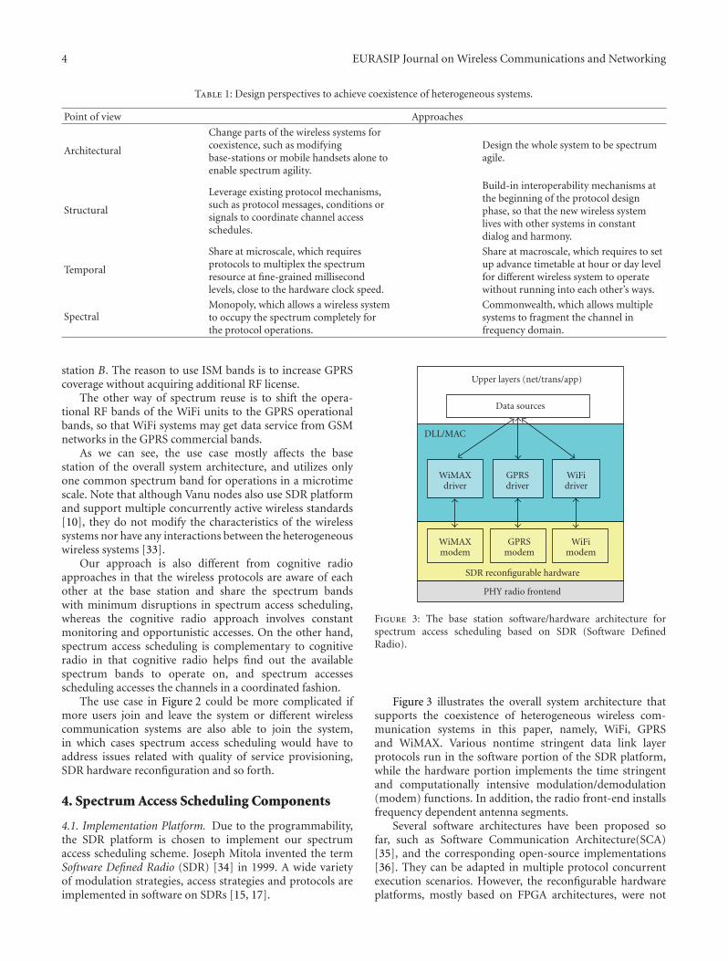
4 EURASIP Journal on Wireless Communications and Networking
Table 1: Design perspectives to achieve coexistence of heterogeneous systems.
Point of view Approaches
Architectural
Change parts of the wireless systems forcoexistence, such as modifyingbase-stations or mobile handsets alone toenable spectrum agility.
Design the whole system to be spectrumagile.
Structural
Leverage existing protocol mechanisms,such as protocol messages, conditions orsignals to coordinate channel accessschedules.
Build-in interoperability mechanisms atthe beginning of the protocol designphase, so that the new wireless systemlives with other systems in constantdialog and harmony.
Temporal
Share at microscale, which requiresprotocols to multiplex the spectrumresource at fine-grained millisecondlevels, close to the hardware clock speed.
Share at macroscale, which requires to setup advance timetable at hour or day levelfor different wireless system to operatewithout running into each other’s ways.
SpectralMonopoly, which allows a wireless systemto occupy the spectrum completely forthe protocol operations.
Commonwealth, which allows multiplesystems to fragment the channel infrequency domain.
station B. The reason to use ISM bands is to increase GPRScoverage without acquiring additional RF license.
The other way of spectrum reuse is to shift the opera-tional RF bands of the WiFi units to the GPRS operationalbands, so that WiFi systems may get data service from GSMnetworks in the GPRS commercial bands.
As we can see, the use case mostly affects the basestation of the overall system architecture, and utilizes onlyone common spectrum band for operations in a microtimescale. Note that although Vanu nodes also use SDR platformand support multiple concurrently active wireless standards[10], they do not modify the characteristics of the wirelesssystems nor have any interactions between the heterogeneouswireless systems [33].
Our approach is also different from cognitive radioapproaches in that the wireless protocols are aware of eachother at the base station and share the spectrum bandswith minimum disruptions in spectrum access scheduling,whereas the cognitive radio approach involves constantmonitoring and opportunistic accesses. On the other hand,spectrum access scheduling is complementary to cognitiveradio in that cognitive radio helps find out the availablespectrum bands to operate on, and spectrum accessesscheduling accesses the channels in a coordinated fashion.
The use case in Figure 2 could be more complicated ifmore users join and leave the system or different wirelesscommunication systems are also able to join the system,in which cases spectrum access scheduling would have toaddress issues related with quality of service provisioning,SDR hardware reconfiguration and so forth.
4. Spectrum Access Scheduling Components
4.1. Implementation Platform. Due to the programmability,the SDR platform is chosen to implement our spectrumaccess scheduling scheme. Joseph Mitola invented the termSoftware Defined Radio (SDR) [34] in 1999. A wide varietyof modulation strategies, access strategies and protocols areimplemented in software on SDRs [15, 17].
Upper layers (net/trans/app)
Data sources
DLL/MAC
WiMAXdriver
GPRSdriver
WiFidriver
WiMAXmodem
GPRSmodem
WiFimodem
SDR reconfigurable hardware
PHY radio frontend
Figure 3: The base station software/hardware architecture forspectrum access scheduling based on SDR (Software DefinedRadio).
Figure 3 illustrates the overall system architecture thatsupports the coexistence of heterogeneous wireless com-munication systems in this paper, namely, WiFi, GPRSand WiMAX. Various nontime stringent data link layerprotocols run in the software portion of the SDR platform,while the hardware portion implements the time stringentand computationally intensive modulation/demodulation(modem) functions. In addition, the radio front-end installsfrequency dependent antenna segments.
Several software architectures have been proposed sofar, such as Software Communication Architecture(SCA)[35], and the corresponding open-source implementations[36]. They can be adapted in multiple protocol concurrentexecution scenarios. However, the reconfigurable hardwareplatforms, mostly based on FPGA architectures, were not
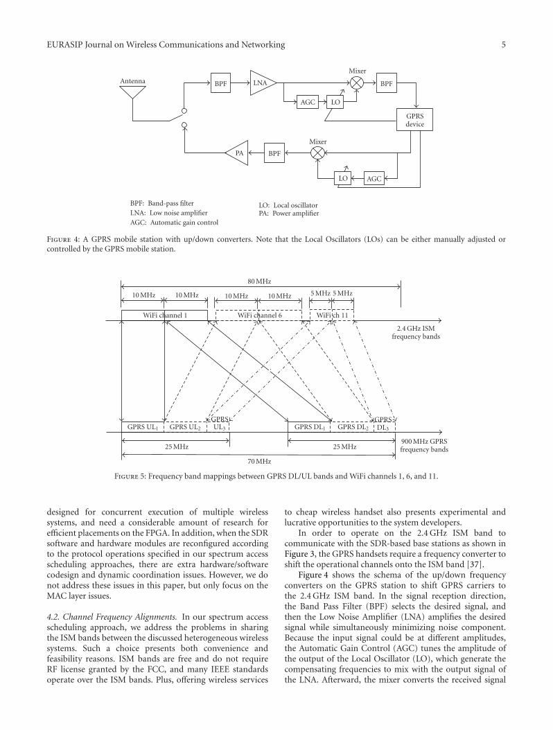
EURASIP Journal on Wireless Communications and Networking 5
Antenna LNABPF
AGC LO
BPF
Mixer
Mixer
PA BPF
LO AGC
GPRSdevice
BPF: Band-pass filterLNA: Low noise amplifierAGC: Automatic gain control
LO: Local oscillatorPA: Power amplifier
Figure 4: A GPRS mobile station with up/down converters. Note that the Local Oscillators (LOs) can be either manually adjusted orcontrolled by the GPRS mobile station.
WiFi channel 1 WiFi channel 6 WiFi ch 11
GPRS DL1 GPRS DL2
GPRSDL3
25 MHz25 MHz
GPRS UL1 GPRS UL2
GPRSUL3
900 MHz GPRSfrequency bands
2.4 GHz ISMfrequency bands
70 MHz
10 MHz 10 MHz 10 MHz 10 MHz 5 MHz 5 MHz
80 MHz
Figure 5: Frequency band mappings between GPRS DL/UL bands and WiFi channels 1, 6, and 11.
designed for concurrent execution of multiple wirelesssystems, and need a considerable amount of research forefficient placements on the FPGA. In addition, when the SDRsoftware and hardware modules are reconfigured accordingto the protocol operations specified in our spectrum accessscheduling approaches, there are extra hardware/softwarecodesign and dynamic coordination issues. However, we donot address these issues in this paper, but only focus on theMAC layer issues.
4.2. Channel Frequency Alignments. In our spectrum accessscheduling approach, we address the problems in sharingthe ISM bands between the discussed heterogeneous wirelesssystems. Such a choice presents both convenience andfeasibility reasons. ISM bands are free and do not requireRF license granted by the FCC, and many IEEE standardsoperate over the ISM bands. Plus, offering wireless services
to cheap wireless handset also presents experimental andlucrative opportunities to the system developers.
In order to operate on the 2.4 GHz ISM band tocommunicate with the SDR-based base stations as shown inFigure 3, the GPRS handsets require a frequency converter toshift the operational channels onto the ISM band [37].
Figure 4 shows the schema of the up/down frequencyconverters on the GPRS station to shift GPRS carriers tothe 2.4 GHz ISM band. In the signal reception direction,the Band Pass Filter (BPF) selects the desired signal, andthen the Low Noise Amplifier (LNA) amplifies the desiredsignal while simultaneously minimizing noise component.Because the input signal could be at different amplitudes,the Automatic Gain Control (AGC) tunes the amplitude ofthe output of the Local Oscillator (LO), which generate thecompensating frequencies to mix with the output signal ofthe LNA. Afterward, the mixer converts the received signal

6 EURASIP Journal on Wireless Communications and Networking
AGC
LNA
LNA
LNA
LO
Mixer
Mixer
BPFBPF
Antenna
BPF
BPF
BPF
BPF
BPFPA
PA
PA
BPF
BPF
GPRSdevice
LO
LO
LO
LO
LO
BPF : Band-pass filterLNA: Low noise amplifierLO: Local oscillator
AGC : Automatic gain controlPA: Power amplifier
AGC
AGC
AGC
AGC
AGC
Figure 6: The GPRS mobile station can utilize all the channels through three up/down converter pairs.
WiFi channel 1or
GPRS
WiFi channel 6or
GPRS
WiFi channel 6or
GPRS
WiFi channel 6or
GPRS
WiFi channel 6or
GPRS
WiFi channel 1or
GPRS
WiFi channel 1or
GPRS
WiFi channel 1or
GPRS
WiFi channel 1or
GPRS
WiFi channel 1or
GPRS
WiFi channel 11or
GPRS
WiFi channel 11or
GPRS
WiFi channel 11or
GPRS
WiFi channel 11or
GPRS
Figure 7: Channel planning of ISM channels in GPRS+WiFicoexistence network.
to the desired frequency band, and the desired signal isextracted by the BPF and sent into the cell phone.
The signal transmitting process is similar to the receivingprocess in the reverse direction.
Essentially, the formula of the converter in Figure 4 is
fchann = foper + fLO (1)
in which fchann is the channel frequency that goes into andfrom the antenna, foper is the operating frequency of theGPRS device, and fLO is the add-on frequency generated bythe local oscillators.
The local oscillators would know which frequencythat the GPRS mobile station is going to transmit or toreceive signals. There are two mechanisms to acquire suchknowledge—one is to fix on the channel frequency manually,and the other is to allow the frequency converter dynamicallyto choose the channel frequency depending on the spectrumavailability. The second approach is what the cognitiveradio research focused on and is where spectrum accessscheduling can take advantage of the results and mechanismsof cognitive radio. In this paper, we limit our discussionsto the first approach in which the channel frequencies arelocated in the ISM bands.
However, WiFi 2.4 GHz operating band is about 80 MHzwith three noneoverlapping WiFi channels in the US, whilethe total operating frequency band of GPRS is around70 MHz, including the 45 MHz downlink/uplink (DL/UL)separation and the DL/UL bandwidth 25 MHz each. There-fore, if GPRS operating channels are plainly converted intothe 2.4 GHz ISM bands, GPRS will impact every nonover-lapping WiFi channel, which is inefficient and difficult tocoordinate.
We solve this problem by modifying the add-on fre-quency of the local oscillator in the frequency up/down

EURASIP Journal on Wireless Communications and Networking 7
SIFSCTS
SIFSACK
Defer access
NAV (CTS)NAV (RTS)
Time
Time
Time
DataSIFS
RTS
Backoff
DIFSSender
Receiver
BusyOtherstations
Figure 8: IEEE 802.11 DCF channel access coordination withRTS/CTS and NAV mechanisms.
converter, as given in Figure 4. That is, we fit the GPRSDL/UL bands into the 20 MHz WiFi/WiMAX channels byshifting different frequency offsets, respectively, and offeringnarrower DL/UL bandwidths. This way, both GPRS DL/ULbands can be mapped to different portions of a WiFi channel.
Figure 5 illustrates the ways that the WiFi channels aremapped to the GSM/GPRS frequency bands. We can eitherutilize only one of the three channels 1, 6 and 11 to composeparts of the DL/UL frequency bands in GPRS, as shownby the solid lines and boxes or utilize all the 2.4 GHz WiFibands so as to patch up the complete GPRS frequencyspectrum at the 900 MHz frequency ranges. Note that not allof WiFi channel 11 was utilized to carry GPRS bands, and themapping from GPRS spectrum to the WiFi spectrum couldbe even made such that each WiFi channel carries the sameproportion of the GPRS spectrum.
Certainly, utilizing just one of the WiFi channels is easierto manage than more WiFi channels because the base stationonly has to coordinate wireless stations operating in onechannel, and the implementation is the same as shown inFigure 4. However, if the base station’s operating channelis not fixed to a certain WiFi channel, the mobile stationwould have to control the local oscillators in the up/downconverter to shift GPRS signals to and from the properWiFi channels. As shown in Figure 4, an interface in theGPRS device is provided to connect and control the localoscillators.
On the other hand, utilizing the whole WiFi spectrumto compose the complete GPRS spectrum is not difficultto achieve. Figure 6 shows the implementation that usesthree pairs of frequency up/down converters on the mobileGPRS handset in order to achieve the full GPRS operatingspectrum.
4.3. Cellular Architecture. Similar to the GSM/GPRS cellulararchitecture, we can build cellular networks using spec-trum access scheduling base stations using the ISM bands.According to the frequency mapping in Figure 5, a three-cellclustering structure can be adopted as shown in Figure 7.As we can see, cells within a cluster use disjointed set offrequencies so as to avoid channel collisions, and cells thatuse the same frequency channel are separated by one celldistance, as shown by gray areas in Figure 7.
In order to avoid intercell interferences, the base stationof each cell needs to apply power control mechanisms to both
0.577 ms4.615 ms
GSM TDMA frame
1 2 3 4 5 6 7 8
Frequency(MHz)
Time
960
Downlink
935
915
Uplink
890
200 KHz
Figure 9: The GSM system includes the downlink/uplink bands.Each GSM frame consists of 8 time slots (bursts).
GPRS stations and WiFi/WiMAX stations. Because we havearranged the ISM band operators, WiFi and WiMAX, as thehosting wireless systems, GPRS, which is a Wireless WideArea Network (WWAN) technology, will apply the powercontrol mechanisms to obey the FCC regulations for usingthe ISM band. This further helps optimize the talk time andstandby time of the GPRS handsets.
5. Channel Access Control and Evaluations
The essential mechanisms to coordinate distributed channelaccess control follow two channel access schemes; (1)random channel access scheme, such as CSMA, CSMA/CA,and pure and slotted ALOHA, which were most extensivelyused and studied, for example, MACA, MACAW [38], IEEE802.11 DCF [39], PAMAS [40]; and (2) scheduled channelaccess scheme, such as FDMA, TDMA, CDMA mechanismsin wireless cellular networks, GSM, UMTS and CDMA2000systems [41].
WiFi standard IEEE 802.11 [42] has adopted the ran-domized channel access scheme using the CSMA/CA mecha-nisms. The other two wireless systems, GPRS and WiMAX,are based on the scheduled channel access control schemeusing the TDMA scheme.
The difficulty of achieving the coexistence of any twowireless systems lies in the fact that we can only modifylimited number architectural components, such as the basestations in our spectrum access scheduling approach. There-fore, without proper control over the protocol operations,the unmodified system components of one wireless systemmay unexpectedly interrupt the ongoing packet receptionin another wireless system, causing collisions. Such possiblescenario happens especially when one of the coexistingwireless system operates using the random access scheme.
Therefore, we discuss two coexistence scenarios, namely,GPRS+WiFi and GPRS+WiMAX, respectively, for spectrumaccess scheduling purposes in the TDMA fashion. TheGPRS+WiFi scenario integrates the scheduled and ran-dom access schemes, whereas the GPRS+WiMAX scenarioinvolves different wireless systems under only the scheduled

8 EURASIP Journal on Wireless Communications and Networking
T T T T T T T TN0
PB
PA
PC
PA
PA
PA
PA
PA
PA
PD P
DPD
PD
PD
PD
PD P
BPA
PC
PA
PA
PA
PA
PA
PA
PD P
DPD
PD
PD
PD
PD P
BPA
PC
PA
PA
PA
PA
PA
PA
PD P
DPD
PD
PD
PD
PD P
BPA
PC
PA
PA
PA
PA
PA
PA
PD P
DPD
PD
PD
PD
PD
1 2 3 4 5 6 7N N N N N N N
T T T T T T T TN0 1
RLC/MAC block
2 3 4 5 6 7N N N N N N N
T T T T T T T TN0 1 2 3 4 5 6 7
N N N N N N NT T T T T T T TN0 1 2 3 4 5 6 7
N N N N N N N
PC: Packet common control channelTN: Time slot
PB: Packet BCCHPD: Packet data channelPA: Packet associated control channel
Figure 10: Possible configuration of a GPRS downlink radio channel.
TDD frame n− 1 TDD frame n TDD frame n + 1
DL subframe TTG UL subframe RTG TDD downlink/uplinkarrangement
Downlink burststructurePreamble FCH DL burst #1 DL burst #2 DL burst #n· · ·
DLFP MAC PDU1 · · · MAC PDUn Pad
DL-MAP UL-MAP DCD UCD MAC PDUsDownlink structure
descriptors
Broadcast to all SSs
Figure 11: Fixed WiMAX/TDD frame structure and burst information.
channel access scheme. Specifically, we present the necessarychanges to the protocol messaging at the base stations inorder to prevent the unmodified wireless stations fromstepping into each other for channel access.
In this section, we first briefly provide a tutorial aboutthe channel access control mechanisms in WiFi, GPRS andWiMAX, then specify the protocol control mechanisms toenable the coexistence of heterogeneous wireless systems.
5.1. Background Review.
5.1.1. IEEE 802.11b (WiFi). The channel access methodin IEEE 802.11 Distributed Coordination Function (DCF)is based on Carrier Sensing Multiple Access (CSMA) forsharing a common channel [42]. It is essentially a time-division multiplexing method, only that the time slots arevirtual and flexible to the transmission time of each dataframe.
DCF use five basic mechanisms to inform and resolvechannel access conflicts:
(1) carrier sensing (CS) before each transmission,
(2) collision avoidance using RTS/CTS control messages,
(3) interframe spacings (IFSs) to prioritize differenttypes of messages,
(4) binary exponential backoff (BEB) mechanism torandomize among multiple channel access attempts,
(5) network Allocation Vector (NAV) for channel reser-vation purposes.
Figure 8 illustrates the CSMA/CA access method withNAV. Using the RTS and CTS frames, which carry the NAVinformation, the sender and the receiver can reserve theshared channel for the duration of the data transmissions,thus avoiding possible collisions from other overhearingstations in the network.
The NAV-based channel reservation mechanism will beutilized in spectrum access scheduling for allocating timeperiods for heterogeneous wireless system operations.
5.1.2. GPRS (General Packet Radio Service). GPRS is anenhancement over the existing GSM systems by using thesame air interface and channel access control procedure.Specifically, we discuss the GPRS systems based on the GSM-900 bands. In GSM-900, the downlink (DL) and uplink (UL)frequency bands are 25 MHz wide each and each band isdivided into 200 KHz channels. The frequency separationbetween the corresponding downlink and uplink channels is45 MHz.

EURASIP Journal on Wireless Communications and Networking 9
TTG RTG RTG
One frame = 8 GPRStime slots = 4.615 ms
Time
GPRS UL
GPRS DL
GPRS UL
GPRS DLULsubframe
DLsubframe
DLsubframe
ULsubframe
TTG
Frequency
2.4 GHz20
MH
z
Figure 12: GPRS and WiMAX time sharing the ISM band.
T TTT T T TTN0 1 2 3 4 5 6 7
NNNNNNNT TTTT T TTN0 1 2 3 4 5 6 7
NNNNNNNT TT T T T TTN0 1 2 3 4 5 6 7
NNNNNNNT TTT T T TTN0 1 2 3 4 5 6 7
NNNNNNNT TTT
Frame 8
Time
Time
WiMAXWiMAXWiMAXWiMAXWiMAXWiMAXDownlink
UplinkWiMAXWiMAXWiMAXWiMAXWiMAXWiMAX
Frame 7Frame 6Frame 5Frame 4Frame 3
Frame 8Frame 7Frame 6Frame 5
Block
Frame 4Frame 3
T T TTN0 1 2 3 4 5 6 7
NNNNNNNT TTT T T TTN0 1 2 3 4 5 6 7
NNNNNNN
T TTT T T TTN5 6 7 0 1 2 3 4
NNNNNNNT TTTT T TTN5 6 7 0 1 2 3 4
NNNNNNNT TT T T T TTN5 6 7 0 1 2 3 4
NNNNNNNT TTT T T TTN5 6 7 0 1 2 3 4
NNNNNNNT TTT T T TTN5 6 7 0 1 2 3 4
NNNNNNNT TTT T T TTN5 6 7 0 1 2 3 4
NNNNNNN
Figure 13: The allocation of uplink and downlink time slots.
Base station
GGSNSGSNHost 1
GPRS station
Host 2
WiMAX subscriberstation
Figure 14: The topology of the simulated GPRS+WiMAX coexis-tence network.
Figure 9 shows a GSM-900 TDMA frame and its slots.The duration of a frame is 4.615 milliseconds with 8 timeslots, each of which lasts for 0.557 milliseconds [43] .
The GPRS downlink and uplink channels are centrallycontrolled and managed by the base stations (BSs). GPRSuses the same physical channels as in GSM, but organizesthem differently from GSM. In GPRS, the Data Link Layer(DLL) data-frame is mapped to a radio block, which isdefined as an information block transmitted over a physicalchannel of four consecutive frames [43].
With regard to the GPRS channel access mechanisms, wefirst look at the normal GPRS downlink channel operations,as shown in Figure 10.
In Figure 10, “TN” means the time slot number in each8-slot time frame. Each time slot could be dedicated for thefollowing purposes.
(i) A single purpose. For example, “TN0” marked with“PB” are used as the PBCCH (Packet Broadcast ControlCHannel) logical channel to beacon the GPRS packet systeminformation at the position of block 0 of a 52-frame multi-frame.
(ii) Multiple purposes. For example, “TN1” markedwith “PD/PA/PC” is used as PDTCH (Packet Data TrafficCHannel) to transfer data traffic or as PACCH (PacketAssociated Control CHannel) to be associated with a GPRStraffic channel to allocate bandwidth or as PCCCH (PacketCommon Control CHannel) for request/reply messagesto access the GPRS services. The PCCCH includes threesubchannels, Packet Random Access CHannel (PRACH),Packet Access Grant CHannel (PAGCH), and Packet PagingChannel (PPCH) [43].
GPRS stations use the PRACH to initiate a packettransfer by sending their requests for access to the GPRSnetwork service, and listen to the PAGCH for a packet uplinkassignment. The uplink assignment message includes the listof PDCH (Packet Data CHannels) and the corresponding

10 EURASIP Journal on Wireless Communications and Networking
0 2 4 6 8 10 12 14
Load (Kbps)
12345678
Th
rou
ghpu
t(K
bps)
(a) GPRS Throughput
0 2 4 6 8 10 12 14
Load (Mbps)
123456789
10
Th
rou
ghpu
t(M
bps)
(b) WiMAX Throughput
0 2 4 6 8 10 12 14 16
Load (Kbps)
0.60.8
11.21.41.61.8
22.22.42.6
En
d-to
-en
dde
lay
(s)
(c) GPRS End-to-End Delay
0 2 4 6 8 10 12 14
Load (Mbps)
012345678
En
d-to
-en
dde
lay
(s)
(d) WiMAX End-to-End Delay
0 2 4 6 8 10 12 14
Load (Kbps)
0
2
4
6
8
10
12×102
Nu
mbe
rof
drop
pack
ets
(e) GPRS Packet Loss
0 2 4 6 8 10 12 14
Load (Mbps)
012
3
45
67×104
Nu
mbe
rof
drop
pack
ets
(f) WiMAX Packet Loss
Figure 15: Network performance in GPRS+WiMAX coexisting systems.
One frame = 8 GPRStime slots = 4.615 ms
NAV1NAV2
NAV3
Time
GPRS UL
GPRS DL Channelbusy GPRS UL
GPRS DLChannelbusy R
TS
RT
S
RT
S
Frequency
2.4 GHz
20M
Hz
Figure 16: GPRS and WiFi time sharing the ISM band.
Uplink Status Flag (USF) values per PDCH. GPRS stationskeep listening to the USFs of the allocated PDCHs. If thecorresponding USF is set, it means that the GPRS station hasnow been granted access to the next PDCH block.
Not all the GPRS stations have the capability to simul-taneously transmit and receive. Half-duplex mobile stationscan communicate in only one direction at a time. In afull-duplex system, stations allow communication in bothdirections simultaneously.
5.1.3. IEEE 802.16-2004 (WiMAX). In this paper, we focuson the following IEEE 802.16-2004 (fixed WiMAX) systemfor spectrum access scheduling: (a) a single cell operatingin the Point-to-MultiPoint (PMP) mode, (b) no mobility,
(c) use of 2.4 GHz unlicensed bands, and (d) use of TimeDivision Duplex (TDD) as the channel duplexing scheme.
Figure 11 illustrates a WiMAX frame structure usingthe TDD scheme [44]. A frame consists of a downlink(DL) subframe and an uplink (UL) subframe, interleavedby two transition gaps, the RTG (receive/transmit transi-tion gap) and TTG (transmit/receive transition gap). Bothgap durations are adjustable according to user’s needs.A downlink subframe starts with a long preamble forsynchronization purposes. A Frame Control Header (FCH)burst follows the preamble, and contains the DownlinkFrame Prefix (DLFP), which specifies the downlink burstprofile. In the first downlink burst, optional DL-MAP andUL-MAP indicate the starting time slot of each following

EURASIP Journal on Wireless Communications and Networking 11
Base station 1
Base station 3
WiFi channel 11
WiFi channel 1
WiFi channel 6
Base station 2
GPRS mobile station
IEEE 802.11bmobile station
Figure 17: The network topology with three base stations in themobile scenario.
MAC PDU data burst in downlink and uplink transmis-sions, respectively. The additional information contained inDownlink Channel Descriptor (DCD) and Uplink ChannelDescriptor (UCD) tells the physical layer characteristics ofthe downlink and uplink channels, such as the modulationalgorithm, forward error-correction type, and the preamblelength.
5.2. Coexistence of GPRS and WiMAX.
5.2.1. Specifications. In the time domain, GPRS and WiMAXbased on WiMAX share the frequency bands in a roundrobin fashion, and the granularity of the channels is theGSM time frame, which is at the level of milliseconds. Toavoid confusions, we use WiMAX to specifically mean IEEE802.16-2004 in the following discussions if not indicatedotherwise.
As we know, the duration of a GPRS frame is4.615 milliseconds. Although the default frame durationsin IEEE 802.16-2004 does not include 4.615 milliseconds,WiMAX frame does have different frame durations tobe chosen and have adjustable periods for time framealignments, such as the RTG and the TTG.
Figure 12 shows the time-sharing scheme between GPRSand WiMAX during the period of two time frames. In thisscenario, WiMAX is the hosting system, which uses twoadjustable gaps, RTG and TTG between downlink and uplinksubframes, to control the amount of time left for GPRS. Weset the RTG time to around 3 GPRS time slots. When theWiMAX channel is around 20 MHz, it provides the GPRSsystems with about (10 MHz/200 KHz) × 3 = 150 physicalchannels in each of downlink and uplink directions.
In addition, the portions allocated to WiMAX and GPRScan be flexible. We discuss only the fixed allocations toeach of the wireless systems for simplicity, and leave traffic-dependent dynamic allocation scheme as future research.
In our channel allocation scheme as shown in Figure 12,only three of the eight time slots can be used. Figure 13 shows
an example how GPRS systems operate with only three timeslots per frame. The shaded time slots illustrate the downlinkand uplink time slots used by a specific mobile station only.
Note that in GPRS networks, the uplink and downlinktime slot numbers are separated by three time slots, as shownin Figure 13. Hence, if we use the first three downlink timeslots in the GPRS period in Figure 12, the uplink time slotscan only be “TN5-7”. Although not having the “TN0” inuplink seemed like a problem, such a scheme actually worksas shown by the shaded time slots. In such arrangements,the downlink GPRS block and the uplink GPRS block areseparated by five time slots, long enough for a half-duplexGPRS to get ready to receive and transmit sequentially.
5.2.2. Performance Evaluations. We use the network simula-tor NCTUns 4.0 [45] to simulate the coexistence of the twowireless systems GPRS and WiMAX. The NCTUns simulatorprovides the implementations of GPRS and WiMAX withenough details in the physical and data link layers toallow us to realize spectrum access scheduling mechanisms.Specifically, we modify the base station modules in orderto control the channel access mechanisms, and enable thecoexistence of heterogeneous systems in the same spectrumbands. One simple static scenario is simulated in which asingle base station supports one stationary GPRS handsetand one WiMAX stationary subscriber hosts.
Figure 14 illustrates the network configuration for testingthe coexistence of GPRS and WiMAX in the same spectrumbands. On the infrastructure side, one SGSN (Serving GPRSSupport Node) and one GGSN (Gateway GPRS SupportNode) were placed behind the base station to transfer GPRSrelated data packets. GGSN is the Internet gateway routerthat is responsible for sending data packets to the InternetHose 1 in Figure 14. In this scenario, we do not considermobility.
We use CBR traffic in various data rates to evaluatethe throughput, delay and packet loss characteristics of thetraffic for GPRS and WiMAX systems, respectively. Two CBRconnections are simulated in each traffic load configuration,namely, the connections starts from the WiMAX SubscriberStation to the fixed Host 2, and from the GPRS Station to thefixed Host 1, respectively.
The GPRS CBR data packet has a payload size of 100bytes, and the WiMAX CBR data packet payload is of size1000 bytes. The effective network loads are from 1 to 15 Kbpsfor the GPRS system, and from 1 to 15 Mbps for the WiMAXsystem. The raw data rate of the WiMAX system is 54 Mbps.
Figure 15 shows the network throughput, end-to-enddelay and packet losses of the GPRS and WiMAX connec-tions side by side. Because of the dramatic differences, GPRSand WiMAX system performance is shown in two columns,respectively. As shown in Figure 15, increasing the networkload affects the throughput, end-to-end delays and packetlosses. The network throughput saturates when the trafficloads go beyond certain points in both GPRS and WiMAX,at which the network delays and packet losses also startincreasing dramatically. The key observation that we learnfrom the experiments is that both GPRS and WiMAX systems

12 EURASIP Journal on Wireless Communications and Networking
0 2 4 6 8 10 12 14
Load (Kbps)
12345678
Th
rou
ghpu
t(K
bps)
(a) GPRS Throughput
0 0.2 0.4 0.6 0.8 1 1.2 1.4
Load (Mbps)
00.10.20.30.40.50.60.70.80.9
Th
rou
ghpu
t(M
bps)
(b) WiFi Throughput
0 2 4 6 8 10 12 14
Load (Kbps)
0.60.8
11.21.41.61.8
22.22.42.6
En
d-to
-en
dde
lay
(s)
(c) GPRS End-to-End Delay
0 0.2 0.4 0.6 0.8 1 1.2 1.4
Load (Mbps)
0.20.220.240.260.28
0.30.320.340.360.38
En
d-to
-en
dde
lay
(s)
(d) WiFi End-to-End Delay
0 2 4 6 8 10 12 14
Load (Kbps)
0
2
4
6
8
10
12×102
Nu
mbe
rof
drop
pack
ets
(e) GPRS Packet Loss
0 0.2 0.4 0.6 0.8 1 1.2 1.4
Load (Mbps)
0102030405060708090×102
Nu
mbe
rof
drop
pack
ets
(f) WiFi Packet Loss
Figure 18: GPRS and WiFi network performance in coexistence (mobility).
operate normally under the coexistence situations due tothe careful planning of channel access control in the timedomain.
5.3. Coexistence of GPRS and WiFi.
5.3.1. Specifications. WiFi systems based on IEEE 802.11DCF are totally different from WiMAX channel accessschemes in that channel access is randomized, and networkservices are provided on the best-effort basis.
Different from achieving the coexistence of GPRS andWiMAX systems, we adapt the RTS control frames toallocation channel time periods for GPRS operations, as usedby the Bluetooth and WiFi coexistence proposal [2].
Figure 16 illustrates the way of GPRS and WiFi sharingthe 20 MHz wide 2.4 GHz ISM band. In this applicationscenario, WiFi is the hosting system. As we know, the NAVvalue in IEEE 802.11 is a 16-bit integer attached in eachpacket, indicating the duration of the immediate followingdata exchange period in the unit of microseconds. Therefore,the NAV can represent a duration up to 64 milliseconds,enough to reserve the channel for GPRS. In order to reservethe channel for GPRS systems, the base station of the WiFi
system sends an RTS control frame to itself, and sets the NAVvalue long enough for the GPRS to operate.
The duration of NAV is set such that the reserved periodcan cover 3 GPRS time slot period, and that the end of theNAV channel reservation is the beginning of the next WiFichannel access.
Similar to the coexistence arrangement of GPRS andWiMAX channel access, the portions allocated to WiMAXand GPRS can be flexible. We discuss only the fixedallocations to each of the wireless systems for simplicity, andleave traffic-dependent dynamic allocation scheme as futurework.
The timing of special channel-reservation RTS transmis-sions is calculated and controlled by the base station. Whenthe channel data rate and the regular duration of a dataframe transmission is known beforehand, the base stationcan estimate the possibility of the channel being occupiedby the mobile stations or the base station itself when theGPRS due time arrives. If the channel will be potentiallyoccupied by stations in the cell, the base station will preemptthe channel with the RTS-to-itself control message so as toprevent WiFi packet transmission extending into the GPRSperiods. The time before GPRS periods when WiFi stations

EURASIP Journal on Wireless Communications and Networking 13
should stop access the channel is called “danger zone”. Oncethe time advances into the “danger zone”, the base stationshall grab the channel in the first moment when the channelbecomes idle by sending the special RTS control message.
If the “danger zone” is long enough, the base stationcould choose to send multiple RTS messages to ensure thechannel reservation message RTS is received by all the mobilestations in the cell, as shown by the second GPRS time frameperiod in Figure 16.
When the base station enters the GPRS operationalperiod, it carries out the GPRS data communication func-tionalities. Once the NAV expires, mobile stations and thebase station can enter the IEEE 802.11 DCF mode to contendfor channel accesses.
5.3.2. Performance Evaluations. We again use the NCTUnssimulator for evaluating the performance of GPRS+WiFicoexistence systems. In the simulations, we use the sametopology, packet sizes and network loads as GPRS+WiMAXsimulations in Figure 14, except that the WiMAX SubscriberStation is changed to a WiFi station.
Different from the GPRS+WiMAX simulation scenario,a mobile setting is simulated in GPRS+WiFi coexistencescenario to test the feasibility of handling mobility inGPRS+WiFi coexistence networks. As shown by Figure 17,three base stations are deployed in the field, each operatingon a different frequency channel as shown in Figure 7, andtwo GPRS and WiFi mobile stations move across the fieldalong the dotted lines while carrying out data transmissions.For simplicity, we have omitted the infrastructure nodesSGSN, GGSN and the fixed hosts. The CBR traffic assign-ments and load increment schedule are the same as theprevious simulations.
Figure 18 shows the network performance of theGPRS+WiFi coexistence network in terms of the CBR trafficthroughput, the packet end-to-end delay and the packet loss.If we compare the performance of GPRS in both Figures 15and 18, it shows that the fixed GPRS station achieved a littlebit better performance than that in mobile situations. This isdue to the handover operations, in which packet loss couldhappen. However, other than that, GPRS traffic performanceis approximately the same due to similar channel accessschedules in both coexistence scenarios. On the other hand,WiFi achieves maximum throughput at 0.9 Mbps, much lessthan WiMAX in the previous coexistence systems. This is dueto the lower data rate 11 Mbps in IEEE 802.11b, and thehigher control overhead using the RTS control frames.
6. Conclusion
We have presented a new spectrum sharing scheme, calledspectrum access scheduling, to improve the spectrum effi-ciency in the temporal domain by allowing heterogeneouswireless networks to time-share the spectrum. Differentfrom cognitive radio approaches, which are opportunisticand noncollaborative in general, spectrum access schedulingtreats the collection of select wireless systems as equal spec-trum share holders, and optimizes the system performanceby collaborative designs. We have looked at the spectrum
access scheduling design challenges from different perspec-tives, and proposed a time shared channel access paradigm bymodifying the wireless base stations using the SDR platform.Two heterogeneous wireless systems coexistence scenarios,GPRS+WiMAX and GPRS+WiFi, have been studied andsimulated. The performance results of the simulations showthat spectrum access scheduling is a feasible solution tothe spectrum sharing problem, and is worthy of furtherresearch.
Acknowlegment
This work was supported in part by the National ScienceFoundation (NSF) under Grant no. 0725914.
References
[1] FCC, “Spectrum Policy Task Force Report, ET Docket No. 02-155,” November 2002.
[2] C. F. Chiasserini and R. R. Rao, “Coexistence mechanismsfor interference mitigation between IEEE 802.11 WLANs andBluetooth,” in Proceedings of the 21st Annual Joint Conferenceof the IEEE Computer and Communications Societies (INFO-COM ’02), vol. 2, pp. 590–598, New York, NY, USA, June 2002.
[3] J. Kurose and K. Ross, Computer Networking: A Top-DownApproach Featuring the Internet, Addison Wesley, New York,NY, USA, 2005.
[4] V. Chandrasekhar, J. G. Andrews, and A. Gatherer, “Femtocellnetworks: a survey,” IEEE Communications Magazine, vol. 46,no. 9, pp. 59–67, 2008.
[5] S.-P. Yeh, S. Talwar, S.-C. Lee, and H. Kim, “WiMAXfemtocells: a perspective on network architecture, capacity,and coverage,” IEEE Communications Magazine, vol. 46, no.10, pp. 58–65, 2008.
[6] Sprint Inc., http://www.nextel.com/en/services/airave/index.shtml?id9=vanity:airave.
[7] Verizon Inc., http://www22.verizon.com.[8] “Femtocell,” October 2007, http://www.femtoforum.org/
femto/Files/File/Airvana%20Femtocell%20White%20Paper%20Oct%202007.pdf.
[9] “Ericsson’s Femto Cell Solution,” http://www.ericsson.com.[10] Vanu Inc., http://www.vanu.com.[11] H. Harada, “A study on a new wireless communications system
based on cognitive radio technology,” Tech. Rep. SR2005-17,IEICE, Tokyo, Japan, 2005.
[12] I. F. Akyildiz, W.-Y. Lee, M. C. Vuran, and S. Mohanty,“A survey on spectrum management in cognitive radionetworks,” IEEE Communications Magazine, vol. 46, no. 4, pp.40–48, 2008.
[13] I. F. Akyildiz, W.-Y. Lee, M. C. Vuran, and S. Mohanty, “Nextgeneration/dynamic spectrum access/cognitive radio wirelessnetworks: a survey,” Computer Networks, vol. 50, no. 13, pp.2127–2159, 2006.
[14] J. Mitola III, “Cognitive radio for flexible mobile multimediacommunications,” in IEEE International Workshop on InMobile Multimedia Communications (MOMUC ’99), pp. 3–10,1999.
[15] J. Mitola III, Software Radios: Wireless Architecture for the 21stCentury, John Wiley & Sons, New York, NY, USA, 1999.
[16] J. Mitola III, Cognitive radio: an integrated agent architecturefor software defined radio, Ph.D. thesis, Royal Institute ofTechnology, Stockholm, Sweden, 2000.

14 EURASIP Journal on Wireless Communications and Networking
[17] J. Mitola III and G. Q. Maguire Jr., “Cognitive radio: makingsoftware radios more personal,” IEEE Personal Communica-tions, vol. 6, no. 4, pp. 13–18, 1999.
[18] P. Kolodzy, et al., “Next generation communications: Kickoffmeeting,” in Proceedings of the Defense Advanced ResearchProjects Agency (DARPA ’01), October 2001.
[19] A. Sahai, N. Hoven, and R. Tandra, “Some fundamental limitson cognitive radio,” in Proceedings of Allerton Conference,Monticello, Minn, USA, October 2004.
[20] T. A. Weiss and F. K. Jondral, “Spectrum pooling: an innova-tive strategy for the enhancement of spectrum efficiency,” IEEECommunications Magazine, vol. 42, no. 3, pp. S8–S14, 2004.
[21] T. A. Weiss, J. Hillenbrand, A. Krohn, and F. K. Jondral,“Efficient signaling of spectral resources in spectrum poolingsystems,” in Proceedings of the 10th Symposium on Communica-tions and Vehicular Technology (SCVT ’03), Benelux, Novenber2003.
[22] R. W. Brodersen, A. Wolisz, D. Cabric, S. M. Mishra, and D.Willkomm, “Corvus: a cognitive radio approach for usage ofvirtual unlicensed spectrum,” Tech. Rep., Berkeley WirelessResearch Center (BWRC), Berkeley, Clif, USA, 2004.
[23] D. Cabric, S. M. Mishra, D. Willkomm, R. Brodersen, andA. Wolisz, “A cognitive radio approach for usage of virtualunlicensed spectrum,” in Proceeding of the 14th IST Mobile andWireless Communications Summit, Dresden, Germany, June2005.
[24] IEEE Working Group on Wireless Regional Area Networks(WRANs), “IEEE 802 LAN/MAN standards committee 802.22WG on WRANs,” Tech. Rep., IEEE, New York, NY, USA, April2008, http://www.ieee802.org/22.
[25] P. J. Jeong and M. Yoo, “Resource-aware rendezvous algorithmfor cognitive radio networks,” in Proceedings of the 9th Inter-national Conference on Advanced Communication Technology(ICACT ’07), vol. 3, pp. 1673–1678, Gangwon-do, SouthKorea, February 2007.
[26] FCC. ET Docket No. 03-108, “Facilitating Opportunities forFlexible and Efficient and Reliable Spectrum Use EmployingCognitive Radio Technologies,” March 2005.
[27] O. Holland, A. Attar, N. Olaziregi, N. Sattari, and A. H. Agh-vami, “A universal resource awareness channel for cognitiveradio,” in Proceedings of IEEE International Symposium onPersonal, Indoor and Mobile Radio Communications (PIMRC’06), pp. 1–5, Helsinki, Finland, September 2006.
[28] S. Krishnamurthy, M. Thoppian, S. Venkatesan, and R.Prakash, “Control channel based MAC-layer configuration,routing and situation awareness for cognitive radio networks,”in Proceedings of IEEE Military Communications Conference(MILCOM ’05), vol. 1, pp. 455–460, Atlantic City, NJ, USA,October 2005.
[29] L. Ma, X. Han, and C.-C. Shen, “Dynamic open spectrumsharing MAC protocol for wireless ad hoc networks,” inProceedings of the 1st IEEE International Symposium on NewFrontiers in Dynamic Spectrum Access Networks (DySPAN ’05),pp. 203–213, Baltimore, Md, USA, November 2005.
[30] M. M. Buddhikot, P. Kolody, S. Miller, K. Ryan, and J. Evans,“DIMSUMNet: new directions in wireless networking usingcoordinated dynamic spectrum access,” in Proceedings of the6th IEEE International Symposium on a World of WirelessMobile and Multimedia Networks (WoWMoM ’05), pp. 78–85,Taormina, Italy, June 2005.
[31] D. Raychaudhuri and X. Jing, “A spectrum etiquette protocolfor efficient coordination of radio devices in unlicensedbands,” in Proceedings of the 14th IEEE Personal, Indoor and
Mobile Radio Communications (PIMRC ’03), vol. 1, pp. 172–176, Beijing, China, September 2003.
[32] A. C.-C. Hsu, D. S. L. Wei, and C.-C. J. Kuo, “A cognitiveMAC protocol using statistical channel allocation for wirelessad-hoc networks,” in Proceedings of IEEE Wireless Communi-cations and Networking Conference (WCNC ’07), pp. 105–110,Kowloon, Hong Kong, March 2007.
[33] F. K. Jondral, “Software-defined radio—basics and evolutionto cognitive radio,” EURASIP Journal on Wireless Communica-tions and Networking, vol. 2005, no. 3, pp. 275–283, 2005.
[34] J. Mitola III, “Software radio architecture: a mathematical per-spective,” IEEE Journal on Selected Areas in Communications,vol. 17, no. 4, pp. 514–538, 1999.
[35] JTRS, http://sca.jpeojtrs.mil/.[36] CRC, SCARI-OPEN http://www.crc.ca.[37] S. Haykin, Communication Systems, John Wiely & Sons, New
York, NY, USA, 4th edition, 2001.[38] V. Bharghavan, A. Demers, S. Shenker, and L. Zhang,
“MACAW: a media access protocol for wireless LANs,”in Proceedings of the ACM Conference on CommunicationsArchitectures, Protocols and Applications (SIGCOMM ’94), pp.212–225, London, UK, August 1994.
[39] IEEE Std 802.11, “Wireless lAN medium access control (MAC)and physical layer (PHY) specifications,” Tech. Rep., IEEE,New York, NY, USA, July 1997.
[40] S. Singh and C. S. Raghavendra, “PAMAS: power aware multi-access protocol with signalling for ad hoc networks,” ComputerCommunication Review, vol. 28, no. 3, pp. 5–25, 1998.
[41] J. Schiller, Mobile Communication, Addison Wesley, New York,NY, USA, 2nd edition, 2003.
[42] IEEE Std 802.11, “Part 11: wireless lAN medium access control(MAC) and physical layer (PHY) specifications,” Tech. Rep.,IEEE, New York, NY, USA, 2007.
[43] P. McGuiggan, GPRS in Practice: A Companion to the Specifi-cation, John Willey & Sons, New York, NY, USA, 2004.
[44] IEEE Std 802.16-2004, “IEEE standard for local andmetropolitan area networks—part 16: air interface for FixedBroadband Wireless Access Systems,” Tech. Rep., IEEE, NewYork, NY, USA, October 2004.
[45] “NCTUns 4.0 Network Simulator and Emulator,”http://nsl.csie.nctu.edu.tw/nctuns.html.

Hindawi Publishing CorporationEURASIP Journal on Wireless Communications and NetworkingVolume 2010, Article ID 142921, 7 pagesdoi:10.1155/2010/142921
Research Article
Efficient Scheduling of Pigeons for a Constrained DelayTolerant Application
Jiazhen Zhou, Jiang Li, and Legand Burge
Department of Systems and Computer Science, Howard University, Washington, DC 20059, USA
Correspondence should be addressed to Jiazhen Zhou, [email protected]
Received 2 September 2009; Accepted 10 September 2009
Academic Editor: Benyuan Liu
Copyright © 2010 Jiazhen Zhou et al. This is an open access article distributed under the Creative Commons Attribution License,which permits unrestricted use, distribution, and reproduction in any medium, provided the original work is properly cited.
Information collection in the disaster area is an important application of pigeon networks—a special type of delay tolerantnetworks (DTNs) that borrows the ancient idea of using pigeons as the telecommunication method. The aim of this paper isto explore highly efficient scheduling strategies of pigeons for such applications. The upper bound of traffic that can be supportedunder the deadline constraints for the basic on-demand strategy is given through the analysis. Based on the analysis, a waiting-based packing strategy is introduced. Although the latter strategy could not change the maximum traffic rate that a pigeon cansupport, it improves the efficiency of a pigeon largely. The analytical results are verified by the simulations.
1. Introduction
After disasters (e.g., earthquakes, fires, tornadoes) happen,it is urgent to rescue people and protect property. To ensurethe rescuing work timely and correctly executed, accurate liveinformation (e.g., in the format of videos) is needed by thecommanding headquarter. As the instant communicationsof large amount of message is usually unrealistic, especiallyafter the disasters which probably destroy the communi-cation infrastructure, a feasible solution is to send specialvehicles (like helicopters) to the disaster areas to collect theinformation. This special type of communication belongs tothe range of delay tolerant communications.
Pigeon networks [1, 2], which borrow the ancient ideaof employing pigeons as the communication tool, can beviewed as a special type of delay tolerant networks (DTNs)[3] that use special-purpose message carriers. Of course, the“pigeons” used here are not the real pigeons. Instead, theyare vehicles that are equipped with much better movingability and partial instant wireless communication ability.For instance, it can be an unmanned aviation vehicle or arobotic insect.
The communication in a DTN is achieved through themobility of nodes since two nodes can only communicatewhen they are close enough. This mobility has two modes:random mobility and controlled mobility. Examples of
random mobility include epidemic routing [4] and thenaturally mobile sensor networks [5]. For the controlledmobility mode, usually special purpose message carriers likemessage ferries [6] are used and they can follow desiredroutes to pick up or deliver messages.
The mobility of a pigeon can be controlled, which issimilar to the message ferry [6]. However, the difference isthat a pigeon network has the character of being private andsecure [1, 2], which is especially suitable for the purpose ofdisaster rescue and recovery. Thus, in the remained part ofthis paper, pigeon is used in place of the vehicle mentionedabove.
Although the rescuing task has to be time tolerant dueto the long time (compared with instant communications)needed by the travel of pigeons, the delay that can betolerated is still limited. For example, the best time torescuing people in an earthquake disaster should be within48 hours, and this limit is largely shortened (two hours)if someone is wounded or if the buildings that people arelocked in are in dangerous situation. In conclusion, thisbecomes a constrained delay tolerant problem, and the delayis the most important metric to be considered for this typeof problems.
Superficially, the delay that each message demand suffersis the only important factor, and so it sounds like a pigeoncan stay in an area as long as it can to make sure that the

2 EURASIP Journal on Wireless Communications and Networking
demands in that area can be satisfied. However, anotherfact is that the pigeons available for the disaster rescue andrecovery tasks are also limited. If the pigeons can be schedulemore efficiently, more disaster areas can be covered. As aresult, more lives and properties can be saved if the pigeonsare scheduled more efficiently.
The problem presented in this paper is very close to thedynamic vehicle routing problem (VRP) [7–9]. The arrivalof new demands is stochastic, and there is no ending oftime horizon. Thus, a complete solution of routing andscheduling plan like in the static vehicle routing problemis impossible. This character makes policies rather than thesolution the primary goal to pursue in the area of dynamicVRP. The representative works include those by Bertsimasand van Ryzin [10, 11] and extended work by Swihart andPapastavrou [12].
While this paper borrows the important results fromBertsimas and van Ryzin [10, 11] and Swihart and Papas-tavrou [12], it is also obviously different.
(1) The problem in this paper is more like a dynamictraveling salesman problem (TSP) rather than a dynamicVRP. The main reason is that essentially there is no capacityconstraints. The amount of information that can be pickedup by a pigeon is very large due to the advanced storagetechnique. Thus, it can be viewed as if there is no limit.
(2) There is only one destination node, which is theheadquarter. All pigeons must start from the headquarterand deliver all information to the headquarter rather thanrandom destinations like in [12]. This difference makes thedelay considered here totally different from what are in[10, 12].
(3) Messages to be picked up have their deadlines thatshould not be violated. In contrast, in [10, 12], the only goalis to minimize the average delay.
The rest of this paper is organized as follows. The basicmodel is described in Section 2, and the analyses on the twomain strategies—the on-demand strategy and the waiting-based packing strategy—are presented in Sections 3 and 4,respectively. In Section 5, the numerical results are shown,and Section 6 concludes this paper.
2. Model Description
Due to the consideration of safety for emergency staff andthe availability of resources, the headquarter for informationprecessing and rescue commanding is usually far away fromthe disaster area. As shown in Figure 1, tr is the travel timefor a pigeon between the headquarter and the disaster areawith the assumption that the velocity of a pigeon is constant.The pigeon has enough communication ability to know thearrivals of messages on the information collectors in thedisaster area immediately. For the facility of analysis, thedisaster area is assumed to be a square with the size beingA, which is similar to most study on dynamic vehicle routingproblem like in [10, 12]. The demands are generated in thedisaster area with average rate being λ, and the time spent onpicking up each message is s. For each demand generated, itmust be delivered to the headquarter within time TD. TD is
Headquarter
tr
Pigeon Pigeon
Disaster areaA
Figure 1: System view of headquarter and disaster area.
also called the deadline of a message in the following part ofthis paper.
A key question here is how a pigeon should be scheduledto pickup and deliver messages. If the goal is merelyguaranteeing minimum delay for each message as in [10, 12],it is often beneficial to let the pigeon start picking up themessages whenever they are available. This approach can beviewed as an on-demand strategy.
However, there is a big disadvantage of the on-demandstrategy in the scenario considered in this paper. As theheadquarter is far away from the disaster area, if the messagerate is not high, then the number of messages picked upon each trip is very limited. In other words, the throughputthat can be achieved compared with the travel cost, which isdefined as efficiency in Section 4.2, can be very low for thelow-load case. In fact, a high-efficient scheduling scheme canallow a pigeon to be shared among different disaster areas.Based on this fact, a waiting-based scheduling is introduced.
In the following part of this paper, these two strategies areevaluated. The main performance metrics studied includethe maximum throughput of the system, the maximumnumber of messages allowed to be picked up on each trip,and the comparison of efficiency of these two strategiesunder different load cases.
3. On-Demand Strategy
Denote the time point that the message demands firstlygenerated as time 0; a pigeon is sent out to the disasterarea right away. The dynamic flow of traveling and pickupis described in Figure 2.
With the assumption that a pigeon is able to com-municate with the information collectors, it is reasonablefor a pigeon to determine the messages to be picked upwhen it arrives at the disaster area. The pickup strategies inthe disaster area is a dynamic traveling salesman problem

EURASIP Journal on Wireless Communications and Networking 3
tk − tr tk
Tripk Tripk + 1
tk + tripk tk + tripk + tripk + 1
Pickup time tr tr Pickup time tr tr
Headquarter Disasterarea
Headquarter Disasterarea
Headquarter Disasterarea
Figure 2: The trips of a pigeon.
(DTSP) [7]. As shown by Bertsimas and van Ryzin [10],possible strategies include Shortest TSP, Nearest Neighbor,and Space Fill Curve. Since the focus of this paper is analysisof the scheduling of the pigeon, only the Shortest TSP policyis considered due to its tractability on analysis.
With the Shortest TSP strategy applied, a shortest routewill be formed after the messages for the current trip havebeen determined. Then the pigeon will go through those sitesaccording to the shortest tour to pick up their messages.
3.1. Basic Scenario—A Single Pickup Point. To facilitate theanalysis and get better insight, a simpler scenario with asingle pickup point is firstly considered. For example, thereis a sensor network and a collector in the disaster area . Thepigeon just needs to pick up messages from the collector. Forthis simple case, there is no additional travel cost involvedwith picking up messages.
Denote the number of messages picked up at kth tripby nk; the total time spent on each trip (calculated as fromthe moment that start pickup to the moment that the pigeonreturns to the disaster area for next pickup) is the summationof the time spent on pickup (nks) and the travel time backand forth between the headquarter and the disaster area(2tr):
TripTimek = nks + 2tr . (1)
The total number of messages picked up during (k + 1)th
trip is generated during kth trip, which is the product of theaverage arrival rate and the kth trip time:
nk+1 = λ(nks + 2tr). (2)
For a stable system, the number of messages picked up at eachtrip should converge to a value. Let k → ∞ and denote thesteady-state solution for nk as n∗, and (2) becomes
n∗ = λsn∗ + 2λtr = ρn∗ + 2λtr . (3)
Thus,
n∗ = 2λtr1− ρ . (4)
Note that in the above equation, ρ = λs is the systemutilization, which is surely ≤1. As to be shown later, theallowed value of ρ could be much lower with the deadlineconstraint considered.
Theorem 1. The upper bound of system utilization withoutviolating the deadlines of messages can be approximated as(TD − 3tr)/(TD + tr).
Proof. For the scenarios considered here, if the deadline ofthe message at the head of each trip can be met, the deadlinesof all other messages can also be met.
Denote the delay of the message at the head of (k + 1)th
trip as Dk+1. As can be seen from Figure 2, the starting pointof pickup for kth trip is between the time points of the arrivalof the tail message of kth trip and the head message of (k +1)th trip. It is reasonable to estimate that the waiting of thehead message of the (k + 1)th trip starts at 1/(2λ) after thestarting of kth trip. Thus the waiting time before being pickedup is nks+ 2tr − 1/(2λ), and the time spent on picking up themessages on the (k + 1)th trip is nk+1s. Also consider the timereturning to the headquarter (tr), Dk+1 can be expressed as
Dk+1 = nks + 2tr − 1(2λ)
+ nk+1s + tr . (5)
Similar to the derivation for the number of messages oneach trip, the steady-state solution for (5) can be obtained byletting k → ∞. The resulting expression of delay for the headmessage, denoted as D∗, is confined by the deadline:
D∗ = 2n∗s + 3tr − 1(2λ)
� TD. (6)
As the goal is to get the maximum allowed message rate,which means that λ should be quite high, it is reasonableto omit the 1/(2λ) part to make the expression neater. As aresult, the inequality (6) becomes
4trλs1− ρ + 3tr � TD. (7)
Note that ρ = λs, after solving above inequality, it can beobtained that
ρMax = TD − 3trTD + tr
. (8)
Remarks 2. (1) The maximum system utilization that can besupported is constrained by the deadline requirement andthe travel costs between the headquarter and the disasterarea. The longer the tolerant delivery delay is, the higher isthe traffic rate that can be supported.

4 EURASIP Journal on Wireless Communications and Networking
(2) To make sure this scheme to be useful, it is necessarythat TD − 3tr > 0. Thus, the time spent on single-trip travelbetween the headquarter and the disaster area should be <TD/3.
3.2. Scenario with Multiple Pickup Locations. As a moregeneral case, there are multiple information collectors in adisaster area, and a Shortest TSP algorithm is to be employed.It is assumed that n messages to be picked up are located onn sites, one for each.
As a classical problem, the shortest travel cost for goingthough n locations in a square area in the Euclidean planecan be approximated as [13]
TrvCst ≈ βTSP
√An, (9)
in which βTSP ≈ 0.72 [14]. Using normalized velocity of thepigeon (= 1), the time spent on travel for picking up messagesis βTSP
√An. Thus, (2) becomes
nk+1 = λ(nks + βTSP
√Ank + 2tr
). (10)
The steady-state solution can be obtained as
n∗ = 2λtr1− ρ +
λ2β2TSPA + λβTSP
√A(λ2β2
TSPA + 8λtr(1− ρ))
2(1− ρ)2 .
(11)
The delay of the head message is
D∗ = 2n∗s + 2βTSP
√An∗ + 3tr − 1
(2λ)≤ TD. (12)
Solving above inequality (with the 1/(2λ) part omitted),the highest system utilization that will ensure no violation ofdeadline is
ρMax = TD − 3trTD + tr
+β2
TSPA−√β4
TSPA2 + 2β2TSPAs(TD − 3tr)
(TD + tr)s.
(13)
4. Waiting-Based Packing Strategy
The on-demand strategy studied above has at least twodisadvantages: (1) the pigeon might never get any rest; (2)the number of messages picked up on each trip can bequite limited, which causes low efficiency of the pigeon. Toavoid these shortcomings, a waiting-based packing strategy isintroduced and analyzed in this section.
As shown in Section 3.1, the number of messages pickedup on each trip for the on-demand strategy is n∗. If thepigeon waits some additional time in the disaster area (orthe headquarter), more demands can be formed during thepigeon’s waiting (can be for taking a rest, or going to otherareas for a trip). Thus, the amount of messages to be pickedup is more than n∗. In the practical operation, a fixedamount of messages N (or say a batch with size N) can bepacked for the pigeon to pick up. An important constraint,however, is that the deadlines of messages should not beviolated.
4.1. Maximum Number of Messages That Can Be Picked Up.Since there is a deadline associated with each message, thenumber of messages picked up at each trip is limited. As thepigeon chooses to wait before starting pickup, the waitingtime for the head message before the pickup process is N/λ.For the single pickup point scenario, the travel time forpicking up and delivery is Ns + tr . As a result, the total delayfor the head message (denoted as Dw) is
Dw = N
λ+Ns + tr ≤ TD. (14)
It can be derived that
N ≤ λ(TD − tr)1 + ρ
= N∗. (15)
For the multiple pickup point case, the delay for the headmessage is
Dw = N
λ+Ns + βTSP
√AN + tr . (16)
With the deadline constraint applied, the maximummessage that can be packed on a trip is
N∗ = λ(TD − tr)1 + ρ
+λ2β2
TSPA−√λ4β4
TSPA2 + 4λ3β2TSPA
(1+ ρ
)(TD − tr)
2(1 + ρ
)2 .
(17)
4.2. Comparison of Efficiency. Efficiency measures theamount of message that can be picked up by a round tripof the pigeon. To facilitate the comparison, it is defined as theratio of time spent on serving customers compared with the totaltime spent on the trip. Here the waiting time is not countedas the time in a trip since the pigeon can use this time periodfor resting or picking up messages from other areas.
According to the above definition, the efficiency of on-demand strategy, denoted as Effod, is
Effod = n∗sn∗s + 2tr
= ρ. (18)
For the waiting-based packing strategy, the highestefficiency can be achieved when N = N∗:
EffMaxpacking =
N∗sN∗s + 2tr
= ρ(TD − tr)ρ(TD + tr) + 2tr
. (19)
For the multiple pickup scenarios, the efficiency can becomputed similarly using the results of (11) and (17).
5. Numerical Results
In this section, the above analysis is firstly verified withthe simulation results, in which CSIM [15] simulationtool is employed. After the verification of correctness, the

EURASIP Journal on Wireless Communications and Networking 5
8070605040302010
Arrival rate of messages
Simulation resultAnalytical resultDeadline
0
1
2
3
4
5A
vera
gede
lay
ofth
eh
ead
mes
sage
(a) Single pickup point
605040302010
Arrival rate of messages
Simulation resultAnalytical resultDeadline
0
1
2
3
4
5
Ave
rage
dela
yof
the
hea
dm
essa
ge
(b) Multiple pickup points
Figure 3: Comparison of delay for on-demand strategy.
9080706050403020
Number of messages picked up on each trip
Simulation resultAnalytical resultDeadline
0
1
2
3
4
5
Ave
rage
dela
yof
the
hea
dm
essa
ge
(a) Single pickup point
807060504030
Number of messages picked up on each trip
Simulation resultAnalytical resultDeadline
0
1
2
3
4
5
Ave
rage
dela
yof
the
hea
dm
essa
ge
(b) Multiple pickup points
Figure 4: Comparison of delay with different packing size.
improvement of efficiency by the waiting-based packingscheme is shown.
The main parameters used here are the following: thetime spent on picking up a message is s = 0.01 hour (36seconds), the single trip time between the headquarter andthe disaster area is tr = 0.2 hour (12 minutes), and thedeadline for a message is 4 hours. The travel time of a sideof the disaster area, which is normalized as
√A, is 0.05 hour
(3 minutes).
5.1. Comparison of Simulation and Analytical Results. InFigure 3, the change of delay according to the arrival rateis shown for the on-demand scheduling. For both the singlepickup point and multiple pickup points cases, the analytical
results match the simulation results very well. From the x-axis of two graphs it can be observed that the maximumsupported traffic is λMax = 80.95 for the single pickup pointcase, and it is λMax = 61.47 for the multiple pickup pointscase due to additional travel costs needed for picking up themessages.
For the waiting-based packing strategy, the effect of batchsize on the delay of head message is shown in Figure 4. Hereλ = 30, and n∗ < N < N∗, n∗ and N∗ can be computedusing (4), (11), (15), and (17). For single pickup point case,the rounded values are n∗ = 18, N∗ = 88. For the multiplepickup location case, it is n∗ = 25, N∗ = 80.
As can be seen from Figure 4, the delay goes up as thebatch size becomes larger and larger. Also it can be seen thatless number of messages can be packed when there are travel

6 EURASIP Journal on Wireless Communications and Networking
109876543210
Deadline of messages (hours)
0
0.2
0.4
0.6
0.8
1M
axim
um
syst
emu
tiliz
atio
n
(a) Effect of deadline
109876543210√A
tr
0
0.2
0.4
0.6
0.8
1
Max
imu
msy
stem
uti
lizat
ion
(b) Effect of size of disaster area
Figure 5: Effects of parameters on maximum throughput.
8070605040302010
Arrival rate of messages
On-demand strategyPacking strategy
0.1
0.2
0.3
0.4
0.5
0.6
0.7
0.8
0.9
1
Effi
cien
cy
(a) Single pickup point
605040302010
Arrival rate of messages
On-demand strategyPacking strategy
0.1
0.2
0.3
0.4
0.5
0.6
0.7
0.8
0.9
1E
ffici
ency
(b) Multiple pickup points
Figure 6: Comparison of efficiency for the two strategies.
costs associated with pickup. In addition, the simulationresults show that the analytical results are very accurate.
5.2. Effects of Deadline and Disaster Area on the MaximumThroughput. As shown in (13), the maximum throughputthat can be achieved is determined by the deadlines ofmessages, the travel time between the headquarter and thedisaster area, and the size of the disaster area. Here tr isassumed to be fixed at 0.2 (hour). In Figure 5(a), A is closeto 0 so that we can observe the effect of deadline. It can beobserved that the normalized throughput is very low whenTD is close to the minimum allowed value (3tr) but can beclose to 1 when TD is very high, which means almost nodeadline constraints.
In Figure 5(b), TD is fixed at 4 hours and the effect ofsize of disaster area is shown. When the disaster area is very
small, ρMax can be as large as 0.81; as the size of disasterarea increases, the incurred travel cost also increases, whichreduce the traffic that can be supported drastically. When thetravel time along a single side of the disaster area is as largeas 10 times of the travel distance between the headquarterand the disaster area, the maximum system utilization can beachieved is close to 0.
5.3. Comparison of Efficiency. As shown in Figure 6, theefficiency of the waiting-based scheme is obviously higher(as much as 500% higher) than the on-demand strategy,especially when the load is not heavy. However, the differenceof the two strategies disappears as ρ → ρMax. In fact, this isbecause as the load increases, the demands accumulated onthe former trip in the on-demand strategy are close to themaximum number of messages that the pigeon can pick up

EURASIP Journal on Wireless Communications and Networking 7
without violating the deadline, and the two schemes becomethe same when ρ = ρMax.
Another benefit of the waiting-based packing strategy isthat the efficiency of the pigeon is not so sensitive to thearrival rate as the on-demand strategy. For example, for thesingle pick up point case (Figure 6(a)), the efficiency of thepigeon under the waiting-based strategy when λ = 20 is0.61, and it becomes 0.81 when λ = 81, which is about 30%percent higher. In contrast, with the on-demand strategy theefficiency increases from 0.2 to 0.8 as λ increases from 20 to8, which is 300% higher.
6. Conclusion
The dynamic scheduling strategies of pigeons for informa-tion pickup and delivery in the disaster area is analyzed.The upper bound of traffic that can be supported underthe deadline constraints for the basic on-demand strategy isgiven through the analysis and verified by the simulations.Based on the analysis of the basic on-demand schedulingstrategy, a waiting-based packing strategy is introduced.Although the latter strategy could not improve the maximumtraffic rate that a pigeon can support, it improves theefficiency of the pigeon largely.
Possible future works include more detailed investiga-tions of the dynamic routing strategies other than the short-est TSP policy and the effect of the different distributions ofthe arrival rate, service rate, deadlines on the conclusion, andbounds obtained in this paper.
Acknowledgments
The authors would like to thank the funding support fromNSF under Grant CNS-0832000 and the Mordecai WyattJohnson Program of Howard University.
References
[1] H. Guo, J. Li, and Y. Qian, “HoP: pigeon-assisted forward-ing in partitioned wireless networks,” in Processings of theInternational Conference on Wireless Algorithms, Systems andApplications (WASA ’08), pp. 72–83, 2008.
[2] H. Guo, J. Li, Y. Qian, and Y. Tian, “A practical routingstrategy in delay tolerant networks using multiple pigeons,” inProceedings of the IEEE Military Communications Conference(MILCOM ’08), San Diego, Calif, USA, November 2008.
[3] K. Fall, “A delay-tolerant network architecture for challengedinternets,” in Proceedings of the Computer CommunicationReview (SIGCOMM ’03), vol. 33, pp. 27–34, August 2003.
[4] A. Vahdat and D. Becker, “Epidemic routing for partially-connected ad-hoc networks,” Tech. Rep. CS-200006, DukeUniversity, Durham, NC, USA, 2000.
[5] D. Deng and Q. Li, “Communication in naturally mobile sen-sor networks,” in Proceedings of the International Conferenceon Wireless Algorithms, Systems and Applications (WASA ’09),Boston, Mass, USA, August 2009.
[6] W. Zhao and M. Ammar, “Message ferrying: proactive routingin highlypartitioned wireless ad hoc networks,” in Proceedingsof the 9th IEEE Workshop on Future Trends of Distributed
Computing Systems, pp. 308–314, San Juan, Puerto Rico, USA,May 2003.
[7] H. N. Psaraftis, “Dynamic vehicle routing problems,” inVehicle Routing: Methods and Studies, B. L. Golden and A. A.Assad, Eds., pp. 223–248, North-Holland, Amsterdam, TheNetherlands, 1988.
[8] H. N. Psaraftis, “Dynamic vehicle routing: status andprospects,” Annals of Operations Research, vol. 61, no. 1, pp.143–164, 1995.
[9] A. Larsen, The dynamic vehicle routing problem, dissertation,Technical University of Denmark, 2000.
[10] D. Bertsimas and G. van Ryzin, “A stochastic and dynamicvehicle routing problem in the Euclidean plane,” OperationResearches, vol. 39, pp. 601–615, 1991.
[11] D. Bertsimas and G. Ryzin, “Stochastic and dynamic vehiclerouting with general demand and interarrival time distribu-tion,” Advanced Applied Probability, vol. 25, pp. 947–978, 1993.
[12] M. Swihart and J. Papastavrou, “A stochastic and dynamicmodel for the singlevehicle pick-up and delivery problem,”European Journal of Operational Research, vol. 114, no. 3, pp.447–464, 1999.
[13] J. Beardwood, J. Halton, and J. Hammersley, “The shortestpath through many points,” Proceedings of the CambridgePhilosophical Society, vol. 55, pp. 299–327, 1959.
[14] D. Johnson, “Local Optimization and the Traveling SalesmanProblem,” in Proceedings of the 17th International Colloquiumon Automata, languages and programming, pp. 446–461, 1990.
[15] Mesquite Software, Inc., “CSIM19 User’s Guide,” Austin, Tex,USA, 2001.

Hindawi Publishing CorporationEURASIP Journal on Wireless Communications and NetworkingVolume 2010, Article ID 523435, 8 pagesdoi:10.1155/2010/523435
Research Article
Biologically Inspired Target Recognition inRadar Sensor Networks
Qilian Liang
Department of Electrical Engineering, University of Texas at Arlington, Arlington, TX 76019-0016, USA
Correspondence should be addressed to Qilian Liang, [email protected]
Received 10 September 2009; Accepted 9 November 2009
Academic Editor: Benyuan Liu
Copyright © 2010 Qilian Liang. This is an open access article distributed under the Creative Commons Attribution License, whichpermits unrestricted use, distribution, and reproduction in any medium, provided the original work is properly cited.
One of the great mysteries of the brain is cognitive control. How can the interactions between millions of neurons result inbehavior that is coordinated and appears willful and voluntary? There is consensus that it depends on the prefrontal cortex (PFC).Many PFC areas receive converging inputs from at least two sensory modalities. Inspired by human’s innate ability to processand integrate information from disparate, network-based sources, we apply human-inspired information integration mechanismsto target detection in cognitive radar sensor network. Humans’ information integration mechanisms have been modelled usingmaximum-likelihood estimation (MLE) or soft-max approaches. In this paper, we apply these two algorithms to cognitive radarsensor networks target detection. Discrete-cosine-transform (DCT) is used to process the integrated data from MLE or soft-max.We apply fuzzy logic system (FLS) to automatic target detection based on the AC power values from DCT. Simulation resultsshow that our MLE-DCT-FLS and soft-max-DCT-FLS approaches perform very well in the radar sensor network target detection,whereas the existing 2D construction algorithm does not work in this study.
1. Introduction and Motivation
Humans display a remarkable capability to perform visualand auditory information integration despite noisy sensorysignals and conflicting inputs. Humans are adept at net-work visualization, and at understanding subtle implicationsamong the network connections. To date, however, human’sinnate ability to process and integrate information fromdisparate, network-based sources has not translated wellto automated systems. Motivated by the above challenges,we apply human information integration mechnisms tocognitive radar sensor networks. A cognitive network isone that is aware of changes in user needs and its envi-ronment, adapts its behavior to those changes, learns fromits adaptations, and exploits knowledge to improve itsfuture behavior. A cognitive radar sensor network consistsof multiple networked radar sensors and radar sensorssense and communicates with each other collaboratively tocomplete a mission. In real world, cognitive radar sensornetwork information integration is necessary in differentapplications. For example, in an emergency natural disasterscenario, such as China Wenchuan earthquake in May 2008,
Utah Mine Collapse in August 2007, or West VirginiaSago mine disaster in January 2006, cognitive radar sensornetwork-based information integration for first responders iscritical for search and rescue. Danger may appear anywhereat any time; therefore, first responders must monitor a largearea continuously in order to identify potential danger andtake actions. Due to the dynamic and complex nature ofnatural disaster, some buried/foleage victims may not befound with image/video sensors, and UWB radar sensorsare needed for penetrating the ground or sense-through-wall. Unfortunately, the radar data acquired are often limitedand noisy. Unlike medical imaging or synthetic apertureradar imaging where abundance of data is generally availablethrough multiple looks and where processing time may notbe crucial, practical cognitive radar sensor networks are typ-ically the opposite: availability of data is limited and requiredprocessing time is short. This need is also motivated by thefact that humans display a remarkable capability to quicklyperform target recognition despite noisy sensory signalsand conflicting inputs. Humans are adept at network visu-alization and at understanding subtle implications amongthe network connections. To date, however, human’s innate

2 EURASIP Journal on Wireless Communications and Networking
Multimodalrostral superiortemporal sulcus
Auditory superiortemporal gyrus
Somatosensorycaudal parietal lobe
Ventral
VisualDorsal
Orbital and medialareas
10, 11, 13, 14
Medial temporallobe
Thalamus
Ventrolateralareas 12, 45
Dorsolateralarea46
Mid-dorsalarea 9
Motorstructures
Area 8(FEF)
BasalGanglia
Prefrontal cortex Sensory cortex
Figure 1: Schematic diagram of some of the extrinsic and intrinsic connections of the PFC. Most connections are reciprocal; the exceptionsare indicated by arrows. The frontal eye field (FEF) has variously been considered either adjacent to or part of the PFC.
ability to process and integrate information from disparate,network-based sources for situational understanding has nottranslated well to automated systems. In this paper, we applyhuman information integration mechanisms to informationfusion in cognitive radar sensor network.
The rest of this paper is organized as follows. InSection 2, we introduce the human information integrationmechanisms and their mathematical modeling. In Section 3,we introduce the radar sensor network data collection.In Section 4, we apply the human information integrationmechanisms to cognitive radar sensor network. In Section 5,we apply fuzzy logic system for target detection as apostprocessing for Section 4. In Section 6, we conclude thispaper.
2. Human Information Integration Mechanisms
One of the great mysteries of the brain is cognitive control.How can the interactions between millions of neuronsresult in behavior that is coordinated and appears willfuland voluntary? There is consensus that it depends on theprefrontal cortex (PFCs) [1, 2]. A schematic diagram ofsome of the extrinsic and intrinsic connections of the PFC isdepicted in Figure 1 [1]. Many PFC areas receive converginginputs from at least two sensory modalities [3, 4]. Forexample, the dorsolateral (DL) (areas 8, 9, and 46) andventrolateral (12 and 45) PFCs both receive projections fromvisual, auditory, and somatosensory cortex. Furthermore,the PFC is connected with other cortical regions that arethemselves sites of multimodal convergence. Many PFCareas (9, 12, 46, and 45) receive inputs from the rostralsuperior temporal sulcus, which has neurons with bimodalor trimodal (visual, auditory, and somatosensory) responses
[5, 6]. The arcuate sulcus region (areas 8 and 45) and area12 seem to be particularly multimodal. They contain zonesthat receive overlapping inputs from three sensory modalities[6]. Observe, for example, that mid-dorsal area 9 directlyprocesses and integrates visual, auditory, and multimodalinformation. Regarding the functional model/mechanismsof different PFC areas (in Figure 1): mid-dorsal area 9,dorsolateral area 46, and ventrolateral areas 12, 45, andorbital and medial areas 10, 11, 13, 14, different models andrules have been reported in the literature [7–10].
Recently, a maximum-likelihood estimation (MLE)approach was proposed for multisensory data fusion inhuman [7]. In the MLE approach [7], sensory estimatesof an environmental property can be represented by Sj =fi(S) where S is the physical property being estimated, fis the operation the nervous system performs to derive theestimate, and S is the perceptual estimate. Sensory estimatesare subject to two types of error: random measurement errorand bias. Thus, estimates of the same object property fromdifferent cues usually differ. To reconcile the discrepancy, thenervous system must either combine estimates or chooseone, thereby ignoring the other cues. Assuming that eachsingle-cue estimate is unbiased but corrupted by indepen-dent Gaussian noise, the statistically optimal strategy for cuecombination is a weighted average [7]:
Sc =M∑
i=1
wi Si, (1)
where wi = (1/σ2i )/(
∑
j 1/σ2j ) and is the weight given to the
ith single-cue estimate, σ2i is that estimates variance, andM is
the total number of cues. Combining estimates by this MLErule yields the least variable estimate of S and thus moreprecise estimates of object properties.

EURASIP Journal on Wireless Communications and Networking 3
Besides, some other summation rules have been pro-posed in perception and cognition such as soft-max rule: y =(∑M
i=1 xni )1/n [10] where xi denotes the input from an input
source i, and M is the total number of sources. In this paper,we will apply MLE and soft-max human brain informationintegration mechanisms to cognitive radar sensor networkinformation integration.
3. Radar Sensor Networks DataMeasurement and Collection
Our work is based on the sense-through-foliage UWB radarsensor networks. The foliage experiment was constructedon a seven-ton man lift, which had a total lifting capacityof 450 kg. The limit of the lifting capacity was reachedduring the experiment as essentially the entire measuringapparatus was placed on the lift (as shown in Figure 2). Theprinciple pieces of equipment secured on the lift are Barthpulser, Tektronix model 7704 B oscilloscope, dual antennamounting stand, two antennas, rack system, IBM laptop,HP signal Generator, Custom RF switch and power supply,and Weather shield (small hut). The target is a trihedralreflector (as shown in Figure 3). Throughout this work, aBarth pulse source (Barth Electronics, Inc. model 732 GL)was used. The pulse generator uses a coaxial reed switch todischarge a charge line for a very fast rise time pulse outputs.The model 732 pulse generator provides pulses of less than50 picoseconds (ps) rise time, with amplitude from 150 Vto greater than 2 KV into any load impedance through a50 ohm coaxial line. The generator is capable of producingpulses with a minimum width of 750 ps and a maximumof 1 microsecond. This output pulse width is determined bycharge line length for rectangular pulses or by capacitors for1/e decay pulses.
For the data we used in this paper, each sample isspaced at 50 picosecond interval, and 16000 samples werecollected for each collection for a total time duration of0.8 microsecond at a rate of approximately 20 Hz. We plotthe transmitted pulse (one realization) in Figure 4(a) and thereceived echos in one collection in Figure 4(b) (averaged over35 pulses). The data collections were extensive. 20 differentpositions were used, and 35 collections were performed ateach position using UWB radar sensor networks.
4. Human-Inspired Sense-through-FoliageTarget Detection
In Figures 5(a) and 5(b), we plot two collections of UWBradars. Figure 5(a) has no target on range, and Figure 5(b)has target at samples around 13900. We plot the echodifferences between Figures 5(a) and 5(b) in Figure 5(c).However, it is impossible to identify whether there is anytarget and where there is target based on Figure 5(c). Sincesignificant pulse-to-pulse variability exists in the echos, thismotivates us to explore the spatial and time diversity usingRadar Sensor Networks (RSNs).
Figure 2: This figure shows the lift with the experiment. Theantennas are at the far end of the lift from the viewer under theroof that was built to shield the equipment from the elements. Thispicture was taken in September with the foliage largely still present.The cables coming from the lift are a ground cable to an earthground and one of 4 tethers used in windy conditions.
Figure 3: The target (a trihedral reflector) is shown on the stand at300 feet from the lift.
In RSN, the radar sensors are networked together inan ad hoc fashion. They do not rely on a preexisting fixedinfrastructure, such as a wireline backbone network or a basestation. They are self-organizing entities that are deployed ondemand in support of various events surveillance, battlefield,disaster relief, search and rescue, and so forth. Scalabilityconcern suggests a hierarchical organization of radar sensornetworks with the lowest level in the hierarchy being a cluster.As argued in [11–14], in addition to helping with scalabilityand robustness, aggregating sensor nodes into clusters hasadditional benefits:

4 EURASIP Journal on Wireless Communications and Networking
−2.5
−2
−1.5
−1
−0.5
0
0.5
1
1.5
2×10⁴
0 2000 4000 6000 8000 10000 12000 14000 16000
Sample index
(a)
−4
−3
−2
−1
0
1
2
3
4×10⁴
0 2000 4000 6000 8000 10000 12000 14000 16000
Sample index
Ech
os
(b)
Figure 4: Transmitted pulse and received echos in one experiment. (a) Transmitted pulse. (b) Received echos.
(1) conserving radio resources such as bandwidth;
(2) promoting spatial code reuse and frequency reuse;
(3) simplifying the topology, for example, when a mobileradar changes its location, it is sufficient for only thenodes in attended clusters to update their topologyinformation;
(4) reducing the generation and propagation of routinginformation;
(5) concealing the details of global network topologyfrom individual nodes.
In RSN, each radar can provide their pulse parameterssuch as timing to their clusterhead radar, and the clusterheadradar can combine the echos (RF returns) from the targetand clutter. In this paper, we propose an RAKE structure forcombining echos, as illustrated by Figure 6. The integrationmeans time-average for a sample duration T and it is forgeneral case when the echos are not in discrete values. Itis quite often assumed that the radar sensor platform willhave access to Global Positioning Service (GPS) and InertialNavigation Unit (INU) timing and navigation data [15]. Inthis paper, we assume that the radar sensors are synchronizedin RSN. In Figure 6, the echo, that is, RF response by thepulse of each cluster-member sensor, will be combined bythe clusterhead using a weighted average, and the weight wi
is determined by the two human-inspired mechanisms.We applied the human-inspired MLE algorithm to
combine the sensed echo collection from M = 30 UWBradars, and then the combined data are processed usingdiscrete-cosine transform (DCT) to obtain the AC values.Based on our experiences, echo with a target generally hashigh and nonfluctuating AC values and the AC values canbe obtained using DCT. We plot the power of AC values inFigures 7(a) and 7(b) using MLE and DCT algorithms forthe two cases (with target and without target), respectively.
Observe that in Figure 7(b) the power of AC values (aroundsample 13900) where the target is located is nonfluctuating(somehow monotonically increase then decrease). Althoughsome other samples also have very high AC power values, itis very clear that they are quite fluctuating and the power ofAC values behaves like random noise because generally theclutter has Gaussian distribution in the frequency domain.
Similarly, we applied the soft-max algorithm (n = 2)to combine the sensed echo collection from M = 30 UWBradars, and then used DCT to obtain the AC values. Weplot the power of AC values in Figures 7(a) and 7(b) usingsoft-max and DCT algorithms for the two cases (with targetand without target) respectively. Observe that in Figure 8(b),the power of AC values (around sample 13,900) where thetarget is located is nonfluctuating (somehow monotonicallyincrease then decrease).
We made the above observations. However, in real worldapplication, automatic target detection is necessary to ensurethat our algorithms could be performed in real time. InSection 5, we apply fuzzy logic systems to automatic targetdetection based on the power of AC values (obtained viaMLE-DCT or soft-max-DCT).
We compared our approaches to the scheme proposed in[16]. In [16], 2D image was created via adding voltages withthe appropriate time offset. In Figures 9(a) and 9(b), we plotthe 2D image created based on the above two data sets (fromsamples 13800 to 14200). The sensed data from 30 radars areaveraged first and then plotted in 2D [16]. However, it is notclear which image shows there is target on range.
5. Fuzzy Logic System forAutomatic Target Detection
5.1. Overview of Fuzzy Logic Systems. Figure 10 shows thestructure of a fuzzy logic system (FLS) [17]. When an input is

EURASIP Journal on Wireless Communications and Networking 5
−2500
−2000
−1500
−1000
−500
0
500
1000
1500
2000
2500
1.3 1.35 1.4 1.45 1.5×10⁴
Sample index
Ech
os
(a)
−3000
−2000
−1000
0
1000
2000
3000
4000
1.3 1.35 1.4 1.45 1.5×10⁴
Sample index
Ech
os
(b)
−4000
−3000
−2000
−1000
0
1000
2000
3000
4000
5000
1.3 1.35 1.4 1.45 1.5×10⁴
Sample index
Ech
os
(c)
Figure 5: Measurement with 35 pulses average. (a) Expanded view of traces (no target) from sample 13001 to 15000. (b) Expanded view oftraces (with target) from samples 13001 to 15000. (c) The differences between (a) and (b).
X
X
X
wM
w2
w1
...∫
T ()dt
∫
T ()dt
∫
T ()dt
∑ DCT
Figure 6: Echo combining by clusterhead in RSN.
applied to an FLS, the inference engine computes the outputset corresponding to each rule. The defuzzifer then computesa crisp output from these rule output sets. Consider a p-input 1-output FLS, using singleton fuzzification, center-of-sets defuzzification [17], and “IF-THEN” rules of the form
Rl : IF x1 is Fl1 and x2 is Fl2 and · · · and xp is Flp,
THEN y is Gl.
Assuming singleton fuzzification, when an input x′ ={x′1, . . . , x′p} is applied, the degree of firing corresponding tothe lth rule is computed as
μFl1(
x′1)
� μFl2(
x′2)
� · · ·� μFlp
(
x′p)
= Tpi=1μFli
(
x′i)
, (2)
where � and T both indicate the chosen t-norm. Thereare many kinds of defuzzifiers. In this paper, we focus, forillustrative purposes, on the center-of-sets defuzzifier [17].It computes a crisp output for the FLS by first computingthe centroid, cGl , of every consequent set Gl, and thencomputing a weighted average of these centroids. The weightcorresponding to the lth rule consequent centroid is the

6 EURASIP Journal on Wireless Communications and Networking
0
5
10
15×107
1 1.1 1.2 1.3 1.4 1.5×10⁴
Sample index
Pow
erof
AC
valu
es
(a)
0
2
4
6
8
10
12
14
16
18×107
1 1.1 1.2 1.3 1.4 1.5×10⁴
Sample index
Pow
erof
AC
valu
es
(b)
Figure 7: Power of AC values using MLE-based information integration and DCT. (a) No target (b) With target in the field.
0
0.5
1
1.5
2
2.5
3
3.5
4×10⁸
1 1.1 1.2 1.3 1.4 1.5×10⁴
Sample index
Pow
erof
AC
valu
es
(a)
0
2
4
6
8
10
12
14×108
1 1.1 1.2 1.3 1.4 1.5×10⁴
Sample index
Pow
erof
AC
valu
es
(b)
Figure 8: Power of AC values using soft-max-based information integration and DCT. (a) No target (b) With target in the field.
degree of firing associated with the lth rule, Tpi=1μFli (x
′i ), so
that
ycos(x′) =∑M
l=1 cGlTpi=1μFli
(
x′i)
∑Ml=1 T
pi=1μFli
(
x′i) , (3)
where M is the number of rules in the FLS. In this paper, wedesign an FLS for automatic target recognition based on theAC values obtained using MLE-DCT or soft-max-DCT.
5.2. FLS for Automatic Target Detection. Observe that, inFigures 7 and 8, the power of AC values are quite fluctuatingand have lots of uncertainties. FLS is well known to handlethe uncertainties. For convenience in describing the FLS
design for Automatic Target Detection (ATD), we first givethe definition of footprint of uncertainty of AC power valuesand region of interest in the footprint of uncertainty.
Definition 1 (Footprint of Uncertainty). Uncertainty in theAC power values and time index consists of a boundedregion, that we call the footprint of uncertainty of AC powervalues. It is the union of all AC power values.
Definition 2 (Region of Interest (RoI)). An RoI in thefootprint of uncertainty is a contour consisting of a largenumber (greater than 50) of AC power values where ACpower values increase and then decrease.

EURASIP Journal on Wireless Communications and Networking 7
1.42
1.415
1.41
1.405
1.4
1.395
1.39
1.385
×104
1.385 1.39 1.395 1.4 1.405 1.41 1.415 1.42×10⁴
(a)
1.42
1.415
1.41
1.405
1.4
1.395
1.39
1.385
×104
1.385 1.39 1.395 1.4 1.405 1.41 1.415 1.42×10⁴
(b)
Figure 9: 2-D image created via adding voltages with the appropriate time offset. (a) No target (b) With target in the field.
Fuzzifier Defuzzifier
Rules
Inference
Crispinput
x ε X
Fuzzy inputsets
Fuzzy outputsets
Crispoutput
y =f (x) ε Y
Fuzzy logic system
Figure 10: The structure of a fuzzy logic system.
Definition 3 (Fluctuating Point in RoI). P(i) is called afluctuating point in the RoI if P(i − 1),P(i),P(i + 1) arenonmonotonically increasing or decreasing.
Our FLS for automatic target detection will classify eachROI (with target or no target) based on two antecedents:the centroid of the ROI and the number of fluctuating pointsin the ROI. The linguistic variables used to represent thesetwo antecedents were divided into three levels: low, moderate,and high. The consequent—the possibility that there is atarget at this RoI—was divided into 5 levels, Very Strong,Strong, Medium, Weak, and Very Weak. We used trapezoidalmembership functions (MFs) to represent low, high, verystrong, and very weak and triangle MFs to represent moderate,strong, medium, and weak. All inputs to the antecedents arenormalized to 0–10.
Based on the fact the AC power value of target is nonfluc-tuating (somehow monotonically increase then decrease),and the AC power value of clutter behaves like random noisebecause generally the clutter has Gaussian distribution in thefrequency domain, we design a fuzzy logic system using rulessuch as
Table 1: The rules for target detection. Antecedent 1 is centroid of aRoI, Antecedent 2 is the number of fluctuating points in the ROI, andConsequent is the possibility that there is a target at this RoI.
Rule number Antecedent 1 Antecedent 2 Consequent
1 low low medium
2 low moderate weak
3 low high very weak
4 moderate low strong
5 moderate moderate medium
6 moderate high weak
7 high low very strong
8 high moderate strong
9 high high medium
Rl : IF centroid of a RoI (x1) is F1l , and the number of
fluctuating points in the ROI (x2) is F2l , THEN the
possibility that there is a target at this RoI (y) is Gl,
where l = 1, . . . , 9. We summarize all the rules in Table 1. Forevery input (x1, x2), the output is computed using
y(x1, x2) =∑9
l=1 μF1l(x1)μF2
l(x2)clavg
∑9l=1 μF1
l(x1)μF2
l(x2)
. (4)
We ran simulations to 1000 collections in the real worldsense-through-foliage experiment and found that our FLSperforms very well in the automatic target detection basedon the AC power values obtained from MLE-DCT or soft-max-DCT and achieve probability of detection pd = 100%and false alarm rate p f a = 0.

8 EURASIP Journal on Wireless Communications and Networking
6. Conclusions
Inspired by human’s innate ability to process and integrateinformation from disparate, network-based sources, weapplied human-inspired information integration mecha-nisms to target detection in cognitive radar sensor network.Humans’ information integration mechanisms have beenmodelled using maximum-likelihood estimation (MLE) orsoft-max approaches. In this paper, we applied these twoalgorithms to cognitive radar sensor networks target detec-tion. Discrete-cosine-transform (DCT) was used to processthe integrated data from MLE or soft-max. We applied fuzzylogic system (FLS) to automatic target detection based onthe AC power values from DCT. Simulation results showedthat our MLE-DCT-FLS and soft-max-DCT-FLS approachesperformed very well in the radar sensor network targetdetection, whereas the existing 2-D construction algorithmcould not work in this study.
Acknowledgments
The author would like to thank Dr. Sherwood W. Samnin AFRL/RHX for providing the radar data. This work wassupported in part by the U.S. Office of Naval Research (ONR)under Grants N00014-07-1-0395, N00014-07-1-1024, andN00014-03-1-0466 and the National Science Foundation(NSF) under Grants CNS-0721515, CNS-0831902, and CCF-0956438. Some material in this paper has been presented atInternational Conference on Wireless Algorithms, Systems,and Applications, August 2009, Boston, MA.
References
[1] E. K. Miller and J. D. Cohen, “An integrative theory ofprefrontal cortex function,” Annual Review of Neuroscience,vol. 24, pp. 167–202, 2001.
[2] R. C. O’Reilly, “Biologically based computational models ofhigh-level cognition,” Science, vol. 314, no. 5796, pp. 91–94,2006.
[3] D. A. Chavis and D. N. Pandya, “Further observations oncortico-frontal connections in the rhesus monkey,” BrainResearch, vol. 117, pp. 369–386, 1976.
[4] E. G. Jones and T. P. Powell, “An anatomical study ofconverging sensory pathways within the cerebral cortex of themonkey,” Brain, vol. 93, no. 4, pp. 793–820, 1970.
[5] C. Bruce, R. Desimone, and C. G. Gross, “Visual properties ofneurons in a polysensory area in superior temporal sulcus ofthe macaque,” Journal of Neurophysiology, vol. 46, no. 2, pp.369–384, 1981.
[6] D. N. Pandya and C. Barnes, “Architecture and connections ofthe frontal lobe,” in The Frontal Lobes Revisited, E. Perecman,Ed., pp. 41–72, IRBN Press, New York, NY, USA, 1987.
[7] J. M. Hillis, M. O. Ernst, M. S. Banks, and M. S. Landy,“Combining sensory information: mandatory fusion within,but not between, senses,” Science, vol. 298, no. 5598, pp. 1627–1630, 2002.
[8] D. G. Pelli, “Uncertainty explains many aspects of visualcontrast detection and discrimination.,” Journal of the OpticalSociety of America A, vol. 2, no. 9, pp. 1508–1532, 1985.
[9] B. A. Dosher, G. Sperling, and S. A. Wurst, “Tradeoffsbetween stereopsis and proximity luminance covariance as
determinants of perceived 3D structure,” Vision Research, vol.26, no. 6, pp. 973–990, 1986.
[10] N. V. S. Graham, Visual Pattern Analyzers, Oxford UniversityPress, New York, NY, USA, 1989.
[11] C. R. Lin and M. Gerla, “Adaptive clustering for mobilewireless networks,” IEEE Journal on Selected Areas in Commu-nications, vol. 15, no. 7, pp. 1265–1275, 1997.
[12] A. Iwata, C.-C. Chiang, G. Pei, M. Gerla, and T.-W. Chen,“Scalable routing strategies for ad hoc wireless networks,”IEEE Journal on Selected Areas in Communications, vol. 17, no.8, pp. 1369–1379, 1999.
[13] T.-C. Hou and T.-J. Tsai, “An access-based clustering protocolfor multihop wireless ad hoc networks,” IEEE Journal onSelected Areas in Communications, vol. 19, no. 7, pp. 1201–1210, 2001.
[14] C. E. Perkins, “Cluster-based networks,” in Ad Hoc Network-ing, C. E. Perkins, Ed., chapter 4, pp. 75–138, Addison-Wesley,Reading, Mass, USA, 2001.
[15] “NET-SENTRIC surveillance,” ONR BAA 07-017, http://www.onr.navy.mil/02/baa.
[16] P. Withington, H. Fluhler, and S. Nag, “Enhancing homelandsecurity with advanced UWB sensors,” IEEE Microwave Mag-azine, vol. 4, no. 3, pp. 51–58, 2003.
[17] J. M. Mendel, Uncertain Rule-Based Fuzzy Logic Systems,Prentice-Hall, Upper Saddle River, NJ, USA, 2001.

Hindawi Publishing CorporationEURASIP Journal on Wireless Communications and NetworkingVolume 2010, Article ID 192752, 12 pagesdoi:10.1155/2010/192752
Research Article
ε-Net Approach to Sensor k-Coverage
Giordano Fusco and Himanshu Gupta
Computer Science Department, Stony Brook University, Stony Brook, NY 11790, USA
Correspondence should be addressed to Giordano Fusco, [email protected]
Received 31 August 2009; Accepted 10 September 2009
Academic Editor: Benyuan Liu
Copyright © 2010 G. Fusco and H. Gupta. This is an open access article distributed under the Creative Commons AttributionLicense, which permits unrestricted use, distribution, and reproduction in any medium, provided the original work is properlycited.
Wireless sensors rely on battery power, and in many applications it is difficult or prohibitive to replace them. Hence, in order toprolongate the system’s lifetime, some sensors can be kept inactive while others perform all the tasks. In this paper, we study thek-coverage problem of activating the minimum number of sensors to ensure that every point in the area is covered by at leastk sensors. This ensures higher fault tolerance, robustness, and improves many operations, among which position detection andintrusion detection. The k-coverage problem is trivially NP-complete, and hence we can only provide approximation algorithms.In this paper, we present an algorithm based on an extension of the classical ε-net technique. This method gives an O(logM)-approximation, where M is the number of sensors in an optimal solution. We do not make any particular assumption on the shapeof the areas covered by each sensor, besides that they must be closed, connected, and without holes.
1. Introduction
Coverage problems have been extensively studied in thecontext of sensor networks (see, e.g., [1–4]). The objectiveof sensor coverage problems is to minimize the numberof active sensors, to conserve energy usage, while ensuringthat the required region is sufficiently monitored by theactive sensors. In an over-deployed network we can alsoseek k-coverage, in which every point in the area is coveredby at least k sensors. This ensures higher fault tolerance,robustness, and improves many operations, among whichposition detection and intrusion detection.
The k-coverage problem is trivially NP-complete, andhence we focus on designing approximation algorithms. Inthis paper, we extend the well-known ε-net technique toour problem and present an O(logM)-factor approximationalgorithm, where M is the size of the optimal solution.The classical greedy algorithm for set cover [5], whenapplied to k-coverage, delivers an O(k logn)-approximationsolution, where n is the number of target points to becovered. Our approximation algorithm is an improvementover the greedy algorithm, since our approximation factor ofO(logM) is independent of k and of the number of targetpoints.
Instead of solving the sensor’s k-coverage problemdirectly, we consider a dual problem, the k-hitting set. Inthe k-hitting set problem, we are given sets and points,and we look for the minimum number of points that “hit”each set at least k times (a set is hit by a point if itcontains it). Bronnimann and Goodrich were the first [6]to solve the hitting set using the ε-net technique [7]. Inthis paper, we introduce a generalization of ε-nets, whichwe call (k, ε)-nets. Using (k, ε)-nets with the Bronnimannand Goodrich algorithm’s [6], we can solve the k-hittingset, and hence the sensor’s k-coverage problem. Our maincontribution is a way of constructing (k, ε)-nets by randomsampling. A recent Infocom paper [8] uses ε-nets to solvethe k-coverage problem. However we believe that theirresult is fundamentally flawed (see Section 2.1 for moredetails). So, to the best of our knowledge, we are the firstto give a correct extension of ε-nets for the k-coverageproblem.
Paper Organization. The rest of the paper is organized asfollow. The k-coverage problem is introduced in Section 2.Section 2.1 contains detailed discussion about related work.The ε-net approach is presented in Section 3.

2 EURASIP Journal on Wireless Communications and Networking
∗s1
(a)
∗s2
(b)
Figure 1: Sensing regions associated with a sensor: (a) a general shape that is closed, connected, and without holes, and (b) a disk.
∗s1∗s2
∗s4 ∗s3
(a)
∗s1∗s2
∗s4 ∗s3
(b)
Figure 2: Illustrating k-SC problem. Suppose we are given 4 sensors of centers s1, . . . , s4 and 20 points as in (a). The problem is to select theminimum number of sensors to k-cover all points. A possible solution for k = 2 is shown in (b), where 3 sensors suffice to 2-cover all points.
2. Problem Formulation and Related Work
We start by defining the sensing region and then we willdefine the k-coverage problem with sensors. In the literature,sensing regions have been often modeled as disks. In thispaper, we consider sensing regions of general shape, becausethis reflects a more realistic scenario.
Definition 1 (sensing region). The sensing region of a sensoris the area “covered” by a sensor. Sensing regions can haveany shape that is closed, connected, and without holes, as inFigure 1(a). Often, sensing regions are modeled as disks as inFigure 1(b), but we consider more general shapes.
Definition 2 (target points). Target points are the givenpoints in the 2D plane that we wish to cover using thesensors.
k-SC Problem. Given a set of sensors with fixed positions anda set of target points, select the minimum number of sensors,such that each target point is covered (is contained in theselected sensing region) by at least k of the selected sensors.
For simplicity, we have defined the above k-SC problem’sobjective as coverage of a set of given target points. However,as discussed later, our algorithms and techniques easilygeneralize to the problem of covering a given area.
Example 1. Suppose we are given 4 sensors and 20 points asin Figure 2(a), and we want to select the minimum numberof sensors to 2-cover all points. In this particular example,
2 sensors are not enough to 2-cover all points. Instead, 3sensors suffice, as shown in Figure 2(b).
2.1. Related Work. In the recent years, there has been a lotof research done [1–3, 9] to address the coverage problemin sensor network. In particular, Slijepcevic and Potkonjak[3] design a centralized heuristic to select mutually exclusivesensor covers that independently cover the network region.In [2], Charkrabarty et al. investigate linear programmingtechniques to optimally place a set of sensors on a sensor fieldfor a complete coverage of the field. In [10], Shakkottai et al.consider an unreliable sensor network, and derive necessaryand sufficient conditions for the coverage of the region andconnectivity of the network with high probability. In one ofour prior works [1], we designed a greedy approximationalgorithm that delivers a connected sensor cover within alogarithmic factor of the optimal solution; this work was latergeneralized to k-coverage in [11].
Recently, Hefeeda and Bagheri [8] used the well-knownε-net technique to solve the problem of k-covering thesensor’s locations. However, we strongly believe that theirresult is fundamentally flawed. Essentially, they select a setof subsets of size k (called k-flowers) represented by thecenter of their locations. However, their result is based onthe following incorrect claim that if the centers of a set ofk-flowers 1-cover a set of points N , then the set of sensorsassociated with the k-flowers will k-cover N . In addition, intheir analysis, they implicitly assume that an optimal solutioncan be represented as a disjoint union of k-flowers, which

EURASIP Journal on Wireless Communications and Networking 3
is incorrect. In this paper we present a correct extension ofthe ε-net technique for the k-coverage problem in sensornetworks.
Two closely related problems to the sensor-coverageproblem are set cover and hitting set problems. The areacovered by a sensor can be thought as a set, which containsthe points covered by that sensor. The hitting set problemis a “dual” of the set cover problem. In both set cover andhitting set problems, we are given sets and elements. Whilein set cover the goal is to select the minimum number ofsets to cover all elements/points, in hitting set the goal isto select a subset of elements/points such that each set ishit. The classical result for set cover [5] gives an O(logn)-approximation algorithm, where n is the number of targetpoints to be covered. The same greedy algorithm also deliversa O(k logn)-approximation solution for the k-SC problem.In contrast, the result in this paper yields an O(logM)-approximation algorithm for the k-SC problem, where M isthe optimal size (i.e., minimum number of sensors needed toprovide k-coverage of the given target points). Note that ourapproximation factor is independent of k and of the numberof target points.
Bronnimann and Goodrich [6] were the first to use theε-net technique [7] to solve the hitting set problem andhence the set cover with an O(logM)-approximation, whereM is the size of the optimal solution. In this paper, weextend their ε-net technique to k-coverage. It is interestingto observe that our extension is independent of k and itgives an O(logM)-approximation also for k-coverage. Forthe particular case of 1-coverage with disks, it is possible tobuild “small” ε-nets using the method of Matousek, Seidel,and Welzl [12] and obtain a constant-factor approximationfor the 1-hitting set problem. Their method [12] can be easilyextended to k-hitting set, and this would give a constant-factor approximation for the k-SC problem when the sensingregions are disks. However, in this paper we focus on sensingregions of arbitrary shapes and sizes, as long as they areclosed, connected, and without holes.
Another related problem is the art gallery problem (see[13] for a survey) which is to place a minimum number ofguards in a polygon so that each point in the polygon isvisible from at least one of the guards. Guards may be lookedupon as sensors with infinite range. However, in this paper,we focus on selecting already deployed sensor.
3. The ε-Net-Based Approach
In this section, we present an algorithm based on theclassical ε-net technique, to solve the k-coverage problem.The classical ε-net technique is used to solve the hitting setproblem, which is the dual of the set cover problem. Thek-SC problem is essentially a generalization of the set coverproblem—thus, we will extend the ε-net technique to solvethe corresponding generalization of the hitting set problem.
3.1. Hitting Set Problem and the ε-Net Technique. We start bydescribing the use of the classical ε-net technique to solve the
traditional hitting set problem. We begin with a couple offormal definitions.
Set Cover (SC); Hitting Set (HS). Given a set of points X anda collection of sets C, the set cover (SC) problem is to selectthe minimum number of sets from C whose union contains(covers) all points in X . The hitting set (HS) problem is toselect the minimum number of points from X such that allsets in C are “hit” (a set is considered hit, if one of its pointshas been selected).
Note that HS is a dual of SC, and hence solving HS issufficient to solve SC.
We now define ε-nets. Intuitively, an ε-net is a set ofpoints that hits all large sets (but may not hit the smallerones). For the overall scheme, we will assign weights topoints, and use a generalized concept of weighted ε-nets thatmust hit all large-weighted sets.
Definition 3 (ε-Net; Weighted ε-Net). Given a set system(X , C), where X is a set of points and C is a collection ofsets, a subset H ∈ X is an ε-net if for every set S in C s.t.|S| ≥ ε|X|, we have that H ∩ S /=∅.
Given a set system (X , C), and a weight functionw : X →Z+, define w(S) = ∑
x∈S w(x) for S ⊆ X . A subset H ⊆ Xis a weighted ε-net for (X , C,w) if for every set S in C s.t.w(S) ≥ ε ·w(X), we have that H ∩ S /=∅.
Using ε-Nets to Solve the Hitting Set Problem. The originalalgorithm for solving hitting set problem using ε-net wasinvented by Bronnimann and Goodrich [6]. Below, we givea high-level description of their overall approach (referredto as the BG algorithm), because it will help understand ourown extension. We begin by showing how ε-nets are relatedto hitting sets, and then, show how to use ε-nets to actuallycompute hitting sets.
Let us assume that we have a black-box to computeweighted ε-nets, and that we know the optimal hitting setH∗ which is of size M. Now, define a weight function w∗ asw∗(x) = 1 if x ∈ H∗ and w∗(x) = 0 otherwise. Then, set ε =1/M, and use the black-box to compute a weighted ε-net for(X , C,w∗). It is easy to see that this weighted ε-net is actuallya hitting set for (X , C), since w∗(S) ≥ εw∗(X) for all setsS ∈ C. There are known techniques [7] to compute weightedε-nets of sizeO((1/ε) log(1/ε)) for set systems with a constantVC-dimension (defined later); thus, the above gives us anO(logM)-approximate solution. For the particular case ofdisks, it is possible to construct ε-nets of size O(1/ε) [12] andhence obtain a constant-factor approximation.
However, in reality, we do not know the optimal hittingset. So, we iteratively guess its size M, starting with M = 1and progressively doubling M until we obtain a hitting setsolution (using the above approach). Also, to “converge”close to the w∗ above, we use the following scheme. We startwith all weights set to 1. If the computed weighted ε-net isnot a hitting set, then we pick one set in C that is not hitby it and double the weights of all points that it contains.Then, we iterate with the new weights. It can be shown thatif the estimate of M is correct and using ε = 1/(2M), then

4 EURASIP Journal on Wireless Communications and Networking
we are guaranteed to find a hitting set using the previousapproach after a certain number of iterations. Thus, if wedo not find a hitting set after enough iterations, we doublethe estimate of M and try again. It can be shown in [6]that the previous approach finds an O(logM)-approximatehitting set in polynomial time for set systems with constantVC-dimension (defined below), where M is the size of theoptimal hitting set.
VC-dimension. We end the description of the BG algorithm,with the definition of Vapnik-Cervonenkis (VC) dimensionof set systems. Informally, the VC-dimension of a setsystem (X , C) is a mathematical way of characterizing the“regularity” of the sets in C (with respect to the pointsX) in the system. A bounded VC-dimension allows theconstruction of an ε-net through random sampling of largeenough size. The VC-dimension is formally defined in termsof set shattering, as follows.
Definition 4 (VC-dimension). A set S is considered to beshattered by a collection of sets C if for each S′ ⊆ S, thereexists a set C ∈ C such that S ∩ C = S′. The VC-dimensionof a set system (X , C) is the cardinality of the largest set ofpoints in X that can be shattered by C.
In our case, the VC dimension is at most 23 as given bythe following theorem by Valtr [14].
Theorem 1. If X ⊂ R2 is compact and simply connected, thenVC-dimension of the set system (X , C), where X is a set ofpoints and C is a collection of sets, is at most 23.
Note that for a finite collection of sensors, whose coveringregions are compact and simply connected, the dual iscompact and simply connected too.
3.2. k-Hitting Set Problem and the (k, ε)-Net Technique. Wenow formulate the k-hitting set (k-HS) problem, which is ageneralization of the hitting set problem, normely, we wanteach set in the system to be hit by k selected points.
Definition 5 (k-hitting set (k-HS)). Given a set system(X , C), the k-hitting set (k-HS) problem is to find thesmallest subset of points H ⊆ X with at most one point foreach sibling-set such thatH hits every set in C at least k times.
3.2.1. Connection between k-HS and k-SC Problem. Note thatthe previous k-HS problem is the (generalized) dual of oursensor k-coverage problem (k-SC problem). Essentially, eachpoint in the k-HS problem corresponds to a sensing regionof a sensor, and each set in the k-HS problem corresponds toa target point. In what followos, we describe how to solve thek-HS problem, which essentially solves our k-SC problem.To solve the k-HS, we need to define and use a generalizednotion of ε-net.
Definition 6 (weighted (k, ε)-net). Suppose that (X , C) is asibling-set system, and w : X → Z+ is a weight function.Define w(S) = ∑
x∈S w(x) for S ⊆ X . A set N ⊆ X is a
weighted (k, ε)-net for (X , C,w) if |N ∩ S| ≥ k, wheneverS ∈ C and w(S) ≥ ε ·w(X).
Using (k, ε)-Nets to Solve k-HS. We can solve the k-HS prob-lem using the BG algorithm [6], without much modification.However, we need an algorithm compute weighted (k, ε)-nets. The below theorem states that an appropriate randomsampling of about O(k/ε log k/ε) points from X gives a(k, ε)-net with high probability, if the set system (X , C) hasa bounded VC-dimension. For the sake of clarity, we deferthe proof of the following theorem.
Theorem 2. Let (X , C,w) be a weighted set system. For a givennumber m, let N(m) be a subset of points of size m pickedrandomly from X with probability proportional to the totalweight of the points in such subset.
Then, for
m ≥ max(
2ε
log22δ
,K
εlog2
K
ε
)
(1)
the subset N(m) is a weighted (k, ε)-sibling-net with proba-bility at least 1 − δ, where K = 4(d + 2k − 2), and d is theVC-dimension of the set system.
Now, based on the prevouise theorem, we can use theBG algorithm with some modifications to solve the k-HSproblem. Essentially, we estimate the size M of an optimalk-HS (starting with 1 and iteratively doubling it), set ε =k/(2M), and use Theorem 2 to compute a (k, ε)-net N of sizem. Theorem 2 gives a (k, ε)-net with high probability. It ispossible to check efficiently if the obtained set is indeed a(k, ε)-net. If it is not, we can try again until we get one. Onaverage, a small number of trials are sufficient to obtain a(k, ε)-net. If N is indeed a k-hitting set, we stop; else, we picka set in the system C that is not k-hit and double the weightof all the points it contains. With the new weights, we iteratethe process. It can be shown that within (4/k)Mlog2(n/M)iterations of weight-doubling, we are guaranteed to get a k-HS solution if the optimal size of a k-HS is indeed M. SeeAppendix A for the proof, which is similar to the one for BGin [6]. Thus, after (4/k)M log2(n/M) iterations, if we have notfound a k-HS, we can double our current estimate of M, anditerate. see Algorithm 1. The below theorem shows that theprevious algorithm gives an O(log M)-approximate solutionin polynomial time with high probability for general sets.The proof of the following theorem is again similar to thatfor the BG algorithm [6].
Theorem 3. The algorithm described previous (Algorithm 1)runs in time O((|C|+ |X|) |X| log |X|) and gives a O(logM)-approximate solution for the k-HS problem for a general setsystems (X , C) of constant VC-dimension, where M is theoptimal size of a k-HS.
Proof. The outer for loop, where M is doubled each time,is run at most O(log |X|) times. The inner for loop, wherethe weights are doubled for a set, is executed at most

EURASIP Journal on Wireless Communications and Networking 5
(4/k)M log2|X|/M = O(|X|/k) times. Computing a (k, ε)-net using Theorem 2 takes at most O(|X|) time, while thedoubling-weight process may take up to O(|C|) time.
We now prove the approximation factor. An optimalalgorithm would find a k-hitting set of size M. If the VC-dimension is a constant, the k-HS method of Theorem 2finds a (k, ε)-net of size O(k/ε log k/ε). So if ε = k/(2M), thesize of the k-hitting set is O(M logM), which is an O(logM)-approximation.
Outline of Proof of Theorem 2. There are two challenges ingeneralizing the random-sampling technique of [7], namely,(i) sampling with replacement cannot be used, and (ii)weights must be part of the sampling process.
3.2.2. Challenges in Extending the Technique of [7] to k-Hitting Set. The classical method [7] of constructing a ε-netconsists of randomly picking a set N of at least m points,for a certain m, where each point is picked independentlyand randomly from the given set of points. This way ofconstructing a ε-net may result in duplicate points in N ,but the presence of duplicates does not cause a problem inthe analysis. Thus, we can also construct weighted ε-neteasily by emulating weights using duplicated copies of thesame point. The above described approach works well for 1-hitting set, partly because we do not count the number oftimes each set is hit. However, for the case of k-hitting set,when constructing a (k, ε)-net, we need to ensure that thenumber of distinct points that hit each set is at least k. Thus,constructing a (k, ε)-net by picking points independently atrandom (with duplicates) does not lead to correct analysis.Instead, we suggest a novel method to construct a weighted(k, ε)-net N by: (i) selecting a random subset of points(without duplicates) at once, and (ii) including the weightsdirectly in the previous sampling process. To the best of ourknowledge, we are the first one to propose this extension (asdiscussed before, [8] uses ε-nets to solve sensor’s k-coverage,but their method is flawed).
Proof Sketch of Theorem 2. Letm be as given by (1), and letNbe the subset of points randomly picked from X as describedin Theorem 2. After picking N , pick another set T (for thepurposes of the below analysis) in the same way as N . Wenow define two events
E1 = {∃A ∈ C s.t.|A∩N| < k,w(A) ≥ ε w(X)},E2={∃A∈C s.t.|A∩N|<k,w(A)≥εw(X), |A∩ Z|≥εm},
(2)
where Z = N ∪T and εm ≤ E[|A∩Z|]/2. The proof consistsof 3 major steps.
(1) First, we show that Pr[E1] ≤ 2Pr[E2].
(2) Then, it is easier to bound the probability of E2
Pr[E2] ≤ (2m)d+2k−2 2−εm. (3)
(3) Finally, we have that m verifies 2(2m)d+2k−2 2−εm≤δ.
The outline of each step follows.(1) From the definition of conditional probability
Pr[E2 | E1] = Pr[E2 ∩ E1]Pr[E1]
= Pr[E2]Pr[E1]
. (4)
So we just need to show that Pr[E2|E1] ≥ 1/2. Let Z ={y1, . . . , y2m} (where yi’s are pairwise different). Define therandom variable
Yi =⎧⎨
⎩
1, if yi ∈ A,
0, o.w.(5)
Set Y = ∑2mi=1 Yi, and we have Y = |A ∩ Z|. It is possible
to show that E[Y] = μ ≥ 2εm, and Var[Y] ≤ μ. ApplyingChebyshev’s inequality
Pr[
Y <μ
2
]
≤ Pr[
|Y − E[Y]| > μ
2
]
≤ 4μ2
Var[Y] ≤ 12
,
(6)
the result follows.(2) We use an alternate view. Instead of picking N and
then T , pick Z ⊆ X of size 2m, then pick N ⊆ Z and setT = Z \N . It can be shown that the two views are equivalent.Now, define
EA = {|A∩N| < k, |A∩ Z| ≥ εm}. (7)
Since N and T are disjoint |A∩ Z| = |A∩N| + |A∩ T| andthen |A∩N| < k if and only if |A∩ Z| < k + |A∩ T|. So wehave that EA happens only if εm ≤ |A ∩ Z| ≤ m + k − 1. Bycounting the number of ways of choosing N s.t. |A∩N| < k,we can bound Pr[EA]
Pr[EA]=Pr[|A∩N|<k, |A∩ Z| ≥ εm]
≤Pr[|A∩N|<k | εm ≤ |A∩ Z| ≤ m + k − 1]
≤(2m)2k−2
( 2m−εmm
)
( 2m
m
) ≤ (2m)2k−2 2−εm.
(8)
Since EA depends only on the intersection A∩ Z
Pr[E2] ≤⋃
A | A∩Z is unique
Pr[EA] ≤ ∣∣C|Z|∣∣ (2m)2k−2 2−εm.
(9)
(3) it is similar to [7].Please, refer to Appendix B for the detailed proof.
Remark 1. Note that the approximation factor of Theorem 3could be improved, if we could design an algorithm toconstruct smaller (k, ε)-nets. For instance, if we couldconstruct a (k, ε)-net of size O(k/ε), then we would have aconstant-factor approximation for the k-HS problem. Forthe particular case of disks, it is easy to extend the methodin [12] to build a (k, ε)-net of size O(k/ε) (see Appendix Cfor more details). Essentially, it is enough to replace δ = ε/6with δ = ε/(6k) and the proof follows through. Also notethat the dual of disks and points is also composed by disksand points.

6 EURASIP Journal on Wireless Communications and Networking
1 Given a set system (X ,C).2 for (M = 1; M <= |X|; M∗ = 2)3 ε = k/(2M)4 reset the weights of all points in X to 1;5 for (i = 0; i < (4/k)M log2(|X|/M); i + +)6 Compute a (k, ε)-net N of size m using Theorem 2;7 if each set in C is k-hit by N , return N ;8 select a set in C that is not k-hit, and double the weight of all the points in the set;
Algorithm 1: Solving k-HS problem using (k, ε)-nets. Since k-HS is the dual of k-SC, this algorithm also solves k-SC (in k-SC, Xcorresponds to the set of sensors, and C to the set of target points).
3.2.3. Distributed ε-Net Approach. Distributed implementa-tion of the ε-net algorithm requires addressing the followingmain challenges.
(1) We need to construct a (k, ε)-net, through some sortof distributed randomized selection.
(2) For each constructed (k, ε)-net N , we need to verifyin a distributed manner whether N is indeed a k-coverage set (k-hitting set in the dual).
(3) IfN is not a k-coverage set, then we need to select onetarget point (a set in the dual) that is not k-coveredbyN and double the weights of all the sensing regionscovering it.
We address the previous challenges in the followingmanner. First, we execute the distributed algorithm inrounds, where a round corresponds to one execution ofthe inner for loop of Algorithm 1 (i.e., execution of thesampling algorithm for a particular set of weights and aparticular estimate of M). We implement rounds in a weaklysynchronized manner using internal clocks. Now, for each ofthe previous challenges, we use the following solutions.
(1) Each sensor keeps an estimate of the total weightof the system and computes m independently. Toselect m sensors, each sensor decides to selectitself independently with a probability p = m ∗own weight/total weight, resulting in selection of msensors (in expectation).
(2) Locally, verify k-coverage of the owned target points,by exchanging messages with near-by (that covera common target point) sensors. If a target pointowned by a sensor D and its near-by sensors are allk-covered for a certain number of rounds (e.g., 10),then D exits the algorithm.
(3) Each sensor decides to select one of the owned targetpoints with a probability of q = 1/((1− ε) n) , whichensures that the expected number of selected targetpoint is 1.
3.2.4. Generalizations to k-Coverage of an Area. The ε-netapproach can also be used to k-cover a given area, rather thana given set of target points (as required by the formulation
of k-SC problem). Essentially, coverage of an area requiresdividing the given area into “subregions” as in our previouswork [1]; a subregion is defined as a set of points in theplane that are covered by the same set of sensing regions. Thenumber of such subregions can be shown to be polynomialin the total number of sensing regions in the system. Thealgorithm described here can then be used without any othermodification, and the performance guarantee still holds.
4. Conclusions
In this paper, we studied the k-coverage problem withsensors, which is to select the minimum number of sensorsso that each target point is covered by at least k of them.We provided an O(logM)-approximation, where M is thenumber of sensors in an optimal solution. We introduceda generalization of the classical ε-net technique, which wecalled (k, ε)-net. We gave a method to build (k, ε)-nets basedon random sampling. We showed how to solve the sensor’sk-coverage problem with the Bronnimann and Goodrichalgorithm [6] together with our (k, ε)-nets. We believe to bethe first one to propose this extension.
As a future work, we would like to extend this techniqueto directional sensors. A directional sensor is a sensor thathas associated multiple sensing regions, and its orientationdetermines its actual sensing region. The k-coverage problemwith directional sensors is NP-complete and in [15] weproposed a greedy approximation algorithm. We believe thatthe use of (k, ε)-nets can give a better approximation factorfor this problem.
Appendices
A. About the Number of Iterations ofthe Doubling Process
This appendix contains the proof that when M is equal tothe size of the k-hitting set, then k/(2M), 4/k · M log2n/Miterations of the doubling process are enough to retrieve theoptimal k-hitting set. This proof follows the lines of the onein [6], but with the additional parameter k.
Theorem 4. If ε = k/(2M), 4/k ·M log2 n/M iterations of theinternal for loop of Algorithm 1 are sufficient to find a k-hittingset.

EURASIP Journal on Wireless Communications and Networking 7
Proof. Initially w(X) = |X| = n. The set S selected at theend of the internal for loop satisfies w(S) < ε ·w(X), becausethe algorithm found a weighted ε-net. Doubling the weightsof the elements in S adds a total of w(S) new weight to thesystem. So w(X) grows at most by a (1 + ε) factor at eachiteration. Then, after t iterations
w(X) ≤ n (1 + ε)t . (A.1)
Let H∗ be the optimal k-hitting set. Initially we havew(H∗) = |H∗| = M. Since H∗ is a k-hitting set, there areleast k elements of H∗ in each set of R. So for any possibleset S chosen in step 11, there are at least k elements ofH∗ thatare doubled. By the convexity of the function 2x, the increaseof w(H∗) is minimal if the doublings are spread out over theelements of H∗ as evenly as possible. So after t iterations, wehave
w(H∗) ≥M · 2kt/M. (A.2)
Since the weights are positive and H∗ ⊆ X , w(H∗) ≤w(X). We need to find the largest t for which
M · 2kt/M ≤ n(
1 +k
2 M
)t(A.3)
can be true. Taking the log
log2M +kt
M≤ log2n + t log2
(
1 +k
2M
)
(A.4)
and solving for t
t ≤ log2n− log2M
k/M − log2(1 + k/(2M))≤ 4k·M log2
n
M. (A.5)
where we used the fact that log2(1+x) ≤ 3/2x for x > 0. Sincethe expression on the RHS is O(n) for any possible value ofM, the theorem follows.
B. Computing Weighted (k, ε)-Nets byRandom Sampling
This appendix contains the proof of Theorem 2, which is anextension of the ε-net theorem of Haussler and Welz [7]. Asexplained in Section 3.2, the two challenges in generalizingthe random-sampling technique are that (i) sampling withreplacement cannot be used, and (ii) weights must be part ofthe sampling process. Our contribution is a new method toobtain weighted (k, ε)-nets in which (i) we sample a subset ofpoints at once (without duplicates), and (ii) we include theweights directly in the sampling process.
We start by proving three lemmas, and then we willprove Theorem 2. Let m be as given by (1), and let N bethe subset of points randomly picked from X as describedin Theorem 2. After picking N , pick another set T (for thepurpose of the below analysis) in the same way as N . We now
define two events
E1 = {∃A ∈ Cs.t.|A∩N| < k,w(A) ≥ ε w(X)},E2={∃A ∈ Cs.t.|A∩N|<k,w(A)≥ε w(X), |A∩ Z|≥εm},
(B.1)
where Z = N ∪ T .Intuitively, E2 is the event that N does not k-hit some
set A ∈ C, but Z has a “large” intersection with the set A(also remember that T is disjoint from N). Note that 2εm isa lower bound the average size of the intersection of A and Z(as computed below).
Lemma 1. It holds that Pr[E2] ≥ 1/2Pr[E1].
Proof. E2 ⊆ E1, because if E2 happens, then E1 happens too.From the definition of conditional probability
Pr[E2 | E1] = Pr[E2 ∩ E1]Pr[E1]
= Pr[E2]Pr[E1]
, (B.2)
it suffices to show that Pr[E2 | E1] ≥ 1/2.Let Z = {y1, . . . , y2m} (where the yi’s are pairwise
different). Since E1 happens, there is some setA s.t. |A∩N| <k and w(A) ≥ ε · w(X). Therefore, Pr[E2|E1] is at least theprobability that, for this A, |A∩ Z| ≥ εm.
Let Yi be the random variable (r.v.)
Yi =⎧⎨
⎩
1, if yi ∈ A,
0, o.w.(B.3)
Each subset N (resp., T) is picked with probabilityproportional to the sum of the weights of its elements, andeach element can appear in
(n−1m−1
)(resp.,
(n−m−1m−1
)) subsets
(because these are the ways of putting every other elementsin the remaining positions). So the probability of pickingone element depends only on its weight, and not on theother elements, which means that the elements are pairwiseindependent. So we have that
Pr[Yi = 1] = w(A)w(X)
≥ ε ·w(X)w(X)
= ε, (B.4)
where w(·) is a function that returns the weight of given set,which is defined as the sum of the weights of its elements.
Let Y =∑2mi=1 Yi. Clearly Y = |A∩ Z|. We have
E[Y] = E
⎡
⎣2m∑
i=0
Yi
⎤
⎦ =2m∑
i=0
E[Yi]
=2m∑
i=0
Pr[Yi = 1] =2m∑
i=0
w(A)w(X)
= 2mw(A)w(X)
≥ 2εm.
(B.5)
To bound the deviation from the expectation, we useChebyshev’s inequality
Pr[|Y − E[Y]| > t] ≤ Var[Y]t2
. (B.6)

8 EURASIP Journal on Wireless Communications and Networking
Since Yi’s are independent, the covariance is zero. So weget
Var[Y] =2m∑
i=0
Var[Yi] = 2mVar[Yi]
= 2m(E[Y 2i
]− (E[Yi])2)
= 2m
⎛
⎝w(A)w(X)
−(w(A)w(X)
)2⎞
⎠
≤ 2mw(A)w(X)
,
(B.7)
where we used the fact that for the 0-1 r.v. Yi, Yi = Y 2i .
Applying Chebyshev’s inequality
Pr[Y < εm] ≤ Pr[
Y < mw(A)w(X)
]
= Pr[
Y < 2mw(A)w(X)
−mw(A)w(X)
]
≤ Pr[
|Y − E[Y]| > mw(A)w(X)
]
≤(
1m
w(X)w(A)
)2
Var[Y]
≤ 4m
w(X)w(A)
≤ 4εm
≤ 12
,
(B.8)
where in the last inequality we used the fact that
m ≥ 4(d + k − 1)εlog2(4(d + k − 1)/ε)
≥ 8ε. (B.9)
Finally we have that
Pr[E2 | E1] ≥ Pr[Y ≥ εm] ≥ 12. (B.10)
Lemma 2. It holds that Pr[E2] ≤ g(d, 2m) (2m)2k−2 2−εm,where g(d, 2m) = ( n0 ) + ( n1 ) + · · · +
( nd
) ≤ nd.
Proof. The experiment of picking N and T can be viewed inan alternative way. Pick a subset Z ⊆ X of size 2m at random(each subset is picked with probability proportional to thesum of the weights of its elements). Then, pick N as a subsetof Z of sizem at random (again with probability proportionalto the sum of the weights of its elements). Finally, let T =Z\N . Note that this view is equivalent because the probabilityof picking any subset N is the same as before, (similarly forT). This can be verified as follow. We are going to computethe probability of picking a certain subset N in both cases. Inorder to do this, we need to compute the sum of all possiblesets of size m. Among all possible sets of size m, each element
appears in exactly(n−1m−1
)of them (because these are the ways
of putting every other element in the remaining positions).Now, it is not necessary to know exactly in which set eachelement gives its contribution, but it is enough to know thatit appears a total of
(n−1m−1
)times. So, the sum of weight of all
possible sets of size m is(n−1m−1
)w(X). Then
Pr[
picking N directly from X]
= weight of N∑
weight of all possible subsets of size m
=w(N)
(n−1
m−1
)w(X)
.
(B.11)
Now we are going to compute the probability of picking asubset Z containingN . This requires to determine the sum ofthe weights of all subsets of size 2m that containN .N appearsin ( n−mm ) of them (as these are the number of ways of puttingany other element in the remaining m positions), and it givesa contribution of w(N) in each of them. Any other elementcan appear in any of the remaining m positions, for a totalof(n−m−1m−1
)times (because fixed any element, the remaining
n − m − 1 elements can be placed in any of the remainingm− 1 positions). So we get that
Pr[
picking Z containing N]
=∑
weight of all subsets of size 2m containing N∑
weight of all possible subsets of size 2m
=( n−m
m
)w(N)
+(n−m−1
m−1
)w(X \N
)
(n−1
2m−1
)w(X)
.
(B.12)
We also need to compute the probability of picking N fromZ
Pr[
picking N from Z | N ⊂ Z]
= weight of N∑
weight of all possible subsets of Z of size m
=w(N)
( 2m−1
m−1
)w(Z)
.
(B.13)
This requires to know w(Z), which can be computed as
w(Z) =∑
weight of all subsets of size 2m containing N
number of ways of choosing N
=( n−m
m
)w(N)
+(n−m−1
m−1
)w(X \N
)
( n−mm
) .
(B.14)

EURASIP Journal on Wireless Communications and Networking 9
So,
Pr[
picking N from Z | N ⊂ Z]
=( n−m
m
)w(N)
( 2m−1
m−1
)(( n−mm
)w(N)
+(n−m−1
m−1
)w(X \N
)) .
(B.15)
Finally, it is easy to verify that
Pr[
picking N directly from X]
= Pr[
picking Z containing N]
· Pr[
picking N from Z | N ⊂ Z].
(B.16)
LetA ∈ C, withw(A) ≥ ε·w(X), and define EA = {|A∩N| <k, |A ∩ Z| ≥ εm}. Since N and T are disjoint, |A ∩ Z| =|A ∩ N| + |A ∩ T|, and then |A ∩ N| < k is equivalent to|A ∩ Z| < k + |A ∩ T|. If |A ∩ Z| < εm, then EA does nothappen, and it does not happen if |A∩Z| > m+ k− 1 either.Suppose that |A∩Z| = εm+ j, where 0 ≤ j ≤ m+k−1−εm,then we can pick N as follow. We select m − k + 1 elementsamong the points outside the intersection with A
⎛
⎝2m− εm− j
m− k + 1
⎞
⎠, (B.17)
and the remaining k − 1 elements anywhere else⎛
⎝m + k − 1
k − 1
⎞
⎠. (B.18)
Their product can be bounded in the following way:⎛
⎝2m− εm− j
m− k + 1
⎞
⎠
⎛
⎝m + k − 1
k − 1
⎞
⎠
≤⎛
⎝2m− εmm− k + 1
⎞
⎠
⎛
⎝m + k − 1
k − 1
⎞
⎠
= (2m− εm)!(m− k + 1)!(m− εm + k − 1)!
(m + k − 1)!(k − 1)!m!
= (2m− εm)!m!(m− εm)!
(m + k − 1)!(m− k + 1)!
(m− εm)!(m− εm + k − 1)!
· 1(k − 1)!
≤ (2m)2k−2
⎛
⎝2m− εm
m
⎞
⎠,
(B.19)
where in the last inequality we used the fact that
(m + k − 1)!(m− k + 1)!
(m− εm)!(m− εm + k − 1)!
1(k − 1)!
≤ (2m)2k−2
(B.20)
which can be proved by induction. The base case, k = 1, istrivial. Assuming that the formula is valid for k − 1, we get
(m + k)!(m− k)!
(m− εm)!(m− εm + k)!
1k!
= (m + k) (m + k − 1)!(m− k + 1)! / (m− k + 1)
·
· (m− εm)!(m− εm + k) (m− εm + k − 1)!
1k (k − 1)!
≤ (m + k) (m− k + 1)k (m− εm + k)
(2m)2k−2
≤ (m + 1 + k)(m + 1− k)k (m−m + k)
(2m)2k−2
≤ (m + 1)2 (2m)2k−2
≤ (2m)2k.(B.21)
where in the last inequality we used the fact that m ≥ 1.Using this fact, we can bound Pr[EA]. Recall that EA
happens only if εm ≤ |A∩ Z| ≤ m + k − 1. So
Pr[EA]
= Pr[|A∩N| < k, |A∩ Z| ≥ εm]
≤ Pr[N chosen s.t.|A∩N|<k | εm≤|A∩ Z| ≤ m + k − 1]
≤ (2m)2k−2
( 2m−εmm
)
( 2m
m
)
= (2m)2k−2
· (2m− εm) · · · (m + 1) ·m · · · (m− εm + 1)2m · · · (2m− εm + 1) · (2m− εm) · · · (m + 1)
= (2m)2k−2 m · · · (m− εm + 1)2m · · · (2m− εm + 1)
≤ (2m)2k−2 2−εm.(B.22)
For two sets A,A′ ∈ C s.t. w(A),w(A′) ≥ ε w(X) andA ∩ Z = A′ ∩ Z, the events EA and EA′ are the same.This is because the occurrence of EA depends only on theintersection A ∩ Z. The number of sets A ∈ C s.t. A ∩ Z isunique at most |{A ∩ Z | A ∈ C}| = |C|Z| ≤ g(d, 2m) byCorollary 1 below. Then
Pr[E2] ≤⋃
A|A∩Z is unique
Pr[EA]
≤ ∣∣C|Z|∣∣ (2m)2k−2 2−εm
≤ g(d, 2m)(2m)2k−2 2−εm.
(B.23)
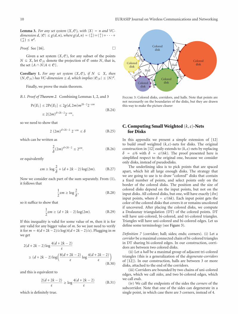
10 EURASIP Journal on Wireless Communications and Networking
Lemma 3. For any set system (X , C), with |X| = n and VC-dimension d, |C| ≤ g(d,n), where g(d,n) = ( n0 )+( n1 )+· · ·+( nd
) ≤ nd.
Proof. See [16].
Given a set system (X , C), for any subset of the pointsN ⊆ X , let C|N denote the projection of C onto N , that is,the set {A∩N|A ∈ C}.
Corollary 1. For any set system (X , C), if N ⊆ X , then(N , C|N ) has VC-dimension ≤ d, which implies |C|N | ≤ |N|d.
Finally, we prove the main theorem.
B.1. Proof of Theorem 2. Combining Lemmas 1, 2, and 3
Pr[E1] ≤ 2Pr[E2] ≤ 2g(d, 2m)m2k−22−εm
≤ 2(2m)d+2k−22−εm,(B.24)
so we need to show that
2 (2m)d+2k−2 2−εm ≤ δ (B.25)
which can be written as
2δ
(2m)d+2k−2 ≤ 2εm. (B.26)
or equivalently
εm ≥ log2δ
+ (d + 2k − 2) log(2m). (B.27)
Now we consider each part of the sum separately. From (1),it follows that
12εm ≥ log
2δ
, (B.28)
so it suffice to show that
12εm ≥ (d + 2k − 2) log(2m). (B.29)
If this inequality is valid for some value of m, then it is forany valid for any bigger value of m. So we just need to verifyit for m = 4(d+ 2k− 2)/ε log(4(d+ 2k− 2)/ε). Plugging in mwe get
2(d + 2k − 2) log4(d + 2k − 2)
ε
≥ (d + 2k − 2) log(
8(d + 2k − 2)ε
log4(d + 2k − 2)
ε
)
(B.30)
and this is equivalent to
2(d + 2k − 2)ε
≥ log4(d + 2k − 2)
ε(B.31)
which is definitely true.
Coloreddisk
Corridor
Hall
Coloreddisk
Corridor
Coloreddisk
Corridor
Coloreddisk
Corridor
Coloreddisk
Cor
rido
r
Hall
Figure 3: Colored disks, corridors, and halls. Note that points arenot necessarily on the boundaries of the disks, but they are drawnthis way to make the picture clearer
C. Computing Small Weighted (k, ε)-Netsfor Disks
In this appendix we present a simple extension of [12]to build small weighted (k, ε)-nets for disks. The originalconstruction in [12] easily extends to (k, ε)-nets by replacingδ = ε/6 with δ = ε/(6k). The proof presented here issimplified respect to the original one, because we consideronly disks, instead of pseudodisks.
The underlining idea is to pick points that are spacedapart, which hit all large enough disks. The strategy thatwe are going to use is to draw “colored” disks that containa fixed number of points, and select points only on theborder of the colored disks. The position and the size ofcolored disks depend on the input points, but not on theinput disks. All colored disks, but one, will have exactly �δn�input points, where δ = ε/(6k). Each input point gets thecolor of the colored disks that covers it or remains uncoloredif uncovered. After placing the colored disks, we computea Dealaunay triangulation (DT) of the colored points. DTwill have uni-colored, bi-colored, and tri-colored triangles.Triangles will have uni-colored and bi-colored edges. Let usdefine some terminology (see Figure 3).
Definition 7 (corridor; hall; sides; ends; corners). (i) Let acorridor be a maximal connected chain of bi-colored trianglesin DT sharing bi-colored edges. In our construction, corri-dors are between two colored disks.
(ii) Let a hall be a maximal group of adjacent tri-coloredtriangles (this is a generalization of the degenerate-corridorsof [12]). In our construction, halls are between 3 or moredisks, attached to the end of the corridors.
(iii) Corridors are bounded by two chains of uni-colorededges, which we call sides, and two bi-colored edges, whichwe call ends.
(iv) We call the endpoints of the sides the corners of thesubcorridor. Note that one of the sides can degenerate in asingle point, in which case there are 3 corners, instead of 4.

EURASIP Journal on Wireless Communications and Networking 11
1 Let δ = ε/(6k);2 Let X1, . . . ,Xj be disjoints subsets of X with the following properties:
− conv(X) ⊆ ⋃1≤i≤ j Xi (where conv is the convex hull)− each Xi is representable as X ∩Hi for some halfplaneHi (or equivalently, Xi = X ∩Di for some (large enough) This construction of subsets of X can be done bydisk Di, and to simplify the proof we can think that Di is bigger than any input disk)− |Xi| = �δn� for 1 ≤ i < j, and |Xj| ≤ �δn�
repeatedly “biting off” subsets of X with halfplanes3 Let Xi+1, . . . ,Xr be a maximal collection of disjoint subsets of X \⋃1≤i≤ j Xi satisfying:
− Xi = X ∩Di for some disk Di
− |Xi| = �δn� for j < i ≤ r;4 For each i, 1 ≤ i ≤ r, color the points of Xi with color i, and call Di the disk defining color i, or colored disk i.
Let X be the set of colored points, and call the points in X \ Xcolorless;5 Let DT be the Dealaunay triangulation of the set of colored points X ;6 Break each corridor C into a minim number of subcorridors, i.e. subchains of the chain of triangles
that form C, so that each subcorridor contains at most �δn� colorless points7 Let N be the set of the corners of all subcorridors. Clearly N ⊂ X ;8 Return N has the (k, ε)-net for D ;
Algorithm 2: Small (k, ε)-nets for disks.
We start by describing the algorithm for the unweightedcase, and we will show how to add weights afterwords. Weare given 0 < ε ≤ 1, a family D of disks, and a set X of n > 2points in the plane. For simplicity assume that the points arein general position (i.e., no three points are collinear, andno four points are cocircular). Let define δ = ε/(6k) (thereason for this will be clear soon). Let X1, . . . ,Xj be disjointssubsets of X constructed in the following manner. From theboundary of X , “bite off” subsets of X of size �δn� with thefollowing properties.
(i) The union of all the Xi subsets contains the boundarypoints of X : conv(X) ⊆ ⋃
1≤i≤ j Xi (where conv is theconvex hull).
(ii) Each Xi is representable as X∩Hi for some half-planeHi (or equivalently, Xi = X ∩ Di for some (largeenough) disk Di, and to simplify the proof we canthink that Di is bigger than any input disk).
(iii) |Xi| = �δn� for 1 ≤ i < j, and |Xj| ≤ �δn�.
Now, consider the internal points of X , that are not partof any disk Xi. We are going to draw the largest number ofdisks of size �δn� to cover the internal points. Specifically,let Xi+1, . . . ,Xr be a maximal collection of disjoint subsets ofX \⋃1≤i≤ j Xi satisfying
(i) Xi = X ∩Di for some disk Di,
(ii) |Xi| = �δn� for j < i ≤ r.
At this point, we have a total of r disks Xi. For each i, 1 ≤i ≤ r, color the points of Xi with color i, and call Di the diskdefining color i, or colored disk i. Let X be the set of coloredpoints, and call the points in X \ Xcolorless. Let DT be theDealaunay triangulation of the set of colored points X . Breakeach corridor C into a minim number of subcorridors, that is,subchains of the chain of triangles that form C, so that eachsubcorridor contains at most �δn� colorless points. Let N be
the set of the corners of all subcorridors. Clearly N ⊂ X . Weare going to show that N is a the (k, ε)-net for D that is, anydisk of D that contains εn points of X also contains k pointsof N . This construction is summarized in Algorithm 2.
First of all note that colorless points can only bein corridors and halls (because unicolored triangles arecontained in the corresponding color-defining disks). Also,we can observe that any disk D ∈ D containing no coloredpoints contains less than �δn� points of X . In fact, fromthe maximality of the construction, there cannot be colorlessdisks with �δn� points. Than we claim what follows.
Claim. There are at most 3r − 6 corridors in DT, and r ≤�1/δ� + 1.
Proof. See [12]. Note that, since all Xi are disjoint, and all butmaybe one contain �δn� points, so r ≤ �1/δ� + 1.
We now prove the (k, ε)-net theorem for disks.
Theorem 5 ((k, ε)-net theorem for disks). Algorithm 2 cre-ates a (k, ε)-net of size O(k/ε) for (X , D), where X is a set ofpoints (|X| > 2) in non-D-degenerate position (i.e., no threepoints are collinear, and no four points are cocircular), and D isa family of disks.
Proof. By claim C we have that the size of N is O(k/ε). So weonly need to show that N contains at least k points in eachinput disk of size at least εn.
First of all, the case k = 1 is already proved in [12], so wefocus on the case of k ≥ 2.
For a generic input disk of size at least εn, we are goingto compute the minimum number of corners contributed byeach intersecting region (colored disk, subcorridor, or hall),while assuming that it has the largest possible intersection.Also, we will pay attention not to count the same cornermultiple times. If a colored disk is completely contained

12 EURASIP Journal on Wireless Communications and Networking
in an input disk, it will contribute for the biggest numberof corners. So we should only consider colored disks thatintersect the boundary of the input disk. We claim that theminimum contribution is given when the boundary of aninput disk intersects an alternation of colored disks andcorridors. In this case we should count 1 corner, for eachcolored disk/corridor. The only case in which (a part of) theboundary of the input disk does not intersect any coloreddisk is when it is contained inside a corridor. But this can onlyhappen if there is a colored disk inside the input disk, but wealready argued that this will give a higher contribution. Thefollowing is an upper bound on the number of intersectingpoints. There can be δn points for the colored disk, plusanother δn points for the subcorridor on the side of thecorner that we are counting, plus another δn points for thehall adjacent to them. This means that for 3δn points there isat least 1 corner. We are considering input disks of size at leastεn = 6kδn, and this implies that there are at least k points ineach disk.
Finally, we consider the weighted case. The constructionis similar to the unweighted one, with the only difference thatthe colored disks contain �δw(X)� points, where w(X) is thesum of the weights of all points. It is easy to see that the prooffollows through.
Acknowledgments
This work was supported in part by the NSF awards:0713186, 0721701, 0721665.
References
[1] H. Gupta, Z. Zhou, S. R. Das, and Q. Gu, “Connected sensorcover: self-organization of sensor networks for efficient queryexecution,” IEEE/ACM Transactions on Networking, vol. 14, no.1, pp. 55–67, 2006.
[2] K. Chakrabarty, S. S. Iyengar, H. Qi, and E. Cho, “Gridcoverage for surveillance and target location in distributedsensor networks,” IEEE Transactions on Computers, vol. 51, no.12, pp. 1448–1453, 2002.
[3] S. Slijepcevic and M. Potkonjak, “Power efficient organizationof wireless sensor networks,” in Proceedings of the InternationalConveference of Communication (ICC ’01), vol. 2, pp. 472–476,Helsinki, Finland, June 2001.
[4] S. Meguerdichian, F. Koushanfar, G. Qu, and M. Potkonjak,“Exposure in wireless ad-hoc sensor networks,” in Proceedingsof the 7th Annual International Conference on Mobile Com-puting and Networking (MOBICOM ’01), pp. 139–150, Rome,Italy, July 2001.
[5] T. H. Cormen, C. E. Leiserson, R. L. Rivest, and C. Stein,Introduction to Algorithms, MIT Press, Boston, Mass, USA, 2ndedition, 2001.
[6] H. Bronnimann and M. T. Goodrich, “Almost optimal setcovers in finite VC-dimension,” Discrete and ComputationalGeometry, vol. 14, no. 1, pp. 463–479, 1995.
[7] D. Haussler and E. Welzl, “ε-nets and simplex range queries,”Discrete and Computational Geometry, vol. 2, no. 1, pp. 127–151, 1987.
[8] M. Hefeeda and M. Bagheri, “Randomized k-coverage algo-rithms for dense sensor networks,” in Proceedings of the 26th
IEEE International Conference on Computer Communications(INFOCOM ’07), pp. 2376–2380, May 2007.
[9] F. Ye, G. Zhong, J. Cheng, S. Lu, and L. Zhang, “PEAS: a robustenergy conserving protocol for long-lived sensor networks,”in Proceedings of the 23rd IEEE International Conferenceon Distributed Computing Systems (ICDCS ’03), pp. 28–37,Providence, RI, USA, May 2003.
[10] S. Shakkottai, R. Srikant, and N. Shroff, “Unreliable sensorgrids: coverage, connectivity and diameter,” in Proceedings ofthe 22nd Annual Joint Conference of the IEEE Computer andCommunications Societies (INFOCOM ’03), vol. 2, pp. 1073–1083, San Francisco, Calif, USA, March-April 2003.
[11] Z. Zhou, S. Das, and H. Gupta, “Connected K-coverageproblem in sensor networks,” in Proceedings of the 13thInternational Conference on Computer Communications andNetworks (ICCCN ’04), pp. 373–378, 2004.
[12] J. Matousek, R. Seidel, and E. Welzl, “How to net a lot withlittle: small ε-nets for disks and halfspaces,” in Proceedings ofthe 6th Annual Symposium on Computational Geometry (SCG’90), pp. 16–22, Berkeley, Calif, USA, June 1990.
[13] J. O’Rourke, Art Gallery Theorems and Algorithms, vol. 3of International Series of Monographs on Computer Science,Oxford University Press, New York, NY, USA, 1987.
[14] P. Valtr, “Guarding galleries where no point sees a small area,”Israel Journal of Mathematics, vol. 104, pp. 1–16, 1998.
[15] G. Fusco and H. Gupta, “Selection and orientation ofdirectional sensors for coverage maximization,” in Proceedingsof the 6th Annual IEEE Conference on Sensor, Mesh and Ad HocCommunications and Networks (SECON ’09), Rome, Italy, June2009.
[16] N. Alon and J. H. Spencer, “ε-nets and VC-dimensions ofrange spaces,” in The Probabilistic Method, pp. 220–225, Wiley-Interscience, New York, NY, USA, 2nd edition, 2000.

Hindawi Publishing CorporationEURASIP Journal on Wireless Communications and NetworkingVolume 2010, Article ID 534712, 10 pagesdoi:10.1155/2010/534712
Research Article
SPM: Source Privacy for Mobile Ad Hoc Networks
Jian Ren, Yun Li, and Tongtong Li
Department of Electrical and Computer Engineering, Michigan State University, East Lansing, MI 48864-1226, USA
Correspondence should be addressed to Jian Ren, [email protected]
Received 2 September 2009; Accepted 21 September 2009
Academic Editor: Benyuan Liu
Copyright © 2010 Jian Ren et al. This is an open access article distributed under the Creative Commons Attribution License, whichpermits unrestricted use, distribution, and reproduction in any medium, provided the original work is properly cited.
Source privacy plays a key role in communication infrastructure protection. It is a critical security requirement for many missioncritical communications. This is especially true for mobile ad hoc networks (MANETs) due to node mobility and lack of physicalprotection. Existing cryptosystem-based techniques and broadcasting-based techniques cannot be easily adapted to MANETbecause of their extensive cryptographic computation and/or large communication overhead. In this paper, we first propose anovel unconditionally secure source anonymous message authentication scheme (SAMAS). This scheme enables message senderto transmit messages without relying on any trusted third parties. While providing source privacy, the proposed scheme canalso provide message content authenticity. We then propose a novel communication protocol for MANET that can ensurecommunication privacy for both message sender and message recipient. This protocol can also protect end-to-end routing privacy.Our security analysis demonstrates that the proposed protocol is secure against various attacks. The theoretical analysis andsimulation show that the proposed scheme is efficient and can provide high message delivery ratio. The proposed protocol canbe used for critical infrastructure protection and secure file sharing in mobile ad hoc networks where dynamic groups can beformed.
1. Introduction
The decentralized nature of mobile ad hoc networks(MANETs) makes rapid deployment of independent mobileusers practical. MANETs are suitable for many applications,such as establishing survivable, dynamic communicationfor emergency/rescue operations, disaster relief efforts, andmilitary networks. MANETs consist of autonomous col-lection of mobile users that communicate over bandwidthconstrained wireless links. All these issues make security,jamming protection, and even node capture significantconcerns. Without privacy protection, adversaries can easilylearn the identities of the communication parties and therelevant information that two users are communicating. Forexample, the adversaries can track your on-line orders, theweb sites that you access, the doctors that you visit and manymore. Adversaries can also easily overhear all the messages,passively eavesdrop on communications and perform trafficanalysis, routing monitoring, and denial-of-service (DoS)attacks.
For a tactical military communication networks, com-munication privacy is becoming an essential security require-
ment. As an example, an abrupt change in traffic patternor volume may indicate some forthcoming activities. Theexposure of such information could be extremely dangerousin that adversaries can easily identify critical network nodesand then launch direct DoS attacks on them. Communica-tion privacy is also an indispensable security requirement forapplications such as e-voting, e-cash and so on.
In the past two decades, originated largely from Chaum’smixnet [1] and DC-net [2], a number of privacy-preservingcommunication protocols have been proposed, includingfor example, onion routing [3], K-anonymous messagetransmission [4], Web MIXes [5], Mixminion [6], Mixingemail [7], Mixmaster Protocol [8], Crowds [9], and Busesseat allocation [10], to name a few. The mixnet familyprotocols use a set of “mix” servers that mix the receivedpackets to make the communication parties (including thesender and the recipient) ambiguous. They rely on thestatistical properties of background traffic that is also referredto as cover traffic to achieve the desired source privacy.The DC-net family protocols [2, 4, 11, 12] on the otherhand, utilize secure multiparty computation techniques.They provide provable source privacy without relying on

2 EURASIP Journal on Wireless Communications and Networking
trusted third parties. However, to broadcast a message, eachparty of the group that the message sender hides, called theambiguity set (AS), needs to choose a random position. Evenif all parties are honest, there are no effective noninteractivemeans that can enable players to select distinct messagepositions. This means that multiple parties may transmitmessages in the same slot. This is called the transmissioncollision problem. There is no existing practical solution tosolve this problem [12].
As the computing, communicating, and cryptographictechniques progress rapidly, increasing emphasis has beenplaced on developing new efficient and secure anonymouscommunication schemes and network protocols withoutrelying on trusted third parties and free of collision.
In this paper, we first propose a novel unconditionallysecure source anonymous message authentication scheme(SAMAS). While providing source privacy, the proposedscheme can also provide message content authenticity with-out relying on any trusted third parties. We then propose anovel communication protocol for MANET that can ensurecommunication privacy for both communication parties andtheir end-to-end communications. The proposed networkprotocol can be used for critical information distribution,infrastructure protection, and secure file sharing. Our secu-rity analysis demonstrates that the proposed protocol issecure against various attacks. The theoretical analysis andsimulation results show that the proposed scheme is efficientand can ensure high message delivery ratio.
The rest of this paper is organized as follows. In Section 2,the terminology, assumptions, and previous relatedworks are briefly reviewed. The proposed unconditionallysecure source anonymous message authentication scheme(SAMAS) and security analysis are described in Section 3.In Section 4, we propose an anonymous communicationprotocol in detail along with security analysis and simulationresults in Section 5. Finally, Section 6 concludes thispaper.
2. Terminology and Preliminary
In this section, we will briefly describe the terminology thatwill be used in this paper. Then we will introduce somecryptographic tools that will be used in this paper. Finally,we will present a brief overview of the related works in thisarea.
2.1. Terminology. Privacy is sometimes referred to asanonymity. Communication anonymity in informationmanagement has been discussed in a number of previousworks [1, 2, 9, 13–15]. It generally refers to the state of beingnot identifiable within a set of subjects. This set is called theambiguity set (AS). Three types of anonymity were defined[13]: sender anonymity, recipient anonymity, and relation-ship anonymity. Sender anonymity means that a particularmessage is not linkable to any sender and no message iflinkable to a particular sender. Recipient anonymity similarlymeans that a message cannot be linked to any recipientand that no message is linkable to a recipient. Relationship
Table 1: Notation.
AS or S Ambiguity set
SAMAS source anonymous message authentication code
MACi ith message authentication code
MES modified ElGamal signature
PPT probabilistic polynomial time
p a large prime number
Zp integer field module p
g a primitive element in Zpxi private key of the ith user
yi public key of the ith user for SAMAC generation
ri ith signature component
s ElGamal signature component
m Message
n number of users in the AS
Ai ith member in the AS
h hash function
hi hash value h(m, ri)
pki(m) encrypt m using public key yiski Ai’s secret key for symmetric encryption
ski(m) encrypt m using secret key skiNi ith nonce
mFi ith message flag
rFi ith recipient flag
‖ message concatenation
M(i, j) message to send from node i to node j
S(m) SAMAC of message m
anonymity means that the sender and the recipient areunlinkable. In other words, sender and recipient cannot beidentified as communicating with each other, though it maybe clear they are participating in some communications.Relationship anonymity is a weaker property than thatof sender anonymity and recipient anonymity. The aboveanonymities are also referred to as the full anonymities, sincethey guarantee that an adversary cannot infer anything aboutthe sender, the recipient, or the communication relationshipfrom a transmitted message.
We will start with the definition of unconditionallysecure source anonymous message authentication scheme(SAMAS).
Definition 1 (SAMAS). An SAMAS consists of the followingtwo algorithms:
(i) generate (m, y1, y2, . . . , yn): Given a message m andthe public keys y1, y2, . . . , yn of the ambiguity set(AS) S = {A1,A2, . . . ,An}, the actual message senderAt, 1 ≤ t ≤ n, produces an anonymous message S(m)using her own private key xt;
(ii) verify S(m): Given a message m and an anonymousmessage S(m), which includes the public keys of allmembers in the AS, a verifier can determine whetherS(m) is generated by a member in the AS.

EURASIP Journal on Wireless Communications and Networking 3
The security requirements for SAMAS include
(i) Sender ambiguity: The probability that a verifiersuccessfully determines the real sender of the anony-mous message is exactly 1/n, where n is the totalnumber of AS;
(ii) Unforgeability: An anonymous message scheme isunforgeable if no adversary, given the public keys ofall members of the AS and the anonymous messagesm1,m2, . . . ,ml adaptively chosen by the adversary,can produce in polynomial time a new valid anony-mous message with nonnegligible probability.
In this paper, the user ID and user public key will be usedinterchangeably without making any distinguish.
2.2. Modified ElGamal Signature Scheme (MES).
Definition 2 (MES). The modified ElGamal signaturescheme [16] consists of the following three algorithms:
(i) Key generation algorithm: Let p be a large prime, gbe a generator of Z∗p . Both p and g are made public.For a random private key x ∈ Zp, the public key y iscomputed from y = gx mod p;
(ii) Signature algorithm: The MES can also have manyvariants [17, 18]. For the purpose of efficiency, we willdescribe the variant, called optimal scheme. To sign amessage m, one chooses a random k ∈ Z∗p−1, thencomputes the exponentiation r = gk mod p andsolves s from
s = rxh(m, r) + k mod(p − 1
), (1)
where h is a one-way hash function. The signature of messagem is defined as the pair (r, s);
(iii) Verification algorithm: The verifier checks the signa-ture equation gs = r yrh(m,r) mod p. If the equalityholds true, then the verifier accepts the signature andre jects otherwise.
2.3. Previous Work. The existing anonymous communica-tion protocols are largely stemmed from either mixnet [1]or DC-net [2]. A mixnet provides anonymity via packetreshuffling through (at least one trusted) “mix”. In amixnet, a sender encrypts an outgoing message and theID of the recipient using the public key of the mix. Themix accumulates a batch of encrypted messages, decryptsand reorders these messages, and forwards them to therecipients. An eavesdropper cannot link a decrypted outputmessage with any particular (encrypted) input message. Themixnet thus protects the secrecy of users’ communicationrelationships. Recently, Moler presented a secure public-keyencryption algorithm for mixnet [19]. This algorithm hasbeen adopted by Mixminion [6]. However, since mixnet-like protocols rely on the statistical properties of backgroundtraffic, they cannot provide provable anonymity.
DC-net [2, 15] is an anonymous multiparty computationamongst a set of participants, some pairs of which sharesecret keys. DC-net provides perfect (information theoretic)sender anonymity without requiring trusted servers. In aDC-net, users send encrypted broadcasts to the entire group,thus achieving receiver anonymity. However, all membersof the group are made aware of when a message is sent,so DC-net does not have the same level of sender-receiveranonymity. Also, in DC-net, only one user can send at a time,so it takes additional bandwidth to handle collisions andcontention. Lastly, a DC-net participant fixes its anonymityversus bandwidth trade off when joining the system, andthere are no provisions to rescale that trade off when othersjoin the system.
Crowds [9] extends the idea of anonymizer and isdesigned for anonymous web browsing. However, Crowdsonly provides sender anonymity. It does not hide thereceivers and the packet content from the nodes en route.Hordes [20] builds on the Crowds. It uses multicast servicesand provides only sender anonymity.
Recently, message sender anonymity based on ringsignatures was introduced [21]. This approach can enablemessage sender to generate source anonymous messagesignature with content authenticity assurance, while hidingthe real identity of the message sender. The major idea isthat the message sender (say Alice) randomly selects n ofring members as the AS on her own without awarenessof these members. To generate a ring signature, for eachmember in the ring other than the actual sender (Alice),Alice randomly selects an input and computes the one-wayoutput using message signature forgery. For the trapdoorone-way function corresponding to the actual sender Alice,she needs to solve the “message” that can “glue” the ringtogether, and then signs this “message” using her knowledgeof the trap-door information. The original scheme has verylimited flexibility and the complexity of the scheme is quitehigh. Moreover, the original paper only focuses on thecryptographic algorithm, the relevant network issues weretotally left unaddressed.
In this paper, we first propose an unconditionally secureand efficient source anonymous message authenticationscheme based on the modified ElGamal signature scheme.This is because the original ElGamal signature scheme isexistentially forgeable with a generic message attack [22,23]. While the modified ElGamal signature (MES) schemeis secure against no-message attack and adaptive chosen-message attack in the random oracle model [24].
2.4. Threat Model and Assumptions. We assume the par-ticipating MANET nodes voluntarily cooperate with eachother to provide the service. All nodes are potential messageoriginators of anonymous communications. The adversariescan collaborate to passively monitor and eavesdrop everyMANET traffic. In addition, they may compromise anynode in the target network to become an internal adversary,which could be the internal perpetrators. In this paper,we assume that passive adversaries can only compromise afraction of the nodes. We also assume that the adversaries are
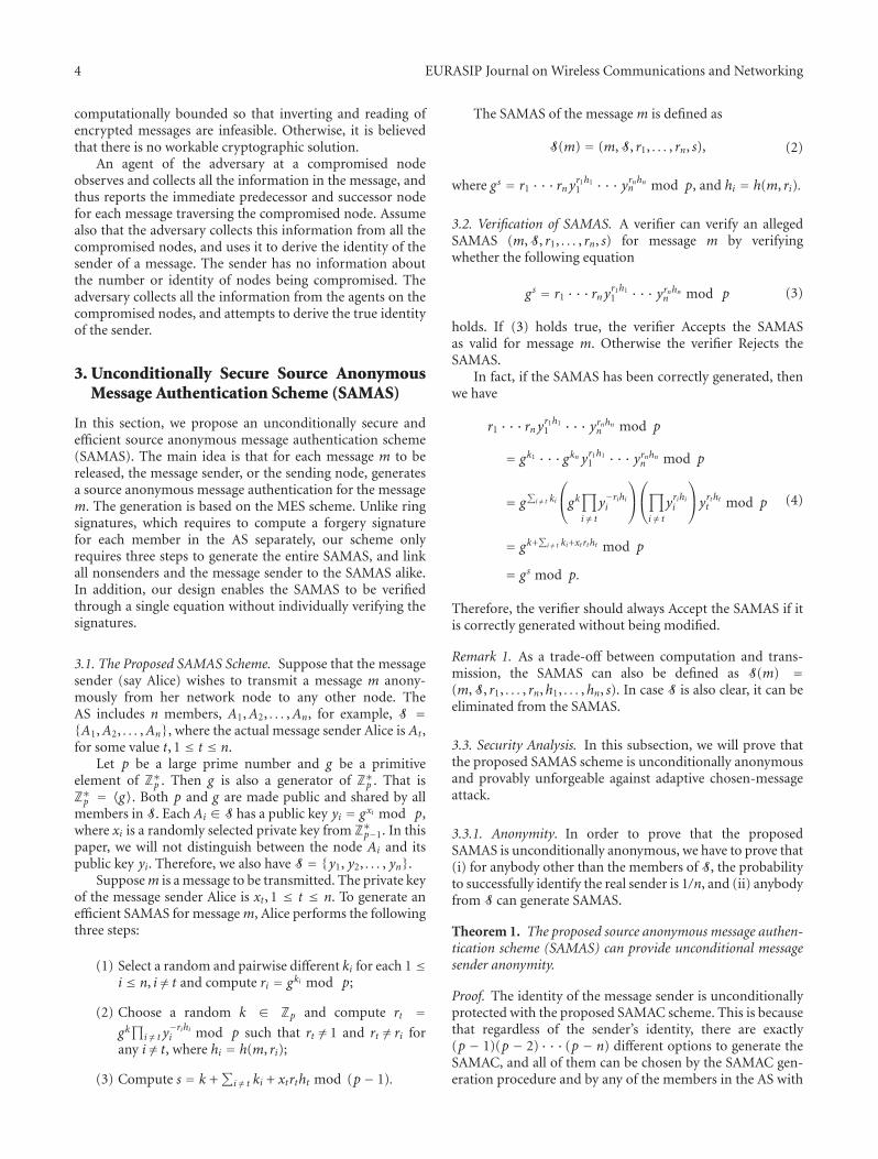
4 EURASIP Journal on Wireless Communications and Networking
computationally bounded so that inverting and reading ofencrypted messages are infeasible. Otherwise, it is believedthat there is no workable cryptographic solution.
An agent of the adversary at a compromised nodeobserves and collects all the information in the message, andthus reports the immediate predecessor and successor nodefor each message traversing the compromised node. Assumealso that the adversary collects this information from all thecompromised nodes, and uses it to derive the identity of thesender of a message. The sender has no information aboutthe number or identity of nodes being compromised. Theadversary collects all the information from the agents on thecompromised nodes, and attempts to derive the true identityof the sender.
3. Unconditionally Secure Source AnonymousMessage Authentication Scheme (SAMAS)
In this section, we propose an unconditionally secure andefficient source anonymous message authentication scheme(SAMAS). The main idea is that for each message m to bereleased, the message sender, or the sending node, generatesa source anonymous message authentication for the messagem. The generation is based on the MES scheme. Unlike ringsignatures, which requires to compute a forgery signaturefor each member in the AS separately, our scheme onlyrequires three steps to generate the entire SAMAS, and linkall nonsenders and the message sender to the SAMAS alike.In addition, our design enables the SAMAS to be verifiedthrough a single equation without individually verifying thesignatures.
3.1. The Proposed SAMAS Scheme. Suppose that the messagesender (say Alice) wishes to transmit a message m anony-mously from her network node to any other node. TheAS includes n members, A1,A2, . . . ,An, for example, S ={A1,A2, . . . ,An}, where the actual message sender Alice is At,for some value t, 1 ≤ t ≤ n.
Let p be a large prime number and g be a primitiveelement of Z∗p . Then g is also a generator of Z∗p . That isZ∗p = 〈g〉. Both p and g are made public and shared by allmembers in S. Each Ai ∈ S has a public key yi = gxi mod p,where xi is a randomly selected private key from Z∗p−1. In thispaper, we will not distinguish between the node Ai and itspublic key yi. Therefore, we also have S = {y1, y2, . . . , yn}.
Supposem is a message to be transmitted. The private keyof the message sender Alice is xt, 1 ≤ t ≤ n. To generate anefficient SAMAS for messagem, Alice performs the followingthree steps:
(1) Select a random and pairwise different ki for each 1 ≤i ≤ n, i /= t and compute ri = gki mod p;
(2) Choose a random k ∈ Zp and compute rt =gk∏
i /= t y−rihii mod p such that rt /= 1 and rt /= ri for
any i /= t, where hi = h(m, ri);
(3) Compute s = k +∑
i /= t ki + xtrtht mod (p − 1).
The SAMAS of the message m is defined as
S(m) = (m, S, r1, . . . , rn, s), (2)
where gs = r1 · · · rnyr1h11 · · · yrnhnn mod p, and hi = h(m, ri).
3.2. Verification of SAMAS. A verifier can verify an allegedSAMAS (m, S, r1, . . . , rn, s) for message m by verifyingwhether the following equation
gs = r1 · · · rn yr1h11 · · · yrnhnn mod p (3)
holds. If (3) holds true, the verifier Accepts the SAMASas valid for message m. Otherwise the verifier Rejects theSAMAS.
In fact, if the SAMAS has been correctly generated, thenwe have
r1 · · · rn yr1h11 · · · yrnhnn mod p
= gk1 · · · gkn yr1h11 · · · yrnhnn mod p
= g∑i /= t ki
⎛
⎝gk∏
i /= ty−rihii
⎞
⎠
⎛
⎝∏
i /= tyrihii
⎞
⎠yrthtt mod p
= gk+∑i /= t ki+xtrtht mod p
= gs mod p.
(4)
Therefore, the verifier should always Accept the SAMAS if itis correctly generated without being modified.
Remark 1. As a trade-off between computation and trans-mission, the SAMAS can also be defined as S(m) =(m, S, r1, . . . , rn,h1, . . . ,hn, s). In case S is also clear, it can beeliminated from the SAMAS.
3.3. Security Analysis. In this subsection, we will prove thatthe proposed SAMAS scheme is unconditionally anonymousand provably unforgeable against adaptive chosen-messageattack.
3.3.1. Anonymity. In order to prove that the proposedSAMAS is unconditionally anonymous, we have to prove that(i) for anybody other than the members of S, the probabilityto successfully identify the real sender is 1/n, and (ii) anybodyfrom S can generate SAMAS.
Theorem 1. The proposed source anonymous message authen-tication scheme (SAMAS) can provide unconditional messagesender anonymity.
Proof. The identity of the message sender is unconditionallyprotected with the proposed SAMAC scheme. This is becausethat regardless of the sender’s identity, there are exactly(p − 1)(p − 2) · · · (p − n) different options to generate theSAMAC, and all of them can be chosen by the SAMAC gen-eration procedure and by any of the members in the AS with

EURASIP Journal on Wireless Communications and Networking 5
equal probability without depending on any complexity-theoretic assumptions. The proof for the second part, thatanybody from S can generate the SAMAC is straightforward.This finishes the proof of this theorem.
3.3.2. Unforgeability. The design of the proposed SAMASrelies on the ElGamal signature scheme. Signature schemescan achieve different levels of security. Security againstexistential forgery under adaptive-chosen message attack isthe maximum level of security.
In this section, we will prove that the proposed SAMASis secure against existential forgery under adaptive-chosenmessage attacks in the random oracle model [25]. Thesecurity of our result is based on the well-known dis-crete logarithms problem (DLP), which assumes that thecomputation of discrete logarithm in Zp for large p iscomputationally infeasible. In other words, no efficientalgorithms are known for non-quantum computers.
We will introduce two lemmas first. Lemma 2, or theSplitting Lemma, is a well-known probabilistic lemma fromreference [24]. The basic idea of the Splitting Lemma is thatwhen a subset Z is “large” in a product space X × Y , it willhave many “large” sections. Lemma 3 is a slight modificationof the Forking Lemma presented in [24]. The proof of thistheorem is mainly probability theory related. We will skip theproof of these two lemmas here.
Lemma 2 (The Splitting Lemma). Let Z ⊂ X × Y such thatPr[(x, y) ∈ Z] ≥ ε. For any α < ε, define W = {(x, y) ∈X ×Y | Pry′∈Y [(x, y′) ∈ Z] ≥ ε−α}, and W = (X ×Y)\W ,then the following statements hold
(1) Pr[W] ≥ α;
(2) ∀(x, y) ∈W , Pry′∈Y [(x, y′) ∈ Z] ≥ ε − α;
(3) Pr[WZ] ≥ α/ε.
Lemma 3 (The Forking Lemma). Let A be a ProbabilisticPolynomial Time (PPT) Turing machine. Given only thepublic data as input, if A can find, with nonnegligible prob-ability, a valid SAMAS (m, S, r1, . . . , rn,h1, . . . ,hn, s) withina bounded polynomial time T , then with nonnegligibleprobability, a replay of this machine which has control overA and a different oracle, outputs another valid SAMAS(m, S, r1, . . . , rn,h′1, . . . ,h′n, s), such that hi = h′i , for all 1 ≤i ≤ n, i /= j for some fixed j.
Theorem 4. The proposed SAMAS is secure against adaptivechosen-message attack in the random oracle model.
Proof. (Sketch) If an adversary can forgery a valid SAMASwith nonnegligible probability, then according to the ForkingLemma, the adversary can get two valid SAMACs
(m, S, r1, . . . , rn,h1, . . . ,hn, s),(m, S, r1, . . . , rn,h′1, . . . ,h′n, s′
),
(5)
such that for 1 ≤ i ≤ n, i /= j,hi = h′i , and hj /=h′j . That is
gs = r1 · · · rn yr1h11 · · · yrnhnn mod p, (6)
gs′ = r1 · · · rn yr1h
′1
1 · · · yrnh′nn mod p. (7)
Divide equations (6) and (7), we obtain
gs−s′ = y
rt(ht−h′t )t mod p. (8)
Equivalently, we have
yt = gs−s′/rt(ht−h′t ) mod p. (9)
Therefore, we can compute the discrete logarithm of ytin base g with nonnegligible probability, which contradictsto the assumption that it is computationally infeasible tocompute the discrete logarithm of yj in base g. Therefore,it is computationally infeasible for any adversary to forge avalid SAMAC.
4. The Proposed Privacy-PreservingCommunication Protocol
4.1. Network Model. Keeping confidential who sends whichmessages, in a world where any physical transmission canbe monitored and traced to its origin, seems impossible.To solve this problem, in this paper, we consider networkswith multiple MANETs. That is, the participating nodes aredivided into a set of small subgroups. We classify the networknodes into two categories, normal nodes and super nodes.A normal node is a network node that may not be ableto communicate direct with the nodes in other MANETs.A super node can be a normal node that can also providemessage forward services to other MANET nodes. It can alsobe a special node dedicated to providing message forwardservices to other MANET nodes. For energy optimization,the normal nodes can take turn to be the super nodes(Figure 1).
Prior to network deployment, there should be an admin-istrator. The administrator is responsible for selection ofsecurity parameters and a group-wise master key sG ∈ Z∗p .The group master key should be well safeguarded fromunauthorized access and never be disclosed to the ordinarygroup members. The administrator then chooses a collision-resistant cryptographic hash function h, mapping arbitraryinputs to fixed-length outputs on Zp, for example, SHA-1[26].
The administrator assigns each super node a sufficientlylarge set of collision-free pseudonyms that can be usedto substitute the real IDs in communications to defendagainst passive attacks. If a super node uses one pseudonymcontinuously for some time, it will not help to defend againstpossible attacks since the pseudonym can be analyzed in thesame way as its real ID. To solve this problem, each nodeshould use dynamic pseudonyms instead. This requires eachsuper node to sign up with the administrator, who will assign

6 EURASIP Journal on Wireless Communications and Networking
Network A
Network B Network C
Super nodeNormal node
Figure 1: An illustration of network topology of the proposedscheme.
each super node a list of random and collision-resistantpseudonyms:
NA ={
idA1 , . . . , idAτ}. (10)
In addition, each super node will also be assigned acorresponding secret set: SA = {gsGh(idA1 ), . . . , gsGh(idAτ )}.
4.2. Anonymous Local MANET Communication. To realizeanonymous network layer communications, obviously thereshould be no explicit information (such as the messagesender and recipient addresses) in the message content.All of the information related to addresses, including thedestination MANET where the recipient resides, should beembedded into the anonymizing message payload.
Prior to network deployment, the administrator needsto select a set of security parameters for the entire system,including a large prime p and a generator g of Z∗p . Thenetwork nodes A1,A2, . . . ,An and the corresponding publickeys y1, y2, . . . , yn of the n participating network nodes,where xi ∈ Zp, is a randomly selected private key of nodeAi, and yi is computed from yi = gxi mod p.
A normal node only communicates to other nodes inthe same MANET. The communication between two normalnodes in different MANETs has to be forwarded through thesupper nodes in the respected local MANETs. Each messagecontains a nonce (N), a message flag (mF), a recipient flag(rF), and a secret key. The nonce is a random number thatis used only once to prevent message replay attack. Therecipient flag enables the recipient to know whether he isthe targeted receiver or a forwarding node. The secret keyis used to encrypt the message payload through symmetricencryption algorithm.
More specifically, for a node Ai to transmit a message manonymously to a node Aj in the same MANET, through the
nodes Ai+1, . . . ,Aj−1, where j > i+1, node Ai generates a newmessage M(i, j) defined in (11),
M(i, j)
= pki+1(Ni+1,mFi+1, rFi+1, ski+1)‖ski+1(M(i + 1, j
))
M(i + 1, j
)
= pki+2(Ni+2,mFi+2, rFi+2, ski+2)‖ski+2(M(i + 2, j
))
...
M(j − 1, j
)
= pkj(Nj ,mFj , rFj , skj
)‖skj(S(m)),
(11)
where for l = i + 1, . . . , j,Nl is a nonce, mFl is a message flag,rFl is a recipient flag, skl is the secret key used for one timemessage encryption, and ‖ stands for message concatenation.
When the node Ai+1 receives the message packet, thenode decrypts the first block of the received message usingits private key corresponding to yi+1. After that, the node willget the recipient flag and message flag with the instructionfor the subsequent actions.
When a message reaches the targeted recipient, to ensuretraffic balance, the node will generate a dummy message toits subsequent nodes. Only the super nodes can terminateor initiate a dummy message. In this way, the amount oftraffic flow that a node creates as the initiator is concealedin the traffic that it forwards since the overall traffic thatit receives is the same as the traffic that it forwards. Inaddition, the message is encrypted with the private key thatonly the recipient can recover. While the intermediate nodescan only view the instruction of the message allowed. Thesender’s message is indistinguishable by other nodes. Thesender and the recipient are thus hidden amongst the othernodes. It is infeasible for the adversary to correlate messagesusing traffic analysis and timing analysis due to messageencryption. Therefore, perfect obscure of its own messagescan be assured. Detailed security analysis will be presentedlater.
Remark 2. When the message is delivered to the recipient’slocal MANET, if the super node is close enough to therecipient node, then the super node can simply broadcastthe message. In this case, the message format in (11) can beadjusted accordingly.
4.3. Dynamic Local MANET Formation. Due to node mobil-ity in the MANET, the local MANET will dynamicallychange over time. This makes reforming of the local MANETan essential part of our proposed scheme. The dynamicupdating of the MANET can be characterized throughmobility of each individual node, that can leave and join alocal MANET.
4.3.1. Process for a Node to Join a Local MANET. When anode, say node Aj , wishes to join a local MANET, it needs

EURASIP Journal on Wireless Communications and Networking 7
to send a request message to the local super node in the formof:
Join Request∥∥∥yj
∥∥∥T, (12)
where yj is the public key of node Aj , and T is a timestamp.After receiving this request message, the super node has todetermine the relative location of this node according tothe direction and strength of the request signal provided bynodes that also received this message. The super node willdetermine where the node should be located in the localMANET logically. Then the super node will broadcast amessage in the following format to inform the local MANETthat node yj will be joining the local MANET in betweennode yi and node yi+1:
Join Confirm∥∥∥yj∥∥∥yi∥∥yi+1
∥∥T , (13)
where T is a timestamp.
4.3.2. Process for a Node to Leave a Local MANET. A nodecan leave a local MANET either positively or passively. Forpositive leaving, the node, say node Aj , is aware that it isleaving the local MANET. It will send a request message tothe local super node in the format of:
Leaving Request∥∥∥yj∥∥∥T , (14)
where yj is the public key of node Aj , and T is a timestamp.For passive leaving, the node will just leave the local MANETwithout informing anyone. The super node will discovera node’s leaving through message transmission failure andHello message detection.
When a super node is aware of a node’s leaving througheither of the two manners, it will inform all of the localMANET members through broadcasting a message:
Leaving Confirm∥∥∥yj∥∥∥T , (15)
which means a node with public key yj has left the localMANET, and it should be removed from the local MANET.
4.4. Anonymous Communications between Two ArbitrarySuper Nodes. In the previous subsections, we present themechanism that allows two arbitrary nodes to communicateanonymously within the same MANET. This includes com-munications between two super nodes in the same MANET.For any two arbitrary super nodes in different MANETsto communicate anonymously, we will first introduce theconcept of anonymous authentication or secret handshakeby Balfanz et al. [27]. Anonymous authentication allows twonodes in the same group to authenticate each other secretly inthe sense that each party reveals its group membership to theother party only if the other party is also a group member.Nonmembers are not able to recognize group members.
The scheme consists of a set of super nodes and anadministrator who creates groups and enrolls super nodesin groups. For this purpose, the administrator will assigneach super node A a set of pseudonyms idA1 , . . . , idAτ , where
τ is a large security parameter. In addition, the administrator
also calculates a corresponding secret set {gsGh(idA1 ) mod
p, . . . , gsGh(idAτ ) mod p} for super node A, where sG is thegroup’s secret and h is a hash function. The pseudonyms willbe dynamically selected and used to substitute the real IDsfor each communication. This means that two super nodes Aand B can know each other’s group membership only if theybelong to the same group.
When the super node A wants to authenticate to thesuper node B, the following secret handshake can beconducted:
(1) A → B: Super node A randomly selects an unusedpseudonym idAi and a random nonce N1, then sendsidAi ,N1 to super node B;
(2) B → A: Super node B randomly selects an unusedpseudonym idBi and a random nonce N2, then sendsidBj ,N2,V0 = h(KBA‖idAi ‖idBj ‖N1‖N2‖0) to super
node A, where KBA = gsGh(idAi )·h(idBj ) mod p;
(3) A → B: Super node A sends V1 =h(KAB‖idAi ‖idBj ‖N1‖N2‖1) to super node B, where
KAB = gsGh(idBj )·h(idAi ) mod p.
Since KBA = KAB, A can verify V0 by checking
whether V0?= h(KAB‖idAi ‖idBj ‖N1‖N2‖0). If the verification
succeeds, then A knows that B is an authentic group
peer. Similarly, B can verify A by checking whether V1?=
h(KBA‖idAi ‖idBj ‖N1‖N2‖1). If the verification succeeds, thenB knows that A is also an authentic group peer. However, inthis authentication process, neither super node A, nor supernode B can get the real identity of the other node. In otherwords, the real identities of super node A and super node Bremain anonymous after the authentication process.
4.5. Anonymous Communication between Two Arbitrary Nor-mal Nodes. As mentioned before, there should be no explicitexposure about the addresses of the message sender andrecipient. To transmit a message, the sender first randomlyselects a local super node and transmits the message tothe super node according to the mechanism describedbefore. On receiving the message, the local super node firstdetermines the destination MANET ID by checking themessage recipient flag rF, either 0 or 1. If it is 0, thenthe recipient and the super node are in the same MANET.The message can be forwarded in the recipient node usingthe previously described mechanism. If rF is 1, then therecipient is in a different MANET, The super node forwardsthe message to a super node in the destination MANETas described in the previous subsection. Finally, when thesuper node in the recipient’s local MANET receives themessage, the communication again becomes local MANETcommunications. The message can now be transmitted in thesame way that the sender and the recipient are in the sameMANET.
While providing message recipient anonymity, the mes-sage can also be encrypted so that only the messagerecipient can decrypt the message. The proposed anonymous

8 EURASIP Journal on Wireless Communications and Networking
communication is quite general and can be used in a varietyof situations for communication anonymity in MANET,including anonymous file sharing.
4.6. Security Analysis. In this subsection, we will analyzeanonymity, impersonation attack, and replay attack of theproposed anonymous communication protocol.
4.6.1. Anonymity. We will first prove that the proposed com-munication protocol can provide both message sender andrecipient anonymity in the local MANET communications.
Theorem 5. It is computationally infeasible for an adversary toidentify the message sender and recipient in the local MANET.Therefore, the proposed anonymous communication protocolprovides both sender and recipient anonymity in the localMANET.
Proof. (Sketch) First, since the number of message packagesthat each node receives from its immediate predecessor isthe same as the number of packets that it forwards to itsimmediate successor, so the adversaries cannot determine themessage source based on the traffic volume or the numberof message packets. Second, since the message packages areencrypted using either the public keys or the shared secretkeys of the intermediate nodes. No adversary is able todistinguish the real meaningful message from the dummymessage in the transmission in any of the network nodesdue to the traffic balance property and message contentencryption. Therefore, the adversary cannot distinguish theinitiator traffic from the indirection traffic and learn whetherthe node is a recipient, a receiver, or simply a node thatprovides message forward service. Consequently, both themessage sender and recipient information is anonymous forthe adversary attack.
For any two normal nodes in different MANETs tocommunicate anonymously, the communication can bebroken into three segments: the communication between thesender and a local super node in the message sender’s localMANET, the communication between two super nodes in thecorresponding MANETs, and the communication betweenthe recipient super node and the recipient. Theorem 5 hasassured the communication anonymity between a supernode and a normal node in the local MANETs. Therefore,we only need to ensure anonymity between two super nodesin different MANETs in order to achieve full anonymitybetween the sender and recipient.
We already described before that each super node is beingassigned a large set of pseudonyms. A dynamically selectedpseudonym will be used for each communication. Thepseudonyms do not carry the user information implicitly.Therefore, the adversary cannot get any information ofthe super nodes from the network. This result can besummarized into the following theorem.
Theorem 6. The proposed communication protocol can pro-vide both message sender and recipient anonymity between anytwo super nodes.
Corollary 7. The proposed anonymous communication proto-col can provide full anonymity for any sender and recipient inthe MANETs.
4.6.2. Impersonation Attacks. For an adversary elected toperform impersonation attack to a normal node, he needsto be able to conduct forgery attack. We already proved inTheorem 4 that this is infeasible. Therefore, we only needto consider whether it is feasible for an adversary to forge asuper node.
For an adversary to impersonate as a super node, heneeds to be able to authenticate himself with a super node A.This requires the adversary A to compute gsGidA·idAi mod p,where idA is the identity of the adversary and idAi is theith pseudonym of the super node A. However, since theadversary does not know the master secret sG, he is unableto compute gsGh(idA)·h(idAi ) mod p and impersonate as a supernode. Therefore, we have the following theorem.
Theorem 8. It is computationally infeasible for a PPT adver-sary A to impersonate as a super node.
Like all other network communication protocols, in ourproposed protocol, an adversary may choose to drop someof the messages. However, if the immediate predecessor andthe successor nodes are honest and willing to cooperate, thenthe messages being dropped, and the substitution of the validmessages with the dummy messages can be effectively trackedusing the provided message flags.
An adversary that is elected as a super node may refuseto forward messages across the MANETs and thus blockthe anonymous communications between the sender andthe receiver. This attack can be hard to detect if the senderdoes not have the capability to monitor all network traffic.However, the sender can randomly select the super nodes foreach data transmission. If the nonce is properly generated,when a packet is lost, the recipient should be able to know.
4.6.3. Message Replay Attacks. The message replay attackoccurs when an adversary can intercept the communicationpacket, correlate the message to the corresponding senderand recipient, and retransmit it. We have the followingtheorem.
Theorem 9. It is computationally infeasible for an adversaryto successfully modify/reply an (honest) node’s message.
Proof (Sketch). According to (11), each message package incommunication has a unique one-time session ID (nonce)to protect the message package from being modified orreplayed. In addition, these fields are encrypted using theintermediate receiver nodes’ public key so that only thedesignated receiver nodes can decrypt the message. Inthis way, each packet transmitted across different MANETsbears different and uncorrelated IDs and content for PPTadversaries. Therefore, it is computationally infeasible for theadversary to modify or replay any messages in the MANET.This includes the case that even if the same message is being

EURASIP Journal on Wireless Communications and Networking 9
0.1
0.2
0.3
0.4
0.5
0.6
0.7
0.8E
ner
gy(j
oule
)
8 10 12 14 16
Interval = 60 sInterval = 90 s
Interval = 120 sInterval = 150 s
Number of nodes in each MANET
(a) Energy consumption of normal nodes
2
4
6
8
10
12
14
16
En
ergy
(jou
le)
8 10 12 14 16
Interval = 60 sInterval = 90 s
Interval = 120 sInterval = 150 s
Number of nodes in each MANET
(b) Energy consumption of super nodes
0.1
0.12
0.14
0.16
0.18
0.2
0.22
0.24
Del
ay(s
econ
ds)
8 10 12 14 16
Interval = 60 sInterval = 90 s
Interval = 120 sInterval = 150 s
Number of nodes in each MANET
(c) Communication delay
0.98
0.985
0.99
0.995
1
Del
iver
yra
tio
8 10 12 14 16
Interval = 60 sInterval = 90 s
Interval = 120 sInterval = 150 s
Number of nodes in each MANET
(d) Message delivery ratio
Figure 2: Simulation results of the proposed secure routing scheme.
transmitted multiple times, the adversary still cannot linkthem together without knowing all the private keys of theintermediate nodes.
5. Performance Analysis and Simulation Results
In this section, we will provide simulation results of ourproposed protocol on energy consumption, communicationdelay, and message delivery ratio. For energy consumption,we provide simulations for both the normal nodes and thesuper nodes. For wireless communications, due to collisionand packet drop, it is very challenging to assure highmessages delivered ratio. However, our simulation resultsdemonstrate that the proposed protocol can achieve highmessage delivery ratio (Figure 2).
Our simulation was performed using ns-2 on Linuxsystem. In the simulation, the target area is a square fieldof size 2000 × 2000 meters. There are 64 rings located inthis area. The number of the nodes on each ring, that is, thering length, is set to be from 7 to 16 in our simulation. Themessage generation interval is set to be four different values:60 seconds, 90 seconds, 120 seconds, and 150 seconds in oursimulation for comparison. The messages transmitted in thenetwork are 512 bytes long.
6. Conclusion
In this paper, we first propose a novel and efficient sourceanonymous message authentication scheme (SAMAS) thatcan be applied to any messages. While ensuring message

10 EURASIP Journal on Wireless Communications and Networking
sender privacy, SAMAS can also provide message contentauthenticity. To provide provable communication privacywithout suffering from transmission collusion problem, wethen propose a novel privacy-preserving communicationprotocol for MANETs that can provide both message senderand recipient privacy protection. Security analysis shows thatthe proposed protocol is secure against various attacks. Ourperformance analysis and simulation results both demon-strate that the proposed protocol is efficient and practical. Itcan be applied for secure routing protection and file sharing.
Acknowledgments
This research is supported in part by NSF grants CNS0845812, CNS 0848569, CNS 0716039 and CNS 0746811.
References
[1] D. Chaum, “Untraceable electronic mail, return addresses, anddigital pseudonyms,” Communications of the ACM, vol. 24, pp.84–88, 1981.
[2] D. Chaum, “The dining cryptographers problemml: uncondi-tional sender and recipient untraceability,” Journal of Cryptol-ogy, vol. 1, no. 1, pp. 65–75, 1988.
[3] M. Reed, P. Syverson, and D. Goldschlag, “Anonymousconnections and onion routing,” IEEE Journal on SelectedAreas in Communications, vol. 16, no. 4, pp. 482–494, 1998.
[4] L. von Ahn, A. Bortz, and N. Hopper, “k-anonymous messagetransmission,” in Proceedings of the 10th ACM Conference onComputer and Communications Security (CCS ’03), pp. 122–130, Washingtion, DC, USA, October 2003.
[5] O. Berthold, H. Federrath, and S. Kopsell, “Web MIXes: asystem for anonymous and unobservable internet access,” inProceedings of the Workshop on Design Issues in Anonymity andUnobservability, vol. 2248 of Lecture Notes in Computer Science,pp. 115–129, 2001.
[6] G. Danezis, R. Dingledine, and N. Mathewson, “Mixminion:design of a type III anonymous remailer protocol,” in Proceed-ings of the IEEE Computer Society Symposium on Research inSecurity and Privacy, pp. 2–15, Oakland, Calif, USA, May 2003.
[7] C. Gulcu and G. Tsudik, “Mixing email with babel,” inProceedings of the Symposium on Network and DistributedSystem Security, San Diego, Calif, USA, February 1996.
[8] U. Moller, L. Cottrell, P. Palfrader, and L. Sassaman, “Mixmas-ter protocol,” Version 2, July 2003.
[9] M. Reiter and A. Rubin, “Crowds: anonymity for webtransaction,” ACM Transactions on Information and SystemSecurity, vol. 1, no. 1, pp. 66–92, 1998.
[10] A. Beimel and S. Dolev, “Buses for anonymous messagedelivery,” Journal of Cryptology, vol. 16, no. 1, pp. 25–39, 2003.
[11] S. Goel, M. Robson, M. Polte, and E. Sirer, “Herbivore: a scal-able and efficient protocol for anonymous communication,”Tech. Rep. 2003-1890, Cornell University, Ithaca, NY, USA,2003.
[12] P. Golle and A. Juels, “Dining cryptographers revisited,” inProceedings of the International Conference on the Theoryand Applications of Cryptographic Techniques (Eurocrypt ’04),Lecture Notes in Computer Science, pp. 456–473, Interlaken,Switzerland, May 2004.
[13] A. Pfitzmann and M. Hansen, “Anonymity, unlinkability,unobservability, pseudonymity, and identity management
a proposal for terminology,” February 2008, http://dud.inf.tu-dresden.de/literatur/Anon Terminology v0.31.pdf.
[14] A. Pfitzmann and M. Waidner, “Networks without userobservability-design options,” in Proceedings of the Workshopon the Theory and Application of Cryptographic Techniques(Eurocrypt ’85), vol. 219 of Lecture Notes in Computer Science,pp. 245–253, Linz, Austria, April 1985.
[15] M. Waidner, “Unconditional sender and recipient untraceabil-ity in spite of active attacks,” in Proceedings of the Workshopon the Theory and Application of Cryptographic Techniques(Eurocrypt ’89), vol. 434 of Lecture Notes in Computer Science,pp. 302–319, Houthalen, Belgium, April 1989.
[16] D. Pointcheval and J. Stern, “Security arguments for digitalsignatures and blind signatures,” Journal of Cryptology, vol. 13,no. 3, pp. 361–396, 2000.
[17] L. Harn and Y. Xu, “Design of generalised ElGamal type digitalsignature schemes based on discrete logarithm,” ElectronicsLetters, vol. 30, no. 24, pp. 2025–2026, 1994.
[18] K. Nyberg and R. A. Rueppel, “Message recovery for signa-ture schemes based on the discrete logarithm problem,” inProceedings of the International Conference on the Theory andApplication of Cryptographic Techniques (Eurocrypt ’95), vol.950 of Lecture Notes in Computer Science, pp. 182–193, Saint-Malo, France, May 1995.
[19] B. Moller, “Provably secure public-key encryption for length-preserving chaumian mixes,” in Proceedings of the Cryptogra-pher’s Track at the RSA Conference (CT-RSA ’03), vol. 2612 ofLecture Notes in Computer Science, pp. 244–262, San Francisco,Calif, USA, April 2003.
[20] C. Shields and B. N. Levine, “A protocol for anonymouscommunication over the Internet,” in Proceedings of the 7thACM Conference on Computer and Communication Security,D. Gritzalis, Ed., ACM Press, Athens, Greece, November 2000.
[21] R. Rivest, A. Shamir, and Y. Tauman, “How to leak a secret,”in Proceedings of the 7th International Conference on theTheory and Application of Cryptology and Information Security(ASIACRYPT ’01), vol. 2248 of Lecture Notes in ComputerScience, Springer, Gold Coast, Australia, December 2001.
[22] T. A. ElGamal, “A public-key cryptosystem and a signaturescheme based on discrete logarithms,” IEEE Transactions onInformation Theory, vol. 31, no. 4, pp. 469–472, 1985.
[23] S. Goldwasser, S. Micali, and R. Rivest, “A digital signaturescheme secure against adaptive chosen-message attacks,”SIAM Journal on Computing, vol. 17, pp. 281–308, 1988.
[24] D. Pointcheval and J. Stern, “Security proofs for signatureschemes,” in Proceedings of the International Conference on theTheory and Application of Cryptographic Techniques (EURO-CRYPT ’96), vol. 1070 of Lecture Notes in Computer Science,pp. 387–398, Saragossa, Spain, May 1996.
[25] M. Bellare and P. Rogaway, “Random oracles are practical: aparadigm for designing efficient protocols,” in Proceedings ofthe 1st ACM Conference on Computer and CommunicationsSecurity (CCS ’93), pp. 62–73, Fairfax, Va, USA, November1993.
[26] F. P. 180-1, “Secure hash standard,” April 1995, http://www.itl.nist.gov/fipspubs/fips180-1.htm.
[27] D. Balfanz, G. Durfee, N. Shankar, D. Smetters, J. Staddon,and H. C. Wong, “Secure handshakes from pairing-based keyagreements,” in Proceedings of the IEEE Symposium on Security& Privacy, Oakland, Calif, USA, May 2003.