winwcp user guide v3.9 - university of...
TRANSCRIPT

Strathclyde Electrophysiology Software Whole Cell Program WCP for Windows V3.9 User Guide (c) John Dempster, 1997-2004 12/2/2004

WinWCP V3.9 User Guide 2
Contents
1. CONDITIONS OF USE..............................................................................................................................5
2. INTRODUCTION & SOFTWARE INSTALLATION ......................................................................6 2.1. INSTALLATION PROCEDURE..................................................................................................................7 2.2. INSTALLING THE WINWCP SOFTWARE ..............................................................................................7 2.3. HARDWARE REQUIREMENTS................................................................................................................7 2.4. CAMBRIDGE ELECTRONIC DESIGN INTERFACES...............................................................................8
2.4.1. Software installation...................................................................................................................8 2.4.2. Signal input / output connections..............................................................................................9 2.4.3. Troubleshooting tips................................................................................................................ 10
2.5. NATIONAL INSTRUMENTS INTERFACE CARDS..................................................................................11 2.5.1. Software installation................................................................................................................ 11 2.5.2. Signal input / output connections........................................................................................... 12 2.5.3. Troubleshooting........................................................................................................................ 13
2.6. AXON INSTRUMENTS DIGIDATA 1200 ..............................................................................................14 2.6.1. Software Installation............................................................................................................ 14 2.6.2. Signal input / output connections........................................................................................... 15 2.6.3. Troubleshooting..................................................................................................................... 15
2.7. AXON INSTRUMENTS DIGIDATA 1320 SERIES.................................................................................16 2.7.1. Software Installation................................................................................................................ 16 2.7.2. Signal input / output connections........................................................................................... 17 2.7.3. Troubleshooting..................................................................................................................... 17
2.8. INSTRUTECH ITC-16/18 ......................................................................................................................18 2.8.1. Instrutech ITC-16/18 – I/O Panel Connections.................................................................. 18 2.8.2. Installing software support for the Instrutech ITC-16/18.................................................. 19 2.8.3. Instrutech ITC-16/18 : Troubleshooting............................................................................... 19
3. USING WCP - AN OVERVIEW ........................................................................................................... 20
4. CONNECTING WINWCP TO YOUR EXPERIMENT ................................................................ 21 4.1. EXAMPLE 1 - CONNECTING WINWCP TO A PATCH CLAMP ...........................................................21 4.2. EXAMPLE 2 – RECORDING ENDPLATE POTENTIALS WITH WINWCP ...........................................22
5. CONFIGURING WINWCP FOR A RECORDING SESSION .................................................... 24 5.1. CREATING A DATA FILE.......................................................................................................................24 5.2. SETTING RECORDING PARAMETERS...................................................................................................24
5.2.1. No. Channels............................................................................................................................. 24 5.2.2. Record Duration....................................................................................................................... 25 5.2.3. No. Samples/Channel............................................................................................................... 25 5.2.4. Sampling Interval ..................................................................................................................... 25 5.2.5. A/D Converter Voltage Range................................................................................................ 25 5.2.6. Time Units.................................................................................................................................. 25 5.2.7. Channel Calibration Table..................................................................................................... 26 5.2.8. Amplifiers................................................................................................................................... 26
6. MONITORING INPUT SIGNALS & PATCH PIPETTE SEAL TEST.................................... 27 6.1. SELECT CURRENT AND VOLTAGE CHANNELS...................................................................................27 6.2. COMMAND VOLTAGE DIVIDE FACTOR...............................................................................................27 6.3. CELL HOLDING VOLTAGE AND TEST PULSES....................................................................................27 6.4. CURRENT AND VOLTAGE READOUTS.................................................................................................28 6.5. DISPLAY SCALING AND SWEEP TRIGGERING....................................................................................28
7. MAKING A RECORDING..................................................................................................................... 29 7.1. TRIGGER MODES...................................................................................................................................30
7.1.1. Free Run..................................................................................................................................... 30 7.1.2. External Trigger....................................................................................................................... 30

WinWCP V3.9 User Guide 3
7.1.3. Event Detector........................................................................................................................... 30 7.1.4. Stimulus Program..................................................................................................................... 31
8. CREATING STIMULUS PROTOCOLS............................................................................................ 32 8.1. BUILDING A STIMULUS P ROTOCOL....................................................................................................32 8.2. CREATING A VOLTAGE ST IMULUS WAVEFORM ................................................................................33
8.2.1. Rectangular voltage pulse of fixed size................................................................................. 33 8.2.2. Family of rectangular pulses varying in amplitude............................................................ 33 8.2.3. Family of rectangular voltage pulses varying in duration................................................ 34 8.2.4. Series of rectangular voltage pulses..................................................................................... 34 8.2.5. Voltage ramp ............................................................................................................................. 34 8.2.6. Digitised analogue waveform................................................................................................. 35
8.3. CREATING A DIGITAL ST IMULUS PATTERN.......................................................................................35 8.3.1. Digital pulse (fixed duration)................................................................................................. 36 8.3.2. Family of digital pulse (varying in duration) ...................................................................... 36 8.3.3. Train of digital pulses.............................................................................................................. 37
8.4. COMMAND VOLTAGE DIVIDE FACTOR...............................................................................................37 8.5. RECORDING SWEEP TRIGGER PULSE.................................................................................................37 8.6. LEAK SUBTRACTION ............................................................................................................................37 8.7. PROTOCOL LINKING.............................................................................................................................38 8.8. SAVING AND LOADING ST IMULUS PROTOCOLS................................................................................38 8.9. STIMULUS PROTOCOL EXAMPLES......................................................................................................38
9. VIEWING DIGITISED RECORDS STORED ON FILE. ............................................................. 39 9.1. SELECTING AND DISPLAYING RECORDS............................................................................................39 9.2. MAGNIFYING THE DISPLAY.................................................................................................................39 9.3. PRINTING RECORDS..............................................................................................................................40 9.4. CHOOSING A PRINTER AND OUTPUT FORMAT...................................................................................40 9.5. REJECTING FLAWED RECORDS...........................................................................................................41 9.6. CLASSIFYING RECORDS.......................................................................................................................41 9.7. CURSOR MEASUREMENT OF SIGNAL LEVELS....................................................................................41 9.8. ZERO LEVELS........................................................................................................................................42
9.8.1. From record mode.................................................................................................................... 42 9.8.2. Fixed mode ................................................................................................................................ 42
9.9. COPYING RECORDS TO THE WINDOWS CLIPBOARD........................................................................43 9.9.1. Copying data values................................................................................................................. 43 9.9.2. Copying the displayed image. ................................................................................................ 43
9.10. SMOOTHING THE DISPLAYED RECORDS............................................................................................43 10. AUTOMATIC MEASUREMENT OF SIGNAL WAVEFORMS ........................................... 44
10.1. PREPARATION FOR WAVEFORM ANALYSIS.......................................................................................44 10.2. MAKING WAVEFORM MEASUREMENT S.............................................................................................44 10.3. RUNNING A WAVEFORM ANALYSIS SEQUENCE................................................................................44 10.4. MEASUREMENT VARIABLES...............................................................................................................45 10.5. PLOTTING X/Y GRAPHS OF MEASUREMENT VARIABLES................................................................46
10.5.1. Customising the graph............................................................................................................. 46 10.6. CLASSIFYING RECORDS BY WAVEFORM MEASUREMENT CRITERIA ..............................................46
10.6.1. Printing the graph .................................................................................................................... 47 10.6.2. Copying the graph data points to the Windows clipboard................................................ 47 10.6.3. Copying an image of the graph to the Windows clipboard............................................... 47 10.6.4. Fitting a curve to the graph.................................................................................................... 48
10.7. PLOTTING HISTOGRAMS OF MEASUREMENT VARIABLES................................................................49 10.7.1. Customising histograms.......................................................................................................... 49 10.7.2. Printing the histogram............................................................................................................. 50 10.7.3. Copying the histogram data points to the Windows clipboard......................................... 50 10.7.4. Copying an image of the histogram to the Windows clipboard........................................ 50 10.7.5. Fitting gaussian curves to the histogram............................................................................. 51
10.8. SUMMARIES OF RESULTS. ...................................................................................................................52 10.9. TABULATING LISTS OF RESULTS........................................................................................................52
11. CURVE FITTING................................................................................................................................ 53

WinWCP V3.9 User Guide 4
11.1. INTRODUCTION.....................................................................................................................................53 11.2. FITTING CURVES TO DIGITISED SIGNALS...........................................................................................53 11.3. RUNNING A CURVE FITTING SEQUENCE ............................................................................................54 11.4. CURVE FIT RESULTS.............................................................................................................................55 11.5. PLOTTING AND TABULATING RESULTS.............................................................................................55 11.6. EQUATIONS...........................................................................................................................................56
11.6.1. Assessing the quality of a curve fit ........................................................................................ 57 11.6.2. Does the chosen function provide a good fit to the data?................................................. 57 11.6.3. Are the parameters well-defined?.......................................................................................... 57 11.6.4. Are all the parameters meaningful?...................................................................................... 57
12. SIGNAL AVERAGING...................................................................................................................... 58 12.1. PRINCIPLES OF SIGNAL AVERAGING..................................................................................................58 12.2. CREATING SIGNAL AVERAGES............................................................................................................58 12.3. VIEWING AVERAGED DATA RECORDS...............................................................................................59
13. DIGITAL SUBTRACTION OF LEAK CURRENTS ................................................................ 60 13.1. RECORDING PROTOCOLS FOR LEAK SUBTRACTION.........................................................................60 13.2. SUBTRACTING LEAK CURRENTS.........................................................................................................61
14. NON-STATIONARY NOISE ANALYSIS .................................................................................... 62
15. QUANTAL ANALYSIS OF TRANSMITTER RELEASE....................................................... 64 15.1. QUANTAL CONTENT (DIRECT METHOD)............................................................................................64 15.2. QUANTAL CONTENT (VARIANCE METHOD)......................................................................................64 15.3. QUANTAL CONTENT (FAILURES METHOD).......................................................................................64 15.4. BINOMIAL ANALYSIS...........................................................................................................................64 15.5. CORRECTION FOR NON-LINEAR SUMMATION OF POTENTIALS.......................................................65 15.6. QUANTAL CONTENT CALCULATION PROCEDURE ............................................................................65
16. SYNAPTIC CURRENT DRIVING FUNCTION ANALYSIS ................................................. 67
17. EDITING DIGITISED SIGNAL RECORDS ............................................................................... 69 17.1. SHIFTING THE SIGNAL HORIZONTALLY.............................................................................................69 17.2. SHIFTING THE SIGNAL VERTICALLY..................................................................................................69 17.3. SCALING THE SIGNAL..........................................................................................................................69 17.4. STIMULUS ARTEFACT REMOVAL........................................................................................................69 17.5. UNDOING OR ACCEPTING CHANGES..................................................................................................69
18. DATA FILES ......................................................................................................................................... 70 18.1. OPENING A EXISTING WCP DATA FILE.............................................................................................70 18.2. APPENDING A WCP DATA FILE..........................................................................................................70 18.3. IMPORTING FROM FOREIGN DATA FILE FORMATS............................................................................70
18.3.1. Axon Instruments. ..................................................................................................................... 71 18.3.2. Cambridge Electronic Design................................................................................................ 71 18.3.3. ASCII text files. ......................................................................................................................... 71 18.3.4. Binary data files........................................................................................................................ 72
18.4. EXPORTING TO FOREIGN DATA FILES................................................................................................73 18.5. EXPERIMENT LOG FILE........................................................................................................................73
19. SIMULATIONS .................................................................................................................................... 74 19.1. NERVE-EVOKED EPSCS......................................................................................................................74 19.2. VOLTAGE-ACTIVATED CURRENTS SIMULATION ..............................................................................75 19.3. MINIATURE EPSC SIMULATION........................................................................................................77
20. REFERENCES ...................................................................................................................................... 78
21. APPENDIX: WCP DATA FILE STRUCTURE. ......................................................................... 79

WinWCP V3.9 User Guide 5
1. Conditions of Use
The Strathclyde Electrophysiology Software package is a suite of programs for the acquisition and analysis of electrophysiological signals, developed by the author at the department of Physiology & Pharmacology, University of Strathclyde.
At the discretion of the author, the software is supplied free of charge to academic users and others working for non-commercial, non-profit making, organisations. Commercial organisations may purchase a license to use the software from the University of Strathclyde (contact the author for details).
The author retains copyright and all rights are reserved. The user may use the software freely for their own research, but should not sell or pass the software on to others without the permission of the author.
Except where otherwise specified, no warranty is implied, by either the author or the University of Strathclyde, concerning the fitness of the software for any purpose. The software is supplied "as found" and the user is advised to verify that the software functions appropriately for the purposes that they choose to use it.
An acknowledgement of the use of the software, in publications to which it has contributed, would be gratefully appreciated by the author.
John Dempster Department of Physiology & Pharmacology Strathclyde Institute for Biomedical Sciences University of Strathclyde 27 Taylor St. GLASGOW G4 0NR Scotland Tel (0)141 548 2320 Fax. (0)141 552 2562 E-mail [email protected]

WinWCP V3.9 User Guide 6
2. Introduction & Software Installation
WinWCP is a data acquisition and analysis program for handling signals from whole-cell electrophysiological experiments. These may include whole-cell patch clamp experiments, single- and two-microelectrode voltage-clamp studies, or simple membrane potential recordings. Whole-cell signals are produced by the summation of currents through the (usually) large population of ion channels in the cell membrane, and thus consist of relatively smooth current or potential waveforms. The amplitude and time course of such signals contain information concerning the kinetic behaviour of the underlying ion channels, and other cellular processes, which can be extracted by the application of a variety of waveform analysis techniques.
WinWCP provides, in a single program, the data acquisition and experimental stimulus generation features necessary to make a digital recording of the electrophysiological signals, and a range of waveform analysis procedures commonly applied to such signals. WinWCP acts like a multi-channel digital oscilloscope, collecting series of signal and storing them in a data file on magnetic disk. Its major features are
Recording
• 8 analogue input channels. • 29952 samples per recording sweep. • 2 billion records per data file. • Stimulus voltage waveform generator. • 8 TTL digital output lines, for operating solenoid controlled valves or other experimental
devices. • TTL External trigger input, to synchronise recording sweeps with external events. • Digital valve control pattern generator. • Spontaneous event detector. Analysis • Signal averaging. • Leak current subtraction. • Automatic waveform amplitude/time course measurement. • Mathematical curve fitting to waveforms. • Non-stationary noise analysis. • Quantal analysis of synaptic currents. • Synaptic driving function analysis. • Synaptic current and Hodgkin-Huxley current simulations.

WinWCP V3.9 User Guide 7
2.1. Installation procedure
If you wish to use WinWCP to digitise analogue signals (rather than just analyse existing or simulated data files) you must have one of the laboratory interface cards supported by WinWCP installed in your computer. You must also ensure that the interface card is appropriately configured to work with WinWCP. This may involve setting switches or jumpers on the card itself. With some interfaces the manufacturer’s software support libraries must also be installed and configured before it can be used. The full installation procedure consists of the following steps:
1) Install the WinWCP software (see section 2.2).
2) Install the laboratory interface unit and software (see section 2.4, 2.5, or 2.6).
3) Configure WinWCP to work with laboratory interface
4) Attach analogue input/output signal cables (see section 4).
2.2. Installing the WinWCP software
To install WinWCP:
1) Go to the web page www.strath.ac.uk/Departments/PhysPharm/ses.htm and click the WinWCP V3.x.x Installation Disk option to download a self-extracting archive (WinWCP_Vxxx.exe) containing the WinWCP installation files. Store this file in a temporary folder (e.g. c:\temp) on your computer.
2) Open the temporary folder and double -click the archive to unpack the WinWCP setup program.
3) Start the installation program by double-clicking the program Setup.
The setup program creates the directory c:\Program Files\Strathclyde University\WinWCP and installs the WinWCP programs files within it. (You can change the disk drive and directory if you wish). 4) To start WinWCP, click the Microsoft Windows Start button and select WinWCP
V3.1.x from the WinWCP group in the Programs menu.
2.3. Hardware requirements
To run WinWCP you will require an IBM PC-compatible personal computer with at least 16Mbyte of RAM, a 66MHz 80486 (or better) CPU, and the Microsoft Windows 95, 98 NT V4 or 2000 operating system. A laboratory interface unit is also required to perform the analogue-digital (A/D) and digital-analogue (D/A) conversion of the signals and stimulus waveforms. The following families of laboratory interfaces are supported:
• Cambridge Electronic Design 1401, 1401-plus, Micro-1401, Power 1401.
• National Instruments Lab-PC, Lab-PC+, Lab-PC-1200, DAQ-Card 1200, AT-MIO-16E10 and other interfaces supported by the NI-DAQ library,
• Axon Instruments Digidata 1200 or 1320 Series
• Instrutech ITC-16 or ITC-18

WinWCP V3.9 User Guide 8
2.4. Cambridge Electronic Design interfaces
Cambridge Electronic Design Ltd., Science Park, Milton Rd., Cambridge CB4 4FE. Tel. (01223) 420186, Fax. (01223) 420488 (www.ced.co.uk).
The CED 1401 series consists of an external microprocessor-controlled programmable laboratory interface units attached to the PC via a digital interface card. There are 4 main types of CED 1401 in common use - CED 1401, CED 1401-plus, CED Micro-1401 and CED Power-1401. They all fully support WinWCP’s features with the exception that only 4 analogue input channels are available on the Micro1401 and that the maximum sampling rate for the older CED 1401 is substantially less than the others.
2.4.1. Software installation Before WinWCP can use these interface units, the CED 1401 device driver (CED1401.SYS), support library (USE1432.DLL), and a number of 1401 command files stored in the directory \1401 must be installed on the computer.
The installation procedure is as following, but see CED documentation for details.
1) Install the CED interface card in a PC expansion slot and attach it to the CED 1401 via the ribbon cable supplied (or attach to USB port for USB versions).
2) Insert the CED 1401 installation CD and run the program SETUP to install the CED1401.SYS device driver and 1401 commands.
3) Ensure that the CED 1401 is switched on, and then reboot your computer.
4) Test the CED interface by running the program. c:\1401\utils\try1401w.exe and clicking the button Run Once
If the CED 1401 tests check out OK, run WinWCP and select from its main menu Setup Recording Select Cambridge Electronic Design from the Laboratory Interface list box. Note . The latest versions of the above software can be obtained from CED’s Web site, www.ced.co.uk. See Troubleshooting section if you have a CED 1401 with ±10V A/D or D/A ranges/

WinWCP V3.9 User Guide 9
2.4.2. Signal input / output connections Analogue signal I/O connections are made via BNC sockets on the front panel of the CED 1401 units.
WinWCP channel CED 1401/1401+ Micro 1401 Analogue inputs Ch. 0 ADC Input 0 ADC Input 0 Ch. 1 ADC Input 1 ADC Input 1 Ch. 2 ADC Input 2 ADC Input 2 Ch. 3 ADC Input 3 ADC Input 3 Ch. 4 ADC Input 4 - Ch. 5 ADC Input 5 - Ch.6 ADC Input 6 - Ch.7 ADC Input 7 - Analogue outputs Micro/Power 1401 Command voltage out DAC Output 0 DAC Output 0 Trigger/Sync. Sync. pulse out (See Note 1)
DAC Output 0 DAC Output 1
Recording Sweep External Trigger I/P (See Note 1)
Event Input 4 Trigger In
Stimulus Program External Trigger I/P (See Note 3)
Event Input 3 Pin 4 (sig.), 9 (gnd.) on Events 15 pin female D-connector.
Digital sync. Input (See Note 2)
Event Input 2
Pin 3 (sig.), 9 (gnd.) on Events 15 pin female D-connector.
Digital Out (25 pin female Digital Outputs socket)
(Digital Outputs 25 pin female socket)
Dig. 0 Pin 17 Pin 17 Dig. 1 Pin 4 Pin 4 Dig. 2 Pin 16 Pin 16 Dig. 3 Pin 3 Pin 3 Dig. 4 Pin 15 Pin 15 Dig. 5 Pin 2 Pin 2 Dig. 6 Pin 14 Pin 14 Dig. 7 Pin 1 Pin 1 Digital Ground Pin 13 Pin 13 Note 1. Sync Pulse Out must be connected to External Trigger In when recording signals using WinWCP’s Stimulus Program trigger mode and for the Seal Test option. (Sync. Pulse Out goes low (0V) for the duration of the stimulus program.) Note 2. Sync Pulse Out must also be connected to Digital Sync. In when the digital output pattern options (Dig 0 .. Dig 7) in a stimulus program are in use. Note 3. An active-high TTL pulse on this input triggers the start a stimulus program which has been set up with the External Stimulus Trigger = Y option.

WinWCP V3.9 User Guide 10
2.4.3. Troubleshooting tips Verify that the CED 1401 is working correctly, before investigating problems using WinWCP. Use the TRY1401W program to test the CED 1401. The CED 1401 ISA card default I/O port addresses are at 300H. Check that these do not conflict with other cards within the computer. The CED 1401 also makes use of DMA channel 1 and an IRQ channel (IRQ2). These may also conflict with other cards. Some standard 1401 appear to fail the DMA (direct memory access) test in TRY1401W and this also causes problems when running WinWCP. If this error occurs, disable the DMA channel, by clicking on the CED 1401 icon within the Windows Control Panel and un-checking the Enable DMA transfers check box. WinWCP uses the commands, ADCMEMI.CMD, MEMDACI.CMD and DIGTIM.CMD with the CED 1401; ADCMEM.GXC, MEMDAC.GXC and DIGTIM.GXC with the CED 1401-plus; and ADCMEM.ARM, MEMDAC.ARM and DIGTIM.ARM with the CED Micro-1401. All three commands must be available within the \1401 directory. Modified CED 1401s with ±10V A/D or D/A ranges
CED 1401s interfaces are supplied with ±5V A/D input and D/A output voltage ranges as standard. They can however be supplied (or modified by the user) to have ±10V ranges, either for the D/A outputs alone or for both A/D inputs and D/A outputs. WinWCP cannot detect these modifications but you can indicate to the software that ±10V ranges are in use by placing an appropriate “flag” file into the WinWCP program folder.
10V D/A Outputs If you have a CED 1401 with ±10V D/A outputs, create a file named CEDDAC10V.TXT (it does not need to contain anything) and place it into the folder c:\Program File \Strathclyde University\WinWCP.
10V A/D Inputs If you have a CED 1401 with ±10V A/D inputs, create a file named CEDADC10V.TXT (it does not need to contain anything) and place it into the folder c:\Program File \Strathclyde University\WinWCP.
WinWCP V3.9 User Guide 11
2.5. National Instruments interface cards
National Instruments UK, 21 Kingfisher Court, Hambridge Rd., Newbury, RG14 5SJ. Tel. (0635) 523545, Fax. (0635) 523154. OR National Instruments, 6504 Bridge Point Parkway, Austin, Texas 78730-5039. Tel. (512) 794 0100, Fax. (512) 794 8411.) (www.ni.com)
WinWCP is compatible with many of the 1200 Series (Lab-PC) and E-Series cards supplied by National Instruments. It has been tested with the Lab-PC, Lab-PC+, Lab-PC-1200, DAQ-Card-1200, PCI-MIO-16E-1, PCI-MIO-16E-4, and PCI-6024.
WinWCP controls the National Instruments interface cards via the company’s NIDAQ interface library. NIDAQ must therefore be installed before WinWCP can use the interface card. WinWCP is compatible with NIDAQ versions 4.9-6.8, running under Windows 95, 98, NT V4, 2000 or XP.
2.5.1. Software installation
1) Install the NIDAQ library from the disks supplied with interface card, following the instructions supplied by National Instruments.
2) Install the interface card in an expansion slot.
3) Reboot the computer.
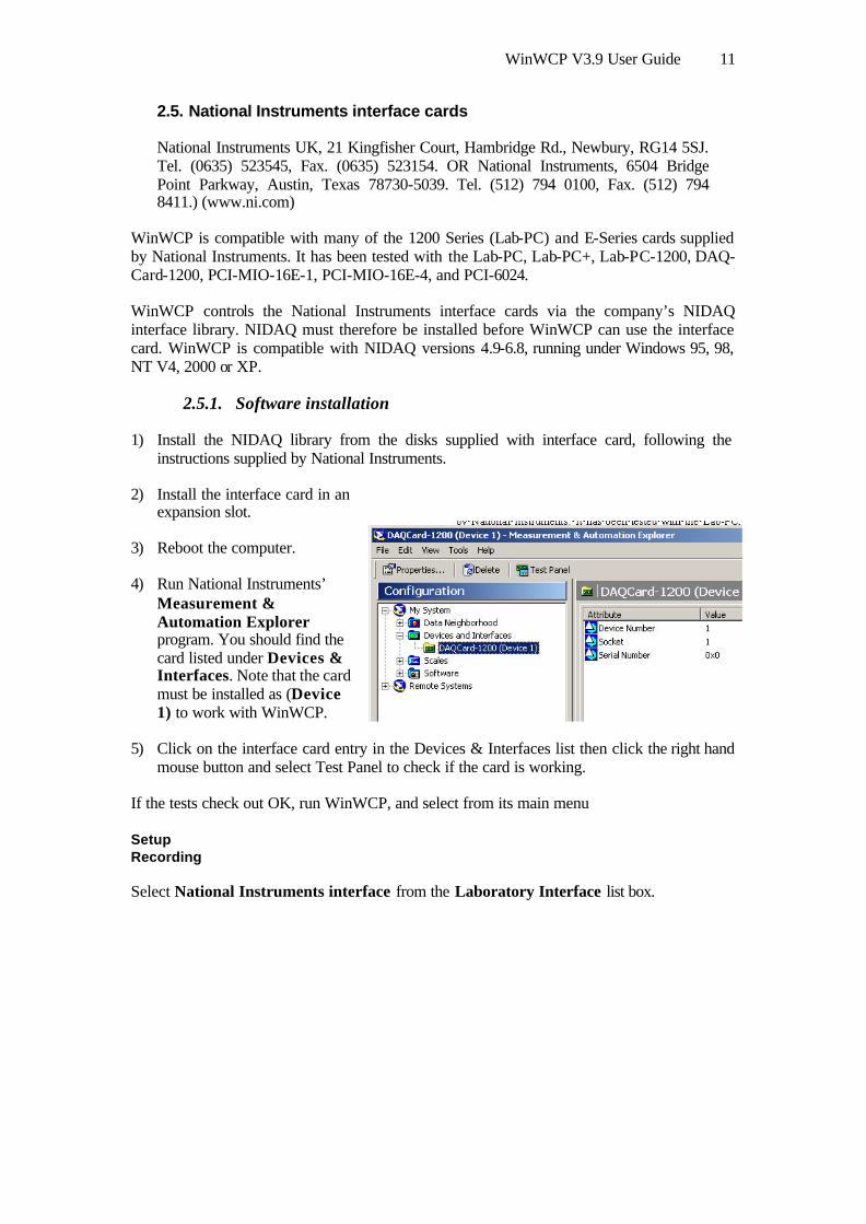
4) Run National Instruments’ Measurement & Automation Explorer program. You should find the card listed under Devices & Interfaces. Note that the card must be installed as (Device 1) to work with WinWCP.
5) Click on the interface card entry in the Devices & Interfaces list then click the right hand mouse button and select Test Panel to check if the card is working.
If the tests check out OK, run WinWCP, and select from its main menu Setup Recording Select National Instruments interface from the Laboratory Interface list box.

WinWCP V3.9 User Guide 12
2.5.2. Signal input / output connections Signal input and output from National Instruments cards are made via a 50 or 68 way ribbon cable connector on the rear of the card. A BNC socketed input/output panel (BNC-2090) is available from National Instruments for E-Series boards. Standard screw terminal panels with 50 way ribbon cable sockets can also be obtained from electronic component suppliers.
The input/output connections for 50 pin 1200- and 68 pin E-series boards are tabulated below. WinWCP channel 1200-Series (50 pin) E-Series (68 pin) Analogue inputs (s=signal,g=ground) (s=signal,g=ground) Ch. 0 ACH0 (s=1,g=9) ACH0 (s=68,g=67) Ch. 1 ACH1 (s=2,g=9) ACH1 (s=33,g=32) Ch. 2 ACH2 (s=3,g=9) ACH2 (s=65,g=64) Ch. 3 ACH3 (s=4,g=9) ACH3 (s=30,g=29) Ch. 4 ACH4 (s=5,g=9) ACH4 (s=28,g=27) Ch. 5 ACH5 (s=6,g=9) ACH5 (s=60,g=59) Ch.6 ACH6 (s=7,g=9) ACH6 (s=25,g=24) Ch.7 ACH7 (s=8,g=9) ACH7 (s=57,g=56) Analogue outputs Command voltage out DAC0 OUT (s=10,g=11) DAC0 OUT (s=22,g=55) Trigger/Sync. (See Note 1) Sync. pulse out (See Note 1)
DAC1 OUT (s=12,g=11) DAC1 OUT (s=21,g=54)
Recording Sweep External Trigger I/P (See Note 1)
EXTTRIG (s=38,g=50) PFI0/TRIG1 (s=11,g=44)
Stimulus Program External Trigger I/P (See Note 2)
PB0 (s=22, g=50) PFI1/TRIG2 (s=10, g=9)
Digital sync. in PC6 (s=36,g=50) - Digital Out Dig. 0 PA0 (s=14,g=13) - Dig. 1 PA1 (s=15,g=13) - Dig. 2 PA2 (s=16,g=13) - Dig. 3 PA3 (s=17,g=13) - Dig. 4 PA4 (s=18,g=13) - Dig. 5 PA5 (s=19,g=13) - Dig. 6 PA6 (s=20,g=13) - Dig. 7 PA7 (s=21,g=13) -
Note 1. Sync Pulse Out must be connected to Recording Sweep External Trigger I/P when recording signals using the Stimulus Program trigger mode and for the Seal Test option. For 1200 series boards only, Sync Pulse Out must also be connected to Digital Sync. In when the digital output pattern options (Dig 0 .. Dig 7) in the pulse protocol are in use.
Note 2. An active-high TTL pulse on this input triggers the start a stimulus program which has been set up with the External Stimulus Trigger = Y option. (1200 Series boards need the pulse to be 10 ms in duration or longer.)
WinWCP V3.9 User Guide 13
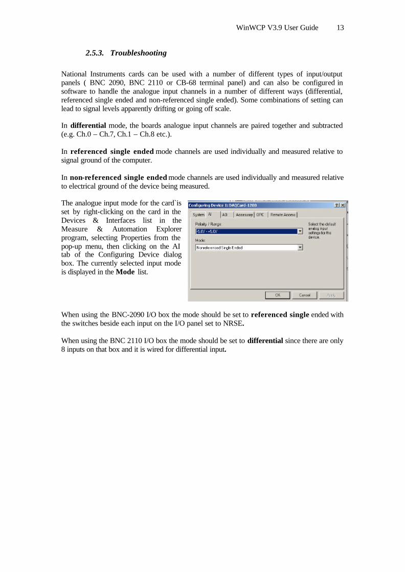
2.5.3. Troubleshooting National Instruments cards can be used with a number of different types of input/output panels ( BNC 2090, BNC 2110 or CB-68 terminal panel) and can also be configured in software to handle the analogue input channels in a number of different ways (differential, referenced single ended and non-referenced single ended). Some combinations of setting can lead to signal levels apparently drifting or going off scale. In differential mode, the boards analogue input channels are paired together and subtracted (e.g. Ch.0 – Ch.7, Ch.1 – Ch.8 etc.). In referenced single ended mode channels are used individually and measured relative to signal ground of the computer. In non-referenced single ended mode channels are used individually and measured relative to electrical ground of the device being measured. The analogue input mode for the card`is set by right-clicking on the card in the Devices & Interfaces list in the Measure & Automation Explorer program, selecting Properties from the pop-up menu, then clicking on the AI tab of the Configuring Device dialog box. The currently selected input mode is displayed in the Mode list. When using the BNC-2090 I/O box the mode should be set to referenced single ended with the switches beside each input on the I/O panel set to NRSE. When using the BNC 2110 I/O box the mode should be set to differential since there are only 8 inputs on that box and it is wired for differential input.

WinWCP V3.9 User Guide 14
2.6. Axon Instruments Digidata 1200
Axon Instruments Inc. 3280 Whipple Road, Union City CA 94587 U.S.A. Tel (510) 675-6200 (www.axon.com).
The Digidata 1200, 1200A and 1200B interface boards fully supports all WinWCP features.. They have a 330 kHz maximum sampling rates and 4 programmable input voltage ranges (±10V, ±5V, ±2.5V, ±1.25V). The Digidata 1200 is also supported by the pCLAMP electrophysiology software package. Inputs to and outputs from the board are via BNC connectors on an I/O box, connected to the board via a shielded ribbon cable.
In order to use WinWCP with a Digidata 1200, the following computer system resources must be available for use by the Digidata 1200.
• I/O port address 320-33F (Hex)
• DMA channels 5 and 6
WinWCP currently supports the Digidata 1200 under Windows 95 and 98 only. Windows NT and 2000 support is not available at present.
2.6.1. Software Installation
1) Install the Digidata 1200 card into an ISA computer expansion slot, and attach it to its BNC I/O panel using the shielded ribbon cable supplied with the card.
2) Click the Windows Start button and select Install Digidata 1200 driver (Win95/98) from within the WinWCP group in the Programs menu. Follow the instructions to install the Digidata 1200 Windows device driver. (WinWCP does not use the standard Axon Instruments Digidata 1200 device driver).
3) Reboot the computer.
4) Run WinWCP and select from its main menu Setup Recording Select Axon Instruments Digidata 1200 from the Laboratory Interface list box.

WinWCP V3.9 User Guide 15
2.6.2. Signal input / output connections Signal input and output connections are made via the BNC sockets on the front and rear of the Digidata 1200 I/O box.
WinWCP channel Name Analogue inputs Ch. 0 Analogue In 0 Ch. 1 Analogue In 1 Ch. 2 Analogue In 2 Ch. 3 Analogue In 3 Ch. 4 Analogue In 4 Ch. 5 Analogue In 5 Analogue outputs Command voltage out Analogue Out 0 Trigger/Sync. Sync. pulse out Analogue Out 1 See Note 1 Recording Sweep External Trigger I/P
Gate 3 (on rear) See Note 1
Stimulus Program External Trigger I/P
Digital Input 0 (on rear)
See Note 2
Digital sync. in - Digital Out See Note 3 Dig. 0 Digital Out 0 Dig. 1 Digital Out 1 Dig. 2 Digital Out 2 Dig. 3 Digital Out 3
Note 1. Sync Pulse Out must be connected to Recording Sweep External Trigger I/P when recording signals using the Stimulus Program trigger mode and for the Seal Test option.
Note 2. An active-high TTL pulse on this input triggers the start a stimulus program which has been set up with the External Stimulus Trigger = Y option. Note 3. The Digidata 1200 only supports 4 digital output lines.
2.6.3. Troubleshooting
There are two known problems which will prevent WinWCP from recording from a Digidata 1200’s analogue input channels.
I/O port conflict. The Digidata 1200 default I/O port addresses span the range 320H-33AH. These settings conflict with the default MIDI port setting (330H) of Creative Labs. Sound-Blaster 16 and similar sound cards. There are a number of solutions to this problem.
a) Change the Sound-Blaster MIDI port setting to a value higher than 33AH.
b) Remove the Sound-Blaster card (or disable it using the BIOS setup if it is built in to the computer motherboard).
DMA channel conflicts. WinWCP requires DMA channels 5 and 6 to support the transfer of data to/from PC memory and the Digidata 1200. Many sound cards also make use of DMA 5 and can interfere with the operation of the Digidata 1200.

WinWCP V3.9 User Guide 16
2.7. Axon Instruments Digidata 1320 Series
Axon Instruments Inc. 3280 Whipple Road, Union City CA 94587 U.S.A. Tel (510) 675-6200.
The Digidata 1320 Series (1320A, 1322) interfaces consist of self-contained, mains-powered digitiser units with BNC I/O sockets attached to the host computer via a SCSI (Small Computer Systems Interface) interface card and cable. A number of versions are available including the 1320A and 1322A. The 1322A supports sampling rates up to 500 kHz (16 bit resolution) on up to 16 channels. It has a fixed input and output voltage range of ±10V and supports 4 digital output channels. The Digidata 1320 Series is currently supported by WinWCP under Windows 95, 98, NT and 2000.
2.7.1. Software Installation WinWCP uses Axon’s standard software library (AxDD132x.DLL) for the Digidata 1320 Series. Details for steps (1)-(5) can be found in Axon’s Digidata 1320 Series Operator’s Manual.
1) Install the Axon SCSI card in a PCI expansion slot.
2) Attach the Digidata 1320 to the SCSI card and switch on the computer and 1320.
3) Install the AxoScope software supplied with the Digidata 1320.
4) Reboot the computer.
5) Run AxoScope to ensure that the software installed OK.
6) Run WinWCP and select from its main menu Setup Recording Select Axon Instruments Digidata 1320 from the Laboratory Interface list box.

WinWCP V3.9 User Guide 17
2.7.2. Signal input / output connections Signal input and output connections are made via the BNC sockets on the front of the Digidata 1320 Series digitiser unit.
WinWCP channel Name Analogue inputs Ch. 0 Analogue In 0 Ch. 1 Analogue In 1 Ch. 2 Analogue In 2 Ch. 3 Analogue In 3 Ch. 4 Analogue In 4 Ch. 5 Analogue In 5 Ch.6 Analogue In 6 Ch.7 Analogue In 7 Analogue outputs Command voltage out Analogue Out 0 Trigger/Sync. Sync. pulse out None Recording Sweep External Trigger I/P
Trigger In (Start)
Stimulus Program External Trigger I/P (See Note 1)
Trigger In (Start)
Digital Out (See Note 1) Dig. 0 Digital Out 0 Dig. 1 Digital Out 1 Dig. 2 Digital Out 2 Dig. 3 Digital Out 3
Note 1. The Digidata 1320 Series only supports 4 digital output lines.
Note 2. An active-high TTL pulse on this input triggers the start a stimulus program which has been set up with the External Stimulus Trigger = Y option. (1200 Series boards need the pulse to be 10 ms in duration or longer.)
2.7.3. Troubleshooting
When multiple analogue input channels are being sampled and the sampling interval is greater than 10 ms, samples get mixed up between channels. This problem can be seen to occur also with AxoScope, suggesting a bug in the Digidata 1320 firmware or AXDD132X.DDL library. The only limited solution at present is to increase the number of samples per record to ensure that the sampling interval is less than 10 ms.

WinWCP V3.9 User Guide 18
2.8. Instrutech ITC-16/18
The Instrutech ITC-16 and ITC-18 interfaces consist of self-contained, 19” rack-mountable, mains-powered digitiser unit with BNC I/O sockets attached to the host computer via a digital interface card and cable. Both the ITC-16 and ITC-18 support 8 analogue input channels, 4 analogue outputs (2 used by WinWCP) and 8 digital outputs. Both devices are currently supported by WinWCP under Windows 95, 98, NT and 2000. The ITC-16 and ITC-18 are manufactured by Instrutech Inc., 20 Vanderventer Ave., Suite 101E, Port Washington, New York 11050-3752 U.S.A. Telephone: (516) 883-1300. (www.instrutech.com)
2.8.1. Instrutech ITC-16/18 – I/O Panel Connections Signal input and output connections are made via the BNC sockets on the front of the ITC-16/18 unit.
WinWCP channel Name Analogue inputs Ch. 0 ADC Input 0 Ch. 1 ADC Input 1 Ch. 2 ADC Input 2 Ch. 3 ADC Input 3 Ch. 4 ADC Input 4 Ch. 5 ADC Input 5 Ch. 6 ADC Input 6 Ch. 7 ADC Input 7 Analogue outputs Command voltage out DAC Output 0 Sync. pulse out DAC Output 1 Trigger/Sync. Recording Sweep External Trigger I/P
Trig In
Stimulus Program External Trigger I/P (See Note 1)
Trig In
Digital Out Dig. 0 TTL Out 0 Dig. 1 TTL Out 1 Dig. 2 TTL: Out 2 Dig. 3 TTL Out 3
Note 1. An active-low TTL pulse on this input triggers the start a stimulus program which has been set up with the External Stimulus Trigger = Y option.

WinWCP V3.9 User Guide 19
2.8.2. Installing software support for the Instrutech ITC-16/18 WinWCP uses Instrutech’s device interface libraries for the ITC-16/18 family. Details for steps (1)-(3) can be found in the Instrutech Data Acquisition Interface user manual.
Installation Procedure
1) Install the Instrutech interface card in an expansion slot.
2) Attach the ITC-16 or ITC18 unit to the card.
3) Install the Instrutech Device Driver software supplied with the card (or downloaded from www.instrutech.com)
4) Reboot the computer.
5) Run the Instrutech test program installed with the device driver to test whether the software installed OK.
6) Run WinWCP and select from its main menu Setup Recording If you are using Instrutech's old device driver software (as supplied with the EPC-9 and downloadable from www.instrutech.com), select Instrutech ITC-16 (Old Driver) OR Instrutech ITC-18 (Old Driver) from the Laboratory Interface list box, depending upon which interface you have installed.
Note. Instrutech have also introduced a new software driver and library which supports the ITC-16, ITC-18 and ITC-1600. If you are using this library, select Instrutech ITC-16/18 (New driver) from the Laboratory Interface list box.
2.8.3. Instrutech ITC-16/18 : Troubleshooting WinWCP requires Instrutech's combined device driver library ITCMM.DLL (released late 2001). It may not work with earlier libraries.
WinWCP V3.9 User Guide 20
3. Using WCP - An Overview
WinWCP consists of a variety of program modules for recording and analysing electrophysiological signals. These modules are accessed via the main program menu on the program’s title bar and appear as independent sub-windows enclosed within the main WinWCP window.
The File menu provides the standard Windows functions for creating, opening and closing data file, printing and import and export to non-native data formats.
The Edit menu permits data to be copied to the Windows clipboard.
The View menu provides options for magnifying and selecting the type of record being displayed.
The Record menu invokes the digital recording module for recording analogue signals to disk and the seal test module for monitoring the sealing of patch pipettes to cells.
The Setup menu provides options for setting; the numbers of analogue channels to be recorded, recording sweep duration and other parameters; voltage-clamp command voltage stimulus patterns; and controlling external amplifiers.
The Analysis menu provides access to a range of analysis modules, which can be applied to the digitised signals stored on file. These include:
• A waveform analysis module for the automatic calculation of waveform parameters (peak and average amplitude, area, rise time, rate of rise, time to 50% and 90% decay, and variance). Results can be plotted as X/Y graphs or as histograms.
• A curve fitting module for fitting exponential and other curves to waveform transients.
• A signal averaging module.
• A leak subtraction module.
• A non-stationary variance analysis module
• A quantal content analysis module.
• A driving function analysis.
The Simulations menu provides access to modules for creating simulated end-plate currents and voltage-activated sodium currents.
The Windows menu selects between active windows.
The Help menu provides access to the WinWCP Help files.

WinWCP V3.9 User Guide 21
Ext Trig
Sync Out
Vcom Out
An. In Ch.0
An. In Ch.1
An. In Ch.2
Patch Clamp
4. Connecting WinWCP to your experiment
The first step in making a digital recording is to connect the signal outputs from your electrophysiological amplifier to the appropriate analogue inputs of the A/D converter in your laboratory interface unit. If you plan to use the computer to apply voltage pulse stimuli to the cell, you must also connect a D/A converter output to the command voltage input of the voltage-clamp. You may also have to supply a digital trigger pulse to initiate each recording sweep.
Depending upon the absolute levels produced by the recording device, you may need to amplify the signal to make it compatible with the input requirements of your A/D converters. You may also need to low-pass filter the signal and/or apply a DC offset to the signal, before it can be digitised. Two typical recording situations are discussed below.
4.1. Example 1 - Connecting WinWCP to a patch clamp.
One of the most common applications for WinWCP is recording from, and controlling, a whole-cell patch clamp experiment. Two analogue channels are normally recorded, membrane current and voltage, and computer-generated voltage pulses are applied to the patch clamp command voltage input to stimulate the cell. The patch clamp is connected to the computer as follows
Consult the signal connections table for your particular laboratory interface, in sections 2.4.2, 2.5.2 or 2.6.2, and make the following connections.
The membrane current (Im) output from the patch clamp is connected to WinWCP input channel Ch.0.
The membrane potential (Vm) is fed into WinWCP input channel Ch.1.
Voltage stimulus pulses generated at the WinWCP Command voltage output are passed to the Command voltage input (Vcom) of the patch clamp.
The patch clamp gain telegraph output is connected to WinWCP input channel Ch.2.
A synchronisation pulse is generated at the WinWCP Sync. pulse out and passed to WinWCP External trigger input so that recording sweeps can be synchronised with voltage pulse generation. Note. This connection is very important, otherwise stimulus pulse generation and the seal test functions will not work.
Vm
Im
Vcom
I/O Panel
Gain Telegraph

WinWCP V3.9 User Guide 22
Ext Trig
Sync Out
Vcom Out
An. In Ch.0
An. In Ch.1
4.2. Example 2 – Recording endplate potentials with WinWCP
The recording of endplate potentials (EPPs) from skeletal muscles (or EPSPs from neurons) presents an experimental situation where some signal conditioning may be required before digitisation. Intracellular EPPs are often no more than 5-10mV in amplitude and miniature EPPs only 1mV. Most recording devices such as the Axoclamp (Axon Instruments), or WPI 705 (World Precision Instruments) provide no more than X10 amplification, and sometimes only unity gain, at their voltage outputs. Typically, laboratory interface units are not sensitive enough to directly measure such small voltages.
Most of the laboratory interfaces supported by WinWCP are fitted with a 12 bit resolution A/D converter designed to digitise voltages within the range -5V to +5V. This means that, during digitisation, the A/D converter generates a 12 bit binary number proportional to the amplitude of the analogue voltage at its input. Twelve bits are sufficient to describe only 4096 discrete level. Thus, given a ±5V input range, the smallest voltage difference that can be directly measured is
100004096
2 44mVbits
mV bit= . /
Clearly, a 10mV amplitude EPP would be barely observable. Such small signals must be amplified to make them span a significant fraction of the input voltage of the A/D converter, e.g. 1-2V. Amplification factors in the order of 500-1000 are therefore required. Such high amplification factors require that the resting membrane potential is subtracted from the signal before amplification, to avoid overloading the A/D converter inputs. Although the EPP may only be 10mV in amplitude it is superimposed on a -90mV resting potential. Amplifying this signal by X500 would (theoretically) result in a signal with DC level of -45V. Most instrumentation amplifiers cannot sustain such a level, being limited to ±10V output levels. (In any case, signal levels exceeding 20V may damage the input stages of many A/D converter) The above difficulties can be overcome by using a differential amplifier as shown in the circuit below.
A differential amplifier has two inputs, (+) and (-), and amplifies the difference between them. The voltage output from the microelectrode amplifier is fed into the (+) input while a DC voltage level is fed into the (-) input, from a potentiometer. The resting membrane potential can thus be subtracted from the signal by adjusting the potentiometer. The signal is then amplified, low-pass filtered, and passed to analogue input channel 0 of the laboratory interface.
The low-pass filter is used to prevent the artefact of digital recording known as "aliasing" from occurring, by eliminating signal components at frequencies greater than half the A/D converter sampling frequency (known as the Nyquist frequency). Without such filtering, high
I/O Panel
Low -pass filter
Microelectrode amplifier
Differential amplifer
DC Offset
Stimulator
Sync. Out Stim Out
+
-

WinWCP V3.9 User Guide 23
frequency components appear falsely superimposed (aliased) on true lower frequencies. For example, if a signal is being sampled at a rate of 20kHz, the filter cut-off must be set no higher than 10kHz. Lower cut-off frequencies can be used, however, and act to smooth the signal.
The low-pass filter should be of a design which does not distort the signal time course, an 8 pole Bessel filter being a common choice. Further details on filtering and other aspects of signal conditioning can be found in Dempster (1993).
The circuit also shows a typical situation where a stimulator (such as a Grass S44) is being used to excite the nerve of a nerve-muscle preparation. Digital recording sweeps are synchronised with the stimulus pulses by connecting the "Sync. Out" output of the stimulator to the external trigger input of the laboratory interface. (Note. External trigger inputs are usually designed to be triggered by 5V digital TTL signals while older Grass stimulators produce 12V signals, so some form of signal level conversion may be necessary here also.)
Signal conditioning amplifiers and filters are available from a number of suppliers. Some examples include, the Frequency Devices 902LPF (a self-contained 8 pole Bessel low-pass filter with a differential amplifier input and gains of X1, X3.16 and X10) and. tbe Neurolog range of modular amplifiers and filters produced by Digitimer Ltd. Computer controllable signals conditioners are also now available such as the Axon Instruments CyberAmp and the CED 1902.

WinWCP V3.9 User Guide 24
5. Configuring WinWCP for a recording session
WinWCP digitises analogue signals from your experiments as series of discrete records, equivalent to oscilloscope sweeps, Up to 8 separate input channels can be acquired per record. Each record can hold up to a total of 29952 sample points.
Before making a digital recording for the first time, you must do the following :-
1) Create a data file to hold your recordings.
2) Define the number of analogue channels, number of samples per channel, etc. for the recording.
5.1. Creating a data file
To create a new data file to hold your recordings, select from the menu
File New
To get the New Data File dialog box, shown here.
Select the disk and folder into which the file is to be placed using the Save In list box. WinWCP data files have the extension extension ".wcp"
.
5.2. Setting recording parameters.
To set the number of channels to be recorded, recording
duration and other parameters select the option
Setup Recording Sweep
to display the Setup dialog box.
5.2.1. No. Channels Sets the number of analogue input channels you intend to record from. WinWCP supports a maximum of 8 channels. Channels are always acquired in sequence from Ch.0 upwards, i.e. No. Channels=1, selects Ch.0; No. Channels=2 selects Ch.0 & Ch.1 etc.

WinWCP V3.9 User Guide 25
5.2.2. Record Duration
Sets the default duration of each recording sweep. Set it to a value that is approximately 50% longer than the time course of the signals that you intend to record.
5.2.3. No. Samples/Channel
Sets the number of samples to be acquired per input channel within the recording sweep. The minimum is 256 samples per channel and increments are in units of 256. The maximum is 29952 / No. Channels. Note that the more samples acquired per record, the larger the size of the data files produced.
5.2.4. Sampling Interval
Displays the time between A/D samples acquired from each input channel. It is determined by the Record Duration and the No. Samples/Channel.
hannel Samples/CNo.Duration Record
Interval Sampling =
It is important to choose a sampling interval which is small enough to ensure that a sufficient number of samples are acquired during the most rapidly changing phases of the signals being recorded. For most types of signal, 1024 samples/channel and a record duration approximately 50% longer than the signal time course provide satisfactory results. (However, note that some signals, such as cardiac ventricular action potentials, can combine long time courses (200-300 ms) with very rapid rising phases (1-2 ms). In such circumstances, 8192 or more samples/channel might be required to accurately represent the rising phase.)
As discussed in section 4.2, to avoid aliasing artefacts, the analogue signals should be low-pass filtered to remove frequency components greater than half of the sampling rate (i.e. reciprocal of the sampling interval).
5.2.5. A/D Converter Voltage Range Defines the measurable voltage range of the A/D converter. The range of possible options depends upon the laboratory interface in use. The CED 1401, for instance, only has a single sensitivity ±5V, other interfaces such as the Axon Instruments Digidata 1200 have 4 programmable input sensitivities: ±10V, ±5V, ±2.5, and ±1.25V.
In order to get an accurate measure of the amplitude of an analogue signal it is important to ensure that it spans a significant proportion (30-50%) of the A/D converter's input voltage range. By changing the voltage range you can adapt the sensitivity of the A/D converter to best match the amplitude of the signals from your experiment.
5.2.6. Time Units
Determines whether time measurements are presented in units of seconds or milliseconds.

WinWCP V3.9 User Guide 26
5.2.7. Channel Calibration Table WinWCP can display the signals stored in each input channel in the units appropriate to each channel. In order to do this correctly, the names, units and scaling information for each channel must be entered into the Channel Calibration Table . There are 3 entries in the table for each analogue channel.
Names contains a 1-4 letter name used to identify the source of the channel (e.g. Vm, Im).
Units defines the measurement units of the signal (e.g. mV, pA etc.).
V/Units defines the scaling factors relating the voltage level at the inputs of the A/D converter (in V) to the actual signal levels in each channel (in the channel units).
For instance, if the membrane voltage output of your patch clamp supplies a signal which is 10X the measured membrane potential of the cell, and the units have been defined as mV, then the appropriate V/Units setting is 0.01 (since the patch clamp voltage output is 0.01 Volts per mV)
In the case of patch clamp current channels, the V/Units value is determined by the current gain setting which is usually a switchable value, e.g. if the current output was set at 20 mV/pA, and the channel units were pA, the V/Units settings would be 0.02.)
A typical setup for a patch-clamp experiment, recording current and voltage channels is shown below. Current is recorded in channel 0, which is named Im, and has units of pA.
Name V/Units Units Ch.0 Im 0.02 pA Ch.1 Vm 0.01 mV
5.2.8. Amplifiers WinWCP can automatically determine the current gain factor for a number of patch clamp amplifiers and use it as the calibration factor for input channel Ch.0. To enable this facility, 1) Select your amplifier from the Amplifiers list. (Axon Axopatch 1D and 200 are current
supported.)
2) Connect an unused input channel to the Gain Telegraph output of the patch clamp, and enter the number of that channel in the Telegraph Ch. Box.
3) Enter the minimum gain setting of the patch clamp in the V/Units box for Ch.0.
If a CED 1902 computer-controllable amplifier is in use, this option can also be used to read its gain setting. (No Telegraph Ch. is required in this case.)

WinWCP V3.9 User Guide 27
6. Monitoring input signals & patch pipette seal test
After a data file has been created and input channel parameters defined, you can monitor the signals appearing on each channel using the signal monitor/pipette seal test module. This module provides a real-time oscilloscope display and digital readout of the signal levels on the cell membrane current and voltage channels. A test pulse can also be generated for monitoring pipette resistance in patch clamp experiments.
To open the monitor/seal test module, select from the menu
Record Monitor/Pipette Seal Test
An oscilloscope trace showing the current signal on each input channel is displayed.
6.1. Select current and voltage channels
Select the input channels, which contain the current and voltage signals, by selecting the current channel in the current list.
and the voltage channel in the voltage list
6.2. Command voltage divide factor
Most voltage and patch clamp amplifiers divide down their command voltage input signals by some factor in the range 10-50. Enter the scaling factor into the Vcom divide factor box. WinWCP uses this factor to scale the stimulus voltage output to the D/A converter to obtain the correct voltage at the cell. (Note. Axon Instruments amplifiers require a divide factor of 50 while the Heka EPC-7 patch clamp requires a divide factor 10.)
6.3. Cell holding voltage and test pulses
You can control the holding voltage applied to the cell and the amplitude and duration of a test voltage pulse by selecting one of two available test pulse types (Pulse #1, Pulse #2) or a holding voltage level without a pulse (Pulse #3).
The size of each pulse type is set by entering an appropriate value for holding voltage and pulse amplitude into the Holding voltage or Amplitude box for each pulse.
The width of both pulses is defined by the pulse width box
You can switch between pulses by pressing the function key associated with each pulse (Pulse #1 = F3, Pulse #1 = F4, Pulse #1 = F5).

WinWCP V3.9 User Guide 28
6.4. Current and voltage readouts
A readout of the cell membrane holding current and voltage, and test pulse amplitude, appears at the bottom of the monitor window.
During initial formation of a giga-seal, the Pipette option displays pipette resistance, computed from
pulse
pulsepipette I
VR =
where Vpulse and Ipulse are the steady-state voltage and current pulse amplitudes. The Cell option displays the cell membrane conductance, Gm, capacity, Cm, and access conductance, Ga, computed from
( )mam
a
pulsepulse
pulsem
pulsea
GGC
GI
V
IG
VI
G
+=
−
=
=
τ
0
where I0 is the initial current at the peak of the capacity transient and τ is the exponential time constant of decay of the capacitance current (See Gillis, 1995, for details). Note. If Ga, Gm and Cm are to be estimated correctly, the patch clamp’s pipette series resistance compensation and capacity current cancellation features must be turned off.
A good test, to check if WinWCP is set up with the correct input/output connections and channel scaling factors, is to attach the model cell supplied with most voltage/patch clamps, and observe the holding potential and current, test pulse amplitude and cell parameters correspond with the known values of the model.
6.5. Display scaling and sweep triggering
The vertical display magnification is automatically adjusted to maintain a visible image of the test pulse within the display area. The magnification factor in current use is indicated in the Display box.
Automatic scaling can be disabled by selecting the Manual option. A fixed display magnification can then be entered in the box.
Note. The laboratory interface Sync. Pulse output must be connected to the External Trigger Input for test pulses and monitor sweeps to be generated (see section 4.1). If you wish to monitor input signals without generating test pulses, check the Free run check box, allowing sweeps to occur without the Sync. Pulse – External Trigger connection.

WinWCP V3.9 User Guide 29
7. Making a recording
After a data file has been created, and an appropriate set of recording parameters defined, select
Record Record to disk
to enter the recording module. The display area of the screen acts like a digital oscilloscope, showing traces of the signals as they are recorded. To collect a series of records: 1) Enter a line of text identifying the purpose of the recording in the Ident box (optional).
2) Enter the number of records to be collected in the Records Required box.
3) Set the trigger mode (see below for details)
4) Make sure that the Save to File box is checked. 5) Start recording, by clicking the Record button
6) If you want to stop recording before the number of records in the Records Required box
have been collected, click the Stop button.

WinWCP V3.9 User Guide 30
7.1. Trigger modes
In general, recording sweep(s) must be synchronised with the start of the signals under study, to ensure that the signal is captured within the record and always appears in the same place. The trigger mode determines how this synchronisation takes place.
There are 4 modes
• Free Run • External Trigger • Event Detector • Stimulus Program
You must select a trigger mode appropriate to the type of signal to be recorded and the configuration of your recording system.
7.1.1. Free Run The Free Run trigger mode is used for unsynchronised recording. Recording sweeps start immediately after the Record button is pressed and continue until the required number of records have been collected.
Choose the free run mode for simple tests of the laboratory interface and for signals, such random ion channel noise, where synchronisation is not possible or required.
7.1.2. External Trigger
Many kinds of electrophysiological signals are evoked by stimulating the cell or tissue, using an electrical stimulator. In order to record such signals, the recording sweep must be synchronised with the stimulator, ideally so that the sweeps starts shortly before the cell is stimulated. The External Trigger mode links the start of recording sweeps to a trigger pulse applied to the Ext. Trigger input of the laboratory interface.
Choose the External Trigger mode when you are using a stimulator to evoke the signals under study. Note. the "Sync. Pulse" output of the stimulator must be connected to the external trigger input of the laboratory interface for triggering to occur. During a stimulus cycle, the sync. pulse is produced first (triggering the recording sweep) and, after a delay (settable on the stimulator front panel), the stimulus itself.
7.1.3. Event Detector
The event detector mode provides a means of detecting signals as they occur within an incoming analogue signal. A threshold-based event detection algorithm monitors the incoming signal on one of the input channels. An event is detected when the signal deviates by more than a predetermined level from the average baseline level. To compensate for slow drifts in the baseline level, the threshold level is maintained at a constant distance from the baseline by means of a running average calculation. The event detector is configured by setting three parameters.
If more than one channel is being recorded, select the input channel on which events are to be detected from the detection Ch. list box.
Enter the detection threshold into the Threshold box. The threshold level is expressed as a percentage of the total input range, with its polarity determining whether positive- or negative-going signals are to be detected. The level should be set as small as possible to maximise the likelihood of an event being detected, but without producing an excessive number of false

WinWCP V3.9 User Guide 31
events due to background noise triggering the detector. Values of around 5-10% are often used, but several trials may be necessary before the best level for a particular experiment is found.
The Pretrigger setting determines the percentage of the record to be collected before the detection point. A typical value is 30%.
7.1.4. Stimulus Program
In Stimulus Program mode, WinWCP functions as a stimulator as well as a recording device. Sequences of recording sweeps are acquired at timed intervals, in synchrony with computer-generated stimuli applied to the cell. The stimuli can be in the form of either command voltage waveforms or digital pulses for controlling valves or other devices.
Choose Stimulus Program mode when there is a need to apply a sequence of voltage pulses in order to stimulate voltage-activated ionic currents in cells, or apply other complex stimulus patterns.
Each stimulus pulse is associated with a single recording sweep and the duration or amplitude of any part of a pulse can be incremented between records. A complete stimulus protocol thus consists of a series of one or more pulses, incremented in amplitude or duration to create a family of pulses. Complex stimulus waveforms can be produced, including series of rectangular steps, ramps, and digitised analogue signals. Protocols are created using the Stimulus Generator module and stored as protocol files.
A list of available protocols appears in the Stimulus Program list box, allowing quick selection of protocols during a recording session.

WinWCP V3.9 User Guide 32
8. Creating stimulus protocols
To create a stimulus protocol file, select
Setup Stimulus Protocol Editor
to open the stimulus editor module. A diagram of the waveform appears in the Waveform display box. The voltage waveform is shown at the top (Vcom) with digital pulse patterns (if in use) below. The duration of the recording sweep is shown as a red bar.
Click the New button to create a blank protocol.
8.1. Building a stimulus protocol
The first stage in building a stimulus protocol is to define the number, duration and timing of the recording sweeps to be contained in the protocol. To set these parameters, click on the icon
to display the recording sweep parameters table.
The interval between recording sweeps entry sets the time interval between successive recording sweeps within the protocol.
The duration of recording sweep entry sets the duration of the sweep. (Note. Sweep duration must be at least 200 msec shorter than the interval between sweeps to allow time for records to be written to the data file.)
The number of repetitions of each waveform entry sets the number of times that a sweep is to be repeated with the same stimulus waveform.
The delay before start of recording entry allows the start of the recording sweep to be delayed relative to the start of waveform generation.
The delay increment entry increments the above delay between records.
The holding voltage entry sets the holding voltage to be used between waveform sweeps during the execution of a protocol. (This value overrides the default holding voltage set in the Seal Test module and Default Settings options).
The External Stimulus trigger (Y/N) entry allows the stimulus program to be triggered by an external TTL pulse instead of the internal timer. When set to Y, the Interval between sweeps entry is ignored and the stimulus program begins when a TTL pulse is received on the External Stimulus Trigger Input (See interface card connections tables in section 1.)

WinWCP V3.9 User Guide 33
8.2. Creating a voltage stimulus waveform
Waveforms are constructed by dragging waveform elements from the Toolbox and dropping them into the Voltage Command list.
A single voltage waveform can consist of up 10 separate elements. The amplitude and duration for each element is defined in its parameters table which can be made to appear by clicking the element. An element can be one of 6 types :
8.2.1. Rectangular voltage pulse of fixed size
This is a simple pulse, which does not vary in amplitude and duration between records. It has 3 parameters.
• Initial Delay defines the delay period before the pulse begins.
• Amplitude defines the pulse amplitude (mV).
• Duration defines the duration of the pulse.
This element can be used to provide series of stimuli of fixed size or, in combination with other elements, to provide fixed pre-conditioning pulses.
8.2.2. Family of rectangular pulses varying in amplitude
This is a rectangular voltage pulse whose amplitude is automatically incremented between recording sweeps. It has 5 parameters.
• Initial delay defines the delay period before the pulse begins.
• Start at Amplitude defines the amplitude of the first pulse in the protocol sequence.
• Increment by defines the increment to be added to the pulse amplitude between records.
• Number of increments defines the number of steps in the sequence.
• Pulse duration determines the duration of the pulse.
This element is typically used to explore the voltage-sensitivity of ionic conductances, by generating records containing the whole -cell membrane currents evoked in response to a series of voltage steps to different membrane potentials.

WinWCP V3.9 User Guide 34
8.2.3. Family of rectangular voltage pulses varying in duration
This is a rectangular voltage pulse whose duration can be automatically incremented between recording sweeps. It has 5 parameters.
• Initial delay defines the delay period before the pulse begins.
• Amplitude defines the amplitude of the pulse.
• Pulse duration determines the duration of the pulse.
• Increment by defines the increment to be added to the pulse duration between records.
• Number of increments defines the number of steps in the sequence.
This element is most commonly used as a variable duration preconditioning pulse in 2 or 3 step protocols for investigating inactivation kinetics of Hodgkin-Huxley type conductances.
8.2.4. Series of rectangular voltage pulses
This is a train of rectangular voltage pulses of fixed size. It is defined by 5 parameters
• Initial delay defines the delay period before the series of pulses begin.
• Amplitude defines the amplitude of each pulse in the series.
• Duration defines the duration of each pulse.
• Pulse interval (within train) determines the time interval between pulses.
• Number of pulses defines the number of pulses in the series.
This element can be used to produce a series of stimuli to observe the effect of repeated application of a stimulus at a high rate. It can also be used to produce a train of pre-conditioning stimuli if the delay and duration of the recording sweep is adjusted to acquire only the last pulse in the series (or a subsequent test pulse defined by another element).
8.2.5. Voltage ramp
This element produces a linear voltage ramp between two voltage levels. It is defined by 4 parameters
• Initial delay defines the delay period before the series of pulses begin.
• Start at amplitude defines the voltage level at the start of the ramp.
• End at amplitude defines the voltage level at the end of the ramp.
• Ramp duration defines the time taken for the voltage to slew between the start and end amplitudes.
Voltage ramps provide a means of rapidly generating the steady state current-voltage relationship for an ionic conductance. (Note that, the ramp generated by the computer is not truly linear, but consists of a staircase of fine steps. These steps can be smoothed out, by low-

WinWCP V3.9 User Guide 35
pass filtering the voltage stimulus signal before it is fed into the patch clamp.)
8.2.6. Digitised analogue waveform
Digitised analogue waveforms which have been previously acquired by WinWCP (or synthesised by another program) can be used as a waveform element.
To insert a digitised waveform into the protocol:
1) Select the source of the waveform and copy it to the Windows clipboard. Waveforms may be copied from a WinWCP signal record (using the Edit/Copy Data menu option) or from a spreadsheet or similar program.
2) Drag a digitised analogue waveform icon from the toolbox and drop it into the protocol list.
3) Insert the waveform into the protocol by clicking the
button. The waveform appears in the waveform display and its data points appear in the parameters table.
The parameters table consists of:
• Initial delay defines the delay period before the series of pulses begin.
• A list of data points for the analogue waveform. The waveform can be altered by modifying this list.
There are a number of limitations when using the digitised waveform element.
a) Only one digitised waveform element is permitted per protocol.
b) Digitised waveforms must consist of less than 1000 data points.
c) The sampling interval of the digitised waveform must be greater than 0.1 msec.
d) If digitised waveforms are created with a spreadsheet, the data points must be formatted as a pair of columns containing time (msecs) in the first and amplitude (mV) in the second. E.g. T0 V0 T1 V1 …etc
8.3. Creating a digital stimulus pattern
Digital stimulus patterns control up to 8 digital output lines (Dig.0 – Dig.7), if these are supported by the laboratory interface. Digital stimuli can be controlled simultaneously with the voltage stimulus.
To create a digital stimulus pattern, drag a digital stimulus element from the Toolbox and drop it into the digital pattern list.

WinWCP V3.9 User Guide 36
Each entry in the list controls one digital output, with the left-most entry controlling Dig.0 and the right-most Dig.7. Each of the 8 outputs can thus have a pattern which is executed simultaneously during the protocol (unlike the voltage waveform where elements are executed sequentially).
There are 3 digital stimulus elements.
8.3.1. Digital pulse (fixed duration)
This produced a digital pulse on the selected output line of fixed duration. It is defined by 4 parameters.
• Initial delay defines the delay before the start of the pulse.
• Increment delay by defines the amount that the delay is incremented by between recording sweeps.
• Duration defines the duration of the digital pulse.
• Invert Signal defines whether the digital pulse is an OFF-ON or an ON-OFF pulse. If set to No, the digital line is initially OFF (0V) and switches to ON (5V) during the pulse. If set to Yes, the digital line is initially ON (5V) and switches to OFF (0V) during the pulse.
The digital pulse element can be used to switch open or close valves controlling the flow of solutions over a cell. Multiple digital outputs can be used to simultaneously open one valve while another is closed.
8.3.2. Family of digital pulse (varying in duration)
This produced a digital pulse on the selected output line, with a duration which is incrementable between records. It is defined by 5 parameters.
• Initial delay defines the delay before the start of the pulse.
• Starting duration defines the duration of the first pulse in the protocol.
• Increment by defines the amount that the duration is incremented between records.
• Number of increments defines the number of increments in the protocol. (Note that, if there are any voltage waveform elements in use within the protocol, the number of increments defined here must be the same.)
• Invert Signal defines whether the digital pulse is an OFF-ON or an ON-OFF pulse. If set to No, the digital line is initially OFF (0V) and switches to ON (5V) during the pulse. If set to Yes, the digital line is initially ON (5V) and switches to OFF (0V) during the pulse.

WinWCP V3.9 User Guide 37
8.3.3. Train of digital pulses
This produces a series of digital pulses of fixed intervals and of fixed duration. It is defined by 5 parameters.
• Initial delay defines the delay before the start of the first pulse in the series.
• Pulse duration defines the duration of the each pulse in the series.
• Inter-pulse interval defines the time interval between pulses in the series.
• Number of pulses defines the number of pulses in the series.
• Invert Signal defines whether the digital pulse is an OFF-ON or an ON-OFF pulse. If set to No, the digital line is initially OFF (0V) and switches to ON (5V) during the pulse. If set to Yes, the digital line is initially ON (5V) and switches to OFF (0V) during the pulse.
This element can be used to apply a rapid train of stimuli to a cell.
8.4. Command voltage divide factor
Most voltage and patch clamp amplifiers divide down their command voltage input signals by some factor. Enter the scaling factor into the command voltage divide factor box. WinWCP uses this factor to scale the stimulus voltage output to the D/A converter to obtain the correct voltage at the cell. Axon Instruments amplifiers require a divide factor of 50 while the Heka EPC-7 patch clamp requires a divide factor of 10.
8.5. Recording Sweep Trigger Pulse
Trigger Pulse Sets the polarity of the trigger pulse used to synchronise the start of a recording sweep with a stimulus protocol and seal test pulses. This trigger pulse is produced on D/A output channel 1 (DAC1). When Trigger Pulse is set to Normal, a 1 msec, active-low pulse TTL is produced (i.e. the DAC1 output is at 5V and drops to 0V for 1 msec to trigger the recording sweep). When Trigger Pulse is set to Inverted a 1 msec active-high pulse is produced.
NOTE. The Inverted Trigger Pulse option is provided to allow the DAC1 output to be used to synchronise external devices (e.g. stimulators) which require an active-high TTL trigger pulse with the start of the recording sweep. Otherwise the setting should not be changed from Normal. It should be noted that a stimulus protocol with TTL digital pattern outputs will only work with the Normal trigger pulse setting when using CED 1401 series interfaces.
8.6. Leak subtraction
A protocol can be programmed to add digital leak subtraction records by selecting the P/N mode option. When this option is set, a series of additional sweeps are generated for each record defined in the protocol, using an inverted and scaled down version of the command voltage waveform. A digital average is obtained from these records and stored as a “LEAK” record, along with the basic “TEST” record.

WinWCP V3.9 User Guide 38
You can change the number of pulses used to compute the “LEAK” record and division factor by altering the values in the boxes shown. The default values are 4 leak records with voltage waveform divided by –4.
Note that subtraction of the “LEAK” from “TEST” records is done using the leak subtraction module. (See section 13 for details.)
8.7. Protocol linking
Recording normally stops when the requested sequence of records within a protocol is completed. Protocols can, however, be linked together by selecting a protocol from the Link to next protocol list, so that on completion of the first protocol, control is transferred to the linked protocol.
8.8. Saving and loading stimulus protocols
When you have created a stimulus protocol, you can save it to a protocol file by clicking the Save As button to get the Save Stimulus Protocol dialog box.
Stimulus protocols are stored as files with .VPR file extensions, in the directory, C:\ \WinWCP\vprot\
Protocol files can be re-loaded into the Stimulus Generator for editing, by clicking the Open
button, and selecting a protocol file from the list presented in the Load Stimulus Protocol dialog box.
8.9. Stimulus protocol examples
A number of example protocols are installed in the vprot folder when WinWCP is installed.
Steps.vpr A family of 12 depolarising, 500 msec duration, voltage steps, ranging
from 10 mV to 120 mV.
TailCur.vpr A family of 2-step pulse protocol for recording tail currents. A 500 msec pre-pulse, followed by a 60 mV, 50 msec duration test pulse. The pre-pulse steps from 10mV to 120 mV. The recording sweep is of 70 msec duration and begins 10 msec before the test pulse.
Ramp.vpr A voltage ramp, slewing from –100 mV to +100 mV over a period of 1 sec.
Ap.vpr A digitised action potential waveform.
Digpulse A digital stimulus program controlling digital outputs 0 and 1. Dig.0 is OFF initially and pulses ON for a period of 50 msec, after a delay of 100 msec. Dig. 0 is ON initially and pulses OFF for 50 msec.

WinWCP V3.9 User Guide 39
9. Viewing digitised records stored on file.
To view signal records stored in a data file, select from the menu.
View Raw records
to open the record display module.
Each record in the file can be displayed and measurements made of the signal levels within each channel using a movable cursor. The displayed record (or superimposed groups of records) can be printed out. Records can be assessed for the presence of interference other artefacts and marked as rejected, or assigned with particular record types.
9.1. Selecting and displaying records
Each record in the data file is numbered in the sequence that it was recorded. Records can be selected for display using the selection bar to move back or forward through the file. You can jump directly to a record by entering its number into the record number box above the selection bar. (You can also use the Ctrl+Plus and Ctrl+Minus keys to step forward or backwards through the file.)
To superimpose (up to 200) records on the display, select
View Auto Erase
to disable automatic display erasure when records are. (Selecting the option again re-enables auto-erase.)
9.2. Magnifying the display
To adjust the display magnification, select the channel to be changed by double -clicking on the signal trace.
The selected channel is expanded to fill the display window and the message “Zoom In/Out” appears at the top-left, indicating that the display is in zoom mode.
A rectangular box defining the currently selected upper and lower display limits is superimposed on the signal. Drag the edges of this box to indicate the new region of the record to be displayed. Then double-click again to return to normal display mode at the new magnification setting.
You can set all channels back to minimum magnification by selecting
View Zoom Out (All)
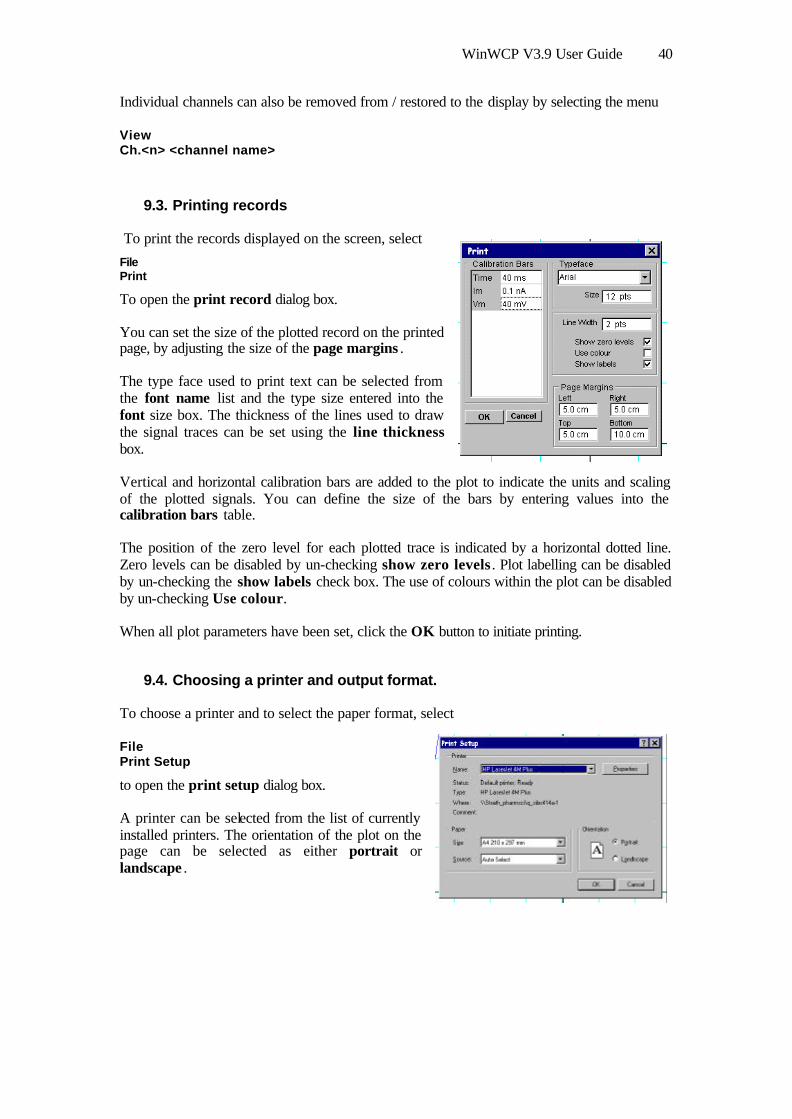
WinWCP V3.9 User Guide 40
Individual channels can also be removed from / restored to the display by selecting the menu
View Ch.<n> <channel name>
9.3. Printing records
To print the records displayed on the screen, select
File Print
To open the print record dialog box.
You can set the size of the plotted record on the printed page, by adjusting the size of the page margins .
The type face used to print text can be selected from the font name list and the type size entered into the font size box. The thickness of the lines used to draw the signal traces can be set using the line thickness box.
Vertical and horizontal calibration bars are added to the plot to indicate the units and scaling of the plotted signals. You can define the size of the bars by entering values into the calibration bars table.
The position of the zero level for each plotted trace is indicated by a horizontal dotted line. Zero levels can be disabled by un-checking show zero levels . Plot labelling can be disabled by un-checking the show labels check box. The use of colours within the plot can be disabled by un-checking Use colour.
When all plot parameters have been set, click the OK button to initiate printing.
9.4. Choosing a printer and output format.
To choose a printer and to select the paper format, select
File Print Setup
to open the print setup dialog box.
A printer can be selected from the list of currently installed printers. The orientation of the plot on the page can be selected as either portrait or landscape .

WinWCP V3.9 User Guide 41
9.5. Rejecting flawed records
Digitised records cannot all be assumed to be perfect. Consequently, the visual inspection of records, and the elimination of flawed records, is an important part of the analysis process. If automated waveform measurement procedures are to be applied, a mechanism is required for excluding flawed records from the analysis.
Checking a record’s rejected box marks a record as being flawed. Rejected records are excluded from automatic waveform, curve fitting, signal average or leak subtraction calculations. (Note. Pressing the Ctrl+R key combination is a quick way of toggling the rejected check box on and off.)
9.6. Classifying records
Records can also be classified according to the type of signal that they contain, by selecting a type from the record’s type list box. Eight types of records are currently defined (TEST, LEAK, EVOK, MINI, FAIL, TYP1, TYP2, TYP3).
The EVOK, MINI and FAIL types are used in the quantal analysis of synaptic currents or potentials (see section 15) to indicate whether a record is a nerve-evoked, spontaneous, or a nerve-evoked/transmission failure event. (Note. Types can be selected quickly using the Ctrl+T, Ctrl+L, Ctrl+E Ctrl+M, Ctrl+F keys.)
TEST and LEAK are used in the digital leak subtraction process (see section 13), and used to distinguish, respectively, normal records, containing voltage-activated currents, and records containing leak currents to be scaled and subtracted from the TEST records.
TYP1, TYP2 and TYP3 are general-purpose, user-defined record types.
9.7. Cursor measurement of signal levels
To measure the signal at any point on the displayed record, use the mouse to drag the vertical readout cursor to the desired part of the trace. Fine positioning of the cursor can be achieved by pressing the ← or → arrow keys with the mouse pointer over the selected cursor. The signal level of the trace(s) at the cursor position is displayed at the bottom of the window, below the cursor. Time measurements are made relative to the start of each record and (in brackets) relative to the location of the t=0 cursor. Signal levels are measured relative to each channel’s horizontal zero level cursor.
Cursor measurements can be written to the WinWCP log file by clicking the Save (F1) button. The Centre Cursor button places the readout cursor to the centre of the displayed region.

WinWCP V3.9 User Guide 42
9.8. Zero levels
The signal zero level for a channel can be defined in either of two ways. In From record mode, it is computed as the average level from a defined portion of each record. In Fixed mode, it is fixed at a level defined by the user and does not vary from record to record.
9.8.1. From record mode
If you want to compute the zero level from a portion of the signal record itself:
a) Move the mouse pointer over the horizontal zero level cursor of the channel you want to change. (The mouse pointer turns into an up/down arrow.)
b) Slide the mouse pointer horizontally until it overlies the region of the record which is to be defined as the zero level.
c) Click the right-hand mouse button to open the zero level dialog box.
d) Select the From Record option.
e) The zero level is computed, for each record, from the average of a series of (default=20) samples starting at the sample indicated in the At sample box. If you want to change the number of samples averaged to compute the zero level, change the value in the No. averaged box.
f) Click the OK button to use the new zero level.
Choose the from record mode when you want to measure transient signals, which are superimposed upon a baseline level which may be varying from record to record. Synaptic currents such as endplate currents or excitatory postsynaptic currents in neurons typically fall into this category.
9.8.2. Fixed mode If you want fix the zero level at a constant value to be used for all records in the file:
a) Move the mouse pointer over the horizontal zero level cursor of the channel you want to change. (The mouse pointer turns into an up/down arrow.)
b) Hold down the left mouse button and drag the zero level cursor vertically until it is at the desired level.
c) Click the right- mouse button to open the zero level dialog box.
d) Select the Fixed option. The vertical position of the fixed baseline is indicated (in A/D converter units) in the Level box. You can set the zero level by entering a value.
e) Click the OK button to use the new zero level.
Choose the fixed mode when you want to make measurements relative to a fixed absolute level. Fixed mode is typically used for the membrane potential measurements in voltage/patch clamp studies of voltage-activated current. (Note . Entering a value of zero into the Level box sets the zero level to the true zero voltage level for the channel)

WinWCP V3.9 User Guide 43
9.9. Copying records to the Windows clipboard
The displayed signal record(s) can be copied to the Windows clipboard in a variety of formats – a data table, an image, a WinWCP data record.
9.9.1. Copying data values Each signal record consists of an array of A/D converter sample values. A table of data values for the active display record can be copied to the clipboard by selecting
Edit Copy Data
The data is placed on the clipboard as a table, containing the scaled values for each sample in the record, in the measurement units defined for each channel. The table is stored in tab text format, allowing the data to be copied into programs such as spreadsheets and graph plotting packages, using an Edit/Paste command. (Note that due to limitations in the capacity of the Windows clipboard data points may be skipped to keep the size of the copied record within clipboard storage limits.)
9.9.2. Copying the displayed image.
The signal record(s) on the display can be copied to the clipboard as a bit mapped image by selecting
Edit Copy Image
to open the copy image dialog box.
The dimensions of the bit map, which will hold the image, can be set using the width and height image size boxes. The more pixels used in the bit map the better the quality of the image. Calibration bars, zero levels and text font, size and line thickness can be set in the same way as for a printed image.
When the image parameters have been set, click the
OK
button to copy the image to the clipboard.
9.10. Smoothing the displayed records
A digital low-pass filter algorithm can be used to smooth the displayed signal. To enable to filter, select a cut-off frequency from the Low pass filter list.
The low pass filter set in the display module also acts upon the records in waveform measurement, curve fitting and other modules. (Note that the record on the data file is preserved, filtering takes place when the record is read from the file.)

WinWCP V3.9 User Guide 44
10. Automatic measurement of signal waveforms
The automatic waveform measurement module provides a means of automatically making series of standard measurements on the digitised signals. Ten basic amplitude and duration measurements can be made on each channel and stored with each record. The results for each record are displayed on screen. In addition, sets of measurement variables can be plotted against each other, or compiled into histograms. A summary report showing mean value and standard errors for the measurement sets can also be produced.
10.1. Preparation for waveform analysis
If the results of an automated measurement procedure are to have meaning it is essential to ensure that the data supplied in the signal records are of good quality, i.e. free of artefacts or other imperfections. Each record in the data file to be analysed should therefore be visually inspected, using the record display module (see section 9) and rejected if it contains an artefact. This is a time consuming, but essential, process.
10.2. Making waveform measurements
After the records in the data file have been validated, select
Analysis Measure Waveforms
to open the waveform measurement module
The module is split five functional sections (pages) accessed by clicking on the page tab.
The Analysis page is used to set up the parameters of the waveform analysis and initiate the automatic measurement sequence, which generates a table of measurements.
The X/Y plot page is used to create X-Y graphs of the measurements.
The Histogram page is used to create frequency histograms of measurement.
The Summary page presents a summary (mean, standard deviation, etc.) of the measurements for the series of records analysed.
The Tables page is used to create tables of results.
10.3. Running a waveform analysis sequence
The first stage in the measurement process is to define and run a waveform analysis sequence on a selected series of records.
1) Select the Analysis page by clicking on its page tab.
2) Define the range of records to be analysed, by selecting All Records to analyse all records, or This Record to analyses only the currently displayed record, or Range and enter a range of records.
3) Select the type of records to be measured by selecting an option from the Type list. Select ALL to measure records of any type (except rejected records).

WinWCP V3.9 User Guide 45
4) Set the peak finding mode . Select absolute to define the peak value as the largest absolute (i.e. positive or negative) deviation from the record zero level. Select positive to define the peak value as the largest positive deviation. Select negative to define the peak value as the largest negative deviation. (Note. Absolute mode should be used for I/V curve measurements where both positive- and negative-going signals may be found in the sequence of records being analysed.)
5) Set the rate of rise mode to select the differentiation algorithm (Forward Diff., Quadratic(5) and Quadratic(7)) used to calculate the maximum rate of signal rise.
6) If want the rise time to be measured over an interval other than the standard 10%-90% range, enter a new range in the Rise Time box.
7) If you want to change the % decay for the T.x% decay time, enter a new value into the T.x% Decay Time box.
8) Define the analysis region for each channel by using the pairs of vertical cursors superimposed on the display. The analysis region defines the range of samples used to compute the average and integrated signal level, and searched to find the peak value.
9) To begin the analysis of selected range of records, click the Do Analysis button.
On completion of the analysis, the measurements for each record appear in the Results table.
10.4. Measurement variables
Record The sequence number of the record within the data file.
Group The number of the group to which the record belongs (used by leak subtraction module).
Time (s) The time, relative to the first record in the file, that the record was acquired.
Average The average signal level within the analysis region.
Area The integral of the signal level within the analysis region.
Peak The peak (absolute, positive or negative, depending in peak measurement mode used) signal level within the analysis region.
Variance The variance of the signal within the analysis region.
Rise Time The time taken for the signal to rise from lo%-hi% (10%-90% default) of peak. (time units)
Rate of Rise The maximum rate of rise during the rising phase of the signal.
Latency The time delay between the zero time cursor and the point at which the signal has risen to 10% of peak.
T.X% The time taken for the signal to fall from its peak value to X% (set by user) of peak.
T.90% The time taken for the signal to fall from its peak value to 10% of peak.
Baseline Signal level, computed from the zero level measurement region, but measured relative to true zero levels of input channel.

WinWCP V3.9 User Guide 46
10.5. Plotting X/Y graphs of measurement variables.
The X/Y Plot page can be used to create graphs of the measurements obtained from the analysis run. Any measurement variable from any channel can be plotted against any other as a Y vs X graph. To plot a graph:
1) Select the X/Y Plot page by clicking on its page tab.
2) Define the variable to be plotted on the X axis, by selecting it from the X Axis variable and channel lists.
3) Define the variable to be plotted on the Y axis, by selecting it from Y Axis variable and channel lists.
4) Click the New Plot button to plot the
graph.
10.5.1. Customising the graph If you want to alter the X or Y axis range, scaling or labels, click the
Set Axes
button to open the Set Axes Range / Labels dialog box.
Axis limits and tick spacing are initially set to default values based upon the range of the data. You can change the axis limits by entering new values for into Min, Max. and Tick (spacing) boxes for the X and Y axes.
An axis can be made Linear or Logarithmic by selecting the option from its Scale list. Labels for the X and Y axes can be entered into the Labels boxes. A type face can be selected for the plot from the Font list and its size defined in the Point Size box. The graph can be plotted as a line, unconnected markers, or both, by ticking the Lines, and/or Markers tick boxes.
10.6. Classifying records by waveform measurement criteria
The Filter Records option can be used to automatically categorise records as particular types (see 8.6), or rejected from analysis, based upon waveform measurements. To classify the records in a data file :-
1) Click the Filter Records button to open the Filter Records dialog box.

WinWCP V3.9 User Guide 47
2) Define the record Match criteria. (a) Click the Variable radio button and select the measurement variable to be used as the record matching criterion from the variable list. (b) Select the input channel for the variable. (c) Define the range of acceptable values by entering appropriate values into the Upper Limit and Lower Limit entry boxes.
3) Define the Action to be taken when a record matches the filter criterion. To set the record type classification, tick the Type box and select (TEST, LEAK, EVOK, MINI, FAIL, TYP1, TYP2, TYP3) from the list. To set the record status, tick the Record status option and choose Accepted or Rejected.
4) When the Apply button is clicked, of all records in the data file which match the criterion set by (2) are set to the type and/or status defined in (3).
10.6.1. Printing the graph To print the displayed graph, select
File Print
To open the Print dialog box. You can set the size of the graph on the page adjusting the Left, Right, Top and Bottom page margin settings. Click the OK button to plot the graph.
10.6.2. Copying the graph data points to the Windows clipboard The numerical values of the X,Y data points which generate the graph can be copied to the clipboard by selecting
Edit Copy Data
The data is placed on the clipboard as a table of X,Y data pairs in tab text format, allowing the data to be copied into programs such as spreadsheets and graph plotting packages, using an Edit/Paste command.
10.6.3. Copying an image of the graph to the Windows clipboard An image of the graph on display can be copied to the clipboard by selecting
Edit Copy Image
to open the Copy Image dialog box. The dimensions of the bit map, which will hold the image, can be set using the width and height image size boxes. The more pixels used in the bit map the better the quality of the image. When the image parameters have been set, click the OK button to copy the image to the clipboard.

WinWCP V3.9 User Guide 48
10.6.4. Fitting a curve to the graph Linear, single- or double-exponential functions can be fitted to an X/Y graph using non-linear least squares curve fitting. To fit a curve to the displayed X/Y graph :-
1) Select the type of curve to be fitted from the fitting equations list.
Linear ( CxMxy +⋅=)( ), exponential ( ( ) ( ) SsTauxAxy +−⋅= exp ) and two
exponential ( ( ) ( ) ( ) SsTauxATauxAxy +−⋅+−⋅= 2exp21exp1 ) functions can be fitted.
2) Define the region within the graph to which the curve is to be fitted using the pair of vertical analysis region cursors. The selected region is indicated by the horizontal bar at the bottom of the display.
3) Define the initial starting point of the fitted curve, using the x0 cursor.
4) Click the Fit Curves button to start the curve fitting process. The initial parameter guesses are displayed in the Set Fitting Parameters dialog box. If you want to keep a parameter fixed (i.e. not changed by curve fitting process) tick its Fixed box. You can also change the initial parameter guesses, if they appear to be unrealistic. Click the OK button to fit the curve.
The best fitting curve is superimposed on the X/Y graph (in red) and the best fit equation parameters are displayed in the Curve Fitting table, along with the parameter standard error, the residual standard deviation (between the fitted and data points), statistical degrees of freedom in the fit, and the number of iterations it took to find the best fit.
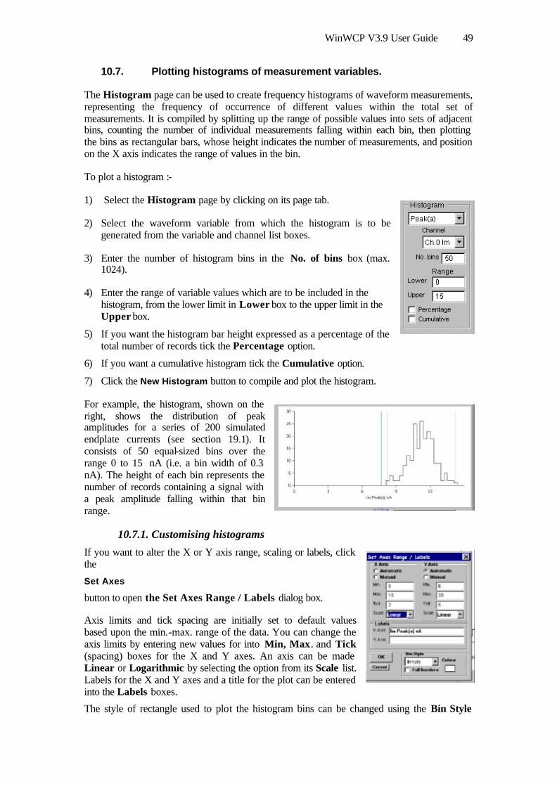
WinWCP V3.9 User Guide 49
10.7. Plotting histograms of measurement variables.
The Histogram page can be used to create frequency histograms of waveform measurements, representing the frequency of occurrence of different values within the total set of measurements. It is compiled by splitting up the range of possible values into sets of adjacent bins, counting the number of individual measurements falling within each bin, then plotting the bins as rectangular bars, whose height indicates the number of measurements, and position on the X axis indicates the range of values in the bin.
To plot a histogram :-
1) Select the Histogram page by clicking on its page tab.
2) Select the waveform variable from which the histogram is to be generated from the variable and channel list boxes.
3) Enter the number of histogram bins in the No. of bins box (max. 1024).
4) Enter the range of variable values which are to be included in the histogram, from the lower limit in Lower box to the upper limit in the Upper box.
5) If you want the histogram bar height expressed as a percentage of the total number of records tick the Percentage option.
6) If you want a cumulative histogram tick the Cumulative option.
7) Click the New Histogram button to compile and plot the histogram.
For example, the histogram, shown on the right, shows the distribution of peak amplitudes for a series of 200 simulated endplate currents (see section 19.1). It consists of 50 equal-sized bins over the range 0 to 15 nA (i.e. a bin width of 0.3 nA). The height of each bin represents the number of records containing a signal with a peak amplitude falling within that bin range.
10.7.1. Customising histograms
If you want to alter the X or Y axis range, scaling or labels, click the
Set Axes
button to open the Set Axes Range / Labels dialog box.
Axis limits and tick spacing are initially set to default values based upon the min.-max. range of the data. You can change the axis limits by entering new values for into Min, Max. and Tick (spacing) boxes for the X and Y axes. An axis can be made Linear or Logarithmic by selecting the option from its Scale list. Labels for the X and Y axes and a title for the plot can be entered into the Labels boxes.
The style of rectangle used to plot the histogram bins can be changed using the Bin Style

WinWCP V3.9 User Guide 50
options. Select No Fill to display bins as rectangular outlines, Solid Fill to fill the bins in with a solid colour, and Hatched Fill for bins filled with a diagonal lines. You can define the colour used for the solid fill, by clicking the Colour box, and selecting a colour from the palette. The Full Borders check box determines whether the outline is drawn completely around each bar, or just where bars do not overlap.
10.7.2. Printing the histogram
To print the displayed histogram, select
File Print
To open the Print dialog box. Click the Print button to plot the graph.
10.7.3. Copying the histogram data points to the Windows clipboard The numerical values of the X,Y data points which generate the histogram can be copied to the clipboard by selecting
Edit Copy Data
The data is placed on the clipboard as a table of data values, in tab text format, defining the histogram. There are 4 values per row, and one row for every bin in the histogram. Each row has the format
<Bin Lower Limit> <tab> <Bin Mid-point> <Bin Upper Limit> <tab> <Bin Count> <cr> <lf>
10.7.4. Copying an image of the histogram to the Windows clipboard
An image of the histogram plot can be copied to the clipboard by selecting
Edit Copy Image
to open the copy image dialog box.
The dimensions (pixels) of the bit map, which will hold the image, can be set using the Width and Height image size boxes. The size and style of the typeface can be set using the Typeface and Size boxes.
When the image parameters have been set, click the OK button to copy the image to the clipboard.

WinWCP V3.9 User Guide 51
10.7.5. Fitting gaussian curves to the histogram Gaussian probability density functions, representing the distribution of discrete populations of events, can be fitted to a histogram using non-linear least squares curve fitting. The number of events expected to be found in each histogram bin for a distribution represented by a mixture of m gaussians is given by
( ) ( )∑=
−−⋅⋅=
m
i i
i
i
i xawNxy
122 2
exp2 σ
µ
πσ
where N is the total number of events (records), w is the histogram bin width and each gaussian, i, is defined by three parameters, its mean, µi, standard deviation, σi and the fraction of the total number of events, ai, contained within it.
To fit a gaussian curve to the displayed histogram :-
1) Select the number of gaussian functions (1, 2 or 3) to be fitted from the equations list.
2) Define the region within the histogram to which the curve is to be fitted using the pair of vertical analysis region cursors. The selected region is indicated by the horizontal bar at the bottom of the display.
3) Click the Fit Curves button to start the curve fitting process. The initial parameter guesses are displayed in the Set Fitting Parameters dialog box. If you want to keep a parameter fixed (i.e. not changed by curve fitting process) tick its Fixed box. You can also change the initial parameter guesses, if they appear to be unrealistic. Click the OK button to fit the curve.
The best fitting curve is superimposed on the X/Y graph (in red) and the best fit equation parameters are displayed in the Curve Fitting table, along with the parameter standard error, the residual standard deviation (between the fitted and data points), statistical degrees of freedom in the fit, and the number of iterations it took to find the best fit.

WinWCP V3.9 User Guide 52
10.8. Summaries of results.
The Summary page displays a summary report containing the mean values and standard errors for the records, which have been analysed.
To display the summary of results,
1) Select the Summary page by clicking on its page tab.
2) Select the channel to be summarised from the Channel list.
3) Select the variables to be included in the summary by ticking or un-ticking the appropriate variable tick box.
A table like that shown here will be displayed.
10.9. Tabulating lists of results
The Tables page is used to display lists of measurements in tabular form.
To display lists of data
1) Select the Tables page by clicking on its tab.
2) Define one or more data columns by double-clicking on the top row of the selected column to get the Set Variable dialog box.
and select the variable to be listed and the channel from which it is obtained.
To print out a copy of a summary report or table of results on the printer, select
File Print
To copy the report or table to the Windows clipboard, select
Edit Copy Data

WinWCP V3.9 User Guide 53
11. Curve Fitting
11.1. Introduction
The curve fitting module allows a number mathematical functions to be fitted to digitised signal waveforms. A mathematical model consists of a general equation representing the time course of the signal (or part of the signal) under study. For instance, the decay of many signals (e.g. endplate currents) can be represented by an exponential function
f t At
( ) exp( )=−τ ,
where A is the amplitude of the signal and τ is the decay time constant. Expressed as above, the equation is quite general applying to any signal, depending on the values of the parameters A and τ.
In order to determine whether the equation actually does provide a good model of the signal decay it is necessary to find the parameter values which provides the best match (or fit) of the theoretical curve to an actual signal. This can be done using the process know as iterative curve fitting. Starting with initial guesses for the parameters, the theoretical curve is compared with the experimental data points, the parameters are adjusted to try to improve the fit, and the process is repeated until no more improvement can be obtained.
The quality or goodness of the fit between theoretical curve and the data is determined from the sum of the squared differences (S) between a set of n data points, y(i) (i=1..n), and the theoretical curve, f(i), computed at the same sample time points, i.e.
( ) ( )( )2
1∑
=
−=n
i
ifiyS
The best fit is found by repeatedly computing S, at each iteration adjusting the equation parameters using a strategy to minimise S. The best fit parameters are the ones which yield a minimum value of S. WinWCP uses a modified Levenberg-Marquardt least squares minimisation algorithm (the SSQMIN routine, developed by Kenneth Brown at the University of Cincinnatti). (A more detailed discussion of curve fitting algorithms can be found in Chapter 6 of Dempster, 1993.)
11.2. Fitting curves to digitised signals
To open the curve fitted module, select
Analysis Curve Fit
The module is split 5 functional sections (pages) – Curve Fitting, X/Y Plot, Histogram, Summary, Table - accessed by clicking on the page tab.
The Fit Curve page is used to select the region of the signal and equation to be fitted and initiate the curve fitting process.
The X/Y plot page is used to create X-Y graphs of the measurements.

WinWCP V3.9 User Guide 54
The Histogram page is used to create frequency histograms of measurement.
The Summary page presents a summary (mean, standard deviation, etc.) of the measurements for the series of records analysed.
The Tables page is used to create tables of results.
11.3. Running a curve fitting sequence
The first stage in the curve fitting process is to select an equation and run a curve fitting sequence on selected parts of a series of records.
1) Select the Curve Fit page by clicking on its page tab.
2) Select the equation to be fitted to the record(s).
3) Select the channel containing the signal trace to which the curve is to be fitted, from the Ch. list.
4) Define the range of records to be analysed, by selecting All Records to analyse all records, or This Record to analyses only the currently displayed record, or Range and enter a range of records.
5) Select the type of records to be measured by selecting an option from the Type list. Select ALL to measure records of any type (except rejected records).
6) Select Manual or Automatic Data Cursors mode. In manual mode, the region within the signal to which the curve is to be fitted is set manually using a set of 3 cursors on the display. In automatic mode, the curve fitting region is set automatically.
7) If you have selected Automatic Data Cursor mode, select On Rise, On Decay or Rise+Decay, to determine whether the cursors are to be placed on the rising phase, decaying phase, or complete time course of the signal waveform. Then enter the levels on the waveform where the cursors are to be placed in the Limits box. (Default setting is 10-90%, placing the cursors at 10% and 90% of peak amplitude on the selected phase)
8) If you have selected Manual Data Cursors mode, define the curve fitting region by using three vertical cursors – two (blue, marked |) define the region to which the equation is to be fitted, the third (green, marked t0) defines where the zero time points for the equation is. (Note that the choice of fitting region depends upon the kind of curve being fitted. Sometimes, only part of the signal is chosen, such as when an exponential curve is to be fitted to the decay phase of the signal. In the example shown here, the fitting region cursors have been placed on the decay phase of an endplate current. Zero time (t0) has been defined at the onset of the signal.)

WinWCP V3.9 User Guide 55
9) If you wish to change the initial values for the equation parameters, or fix some parameters so they do not change during the fit, click the Set Parameters button to open the Set Fitting Parameters dialog box. If you want to keep a parameter fixed at a set value, enter the value into the appropriate parameter box and click the Fixed check box.
10) When all curve fitting settings have been made, click the Do Fit button to initiate the curve fitting sequence.
The iterative curve fitting process now begins. The SSQMIN routine iterates through a variety of trial parameter sets, until no more improvement can be obtained. The number of iterations are displayed as fitting progresses. The best fit is usually found within 10-20 iterations. Fitting is aborted if the process has not converged to a suitable answer within 100 iterations, and can also be aborted by clicking the Abort button.
11.4. Curve fit results
For each record fitted, the best fit curve is indicated by a red curve superimposed on the blue signal trace.
A residuals trace is shown below indicating the difference between the fitted curve and the data.
The parameters of the best fitting equation are shown in the Results table, along with the parameter standard error, the residual standard deviation (between the fitted and data points), statistical degrees of freedom in the fit, and the number of iterations it took to find the best fit.
11.5. Plotting and tabulating results
X/Y graphs, histograms, summaries and tables of the best fit equation parameters can be produced using the X/Y Plot, Histogram, Summary and Table pages of the curve fitting module. These options are identical in function to the corresponding pages in the waveform measurement module and are therefore not repeated here. (See sections 9.5- 10.7 for details of their use.)

WinWCP V3.9 User Guide 56
11.6. Equations
Straight line CxMxy +⋅=)(
Exponential (general) C
Taux
Axy +
−
⋅= exp)(
Decaying Exp.
−
⋅=Tau
xAxy exp)(
2 Exponential (general) C
Taux
ATau
xAxy +
−
⋅+
−
⋅=2
exp21
exp1)(
2 Decaying Exps.
−
⋅+
−
⋅=2
exp21
exp1)(Tau
xA
Taux
Axy
3 Exponential C
Taux
ATau
xA
Taux
Axy +
−
⋅+
−
⋅+
−
⋅=3
exp32
exp21
exp1)(
3 Decaying Exps.
−
⋅+
−
⋅+
−
⋅=3
exp32
exp21
exp1)(Tau
xA
Taux
ATau
xAxy
Endplate current ( )
−−⋅
−
+⋅⋅=TauD
xxTauR
xxerfAxy
0exp
015.0)(
The endplate current rising phase is modelled by error function and the decay with an exponential function.
H-H (K)
P
TauMx
Axy
−−⋅= exp1)(
The time course of activation of a voltage-activated current with Hodgkin-Huxley kinetics
H-H (Na) ( )
−−−
−−⋅=
TauHx
HHTauM
xAxy
P
exp1infinfexp1)(
The time course of a current with voltage dependent activation and inactivation following Hodgkin-Huxley kinetics (e.g. sodium current). (Note. It is assumed that, initially, the activation parameter, m=0 and inactivation parameter, h=1.)
WinWCP V3.9 User Guide 57
11.6.1. Assessing the quality of a curve fit Iterative curve fitting is a numerical approximation technique, which is not without its limitations. In some circumstances, it can fail to converge to a meaningful answer, in others the best fit parameters may be poorly defined. It is important to make an assessment of how well the function fits the curve before placing too much reliance on the parameters.
11.6.2. Does the chosen function provide a good fit to the data? One assessment of the goodness of fit is to compare the variance of the residual differences between the best fit function and the data with the background variance of the signal. If the function provides a poor fit to the data, the residual variance will be significantly greater than the variance of the random background noise on the signal. The distribution of the variance as displayed in the residuals plot is also important. Deviations should be randomly distributed over the fitted region of the record. If the fitted line is consistently higher than the data points in some parts and lower in others this indicates that the signal is not well represented by the chosen equation.
11.6.3. Are the parameters well-defined?
The aim of most curve fitting exercises is to obtain a well-defined set of function parameters (e.g. exponential time constants) which characterise the part of the signal being fitted. The standard errors of the best fit parameters provide an indication of this. A large standard error indicates that a parameter is poorly defined by the data and can be varied significantly with little effect on the goodness of fit. Such a situation typically arises when there is insufficient information contained in the signal waveform to adequately define the function. For instance, in the case of exponential functions, the waveform data must be of sufficient duration to contain at least one time constant of the exponential function before an accurate estimate can be obtained. Similarly, it proves difficult to accurately estimate the time constants of multiple exponential functions when they differ by less than a factor of 5.
It is worth noting that the parameter "standard errors" discussed above are computed from the Hessian matrix by the curve fitting program, and are not true estimates of experimental standard error since they take no account of inter cell or other variability. In addition, they only provide a lower bound to the estimate of the standard error in parameter value. It can be shown (by simulation) that, if the random noise on the experimental signals is correlated, then the variability of fitted parameters may be substantially greater than suggested by the computed parameter standard error. The error in parameter estimation can be a complex function of the parameter values and the signal-noise ratio of the data. It is therefore wise to test the curve fitting procedure using simulated waveforms with known parameters set spanning the range of values likely to be observed in the experimental data.
11.6.4. Are all the parameters meaningful? It is also necessary to discriminate between functions, which fit the data equally well. For instance, the question often arises as to whether one, two, or more, exponential functions are needed to fit a signal waveform. It is usually obvious from the residual plot when a single exponential does NOT provide a good fit. However, when a single exponential does fit, two or more exponentials will also provide a good fit. In such circumstance, it is usual to choose the function with the least number of parameters, on the principle of parsimony. An excess of function parameters also results in the some of the parameters being ill-defined with standard errors values often larger than the parameter values themselves.
A more detailed discussion of the above issues can be found in Dempster (1992) and (2001).

WinWCP V3.9 User Guide 58
12. Signal Averaging
12.1. Principles of signal averaging
Many electrophysiological signals have poor signal-noise ratios, making it difficult to obtain accurate measurements from individual records. However, if a signal can be made to occur repeatedly, digital signal averaging techniques can recover the signal waveform from the background noise.
The signal average of a series of records is generated by computing the average of each corresponding sample within the records. For a set of N records, consisting of samples, yi, (i=1,n) the average record consists of n samples, and is given by.
i ir
N
Avg yN
==
∑1
1
12.1
The location of signals within the record sometimes varies from record to record, due to imperfections in the detection of spontaneous signals or fluctuations in stimulus latency. In such circumstances, averaging corresponding sample points within the record would result in a distorted signal average. This problem can be avoided by aligning the signals by the mid-points of their rising phases before averaging.
12.2. Creating signal averages
To compute signal averages from records stored in a digitised data file, select
Analysis Signal Averager
to open the signal averager module.
To create the averages:
1) Specify the range of records to be averaged by entering the first and last records, separated by a “-“, in the range box.
2) Enter the number of records to be included in each average in the in blocks of box. (Note. The default settings produce a single average record from all the records in the data file.)
3) You can restrict averaging to a specific type of record by selecting a type from the type list. Select ALL to use records of any type (except rejected records).
4) Set the alignment mode. Select No alignment if the position of the signals do not vary within the records and alignment is not necessary. If alignment is necessary, select on positive rise for positive-going signals and on negative rise for negative signals.
5) Set the alignment search region cursors. If records contain stimulus artefacts, it may be necessary to restrict the region of the record which is searched for the signal mid-point, in order to avoid the averages being aligned using the artefacts rather than the true signals. The alignment search region is set by moving the two vertical cursors on the display to define the beginning and end of the region containing the signal.

WinWCP V3.9 User Guide 59
6) To create the averages, click
Do Averages
The averaging process now proceeds. An additional digitised data file is created to contain the average record(s), with the same name as the original data file, but with a ".AVG" file extension rather than ".WCP".
12.3. Viewing averaged data records
On completion of averaging, the record display module is opened to show the average records. You can switch the display back and forth between the averages file and the raw data file by selecting
View Averaged Records
To view the averages, and
View Raw Records
To view the original digitised signal records.

WinWCP V3.9 User Guide 60
13. Digital subtraction of leak currents
Ionic currents recorded using the voltage clamp technique are usually composed of a variety of components, mediated by different ionic channels (e.g. Na, K, Ca, Cl etc.). In order to study a particular current in detail, it is usually necessary to eliminate all the other currents from the signal. This is often done using pharmacological agents, such as TTX to block Na currents, TEA to block K currents, etc. However, even when such blocking agents are used, there often still remains some residual current in addition to the one under study. This current, is known as the leak current. It usually displays linear time-independent properties. In some circumstances, the leak current is very small and can be ignored. However, in others it can be as large as the currents under study, complicating the analysis of the signal waveforms unless it is removed.
Although the leak current cannot be removed pharmacological, its linear properties permit a digital subtraction approach to be used. The current signal can be considered to consist of 3 components
I t I t I t It c i lk( ) ( ) ( )= + + 12.1
where Ii(t) is the time-dependent, voltage-activated, ionic current under study, Ilk is the leak current, and Ic(t) is transient capacity current due to the charging and discharging of the membrane capacity. Ic(t) and Ilk are always present in the signal, and scale linearly with the size of the voltage step. However, Ii(t) only occurs for voltage steps to potentials which activate the voltage sensitive ion channels. The Na current, for instance, is only evoked by depolarising voltage steps to potentials more positive than -60mV. It is possible to obtain a record, containing only leak and capacity currents, by using a hyperpolarising voltage step (or a small depolarising step)
I t I t Is c lk( ) ( )= + 12.2
Scaling this record to account for the differences in the size and/or polarity of the voltage step, and subtracting it from the test record, effectively removes the leak and capacity currents.
I t I t I tVVi t s
t
s
( ) ( ) ( )= − 12.3
Since the scaling up of small subtraction records also scales up the background noise, it is usual to average several subtraction records before, scaling and subtracting. It is also possible to average the test records. WinWCP uses the following general algorithm
I tM
I tV
NVI ti t
t
si
M
sj
N
( ) ( ) ( )= += =
∑ ∑1
1 1
12.4
where M is the number of test records averaged and N the number of subtraction records.
13.1. Recording protocols for leak subtraction.
One of the most commonly used leak subtraction protocols is the P/N protocol, developed by Bezanilla & Armstrong (1977). For each depolarising test pulse, there are N additional subtraction pulses, evoked by hyperpolarisng pulses 1/Nth the amplitude of the test pulse.
WinWCP's stimulus generator can be configured to produce the necessary sequence of test and leak subtraction recording sweeps, by selecting the P/N Mode leak subtraction option (see section 8). This causes the stimulus generator to produce additional scaled down and inverted stimulus pulse waveforms for evoking the linear leak currents without the voltage-activated currents. The leak current recordings are averaged and stored in a record marked as a LEAK type. The test record is marked as TEST type record. The TEST record, with its

WinWCP V3.9 User Guide 61
associated LEAK record, are collected together in a group (i.e. they have the same group number).
13.2. Subtracting leak currents
To subtract the leak currents from a data file
1) Open the leak current subtraction module by selecting Analysis Leak Current Subtraction
2) Select the channel containing the cell membrane potential from the Voltage channel list.
3) Select the channel containing the cell membrane current from the Current channel list.
4) Select the source of the Leak records . If records are grouped into LEAK/TEST record pairs, select From Group (This option should be used for P/N protocols). If the LEAK records are not grouped with the TEST records, select From whole file . (Whole file mode is used when one or more records at the beginning or end of a data file are to be used as LEAK records. Note that these records will have to be manually classified as LEAK).
5) Set the current Scaling mode. Select From Voltage to use the ratio between the TEST and LEAK voltage pulses as the current scaling factor (default). Select Fixed if you wish to use the fixed scaling factor, entered in the box below. (Fixed mode is required when the record does not contain a voltage channel.)
6) If you have selected the From Voltage scaling mode, use the VTest and VHold display cursors to define the measurement points on the voltage trace used to compute the voltage scaling. VHold is placed over the holding voltage level and VTest is placed over the mid-point of the test voltage. (An average of 20 samples around each measurement point is used to compute the voltage levels.).
7) Select
Do subtraction
To initiate the leak subtraction process.
For each group of records, the LEAK and TEST records are averaged, scaled and subtracted, using equation 12.4. Each group is condensed down to one leak-subtracted record that is stored in a .SUB file with the same name as the data file. These records can then be displayed and analysed using the View Records, Waveform analysis, and Curve fitting modules, by selecting
View Leak subtracted

WinWCP V3.9 User Guide 62
14. Non-stationary noise analysis
The non-stationary noise module analyses the random fluctuations in the decay of ion channel currents, providing an estimate of single-channel current and total number of channels in the fluctuating population. For a cell containing a population of n ion channels, each capable of passing a current i, the mean whole cell current, Im(t) is,
( ) ( )tpnitI m ⋅⋅= 13.1
where p(t) is the probability of a channel being open at time t. The variance, σ2(t), of the current fluctuations, at time t, about this mean is,
( ) ( ) ( )( )tptpnit −⋅⋅⋅= 122σ 13.2
These two equations can be combined to provide a relationship between σ2(t) and Im(t),
( ) ( ) ( )ntI
tIit mm
22 −⋅=σ 13.3
The single-channel current, i, and number of channels, n, can thus be calculated by fitting the above parabolic function to a plot of σ2(t) vs Im(t) during a current transient where p(t) is changing. Im(t) can be computed as the average current of a series of transient current records, repeated M times all evoked by the same stimulus,
( )( )
M
tytI
M
jj
m
∑== 1 13.4
The variance, σ2(t), at each sample point, t, can similarly be computed from
( )( ) ( )( )
11
2
2
−
−=
∑=
M
tItyt
M
jmj
σ 13.5
The method was developed by Sigworth (1981) for voltage-activated Na currents. It has also been used to study the fluctuations during the rapidly desensitising currents induced by high concentrations of acetylcholine (Dilger & Brett, 1990). With modification it can also been applied to synaptic currents. The basic non-stationary variance approach assumes that the only source of variance arises from the fluctuations of the ion channels that carry the current. However, synaptic current amplitude can fluctuate due to both ion channels and quantal size/content variation. Traynelis et al (1993) found a way round this problem by scaling the amplitude of the average current to the peak amplitude of each signal before the subtraction in Eqn. 13.5, thus compensating for the quantal variation. This approach does have limitations and it is worth reading De Koninck & Mody (1994) if considering using the scaling approach.
To compute the single-channel current and number of channels from a series of ionic current transient :-
1) Collect a series of 100-200 records containing the transient signal under study.
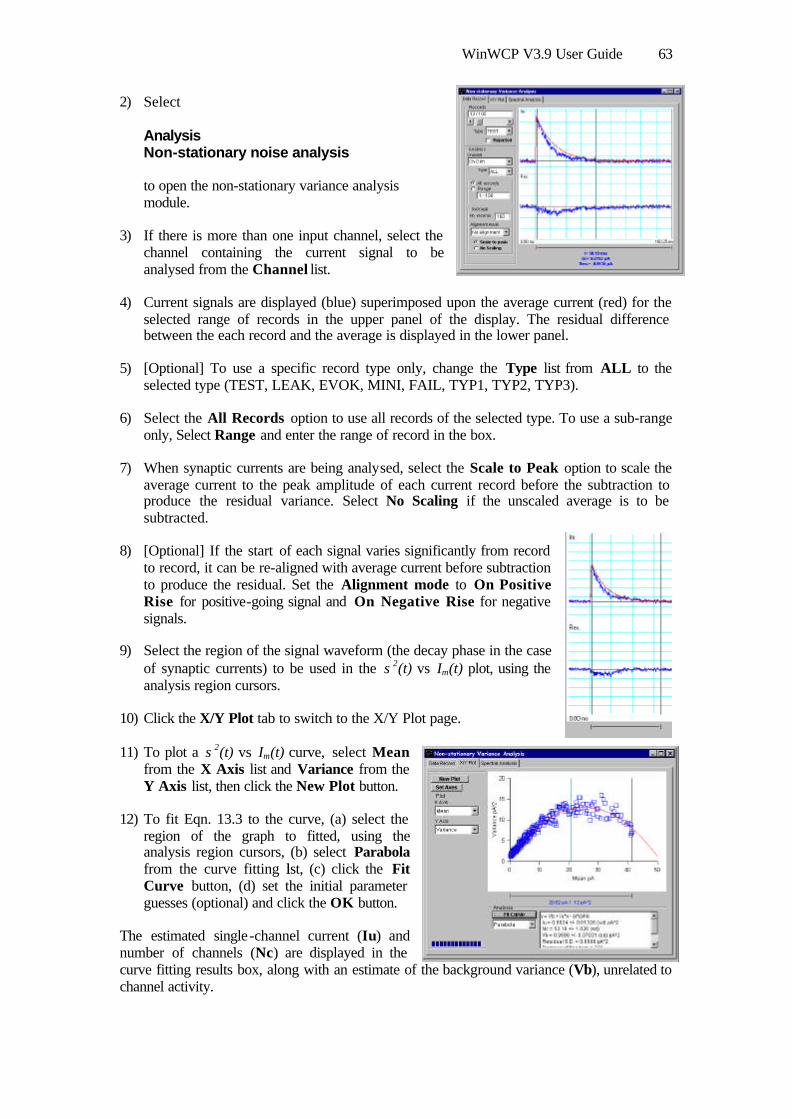
WinWCP V3.9 User Guide 63
2) Select Analysis Non-stationary noise analysis to open the non-stationary variance analysis module.
3) If there is more than one input channel, select the channel containing the current signal to be analysed from the Channel list.
4) Current signals are displayed (blue) superimposed upon the average current (red) for the selected range of records in the upper panel of the display. The residual difference between the each record and the average is displayed in the lower panel.
5) [Optional] To use a specific record type only, change the Type list from ALL to the selected type (TEST, LEAK, EVOK, MINI, FAIL, TYP1, TYP2, TYP3).
6) Select the All Records option to use all records of the selected type. To use a sub-range only, Select Range and enter the range of record in the box.
7) When synaptic currents are being analysed, select the Scale to Peak option to scale the average current to the peak amplitude of each current record before the subtraction to produce the residual variance. Select No Scaling if the unscaled average is to be subtracted.
8) [Optional] If the start of each signal varies significantly from record to record, it can be re-aligned with average current before subtraction to produce the residual. Set the Alignment mode to On Positive Rise for positive-going signal and On Negative Rise for negative signals.
9) Select the region of the signal waveform (the decay phase in the case of synaptic currents) to be used in the σ2(t) vs Im(t) plot, using the analysis region cursors.
10) Click the X/Y Plot tab to switch to the X/Y Plot page.
11) To plot a σ2(t) vs Im(t) curve, select Mean from the X Axis list and Variance from the Y Axis list, then click the New Plot button.
12) To fit Eqn. 13.3 to the curve, (a) select the region of the graph to fitted, using the analysis region cursors, (b) select Parabola from the curve fitting list, (c) click the Fit Curve button, (d) set the initial parameter guesses (optional) and click the OK button.
The estimated single-channel current (Iu) and number of channels (Nc) are displayed in the curve fitting results box, along with an estimate of the background variance (Vb), unrelated to channel activity.

WinWCP V3.9 User Guide 64
15. Quantal analysis of transmitter release
The quantal analysis module can be used to estimate the quantal content of neuromuscular nerve-evoked endplate currents or potentials, and other forms of synaptic signal, using the either the direct method, variance method, and method of failures. In circumstances where both evoked and spontaneous miniature events are available, transmitter release parameters, n, (number of available quanta) and p, probability of release, is calculated using binomial analysis.
15.1. Quantal content (direct method)
If the data file contains both evoked and miniature signals, the direct method of calculating quantal content can be used.
QCAvg PeakAvg Peakdirect
evoked
i
=( )( )min
14.1
This is the most accurate method for calculating quantal content.
15.2. Quantal content (variance method)
It is not always possible to record the miniature synaptic signals, which represent single quanta. In such circumstances, it may still be possible to calculate quantal content from the variability of the evoked signal
( )( ) ( )BackgroundVarPeakVar
PeakAvgQC
evoked
evoked
−=
2
14.2
This method is dependent upon the assumption that the number of quanta released follows a Poisson distribution. This will only be the case when the probability of release is very low (i.e. p < 0.1). Since large errors can result if this condition is not satisfied, results using the variance method should be treated with caution.
15.3. Quantal Content (failures method)
If the quantal release probability is very low, a nerve stimulus may occasionally release no quanta at all, resulting in intermittent failures to evoked post-synaptic signals. Again using the assumption of a Poisson distribution controlling release, the quantal content can be calculated from
QCNNf e
stimuli
failures
= log ( ) 14.3
15.4. Binomial analysis
The transmitter release process can often be modelled as a pool of n quanta available for release, with each quantum having a probability, p, of being released when the nerve is stimulated. If both evoked and spontaneous signals are available, it is possible to calculate estimates for n and p, on the assumption that the number of quanta released per stimulus follows a binomial distribution.
{ }{ } { } { }evokedminievoked
evoked
PeakVarPeakAvgPeakAvgPeakAvg
n−⋅
=2
14.4

WinWCP V3.9 User Guide 65
pAvg Peak
n Avg Peakevoked
i
=⋅
( )( )min
14.5
15.5. Correction for non-linear summation of potentials
Unlike currents recorded under voltage-clamp conditions, synaptic potentials do not summate linearly. Therefore the size of the synaptic potential is not directly proportional to the number of quanta released. However, given certain assumptions, it is possible to correct for the effects of non-linear summation using the eqn.
( )rmevoked
evoked
VVPeakfPeak
Peak−⋅⋅−
=1
14.6
where Peakevoked is the measured peak amplitude of the evoked synaptic potential, Vm is the cell resting potential, Vr is the reversal potential for the post-synaptic ion channels, and f is a correction factor for the effects of the cell membrane time constant on synaptic potential amplitude. (A discussion on non-linear summation and its correction can be found in McLachlan & Martin, 1981).
15.6. Quantal content calculation procedure
The following procedure can be used to calculate the quantal content of a series of synaptic currents or potentials, which have been recorded and stored in a digitised data file.
1) Using the record display module, inspect each record in the data file and classify it as being either a nerve-evoked signal, EVOK, a spontaneous miniature event, MINI, or (in experiments where the probability of transmitter release is low) a nerve stimulus which has failed to release any quanta, FAIL. (You should also mark any records containing artefacts as REJECTED.).
2) Use the waveform measurements module to calculate the waveform parameters for ALL of the records, with the intention of measuring the signal peak amplitude (Take care to exclude the nerve stimulus artefact).
3) Select Analysis Quantal Content to invoke the quantal analysis module.
1) Select the type of analysis. Choose Poisson if there are no MINI records available and the transmitter release probability is expected to be low. Otherwise choose Binomial.
2) Enter the range of records to be used in the analysis. Select All records if you want to use all records in the file, or select Range and enter a range of records.
3) If there are several channels in the signal record, select the channel which contains the signals to be analysed, from the Ch. list.
4) Evoked events . Select the EVOK record classification type, used to indicate stimulus-

WinWCP V3.9 User Guide 66
evoked signals, from the Type list.
5) Quantum events. If the file contains miniature events, select the Events in file option and select MINI from the Type list. If there are no miniature events in the file, but you know what the quantal signal amplitude is, select User entered and enter the average peak amplitude of the spontaneous miniature signal into the Amplitude box, and the standard deviation of peak amplitude in the Standard Dev. box
6) Analysis mode . If the signals being analysed are currents, recorded under voltage-clamp conditions, select the Currents option. If the signals are potentials, select the Potentials option, and enter the cell resting potential and the reversal potential of the synaptic conductance into the Resting potential and Reversal potential boxes. This data is used to apply a correction for the non-linear summation effect. The Correction factor should be left at the default value (1) unless the appropriate factor for the synapse under study is known.
7) Click the Do Analysis button, to begin the quantal analysis sequence.
The analysis procedure scans through the data file, calculates the mean and variance of the peak amplitude of the signal records, uses these to obtain estimates for the quantal content, and displays the results in the report window. A copy of the quantal analysis report is also written to the log file.
(Note that you can test the operation of the quantal content analysis module using simulated endplate currents or potentials, generated by the synaptic signal simulation module. See section 19.1.)

WinWCP V3.9 User Guide 67
16. Synaptic current driving function analysis
The synaptic current driving function is a measure of the rate of evoked release of transmitter at a synapse. If the time course of decay the post-synaptic current is known, the driving function can be computed using a deconvolution process. More details of the method can be found in Dempster (1984). WinWCP’s driving function module can be used to compute the driving function from synaptic current records, such as endplate currents.
To carry out a driving function analysis :-
1) Record a series of stimulus-evoked synaptic currents.
2) Use the signal averaging module to create an average synaptic current from the set of raw records.
3) Use the curve fitting module to fit an exponential function to the decay phase of the averaged synaptic current. Fit the function from around 95% - 5% of the decay phase, excluding the 5% around the peak where the transmitter is still being release.
4) To open the driving function module, select Analysis Driving Function
5) If there are several channels in the record, select the channel containing the signal to be transformed from the Ch. list.
6) Set the range of records to be transformed. Select All Records for all the records in the file, This Record for the currently displayed record only, or select Range and enter a range of records into the box.
7) Enter the cell holding potential (in mV) that the currents were recorded at, in the Holding Potential box, and the reversal potential of the post-synaptic current, in the Reversal Potential box. (The driving function is expressed in units of conductance/unit time. The holding and reversal potentials are required to convert from current to conductance).
8) The time constant computed by the curve fitting module in step (3) is used to deconvolve the current signal. If you wish to use the same time constant for all records (rather than using the individual value computed from each record), select the Keep parameters fixed option.
9) The basic deconvolution process computes a driving function, which represents the rate of change of post synaptic conductance induced by the release of transmitter. It is also possible to reconvolve this driving function with a different post-synaptic current decay function to generate the waveform of the synaptic current that would have existed under these new conditions. If you wish to create a simulated current, select the Reconvolute waveform option and enter the new time constant in the Reconvolution column.
10) Click the Do Transforms button to begin the deconvolution process.
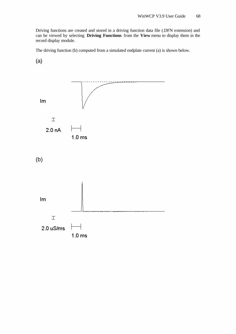
WinWCP V3.9 User Guide 68
Driving functions are created and stored in a driving function data file (.DFN extension) and can be viewed by selecting Driving Functions from the View menu to display them in the record display module.
The driving function (b) computed from a simulated endplate current (a) is shown below.
(a)
(b)
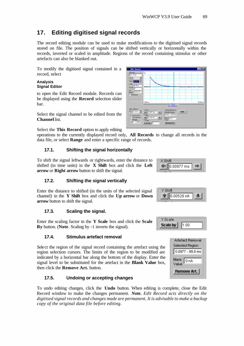
WinWCP V3.9 User Guide 69
17. Editing digitised signal records
The record editing module can be used to make modifications to the digitised signal records stored on file. The position of signals can be shifted vertically or horizontally within the records, inverted or scaled in amplitude. Regions of the record containing stimulus or other artefacts can also be blanked out.
To modify the digitised signal contained in a record, select
Analysis Signal Editor
to open the Edit Record module. Records can be displayed using the Record selection slider bar.
Select the signal channel to be edited from the Channel list.
Select the This Record option to apply editing operations to the currently displayed record only, All Records to change all records in the data file, or select Range and enter a specific range of records.
17.1. Shifting the signal horizontally
To shift the signal leftwards or rightwards, enter the distance to shifted (in time units) in the X Shift box and click the Left arrow or Right arrow button to shift the signal.
17.2. Shifting the signal vertically
Enter the distance to shifted (in the units of the selected signal channel) in the Y Shift box and click the Up arrow or Down arrow button to shift the signal.
17.3. Scaling the signal.
Enter the scaling factor in the Y Scale box and click the Scale By button. (Note . Scaling by -1 inverts the signal).
17.4. Stimulus artefact removal
Select the region of the signal record containing the artefact using the region selection cursors. The limits of the region to be modified are indicated by a horizontal bar along the bottom of the display. Enter the signal level to be substituted for the artefact in the Blank Value box, then click the Remove Art. button.
17.5. Undoing or accepting changes
To undo editing changes, click the Undo button. When editing is complete, close the Edit Record window to make the changes permanent. Note. Edit Record acts directly on the digitised signal records and changes made are permanent. It is advisable to make a backup copy of the original data file before editing.

WinWCP V3.9 User Guide 70
18. Data files
WinWCP uses its own custom data file format for storing digitised signal records. These files are identified by the file extension “.WCP” Data can also be imported from and exported to files in the Axon Binary Format (used by Axon Instruments’ pClamp program) and the Cambridge Electronic Design CFS (CED Filing System) formats. Data can also be imported and exported in the form of ASCII text.
18.1. Opening a existing WCP data file
To load a previously created WCP data file, select
File Open
to display the Open File dialog box. Select the disk drive and folder from the Look In list. A list of available WCP files will be displayed.
Select one of the file names, then click the OK button to open the data file for display and analysis.
18.2. Appending a WCP data file
To append a WCP data on to the end of the currently open file, select
File Append
To display the Append File dialog box. Select a file (as above) for appending. (Note. You can only append files, which have compatible record sizes with the same number of channels and samples per channel.)
18.3. Importing from foreign data file formats
To import records from a non-WCP data file, select
File Import
To display the Import File dialog box.
Select the disk drive and folder from the Look In list. Then select the type of data file to be imported from the Files of Type list. A list of available files in that type are displayed.

WinWCP V3.9 User Guide 71
Select one of the file names, then click the OK button to import the data into a .WCP format file. (Note that the original file is not changed. A new .WCP format file is created with the same name as the imported file but with the extension.WCP).
18.3.1. Axon Instruments.
Data files produced by Axon Instruments’ pClamp V5 and V6 programs. The files should contain episodic data records, such as created by the CLAMPEX program. Axon data files have a .DAT file extension.
18.3.2. Cambridge Electronic Design
Data files produced by CED’s Voltage & Patch Clamp program, in the CFS (CED Filing System) format. CFS files have a .DAT file extension.
18.3.3. ASCII text files.
Files with the sample values stored as ASCII text in tab text format. The Data File Import dialog box allows you to view the format of the ASCII data to be imported and to specify how it should be imported.
The data must consist of rows of samples (each row terminated by a carriage return + line feed pair of characters ( <cr> <lf> ). Channel sample values within each row are separated by <tab> characters.
The number of signal channels in the record to be created is determined from the number of columns in the table, with one of the columns (usually the first) assumed to contain the time.
The first data row(s) in ASCII table often contain labels or identification information, which should not be treated as samples. To skip one or more of these lines, enter the number to skipped in the No. of initial rows to ignore .
By default, column 1 is assumed to contain the time that each block of samples was acquired. If the time data is contained in a different column, enter the correct column number in the Time data column box. (If there is no time data at all, set Time data column = 0).
The sampling interval is derived from the times of adjacent rows. If there is no time data (or if the displayed interval is wrong) enter the correct value in the Sampling interval box.
Select the units that the time data is expressed in from the Time units list.
Click the OK button, to import the data when the import settings are complete.
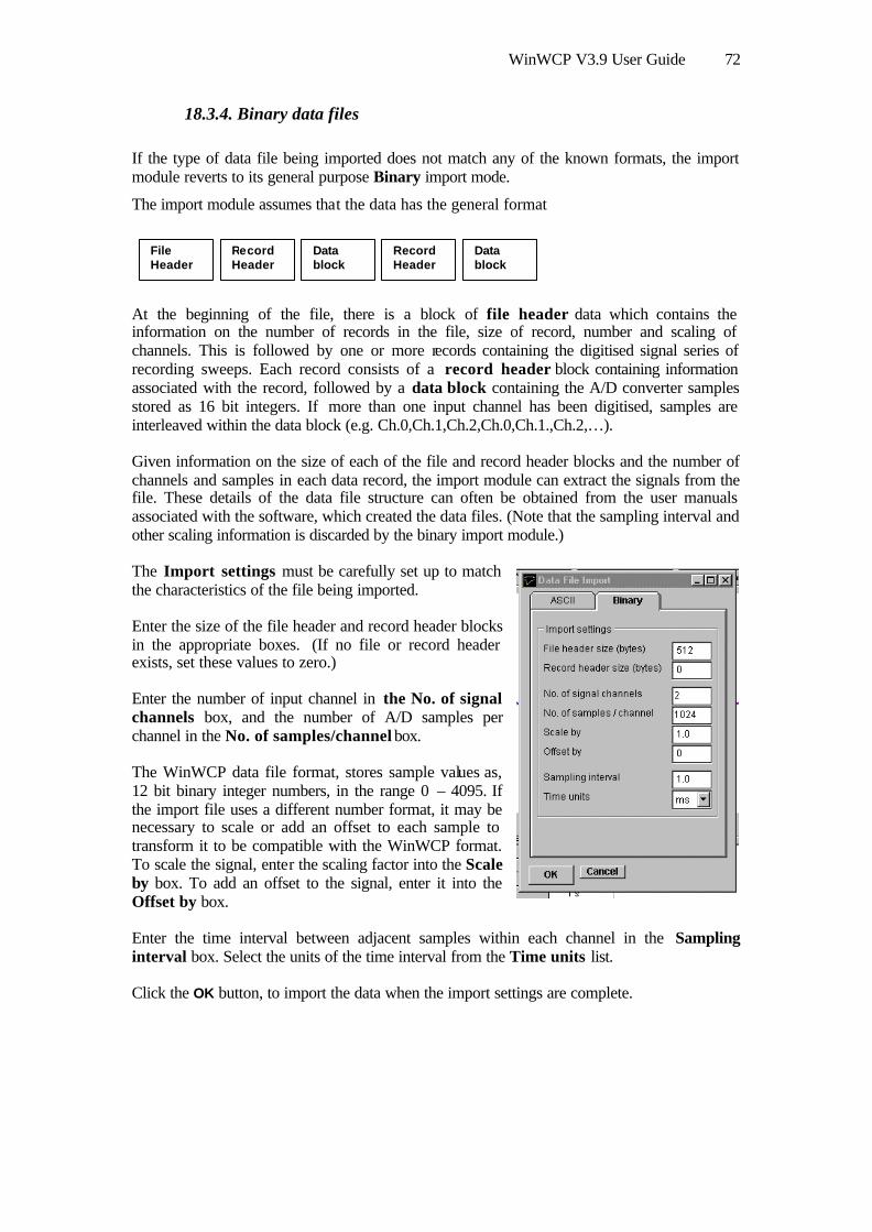
WinWCP V3.9 User Guide 72
18.3.4. Binary data files
If the type of data file being imported does not match any of the known formats, the import module reverts to its general purpose Binary import mode.
The import module assumes that the data has the general format
At the beginning of the file, there is a block of file header data which contains the information on the number of records in the file, size of record, number and scaling of channels. This is followed by one or more records containing the digitised signal series of recording sweeps. Each record consists of a record header block containing information associated with the record, followed by a data block containing the A/D converter samples stored as 16 bit integers. If more than one input channel has been digitised, samples are interleaved within the data block (e.g. Ch.0,Ch.1,Ch.2,Ch.0,Ch.1.,Ch.2,…).
Given information on the size of each of the file and record header blocks and the number of channels and samples in each data record, the import module can extract the signals from the file. These details of the data file structure can often be obtained from the user manuals associated with the software, which created the data files. (Note that the sampling interval and other scaling information is discarded by the binary import module.)
The Import settings must be carefully set up to match the characteristics of the file being imported.
Enter the size of the file header and record header blocks in the appropriate boxes. (If no file or record header exists, set these values to zero.)
Enter the number of input channel in the No. of signal channels box, and the number of A/D samples per channel in the No. of samples/channel box.
The WinWCP data file format, stores sample values as, 12 bit binary integer numbers, in the range 0 – 4095. If the import file uses a different number format, it may be necessary to scale or add an offset to each sample to transform it to be compatible with the WinWCP format. To scale the signal, enter the scaling factor into the Scale by box. To add an offset to the signal, enter it into the Offset by box.
Enter the time interval between adjacent samples within each channel in the Sampling interval box. Select the units of the time interval from the Time units list.
Click the OK button, to import the data when the import settings are complete.
File Header
Record Header
Data block
Record Header
Data block

WinWCP V3.9 User Guide 73
18.4. Exporting to foreign data files
WCP data files can also be exported a number of data file formats. To export the currently open data file, select
File Export
To open the Export file dialog box.
Select the disk drive and folder where the exported file is to be stored from the Look In list. The export file name is initially set to the same name as the WCP file, but with a .DAT file extension.
Files can currently be exported in Axon Instruments data file formats.
18.5. Experiment Log file
WinWCP maintains a log file of the operations initiated by the user during the course of recording or analysing an experiment. The names of data files created or loaded, comments entered, stimulus programs used, and other events are stored along with the time that the event occurred. The log file can be used like an experimenter's notebook to keep a written record of the experiment.
A new log file is opened on a daily basis with a name in the form dd-mm-yy.log and stored in the WinWCP program directory.
To display the experimental log, select
File Inspect Log File

WinWCP V3.9 User Guide 74
19. Simulations
The simulation modules can be used to generate data files containing simulated waveforms, with known characteristics, which can be used to test the operation of the measurement and analysis modules. Three kinds of waveform can be simulated, nerve-evoked EPSCs, voltage activated ionic currents and spontaneous miniature EPSCs.
19.1. Nerve-evoked EPSCs
The nerve-evoked EPSC module generates a series of nerve-evoked excitatory post-synaptic currents (EPSCs) or potentials (EPSPs). When the nerve is stimulated a random number of transmitter quanta are released from a pool of size, n, with each quantum having a probability, p, of release. The number of quanta released per stimulus follows a binomial distribution. The EPSC waveform can be made to decay following a single or double exponential function. Random background noise with a gaussian distribution can be added to the signal. EPSPs can also be simulated, including the effects of non-linear summation of quantal potentials. To create a data file containing simulated EPSCs :-
1) Create a new data file to hold the records, by selecting File New and entering the name of a new data file.
2) Open the simulation module, by selecting Simulations Nerve-evoked EPSCs
3) Enter the number of simulated EPSCs to be created in the No. records box.
4) Select Currents or Potentials to determine whether simulated currents or potentials are to be created. If you have selected potentials, enter the resting potential of the cell. in the Resting/holding potential box.
5) Transmitter release properties. Enter the number of quanta available for release in the Release pool (n) box and the probability of a quantum being release when the nerve is stimulated in the Release prob (p) box.
6) Quantal event properties. Set the average peak amplitude of the miniature quantal current in the Peak box and its standard deviation in the St Dev box. Enter the standard deviation of the background noise on the signal in the Background noise box.
7) Enter the time constant of the EPSC rising phase in the Tau (rise) box and the variability of the time between stimulation and the event in the Latency variability box.
8) Enter the time constant of the decay of the EPSC in the Time constant(1) box. If a double exponential decay is required, tick the Double exponential decay option, enter a second time constant in the Time constant(2) box, and enter the ratio between the amplitudes of the two decaying exponential components in the Amp(1)/Amp(2) box.
9) Click the Start Simulation button, to start the simulation run.

WinWCP V3.9 User Guide 75
19.2. Voltage-activated currents simulation
The voltage-activated currents module simulates the currents evoked in response to a series of rectangular voltage steps, using the Hodgkin-Huxley equations. Both activation and inactivation kinetics are modelled. Two channels are generated, membrane potential and membrane current. The model also simulates the effects of patch clamp pipette access conductance on measured currents.
The currents, are modelled by the equation
( ) ( ) ( )
−
−−⋅
−−−⋅−= ∞∞∞∞
h
p
mrev Tau
xhhh
Taux
mmmGVVI expexp 00max
where V is the voltage level to which the cell potential is stepped, Vrev is the reversal potential for the conductance, Gmax is the maximal conductance, Taum the activation (m) time constant, Tauh the inactivation (h) time constant, and p the power to which the activation parameter is raised, m0 and m∞, and h0 and h∞ are the initial and final steady-state values of the activation (m) and inactivation parameter, respectively. (m0 and m∞, and h0 and h∞ are Boltzmann functions of membrane potential. Taum Tauh .are bell-shaped functions.)
To create a data file containing simulated voltage-activated currents
1) Create a new data file to hold the records, by selecting File New and entering the name of a new data file.
2) Open the simulation module, by selecting Simulations Hodgkin-Huxley
3) Enter the voltage-clamp holding voltage into the Holding voltage box, the number of simulated voltage steps to be created in the No. of steps box, and the increment in voltage between steps in the Voltage step box.
4) If leak subtraction records are to be created, select Divide by N and enter the P/N divide factor.

WinWCP V3.9 User Guide 76
5) Enter the standard deviation of the gaussian background noise to be added to the signals in the Background noise box.
6) Select the Conductance properties page and enter the maximum conductance for the voltage-activated current being modelled in the Max. conductance box.
7) Enter the reversal potential for the voltage activated conductance in the Reversal potential box.
8) Enter the cell’s non-voltage dependent leak conductance in the Leak conductance box.
9) Enter the access conductance of the patch pipette used to patch clamp the cell in the Pipette conductance box. (Note that if the pipette access conductance is less than 5X the cell membrane conductance, then pipette series resistance artefacts will occur.).
10) Enter the power to which the activation parameter, m, is to be raised to in the Activation power factor box. (Default =3, typical of sodium currents).
11) Enter the cell capacity in the Cell capacity box. This determines the size of the capacity current artifact at the beginning and end of the voltage step.
12) If you want to change the voltage sensitivity of the activation parameter, m, click on the Activation properties page. Enter the voltage at which the activation parameter is at 0.5 in the V.half box. Enter the activation time constant when the membrane potential is at V.half in the Tau(V.half) box. Enter the voltage sensitivity in the V.slope box (large values = weak voltage sensitivity).
13) If you want to change the voltage sensitivity of the inactivation parameter, h, click on the Inactivation properties page. To enable the inactivation parameter, check the Inactivation in use box. Enter the voltage at which the inactivation parameter is at 0.5 in the V.half box. Enter the inactivation time constant when the membrane potential is at V.half in the Tau(V.half) box. Enter the voltage sensitivity in the V.slope box (large values = weak voltage sensitivity).
14) Click the Start Simulation button, to start the simulation run.
(The Hodgkin-Huxley simulation can be used to test the leak subtraction module and the Hodgkin-Huxley functions in the curve fitting module.)
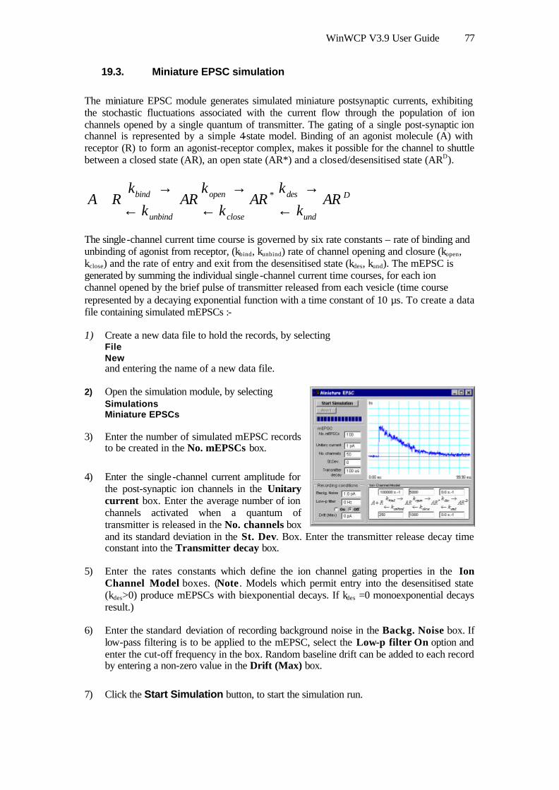
WinWCP V3.9 User Guide 77
19.3. Miniature EPSC simulation
The miniature EPSC module generates simulated miniature postsynaptic currents, exhibiting the stochastic fluctuations associated with the current flow through the population of ion channels opened by a single quantum of transmitter. The gating of a single post-synaptic ion channel is represented by a simple 4-state model. Binding of an agonist molecule (A) with receptor (R) to form an agonist-receptor complex, makes it possible for the channel to shuttle between a closed state (AR), an open state (AR*) and a closed/desensitised state (ARD).
D
und
des
close
open
unbind
bind ARk
kAR
kk
ARk
kRA
←→
←→
←→
+ *
The single-channel current time course is governed by six rate constants – rate of binding and unbinding of agonist from receptor, (kbind, kunbind) rate of channel opening and closure (kopen, kclose) and the rate of entry and exit from the desensitised state (kdes, kund). The mEPSC is generated by summing the individual single-channel current time courses, for each ion channel opened by the brief pulse of transmitter released from each vesicle (time course represented by a decaying exponential function with a time constant of 10 µs. To create a data file containing simulated mEPSCs :-
1) Create a new data file to hold the records, by selecting File New and entering the name of a new data file.
2) Open the simulation module, by selecting Simulations Miniature EPSCs
3) Enter the number of simulated mEPSC records to be created in the No. mEPSCs box.
4) Enter the single-channel current amplitude for the post-synaptic ion channels in the Unitary current box. Enter the average number of ion channels activated when a quantum of transmitter is released in the No. channels box and its standard deviation in the St. Dev. Box. Enter the transmitter release decay time constant into the Transmitter decay box.
5) Enter the rates constants which define the ion channel gating properties in the Ion Channel Model boxes. (Note . Models which permit entry into the desensitised state (kdes>0) produce mEPSCs with biexponential decays. If kdes =0 monoexponential decays result.)
6) Enter the standard deviation of recording background noise in the Backg. Noise box. If low-pass filtering is to be applied to the mEPSC, select the Low-p filter On option and enter the cut-off frequency in the box. Random baseline drift can be added to each record by entering a non-zero value in the Drift (Max) box.
7) Click the Start Simulation button, to start the simulation run.

WinWCP V3.9 User Guide 78
20. References
Brown K.M. & Dennis J.E. (1972) Derivative-free analogs of the Levenberg-Marquardt and Gauss algorithms for non-linear least squares approximation. Numerische Mathematik, 18, 289-297.
Bezanilla F. & Armstrong C. M. (1977) Inactivation of the sodium channel I. Sodium current experiments. J. Gen Physiol. 70, 548-566.
De Koninck Y & Mody I. (1994) Noise analysis of miniature IPSCs in adult rat brain slices: properties of synaptic GABAA receptor channels. J. Neurophysiol. 71, 1318-35.
Dempster J. (1986) The use of the driving function in the analysis of endplate current kinetics. J. Neurosci. Methods, 18, 277-285.
Dempster J. (1993) Computer Analysis of Electrophysiogical Signals, Academic Press, London (ISBN 0-12-208940-5)
Dempster J. (2001) The Laboratory Computer : A Guide for neuroscientists and physiologists, Academic Press.
Dilger J.P & Brett R.S. (1990) Direct measurement of the concentration- and time-dependent open probability of the nicotinic acetylcholine receptor channel. Biophys. J. 57, 723-731.
Gillis K. (1995) Techniques for membrane capacity measurements. In Single -channel recording, 2nd ed. (ed. B. Sakmann & E. Neher), Plenum Press.
McLachlan E.M. & Martin A.R. (1981) Non-linear summation of endplate potentials in the frog and mouse. J. Physiol. 311, 307-324.
Sigworth F.J. (1980) The variance of sodium current fluctuations at the node of Ranvier. J. Physiol. 307, 97-129.
Standen N.B., Gray P.T.A. & Whitaker M.J. (eds) (1987) The Plymouth Workshop Handbook, The Company of Biologists Ltd., Cambridge.
Traynelis S.F., Silver R.A. & Cull-Candy S.G. (1993) Estimated conductance of glutamate receptor channels activated during EPSCs at the cerebellar mossy fibre-granule cell synapse. Neuron 11, 279-289.

WinWCP V3.9 User Guide 79
21. Appendix: WCP data file structure.
This appendix provides a detailed specification of the internal structure of the WCP data file. The WCP data file is designed to store digitised 16 bit integer binary records of analogue signals, the associated scaling information required to reconstitute actual signal levels, validation information entered by the user, and measurements generated by WCP analysis modules.
A WCP file can contain up to 231 separate records (assuming there is sufficient disk space), each record containing up to 8 channels, and each channel containing a multiple of 256, samples, up to a total of 29952 for the whole record. (Note. All records within a file must be the same size, i.e. same number of channels and samples/channel.)
For efficiency, data is written to the file in units of 512 byte sectors. Three kinds of blocks can exist. The header block is 1024 bytes in length and contains a list of ASCII-format keywords, detailing the number of records in the file, record size, scaling factors etc. Signal records are stored in sequence after the header block, Each record consists of one 1024 byte analysis block , containing validation and analysis results pertaining to the record, followed by a data block containing the digitised A/D samples. The size of the data block is determined by the number of channels and samples/channel in the record.
For instance, a data file containing 3 records, would have the form.
H A D
Record 1
A D
Record 2
A D
Record 3
The beginning of each record can be determined (as a byte offset from the start of the file) using the formula
( ) ( )( )1024211024 / +⋅⋅−+= channelsampleschannels NNNumber RecordOffset Byte A.1
where Nchannels is the number of channels per record and Nsamples is the number of samples per record.
Header Block
The header block contains the information needed to allow a program to determine the size and number of records in the file. It is usually the first block to be read when a file is opened. File parameters are stored as ASCII text in the form of keywords, one word per line, as follows
KEY= <value> <cr> <lf>
where <value> is a number or text depending on the parameter and <cr> <lf> are the carriage return and line feed characters.

WinWCP V3.9 User Guide 80
A typical header block (from a file with 2 channels) contains the following keywords.
VER=6.4 <cr><lf> WCP version number NC=2 <cr><lf> No. of channels per record. NR=50 <cr><lf> No. of records in the file. NBH=2 <cr><lf> No. of 512 byte sectors in file header block NBA=1 <cr><lf> No. of 512 byte sectors in a record analysis block NBD=4 <cr><lf> No. of 512 byte sectors in a record data block AD=5.0000 <cr> <lf> A/D converter input voltage range (V) ADCMAX=2047 <cr><lf> Maximum A/D sample value NP=512 <cr><lf> No. of A/D samples per channel DT=.1600 <cr><lf> A/D sampling interval (s) NZ=10 <cr> <lf> No. of samples averaged to calculate a zero level. YN0=Im <cr> <lf> Channel 0 name YU0=nA <cr> <lf> Channel 0 units YS0=.146E-02 <cr> <lf> Channel 0 scale factor units/bit YG0=.167E+04 <cr> <lf> Channel 0 gain factor mV/units YZ0=1997 <cr> <lf> Channel 0 zero level (A/D bits) YO0=0 <cr> <lf> Channel 0 offset into sample group in data block YR0=2 YN1=Vm <cr> <lf> Channel 1 name YU1=mV <cr> <lf> Channel 1 units YS1=.244 <cr> <lf> Channel 1 scale factor units/bit YG1=10.0 <cr> <lf> Channel 1 gain factor mV/bit YZ1=2048 <cr> <lf> Channel 1 zero level (A/D bits) YO1=1 <cr> <lf> Channel 1 offset into sample group in data block YR1=0 <cr> <lf> TU=ms <cr> <lf> Time units ID= Cell 1 <cr> <lf> Experiment identification line
(Note that it should not be assumed that the keywords will follow any particular order)
Analysis block
The first block in each signal record is an analysis block, containing a series of internal format variables. The first 6 variables provide important classification and scaling information for the record, and are detailed as follows.
Variable Type Contents
Record status 8 x ASCII bytes ACCEPTED, REJECTED
Record type 4 x ASCII bytes TEST, LEAK, etc.
Group number 4 byte floating point
Time recorded 4 byte floating point (s)
Sampling interval 4 byte floating point (s)
Max positive limit of A/D voltage range
8 x 4 byte floating point
(1 per channel)
(V)

WinWCP V3.9 User Guide 81
The remainder of the analysis block contains the results generated for that record by the Waveform analysis and Curve fitting modules. Further details of the structure of the analysis block can be obtained by looking at the global.pas source code file.
Data block
The data block contains the digitised signals, stored in the form of 16 bit binary integers. Each A/D sample takes up 2 bytes of space. The size of the data block is determined by the number of channels and number of samples per channels in the record
N N Nbytes channels samples= ⋅ ⋅2 A.2
If there is more than one A/D input channel, samples are interleaved within the data block. For example, for 2 channels,
Y01 Y11 Y02 Y12 ..... Y0nsamples Y1nsamples A.3
Different laboratory interfaces supported by WinWCP return multi-channel A/D samples in different orders. The channel interleaving order for a data file is specified by the YOn= channel keyword in the file header block.
The calibrated signal level in the appropriate channel units can be reconstructed using information stored in the header and analysis blocks, using,
adcn
cal yYGADC
Vy
⋅=
max
max
where Vmax the maximum positive limit of the A/D converter voltage range (from analysis block) ,ADCmax is maximum A/D sample value at Vmax. (header block) and YGn is the calibration factor (Volts/channel units) for channel n (header block).