window based smart antenna design for ...airccse.org/journal/jwmn/7415ijwmn05.pdf2department of...

International Journal of Wireless & Mobile Networks (IJWMN) Vol. 7, No. 4, August 2015

DOI : 10.5121/ijwmn.2015.7405 63

WINDOW BASED SMART ANTENNA DESIGN

FOR MOBILE AD HOC NETWORK ROUTING

PROTOCOL

AKM Arifuzzman1, Rumana Islam

2, and Mohammed Tarique

3

1Department of Electrical Engineering, University of Alabama, Birmingham, AL, USA

2Department of Electrical and Electronic Engineering, American International University,

Banani, Dhaka,Bangladesh 3Department of Electrical Engineering, Ajman University of Science and Technology,

Fujairah, United Arab Emirates

ABSTRACT

Mobile Ad hoc Networks (MANETs) have drawn considerable attentions of the researchers for the last few

years. MANETs, consisting of mobile nodes, are self-organizing and self-configuring and hence can be

deployed without any infrastructure support. MANETs also have some limitations including short-life,

unreliability, scalability, latency, high interference, and limited resources. In order to overcome these

limitations many innovations and researches have been done in this field. Incorporating smart antenna

system with the mobile nodes is one of them. It has been shown in the literatures that smart antenna can

improve network capacity, increase network lifetime, reduce delay, and improve scalability by using

directional radiation pattern. But, there are some unsolved issues too. Smart antenna requires a large

number of antenna elements that a resource constraint mobile node can hardly handle. Hence, one major

design issue is to achieve a desired radiation pattern by using minimum number of antenna elements.

Another important issue is the arrangement of antenna elements. Antenna elements can be arranged in

linear, planar, and circular manners. In this paper we have addressed these issues. We have proposed a

window based smart antenna design for MANETs. Our target is to improve the routing performance of

MANETs. We have shown that by using appropriate window function a desired radiation pattern can be

achieved with a minimum number of antenna elements.

KEYWORDS

Ad hoc networks, routing protocol, DSR, smart antenna, radiation, window, energy constraint, antenna

array

1. INTRODUCTION

Wireless networking has been an active field of research since the early days of packet radio

network introduced by Defense Advanced Research Project Agency (DARPA) [1]. Recent

developments in wireless devices and applications have caused exponential growth in wireless

users. Wireless devices such as laptop computers, personal digital assistant (PDA), pagers, and

cellular phones have become portable now. Users can carry these devices anywhere at any time.

Hence, there is a need for a network that can be readily deployed at any place at any time without

any centralized administration. In many scenarios infrastructure based network is hard to build

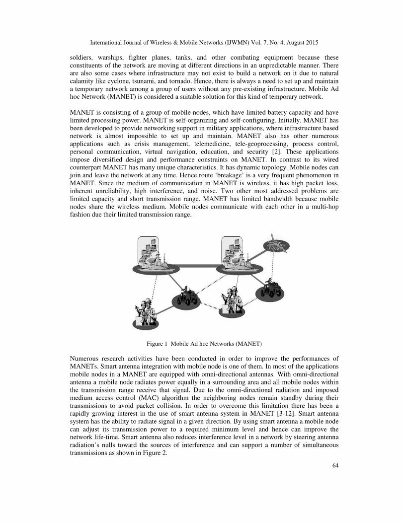
and maintain. Wireless network operating in a battlefield (see Figure 1) is an example for such

scenarios. In this scenario an infrastructure based network cannot support communication among


64

soldiers, warships, fighter planes, tanks, and other combating equipment because these

constituents of the network are moving at different directions in an unpredictable manner. There

are also some cases where infrastructure may not exist to build a network on it due to natural

calamity like cyclone, tsunami, and tornado. Hence, there is always a need to set up and maintain

a temporary network among a group of users without any pre-existing infrastructure. Mobile Ad

hoc Network (MANET) is considered a suitable solution for this kind of temporary network.

MANET is consisting of a group of mobile nodes, which have limited battery capacity and have

limited processing power. MANET is self-organizing and self-configuring. Initially, MANET has

been developed to provide networking support in military applications, where infrastructure based

network is almost impossible to set up and maintain. MANET also has other numerous

applications such as crisis management, telemedicine, tele-geoprocessing, process control,

personal communication, virtual navigation, education, and security [2]. These applications

impose diversified design and performance constraints on MANET. In contrast to its wired

counterpart MANET has many unique characteristics. It has dynamic topology. Mobile nodes can

join and leave the network at any time. Hence route ‘breakage’ is a very frequent phenomenon in

MANET. Since the medium of communication in MANET is wireless, it has high packet loss,

inherent unreliability, high interference, and noise. Two other most addressed problems are

limited capacity and short transmission range. MANET has limited bandwidth because mobile

nodes share the wireless medium. Mobile nodes communicate with each other in a multi-hop

fashion due their limited transmission range.

Figure 1 Mobile Ad hoc Networks (MANET)

Numerous research activities have been conducted in order to improve the performances of

MANETs. Smart antenna integration with mobile node is one of them. In most of the applications

mobile nodes in a MANET are equipped with omni-directional antennas. With omni-directional

antenna a mobile node radiates power equally in a surrounding area and all mobile nodes within

the transmission range receive that signal. Due to the omni-directional radiation and imposed

medium access control (MAC) algorithm the neighboring nodes remain standby during their

transmissions to avoid packet collision. In order to overcome this limitation there has been a

rapidly growing interest in the use of smart antenna system in MANET [3-12]. Smart antenna

system has the ability to radiate signal in a given direction. By using smart antenna a mobile node

can adjust its transmission power to a required minimum level and hence can improve the

network life-time. Smart antenna also reduces interference level in a network by steering antenna

radiation’s nulls toward the sources of interference and can support a number of simultaneous

transmissions as shown in Figure 2.


65

There are also other advantages of using smart antenna in MANET. These advantages are

addressed in [16]. In this paper we limit our effort only to investigate the effects of smart antenna

on the routing protocol of MANET. There are many routing protocols have been proposed for

MANET. Among these protocols Dynamic Source Routing (DSR) protocol is a popular one [17].

In this paper we propose a smart antenna system for MANET to improve the performance of the

DSR routing protocol. The rest of the paper is organized as follows. Section 2 presents a brief

introduction to smart antenna. Section 3 presents the basic operation of DSR protocol. The effects

of smart antenna on the routing protocol have been described in section 4. Section 5 contains the

smart antenna design issues for MANET. Section 6 introduces window functions and section 7

describes the side lobe minimization techniques by using window functions. The design trade-offs

have been discussed in section 8. This paper is concluded with section 9.

Figure 2 Capacity improvement of ad hoc network with smart antenna [10]

2. SMART ANTENNA

Smart antennas are composed of a collection of two or more antenna elements called antenna

array. These antenna elements work together to establish a unique radiation pattern in a desired

direction. A functional block diagram of a smart antenna system is shown in Figure 3. It is

depicted in the figure that digital signal processor is the backbone of such system. Smart antenna

system can locate and track desired signal called Signal of Interest (SOI) and also Signal of no

Interest (SNOI). The smart antenna system can dynamically adjust the radiation of the antenna

elements so that the resultant radiation is directed along the SOI and it can suppress the radiation

pattern along the direction of SNOIs. In order to track the radiation pattern direction of arrival

(DOA) or angle of arrival (AOA) algorithms is used. The DOA algorithm helps the antenna

elements to set the desired excitation weights in terms of magnitude and phase so that the

radiation can be directed in a desired direction.

Figure 3 Smart antenna system


66

Antenna array can be arranged in many different ways. Most popular arrangements are linear

array, circular array, and planer arrays. These arrangements are associated with different level of

complexity in terms of hardware and software. Since mobile nodes in ad hoc networks are

constrained with limited processing power and limited battery life, it is imperative to choose a

suitable arrangement. In this paper we focus on two main issues. First, we have investigated

different types of antenna arrangement for the mobile nodes so that the required radiation pattern

can be achieved with minimum complexity. Second, we have investigated the required number of

antenna elements for each type of arrangement. With too few antennas desired radiation pattern

cannot be achieved. On the other hand too many antennas should not be selected for resource

constraint mobile nodes. In this paper we investigate these issues so that an optimum number of

antennas can be arranged in a proper arrangement and the performance of DSR routing protocol

can be improved.

3. DYNAMIC SOURCE ROUTING PROTOCOL

The DSR protocol is an on-demand reactive routing protocol [17]. It consists of two main

mechanisms namely (a) route discovery, and (b) route maintenance.

Route discovery is a mechanism by which a source node finds a route to a destination. If a source

node wants to send some packets to a destination, it first searches its route cache to find a route. If

the source node cannot find a route there, it initiates the route discovery process by transmitting a

route request message. Each route request contains unique route request ID in addition to the

source and destination addresses. All other nodes, within the range of the source, receive the

request message. These nodes check the destination address of the request message. If the

destination address does not match with the node’s own address, it appends its address in the

route request and re-broadcast the message. This process goes on unless the route request reaches

its intended destination. Once the desired destination node receives the route request, it sends a

reply packet to the source. The destination node copies the accumulated routing information from

the route request packet to the route reply packet. When the source node receives the route reply

packet, it records the newly discovered route in its route cache and starts sending data packet via

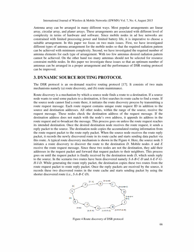
this route. A typical route discovery mechanism is shown in the Figure 4. Here, the source node S

initiates a route discovery to discover the route to the destination D. Mobile nodes A and E

receive the route request message. Since these two nodes are not the destination, they add their

addresses in the request packet and forward that request packets to their neighbors. This process

goes on until the request packet is finally received by the destination node D, which sends reply

to the source. In the scenario two routes have been discovered namely S-A-B-C-D and A-E-F-G-

H-I-D. While generating the route reply packet, the destination copies these two routes from the

route request packet to route reply packet. Once the reply packets are received by the source, it

records these two discovered routes in the route cache and starts sending packet by using the

shorter discovered route (i.e., S-A-B-C-D).

Figure 4 Route discovery of DSR protocol


67

Route maintenance mechanism helps a mobile node to detect changes in the network topology. If

a node cannot send a packet to the destination due to ‘broken’ link, it initiates the route

maintenance mechanism. By using this mechanism a mobile node sends a message to the source

node (and other nodes on the same route) about the ‘broken’ link. The DSR protocol uses

acknowledgment mechanism of the underlying Medium Access Control (MAC) protocol for the

‘broken’ link detection. For example, IEEE 802.11 Wireless LAN medium access layer provides

acknowledgement for each packet. If the transmitting node does not receive any

acknowledgement after sending a packet several times through a link, it treats that link as

‘broken’ and updates its route cache by marking the route as ‘invalid’. A typical route

maintenance mechanism is illustrated in Figure 5. In this scenario it is assumed that mobile C

exhausts battery and hence the link B-C is ‘broken’. Node B tries to send packets to C for several

times and node C sends no acknowledgement packet. The node B assumes that the link B-C is

broken. In order to let the source S and other nodes (i.e., B and A) lying on the same route, mobile

node B generates a route error message and sends it to these nodes. Once route error message is

received by the source S, it marks the route S-A-B-C-D invalid in the route cache and starts

sending data packets by using the other alternative route (i.e., A-E-F-G-H-I-D).

Figure 5 Route maintenance mechanism of DSR protocol

4. DSR PROTOCOL IMPROVEMENT BY SMART ANTENNA

The route request mechanism of DSR routing protocol can be made more efficient by using smart

antenna. In DSR, a node can learn and cache multiple routes to a destination by means of a single

route discovery. To ensure this multiple routing strategy work all neighboring nodes are obligated

to re-broadcast once they receive a route request. The ultimate outcome of the re-broadcasting is

’flooding’ of overhead packets in the network. Although some measures have been adopted in the

DSR protocol to reduce flooding such as limiting the rate of route discovery by using random

back-off algorithm, and imposing shorter hop count (’ring zero search’ mechanism); flooding

problem is still severe in the DSR protocol specially for a large network. Some of the drawbacks

related to flooding are redundant re-broadcast, contention, and collision.

Figure 6 Broadcast reduction


68

The redundant broadcast occurs when a mobile node re-broadcasts a route request message to its

neighbors, which may have already received that message from other nodes. The contention

problem occurs when all neighbors of a node re-broadcast the request packet at the same time.

These neighbors may severely contend with each other to get access to the medium. The

collisions are more likely to occur when all neighboring nodes try to re-broadcast at the same

time. Such kind of broadcasting is illustrated in Figure 6. In this scenario node A is the source and

node D is the destination. When node A initiates the route discovery mechanism by broadcasting

the route request packet, all the neighboring nodes namely B, C, and G receive the request packet

and re-broadcast. Hence, there will be six copies of the request messages in the network. This

type of redundant message can be easily reduced by using smart antenna. Let us assume that node

G, equipped with smart antenna, can determine the angle of arrival (AOA) of the request message

once it receives from the source node A. Hence, node G should broadcast in a direction that is in

opposite of arrival direction estimated from the received request message. Finally, the destination

node receives the request packet broadcast by the node G and hence sends reply back to the

source A. The reply packet carries the information about the route A-G-D.

Smart antenna can also help to efficiently handle route reply packet. For example when the node

D generates a route reply packet, it sends the packet through the route D-G-A. Since the node D

and G already know the direction of the arrivals (DOAs) from the route requests, these nodes

should send the reply packet in a desired direction. Hence, the route reply packets are not going to

affect the other nodes (i.e., E,F,B, and C) transmissions; and these nodes can perform their normal

network operation.

Figure 7 Data packet delivery

Once a route is discovered a source node starts sending data packet by using the discovered route.

This kind of data packet delivery is illustrated in Figure 7. In this scenario node A is the source of

the data packet. Node C is the destination node and node B is a forwarding node (i.e., router).

Since the AOAs are known from the route reply packet, node A adjusts its antenna elements’

weights accordingly. Hence, the resultant radiation pattern’s main lobe will be directed toward

node B. The node B also adjusts the weights of the antenna elements so that it can direct the

radiation pattern toward node C. Since all the nodes involved in the data transmission have

appropriately adjusted the antennas weights, their transmissions will not affects other surrounding

nodes.

The smart antenna also helps in handling the route error message. Assume that the link between

node B and C is ‘broken’ for some reason. The node B generates a route error message and sends

it to node A to let it know that the route B-C is broken. While sending the route error message

node B radiates the signal in the desired direction so that other nodes are not affected.


69

Although smart antenna system helps the MANETs to improve the routing performance as

discussed above, it has some drawbacks too. One of the drawbacks is that mobile nodes should be

equipped with transceivers that are much more complex than traditional transceiver. Determining

the necessary weights for antenna elements is also computationally extensive and hence a very

powerful processor needs to be associated with the mobile nodes. Moreover, mobile nodes should

minimize the side lobes. Although the smart antenna helps the mobile nodes to direct main

radiation lobe in a desired direction, there is always a chance of generating additional minor lobes

as shown in Figure 7. One of the solutions for minimizing the minor lobes is to increase the

number of antenna elements. This may not always be feasible because of the high cost and

complexity associated with the increasing number of antenna elements. Hence, the main design

objective will be to have a desired radiation pattern with the minimum number of antenna

elements. Moreover, the antenna arrangement should be as simple as possible so that it can be

easily equipped with the nodes.

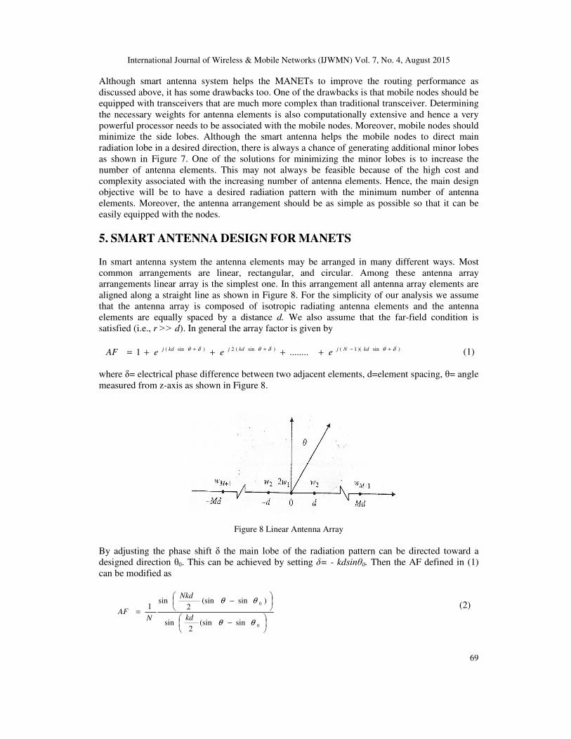
5. SMART ANTENNA DESIGN FOR MANETS

In smart antenna system the antenna elements may be arranged in many different ways. Most

common arrangements are linear, rectangular, and circular. Among these antenna array

arrangements linear array is the simplest one. In this arrangement all antenna array elements are

aligned along a straight line as shown in Figure 8. For the simplicity of our analysis we assume

that the antenna array is composed of isotropic radiating antenna elements and the antenna

elements are equally spaced by a distance d. We also assume that the far-field condition is

satisfied (i.e., r ˃˃ d). In general the array factor is given by

)sin)(1()sin(2)sin( ........1 δθδθδθ +−++ ++++= kdNjkdjkdj

eeeAF (1)

where δ= electrical phase difference between two adjacent elements, d=element spacing, θ= angle

measured from z-axis as shown in Figure 8.

Figure 8 Linear Antenna Array

By adjusting the phase shift δ the main lobe of the radiation pattern can be directed toward a

designed direction θ0. This can be achieved by setting δ= - kdsinθ0. Then the AF defined in (1)

can be modified as

−

−

=

0

0

sin(sin2

sin

)sin(sin2

sin1

θθ

θθ

kd

Nkd

NAF

(2)


70

A plot of the array factor for different antenna array size is illustrated in Figure 9. In this antenna

array the phase shifts of the antenna elements have been adjusted to have a radiation pattern with

main lobe directed toward θ0=30o. It is depicted in this figure that the beam width of the main

lobe is reduced with the number of elements (i.e., N) in the antenna array.

−90 −60 −30 0 30 60 900

0.1

0.2

0.3

0.4

0.5

0.6

0.7

0.8

0.9

1

θ

AF

N=4

N=8

N=16

Figure 9 Array factor for a linear antenna array

Although linear array draws considerable attention for its simplicity in design, it is not considered

suitable when mounted on the mobile nodes. Other arrangement like circular array is considered

an alternative of linear array. Figure 10 shows the arrangement of circular antenna arrays. The

antennas are located at the radius a as shown in the figure. The phase angle of the nth antenna

element is denoted by φn . The array factor of circular array is defined as

∑=

+−−=N

n

kaj nneAF1

])cos(sin[ δφφθ (3)

,where a=radius of the circular path, δn=phase angle of the nth antenna element. The plot of array

factors for a typical circular antenna array is shown in Figure 11. In this array the antenna

elements are placed on a circle of radius a=1λ, the size of the antenna array was varied from N=4

to N=16, and the radiation pattern was directed toward θ0=300. It is depicted in the figure that

circular array shows larger side lobes compared to that of linear array for the same number of

antenna elements. For the smallest array size (i.e., N=4) the side lobes are even equal to that of

the main lobe.

Figure 10 Circular Antenna Array


71

−90 −60 −30 0 30 60 900

0.1

0.2

0.3

0.4

0.5

0.6

0.7

0.8

0.9

1

θ

AF

Circular Array elements, radius=1λ

N=4

N=8

N=16

Figure 11 Array factor for circular array

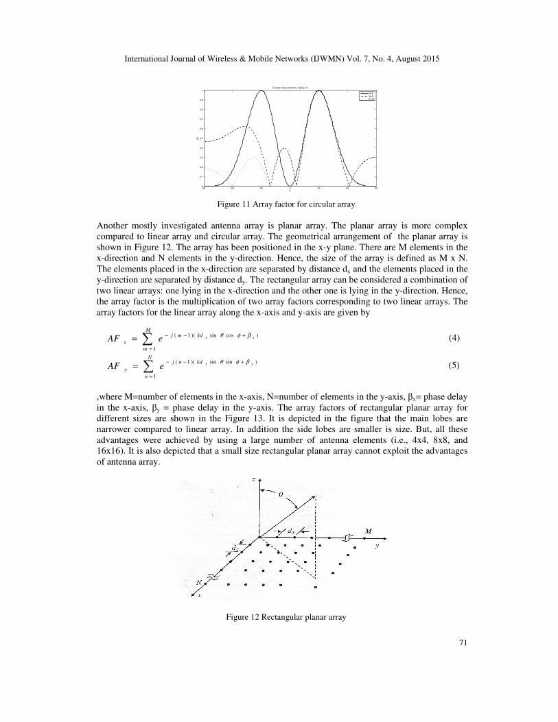
Another mostly investigated antenna array is planar array. The planar array is more complex

compared to linear array and circular array. The geometrical arrangement of the planar array is

shown in Figure 12. The array has been positioned in the x-y plane. There are M elements in the

x-direction and N elements in the y-direction. Hence, the size of the array is defined as M x N.

The elements placed in the x-direction are separated by distance dx and the elements placed in the

y-direction are separated by distance dy. The rectangular array can be considered a combination of

two linear arrays: one lying in the x-direction and the other one is lying in the y-direction. Hence,

the array factor is the multiplication of two array factors corresponding to two linear arrays. The

array factors for the linear array along the x-axis and y-axis are given by

∑=

+−−=M

m

kdmj

xxxeAF

1

)cossin)(1( βφθ (4)

∑=

+−−=

N

n

kdnj

y

yyeAF1

)sinsin)(1( βφθ (5)

,where M=number of elements in the x-axis, N=number of elements in the y-axis, βx= phase delay

in the x-axis, βy = phase delay in the y-axis. The array factors of rectangular planar array for

different sizes are shown in the Figure 13. It is depicted in the figure that the main lobes are

narrower compared to linear array. In addition the side lobes are smaller is size. But, all these

advantages were achieved by using a large number of antenna elements (i.e., 4x4, 8x8, and

16x16). It is also depicted that a small size rectangular planar array cannot exploit the advantages

of antenna array.

Figure 12 Rectangular planar array


72

−90 −60 −30 0 30 60 900

0.1

0.2

0.3

0.4

0.5

0.6

0.7

0.8

0.9

1

θ

AF

Rectangular Planar Array with, dx=dy=1λ

N=4

N=8

N=16

Figure 13 Array factor for rectangular planar array

6. THE WINDOW FUNCTIONS FOR SIDE LOBE MINIMIZATION

In the analyses of the different antenna array arrangements above we assume that all the antenna

elements are isotropic in nature and all have unity amplitude. It was depicted in Figure 9, Figure

11, and Figure 13 that all the array factors have side lobes. In other words the antenna array

elements not only radiate power in an intended direction, but also they radiate power in

unintended directions. These unintended radiations may affect other mobile nodes’ transmissions.

Hence, it is imperative that these side lobes should be minimized as much as possible.

Table 1 Window functions

Name of Window Time-domain sequence, 0 ≤ n ≤ M-1

Binomial Coefficients of :

.....!2

)2)(1()1()( 2)3(211 +

−−+−+=+ −−−−

baMM

baMabaMMMM

Blackman 1

4cos08.0

1

2cos5.045.0

−+

−−

M

n

M

n ππ

Gaussian 2

2/2

1

−

N

n

eα

,α=2.5

Hamming 1

2cos46.054.0

−−

M

nπ

Kaiser

−

−−−

−

2

1

2

1

2

1

0

22

0

MI

Mn

MI

α

α, α=0.5

Chebysev

( )[ ]β

πβ

1

1

coshcosh

coscoscosh

−

−

M

M

kM

k=0,1,2……(M-1)

( )[ ]ββ

1

01

coshcosh

)10(cosh1

cosh

−

−

=M

M α=2,3,4


73

Figure 14 Windows and their spectrums

1 2 3 4 5 6 7 8 90

10

20

30

40

50

60

70

n

h(n)

0 0.2 0.4 0.6 0.8 1−800

−700

−600

−500

−400

−300

−200

−100

0

normalized frequency (x pi)

Mag

nitu

de (d

B)

(a) Binomial window

1 2 3 4 5 6 7 8 90

0.1

0.2

0.3

0.4

0.5

0.6

0.7

0.8

0.9

1

n

h(n)

0 0.2 0.4 0.6 0.8 1−450

−400

−350

−300

−250

−200

−150

−100

−50

0


Mag

nitu

de (d

B)

(b) Blackman window

1 2 3 4 5 6 7 8 90

0.1

0.2

0.3

0.4

0.5

0.6

0.7

0.8

0.9

1

n

h(n)

0 0.2 0.4 0.6 0.8 1−150

−100

−50

0


Mag

nitu

de (d

B)

(c) Gaussian Window

1 2 3 4 5 6 7 8 90

0.1

0.2

0.3

0.4

0.5

0.6

0.7

0.8

0.9

1

n

h(n)

0 0.2 0.4 0.6 0.8 1−140

−120

−100

−80

−60

−40

−20

0


Mag

nitu

de (d

B)

(d) Hamming Window

1 2 3 4 5 6 7 8 90

0.1

0.2

0.3

0.4

0.5

0.6

0.7

0.8

0.9

1

n

h(n)

0 0.2 0.4 0.6 0.8 1−120

−100

−80

−60

−40

−20

0


Mag

nitu

de (d

B)

(e) Kaiser Window

(f) Chebysev Window


74

(a)

(b)

(c)

Figure 15 Linear array patterns for (a) N=8, (b) N=16, and (c) N=32

There have been many proposals to minimize the side lobes. In this work we consider window

functions. A number of window functions can be found in the literatures [14-15]. In this paper we

consider some popular window functions namely Binomial, Blackman, Gaussian, Hamming,

Kaiser, and Chebysev. Among these window functions Binomial and Chebysev have drawn

considerable attentions in the field of antenna array design. The other window functions have

been extensively used in digital signal processing. We consider these window functions for


75

designing smart antenna for MANETs. Our prime objective is to minimize the side lobes by using

a minimum number of antenna elements. Table 1 lists these window functions and Figure 14

illustrates the time-domain and frequency domain characteristics of the window functions.

The Binomial window is generated by using Pascal’s triangle. The frequency domain

characteristics of Binomial window show some minor side lobes. It is shown in Figure 14(a) that

the minor lobes of binomial window are far below the main side lobe. The Blackman window

also exhibits some side lobes. The first side lobe occurs at -100 dB below the main side lobe as

shown in Figure 14(b). But, there are some other visible side lobes that have similar magnitude

compared to other side lobes. The frequency characteristic of the Gaussian window is similar to

that of Blackman window. In both cases the first side lobe occurs around -60 dB below the main

lobe. The Hamming window is another popular window. In this window function the first side

lobe occurs around -45 dB below the magnitude of the main lobe. The Kaiser window behaves

differently compared to other window functions. But, the Kaiser window also produces some side

lobes, which decay quickly. Another popular window is the Chebysev window. It is shown in the

figure that the Chebysev window produces some side lobes. But the magnitude of these side lobes

is far below the magnitude of the main lobe. Considering transition of the main lobe of the Kaiser

window shows a steeper transition compared to other window functions. The transition of the

Hamming window is slightly slower than the Kaiser window, but it is faster than the Gaussian,

Binomial, and Blackman window. Although the Binomial window does not show any side lobe

it’s transition bandwidth is the slowest one.

7. MINIMIZING SIDE LOBES

We consider again the three antenna arrangements as discussed in section 5. But, the excitation

amplitudes of the antenna elements are now varied according to the window functions. In all

cases the desired maximum radiation is θ=00. The plot of the array factor for linear array

consisting of different number of antenna elements is shown in Figure 15. In this figure it is

depicted that the desired angle of the radiation pattern is θ=00. But, the beam width becomes

narrower with the increase in the number of elements. The beam width also varies with the

window types. This figure shows that the Kaiser window provides the narrowest beam width. For

example, the Half Power Beam Width (HPBW) for antenna array with four elements is 300 for the

Kaiser window. But, the same is 150 and 70 for antenna elements eight and sixteen. The problem

of the Kaiser window based linear array is that there exists some side lobes. The side lobe can be

minimized by other window like the Chebysev window. It is depicted in the figure that the

Chebysev window does not show any side lobe. But it shows a much higher HPBW (i.e.,540) than

the Kaiser window. Hence, an antenna array consisting of four elements the Chebysev window

will be chosen. For antenna arrays consisting of eight elements and sixteen elements the

Hamming window provides the narrowest HPBW and the minimum side lobes.

The radiation patterns for planar array are shown in Figure 16. For planar array with antenna

elements 4x4 is shown in Figure 16(a). Compared to linear array (see Figure 15(a)) planar array

has the same HPBW. But, all windows show side lobes. Hence, planar array with 4x4 antenna

elements may not be considered suitable for antenna elements. Planar antenna arrays with 8x8

elements and 16x16 elements show narrower HPBWs. Although there are some side lobes exist in

these cases, their magnitudes are not significant.


76

(a)

(b)

(c)

Figure 16 Planar array elements (a)4x4, (b) 8x8, and (c) 16x16

The radiation patterns for a circular array are shown in Figure 17. Although the circular antenna

arrays have some advantages over linear array, its radiation pattern is not desirable. For example,

the HPBW for circular array with 4 antennas are similar to those of linear and planar array. But,

the side lobes have equal magnitude compared to the main lobe. The side lobes are minimized by

increasing the number of elements as shown in Figure 17 (b) and 17 (c). Still, the HPBW does not

narrow down like that of the linear and planar arrays. Considering the radiation patterns we

conclude that circular array is not a good candidate for antenna array.


77

(a)

(b)

(c)

Figure 17 Circular array with antenna elements N=8, N=16, and N=32


78

8. THE DESIGN TRADE-OFFS IN MANETS

Since the mobile nodes in MANETs have very limited processing power and battery power, we

need to be very careful about selecting appropriate antenna array for them. Keeping these

constraints in mind antenna array for MANETs should be designed with a minimum number of

antenna elements. But, we have shown in Section 5 that the HPBW depends on the number of

antenna elements. The more the number of elements, the narrower is the bandwidth. Hence, the

desired design objective will be to select the minimum number of antenna elements at the same

time to maintain the desired radiation pattern.

Among the three antenna arrays the linear antenna array provides the least flexibility. The linear

antenna array allows radiation pattern to vary only in the θ direction only. We also notice that

linear antenna array consisting of 16 antenna elements provides a very narrow HPBW. On the

other hand, antenna array with 4 elements provides a very large HPBW. It has been shown in the

literature that the performances of ad hoc network highly depend on the network density. In a

highly dense network the interference level will be high and vice versa. Hence, we need to

maintain a very narrow HPBW in a dense network and we need to equip the mobile nodes with a

large number of antenna elements in a dense network. There is another problem too. Mobile node

should have a high processing power to handle a large number of antenna elements. In this regard

linear antenna array consisting of 16 antenna elements will be a good candidate. While selecting

windows for minimization of the side lobes either the Kaiser window or the Hamming window

can be used for such case. The Kaiser window provides the narrowest HPBW, but it shows some

side lobes as shown in Figure 15(c). On the other hand the Hamming window provides a little bit

higher HPBW, but it shows no side lobes.

On the other hand, a linear antenna array consisting of 4 elements may be good enough for a low

density network to provide a moderate HPBM. Mobile nodes with low processing power will be

good enough to handle these few antenna elements. Regarding the side lobe minimization the

Kaiser window and the Chebysev window will the suitable ones. Again, the Kaiser window

exhibits the narrowest HPBW, but it shows some side lobes. On the other hand the Chebysev

window exhibits higher HPBW compared to the Kaiser window, but it exhibits no side lobe.

The rectangular ( or planar) array provides more flexibility in controlling the radiation patter. In

contrast to linear array rectangular antenna array allows the radiation pattern to vary both in θ and

ϕ direction. The major limitation of the rectangular array is the complexity. A complex algorithm

is used to set the magnitude and phase of the antenna elements. Another limitation is associated

with the large number of antenna elements that are required to have a very narrow beam width for

a dense network. It is shown in Figure 16 that an antenna array consisting of 256 elements (i.e.

16x16) provides a very narrow beam width, but it shows some side lobe irrespective of the

window function used. It is very difficult to equip a mobile node with 256 antenna elements to

achieve the desired radiation pattern. There will be similar complexity associated with antenna

array consisting of 64 elements. Only suitable candidate for ad hoc network is 4x4 rectangular

antenna array. But, this antenna array has two major limitations. One limitation is that it has a

large HPBW as shown in Figure 16(a). The other limitation is the side lobes. Irrespective of

window function used this antenna array always shows some side lobes.

Similar to rectangular antenna array circular array provides more flexibility compared to linear

array. It allows the radiation pattern to vary both in θ and ϕ direction. The other advantage of

circular antenna array is associated with its compact size as mentioned in earlier section. But, the

major limitation of the circular array is that it does not provide a very narrow beam width. A very

large antenna array even does not provide a very narrow beam width as shown in Figure 16.

Hence, circular antenna array should be avoided in MANETs.


79

9. CONCLUSION

In this paper smart antenna design for MANETs has been addressed. Smart antenna design for

MANETs is not a very straight forward because the mobile nodes have very limited processing

power. Hence, smart antenna in ad hoc network should be very simple in architecture and also

should be consisting of limited number of antenna elements. It is shown in this paper that a large

antenna array is required for a densely populated MANETs to have a very narrow beam width.

So, we should be very careful about using smart antenna in a dense network. Smart antenna can

be used in a low density network because a small number of antenna elements can provide

necessary beam width. It is also shown in this paper that linear antenna array is the best choice for

an ad hoc network. By using appropriate window function a linear antenna array consisting of 8

elements is a good candidate for a low density network. A linear antenna array consisting of 16

elements may also be used in a dense network. The rectangular antenna array and circular antenna

array will be avoided in MANETs due to their associated complexity.

REFERENCES

[1] Jubin, J. and Torrow, J. ” The DARPA Packet Radio Network Protocol”, Proceedings of the IEEE,

Vol. 75, No. 1, January 1987, pp. 21-32

[2] Goldsmith, A.J. and Wicker, S.B., “Design challenges for energy-constrained ad hoc wireless

networks”, IEEE Wireless Communication”, Vol. 9, No. 4, August, 2002, pp. 8-27

[3] Bellofiore, S., Foutz, J., Govinfarajula, R., Bachceci, I., Balanis, C.A., Spanais, A.S., Capone J.M.,

and Duman, T.M., “ Smart antenna system analysis, integration, and performance for mobile ad hoc

networks (MANETs)”, IEEE Transaction on Antennas and Propagation, Vol. 50, No. 5, May 2002,

pp. 571-581

[4] Radhakrishnan, R., Lai, D., Caffery, J., and Agrawal, D.P.,” Performance comparison of smart

antenna techniques for spatial multiplexing in ad hoc networks”, Proceedings of the 5th International

Symposium on Wireless Personal Multimedia Communications, 2002, Vol. 1, 2002, pp. 168-171

[5] Nasipuri, A., Ye S., You J, and Hiromoto, “ A MAC protocol for mobile ad hoc networks

usingdirectional antennas”, Proceedings of IEEE Wireless Communication and Networking

Conference, Chicago, IL, 2000, Vol. 3, pp. 1214 – 1219

[6] Takai, M., Martin, J., Bagrodia R., and Ren A, “ Directional Virtual Carrier Sensing for Directional

Antennas in Mobile Ad hoc Networks”, Proceedings of the 3rd ACM international symposium on

Mobile ad hoc networking & computing, Lausanne, Switzerland, June 2002, pp.183-193

[7] Roychoudhury R., Yang X., Ramanathan R., and Vaidya N., “ Medium Access Control in Ad hoc

Networks Using Directional Antenna”, Proceedings of the 8th Annual International Conference on

Mobile Computing and networking, Atlanta, Georgia, September 2002

[8] Bao L., and Garcia-Luna-Aceves, “ Transmission Scheduling in Ad hoc Networks with Directional

Antenna”, Proceedings of the 8th Annual International Conference on Mobile Computing and

networking, Atlanta, Georgia, September 2002,pp. 48-58

[9] Spyropoulos A., and Raghabendra, “ Capacity Bounds for Ad hoc Network using Directional

Antennas”, Proceedings of the IEEE International Conference on Communication, Anchorage,

Alaska, May 2003, Vol. 1, pp. 348-352

[10] Ramanthan R, “ On the Performance of Beamforming Antennas in Ad Hoc Networks”, Proceedings

of the ACM Symposium on Mobile Ad Hoc Networking & Computing, Long Beach, CA, October

2001, pp. 95-105

[11] Spyropoulos A., and Raghavendra C.S., “ Energy Efficient Communications in Ad hoc Networks

Using Directional Antennas”, Proceedings of the 22nd Annual Joint Conference of the IEEE

Computer and Communications Societies, San Francisco, CA, March-April, 2003, Vol. 1, pp. 220-

228

[12] Nasipuri A., Li K, and Sappidi U.R., “ Power Consumption and Throughput in Mobile Ad hoc

Networks using Directional Antennas”, Proceedings of the 11th Conference on Computer

Communication and Networks, Miami, FL, October 2002, pp. 620-626


80

[13] Constantine A. Belanis, “ Antenna Theory: Design and Analysis”, The 3rd Edition, John Wiley and

Sons, NJ, pp. 978-979

[14] Fredric J. Harris, “ On the use of Windows for Harmonic Analysis with the Discrete Fourier

Transform”, Proceedings of IEEE, Vol. 66, 1978, pp. 51-83

[15] Alber H. Nuttal, “ Some Windows with Very Good Sidelobe Behavior”, IEEE Transactions on

Acoustics, Speech, and Signal Processing, Vol. 29, No. 1, February 1981, pp. 84-91

[16] Winters, J.H. ; Eigent Technol., Holmdel, NJ, “ Smart antenna techniques and their applications to

Wireless Ad hoc networks”, IEEE Wireless Communication, Vol. 3, No. 4, August 2006, pp. 77- 83

[17] The Dynamic Source Routing (DSR) Protocol for Mobile Ad hoc Networks for IPV4 available at

https://www.ietf.org/rfc/rfc4728.txt

window based smart antenna design for ...airccse.org/journal/jwmn/7415ijwmn05.pdf2department of...

Documents