Wind Resource Mapping in Papua New Guinea

MESOSCALE MODELING REPORT AUGUST 2015

This report was prepared by DTU Vindenergi and 3E, under contract to The World Bank.

It is one of several outputs from the wind Resource Mapping and Geospatial Planning Papua New Guinea [Project ID: P145864]. This activity is funded and supported by the Energy Sector Management Assistance Program (ESMAP), a multi-donor trust fund administered by The World Bank, under a global initiative on Renewable Energy Resource Mapping. Further details on the initiative can be obtained from the ESMAP website. This document is an interim output from the above-mentioned project. Users are strongly advised to exercise caution when utilizing the information and data contained, as this has not been subject to full peer review. The final, validated, peer reviewed output from this project will be the Papua New Guinea Wind Atlas, which will be published once the project is completed.

Copyright © 2015 International Bank for Reconstruction and Development / THE WORLD BANK

Washington DC 20433

Telephone: +1-202-473-1000

Internet: www.worldbank.org

This work is a product of the consultants listed, and not of World Bank staff. The findings, interpretations,

and conclusions expressed in this work do not necessarily reflect the views of The World Bank, its Board of

Executive Directors, or the governments they represent.

The World Bank does not guarantee the accuracy of the data included in this work and accept no

responsibility for any consequence of their use. The boundaries, colors, denominations, and other

information shown on any map in this work do not imply any judgment on the part of The World Bank

concerning the legal status of any territory or the endorsement or acceptance of such boundaries.

The material in this work is subject to copyright. Because The World Bank encourages dissemination of its

knowledge, this work may be reproduced, in whole or in part, for non-commercial purposes as long as full

attribution to this work is given. Any queries on rights and licenses, including subsidiary rights, should be

addressed to World Bank Publications, The World Bank Group, 1818 H Street NW, Washington, DC 20433,

USA; fax: +1-202-522-2625; e-mail: pubrights@worldbank.org. Furthermore, the ESMAP Program Manager

would appreciate receiving a copy of the publication that uses this publication for its source sent in care of

the address above, or to esmap@worldbank.org.

info@3E.eu

www.3E.eu

3E nv/sa

Kalkkaai 6 Quai à la Chaux

B-1000 Brussels

T +32 2 217 58 68

F +32 2 219 79 89

Fortis Bank 230-0028290-83

IBAN: BE14 2300 0282 9083

SWIFT/BIC: GEBABEBB

RPR Brussels

VAT BE 0465 755 594

WIND RESOURCE MAPPING FOR PAPUA NEW

GUINEA

INTERIM OUTPUT - MESOSCALE MODELLING REPORT

Client: International Bank for Reconstruction and Development

(member of the World Bank Group)

Contact Person: Gerard Fae, Oliver Knight

3E Reference: PR107654.D1.2.v2

3E Contact Person: Rory Donnelly

Date: 11/08/2015

Version: Final version

Classification: Confidential

info@3E.eu

www.3E.eu

3E nv/sa

Kalkkaai 6 quai à la chaux

B-1000 Brussels

T +32 2 217 58 68

F +32 2 219 79 89

Fortis Bank 230-0028290-83

IBAN: BE14 2300 0282 9083

SWIFT/BIC: GEBABEBB

RPR Brussels

VAT BE 0465 755 594

1 INTRODUCTION & DISCLAIMER

The “Renewable Energy Resource Mapping – Wind Papua New Guinea, East Asia Pacific Region”

activity is one of several country projects funded and supported by the Energy Sector Management

Assistance Program (ESMAP) under a global initiative on Renewable Energy Resource Mapping.

This document is an interim output from the above-mentioned World Bank project and outlines the

preliminary mesoscale modelling results obtained in Phase 1 (Preliminary modelling and

implementation planning) of the project.

The report by the Department of Wind Energy of the Danish Technological University (DTU) is

contained as an annex to this report.

This document is based on an agreement entered into between the International Bank for

Reconstruction and Development (“Client”) and 3E, and is intended for the sole use of Client, and no

third-party beneficiaries are created hereby. To the extent permitted by law, 3E will not be liable

(whether in contract, tort including without limitation negligence, or otherwise) to third parties.

This document has been prepared in good faith on the basis of information available at the date of

publication without any independent verification. 3E does not guarantee or warrant the accuracy,

reliability, completeness or currency of the information in this document nor its usefulness in achieving

any purpose. Readers are responsible for assessing the relevance and accuracy of the content of this

document. 3E will not be liable for any loss, damage, cost or expense incurred or arising by reason of

any person using or relying on information in this document.

This document is protected by copyright and may only be reproduced and circulated in accordance with

the associated conditions stipulated in 3E’s written agreement with Client. No part of this document

may be disclosed in any public offering memorandum, prospectus or stock exchange listing, circular or

announcement without the express and prior written consent of 3E. The fact that Client is permitted to

redistribute this document shall not thereby imply that 3E has any liability to any recipient other than

Client.

2 OBJECTIVES

The objective of this report is to describe the modelling strategy and method, show the output of the

preliminary model results, and describe how these compare with a selection of existing measurement

datasets.

Wind Resource Mapping for Papua New Guinea

Interim output - Mesoscale modelling report

PR107654 – 11/08/2015

FINAL VERSION

CONFIDENTIAL

3 / 5

3 METHODOLOGY

The methodology employed is the use of the Weather Research and Forecasting (WRF) model, driven

by Climate Forecast System Reanalysis (CFSR) data at a resolution in the inner domain of 5 km. This

inner domain covers the entirety of Papua New Guinea. The WRF model was run in a series of

overlapping 11 day long simulations, run in parallel. The first 24 hours of each has been discarded to

allow for model spin-up. Grid nudging was conducted on the outer domain above the boundary layer.

Output from the model was post-processed by the generalisation procedure developed at DTU. This

procedure removes effects of surface roughness and topography as seen by the model so that these

effects can be re-implemented by a higher resolution model (WAsP) at micro-scale model phase. The

resulting output is a series of .lib files (WAsP – DTU) that describe the climatology at each point which

can be used in further micro-scale modelling to define winds over a prospective wind farm site. More

than 43000 generalised wind climate files have been created. This data has been presented in the form

of a series of images showing mean and generalised maps of wind speed and wind power density.

The measurement data to be collected in Phase 2 will be crucial in configuring the model for optimal

performance and for obtaining a sound understanding of the uncertainty associated with model results

across the country.

Each of these points is detailed in the DTU meso-scale report attached in Annex A.

Wind Resource Mapping for Papua New Guinea

Interim output - Mesoscale modelling report

PR107654 – 11/08/2015

FINAL VERSION

CONFIDENTIAL

4 / 5

ANNEX A INTERIM MESOSCALE WIND MODELLING REPORT FOR

PAPUA NEW GUINEA

Document title Authors Reviewed by

Interim mesoscale wind modelling report for Papua New Guinea

Jake Badger 1 , Andrea N. Hahmann 1, Patrick J. H. Volker 1, Jens Carsten Hansen 1

Rory Donnelly2

1 Department of Wind Energy, Technical University of Denmark (DTU), Risø Campus,

Denmark

2 3E NV, Belgium

Wind Resource Mapping for Papua New Guinea

Interim output - Mesoscale modelling report

PR107654 – 11/08/2015

FINAL VERSION

CONFIDENTIAL

5 / 5

QUALITY INFORMATION

Author:

Rory Donnelly

Verified by: Guillaume De Volder

On date: 11/08/2015

Approved by: Régis Decoret

On date: 11/08/2015

Template V. 14.15

Interim mesoscale wind modelling report forPapua New Guinea

Jake Badger1, Andrea N. Hahmann1, Patrick J. H. Volker1, Jens CarstenHansen1

1Department of Wind Energy, Technical University of Denmark (DTU),Risø Campus, Denmark

July 27, 2015

2 METHOD

Abstract

This document reports on the methods used in Phase 1 of The World Bank windmapping project for Papua New Guinea. The interim mesoscale modelling results werecalculated from the output of simulations using the Weather, Research and Forecasting(WRF) model. We document the method used to run the mesoscale simulations andto generalize the WRF model wind climatologies. We also describe the special modelsettings, which were used to better represent the weather and climate characteristicsof a equatorial island.

1 Introduction

The conventional method used to produce estimates of wind resource over large areas orregions, such as on a national scale, is to analyze wind measurements made at a number ofsites around the region, as in for example the European Wind Atlas (Troen and Petersen, 1989).In order for this method to work well, there needs to be a good spatial coverage of high-qualitydata. This criterion is sometimes difficult to satisfy and therefore other methods are requiredthat typically give good indications of the geographical distribution of the wind resource, and assuch will be very useful for decision making and planning of feasibility studies. Numerical windatlas methodologies have been devised to solve the issue of insufficient wind measurements.The latest methodology developed at at DTU Wind Energy uses the Weather Research andForecasting (WRF) model in a dynamical downscaling mode to produce mesoscale analysis.It is this method that is employed in this study and described in this report. The method hasrecently been documented in Hahmann et al. (2014b) and verified against tall masts in theNorth and Baltic Sea.

This report is structured as follows: Sections 2 and 3 describe the general method andthe specific modelling setup of the WRF modelling systems used in the generation of thePapua New Guinea phase 1 output. In Section 4 the results are presented, including someexamples of local wind climates. Section 5 sets out a number of points of discussion andrecommendation for how the modelling will be advanced in the next phase of the project,as well as recommendations for the project in general. Finally, Section 6 presents someconclusions.

2 Method

Numerical wind atlas methodologies have been devised to solve the issue of insufficient windmeasurements. Two methodologies have been developed and used at DTU Wind Energy.The first methodology is the KAMM/WAsP method developed at Risø National Laboratory.It has been used extensively for a number of national projects. The origins of the methodare described in Frank and Landberg (1997) and further details of the downscaling methoddeveloped are found in Badger et al. (2014). The KAMM/WAsP methodology has sincebeen upgraded to use a newer and more sophisticated mesoscale model, namely the WeatherResearch and Forecasting (WRF) model.

The wind atlas method used in this study was calculated by carrying out a large number of10 days mesoscale model simulations using the WRF model to cover a multiyear period. Theoutput from the WRF simulations is analysed in a number of ways. For example, investigation

1

3 MODELLING

of the dynamic variation of wind speeds as a function of time of day and month of year. Specificmeteorological phenomena in the model output relevant to wind energy can be investigated,and an understanding of the important meteorological phenomena is sought. To use thesimulation data for wind resource assessment, the data must be post processed. This postprocessing includes calculating statistics from a very large dataset and the generalizationof the wind climatologies. Wind climate estimates derived from mesoscale modelling andmeasurements can be compared in a proper way by the use of the generalization of the windclimatologies. Without the generalization step no verification is possible, because the surfacedescription within the model does not agree with reality, and therefore modelled winds willnot agree with measured winds, except perhaps in extremely simple terrain or over water farfrom coasts.

The generalization method has been used extensively in a number of wind resource assess-ment studies, particularly within the KAMM/WAsP method. The WRF wind atlas methodwith generalization and validation was first carried out within the Wind Atlas for South Africaproject (WASA, 2014) and described in Hahmann et al. (2014a). For more details on thegeneralization method see Appendix A.

3 Modelling

The WRF Model (Skamarock et al., 2008) is a mesoscale numerical weather prediction systemdesigned to serve both operational forecasting and atmospheric research needs. The simu-lations used to generate the interim wind modelling results utilize the Advanced ResearchWRF (ARW-WRF) version 3.5.1 model released on 23 September 2013. The WRF modellingsystem is in the public domain and is freely available for community use. It is designed tobe a flexible, state-of-the-art atmospheric simulation system that is portable and efficient onavailable parallel computing platforms. The WRF model is used worldwide for a variety ofapplications, from real-time weather forecasting, regional climate modelling, to simulatingsmall-scale thunderstorms.

Although designed primarily for weather forecasting applications, ease of use and qualityhas brought the WRF model to be the model of choice for downscaling in wind energyapplications. This model was used in wind-related studies concerning: wind shear in theNorth Sea (Pena and Hahmann, 2012) and over Denmark (Draxl et al., 2014), organizedconvection in the North Sea (Vincent et al., 2012), low-level jets in the central USA (Stormet al., 2009), wind climate over complex terrain (Horvath et al., 2012), gravity waves (Larsenet al., 2012), extreme winds (Larsen et al., 2013), among many others.

3.1 Model setup

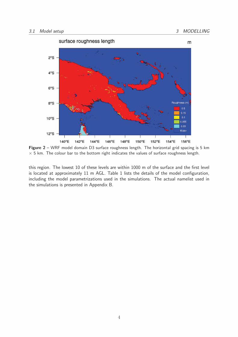
The simulations for the interim wind modelling were calculated on a grid with horizontalspacing of 45 km × 45 km (outer domain, D1, with 96 × 96 grid points), 15 km × 15 km(first nested domain, D2, with 187 × 187 grid points) and 5 km × 5 km (second nest, D3,with 325 × 397 grid points). Maps of the model domains are displayed in Fig. 1. The surfaceroughness length for innermost domain, D3, is given in Fig. 2.

In the vertical the model was configured with 50 levels with model top at 20 hPa. This isa special model configuration adapted to the occurrence of more deep convective activity in

2

3.1 Model setup 3 MODELLING

Figure 1 – WRF model domains configuration and terrain elevation (m). Top left: 45 km × 45 kmdomain (D1), top right: 15 km x 15 km (D2) and bottom: 5 km × 5 km (D3). The inner linesshow the position of D2 and D3 in D1 and D2, respectively. The colour scale indicates the terrainheight.

3

3.1 Model setup 3 MODELLING

Figure 2 – WRF model domain D3 surface roughness length. The horizontal grid spacing is 5 km× 5 km. The colour bar to the bottom right indicates the values of surface roughness length.

this region. The lowest 10 of these levels are within 1000 m of the surface and the first levelis located at approximately 11 m AGL. Table 1 lists the details of the model configuration,including the model parametrizations used in the simulations. The actual namelist used inthe simulations is presented in Appendix B.

4

3.1 Model setup 3 MODELLING

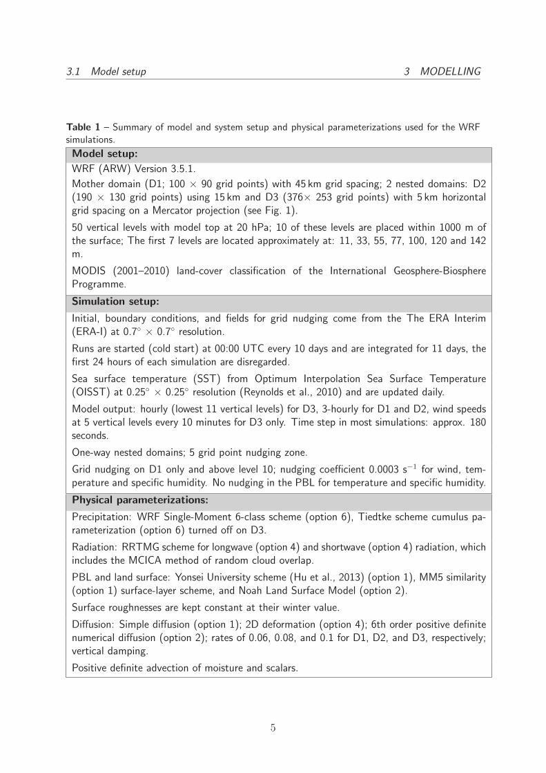
Table 1 – Summary of model and system setup and physical parameterizations used for the WRFsimulations.

Model setup:

WRF (ARW) Version 3.5.1.

Mother domain (D1; 100 × 90 grid points) with 45 km grid spacing; 2 nested domains: D2(190 × 130 grid points) using 15 km and D3 (376× 253 grid points) with 5 km horizontalgrid spacing on a Mercator projection (see Fig. 1).

50 vertical levels with model top at 20 hPa; 10 of these levels are placed within 1000 m ofthe surface; The first 7 levels are located approximately at: 11, 33, 55, 77, 100, 120 and 142m.

MODIS (2001–2010) land-cover classification of the International Geosphere-BiosphereProgramme.

Simulation setup:

Initial, boundary conditions, and fields for grid nudging come from the The ERA Interim(ERA-I) at 0.7◦ × 0.7◦ resolution.

Runs are started (cold start) at 00:00 UTC every 10 days and are integrated for 11 days, thefirst 24 hours of each simulation are disregarded.

Sea surface temperature (SST) from Optimum Interpolation Sea Surface Temperature(OISST) at 0.25◦ × 0.25◦ resolution (Reynolds et al., 2010) and are updated daily.

Model output: hourly (lowest 11 vertical levels) for D3, 3-hourly for D1 and D2, wind speedsat 5 vertical levels every 10 minutes for D3 only. Time step in most simulations: approx. 180seconds.

One-way nested domains; 5 grid point nudging zone.

Grid nudging on D1 only and above level 10; nudging coefficient 0.0003 s−1 for wind, tem-perature and specific humidity. No nudging in the PBL for temperature and specific humidity.

Physical parameterizations:

Precipitation: WRF Single-Moment 6-class scheme (option 6), Tiedtke scheme cumulus pa-rameterization (option 6) turned off on D3.

Radiation: RRTMG scheme for longwave (option 4) and shortwave (option 4) radiation, whichincludes the MCICA method of random cloud overlap.

PBL and land surface: Yonsei University scheme (Hu et al., 2013) (option 1), MM5 similarity(option 1) surface-layer scheme, and Noah Land Surface Model (option 2).

Surface roughnesses are kept constant at their winter value.

Diffusion: Simple diffusion (option 1); 2D deformation (option 4); 6th order positive definitenumerical diffusion (option 2); rates of 0.06, 0.08, and 0.1 for D1, D2, and D3, respectively;vertical damping.

Positive definite advection of moisture and scalars.

5

3.2 Data processing 3 MODELLING

Most choices in the model setup are fairly standard and used by other modelling groups.The only special setting for wind energy applications is the use of a constant surface roughnesslength, thus disabling the annual cycle available in the WRF model. This choice is consis-tent with the generalization procedure discussed in section 2 and Appendix A. A few otherparameterization settings are updated for equatorial conditions compared to other wind atlassimulations: more vertical levels and raised model top, more sophisticated microphysics andconvective scheme and updated radiation parameterizations.

Figure 3 – WRF model simulation schematic showing how the simulation period is covered by asuccession of overlapping 11 day simulations. The first day of the simulations, which overlaps withthe last day of the previous simulation, is for model spin-up and is not used in subsequent analysis.

The final simulation covered the 10-year period January 2004– December 2013, and wasrun in a series of 11-day long overlapping simulations, with the output from the first dayof each simulation being discarded, see Fig. 3. This method is based on the assumptionsdescribed in Hahmann et al. (2010) and Hahmann et al. (2014b). The simulation usedgrid nudging that continuously relaxes the model solution towards the gridded reanalysis butthis was done only on the outer domain and above the boundary layer (level 10 from thesurface) to allow for the mesoscale processes near the surface to develop freely. Because thesimulations were re-initialized every 10 days, the runs are independent of each other and canbe integrated in parallel reducing the total time needed to complete a multi-year climatology.The grid nudging and 10-days reinitialization keeps the model solution from drifting from theobserved large-scale atmospheric patterns, while the relatively long simulations guarantee thatthe mesoscale flow is fully in equilibrium with the mesoscale characteristic of the terrain.

3.2 Data processing

Wind speeds and directions are derived from the WRF model output, which represents 10-minutes or hourly instantaneous values. For evaluating the model wind speed climatology,the zonal and meridional wind components on their original staggered Arakawa-C grid wereinterpolated to the coordinates of the mass grid. The interpolated wind components were thenused to compute the wind speed. For a given height, e.g., 100 m, wind speeds are interpolated

6

4 RESULTS

between neighboring model levels using logarithmic interpolation in height. It was found thatthis interpolation procedure preserves more of the original features in the model wind profilecompared to other schemes (e.g., linear or polynomial interpolation of the wind components).The various data processing steps are shown in Fig. 4.

WRFData

reductionRaw 60min

Static

Raw 10min(Winds)

HeightInterpolation

10min(WindsT)

Data pro-cessing

Time-series Generalization .lib

Figure 4 – Schematic representation of the data processing used to create the wind climate filesthat compose the WRF-based NWA.

For each model grid point inside Papua New Guinea in domain D3 time-series for theentire period for the wind speed, wind direction at 5 heights, and 1/L were generated. Thegeneration of the time-series is a rather time consuming process because the WRF outputfiles are stored for every three hours for the whole domain. The generation of time-seriesrequires that for every grid-point in the considered region all files for the whole period haveto be accessed.

4 Results

In this section the results in the form of the annual mean wind climate are presented basedon the 10 years of simulation, covering the years 2004 to 2013 inclusive. First the simulatedwinds are presented. These represent the annual mean wind speed and power density at 100 ma.g.l. directly from the modelling, see Figs. 5 and 6. Therefore, the winds in these mapsreflect the orography and surface roughness length as they are represented in the model ratherthan the real orography and roughness length. Please note for the power density calculationonly the air density is constant at 1.25 kg/m3, so that variation of power density is due tovariation of the wind speed distribution alone. Before wind power production is calculated itis important to account for air density at the site of interest.

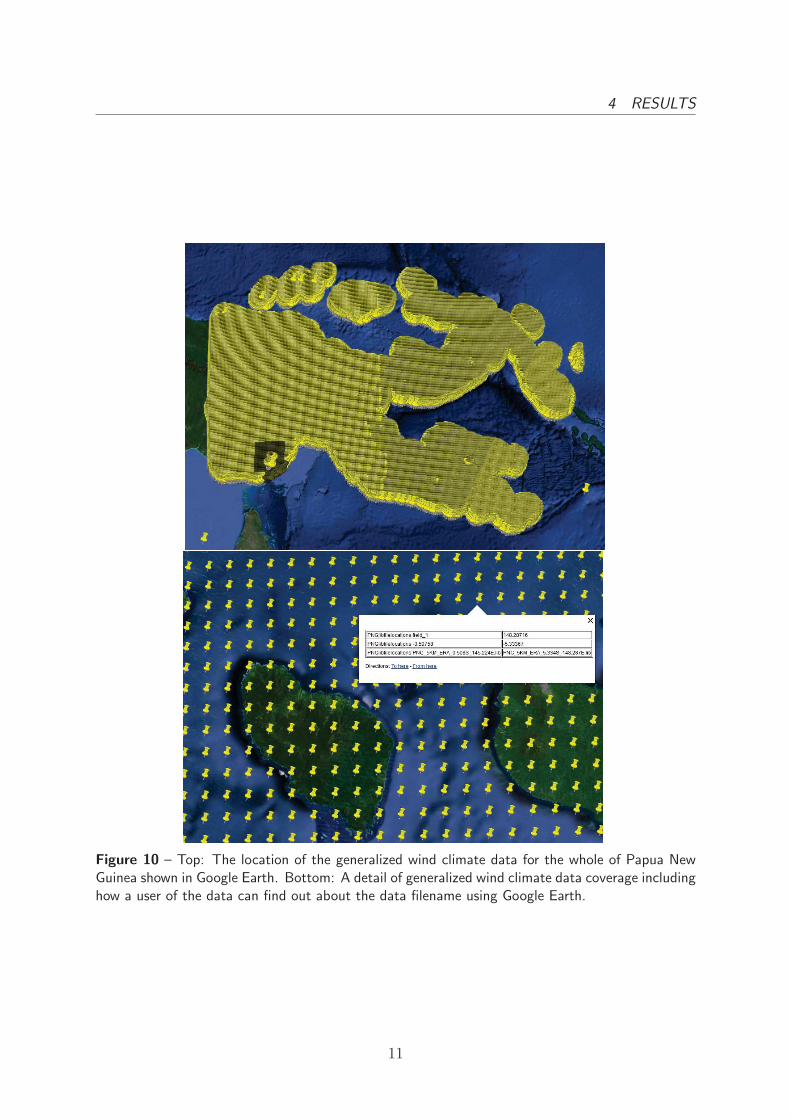
Next the generalized winds are presented. These represent the annual mean wind speed andpower density at 100 m a.g.l. for standardized condition of flat terrain with surface roughnesslength of 10 cm everywhere, as shown in Figs. 7 and 8. Now the winds in these maps reflectthe variation of the winds due to all influences other than the microscale orography and surfaceroughness change. The figures show only a small part of the information contained in thegeneralizated wind climate. An example of generalized wind climate file data is given in Fig.9. Figure 10 shows the location of the 43587 generalized wind climate files that are createdfor every WRF model grid point inside Papua New Guinea and surrounding waters. Thesefiles can be used in the WAsP software to calculate the predicted wind climate accounting forhighly detailed microscale orography and surface roughness change effects for a particular siteof interest.

7

4 RESULTS

Figure 5 – Mean annual simulated wind speed at 100 m a.g.l. from WRF simulation at 5 km × 5km grid spacing for the period 2004 to 2013 inclusive. The colour scale indicates the wind speed inm s−1.

Figure 6 – Mean annual simulated wind power density at 100 m a.g.l. from WRF simulation at 5km × 5 km grid spacing for the period 2004 to 2013 inclusive. The colour scale indicates the windpower density in Wm−2. Note: for the power density calculaton only the air density is constant at1.25 kg/m3.

8

4 RESULTS

Figure 7 – Mean annual generalized wind speed at 100 m a.g.l. from WRF simulation at 5 km × 5km grid spacing for the period 2004 to 2013 inclusive. The standard conditions are flat terrain withuniform surface roughness length (10 cm). The colour scale indicates the wind speed in m s−1.

Figure 8 – Mean annual generalized wind power density at 100 m a.g.l. from WRF simulation at5 km × 5 km grid spacing for the period 2004 to 2013 inclusive. The standard conditions are flatterrain with uniform surface roughness length (10 cm). The colour scale indicates the wind powerdensity in Wm−2. Note: for the power density calculation only the air density is constant at 1.25kg/m3.

9

4 RESULTS

Figure 9 – Example of the data contained within a generalized wind climate file data. This datacan be used in the WAsP software to make predictions of the wind resources at a specific site ofinterest accounting for the microscale effects due to orography and surface roughness changes. Thelocation is close to Launakalana.

10

4 RESULTS

Figure 10 – Top: The location of the generalized wind climate data for the whole of Papua NewGuinea shown in Google Earth. Bottom: A detail of generalized wind climate data coverage includinghow a user of the data can find out about the data filename using Google Earth.

11

6 CONCLUSIONS

5 Discussion and recommendations

An important issue to investigate further is whether the associated forest surface roughnesslength in the standard WRF modelling system needs to be changed. The standard roughnessfor a grid square composed of broadleaf evergreen trees is 0.5 m, which seems too low forsuch dense tropical forests. The generalization post-processing does take care of local errorsin surface roughness, but effects of a surface that is too smooth at the mesoscale might beimportant. Once measurements are available, a sensitivity study will be conducted varyingthe forest roughness through comparisons with local measured wind climates.

The measurement data is essential to the validation work required in Phase 3. Suggestionsfor regions for the measurement masts are given in Section C. The regions are choosen becausethey represent distinct locations with comparatively high wind speeds. The regions are meantsolely for guidance and only depict the regions from a wind climate perspective. Many otherfactors need to be considered (such as land ownership, ease of access, security etc) beforefinalizing measurement locations.

Through the measurements a better understanding of the wind energy relevant meteorol-ogy of the country will be gained, an improved configuration of the modelling system will bedeveloped and tested, and an uncertainty estimate of the final wind atlas can be determined.

6 Conclusions

This report has described the Phase 1 interim mesoscale wind modelling for Papua NewGuinea. The simulation methodology, the configuration of the WRF model and the general-ization method have been reported. The results of the wind modelling are presented in theform of simulated and generalized wind maps, and in the form of generalized wind climatedata files.

12

REFERENCES REFERENCES

References

Badger, J., H. Frank, A. N. Hahmann, and G. Giebel, 2014: Wind-climate estimation basedon mesoscale and microscale modeling: Statistical-dynamical downscaling for wind energyapplications. J. Appl. Meteor. Climatol., 53, 1901–1919.

Draxl, C., A. N. Hahmann, A. Pena, and G. Giebel, 2014: Evaluating winds and vertical windshear from WRF model forecasts using seven PBL schemes. Wind Energy, 17, 39–55.

Frank, H. and L. Landberg, 1997: Modelling the wind climate of Ireland. Bound.-Layer Me-

teor., 85 (3), 359–378, doi:{10.1023/A:1000552601288}.

Hahmann, A., C. Lennard, J. Badger, C. Vincent, M. Kelly, P. Volker, B. Argent, andJ. Refslund, 2014a: Mesoscale modeling for the Wind Atlas of South Africa (WASA)project. Tech. rep., http://orbit.dtu.dk/services/downloadRegister/102673293/Mesoscale_modeling.pdf, DTU Wind Energy.

Hahmann, A. N., D. Rostkier-Edelstein, T. T. Warner, F. Vandenberghe, Y. Liu, R. Babarsky,and S. P. Swerdlin, 2010: A Reanalysis System for the Generation of Mesoscale Climatogra-phies. J. Appl. Meteor. Clim., 49 (5), 954–972, doi:{10.1175/2009JAMC2351.1}.

Hahmann, A. N., C. L. Vincent, A. Pena, J. Lange, and C. B. Hasager, 2014b: Wind cli-mate estimation using WRF model output: method and model sensitivities over the sea.International Journal of Climatology, doi:10.1002/joc.4217.

Horvath, K., D. Koracin, R. Vellore, J. Jiang, and R. Belu, 2012: Sub-kilometer dynamicaldownscaling of near-surface winds in complex terrain using WRF and MM5 mesoscalemodels. J. Geophys. Res., 117, D11 111, doi:DOI10.1029/2012JD017432.

Hu, X.-M., P. M. Klein, and M. Xue, 2013: Evaluation of the updated ysu planetary boundarylayer scheme within wrf for wind resource and air quality assessments. jgr, Accepted.

Kelly, M. and I. Troen, 2014: Probabilistic stability and “tall” wind profiles: theory andmethod for use in wind resource assessment. Wind Energy, in press.

Larsen, X. G., J. Badger, A. N. Hahmann, and N. G. Mortensen, 2013: The selective dynamicaldownscaling method for extreme-wind atlases. Wind Energy, 16, 1167–1182, doi:10.1002/we.1544.

Larsen, X. G., S. Larsen, and A. N. Hahmann, 2012: Origin of the waves in A case-studyof mesoscale spectra of wind and temperature, observed and simulated’: Lee waves fromthe Norwegian mountains. Q. J. R. Meteorolog. Soc., 138 (662, Part A), 274–279, doi:{10.1002/qj.916}.

Pena, A. and A. N. Hahmann, 2012: Atmospheric stability and turbulence fluxes at Horns Rev— An intercomparison of sonic, bulk and WRF model data. Wind Energy, 15, 717–731,doi:DOI:10.1002/we.500.

Reynolds, R. W., C. L. Gentemann, and G. K. Corlett, 2010: Evaluation of aatsr and tmisatellite sst data. J. Climate, 23 (1), 152–165, doi:DOI10.1175/2009JCLI3252.1.

13

REFERENCES REFERENCES

Skamarock, W. C., et al., 2008: A Description of the Advanced Research WRF Version 3.Tech. Rep. NCAR/TN–475+STR, National Center for Atmospheric Research.

Storm, B., J. Dudhia, S. Basu, A. Swift, and I. Giammanco, 2009: Evaluation of the weatherresearch and forecasting model on forecasting low-level jets: implications for wind energy.Wind Energy, 12 (1), 81–90.

Troen, I. and E. L. Petersen, 1989: European Wind Atlas. Published for the Commission ofthe European Communities, Directorate-General for Science, Research, and Development,Brussels, Belgium by Risø National Laboratory.

Tuller, S. E. and A. C. Brett, 1984: The characteristics of wind velocity that favor the fittingof a Weibull distribution in wind-speed analysis. J. Appl. Meteor. Clim., 23 (1), 124–134,doi:10.1175/1520-0450(1984)0232.0.CO.

Vincent, C. L., A. N. Hahmann, and M. C. Kelly, 2012: Idealized mesoscale model simulationsof open cellular convection over the sea. Bound.-Layer Meteor., 142 (1), 103–121, doi:DOI10.1007/s10546-011-9664-7.

WASA, 2014: The Wind Atlas for South Africa. [Online], http://wasa.info.org.

14

A DETAILED DESCRIPTION OF GENERALIZATION

A Detailed description of generalization

A.1 Basic generalization equations

The generalization of WRF model winds is an extension of the KAMM/WAsP generalizationmethod described in Badger et al. (2014). In the first step, the time series of wind speedand direction are corrected for orography and roughness change, which are a function of winddirection and height. Given a time series of wind speed, u = u(z, t), and wind direction,φ = φ(z, t), which are functions of height and time, intermediate values, u and φ, are givenby

u =u

(1 + δAo)(1 + δAr)(1)

φ = φ− δφo, (2)

where δAo, δφo and δAr and are generalization factors for orography in wind speed anddirection and roughness change, respectively. From the time series of corrected wind speedand direction ”wind classes” are determined. The binning is based on wind direction sectors,wind speed and surface stability according to the Obukhov length as described in section A.2.From the binning, mean values of wind speed, u, and wind direction, φ and typical Obuhovlength L, together with the frequency of occurrence, F , of each bin are determined. Forsimplicity, we will drop the over-bar from the equations that follow, but it is understood thatthey are applied to the mean values of each bin and not the individual time series values.

From the corrected wind speed value we obtain an intermediary friction velocity, u∗

u∗ =κu

ln[(z/z0) + ψ(z/L)](3)

where z0 is the downstream surface roughness length and ψ is a stability correction functionthat adjust the logarithmic wind profile due to non-neutral stability conditions and κ is thevon Karman constant. The stability correction uses the relationship:

ψ(z/L) =

{

−31.58[1− exp(−0.19z/L)] if x ≥ 02 log[0.5(1 + x)] + log[0.5(1 + x2)]− 2 tan−1(x) + 1.5746 if x < 0

(4)

where x = (1 − 19z/L). We use this function with a typical value of the Obukhov lengthfrom each wind class bin (see table 2). This procedure avoids using the similarity theory onwind profiles that lie outside the bounds of validity of the theory and that sometimes occurin the WRF simulations.

In the next step, we use the geostrophic drag law, which is used for neutral conditions todetermine nominal geostrophic wind speeds, G, and wind directions, αG, are calculated, usingthe intermediate friction velocity and wind direction:

G =u∗κ

√

(

lnu∗f z0

− A

)2

+B2, (5)

sin φG = −sin−1(

B u∗

κG

)

, (6)

15

A.2 Sectorization A DETAILED DESCRIPTION OF GENERALIZATION

where A = 1.8 and B = 5.4 are two empirical parameters and f is the Coriolis parameter, andφG is the angle between the near-surface winds and the geostrophic wind. Near the equator,where f can become too large or undefined, it is reset to its value at a latitude of 10◦.

To obtain a new generalized friction velocity, u∗G, for a standard roughness length z0,std,Equation 5 is reversed by an iterative method,

G =u∗Gκ

√

(

lnu∗Gf z0,std

− A

)2

+B2, (7)

Finally, the generalized wind speed, uG, is obtained by using the logarithmic wind profile law

uG =u∗Gκ

ln

(

z

z0,std

)

. (8)

A.2 Sectorization

Table 2 – Stability ranges and typical values used in the generalization procedure.

Stability class Obukhov length Typical Obukhov value

range (m) L (m)Very unstable -50 < L < -100 -75Unstable -100 < L < -200 -150

Near unstable -200 < L < -500 -350Neutral L < -500; L > 500 10000

Near stable 200 < L < 500 350Stable 50 < L < 200 125

Very stable 10 < L < 50 30

To apply the generalization procedure to the WRF-model output, winds from the mesoscalemodel simulations are binned according to wind speed (usually in 2.5 m s−1 bins), winddirection (usually 48 sectors of 7.5◦ width) and seven stability class based on the Obukhovlength that is also an output from the WRF simulation. The ranges for the stability classesare listed in Table 2 together with the “typical” length used in the generalization.

The procedure is carried out for each model grid point independently. In practice, timeseries of wind speed and direction at the desired vertical levels and 1/L are extracted fromthe model output files. The generalization procedure is then carried out on each time seriesfile.

A.3 Weibull distribution fit

The frequency distribution of the horizontal wind speed can often be reasonably well describedby the Weibull distribution function (Tuller and Brett, 1984):

F (u) =kwAw

(

u

Aw

)kw−1

exp

[

−

(

u

Aw

)k]

, (9)

16

A.3 Weibull distribution fit A DETAILED DESCRIPTION OF GENERALIZATION

where F (u) is the frequency of occurrence of the wind speed u. In the Weibull distributionthe scale parameter Aw has wind speed units and is proportional to the average wind speedcalculated from the entire distribution. The shape parameter k(≥1) describes the skewnessof the distribution function. For typical wind speed distributions, the kw-parameter has valuesin the range of 2 to 3.

From the values of Aw and kw, the mean wind speed U (m s−1) and mean power densityE (Wm−2) in the wind can be calculated from:

U = AwΓ

(

1 +1

kw

)

(10)

E =1

2ρA3

w · Γ

(

1 +3

kw

)

(11)

where ρ is the mean density of the air and Γ is the gamma function. We use the moment fittingmethod as used in the Wind Atlas Analysis and Application Program (WAsP) for estimatingthe Weibull parameters. The method is described in detail in Troen and Petersen (1989).Basically this method estimates Aw and kw to fit the power density in the time series insteadof the mean wind speed.

The Weibull fit is done for the ensemble of wind speeds in each wind direction bin (usually12 direction sectors) for each standard height (usually 5 heights: 10, 25, 50, 100 and 200 m)and standard roughness lengths (usually 5 roughness: 0.0002 (water), 0.03, 0.1, 0.4, 1.5 m).The 25 Weibull fits for each wind direction sector use the method described above.

This sector-wise transformation of Weibull wind statistics—i.e. transforming the WeibullAw and kw parameters to a number of reference heights over flat land having given referenceroughnesses—uses not only the geostrophic drag law, but also a perturbation of the drag law,with the latter part including a climatological stability treatment. The transformation andstability calculation is consistent with that implemented in WAsP and outlined in Troen andPetersen (1989), with further details given in Kelly and Troen (2014). The transformationis accomplished via perturbation of both the mean wind and expected long-term variance ofwind speed, such that both Weibull-Aw and kw are affected. When purely neutral conditions(zero stability effects) are presumed for the wind statistics to be transformed, there is still aperturbation introduced, associated with the generalized (reference) conditions in the windatlas. This perturbation uses the default stability parameter values found in WAsP; it isnegated upon subsequent application of the generalized wind from a given reference heightand roughness to a site with identical height and surface roughness, using WAsP with itsdefault settings. The climatological stability treatment in the generalization depends on theunperturbed Weibull parameters and effective surface roughness (Troen and Petersen, 1989),as well as the mesoscale output heights and wind atlas reference heights (though the latterdisappears upon application of wind atlas data via WAsP).

Figure 11 shows the structure of the resulting WAsP ”lib” file. It is structured as WeibullAw’s and kw’s for each sector, height and standard roughness length. The first row containsinformation about the geographical location of the wind climate represented in the lib-file.The second row lists the number of roughness classes (5), heights (3), and sectors (12),respectively. In the third and fourth row, the actual roughness (m) and heights (m) are listed.Below these header lines, a succession of frequencies of wind direction (1 line), values ofWeibull-Aw (1 line) and Weibull-kw (1 line) for each roughness class and height are printed

17

B WRF NAMELIST

Figure 11 – Contents of WAsP generalized wind climate file. This climate is for a location close toLaunakalana.

for each sector (12 sectors per line). This type of file can be used and displayed (Figure 9) inWAsP.

B WRF namelist

&time_control

start_year = YY1, YY1, YY1

start_month = MM1, MM1, MM1

start_day = DD1, DD1, DD1

start_hour = HH1, HH1, HH1

start_minute = 00, 00, 00

start_second = 00, 00, 00

end_year = YY2, YY2, YY2

end_month = MM2, MM2, MM2

end_day = DD2, DD2, DD2

end_hour = HH2, HH2, HH2

end_minute = 00, 00, 00

end_second = 00, 00, 00

interval_seconds = 21600,

input_from_file = .T., .T., .T.

history_interval = 180,180, 60

frames_per_outfile = 1, 1, 3

restart = .false.,

restart_interval = 100000,

io_form_history = 2

18

B WRF NAMELIST

io_form_restart = 2

io_form_input = 2

io_form_boundary = 2

auxhist3_outname = "winds_d<domain>_<date>",

auxhist3_interval = 0, 0, 10

frames_per_auxhist3 = 1, 1, 6

io_form_auxhist3 = 2,

auxinput4_inname = "wrflowinp_d<domain>",

auxinput4_interval = 360,360,360

io_form_auxinput4 = 2,

debug_level = 0,

/

iofields_filename = "WAfields.txt","WAfields.txt","WAfields.txt"

ignore_iofields_warning = .false.,

&domains

time_step = 240,

time_step_fract_num = 0,

time_step_fract_den = 22,

max_dom = 3,

parent_id = 0, 1, 2

parent_grid_ratio = 1, 3, 3

s_we = 1, 1, 1

e_we = 100, 190, 376,

s_sn = 1, 1, 1

e_sn = 90, 130, 253,

s_vert = 1, 1, 1

e_vert = 50, 50, 50,

grid_id = 1, 2, 3

i_parent_start = 1, 20, 30,

j_parent_start = 1, 20, 25,

num_metgrid_levels = 33,

p_top_requested = 2000,

eta_levels = 1.0000, 0.9974, 0.9947, 0.9921, 0.9895,

0.9869, 0.9843, 0.9817, 0.9791, 0.9765,

0.9671, 0.9518, 0.9314, 0.9067, 0.8786,

0.8478, 0.8149, 0.7807, 0.7456, 0.7101,

0.6747, 0.6396, 0.6052, 0.5716, 0.5390,

0.5075, 0.4771, 0.4479, 0.4200, 0.3931,

0.3674, 0.3428, 0.3191, 0.2963, 0.2743,

0.2531, 0.2324, 0.2123, 0.1926, 0.1733,

0.1544, 0.1331, 0.1146, 0.0966, 0.0790,

0.0619, 0.0453, 0.0292, 0.0138, 0.000,

dx = 45000,15000, 5000,

19

B WRF NAMELIST

dy = 45000,15000, 5000,

parent_time_step_ratio = 1, 3, 3

feedback = 0,

smooth_option = 0,

/

&physics

mp_physics = 6, 6, 6,

ra_lw_physics = 4, 4, 4,

ra_sw_physics = 4, 4, 4,

radt = 10, 10, 10,

sf_sfclay_physics = 1, 1, 1,

sf_surface_physics = 2, 2, 2,

bl_pbl_physics = 1, 1, 1,

bldt = 0, 0, 0,

cu_physics = 6, 6, 0,

cudt = 0, 0, 0,

isftcflx = 2,

fractional_seaice = 1,

seaice_threshold = 0.,

isfflx = 1,

ifsnow = 0,

icloud = 1,

surface_input_source = 1,

num_land_cat = 20,

num_soil_layers = 4,

sst_update = 1,

maxiens = 1,

maxens = 3,

maxens2 = 3,

maxens3 = 16,

ensdim = 144,

/

&fdda

grid_fdda = 1, 0, 0

gfdda_inname = "wrffdda_d<domain>",

gfdda_end_h = 300, 0, 0

gfdda_interval_m = 360, 0, 0

fgdt = 0, 0, 0

if_no_pbl_nudging_uv = 0, 0, 0

if_no_pbl_nudging_t = 1, 0, 0

if_no_pbl_nudging_q = 1, 0, 0

if_zfac_uv = 1, 0, 0

k_zfac_uv = 10, 0, 0

if_zfac_t = 1, 0, 0

20

B WRF NAMELIST

k_zfac_t = 10, 0, 0

if_zfac_q = 1, 0, 0

k_zfac_q = 10, 0, 0

guv = 0.0003, 0.000075, 0.000075,

gt = 0.0003, 0.000075, 0.000075,

gq = 0.0003, 0.000075, 0.000075,

if_ramping = 0,

dtramp_min = 60.0,

io_form_gfdda = 2,

/

&dynamics

w_damping = 1,

diff_opt = 1,

km_opt = 4,

diff_6th_opt = 2, 2, 2

diff_6th_factor = 0.06, 0.08, 0.1

base_temp = 290.

damp_opt = 0,

zdamp = 5000., 5000., 5000.

dampcoef = 0.15, 0.15, 0.15

khdif = 0, 0, 0

kvdif = 0, 0, 0

non_hydrostatic = .true.,.true.,.true.

moist_adv_opt = 1, 1, 1

scalar_adv_opt = 1, 1, 1

/

&bdy_control

spec_bdy_width = 5,

spec_zone = 1,

relax_zone = 4,

specified = .true., .false.,.false.

nested = .false., .true., .true.

/

&grib2

/

&namelist_quilt

nio_tasks_per_group = 0,

nio_groups = 1,

/

21

C SUGGESTION FOR PHASE 2 MEASUREMENT REGIONS

C Suggestion for Phase 2 measurement regions

The regions indicated are areas in Papua New Guinea with relatively high wind resourcescompared to the rest of the domain. The regions can be used as guidance for decisions relatedto locating high verification masts.

Locations over the spine of the Papua New Guinea Highlands have higher modelled windsenhanced by their elevated exposure. Around Dura Island there are higher modelled winds inthe coastal areas. From Port Moresby and southward and eastward there are higher modelledwinds due to a combination of orographic blocking and stronger winds coming off the sea. Thecentral spine of New Britain and some coastal areas around the island have higher modelledwinds. In particular the western part of the island. Similiarly Umboi Island and surrounds havehigh winds due to the mesoscale channeling in the straits between New Britain and Morobe.Along the chain of islands from Bougainville Island, Latangai Island and Manus, some coastalareas and exposed ridges may have favourable conditions.

This meteorological guidance is intended to be combined with other considerations forwind measurement siting. The suggestion is not to have coverage of all parts of a selectedverification region, but to have one or two masts per regions, if possible. By doing so theconfidence level of the results will be lifted for the whole verification region. However it maybe that other siting constraints make this difficult or impossible.

22