wind-driven lateral circulation in a stratified estuary ... · wind-driven lateral circulation in...

Wind-driven lateral circulation in a stratified estuary and its effectson the along-channel flow

Yun Li1 and Ming Li1

Received 13 December 2011; revised 2 July 2012; accepted 17 July 2012; published 5 September 2012.

[1] In the stratified rotating estuary of Chesapeake Bay, the Ekman transport drivesa counterclockwise lateral circulation under down-estuary winds and a clockwise lateralcirculation under up-estuary winds (looking into estuary). The clockwise circulationis about twice as strong as the counterclockwise circulation. Analysis of the streamwisevorticity equation reveals a balance among three terms: titling of the planetary vorticityby vertical shear in the along-channel current, baroclinic forcing due to sloping isopycnalsat cross-channel sections, and turbulent diffusion. The baroclinic forcing is highlyasymmetric between the down- and up-estuary winds. While the counter-clockwise lateralcirculation tilts isopycnals vertically and creates lateral barolinic pressure gradient tooppose the Ekman transport under the down-estuary wind, the clockwise circulationinitially flattens the isopycnals and the baroclinic forcing reinforces the Ekman transportunder the up-estuary wind. The Coriolis acceleration associated with the lateral flowsis of the first-order importance in the along-channel momentum balance. It has a signopposite to the stress divergence in the surface layer and the pressure gradient in the bottomlayer, thereby reducing the shear in the along-channel current. Compared with thenon-rotating system, the shear reduction is about 30–40%. Two summary diagrams areconstructed to show how the averaged streamwise vorticity and along-channel currentshear vary with the Wedderburn (W ) and Kelvin (Ke) numbers.

Citation: Li, Y., and M. Li (2012), Wind-driven lateral circulation in a stratified estuary and its effects on the along-channelflow, J. Geophys. Res., 117, C09005, doi:10.1029/2011JC007829.

1. Introduction

[2] The wind-driven circulation in an estuary has previ-ously been interpreted in terms of the competition betweenthe wind stress and barotropic pressure gradient due to sealevel setup in the along channel direction [Weisberg andSturges, 1976; Wang, 1979; Garvine, 1985; Janzen andWong, 2002]. In a rectangular estuary or a stratified estu-ary where the buoyancy flux is strong, the along-channelflow consists of a vertically sheared two-layer circulation:downwind currents in the surface layer and upwind currentsin the bottom layer [e.g., Chen and Sanford, 2009; Reyes-Hernández and Valle-Levinson, 2010]. In estuaries withlateral variations of bathymetry, the depth-dependence in thelongitudinal momentum balance leads to laterally shearedthree-layer circulation: downwind currents on the shallowshoals and upwind flows in the center deep channel [e.g.,

Wong, 1994; Friedrichs and Hamrick, 1996]. However, thispicture of wind-driven circulation in a stratified rotatingestuary is incomplete.[3] Several studies have shown that along-channel winds

can drive strong lateral Ekman flows and isopycnal move-ments, generating upwelling/downwelling at shallow shoals[Malone et al., 1986; Sanford et al., 1990; Wilson et al.,2008; Scully, 2010]. These lateral motions are fundamentalto estuarine dynamics because they transport momentum[Lerczak and Geyer, 2004; Scully et al., 2009], alter stratifi-cation [Lacy et al., 2003; Li and Li, 2011] and transportsediment [Geyer et al., 2001; Chen et al., 2009]. For exam-ple, Li and Li [2011] showed that the wind-driven lateralcirculation causes lateral straining of the density field whichoffsets the effects of longitudinal straining. Furthermore,the lateral circulations provide an exchange pathway forbiologically important materials such as nutrients and oxy-gen, especially through lateral upwelling and downwelling[Malone et al., 1986; Sanford et al., 1990; Reynolds-Flemingand Luettich, 2004]. A recent study suggests that, in Chesa-peake Bay, the wind-driven lateral exchange of oxygenbetween shoal regions and deeper hypoxic areas is moreimportant than direct turbulent mixing through the pycnocline[Scully, 2010]. Despite these interesting studies, the dynamicsof wind-driven lateral circulations in stratified estuaries ofvarying width are still poorly understood. A simple scaling

1Horn Point Laboratory, University of Maryland Center forEnvironmental Science, Cambridge, Maryland, USA.

Corresponding author: Y. Li, Horn Point Laboratory, University ofMaryland Center for Environmental Science, 2020 Horn Point Rd.,Cambridge, MD 21613, USA. ([email protected])

This paper is not subject to U.S. copyright.Published in 2012 by the American Geophysical Union.

JOURNAL OF GEOPHYSICAL RESEARCH, VOL. 117, C09005, doi:10.1029/2011JC007829, 2012

C09005 1 of 17

suggests that the redistribution of momentum by lateral flowsis expected to play a larger role in narrow estuaries wherelateral gradients in the along-channel momentum are bigger.However, wider estuaries are expected to have a strongerlateral response to the along-channel wind-forcing becauseof rotation.[4] There have been a series of interesting studies on the

dynamics of lateral circulations in tidally driven estuaries.Several mechanisms have been proposed, including differ-ential advection [Nunes and Simpson, 1985; Lerczak andGeyer, 2004], bottom Ekman layer [Scully et al., 2009], dif-fusive boundary layer on a slope [Chen et al., 2009], channelcurvature [Chant, 2002] and lateral salinity gradient resultingfrom the presence of stratification [Lerczak and Geyer, 2004;Scully et al., 2009; Cheng et al., 2009]. Using a numericalmodel of an idealized estuarine channel, Lerczak and Geyer[2004] demonstrated that the lateral flows are driven pri-marily by differential advection and cross-channel densitygradients, and exhibit strong flood-ebb and spring-neap var-iability. In a subsequent study of Hudson River estuary,Scully et al. [2009] showed that nonlinear tidal advectionby lateral Ekman transport generates one-cell lateral circu-lation over flood-ebb tidal cycle, as found in an analyticmodel of Huijts et al. [2009]. Most of these previous studiesfocused on the analysis of the along-channel and cross-channelmomentum balance. Since the leading-order momentum bal-ance in the cross-channel direction is the thermal-wind bal-ance, Scully et al. [2009] discussed the ageostrophic termand provided insightful discussions on the interactionsbetween the lateral Ekman flows and lateral baroclinic pres-sure gradient. In this paper we develop a new approach toinvestigate the dynamics of lateral circulations. We willinvestigate the streamwise (along-channel) vorticity whichprovides a scalar representation of the lateral circulation, andconduct diagnostic analysis of the streamwise vorticity equa-tion to identify the generation and dissipation mechanisms.[5] A major motivation for studying the lateral circulation

in estuaries is the need to understand its effects on the along-channel estuarine exchange flows. In tidally driven estuaries,recent modeling investigations have demonstrated that thelateral advection is of the first-order importance in the along-channel momentum balance [Lerczak and Geyer, 2004;Scully et al., 2009; Cheng et al., 2009]. Burchard et al.[2011] and Burchard and Schuttelaars [2012] decomposedthe estuarine residual circulation into contributions fromprocesses such as tidal straining circulation, gravitationalcirculation, advectively driven circulation, and horizontalmixing circulation. They found that the lateral advection canbe a major driving force for the estuarine circulation in someestuaries. This motives us to examine the effects of the lat-eral flows on the wind-driven flows in the along-channeldirection. It will be shown that the Coriolis accelerationassociated with the lateral circulation is of the first-orderimportance in the along-channel momentum balance. Unlikethe nonlinear advection term which augments the along-channel flows, however, the Coriolis acceleration reducesthe shear in the along-channel current.[6] Using Chesapeake Bay as an example of a partially

mixed/stratified estuary, Li and Li [2011] investigatedhow the wind-driven lateral circulation causes the lateralstraining of density field and how this lateral straining off-sets the effects of longitudinal straining to reduce the

stratification-reduction asymmetry between the down- andup-estuary winds. This is a companion paper where weexamine the vorticity dynamics of the wind-driven lateralcirculation and its effects on the along-channel flows. Theplan for this paper is as follows. In Section 2 we describethe model configuration and introduce the analysis approach.Section 3 is devoted to the analysis of the streamwise vor-ticity equation while Section 4 is devoted to the analysisof the along-channel momentum balance. In Section 5, wesummarize the model results in a non-dimensional parameterspace consisting of the Wedderburn (W) and Kelvin (Ke)numbers.

2. Model Configuration and Analysis Approach

[7] To study wind-driven lateral flows, we use a 3Dhydrodynamic model of Chesapeake Bay based on ROMS(Regional Ocean Modeling System) [Li et al., 2005, 2007;Zhong and Li, 2006; Zhong et al., 2008; Li and Zhong, 2009].The model domain covers 8 major tributaries and a part ofthe coastal ocean to allow free exchange across the bay mouth(Figure 1). The total number of grid points is 120 � 80. Themodel has 20 layers in the vertical direction. A quadratic stressis exerted at the bed, assuming that the bottom boundary layeris logarithmic over a roughness height of 0.5 mm. The verticaleddy viscosity and diffusivity are computed using the k-klturbulence closure scheme [Warner et al., 2005] with thebackground diffusivity and viscosity set at 10�5 m2 s�1. Thehorizontal eddy viscosity and diffusivity are set to 1 m2 s�1.The model is forced by tides at the offshore boundary, byfreshwater inflows at river heads, and by winds across thewater surface. The open-ocean boundary condition consists ofChapman’s condition for surface elevation, Flather’s conditionfor barotropic velocity, Orlanski-type radiation condition forbaroclinic velocity, and a combination of radiation conditionand nudging (with a relaxation time scale of 1 day) for scalars[Marchesiello et al., 2001].[8] In this paper we conduct process-oriented idealized

modeling studies. At the open-ocean boundary, the model isforced by M2 tides only and salinity is fixed at 30 psu. Thetotal river discharge into the Bay is kept at the long-termaverage of 1500 m3 s�1 and is distributed to eight majortributaries according to observations: Susquehanna (51%),Patapsco (3.67%), Patuxent (3.67%), Potomac (18%),Rappahannock (4%), York (2%), James (14%), and Choptank(3.67%) [cf., Guo and Valle-Levinson, 2008]. We first runthe model without wind-forcing for 5 years so that the cir-culation and stratification in the Bay reaches a steady state.We then force the model with the along-channel (southwardor northward) winds of varying amplitudes and directions.Cross-channel (eastward or westward) winds are not con-sidered here because of fetch limitation. The wind stress isspatially uniform and is given by

tW ¼ tp sin w t � 25ð Þ½ � 25 ≤ t ≤ 27:50 other times

;

�ð1Þ

where tw is the along-channel wind stress, t the time (days),

w ¼ 2p5 day

the frequency of the wind-forcing, and tp the

peak wind stress. Positive tW corresponds to up-estuary

LI AND LI: WIND-DRIVEN LATERAL CIRCULATION C09005C09005

2 of 17

(northward) winds whereas negative tW corresponds todown-estuary (southward) winds. The maximum windstress magnitude tp ranges from 0.005 to 0.25 Pa, with thecorresponding range of 2.35 to 12.27 m s�1 for the windspeed (Table 1).[9] Previous investigations of lateral circulations in estu-

aries have mainly focused on the analysis of the cross-channel momentum equation [e.g., Lerczak and Geyer,2004; Scully et al., 2009]

∂v∂t|{z}

acceleration

¼ �fu|fflffl{zfflffl}Coriolisacceleration

� 1

r∂P∂y|fflfflffl{zfflfflffl}

pressure gradient

� u∂v∂x

þ v∂v∂y

þ w∂v∂z

� �|fflfflfflfflfflfflfflfflfflfflfflfflfflfflfflfflfflfflffl{zfflfflfflfflfflfflfflfflfflfflfflfflfflfflfflfflfflfflffl}

nonlinear advection

þ ∂∂z

KV∂v∂z

� �|fflfflfflfflfflfflfflffl{zfflfflfflfflfflfflfflffl}stress divergence

; ð2Þ

where (u, v, w) are the velocity components in the along-channel (x-), cross-channel (y-) and vertical (z-) directions.Consistent with the previous definition of the Wedderburnnumber [Chen and Sanford, 2009; Li and Li, 2011], thepositive x axis is pointed northward, the positive y axis ispointed westward, and the positive z axis is pointed upward.The lateral pressure gradient consists of two terms: lateralsea level slope and lateral density gradient.[10] Here we adopt a new approach by analyzing the

equation of the streamwise (along-channel) vorticity definedas wx ¼ ∂w

∂y � ∂v∂z . If one looks into estuary in the northern

hemisphere, a clockwise/counterclockwise lateral circulationcorresponds to positive/negative wx. The strength of lateralcirculation is represented by the absolute value of wx. Theequation for wx is given by

dwx

dt¼ f

∂u∂z

þ wx∂u∂x

þ wy∂u∂y

þ wz∂u∂z

� �

þ ∂∂y

� 1

r∂P∂z

� �� ∂∂z

� 1

r∂P∂y

� ��

þ ∂∂x

∂∂y

KH∂w∂x

� �� ∂∂z

KH∂v∂x

� ��

þ ∂∂y

∂∂y

KH∂w∂y

� �� ∂∂z

KH∂v∂y

� ��

þ ∂∂z

∂∂y

KV∂w∂z

� �� ∂∂z

KV∂v∂z

� �� ;

ð3Þ

where (wy, wz) are the vorticity components in the cross-channel and vertical directions, r the density, P the pressure,and KH and KV are eddy viscosity in the vertical and hori-zontal directions [cf., Kundu and Cohen, 2004]. Equation (3)shows that the streamwise vorticity wx can be generated bytilting of the planetary vorticity f due to the vertical shear inthe along-channel current, by vortex stretching/tilting, bybaroclinicity in the cross-channel section (misalignment ofpressure and density surfaces), and is diffused by subgrid-scale turbulent flows.[11] Making the Boussinesq approximation for the hori-

zontal momentum equations and the hydrostatic assumptionfor the vertical momentum equation, and assuming that the

Figure 1. Bathymetry of Chesapeake Bay and its adjacent coastal shelf. Major tributaries are marked.Depths are in meters. The shaded areas in the insert are used for calculating volume-averaged quantitiesin this study. The solid lines represent the along-channel and cross-channel transects.


3 of 17

variation in the along-channel direction is weak (i.e., ∂/∂x =0), we obtain the following simplifications:

wx ¼ � ∂v∂z

; wy ¼ ∂u∂z

; wz ¼ � ∂u∂y

; ð4Þ

P ¼ pa þ gr0hþ g

Z0

z

r′ z′ð Þdz′; ð5Þ

∂∂y

� 1

r∂P∂z

� �¼ ∂g

∂y¼ 0; ð6Þ

� ∂∂z

� 1

r∂P∂y

� �≈� ∂

∂z�g

∂h∂y

þ g

r0

Zz

0

∂r′∂y

dz′

0@

1A

¼ � g

r0

∂r′∂y

≈ �gb∂S∂y

; ð7Þ

in which pa is the atmospheric pressure, g the gravitationalconstant, h the sea surface height, r′ the density perturba-tions, and b the saline contraction coefficient. The last stepin equation (7) is derived by using the linear equation ofstate and assuming uniform temperature in the estuary.Substituting equations (4)–(7) into equation (3) leads to

dwx

dt¼ f

∂u∂z|fflfflfflfflfflfflfflfflfflfflffl{zfflfflfflfflfflfflfflfflfflfflffl}

tilting ofplanetary vorticity

�gb∂S∂y|fflfflfflfflffl{zfflfflfflfflffl}

baroclinicity

þ ∂2

∂z2KVwxð Þ|fflfflfflfflfflfflffl{zfflfflfflfflfflfflffl}

vertical diffusion

þ ∂2

∂y2KHwxð Þ|fflfflfflfflfflfflffl{zfflfflfflfflfflfflffl}

horizontal diffusion

;

ð8Þ

in which the horizontal eddy viscosity KH is assumed to be aconstant. In equation (8), the titling of planetary vorticity byshear in the along-channel flow and the baroclinicity due tothe sloping isopycnals in the cross-channel sections are twoterms generating the streamwise vorticity whereas the verti-cal and horizontal diffusion act to reduce it. The vorticitygeneration due to the stretching and tilting of relative vor-ticity is zero since ∂/∂x = 0. Equation (8) can also be derivedby taking �∂/∂z of equation (2) and using the hydrostaticapproximation to calculate the pressure distribution. In theROMS model, the equations of motions are solved in atransformed coordinate system which has a generalizedtopography-following s coordinate in the vertical directionand orthogonal curvilinear coordinates in the horizontaldirections [Haidvogel et al., 2000]. To utilize ROMS diag-nostic outputs for the analysis of vorticity dynamics, wetransform equation (8) into an equation in the ROMS coor-dinate. Please see Appendix B for details.[12] Another goal of this paper is to examine how the

wind-driven lateral circulation affects the along-channelflow. The along-channel momentum equation is given by

∂u∂t

¼ � 1

r∂P∂x|fflfflffl{zfflfflffl}

pressure gradient

þ ∂∂z

KV∂u∂z

� �|fflfflfflfflfflfflfflffl{zfflfflfflfflfflfflfflffl}stress divergence

þ fv|fflffl{zfflffl}Coriolisacceleration

� u∂u∂x

þ v∂u∂y

þ w∂u∂z

� �|fflfflfflfflfflfflfflfflfflfflfflfflfflfflfflfflfflffl{zfflfflfflfflfflfflfflfflfflfflfflfflfflfflfflfflfflffl}

nonlinear advection

:ð9Þ

The first two terms on the right-hand side of equation (9) arethe pressure gradient and stress divergence. The response ofan idealized rectangular estuary to axial wind-forcing isshown to consist of a vertically sheared two-layer circulationand has been interpreted in terms of the competition betweenthe stress divergence and pressure gradient due to sea levelsetup [e.g., Wang, 1979; Garvine, 1985; Janzen and Wong,2002]. The stress divergence overcomes the pressure

Table 1. Idealized Wind Experimentsa

Wind Stress(Pa)

Wind Speed(m/s)

Ke = 0.00 Ke = 1.04 Ke = 2.14 Ke = 4.50 Ke = 5.45 Ke = 6.76

Number W Number W Number W Number W Number W Number W

No Wind0.00 0.00 1 0 18 0 35 0 52 0 69 0 86 0

Down-Estuary Wind�0.005 �2.35 2 �0.24 19 �0.25 36 �0.27 53 �0.26 70 �0.25 87 �0.26�0.01 �3.20 3 �0.49 20 �0.51 37 �0.54 54 �0.52 71 �0.51 88 �0.52�0.02 �4.34 4 �0.97 21 �1.00 38 �1.07 55 �1.06 72 �1.00 89 �1.02�0.03 �5.17 5 �1.46 22 �1.50 39 �1.59 56 �1.57 73 �1.49 90 �1.52�0.05 �6.41 6 �2.46 23 �2.49 40 �2.63 57 �2.64 74 �2.46 91 �2.52�0.07 �7.37 7 �3.44 24 �3.49 41 �3.67 58 �3.71 75 �3.45 92 �3.52�0.15 �10.03 8 �7.66 25 �7.57 42 �7.82 59 �8.02 76 �7.34 93 �7.36�0.25 �12.27 9 �13.43 26 �13.15 43 �13.25 60 �13.42 77 �12.23 94 �12.01

Up-Estuary Wind0.005 2.35 10 0.26 27 0.26 44 0.27 61 0.26 78 0.25 95 0.260.01 3.20 11 0.52 28 0.53 45 0.56 62 0.53 79 0.51 96 0.530.02 4.34 12 1.04 29 1.08 46 1.13 63 1.09 80 1.03 97 1.080.03 5.17 13 1.56 30 1.65 47 1.72 64 1.65 81 1.54 98 1.640.05 6.41 14 2.56 31 2.85 48 2.98 65 2.74 82 2.61 99 2.780.07 7.37 15 3.57 32 4.04 49 4.34 66 3.93 83 3.73 100 3.900.15 10.03 16 7.45 33 8.39 50 9.56 67 9.77 84 8.69 101 9.120.25 12.27 17 12.32 34 13.61 51 15.49 68 16.74 85 16.14 102 17.36

aThe wind is spatially uniform and a temporal half-sinusoidal function from day 25 to 27.5, with peak wind stress shown below. Kelvin number (Ke) iscalculated using Coriolis parameter f that is 0, 25, 50, 100, 125 and 150 percent of the value for Chesapeake Bay. W is Wedderburn number. Both numbersare defined in Section 5.


4 of 17

gradient to drive the downwind flow in the surface layerwhereas the pressure gradient overcomes the stress diver-gence to drive the upwind flow in the bottom layer. If thelateral flows are strong, however, the Coriolis accelerationand nonlinear advection can also play important roles in thealong-channel momentum balance. They will be investi-gated in this paper. Appendices A and B give details on thediagnostic analyses of the momentum and vorticity equa-tions using ROMS model outputs.

3. Vorticity Dynamics of Lateral Circulation

[13] In Chesapeake Bay where the baroclinic Rossbyradius (about 5 km) is smaller than or comparable to thewidth of the estuary (5–20 km), the along-channel winds candrive lateral Ekman flows and isopycnal movements, gen-erating upwelling/downwelling at shallow shoals [Maloneet al., 1986; Sanford et al., 1990; Scully, 2010]. In this

section, we investigate the dynamics of wind-driven lateralcirculation using the streamwise vorticity as the primarydiagnostic quantity. First we show distributions of salinity,along- and cross-channel velocities at a cross-channel sec-tion, and study how they evolve during a down-/up-estuarywind event. We then examine temporal evolution of thestreamwise vorticity and conduct diagnostic analysis of thevorticity equation to explore the generation mechanisms forthe lateral circulation.[14] Figure 2 shows the estuary’s response to the down-

estuary (southward) wind with the peak wind stress tp =�0.07 Pa. We apply a 34-h low-pass filter to remove tidaloscillations. The southward wind drives a westward Ekmanflow (positive v) in the upper layer (about 4 m deep), whichin turn drives an eastward return flow (negative v) in thelower layer. A counterclockwise circulation thus appears inthe cross-channel section, with the cross-channel speedreaching about 0.1 m s�1 (Figure 2a). This circulation cell is

Figure 2. Temporal evolution of (a, d, and g) the streamwise vorticity (color) and the lateral-verticalvelocity vectors, (b, e, and h) the along-channel velocity, and (c, f, and i) salinity at a cross-channel sectionunder the down-estuary wind with the peak wind stress of �0.07 Pa. The snapshots are taken at 12-h intothe wind event (day 25.5), peak wind (day 26.25), and 12-h toward the end of wind (day 27). The plot islooking into estuary and the positive vorticity indicates clockwise motion.


5 of 17

situated over the deep channel and eastern shoal, but flowson the western shoal are directed eastward where a stronglateral salinity gradient exists (Figure 2c). The southwardwind drives a seaward along-channel flow (negative u) in theupper layer and a landward flow (positive u) in the lowerlayer, reinforcing the two-layer gravitational circulation(Figure 2b). However, the bottom return flow breaks into thesurface over the center channel. The counterclockwise lat-eral circulation strains the salinity field and tilts the iso-pycnals (isohalines) toward the vertical direction, as shownin Figure 2c (see Li and Li [2011] for a more detaileddiscussion).[15] At the peak wind, the surface Ekman layer deepens

to over 5 m depth and the lateral circulation strengthenssuch that the maximum cross-channel velocity reaches about0.15 m s�1 (Figure 2d). The along-channel current also getsstronger: both the downwind current in the upper layer andupwind current in the lower layer reach a maximum of0.30 m s�1 (Figure 2e). Continued vertical tilting of iso-pycnals and vertical mixing almost erase stratification in theupper layer, as shown in Figure 2f. In weakly stratified water,the effects of the bottom bathymetry become important suchthat the along-channel flows are laterally sheared with theupwind flow in the center channel [Csanady, 1973; Wong,1994; Winant, 2004]. During the set-down phase of thewind event, the counterclockwise circulation is still strong onthe eastern half of the cross-section, but flows on the westernhalf are directed eastward due to the lateral density gradientsthere (Figures 2g and 2i). Therefore, the wind-driven lateralcirculation in a stratified estuary is not solely determined bythe wind-forcing but is also affected by the cross-channeldensity gradient and vertical stratification.[16] The streamwise vorticity wx provides a concise

description of the lateral circulation, as shown in Figures 2a,2d, and 2g. The counterclockwise lateral circulation is repre-sented by negative values of wx. Strong negative vorticityemerges over the eastern half of the cross-channel section,which corresponds well with the counterclockwise circulationthere. Near the bottom boundary on the shallow shoals andinside the deep channel, v slows down as the bottom isapproached such that wx is positive. As the wind speedincreases, the magnitude of wx becomes larger and the regionof negative wx occupies a larger area of the water column.When the wind speed decreases, wx becomes weaker and thelateral circulation spins down.[17] The sense of the lateral circulation is reversed under

the up-estuary (northward) wind-forcing since the wind-driven Ekman transport is now directed eastward (Figure 3).The one-cell clockwise circulation extends over the wholecross-channel section, strengthens as the wind speed increa-ses, and then weakens as the wind speed decreases. Thecross-channel velocity v reaches a maximum speed of0.2 m s�1. Compared with counterclockwise circulationgenerated by the down-estuary wind, the clockwise circula-tion generated by the up-estuary wind is much stronger. Thedistribution of the streamwise vorticity wx also shows theasymmetry clearly: the magnitude of wx generated by the up-estuary wind is 2–3 times as large as that generated by thedown-estuary wind. The maximum value of wx reaches�11 � 10�2 s�1 at the peak wind. In the absence of wind-forcing, the along-channel flow features a seaward flow in asurface layer hugging the western shore and a landward flow

sitting in deep channel. The up-estuary northward windgenerates landward flows in the upper layer and seawardflows in the lower layer. Initially, the gravitational circulationstill dominates, as shown in Figure 3b. At the peak wind,however, the wind-driven circulation reverses the gravita-tional circulation, with the upper layer moving up-estuaryand the lower layer moving down-estuary (Figure 3e). Thiscirculation persists and gradually weakens until the end ofwind event. It should be noted that the along-channel flowgenerated by the up-estuary wind is about 1/3 to 1/2 ofthe flow generated by the down-estuary wind (compareFigures 3b, 3e, and 3h with Figures 2b, 2e, and 2h). More-over, the vertical stratification under the up-estuary wind issignificantly stronger than that under the down-estuary wind.Upwelling flows lift isopycnals on the western side up fromthe depressed positions (Figures 3c and 3f). Compared withthe down-estuary wind case (Figures 2c and 2f), the iso-pycnals appear to be more horizontal, and significant strati-fication is retained in the top 5 m and strong Ekman flowis confined to a relatively shallow surface layer. The strati-fication lessens the effects of bottom bathymetry on the flowstructure. Hence, the along-channel flows appear to be morevertically sheared than laterally sheared. During the secondhalf of the wind event, the continued straining of salinity fieldby the clockwise circulation tilts isopycnals toward the ver-tical direction (Figure 3i).[18] The above analysis suggests that the Ekman transport

is the primary driving force for the lateral circulation butother factors such as the lateral density gradient and verticalstratification also play important roles in determining thestrength of the lateral circulation. To gain insights into thegeneration mechanisms, we conduct diagnostic analysis ofthe streamwise vorticity equation and select the peak windas the time slice for the analysis. The dominant terms inthe vorticity budget are the titling of planetary vorticity by theshear in the along-channel flows, vertical diffusion and thebaroclinicity due to sloping isopycnals in cross-channel sec-tions. The horizontal diffusion term is two orders of magni-tude smaller than the vertical diffusion term. The nonlinearadvection term is weak, and the time tendency ∂wx/∂t is alsosmall (Figures 4g and 4h). Not surprisingly, the sign of thestreamwise vorticity (or the sense of the lateral circulation) isset by the tilting of planetary vorticity by the along-channelcurrent (Figures 4a and 4b). The down-estuary wind gen-erates the southward (negative) along-channel current. Thevertical shear bends f down toward the bay mouth and gen-erates a negative streamwise vorticity. In contrast, theup-estuary wind generates the northward (positive) along-channel current which tilts f to generate positive wx. Theturbulent diffusion acts to spin down wx and smooth thespatial gradients in wx (Figures 4c and 4d). This competi-tion between the tilting and diffusion terms provides aninterpretation of the Ekman-driven lateral circulation inunstratified channel from the vorticity point of view. Instratified estuaries such as Chesapeake Bay, the barolinicityforcing is important and is a major cause for the asymmetry inwx between the down-estuary and up-estuary winds. Withoutthe wind-forcing, the brackish plume is pushed to the westernshore, leading to higher sea level there. On the other hand,isopycnals are tilted downward on the western shore. Sincethe total pressure is the sum of the barotropic and baroclinicpressure, the isobars and isopycnals at the cross-channel


6 of 17

section are misaligned. The down-estuary wind steepens theslopes of the sea surface and isopycnals, particularly over thewestern half of the cross-channel section. Since the verti-cally tilted isopycnals tend to slump toward the horizontalequilibrium position, the baroclinic forcing generates posi-tive wx (Figure 4e). In contrast, the up-estuary wind lifts upthe isopycnals from their initial depressed positions on thewestern shoal (Figure 3f) such that the baroclinic forcing isrelatively weaker (Figure 4f).[19] The dynamics of the wind-driven lateral circulation

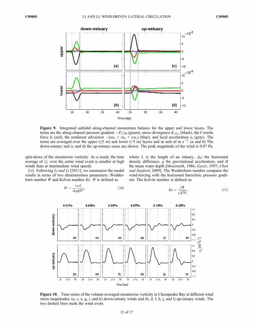
can be illustrated more clearly by averaging the streamwisevorticity over a control volume (see Figure 1) and calculatingthe volume-averaged terms in the vorticity equation (seeAppendix B). The volume-averaged wx has a small value of�0.069 � 10�2 s�1 before the onset of wind event(Figure 5a). It spins up as the wind stress increases and spinsdown as the wind decreases. A large difference is found in thestrength of wx between the down- and up-estuary winds. wx

peaks at�0.54� 10�2 s�1 during the down-estuary wind butat 1.32 � 10�2 s�1 (nearly 3 times larger) during the up-estuary wind (Figures 5a and 5c). To understand what causessuch an asymmetry, we compare the volume-averaged termsin the vorticity equation. Before the onset of wind-forcing,

the tilting of planetary vorticity f ∂u∂z (negative) is balanced by

the baroclinic forcing �gb ∂S∂y (positive), i.e., the along-

channel flow is in thermal wind balance with the lateraldensity gradient. This balance is disrupted by the wind-forcing, particularly during the up-estuary wind. The down-estuary wind amplifies the two-layer gravitational circulation

so that f ∂u∂z doubles (Figure 5b). In contrast, the up-estuary

wind generates a two-layer baroclinic current that opposesthe gravitational circulation. The shear in the along-channelcurrent is negative initially but turns to be positive as the up-estuary wind reverses the gravitational circulation (landward

Figure 3. Temporal evolution of (a, d, and g) the streamwise vorticity (color) and the lateral-verticalvelocity vectors, (b, e, and h) the along-channel velocity, and (c, f, and i) salinity at a cross-channel sectionunder the up-estuary wind with the peak wind stress of 0.07 Pa. The snapshots are taken at 12-h into thewind event (day 25.5), peak wind (day 26.25), and 12-h toward the end of wind (day 27). The plot is look-ing into estuary and the positive vorticity indicates clockwise motion.


7 of 17

in the upper layer and seaward in the lower layer). Conse-

quently f ∂u∂z is initially negative but becomes positive later

(Figure 5d). It should be noted that f ∂u∂z shows much larger

departure from its pre-wind value during the up-estuary windthan during the down-estuary wind. While the tilting of

planetary vorticity acts as a source for wx, the turbulent dif-fusion acts as a sink to spin down wx. The two terms arenearly 180� out of phase during the wind event. Due to thelateral straining of isopycnals, the eddy viscosity is 1.2 �10�3 m2 s�1, about 37% smaller than 1.9 � 10�3 m2 s�1

Figure 4. Terms in the streamwise-vorticity equation: (a and b) the tilting of planetary vorticity, (c and d)turbulent diffusion, (e and f) baroclinicity, and (g and h) time tendency under the down- and up-estuarywind with the peak magnitude of 0.07 Pa. The snapshots are taken at the peak of wind event. Thecross-section is looking into estuary, and positive values indicate clockwise rotation. The unit of vorticityterms is 10�6 s�2.

Figure 5. Time series of the volume-averaged (a and c) streamwise vorticity (wx) and (b and d) the termsin the vorticity equation: the tilting of planetary vorticity f (black solid), turbulent diffusion (black dashed),baroclinicity (red), nonlinear advection (blue) and time change rate (gray) under the down- and up-estuarywind with the peak magnitude of 0.07 Pa.


8 of 17

during down-estuary wind. However, the vertical gradient ofwx is much larger during the up-estuary wind. The net resultis that the turbulent diffusion of wx is much stronger duringthe up-estuary wind than during the down-estuary wind. Asshown in Figure 5, the time series of the volume-averageddiffusion appears to be a mirror image of the perturbation of

f ∂u∂z from its pre-wind value. This reveals a counter-balance

between the vorticity generation due to the titling of theplanetary vorticity and the vorticity destruction due to theturbulent diffusion. In comparison to the two terms, the non-linear advection term is small enough to be neglected(Figures 5b and 5d).[20] The baroclinic forcing is elevated during the down-

estuary wind since the counterclockwise circulation tilts theisopycnals toward the vertical direction and amplifies

�gb ∂S∂y . A more dramatic effect is noted during the up-

estuary wind when �gb ∂S∂y initially helps to generate the

clockwise lateral circulation but reduces to near zero valuesas the isopycnals slump back to horizontal equilibriumpositions. During the second half of the up-estuary windevent, continual upwelling on the western shoal lifts highsalinity bottom water to the surface and creates a negative

baroclinic forcing, but �gb ∂S∂y is relatively weak since the

isopycnals are widely spaced (see Figure 3i).[21] The feedback mechanisms between the baroclinicity

and lateral Ekman flows are different under the down- andup-estuary winds. When the estuary is forced by the down-estuary wind, the vertical shear in the along-channel currentresults in a negative vorticity (f ∂u

∂z < 0 ), but the counter-clockwise lateral circulation steepens the isopycnals, leadingto a positive vorticity (�gb ∂S

∂y > 0 ). A negative feedbackthus exists to weaken the lateral circulation. When theestuary is forced by the up-estuary wind, however, thealong-channel shear is reversed so that the positive stream-wise vorticity (f ∂u

∂z > 0) is produced. During the first half ofthe wind event, the baroclinic forcing �gb ∂S

∂y > 0 con-tributes to the generation of the positive streamwise vorticitybut weakens as the isopycnals are flattened. Further strainingof the density field by the clockwise circulation leads to aweak baroclinic forcing �gb ∂S

∂y < 0 that opposes f ∂u∂z > 0.

When integrated over the whole wind event, the baroclinicforcing is positive under both the down- and up-estuarywinds, and contributes to the generation of positive stream-wise vorticity and clockwise lateral circulation.

4. Effects on the Along-Channel Flow

[22] In tidally driven estuaries, recent studies have shownthat nonlinear advection by lateral flows is of the first order ofimportance in the subtidal along-channel momentum balanceand acts as a driving force for the estuarine exchange flows[Lerczak and Geyer, 2004; Scully et al., 2009]. In this sectionwe investigate how the wind-driven lateral circulation affectsthe along-channel flow.[23] Figure 6 shows a comparison of the along-channel and

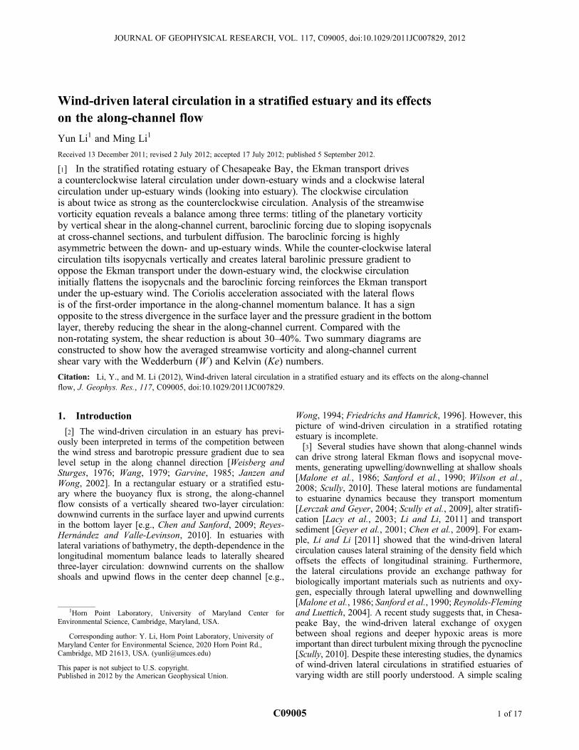
cross-channel velocities among three runs: (1) down-estuarywind; (2) no-wind; (3) up-estuary wind. Without wind-forcing, the estuary is characterized by a two-layer residualgravitational circulation with speeds reaching 0.1 m s�1,

as shown in the along-channel distribution of the along-channel velocity (Figure 6b). The lateral flows are weak andgenerated by the interaction between moderate tidal currentsand density field (Figure 6e). When the down-estuary windis applied over the Bay, it drives a seaward-directed currentin the upper layer and a return flow in the lower layer, thusamplifying the gravitational circulation in the along-channelsection (Figure 6a). A counterclockwise lateral circulationdevelops in the cross-channel section (Figure 6d). When thewind blows up-estuary, it drives a two-layer circulation thatopposes the gravitational circulation (Figure 6c). At the peakwind, the wind-driven circulation nearly cancels the gravita-tional circulation so that the along-channel flows are weak. Inthe meantime, a strong clockwise lateral circulation developsin the cross-channel section, with speeds comparable to thealong-channel currents (Figure 6f).[24] To determine if the lateral circulation affects the

along-channel flow, we conduct a diagnostic analysis of thealong-channel momentum equation (equation (9)), as shownin Figure 7. Both the down-estuary and up-estuary cases areconsidered and the time slice is selected at 12 h into the windevent. The stress divergence ∂

∂z KV∂u∂z

� and longitudinal

pressure gradient � 1r∂P∂x are two leading terms in the

momentum equation. It is interesting to note that the Coriolisforce fv exhibits a two-layer structure over the cross-channelsection. Under the down-estuary wind, the stress divergenceovercomes the pressure gradient to drive a downwind flow inthe upper layer. In the lower layer, the pressure gradientoverpowers the stress divergence to drive an upwind flow(Figures 7a and 7c). The Coriolis acceleration fv has theopposite sign to the stress divergence in the upper layer andthe opposite sign to the pressure gradient in the lower layer(Figure 7e). Hence it weakens the downwind current in theupper layer and the upwind current in the lower layer, therebyreducing the shear in the along-channel current. The sameresult applies to the up-estuary wind (Figures 7b, 7d, and 7f).Figure 8 is a schematic diagram that illustrates how theCoriolis acceleration on the lateral flows weakens the shear inthe along-channel currents under both down- and up-estuarywinds.[25] The nonlinear advection term � u ∂u

∂x þ v ∂u∂y þ w ∂u

∂z

�shows complex spatial patterns due to flow-topographyinteractions but is generally smaller than the Coriolis term(Figures 7g and 7h). It has no obvious correlation with otherterms in the momentum equation. Although the nonlinearadvection by tidally driven lateral circulation has been foundto play a significant role in driving the along-channel estu-arine exchange flows, we find that the nonlinear advectionby wind-driven lateral circulation does not play a coherentrole in driving the along-channel flows.[26] The above analysis is limited to a mid-bay cross-

section at one time snapshot. In order to compare the magni-tudes of each term in the along-channel momentum equationfor the whole Bay, we calculate the volume-averaged quanti-ties for the upper and lower layers. Since ∂

∂z KV∂u∂z

� switches

sign at a depth of around 5 m (see Figure 7), we define fixedvolumes for the upper and lower layers by separating them atthis depth. The time series of the layer-averaged terms areshown in Figure 9. We experiment with other ways for thevolume integration (e.g., chose a separation depth at 7 m) andobtain the same results.


9 of 17

[27] First we study the down-estuary wind. For the upperlayer, the stress divergence overcomes the along-channelpressure gradient to produce a negative value (with a maxi-mum of �3.59 � 10�6 m s�2) which drives the seawardflow. The Coriolis force acting the westward flows coun-teracts the stress divergence (with a maximum of 2.56 �10�6 m s�2) (Figure 9a). The nonlinear advection alsoslightly opposes the stress divergence term, but does notchange much with time. The local acceleration is relativelysmall and its sign change during the wind event is consistentwith the temporal development of the along-channel current.In the lower layer, the longitudinal pressure gradient over-powers the stress divergence to generate positive value (witha maximum of 2.36� 10�6 m s�2) and landward return flowwhereas fv < 0 (with a maximum of �1.66 � 10�6 m s�2).Once again the Coriolis term associated with the lateral flowopposes the pressure gradient that drives landward flow inthe lower layer (Figure 9b).[28] Under the up-estuary wind, the imbalance between

� 1r∂P∂x and

∂∂z KV

∂u∂z

� is much larger, reaching a maximum of

4.20 � 10�6 m s�2 in the upper layer and a minimum of

�4.39 � 10�6 m s�2 in the lower layer. Since the lateralcirculation is 2–3 times stronger under the up-estuary wind,fv is much larger, reaching a minimum of �3.84 � 10�6 ms�2 in the surface layer and a maximum of 3.13 � 10�6 ms�2 in the bottom layer. The nonlinear advection term playsa smaller role in the along-channel momentum balanceunder the up-estuary wind, as shown in Figures 7g and 7h.

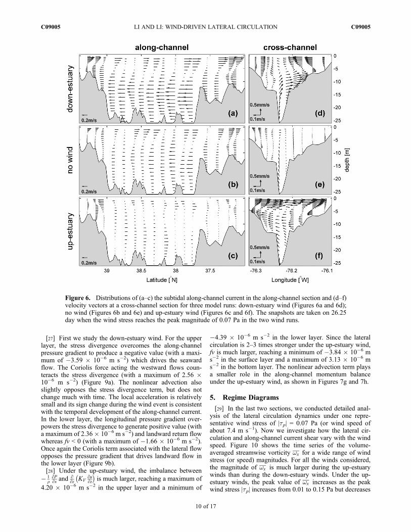
5. Regime Diagrams

[29] In the last two sections, we conducted detailed anal-ysis of the lateral circulation dynamics under one repre-sentative wind stress of |tp| = 0.07 Pa (or wind speed ofabout 7.4 m s�1). Now we investigate how the lateral cir-culation and along-channel current shear vary with the windspeed. Figure 10 shows the time series of the volume-averaged streamwise vorticity wx for a wide range of windstress (or speed) magnitudes. For all the winds considered,the magnitude of wx is much larger during the up-estuarywinds than during the down-estuary winds. Under the up-estuary winds, the peak value of wx increases as the peakwind stress |tp| increases from 0.01 to 0.15 Pa but decreases

Figure 6. Distributions of (a–c) the subtidal along-channel current in the along-channel section and (d–f)velocity vectors at a cross-channel section for three model runs: down-estuary wind (Figures 6a and 6d);no wind (Figures 6b and 6e) and up-estuary wind (Figures 6c and 6f). The snapshots are taken on 26.25day when the wind stress reaches the peak magnitude of 0.07 Pa in the two wind runs.


10 of 17

slightly as |tp| increases further to 0.25 Pa. In contrast, thepeak value of wx only exhibits modest increases as |tp|increases from 0.01 to 0.25 Pa. It is worth noting that athigh winds wx peaks earlier and decreases more rapidly with

time. An analysis of the streamwise vorticity budget (as inFigure 5) shows that both f ∂u

∂z and diffusion terms reachtheir maxima before the peak wind speed and suggests thatstrong turbulent dissipation at high winds causes a rapid

Figure 7. Distributions of the dominant terms in the subtidal along-channel momentum equation at across-channel section: (a and b) pressure gradient, (c and d) stress divergence, (e and f) Coriolis acceler-ation, (g and h) nonlinear advection, and (i and j) local acceleration. Figures 7a, 7c, 7e, 7g, and 7i are forthe down-estuary run and Figures 7b, 7d, 7f, 7h, and 7j are for the up-estuary run. The snapshots are takenat 12 h into the wind event with the peak magnitude of 0.07 Pa.

Figure 8. Conceptual diagram to illustrate the effects of Coriolis acceleration (fv, in blue) on the along-channel currents (u, in black). The lateral circulation is marked by red lines. The down-estuary wind gen-erates seaward flow in the upper layer and landward flow in the lower layer, but the Coriolis force on thecounterclockwise lateral circulation weakens this two-layer flow. The up-estuary wind generates landwardflow in the upper layer and seaward flow in the lower layer, but the Coriolis force on the clockwise lateralcirculation opposes this reversed two-layer flow.


11 of 17

spin-down of the streamwise vorticity. As a result, the timeaverage of wx over the entire wind event is smaller at highwinds than at intermediate wind speeds.[30] Following Li and Li [2011], we summarize the model

results in terms of two dimensionless parameters: Wedder-burn number W and Kelvin number Ke. W is defined as

W ¼ tWL

DrgH2; ð10Þ

where L is the length of an estuary, Dr the horizontaldensity difference, g the gravitational acceleration, and Hthe mean water depth [Monismith, 1986; Geyer, 1997; Chenand Sanford, 2009]. The Wedderburn number compares thewind-forcing with the horizontal baroclinic pressure gradi-ent. The Kelvin number is defined as

Ke ¼ fBffiffiffiffiffiffiffiffig′hS

p ; ð11Þ

Figure 9. Integrated subtidal along-channel momentum balance for the upper and lower layers. Theterms are the along-channel pressure gradient �Px/r0 (green), stress divergence Kvvzz (black), the Coriolisforce fv (red), the nonlinear advection �(uux + vuy + wuz) (blue), and local acceleration ut (gray). Theterms are averaged over the upper (≤5 m) and lower (>5 m) layers and in unit of m s�2. (a and b) Thedown-estuary and (c and d) the up-estuary cases are shown. The peak magnitude of the wind is 0.07 Pa.

Figure 10. Time series of the volume-averaged streamwise vorticity in Chesapeake Bay at different windstress magnitudes: (a, c, e, g, i, and k) down-estuary winds and (b, d, f, h, j, and l) up-estuary winds. Thetwo dashed lines mark the wind event.


12 of 17

where f is the Coriolis parameter, B the estuary width, g′ thereduced gravitational acceleration determined by the den-sity difference between the upper and lower layers, and hSthe mean depth of the upper layer. The Kelvin number isthe ratio of the estuary width to the internal Rossby radiusof deformation [e.g., Garvine, 1995; Valle-Levinson, 2008].For Chesapeake Bay, W varies from �1 to 10 for windspeeds ranging 5 � 10 m s�1 and Ke = 4.5. Although themodel bathymetry is specific to Chesapeake Bay, we

conduct numerical experiments by varying f over a rangefrom 25%f to 150%f to explore estuaries of differentwidths. Table 1 summarizes all the numerical runs we haveconducted.[31] Figure 11 shows how the time average of the

streamwise vorticity �wxh i over the entire wind event varieswith the Wedderburn and Kelvin numbers. �wxh i > 0(clockwise circulation) is for the up-estuary winds and�wxh i < 0 (counter-clockwise circulation) is for the down-estuary winds. At a given value of Ke, �wxh i increases rapidlywith increasing |W| at small values of |W|: the lateral circu-lation becomes stronger as the wind-forcing gets stronger.�wxh i reaches a maximum value at an intermediate value of|W |. At larger |W|, �wxh i decreases since the strong dissi-pation at high wind speeds causes a more rapid spin-downof the streamwise vorticity. As the lateral circulation isprimarily driven by the wind-induced Ekman transport, itis not surprising that �wxh i increases with increasing Ke: thelateral circulation is stronger at higher latitudes or in widerestuaries. It is important to note the asymmetry in �wxh ibetween the down- and up-estuary winds. At Ke = 4.5(at the latitude of Chesapeake Bay), �wxh i generated by theup-estuary winds is 2 times as large as that generated bythe down-estuary winds.[32] To better understand the variation of �wxh i with W and

Ke, we conduct a diagnostic analysis of the streamwise vor-ticity budget for all the model runs and plot the three leadingterms in Figure 12.We average the terms over the entire windevent to show the integrated effects. The tilting of planetary

vorticity by the along-channel current f ∂u∂z

D Eincreases with

both |W| and Ke. As expected, the generation of the stream-wise vorticity is stronger in a strongly rotating system or athigher winds. The turbulent diffusion acts in direct opposi-

tion to f ∂u∂z

D Eand shows similar variation with |W| and Ke.

While the tilting term tends to generate the lateral torque, theturbulent diffusion term tends to spin it down. The time-averaged baroclinic forcing term is positive during both the

Figure 11. The volume-averaged streamwise vorticity �wxh ias a function of Wedderburn (W) and Kelvin (Ke) numbers.Positive �wxh i indicates the clockwise circulation. TheW-axisis plotted in logarithmic scale with log2(|W| + 1) to revealrapid changes of �wxh i at low |W| values.

Figure 12. The volume-averaged terms in the streamwise vorticity as a function of Wedderburn (W ) andKelvin (Ke) numbers for all runs. The quantities are averaged over the whole wind event and in unit of10�6 s�2. Positive values correspond to the generation of clockwise circulation. W > 0 corresponds tothe up-estuary winds whereas W < 0 corresponds to the down-estuary winds.


13 of 17

down-estuary and up-estuary wind events. However, it ismuch larger during the down-estuary winds. This difference

in the baroclinic forcing �gb ∂S∂y

D Eis the main cause for the

asymmetry in the strength of the lateral circulation betweenthe down- and up-estuary winds. It is interesting to note that

�gb ∂S∂y

D Eapproaches to constant (saturating) values at large

values of |W| for a given value of Ke. The lateral straining canonly tilt the isopycnals toward the vertical directions and thelateral salinity gradient cannot increase further at higher windspeeds.[33] In Figure 13 we examine how the time average of the

along-channel current ∂u∂z

D Eover the entire wind event varies

with W and Ke. Ke = 0 corresponds to the non-rotating runs.At W = 0 the along-channel shear is generated by the grav-itational circulation and is negative. The down-estuary windsamplify this shear. The up-estuary winds generate a two-layer baroclinic current which opposes the gravitational

circulation. At low wind speeds, ∂u∂z

D Eremains to be negative

but turns to be positive (as the wind-driven circulationreverses the gravitational circulation) when W exceeds athreshold value. Compared with the rotating runs at the samevalue ofW, the shear in the along-channel current is strongestin the non-rotating runs. As discussed in section 4, theCoriolis force acting on the lateral flows reduces the shearin the along-channel current. At Ke = 4.5 (the latitude of

Chesapeake Bay), ∂u∂z

D Eis about 30–40% smaller than that

in runs in which the effects of the earth’s rotation are notconsidered. The reduction in the along-channel shear is

higher at higher latitudes and wide estuaries (larger valuesof Ke) but lower at lower latitudes and narrow estuaries.

6. Conclusions

[34] Using a numerical model of Chesapeake Bay, wehave investigated the dynamics of wind-driven lateral andalong-channel currents in a stratified rotating estuary. TheEkman transport associated with the along-channel windsgenerates a counterclockwise lateral circulation under thedown-estuary winds and a clockwise lateral circulation underthe up-estuary winds. However, the strength of the lateralcirculation is about 2 times stronger during the up-estuarywinds than during the down-estuary winds. To understandwhat causes this asymmetry, we have developed a newapproach by conducting diagnostic analysis of the stream-wise vorticity equation. It reveals a primary balance amongthree leading terms: the titling of the planetary vorticity bythe shear in the along-channel current, the baroclinic forcingdue to sloping isopycnals at cross-channel sections, and tur-bulent diffusion. Although the turbulent diffusion alwaysacts to spin down the vorticity generated by the titling ofthe planetary vorticity, the baroclinic forcing is highlyasymmetric between the down- and up-estuary winds. Thecounterclockwise lateral circulation generated by the down-estuary winds tilts the isopycnals toward the vertical direc-tions and creates adverse lateral barolinic pressure gradient tohamper the lateral Ekman transport. In contrast, the clock-wise lateral circulation generated by the up-estuary windsinitially flattens the isopycnals and the baroclinic forcingreinforces the lateral Ekman transport.[35] The analysis based on the streamwise vorticity could

be extended to study lateral circulations in tidally forcedestuaries. In the streamwise vorticity equation, the two-celllateral circulation generated by differential advection can bedescribed by the baroclinic forcing term �gb ∂S

∂y due to thelateral density gradient while the one-cell lateral circulationgenerated by the tidal rectification of lateral Ekman flow canbe described by the titling of the planetary vorticity by theshear in the tidal current f ∂u

∂z. An outstanding question is howthe two mechanisms contribute to the generation of the lat-eral circulations in estuaries of different widths and underdifferent river discharge and tidal forcing conditions.[36] Previous studies of lateral circulations in narrow

estuaries have shown that the nonlinear advection

� u ∂u∂x þ v ∂u

∂y þ w ∂u∂z

�associated with the lateral flows works

in concert with the along-channel baroclinic pressure gradi-ent to amplify the estuarine exchange flows. In a wideestuary such as Chesapeake Bay, however, we have foundthat the Coriolis acceleration fv associated with the lateralflows reduces the shear in the along-channel currents.Compared with the non-rotating system, the shear reductionis about 30–40%. Future work is needed to examine therelative roles of the nonlinear advection and Coriolis accel-eration in both tidally and wind-driven flows and for estu-aries of different widths. In an effort to generalize the modelresults specific to Chesapeake Bay, we have conductedmodel runs by varying the Coriolis parameter f. Regimediagrams have been constructed to show how the averagedstreamwise vorticity and along-channel current shear varywith the Wedderburn (W) and Kelvin (Ke) numbers. In the

Figure 13. The volume-averaged along-channel shear∂u=∂z

D Eas a function of Wedderburn (W ) and Kelvin

(Ke) numbers. Negative ∂u=∂zD E

corresponds to the sea-

ward flow in the upper layer and the landward flow in thelower layer.


14 of 17

future we plan to conduct model runs of an idealized genericestuary and examine how the lateral circulation and along-channel exchange flow vary in the nondimensional param-eter space.[37] The results presented in this paper are based on the

outputs from a numerical model. Although this model hasbeen validated against the observational data, there are to ourknowledge no existing data with adequate temporal andspatial resolution to resolve the full three-dimensionalstructure of flow and density fields. Given the physical andecological importance of the lateral circulations, especiallyfor long estuary with wide channels, future observationalstudy of the wind effects on lateral circulations is warranted.

Appendix A: Decomposition of Vectors Into Along-and Cross-Channel Directions

[38] We choose the along-channel direction to be alignedwith the semi-major axis of the depth-averaged tidal currentellipse associated with the dominant tidal harmonicsM2. It ispositive when pointing into the estuary. The cross-channeldirection is defined to be at 90 degree to the along-channeldirection. At each model grid point, the along- and cross-channel components of the horizontal velocity vector arecalculated using the following formulae:

~u ¼ uR cos qþ vR sin q; ðA1Þ~v ¼ �uR sin qþ vR cos q; ðA2Þ

where ~u;~vð Þ are the velocity components in the along- andcross-channel directions ~x;~yð Þ, (uR,vR) are the velocity com-ponents in the (x, h) directions defined in the ROMS model,and q is the angle between the along-channel direction andthe x-direction.[39] To project the momentum equations into the along-

and cross-channel directions, we treat each term in themomentum equation as a vector with components in the(x, h) directions and then apply the same decompositionas (A1)–(A2). If (x, h) are curvilinear coordinates, terms inthe momentum equations involve coefficients related to thecoordinate transformation [Haidvogel et al., 2000], but theprojection into the along- and cross-channel directions can betreated in the same way.

Appendix B: Calculation of Streamwise Vorticity

[40] In the Cartesian coordinate, the cross-channelmomentum equation is given by

∂v∂t

¼ �fu� 1

r∂P∂y

� u∂v∂x

þ v∂v∂y

þ w∂v∂z

� �þ ∂∂z

KV∂v∂z

� �

þ ∂∂x

KH∂v∂x

� �þ ∂∂y

KH∂v∂y

� �; ðB1Þ

where (u, v, w) are the velocity components in the along-channel, cross-channel and vertical directions, f the Coriolisparameter, P the total pressure, and Kv and KH are the ver-tical and horizontal eddy viscosities. As shown in Section 2,taking �∂/∂z of equation (B1) yields the equation for thestreamwise vorticity.[41] In the ROMS model, the equations of motions are

solved in a transformed coordinate system which has a

generalized topography-following s coordinate in the verti-cal direction and orthogonal curvilinear (x, h) coordinates inthe horizontal directions [Haidvogel et al., 2000]. After thedecomposition into the along- and cross-channel directions~x;~yð Þ , the cross-channel momentum equation in the trans-formed coordinates can be written as

∂~v∂t

z}|{accel

¼ �f ~uz}|{cor

þ � 1

r∂P∂~y

� grr0

∂z∂~y

� �zfflfflfflfflfflfflfflfflfflfflfflfflfflffl}|fflfflfflfflfflfflfflfflfflfflfflfflfflffl{prsgrd

þ � ∂~u~v∂~x

� ∂~v~v∂~y

þ CT

� �zfflfflfflfflfflfflfflfflfflfflfflfflfflfflfflfflfflffl}|fflfflfflfflfflfflfflfflfflfflfflfflfflfflfflfflfflffl{hadv

þ � 1

HZ

∂HZ~vW∂s

� �zfflfflfflfflfflfflfflfflfflfflfflffl}|fflfflfflfflfflfflfflfflfflfflfflffl{vadv

þ 1

HZ

∂∂s

KV

HZ

∂~v∂s

� �|fflfflfflfflfflfflfflfflfflfflfflffl{zfflfflfflfflfflfflfflfflfflfflfflffl}

vvisc

þ ~Dv|{z}hvisc

; ðB2Þ

in which the curvilinear transformation term (CT) is given by

CT ¼ HZ~u~v

mn

∂∂~x

mn

HZ

� �þ HZ~v~v

mn

∂∂~y

mn

HZ

� �

þ m ~u sin qþ ~v cos qð Þ ~u cos q� ~v sin qð Þ ∂∂~x

1

m

� �

þ m ~u cos q� ~v sin qð Þ2 ∂∂~y

1

m

� �

� n ~u sin qþ ~v cos qð Þ ~u cos q� ~v sin qð Þ ∂∂~x

1

n

� �

þ n ~u sin qþ ~v cos qð Þ2 ∂∂~y

1

n

� �: ðB3Þ

Here ~u;~vð Þ are the velocity components in the along- andcross-channel directions, W is the velocity component in thes-direction, m and n are the scale factors that relate the dif-ferential distances in x-h grid to the actual (physical) arclengths, Hz = ∂z/∂s, and ~Dv represents the horizontal vis-cosity terms. All the terms in the two horizontal momentumequations are calculated in the diagnostics package providedby ROMS. They can be combined to yield the terms in thealong- and cross-channel momentum equations using thedecomposition method described in Appendix A.[42] To obtain the equation for the streamwise vorticity,

we take the vertical derivative of equation (B2) and makeuse of ∂

∂z ¼ 1HZ

∂∂s. In the transformed coordinate system, the

streamwise vorticity is given by

wx ¼ � 1

HZ

∂~v∂s

ðB4Þ

and the equation of the streamwise vorticity becomes

∂wx

∂t¼ f

HZ

∂~u∂s

zfflfflffl}|fflfflffl{tilting of planetary vorticity

þ 1

HZ

∂∂s

1

r∂P∂~y

þ grr0

∂z∂~y

� �zfflfflfflfflfflfflfflfflfflfflfflfflfflfflfflfflfflfflfflffl}|fflfflfflfflfflfflfflfflfflfflfflfflfflfflfflfflfflfflfflffl{baroclinicity

þ 1

HZ

∂∂s

∂~u~v∂~x

þ ∂~v~v∂~y

� CT þ 1

HZ

∂ HZ~vWð Þ∂s

� �zfflfflfflfflfflfflfflfflfflfflfflfflfflfflfflfflfflfflfflfflfflfflfflfflfflfflfflfflfflfflfflfflfflfflfflfflfflffl}|fflfflfflfflfflfflfflfflfflfflfflfflfflfflfflfflfflfflfflfflfflfflfflfflfflfflfflfflfflfflfflfflfflfflfflfflfflffl{nonlinear advection

� 1

H2Z

∂2

∂s2

KV

HZ

∂~v∂s

� �|fflfflfflfflfflfflfflfflfflfflfflfflfflfflfflffl{zfflfflfflfflfflfflfflfflfflfflfflfflfflfflfflffl}

vertical diffusion

� 1

HZ

∂~Dv

∂s|fflfflfflfflfflfflffl{zfflfflfflfflfflfflffl}horizontal diffusion

: ðB5Þ


15 of 17

The nonlinear advection term is zero if the variation inalong-channel direction is zero, as assumed in the derivationof equation (8). In all the model runs considered in thispaper, the nonlinear advection term and horizontal diffusionterms are much smaller than the other terms in the stream-wise vorticity equation.[43] In this paper we integrate equation (B5) over a control

volume to examine the overall balance in the streamwisevorticity equation. The volume integration is defined as

wx ¼ ∯AwxdepthdA

∯AdA; ðB6Þ

where wxdepth ¼

Z V

�hwxdzZ V

�hdz

and A is the surface area of the

selected region.

[44] Acknowledgments. We thank Bill Boicourt, Malcolm Scully andPeng Jia for helpful discussions. We are grateful to NSF (OCE-082543 andOCE-0961880) and NOAA (CHRP-NA07N054780191) for the financialsupport. This is UMCES contribution 4682 and CHRP contribution 168.

ReferencesBurchard, H., and H. M. Schuttelaars (2012), Analysis of tidal strainingas driver for estuarine circulation in well-mixed estuaries, J. Phys.Oceanogr., 42(2), 261–271, doi:10.1175/JPO-D-11-0110.1.

Burchard, H., R. D. Hetland, E. Schulz, and H. M. Schuttelaars (2011),Drivers of residual estuarine circulation in tidally energetic estuaries:Straight and irrotational channels with parabolic cross section, J. Phys.Oceanogr., 41(3), 548–570, doi:10.1175/2010JPO4453.1.

Chant, R. J. (2002), Secondary circulation in a region of flow curvature:Relationship with tidal forcing and river discharge, J. Geophys. Res.,107(C9), 3131, doi:10.1029/2001JC001082.

Chen, S.-N., and L. P. Sanford (2009), Axial wind effects on stratificationand longitudinal salt transport in an idealized, partially mixed estuary,J. Phys. Oceanogr., 39(8), 1905–1920, doi:10.1175/2009JPO4016.1.

Chen, S.-N., L. P. Sanford, and D. K. Ralston (2009), Lateral circulation andsediment transport driven by axial winds in an idealized, partially mixedestuary, J. Geophys. Res., 114, C12006, doi:10.1029/2008JC005014.

Cheng, P., R. E. Wilson, R. J. Chant, D. C. Fugate, and R. D. Flood (2009),Modeling influence of stratification on lateral circulation in a stratified estu-ary, J. Phys. Oceanogr., 39(9), 2324–2337, doi:10.1175/2009JPO4157.1.

Csanady, G. T. (1973), Wind-induced barotropic motions in long lakes,J. Phys. Oceanogr., 3(4), 429–438, doi:10.1175/1520-0485(1973)003<0429:WIBMIL>2.0.CO;2.

Friedrichs, C. T., and J. M. Hamrick (1996), Effects of channel geometry oncross sectional variations in along channel velocity in partially stratifiedestuaries, in Buoyancy Effects on Coastal and Estuarine Dynamics, CoastalEstuarine Stud. Ser., vol. 53, edited by D. G. Aubrey and C. T. Friedrichs,pp. 283–300, AGU, Washington, D. C., doi:10.1029/CE053p283.

Garvine, R. W. (1985), A simple-model of estuarine subtidal fluctuationsforced by local and remote wind stress, J. Geophys. Res., 90(C6),1945–1948, doi:10.1029/JC090iC06p11945.

Garvine, R. W. (1995), A dynamical system for classifying buoyant coastaldischarges, Cont. Shelf Res., 15(13), 1585–1596, doi:10.1016/0278-4343(94)00065-U.

Geyer, W. R. (1997), Influence of wind on dynamics and flushing of shal-low estuaries, Estuarine Coastal Shelf Sci., 44(6), 713–722, doi:10.1006/ecss.1996.0140.

Geyer, W. R., J. D. Woodruff, and P. Traykovski (2001), Sediment trans-port and trapping in the Hudson River estuary, Estuaries Coasts, 24(5),670–679, doi:10.2307/1352875.

Guo, X. Y., and A. Valle-Levinson (2008), Wind effects on the lateral struc-ture of density-driven circulation in Chesapeake Bay, Cont. Shelf Res.,28(17), 2450–2471, doi:10.1016/j.csr.2008.06.008.

Haidvogel, D. B., H. G. Arango, K. Hedstrom, A. Beckmann, P. Malanotte-Rizzoli, and A. F. Shchepetkin (2000), Model evaluation experiments inthe North Atlantic Basin: Simulations in nonlinear terrain-following coor-dinates, Dyn. Atmos. Oceans, 32(3), 239–281, doi:10.1016/S0377-0265(00)00049-X.

Huijts, K., H. Schuttelaars, H. De Swart, and C. Friedrichs (2009), Analyt-ical study of the transverse distribution of along-channel and transverseresidual flows in tidal estuaries, Cont. Shelf Res., 29(1), 89–100,doi:10.1016/j.csr.2007.09.007.

Janzen, C. D., and K. C. Wong (2002), Wind-forced dynamics at theestuary-shelf interface of a large coastal plain estuary, J. Geophys. Res.,107(C10), 3138, doi:10.1029/2001JC000959.

Kundu, P. K., and I. M. Cohen (2004), Fluid Mechanics, 3rd ed., 759 pp.,Elsevier Acad., San Diego, Calif.

Lacy, J. R., M. T. Stacey, J. R. Burau, and S. G. Monismith (2003), Interac-tion of lateral baroclinic forcing and turbulence in an estuary, J. Geophys.Res., 108(C3), 3089, doi:10.1029/2002JC001392.

Lerczak, J. A., and W. R. Geyer (2004), Modeling the lateral circulation instraight, stratified estuaries, J. Phys. Oceanogr., 34(6), 1410–1428.

Li, M., and L. J. Zhong (2009), Flood-ebb and spring-neap variations ofmixing, stratification and circulation in Chesapeake Bay, Cont. ShelfRes., 29(1), 4–14, doi:10.1016/j.csr.2007.06.012.

Li, M., L. Zhong, and W. C. Boicourt (2005), Simulations of ChesapeakeBay estuary: Sensitivity to turbulence mixing parameterizations and com-parison with observations, J. Geophys. Res., 110, C12004, doi:10.1029/2004JC002585.

Li, M., L. Zhong, W. C. Boicourt, S. L. Zhang, and D. L. Zhang (2007),Hurricane-induced destratification and restratification in a partially mixedestuary, J. Mar. Res., 65(2), 169–192.

Li, Y., and M. Li (2011), Effects of winds on stratification and circulation ina partially mixed estuary, J. Geophys. Res., 116, C12012, doi:10.1029/2010JC006893.

Malone, T. C., W. M. Kemp, H. W. Ducklow, W. R. Boynton, J. H. Tuttle,and R. B. Jonas (1986), Lateral variation in the production and fate of phy-toplankton in a partially stratified estuary,Mar. Ecol. Prog. Ser., 32(2–3),149–160, doi:10.3354/meps032149.

Marchesiello, P., J. McWilliams, and A. Shchepetkin (2001), Open bound-ary conditions for long-term integration of regional oceanic models,Ocean Modell., 3(1–2), 1–20, doi:10.1016/S1463-5003(00)00013-5.

Monismith, S. (1986), An experimental-study of the upwelling response ofstratified reservoirs to surface shear-stress, J. Fluid Mech., 171, 407–439,doi:10.1017/S0022112086001507.

Nunes, R., and J. Simpson (1985), Axial convergence in a well-mixed estu-ary, Estuarine Coastal Shelf Sci., 20(5), 637–649, doi:10.1016/0272-7714(85)90112-X.

Reyes-Hernández, C., and A. Valle-Levinson (2010), Wind modificationsto density-driven flows in semienclosed, rotating basins, J. Phys. Ocea-nogr., 40(7), 1473–1487, doi:10.1175/2010JPO4230.1.

Reynolds-Fleming, J. V., and R. A. Luettich (2004), Wind-driven lateralvariability in a partially mixed estuary, Estuarine Coastal Shelf Sci.,60(3), 395–407, doi:10.1016/j.ecss.2004.02.003.

Sanford, L. P., K. G. Sellner, and D. L. Breitburg (1990), Covariability ofdissolved-oxygen with physical processes in the summertime ChesapeakeBay, J. Mar. Res., 48(3), 567–590.

Scully, M. E. (2010), Wind modulation of dissolved oxygen in ChesapeakeBay, Estuaries Coasts, 33(5), 1164–1175, doi:10.1007/s12237-010-9319-9.

Scully, M. E., W. R. Geyer, and J. A. Lerczak (2009), The influence of lat-eral advection on the residual estuarine circulation: A numerical modelingstudy of the Hudson River estuary, J. Phys. Oceanogr., 39(1), 107–124,doi:10.1175/2008jpo3952.1.

Valle-Levinson, A. (2008), Density-driven exchange flow in terms of theKelvin and Ekman numbers, J. Geophys. Res., 113, C04001,doi:10.1029/2007JC004144.

Wang, D. P. (1979), Wind-driven circulation in the Chesapeake Bay, winter1975, J. Phys. Oceanogr., 9(3), 564–572, doi:10.1175/1520-0485(1979)009<0564:WDCITC>2.0.CO;2.

Warner, J. C., W. R. Geyer, and J. A. Lerczak (2005), Numerical modelingof an estuary: A comprehensive skill assessment, J. Geophys. Res., 110,C05001, doi:10.1029/2004JC002691.

Weisberg, R. H., and W. Sturges (1976), Velocity observations in the WestPassage of Narragansett Bay: A partially mixed estuary, J. Phys. Oceanogr.,6(3), 345–354, doi:10.1175/1520-0485(1976)006<0345:VOITWP>2.0.CO;2.

Wilson, R. E., R. L. Swanson, and H. A. Crowley (2008), Perspectives onlong-term variations in hypoxic conditions in western Long Island Sound,J. Geophys. Res., 113, C12011, doi:10.1029/2007JC004693.


16 of 17

Winant, C. (2004), Three-dimensional wind-driven flow in an elongated,rotating basin, J. Phys. Oceanogr., 34(2), 462–476, doi:10.1175/1520-0485(2004)034<0462:TWFIAE>2.0.CO;2.

Wong, K. C. (1994), On the nature of transverse variability in a coastal-plain estuary, J. Geophys. Res., 99(C7), 14,209–14,222, doi:10.1029/94JC00861.

Zhong, L., and M. Li (2006), Tidal energy fluxes and dissipation inthe Chesapeake Bay, Cont. Shelf Res., 26(6), 752–770, doi:10.1016/j.csr.2006.02.006.

Zhong, L., M. Li, and M. G. G. Foreman (2008), Resonance and sea levelvariability in Chesapeake Bay, Cont. Shelf Res., 28(18), 2565–2573,doi:10.1016/j.csr.2008.07.007.


17 of 17

wind-driven lateral circulation in a stratified estuary ... · wind-driven lateral circulation in...

Documents