DOT/FAA/TC-15/19 Federal Aviation Administration William J. Hughes Technical Center Aviation Research Division Atlantic City International Airport New Jersey 08405

Aeroelastic Variability and Uncertainty of Composite Aircraft

September 2017 Final Report This document is available to the U.S. public through the National Technical Information Services (NTIS), Springfield, Virginia 22161. This document is also available from the Federal Aviation Administration William J. Hughes Technical Center at actlibrary.tc.faa.gov.

U.S. Department of Transportation Federal Aviation Administration

NOTICE

This document is disseminated under the sponsorship of the U.S. Department of Transportation in the interest of information exchange. The U.S. Government assumes no liability for the contents or use thereof. The U.S. Government does not endorse products or manufacturers. Trade or manufacturers’ names appear herein solely because they are considered essential to the objective of this report. The findings and conclusions in this report are those of the author(s) and do not necessarily represent the views of the funding agency. This document does not constitute FAA policy. Consult the FAA sponsoring organization listed on the Technical Documentation page as to its use. This report is available at the Federal Aviation Administration William J. Hughes Technical Center’s Full-Text Technical Reports page: actlibrary.tc.faa.gov in Adobe Acrobat portable document format (PDF).

Technical Report Documentation Page 1. Report No. DOT/FAA/TC-15/19

2. Government Accession No. 3. Recipient's Catalog No.

4. Title and Subtitle AEROELASTIC VARIABILITY AND UNCERTAINTY OF COMPOSITE AIRCRAFT

5. Report Date September 2017

6. Performing Organization Code

7. Author(s) Eli Livne, Andrey Styuart, Marat Mor, Luciano Demasi

8. Performing Organization Report No.

9. Performing Organization Name and Address William E. Boeing Department of Aeronautics & Astronautics University of Washington Box 352400 Seattle, WA 98195-2400

10. Work Unit No. (TRAIS)

11. Contract or Grant No.

12. Sponsoring Agency Name and Address U.S. Department of Transportation Federal Aviation Administration Office of Aviation Research Washington, DC 20591

13. Type of Report and Period Covered Final Report 2004-2010

14. Sponsoring Agency Code AIR-100

15. Supplementary Notes The FAA William J. Hughes Technical Center Aviation Research Division COR was Lynn Pham.

16. Abstract This report summarizes the work done at the University of Washington to contribute to the development of aeroelastic technology for the emerging fleet of composite airframe passenger and cargo aircraft. The objectives were to develop a probabilistic method to estimate aeroelastic reliabilities suitable for design, inspection, and regulatory compliance and to develop efficient, practical numerical simulation techniques for nonlinear composite airframes. Three test cases were studied: a two-dimensional (2D) airfoil/aileron, a 3-dimensional (3D) finite element-based low aspect ratio fighter-type wing/flaperon, and a composite vertical tail/rudder model. The first test case started with a simple 2D model and progressed to more complicated 3D models. The first two test cases were used to simulate linear flutter and gust response behavior as well as nonlinear behavior due to freeplay or other local nonlinearities. The third case focused on the flutter reliability of a passenger aircraft’s composite vertical tail/rudder system. The probabilistic methods used in this study effectively quantified the flutter reliability but were case-dependent. 17. Key Words Aeroelasticity, Aeroelastic, Composite airframes, Uncertainty, Reliability

18. Distribution Statement This document is available to the U.S. public through the National Technical Information Service (NTIS), Springfield, Virginia 22161. This document is also available from the Federal Aviation Administration William J. Hughes Technical Center at actlibrary.tc.faa.gov.

19. Security Classif. (of this report) Unclassified

20. Security Classif. (of this page) Unclassified

21. No. of Pages 63

22. Price

Form DOT F 1700.7 (8-72) Reproduction of completed page authorized

iii

ACKNOWLEDGEMENTS

This work was supported by a Federal Aviation Administration (FAA) research grant, “Combined Global/Local Variability and Uncertainty in Integrated Aeroservoelasticity of Composite Aircraft.” Peter Shyprykevich, Curtis Davies, and Lynn Pham were the technical monitors. Dr. Larry Ilcewicz was the technical advisor. The authors wish to thank the FAA Center of Excellence at the University of Washington’s Advanced Materials in Transport Aircraft Structures (AMTAS) for its support and sponsorship as well as Professor Mark Tuttle, head of the AMTAS. Thanks also to Dr. Luciano Demasi (who is now an associate professor at San Diego State University), Dr. Andrey Styuart, Dr. Marat Mor (now a private consultant and an affiliate associate professor of aeronautics and astronautics at the University of Washington), and Francesca Paltera (formerly a graduate student at the University of Washington’s mechanical engineering department) for their contributions to this work. Colleagues at The Boeing Company who supported this effort and contributed significantly to this work are Dr. James Gordon, Jeffrey Bland, Frank Roney, Carl Niedermeyer (now at the FAA), and Dr. Kumar Bhatia. This project has been wide in scope. It is only through such support and collaboration that it could lead to the tools, insights, and new results obtained and described in this report.

iv

TABLE OF CONTENTS

Page

EXECUTIVE SUMMARY xi

1. INTRODUCTION 1

2. THE PROBABILISTIC NONLINEAR 3 DOF AEROELASTIC SYSTEMWITHOUT AND WITH FREEPLAY 3

2.1 Background 3 2.2 Linear Flutter 6 2.3 A 2D 3 DOF system Limit Cycle Oscillation 8 2.4 Automated Finite Element-based flutter analysis for statistical aeroelastic

studies of uncertain airframes 11

3. PROBABILISTIC CONSIDERATIONS 15

3.1 General Approach 15 3.2 Statistics of extreme FLIGHT speeds of operation 16 3.3 Probabilistic characterization of airplane flutter speeds in a fleet 19 3.4 Systemic uncertainties 23 3.5 Flight testing 24 3.6 Contribution of other safety measures 27 3.7 The POF 27 3.8 Probability of flutter failure with changes of airframe dynamic properties over

time 30 3.9 Flutter probability formulation allowing for material degradation,

environmental effects, inspection procedures, damage, and repair 31

4. PROBABILISTIC 3D PROBLEMS 34

4.1 The Fighter Wing/Flap Configuration 34

4.1.1 Problem Definition 34 4.1.2 Results for the Fighter Type Wing 38

4.2 The Uncertain Aeroelastic Composite Vertical Tail/Rudder System 39

4.2.1 The Model 39 4.2.2 Results for the Composite Vertical Tail/Rudder System 42 4.2.3 Flutter Reliability of Damaged and Undamaged Composite Airframes 46

5. CONCLUSIONS 47

6. REFERENCES 48

v

LIST OF FIGURES

Figure Page

1 The 2D 3 DOF airfoil/aileron system 4

2 Empirical CDF of flutter speed Vf (m/sec) of the 2D 3 DOF airfoil/control surface system 7

3 Probabilistic sensitivity factors for 3DOF 2D airfoil/control surface system 8

4 Control surface hinge freeplay 9

5 Normalized LCO amplitudes (rad) of the nominal airfoil/aileron system 9

6 Distribution of LCO aileron rotation amplitudes (rad) in a sample of time response simulation 10

7 Scatter of LCO RMS amplitude response for the 3 DOF 2D aeroelastic system with hinge freeplay 11

8 Flow chart diagram of an automated system for reliability and damage assessment involving flutter 12

9 Flight speed exceedance curve approximations 17

10 CDF of maximum flight speed per 50,000 flight hours in flaps-retracted configuration 18

11 CDF of maximum flight speed per 50,000 flight hours in flaps-extended configuration 19

12 Empirical CDF for the accuracy of analytical flutter prediction 24

13 CDF of flutter speed before and after flight tests with an unconservative design and no damage assumed 25

14 CDF of flutter speed before and after flight tests (systemic analysis errors accounted for) with a conservative design and no damage 27

15 CDF of flutter speed with a margin of 1.22; unconservative design 30

16 POF accounting for the possibility of damage and repair 32

17 Probability of flutter failure Showing effects of delamination, holes, material degradation, and repair 33

18 The fighter wing/control surface configuration 34

19 Damage exceedance data (lear fan 2100) 35

20 Probability of damage detection for different inspection methods 36

21 Flaperon skin panels (lower surface numbers are in parentheses) 36

22 Residual flutter speed vs. damage size for most stiffness-critical panels 37

23 Aging knockdown factor 38

24 Flutter speed repair recovery knockdown factor for different panels 38

25 Probability of flutter failure due to panel 15 vs. safety margin accounting and not accounting for damage 39

vi

26 Representative composite vertical tail/rudder FEA model 40

27 Vertical tail/rudder system: aerodynamic model (doublet lattice method) showing the number of spanwise and chordwise aerodynamic box divisions for each large panel 42

28 Free vibration mode shape of the nominal structure, frequency = 16.34 Hz 43

29 Free Vibration Mode Shape of the Nominal Structure, Frequency = 18.24 Hz. 43

30 CDF for vertical tail flutter felocity (no damage) 44

31 Flutter velocity histogram (no damage) 44

32 Empirical CDF of Vf for the damaged and undamaged structure 45

33 Flutter POF vs. safety margin (factor) 47

vii

LIST OF TABLES

Table Page

1 Data Used for the Uncertain 3 DOF 2D Airfoil/Control Surface System With Freeplay 4

2 Freeplay Characteristics 8

3 Data used to obtain FVa 18

4 Probability of flutter failure of metallic and composite aircraft calculated based on analysis only and on analysis supported by flight test results 29

5 Probability of damage detection 35

6 Variability data for the composite tail/rudder system (PSHELL element properties) 41

7 The NASTRAN FE model of the composite tail/rudder system 41

viii

NOMENCLATURE

β Shape parameter of probability distribution µ Scale parameter of probability distribution σVF Standard deviation of flutter speed σp Standard deviation of parameter

j Generalized displacements used to determine the motion of an elastic airplane [A] Time domain state space system matrix [A0], [A1], [A2], [AN] Unsteady aerodynamic force rational function approximation matrices

Reference semi-chord

Physical stiffness values for the 3DOF system of figure 1

Covariance kernel of random field (equation 24) CV Coefficient of variation c c.g. location of control surface behind its hinge line [ ] [ ] [ ]RED ,, Matrices associated with lag terms in a rational function approximation of unsteady aerodynamic matrices DVf Variance of flutter speed of a fleet DX Variance of parameter x in a fleet ЕI Spanwise distribution of wing bending stiffness FVa Cumulative distribution function (CDF) of maximum random airspeed per life of

a fleet of the same model airplane

Joint CDF of flutter speed in a fleet of the same airplane model F(V/VD) Cumulative frequency of airspeed occurrence (sometimes referred to as

exceedance curve) fVF Probability density function (PDF) of random flutter speed FX(XY) Conditional PDF (probability density of X when Y is known to be a particular

value) GJ Spanwise distribution of wing torsion stiffness Im Per unit span mass moment of inertia distribution

Reduced frequency of oscillation

Normalized stiffness values for the 3DOF system of figure 1 κT(U) Original tensile stiffness of the composite κT(D)) Tensile stiffness of the damage region, which is negligible for hole κC(U)) Original compressive stiffness of the composite κC(D) Compressive stiffness of the damage region, which is negligible for hole

][],[],[ KCM Generalized mass, damping, and stiffness matrices, respectively ][],[],[ KCM Generalized coupled structural-aerodynamic mass, damping, and stiffness

matrices, respectively m Per unit span mass distribution of a wing Nf Number of flights per life Pf Probability of failure

b

,Cα β

1( , )C x x

fVF

k

,Kα β

ix

Dynamic pressure

Fourier-transformed aerodynamic generalized force coefficients matrix V Flight speed

Flight speed which exceeds flutter speed for a particular airplane VC/MC Design cruise speed/mach number as defined in FAA regulations VD/MD Design dive speed/mach number as defined in FAA regulations VDF/MDF Demonstrated flight diving speed/mach number as defined in FAA regulations VDFS Design flutter speed VF Design flap speed as defined in FAA regulations Vf Flutter speed Vfm Flutter speed measured in flight tests

fV Mean flutter speed of aircraft fleet Vj Mean flutter speed of aircraft of model j Vij Flutter speed of individual airplanes in fleet j

MOV Airspeed limit as defined in the aircraft flight manual W Total cross-sectional width of a panel WD Maximum cross-section of damage size normal to the direction of the applied load xc.g. Position of wing station cross-section center of mass Xij Vij/Vj flutter speed of individual airplane i in fleet j (used to quantify individual uncertainty) Xim Vijtest/Vj when Vijtest is a flutter speed of ith article of fleet j measured in flight

tests with some error Yj Vj/VjDES mean flutter speed for a fleet of aircraft type j normalized by the design flutter speed for that fleet (used to quantify systemic uncertainty)

Dz V / V→ normalized flight speed

Dq

( )Q jk

aV

x

LIST OF ACRONYMS

2D Two-dimensional 3D Three-dimensional AMTAS Advanced Materials in Transport Aircraft Structures AIC Aerodynamic Influence Coefficients CDF Cumulative Distribution Function c.g. Center of Gravity CFR Code of Federal Regulations COV Coefficient of Variation DFS Design Flutter Speed DOF Degrees of freedom FAA Federal Aviation Administration FE Finite Element LCO Limit Cycle Oscillation MC Monte Carlo CMH-17 Composite Material Handbook-17 MIST Minimum-State Method for Rational Approximation of Unsteady

Aerodynamic Force Coefficient Matrices NASTRAN The widely used finite element structures/aeroelastic analysis code PDF Probability Density Function POF Probability of Failure RMS Root Mean Square UW The University of Washington VATM The University of Washington’s Virtual Aeroelastic Testing Module ZAERO The unsteady aerodynamics/aeroelastic analysis code developed by ZONA

Technology, Inc.

xi

EXECUTIVE SUMMARY

This report describes the research efforts under the Federal Aviation Administration (FAA) Joint Advanced Materials and Structures Center of Excellence cooperative agreement between the FAA and the University of Washington (UW). As an industry partner with UW, The Boeing Company provided industrial input to support this study. The study investigated technology that would contribute to the aeroelastic analysis, design, and certification of passenger and cargo airplanes with composite airframes. This report describes progress made in the following areas: • Local and global effects on airplane structures using linear and nonlinear models, as

necessary, linking local stiffness and mass variations resulting from delamination, cracks, and moisture, to global stiffness and mass characteristics and global aeroelastic and aeroservoelastic integrity of the airframe have been developed.

• Detailed simulations of aeroelastic behavior of linear and nonlinear actively controlled

composite airplanes covering large numbers of possible variations in characteristics and load cases has been carried out. These simulations were used for reliability analysis of such large-scale complex systems

• Developed capability to efficiently carry out aeroelastic wind tunnel tests to validate

simulation methods to study aeroelastic/aeroservoelastic phenomena of interest The study began with simultaneous efforts in aeroelastic composite airframe reliability area and numerical aeroelastic simulation of nonlinear composite airframes. This report focuses on the research in the aeroelastic uncertainty/reliability area. Probabilistic analysis tools developed to address the uncertain aeroelastic problem are described, as well as representative results for airframes spanning a hierarchy of complexity from the very basic to the realistic full-scale airframe case. A final section contains conclusions and recommendations for future work.

1

1. INTRODUCTION

The rigorous design, analysis, testing, and certification effort in the development of a new airplane is completed once the airplane enters service or at a future set time During service, changes in airplane characteristics from the certified original configuration are typically addressed by maintenance procedures aimed at detecting such changes and by guidelines to determine those that are acceptable and those that require corrective action. In addition to maintenance, possible variations of airplane structural characteristics over time are addressed during the design phase to obtain robust design. Two technological developments have made the study of airplane variability problems more beneficial: the increasing use of composite materials in load-bearing major airplane components and the increasing power and authority of digital active control systems. With composite structures, the potential sources of structural variation and deviation from original characteristics of an airframe over its lifetime in service are numerous: moisture absorption, crack and delamination progress, softening of bonded joints, damage due to impact, and material degradation resulting from radiation and other environmental effects. These variations and deviations from the nominal design may lead to stiffness and mass variation with time. They can start as localized effects but develop to potentially affect the overall stiffness and mass distributions of major structural components. This may lead to increased loads caused by changes in aeroelastic deformation under load and to aeroelastic instabilities such as divergence and flutter. The problem seems to be particularly severe for composite control surfaces. Over time, moisture absorption can lead to increased mass and inertia, and lack of balance. Wear of hinges and linkages can lead to reduced stiffness or nonlinear stiffness of hinges. The combined effect could potentially lead to flutter or limit cycle oscillations (LCOs). These variations are accounted for in the current design process of parametric studies. A more detailed study of aeroelastic variability and reliability may guide the development of new design procedures and criteria and may even show that some of the current design practices are overly conservative. With digital flight control systems, the ease with which control laws can be changed throughout the lifetime of an airplane has greatly increased. Pilot feedback, avionics, and actuation system changes, along with changes in operational requirements or mission needs, all lead to changes in control laws as the airplane is modified over time. The problem is that with high-authority active control systems, the control system must include loads, structures, and flight mechanics models—as an integral part of the simulations and tests that demonstrate fatigue life for the airframe. Modification of control laws means modification of airplane response, changes in dynamic loads and loads spectra, and resulting changes in fatigue life. The problem has been encountered in modern fighter aircraft in which late changes in control laws were found to lead to major effects in fatigue life. Research and development is needed to address the following challenges: • The capability to account for variation in airframe characteristics early in the design

process of a new vehicle, leading to designs that will be robust with respect to such changes but not over-conservative

2

• The capability to guide structural and control system modifications of existing airplanes to minimize or totally eliminate adverse effects on the reliability, fatigue, and damage tolerance of the airframe

• The capability to quantify the reliability of composite airframes, accounting for material

degradation and local damage to update reliability estimates based on scheduled maintenance checks and to guide maintenance decisions based on this information

To develop such capabilities, progress needs to be made in the following areas: • The integrated treatment of local and global effects on airplane structures using linear and

nonlinear models, as necessary, linking local stiffness and mass variations to global stiffness, mass characteristics, and global aeroelastic integrity of the airframe

• The capability to efficiently carry out detailed simulations of aeroservoelastic behavior of

linear and nonlinear actively controlled composite airplanes covering large numbers of possible variations in characteristics and load cases, and the capability to use these simulations for reliability analysis of such large-scale complex systems

• The capability to efficiently carry out aeroelastic wind tunnel tests to validate simulation

methods developed and to study aeroelastic/aeroservoelastic phenomena of interest The aeroelastic safety of aircraft (i.e., covering instability, LCOs, and excessive response) is currently ensured by designing the structure so that flutter velocity Vf is greater than some maximum diving speed VD. The minimum value of critical flutter speed Vf depends on particular values of determining parameters for the given aircraft, such as material properties, structural layout, dimensions of structural components, mass distribution, center of gravity (c.g.) position, position of engines and their attachment method, mass balance of control surfaces, and control system parameters. Damage at any location of this complex structural system may have a negative effect on overall aeroelastic safety. Work on the uncertainty and reliability of aeroelastic behavior has been presented in quite a number of publications. Petit [1] is still an excellent survey of the state-of-the-art and the issues involved. Lin [2] describes the foundational work on the structural reliability of composite airframes carried out at the University of Washington (UW). Most probabilistic aeroelastic studies to date involve very simple aeroelastic models, such as panels, two-dimensional (2D) airfoils, or simple wing boxes. To avoid the computational cost of Monte Carlo (MC) simulations, various probability integration and averaging methods have often been used. Because of the lack of statistical input data, consideration of the importance of various primitive random variables has usually been left out of most studies to date. The goal of this study was to extend the current concepts of reliability-based damage tolerant structural design and maintenance methodology presented in Lin [2] to the case of aeroelastic failure mechanisms. There are three major elements to the new tools needed: 1) an adequate deterministic method for rapid assessment of aeroelastic behavior must be in place and completely automated to provide aeroelastic behavior characteristics for variable-parameter systems; 2) an adequate probabilistic method for assessment of the probability of aeroelastic failure must be

3

available or developed; and 3) statistical data on inherent uncertainties in composite airframes must be obtained and examined and methodologies for collection and incorporation of this data must be developed. Three test cases were used in this report: • The first was a simple 2D 3 degrees of freedom (DOF) airfoil/aileron model for which

experimental results are available, allowing assessment of the accuracy of the mathematical models used

• The second case was a realistic three-dimensional (3D) finite element (FE)-based low

aspect ratio fighter-type wing/flaperon model. Both models can be used to simulate linear flutter and gust response behavior as well as nonlinear behavior due to freeplay or other local nonlinearities. Both frequency domain (i.e., linear flutter) and time domain (i.e., LCOs) simulation capabilities used here are completely automated to yield flutter speeds and LCO amplitudes for any combination of system parameters used

• The third case focused on the flutter reliability of a composite vertical tail/rudder system

of a passenger aircraft. This report focuses on the aeroelastic uncertainty/reliability aspect of the work and offers conclusions and recommendations for future work in this area

2. THE PROBABILISTIC NONLINEAR 3 DOF AEROELASTIC SYSTEM WITHOUT AND WITH FREEPLAY

2.1 BACKGROUND

Before proceeding to an aeroelastic simulation capability based on commercial computer modeling tools and actual airframes, proof of concept and exploratory studies of aeroelastic stability were carried out using a simple aeroelastic system exhibiting both linear and nonlinear aeroelastic behavior. In the nonlinear case, because of control surface freeplay, the system can exhibit LCO behavior as well as explosive flutter. Both dynamic aeroelastic mechanisms are present in aircraft with control surfaces. A 2D 3 DOF airfoil/aileron system, as shown in figure 1 [3], was used as a simple case for studies of various aeroelastic behavior statistics due to system uncertainties. The modeling of the system in both the frequency domain and time domain was done using 2D Theodorsen-type unsteady aerodynamic models coupled with a structural dynamic model for an airfoil on its plunge and pitch springs and an aileron on its hinge. The simple 3 DOF model with possible freeplay in the hinge of control surface is shown in figure 1. Because only a one-dimensional performance function flutter speed Vf is presented here, statistical sensitivity analysis of the system is straightforward to conduct. Sensitivity analysis means the study of how uncertainty on the output of a model can be related qualitatively or quantitatively to different sources of uncertainty in the model input. The model considered is a nonlinear, multivariate-input system with uncertainties of input parameters that can range from a fraction of a percent to 10% or more. A proper sensitivity analysis in this situation calls for a probabilistic approach in which all input parameters are considered random variables endowed with known prior probability distributions, in contrast with the common approach, which considers the input parameters as unknown, but constant, variables [4–5].

4

Figure 1. The 2D 3 DOF airfoil/aileron system [3]

The basic random parameters of this system that are considered to be statistically independent include: • Four geometrical parameters. • Six inertia parameters. • Three stiffness parameters. • Three structural damping parameters. • Air density. The input data consist of natural independent random variables or variables that can be directly measured and controlled in the manufacturing process, such as masses, dimensions, and stiffness, as well as external operational conditions. Most of the input data are reduced data or normalized data (i.e., combinations of independent variables). The scatter of normalized data is not

independent. For instance, a dimensionless stiffness parameter can be expressed as ,, 2

CK

Mbα β

α β =

[3], where C and M are physical stiffness and mass, respectively. If C, M, and b have normal distribution with a coefficient of variation Cv = 0.1, Kα, β will have almost lognormal distribution with Cv = 0.24. Table 1 lists the random variables for the airfoil/flap system. The independent primitive random variables are shown in shaded lines.

Table 1. Data Used for the Uncertain 3 DOF 2D Airfoil/Control Surface System With Freeplay [3]

5

Variable Description Formula PDF mean Cv Geometry

b Semi-chord Normal 0.127 m 0.2% a Reduced elastic axis

-0.5

ad Elastic axis, m Normal -0.0635 1% c Reduced hinge line

0.5

cd Hinge line, m Normal 0.0635 1% span Span Weibull 0.52 m 0.2%

Mass and Inertia xα Reduced c.g. of entire wing

0.434

xα c.g. of entire wing Normal 0.0551 m 2% xβ Reduced c.g. of aileron

xβ c.g. of aileron Normal 0.0025 m 2% rα Radius of gyration divided by bref

Iα Moment of inertia of entire section Normal 0.01347 kg m2 4% rβ Radius of gyration divided by bref

Iβ Moment of inertia of aileron-tab 0.0003264 kg m2 4%

ms Mass of section Normal 1.558 kg 0.2% mblocks Mass of support blocks Normal 0.9497 kg 0.2%

Stiffness KKh Reduced stiffness in deflection

Kh Stiffness in deflection (per span) Normal 2818.8 kg/m/s2 3%

daab

=

dccb

=

dxxbα

α =

dxx

bβ

β =

2

IrMb

αα =

2

Ir

Mbβ

β =

hh

KKKM

=

6

Table 1. Data Used for the Uncertain 3 DOF 2D Airfoil/Control Surface System With Freeplay [3] (continued)

Variable Description Formula PDF mean Cv

Stiffness KKa Reduced torsion stiffness

Ka Torsion stiffness (per span) Normal 37.3 kg m/s2 4% KKβ Reduced torsion stiffness

Kβ Torsion stiffness (per span) Normal 3.9 kg m /s2 4% Structural damping

zetaH Structural damping ratio for the plunge motion

Normal 5.6500E-04

5%

zetaA Structural damping ratio for the pitch motion

Normal 8.1300E-04

5%

zetaB Structural damping ratio for the flap rotation motion

Normal 5.7500E-04

5%

Aerodynamic conditions Rho Air density Normal 1.225 kg/m3 1.5% PDF = probability density function 2.2 LINEAR FLUTTER

The MC simulation results in a sample of n calculated flutter speeds Vf values. If they are sorted in ascending order and are attributed probabilities e1 = nvalue/n to each range of values depending on how many times nvalue appears in the sample, a table representing an empirical distribution function is obtained. Figure 2 shows the corresponding empirical cumulative distribution function (CDF) plotted on a Normal probability scale. The subsequent inversion of Normal distribution with ei as argument (e.g., with Microsoft® Excel® function NORMSINV(ei)) yields the data shown in figure 2. If the plot looks almost linear in this scale, the sample belongs to the normally distributed population.

2ref

KKKMb

αα =

2ref

KKK

Mbβ

β =

7

Figure 2. Empirical CDF of flutter speed Vf (m/sec) of the 2D 3 DOF airfoil/control surface system

Probabilistic sensitivity analysis results are shown in figure 3. The regression-based sensitivity factors recommended for non-linear responses are formulated as follows:

(1)

where SLOPE is a slope of Vf regression on parameter p. The dominance of plunge stiffness Kh and air density rho uncertainties in affecting the flutter speed uncertainty are evident.

,

F

f pS

V

SLOPE V pC

σσ

=

8

Figure 3. Probabilistic sensitivity factors for 3DOF 2D airfoil/control surface system

2.3 A 2D 3 DOF SYSTEM LIMIT CYCLE OSCILLATION

The uncertainties of 2 DOF airfoil with freeplay were considered in Petit [4]. For this report, the 3 DOF system described in Tang, et al. [3] was studied for its uncertain linear flutter and nonlinear LCO behavior. The additional random parameters are shown in table 2. The LCO model is based on time domain simulations and the computational tools used allow for automated identification of LCO amplitudes for any variation of system parameters. Figure 4 shows the control surface hinge freeplay. The terms “lower branch” and “upper branch” stiffness refer to stiffness values on the torque-rotation curve below the lower freeplay angle and above the higher freeplay angle, respectively.

Table 2. Freeplay Characteristics

Freeplay Description Variable Description PDF Mean Cv fplayL Left bound of freeplay region Normal -0.017453292 rad 4% fplayU Right bound of freeplay region Normal 0.017453292 rad 4% stiflinL Lower branch of stiffness Normal 3.9 kg m /s2 4% stiflinU Upper branch of stiffness Normal 3.9 kg m /s2 4%

9

Figure 4. Control surface hinge freeplay

Figure 5 shows a representative variation of LCO amplitudes in different DOF versus air speed for a particular combination of system parameters. The LCO amplitudes in different DOF can switch magnitude abruptly as the speed increases and the overall behavior is complex.

Figure 5. Normalized LCO amplitudes (rad) of the nominal airfoil/aileron system

Typical MC simulation results for an uncertain airfoil/aileron system in which the system parameters are allowed to vary according to their statistical characteristics. The distribution of LCO aileron rotation amplitudes are shown in figure 6 with a total of 20 out of 10,000 samples.

10

Figure 6. Distribution of LCO aileron rotation amplitudes (rad) in a sample of time response simulation

Figure 7 shows the statistical envelopes for LCO root mean square (RMS) amplitude for the aileron rotational DOF. The average value and ±σ interval are shown. The scatter amplification effect is apparent. Whereas the coefficient of variation Cv of individual parameters is less than or equal to 5%, the Cv of maximum RMS amplitude may be as much as 25%.

11

Figure 7. Scatter of LCO RMS amplitude response for the 3 DOF 2D aeroelastic system with hinge freeplay

2.4 AUTOMATED FINITE ELEMENT-BASED FLUTTER ANALYSIS FOR STATISTICAL AEROELASTIC STUDIES OF UNCERTAIN AIRFRAMES

The 2D 3 DOF system studies described in section 2.3 helped develop automated flutter and LCO prediction tools and helped researchers gain insight into the sensitivity of typical prototype aeroelastic systems to uncertainties in different parameters and the statistical properties of the resulting dynamic aeroelastic behavior. However, capabilities for reliability assessment of real composite airframes required modeling capabilities for real aircraft as used by industry and regulatory agencies. For aeroelastic simulations, FE techniques for the airframe are either linear panel methods, computational fluid dynamics methods, or a combination of both. Because the focus in this report has been on structural uncertainty in composite airframes, linear FE methods and aerodynamic panel methods were used. The uncertainty due to linear or nonlinear aerodynamic behavior is not addressed in this report. The simulation array developed for 3D FE-based aeroelastic systems contains five different modules connected through a network of programs to allow automated execution. Each new case simulated by this array evolves according to the block diagram shown in figure 8. A computer-aided design geometry of the structure is initially meshed and imported into an FE mesh and model regenerator. This generator creates an FE input deck to reflect effects of damage and material property variations, as required for MC simulations of damage and material degradation variations. An input file for the FE natural vibration analysis is prepared. The NASTRAN code [6] is then used to generate natural frequencies, natural mode shapes, generalized mass, and generalized stiffness matrices. The unsteady aerodynamics’ high order panel code, ZAERO [7], uses this

12

NASTRAN output to generate generalized force aerodynamic coefficient matrices for a number of tabulated reduced frequencies covering the range of interest. Aerodynamic influence coefficients (AICs) on the aerodynamic mesh were calculated first for given Mach numbers and reduced frequencies. Then generalized aerodynamic forces for a set of modes were calculated by using interpolation between the aerodynamic mesh and the structural grid on which the modes are defined. Because the AICs are not affected by any structural changes (damage and material degradation in which the planform shape does not change is considered), they are calculated once per Mach number and reduced frequency and stored to be used repeatedly for generalized force matrix generation with different sets of mode shapes.

Figure 8. Flow chart diagram of an automated system for reliability and damage assessment involving flutter

The linear aeroelastic problem is formulated in the frequency domain as follows [8–13]:

[ ] [ ] [ ] ( )( ) ( )2 0Dw M jw C K q Q jw x jw− + + − = (2)

where [Q(jw)] is the Fourier-transformed aerodynamic generalized force coefficient matrix; the matrices [M], [C], and [K] are generalized mass, damping, and stiffness, respectively; qD is dynamic pressure; and w is the oscillation frequency. The vector of generalized structural dynamic motions using some modal base is x(jw). Automation of aeroelastic response predictions for cases involving large model variations is not trivial. In the linear case, when flutter speeds are sought, robust root tracking and interpolation algorithms are needed to reliably follow the evolution of root locus branches as functions of dynamic pressure and overcome challenges posed by mode switching. In the nonlinear case,

13

measures of dynamic response must be identified and criteria for identification of behavior of interest (such as LCO) must be defined and used to automatically capture the effects of variations in the structure on resulting response time histories. In general, to take advantage of the full power of MC simulation methods in capturing the statistics of complex nonlinear functions, fully detailed simulations should be used to find the functional response of the system studied for every combination of determining parameters. This is often prohibitively expensive because of high computational costs; in such cases, approximations of the response functions based on function and gradient information at selected key cases are often used. Function approximation methods based on Taylor series approximations, similar to those used in structural and multidisciplinary optimization, can be used. In such cases, derivative information must be generated. A few methods are available for calculation of flutter speed in the frequency domain, such as the V-g, P-K, and g methods [7]. However, the linear flutter results are sensitive to the spline techniques used for mode tracking. Failure of the process is encountered from time to time when system variations lead to complex mode switching during the flutter solution process. Differences in splining and interpolation of modal branches, and the resulting effect on predicted flutter speeds, can also obscure the actual perturbation because of small system parameter changes during deterministic sensitivity analysis by finite differences. Analytic deterministic flutter sensitivities are preferable. The term “deterministic sensitivity” is used to distinguish it from probabilistic sensitivity in that it denotes the derivative of a deterministic system behavior measure with respect to any system parameter. Such deterministic sensitivities can be used in a Taylor series approximation to quickly assess the effects of small perturbation in system parameters according to its behavior measures. Evaluation of flutter sensitivities has been discussed before [8, 12–14] and an efficient approach was developed in the time domain. For this purpose, one can use the Roger or Minimum-State Method for Rational Approximation of Unsteady Aerodynamic Force Coefficient Matrices (MIST) method fitting of rational function approximations (e.g., functions of reduced frequency) to the frequency-dependent aerodynamic matrices. [Q(jk)] ≃ [Q (jk) = [A0] + jk [A1] + (jk)2[A2] + jk [D]( jk)[I] + [R])-1 [E] (3) This leads to a state space model for the aeroelastic system [8–14]. In equation 3, [Q (jk)] is the approximated aerodynamic generalized force coefficients matrix, where k is the reduced frequency of oscillation

bkV

(4)

It depends on the oscillation frequency, , the reference semi-chord length, b , and the speed of flight, V . [A0], [A1], [A2], [D], [R], and [E] are unknown constant real matrices, with [R] being a positive diagonal matrix containing the roots of the aerodynamic lag terms. [I] is the unit matrix. Using gradient-based optimization procedures [13], one can match the coefficients above through

14

a nonlinear least squares procedure and create a linear-time-invariant state-space model of the system

][ xAx =•

(5) Here, a new state vector in the time domain is defined as follows:

lagT xx

•

= ξξ (6) and the system’s matrix is

−−= −−−

][][]0[

][][][][][][]0[][]0[

][ 111

RbVE

DMqCMKMI

A D (7)

with

][][][

][][][

][][][

0

1

2

2

AqKK

AVbqCC

AVbqMM

D

D

D

−=

−=

−=

(8)

In equation 6, lagx is a Laplace-transformed vector of aerodynamic and is defined as follows:

)(][][][)(1

sERbVsIssxlag ξ

−

−= (9)

whose dimension varies between lagn for the MIST method and lagn n for the Roger approximation, where lagn is the number of aerodynamic lag terms and n is the number of generalized coordinates. Solving the eigenvalue problem using the system matrix in equation 7, the flutter speed can be obtained. The process of obtaining sensitivities is explained in detail in [11–14]. The automated capability for aeroelastic/aeroservoelastic simulations developed for this project can use Taylor series approximation for MC simulation studies when problem size is so large as to make full simulations computationally prohibitive. In the three test cases studied, no approximate flutter simulations were used and the studies were based on full detailed simulation

15

for every change in determining parameters defined by the input data generator of the resulting capability called the virtual aeroelastic test module. Assuming linear unsteady aerodynamics, this state-space model can be used for both linear and nonlinear aeroelastic simulations if the nonlinearity is structural and localized, as is the case of freeplay of control surfaces. In the case of damage statistics, the flutter results are fed into an MC damage and uncertainty generator module (shown in figure 8), where the uncertainties are evaluated and a new damage case is generated for new flutter calculations, therefore closing the loop. The process is completely automated and reliable. 3. PROBABILISTIC CONSIDERATIONS

3.1 GENERAL APPROACH

According to Title 14 Code of Federal Regulations (CFR) Part 25.629, airplanes must be designed to be free from aeroelastic instability for all configurations and design conditions within the aeroelastic stability envelopes, such as the VD/MD versus altitude envelope expanded at all points by an increase of 15% in equivalent airspeed at both constant Mach number and constant altitude. This can be considered a safety factor of 1.15 (1.2 for 14 CFR 23) and it has to be met deterministically by covering all possible configurations and variations of a particular airplane, including accounting for failure in certain critical areas such as control surface hinges. When the flutter speed Vf is treated as a random variable having different values for each aircraft in its fleet (e.g., B-767-200, B-767-300 and B767-400), the statistical characteristics of Vf depend on fleet-wide statistical characteristics of the determining parameters. That is, an aircraft model will have some distribution of Vf characteristics throughout the fleet—as aircrafts of the same model can still be structurally different from one another—and also throughout service life, as airframes over time may be subjected to changes due to material degradation and damage. With a distribution of Vfs for given airplane models, it is important to remember that airplanes are not operated and flown uniformly, and in-service experience shows that maximum per life value of actual airspeed flown for a given model can also be slightly different for different fleet members. It may be less than or greater than the airspeed stipulated by airworthiness regulations. Consequently, the maximum airspeed flown by a particular airplane over its service life can also be considered as a random variable. The question now becomes: What is the probability that in a fleet of a certain model, a member of the fleet with flutter characteristics that have changed due to material degradation and damage will find itself flying above the Vf of its current condition with the consequent flutter failure? The first focus is on pristine airplanes whose dynamic properties are constant over their lifetime; one value of Vf of a random aircraft and one value of maximum per life airspeed for this aircraft is considered. These are compared across the fleet and the events of flight airspeed of operation Va exceeding the Vf (resulting in flutter failure) are recorded. After making such a comparison for N aircraft of the fleet (with N large enough), and finding that the flutter exceedance event has happened M times, we can evaluate the probability of failure (POF) as Pf = M/N.

16

The POF due to flutter for the fleet can also be expressed as

0

1 ( ) ( )a ff V VP F V f V dV

∞

= − ∫ (10)

where FVa is a cumulative distribution function (CDF) of the maximum random flight speed, V, per life, and fVf is a probability density function (PDF) of the random Vf. The PDF of random Vf is dependent on statistical variability among airplanes of the same model in a fleet for a given airplane design, construction, certification, operation, and maintenance technologies and structural variability for the same vehicle over its lifetime. Selikhov, et al. [15] discuss results relevant to the second question of repeated modal tests conducted during the fatigue tests of a full-scale metal aircraft structure. They reported that the appearance of cracks and subsequent repair in such structural components as wing, empennage, and fuselage did not change the two to four lowest symmetric modes within the accuracy of modal tests. Change of natural frequencies measured after completion of full-time fatigue tests did not exceed 2% of initial values, and this could be considered a practical invariance of those dynamic characteristics. This explains the fact that some studies consider the minimum Vf for an airplane to be invariable over its lifetime. For a primary metal structure of aircraft without major damage, equation 10 may be used for POF evaluation where the cumulative probability function of operational V and the PDF of Vf distribution in a fleet must be known. 3.2 STATISTICS OF EXTREME FLIGHT SPEEDS OF OPERATION

Several causes may lead to exceedance of the maximum airspeed for commercial aircraft types. These are uncontrolled dive, atmospheric variations (i.e., horizontal gusts, penetration of jet streams, and cold fronts), instrument errors, and airframe production variations. Because it is natural to use the design flight speed (value of maximum allowed speed VD) as a scaling reference for flight speeds, the ratio V/VD will be used for the analysis of the statistical characteristics of flight speed exceedances. Considering the causes of possible exceedance of the maximum flight speed, human and instrumental errors are usually described by Gauss PDFs, and high gusts are described by exponential distributions. In this situation, the frequency of occurrence of high speeds V > 0.8 VD can be approximated by an exponential function [15]. Such characteristics had been obtained previously for military aircraft in Taylor [16], and Styuart, et al. [17] uses an exponential form of the exceedance curve (cumulative frequency of occurrence). The PDF of the maximum flight speed per aircraft life has been described by the extreme value type I (Gumbel) distribution function:

/

( / | , )V VD

eDG V V e

−µ−

β−µ β = (11) The method of moments may be used to obtain the Gumbel shape β and scale µ parameters from mean value and standard deviation.

17

6 ;

0.5772x

σβ =

πµ = − β

(12)

The ranges of parameters β and µ, obtained for six maneuverable aircraft per service life, vary from 0.045 to 0.058 and 0.95 to 1.05, respectively [15]. The shape of the PDF and its parameters for heavy commercial aircraft may be quite different from that of maneuverable aircraft. Recent studies supported by the Federal Aviation Administration (FAA) made statistical data for passenger aircraft flight speeds available [18–22]. However, the statistical data included load factor, gust data, and exceedance curves for flight speeds that had not been presented in these study reports. For the present work, data points were used from the maximum-per-flight flight speeds of different flight speed value charts to obtain curves of the frequency of exceeding various flight speed levels per one flight (i.e., exceedance curve). Figure 9 shows the most important right tails of probability of relative flight speed exceedance per one flight for three aircrafts and the linear interpolation functions [18–22]. The CDF FVa for equation 10 may be obtained from the exceedance curve by an asymptotic formula: ( / ) exp ( / ) Va D D fF V V F V V N= − ⋅ (13) where F(V/VD) is the cumulative frequency of occurrence from figure 9 and Nf is a number of flights per life. Assuming life of 50,000 flight hours, the FVa functions obtained are shown in figure 10. The number of flights and parameters µ and β for each airplane is shown in table 3.

Figure 9. Flight speed exceedance curve approximations

18

Figure 10. CDF of maximum flight speed per 50,000 flight hours in flaps-retracted configuration

Table 3. Data used to obtain FVa

Variables B767 B737 CRJ100 Flights, Nf 7,011.13 30,675.22 38,455.20

Hours 50,000.00 50,000.00 50,000.00 µ 0.838737 0.809079 0.807281 β 0.003878 0.004307 0.006288

The current practice of limiting the flight speed at the design cruise speed, VC, level provides a large margin of safety for the flight speed. From the available statistics in the most scattered case of the CRJ100 aircraft, the probability of exceeding VD is about 4.10-9 per life. This is unlikely to happen because the “aircraft’s onboard computers should only allow these speed limits to be exceeded for a few seconds before automatically responding by reducing the aircraft’s speed to acceptable levels” [20]. Therefore, calibration of autopilot to not exceed VMO (flight speed limit as defined in the aircraft flight manual), which is close to VC, leads to another informal safety measure against aeroelastic instability. In general, with automated control systems, the flight speed limit may then be established quite close to VD. For the following estimates of the POF, the conservative assumption used is that VD may be attained one time per life (µ = 1) and a CRJ100 shape parameter of β = 0.0063 is assumed. The equation for maximum flight speed per life of passenger airplanes is given in equation 14:

19

(14) References 18–22 also contain data on the probability of exceeding various flight speeds in flaps-down configurations. The operational airspeed limit (i.e., cockpit placard speed) has been used to scale the indicated flight speed. If this speed is equal to the design flap speed, VF, it may be concluded that the safety margin for this configuration is much less than for the retracted flaps case. Assuming that VF is analogous to VC and therefore the flap-down configuration should be designed for 1.25× VF, the equation for FVa can be obtained, as shown in equation 15. Figure 11 shows the CDF of maximum flight speed per 50,000 flight hours in flaps-extended configuration.

(15)

Figure 11. CDF of maximum flight speed per 50,000 flight hours in flaps-extended configuration

3.3 PROBABILISTIC CHARACTERIZATION OF AIRPLANE FLUTTER SPEEDS IN A FLEET

Acar et al. [23] provide a classification of different sources of uncertainty, which can be adopted for the present study. The classification distinguishes between two types of uncertainties. Type 1 applies equally to the entire fleet of an aircraft model, whereas type 2 varies according to the individual aircraft.

1( / ) ( ) exp exp0.0063Va D Va

zF V V F z − = = − −

1( / ) ( ) exp exp0.038Va DF VazF V V F z − = = − −

20

Type 1 uncertainties result from the uncertainties of particular aircraft model design and are fixed for a given aircraft model. Type 2 uncertainties are random and can be modeled probabilistically. The failure uncertainty can be divided into two types. “Systemic errors and variability where systemic errors reflect inaccurate modeling of physical phenomena, errors in structural analysis, errors in load calculations, or use of materials and tooling in construction that are different from those specified by the designer. Systemic errors affect all of the copies of the structural components made and are therefore fleet-level uncertainties. They can reflect differences in analysis, manufacturing, and operation of the aircraft from an ideal. The other type of uncertainty reflects variability in material properties, geometry, or loading between different copies of the same structure and is called here individual uncertainty” [23]. Following this classification, three statistical variables are introduced. The first is X=Vij/Vj, Vij being the flutter speed of any one member in the jth fleet of nominally identical structures, whereas Vj is the mean flutter speed of the jth fleet. This variable X characterizes the type 2 (individual) uncertainties. Each aircraft model is designed with systemic uncertainties. Assuming individual flutter speed Vf can be measured for all members of the jth fleet and mean value Vj can be obtained. This Vj can then be compared to the design flutter speed VDFS = 1.15×VD. Now, assume that Vj for all models designed under the same rules can be obtained. The accuracy of the Vf prediction (i.e., type 1 systemic uncertainties) can be studied using the variable Y=Vj/VjDFS. The third variable, Z = XY, is used to study the uncertainty of Vf for a whole population (all members of all fleets) with respect to the VDFS. This population represents aircraft designed and manufactured using the same rules and procedures (e.g., FAA regulations), and the CDF FZ(Z) is a probability measure characterizing the flutter speeds of the population. With enough information, the 1.15VD rule, which is valid for all fleets, should be examined and evaluated from the reliability point of view and the variable Z used for evaluation of the POF. First, the variable X is considered, which characterizes the scatter of individual flutter speeds in some fleets that have been designed with average Y (Y = Vj/VjDFS). The scatter of a critical flutter speed among various members of a fleet results from the scatter in critical flutter speed determining parameters. The focus here is on structural characteristics that affect linear flutter speeds; most of these parameters can be considered random variables. For a beam-like high aspect ratio wing structure, for example, this dependency can be expressed as:

. .[ ( ), ( ), ( ), ( ), ( ), ( )...]f m c gV f EI y GJ y m y I y x y c y= (16) where ЕI and GJ are bending and torsion stiffness, respectively; the variables m and Im are per unit span mass and pitch moment of inertia of a wing, respectively; xc.g. is a position of cross-sectional center of mass; and c is the location of control surface and flap centers of mass. Each of the structural parameters that the flutter speed depends on exhibits certain scatter and can be treated as a random variable. The determining parameters are actually random fields, with spatial statistical variation, but for this discussion, in the case of beam-like wings modeled using equivalent beam models or any wings modeled using FEs, the wing can be divided into regions (i.e., panels and spanwise sections) with the properties of each region considered random parameters that are independent of neighboring sections’ scatter. Spatial variability of structural properties within each region is allowed, as will be shown in section 4.2 when results of the prototype tail/rudder system used will be presented.

21

Different parameters have different statistical characteristics. Some parameters exhibit wide scatters and need to have representative statistical descriptions. Some parameters having relatively small scatter may be considered as deterministic or quasi-deterministic. The focus of this study is on linear flutter, therefore the geometrical dimensions of aircraft are modeled as deterministic parameters. However, the statistical variability of shape parameters becomes important in the structural case when local buckling of thin-walled elements (i.e., the effect of initial imperfections) is considered or in the nonlinear transonic flutter case, where airfoil and wing geometry variations can theoretically affect shock wave location and nonlinear unsteady aerodynamics and flutter speeds. The functional dependence of flutter speed on structural parameters in equation 16 is determined by special analyses and tests, with equation 16 representing a deterministic function of uncertain parameters. Generally, this relationship is complicated; therefore, the effects of variation in determining parameters on the resultant flutter speed are complex. However, statistical sensitivity analysis can usually identify those parameters that have the strongest influence on particular critical speeds, such as flutter, divergence, and aileron reversal speeds. For example, the critical speeds of divergence and aileron reversal depend on stiffness. Therefore, the scatter of critical speed for various fleet members will be connected to the dispersion of those influential parameters. For the domain of existence of the flutter speed function Vf (x1, x2, …, xn), the problem of determination of the PDF of the random variable Vf can be formulated as follows: Assuming that there exists a deterministic function of several random arguments Vf (x1, x2, …, xn) and the arguments xi have a known joint CDF 1 2( , ,..., )x nF x x x , the CDF of Vf is then determined from probability distributions of the system random variables x1, x2, …, xn:

1 2

1 2 1 2

( ) ( , ,..., )

( , ,..., ) : ( , ,..., ) Y

Vf x n

Y n f n

F y dF x x x

x x x V x x x yΩ

=

Ω = ≤

∫∫∫ (17)

If the variables xi are statistically independent then

2 2 1 2( , ,..., ) ...x n ndF x x x dF dF dF= (18)

Considering the complexity of Vf (x1, x2,…,xn), one can expect that the PDF of Vf will also be rather complicated. For approximate estimations of the POF due to aeroelastic mechanisms, a linearization of this function is often used in the vicinity of some characteristic average point x1, x2,…,xn:

2 2 2 21

( , ,..., ) ( , ,..., ) ( )n

ff n f n i i

i i

VV x x x V x x x x x

x=

∂= + −

∂∑ (19)

22

Such an approximation can yield accurate results when the variances σxi2 of random arguments xi are small. For many problems of practical importance in aircraft structures, the relative scatter of the determining parameters is, in fact, small and the statistical description of a function Vf (x1, x2, …, xn) by means of equation 19 can be appropriate. In such cases, if the xi are statistically independent, the parameters of PDF for Vf can be determined from:

2 2

22 2

1

( , ,..., )

i

f f n

nf

Vf Vf xi i

V V x x x

VD

xσ σ

=

=

∂ = = ∂

∑ (20)

There can be cases where small variations of fundamental parameters due to flutter mechanism switching can lead to discontinuous flutter speed derivatives. In such cases, there is a need to capture the statistics of the resulting flutter speed by MC simulations or higher order methods than equation 18 for approximating the nonlinear dependency of flutter speeds on the parameters affecting it. The experimental data on the scatter of natural frequencies of full-scale aircraft structures are given in Selikhov, et al. [15]. The modal tests of three nominally identical large commercial airplanes built mainly of aluminum alloys had shown that the CV of natural frequency of the main modes (e.g., bending of wing, tail unit, fuselage and pylons, and torsion modes of various structural parts) lay within the limits of the coefficient of variation CV = 0.012 to 0.03 (mean value for all modes = 0.021). The modal tests of five metal passenger airplanes yielded the CV of the main structure natural frequency between 0.013 and 0.072 (mean value = 0.04). The data on stiffness parameters for composites available in CMH-17 [24] show that their scatter is at least twice that of the typical scatter for aluminum alloys. Flutter speed analyses of the example composite vertical tail/rudder system considered later in section 4.2showed that the resulting coefficient of variation of flutter speed for a composite structure was about 9%, which is two times greater than metallic structure because of variations of the composite material properties. Regarding the shape of the probability distribution of flutter speeds, statistical data in the literature are scarce. A previous study (see Styuart, et al. [25] and section 2.2 of this report), in which the shape of flutter speed PDF had been obtained for a 3 DOF aeroelastic system using MC simulations, showed that the flutter speed distribution was approximately normal. A total of 17 structural input random parameters was considered in a realistic manner in that study. Another probabilistic study of a realistic vertical tail/rudder system described in section 4.2 shows that the shape of the Vf distribution may be much more complicated than the normal PDF. Because the main goal of this section is to present a probabilistic methodology for the flutter failure assessment of aircraft, including the effect of flight tests, normal PDF and plots in normal PDF scale are used first. However, the methodology is general and can address cases in which probability distribution functions of flutter speeds in a fleet are not normal. A conditional normal distribution fX(X) = fX(X|Y) is used first for the probabilistic description of the variable X characterizing the individual uncertainties of the flutter speed. The mean value of

23

this PDF is Y, which is uncertain itself because it is obtained by analysis with all the systemic inaccuracies inherent in a selected analytical method. The coefficients of variation are taken for the purpose of the discussion in section 3.4 to be known and equal to CV = 0.09 for composite structures. 3.4 SYSTEMIC UNCERTAINTIES

The random variable Y defined earlier will be used for the characterization of the flutter design method with its systemic errors. By definition, / /f DFS j jDFSY V V V V= = is a fleet average flutter speed for fleet j relative to its VDFS. The statistical properties of Y reflect variations of flutter speed prediction/design accuracy across several fleets (one airplane model per fleet) using the same flutter analysis and design technology and may be obtained by the comparison of analytical flutter predictions with test results. Such comparisons in the open literature are usually provided by commercial software developers who want to demonstrate the accuracy of their code. It is much more difficult to obtain analysis/test correlations from airplane manufacturers, and analysis/test correlations depend on more than just the FE and unsteady aerodynamics methods used. They also depend on modeling practices and modeling assumptions, especially regarding structural damping. To present the methodology proposed, the available data [7] are used to generate an empirical distribution of the ratio predicted flutter speed/measured flutter speed. The empirical CDF is a cumulative probability distribution function that assigns probability 1/n to each of the n numbers in a sample. The empirical CDF drawn in figure 12 for 12 cases shows, on average, the data used reflect quite unconservative estimates of VF. Proceeding with these data (but with a method that allows incorporation of any industry-wide data that may be more realistic), let it be assumed that actual flutter speeds on average are 1/1.11 = 90% of analytically predicted (design) flutter speeds with an error of 9% standard deviation. As Title 14 CFR 25 defines that the VDFS should be no less than 1.15VD, the PDF fY(Y) is, therefore, conservatively assumed to be the normal distribution with mean = 0.9*1.15VD and σ = 0.09.

24

Figure 12. Empirical CDF for the accuracy of analytical flutter prediction

3.5 FLIGHT TESTING

In compliance with Title 14 CFR 25.629, full-scale tests must demonstrate that the airplane has a proper margin of damping at all speeds up to VDF/MDF and that there is no large and rapid reduction in damping as VDF/MDF is approached. The way to quantify large and rapid reduction is through extrapolation of damping versus flight speed up to 1.15VD/MD. For example, assume there is a world population of aircraft designed in compliance with FAA requirements, particular industry rules and practices, and systemic errors of state-of-the-art analysis and design methods. This population incorporates N different aircraft models. They are designed with systemic errors specific to each model. The fleet of each model consists of MJ (J = 1,…,N) members. It is desirable to obtain the PDF of the flutter speed for this world population of aircraft with known individual uncertainties characterized by the random variable X and systemic uncertainties characterized by the random variable Y. Both fX(XY) and fY(Y) were defined in section 3.3 and 3.4, respectively. In order to simplify the considerations for the present exploratory study, it is assumed that the flutter speed scatter in all fleets manufactured of similar materials and using similar technologies may be characterized by PDF with the same coefficient of variation of the variable X, VXC = constant. It is also assumed that the predicted flutter speed for each fleet is the same as VDFS (most conservative assumption reflecting, perhaps, aeroelastic optimization design practices) and this speed is equal to 1.15VD. The goal of this study is to show how flight tests of one aircraft in a fleet affect the mentioned population. The population is numerically sampled assuming there have been no flight tests. For the N model types, N random values of Y can be found; for simplicity, for each of the models, the same number M of X random values (for each Y) are sampled as follows:

25

1. A fleet (model) YJ is randomly generated from the fY (Y) distribution defined above. 2. In this fleet, M individual flutter speeds Xij (I = 1…M) are randomly generated using the

fX(XY) distribution with values of Yj generated in step 1. 3. Steps 1 and 2 are repeated N-1 times (j = 1…N). 4. The empirical CDF of flutter speeds in the fleet relative to respective design dive speeds

are drawn and the two first moments (the mean and CV) are calculated. The world population without flight test substantiation is designated as prior and is characterized by the prior CDF as shown in figure 13.

Figure 13. CDF of flutter speed before and after flight tests with an unconservative design and no damage assumed

A posterior CDF (figure 13) characterizing the population as it is after flight tests can be obtained using the following steps: 1. A fleet (model) Yj is randomly generated using the fY(Y) defined above. 2. In this fleet, M flutter speeds Xij are randomly generated for M aircraft using the fX(XYj),

with the value of Y = Yj generated in step 1. 3. One aircraft in this fleet is randomly selected from the fleet, with its corresponding Xij. This

aircraft is tested in flight at VD or a lower speed, and it is concluded that the normalized actual flutter speed is Xjm = Vfm/VD/1.15 + random error of measurements (with extrapolation). The term VD × 1.15 is an analog of the design ultimate load when VD is

26

similar to the limit load in static strength design and 1.15 analog of the safety factor. The flutter flight test is analogous to the static test, the main function of which is to reduce systemic uncertainty. The flight test itself is subject to errors that can affect flutter speed prediction [26–30]

4. If Xjm < 1 (Vfm<VD × 1.15), all the aircraft of this fleet/model are redesigned so that their

flutter speed is ideally increased by 1/Xjm. If Xjm > = 1, the model/fleet is certified without redesign and goes to operations. Go to step 7.

5. When redesign is required in the redesigned fleet, one structure is randomly chosen with

its respective Xij. 6. Step 3 is repeated to conduct another flight test. The process is terminated when a test

shows acceptable flutter speed flight. The ratio of measured flutter speed to predicted flutter speed, reflecting systemic errors, can now be used and the simulated statistical data for one fleet can be generated.

7. As it was assumed that N fleets are available, the steps 1–6 should be repeated N times to

obtain N × M normalized flutter speeds Xij for the whole aircraft population 8. An empirical CDF for this population is drawn and the two first moments are calculated

(mean and CV) for the distribution of flutter speeds (relative to respective VD design requirements) in a fleet, given the results of flutter flight tests and any design changes made to meet certification criteria.

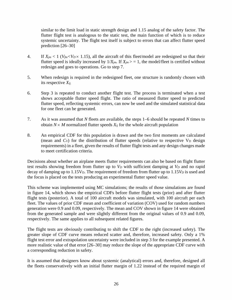
Decisions about whether an airplane meets flutter requirements can also be based on flight flutter test results showing freedom from flutter up to VD with sufficient damping at VD and no rapid decay of damping up to 1.15VD. The requirement of freedom from flutter up to 1.15VD is used and the focus is placed on the tests producing an experimental flutter speed value. This scheme was implemented using MC simulations; the results of those simulations are found in figure 14, which shows the empirical CDFs before flutter flight tests (prior) and after flutter flight tests (posterior). A total of 100 aircraft models was simulated, with 100 aircraft per each fleet. The values of prior CDF mean and coefficient of variation (COV) used for random numbers generation were 0.9 and 0.09, respectively. The mean and COV shown in figure 14 were obtained from the generated sample and were slightly different from the original values of 0.9 and 0.09, respectively. The same applies to all subsequent related figures. The flight tests are obviously contributing to shift the CDF to the right (increased safety). The greater slope of CDF curve means reduced scatter and, therefore, increased safety. Only a 1% flight test error and extrapolation uncertainty were included in step 3 for the example presented. A more realistic value of that error [26–30] may reduce the slope of the appropriate CDF curve with a corresponding reduction in safety. It is assumed that designers know about systemic (analytical) errors and, therefore, designed all the fleets conservatively with an initial flutter margin of 1.22 instead of the required margin of

27

1.15. This means that the average value of the normalized variable Y is now 0.9*1.22 ≈ 1.1. Figure 15 shows the CDF function of normalized flutter speed distribution in a fleet when models are initially designed with 22% redundancy to compensate for the systemic errors discussed in section 3.4.

Figure 14. CDF of flutter speed before and after flight tests (systemic analysis errors accounted for) with a conservative design and no damage

3.6 CONTRIBUTION OF OTHER SAFETY MEASURES

In compliance with section 5.3, Detail Design and Notch Sensitivity, of Policy Statement PS-ACE100-2001-006 [31], some factors may be applied that lead to design values that are lower than base material properties, including the stiffness requirements (flutter or vibration margins). As data on stiffness parameters scatter for composites are available in CMH-17 [24], proper design values similar to the A/B-basis used for failure stress may be derived. The derivation of A-basis value for typical data on composite elastic moduli, described by Weibull PDF with COV = 8%, leads to a stiffness reduction factor of 0.77. The parametric analysis of the composite vertical tail/rudder system described in section 4.2 shows that such a factor results in a flutter speed margin of about 15% above the usual factor of 1.15 in that case. This value of the additional flutter speed margin for composite structures is used in the present study for the evaluation of the POF. 3.7 THE POF

The considerations, assumptions, and statistics discussed in section 3.6 can now be applied to the evaluation of the POF due to flutter. It is first assumed that there is no significant time-dependent structural degradation per structural life, meaning that no material degradation with time or damages are assumed. Therefore, the posterior Xij simulation results shown in figure 13 can be used.

28

Because the failure event is defined here as flight speed exceeding the Xij, and the probability that flight speed does not exceed Xij is described by Gumbel CDF, the probability of exceeding the Xij for individual aircraft in the population is:

1.15*

1 exp exp ijF i

XP

−µ = − − − β

(21)

From equation 14, µ = 1; β = 0.0063 for the flaps-up configuration. The average of this random value over the entire population would be the integral measure of safety against flutter. It also would be consistent to consider the flaps-down flight segment. The maximum speeds for the flaps-down configuration are described by equation 15, with parameters µ = 1; β = 0.039. Let it be assumed that the aircraft structures in all fleets are perfectly optimized for speed margin of 15% plus an additional factor of 1.15 for the elevated stiffness scatter of composite materials. Table 4 shows the probability of flutter failure of metallic and composite aircraft calculated based on analysis only and on analysis supported by flight test results. It also shows the effect on the probability of flutter failure of using nominal and reduced material stiffness data. Instead of the reduced material stiffness data, this probability may be reduced by specifying the elevated flutter speed margin for composite structures. The POF for a margin of 25% instead of 15% is calculated and presented in table 4.

29

Table 4. Probability of flutter failure of metallic and composite aircraft calculated based on analysis only and on analysis supported by flight test results

Metal structure: model mean COV = 9%, Fleet articles COV = 4% Test extrapolation: CV = 1%

Analysis only Analysis Supported by Flight Tests

Mean Y CV % POF, flaps retracted

POF, flaps extended Mean Y CV %

POF, flaps retracted

POF, flaps extended

Unconservative Design 0.9 8.7 0.33 0.45 1.033 5.3 9.9E-4 0.025 Conservative Design 1.099 0 0.012 0.031 1.113 8.7 4.4E-4 0.007

Composite structure: model mean COV = 9%, Fleet articles CV = 6% Test extrapolation: CV = 1%

Analysis only Analysis Supported by Flight Tests

Mean Y CV % POF, flaps retracted

POF, flaps extended Mean Y CV %

POF, flaps retracted

POF, flaps extended

Unconservative Design 0.9 10 0.44 0.45 1.042 8.1 0.017 0.05 A-allowable for stiffness 1.15 2 0.01 0.03 1.16 10 0.0026 0.013 Design for 1.25 flutter factor, Mean Y~1.25VD 0.9 9 0.1 0.22 1.03 5 3.81E-6 0.0078

30

In view of the data contained in table 4, it may be concluded that the flutter flight test is an efficient safety measure that reduces the uncertainty in analytical models; eventually, it helps to shrink the scatter of flutter speeds in a global aircraft population. In most important cases, if a flutter flight test is conducted, this leads to a 100 times reduction of the POF. Wind tunnel flutter tests contributed to the assessment of systemic analysis errors as part of the numerical modeling effort leading to the design of the flutter and flight flutter test. An unconservative design with flight tests provides the minimum dispersion of flutter speed at minimum extra weight. Introduction of a reduced stiffness A-basis allowable is efficient, but not a sufficient safety measure. The more adequate safety measure seems to be increasing the aeroelastic stability margin for composite structures to 25%. The empirical CDF for this case is shown in figure 15. It is emphasized that this conclusion is limited to the studies based on the assumptions presented in this study and that more complete and realistic data may lead to different conclusions by using the present methodology. The posterior CDF shown in figure 15 will be used for POF calculations for composite structure subject to possible damage.

Figure 15. CDF of flutter speed with a margin of 1.22; unconservative design

3.8 PROBABILITY OF FLUTTER FAILURE WITH CHANGES OF AIRFRAME DYNAMIC PROPERTIES OVER TIME

All estimates of probability of flutter failure obtained in section 3.7 were based on the assumption that the structural properties contributing to aeroelastic stability were unchanged over the airplanes’ time of operation. This assumption is supported by modal tests of aircraft in operation and modal tests conducted during fatigue testing in the laboratory. The most important parameters

31

that change with time or use on metal structures mentioned in Selikhov, et al. [15] are structural damping, dry friction, and certain parameters of the control system. Structural damping can usually increase from 1.2–1.3 times per life because of the loosening of joints. Increased free play of control surfaces due to joint wear has been identified as a cause of LCO. The dynamic properties of control surfaces, high lift devices, landing gear, and other similar actuated structural components vary noticeably with time during operations due to general loosening of joints between parts, non-aerodynamic repair of lightweight honeycomb structures, and hinge wear. As composite materials are becoming more widely used in primary structures, three major concerns have been raised in the literature: (1) stiffness degradation due to impact damage (localized or spread), (2) material aging and mass property changes due to environmental exposure and water absorption, and (3) mass property and stiffness changes due to repair. These may be rather substantial, especially for control surfaces. 3.9 FLUTTER PROBABILITY FORMULATION ALLOWING FOR MATERIAL DEGRADATION, ENVIRONMENTAL EFFECTS, INSPECTION PROCEDURES, DAMAGE, AND REPAIR

Similar to the approach used in damage tolerance, an airframe that sustains damage or has seen material degradation will have a residual flutter speed that may be lower than its original flutter speed. The assessment of the POF for residual flutter speed history (accounting for damage and repair during the lifetime of the system) is shown schematically in figure 16. As the figure shows, damage to the structure and subsequent repairs may lead to changes in local stiffness, mass, and linear flutter speed. Damage statistics covering damage size, damage type, damage time of appearance, and duration before repair (depending on maintenance procedures) are converted to a history of residual flutter speed variations. Combined with statistics of flight speeds attained by aircraft in service, it is now possible to assess the probability that some flight speed attained might reach the flutter speed of a damaged or repaired structure. Therefore, the POF due to flutter can now be evaluated. Assuming some structural component or system has the following residual flutter speed history—an initial flutter speed of the new system equaling 1.15VD. Then, at the instant t0 = 0.4 impact damage occurs (e.g., due to hailstorm), the flutter speed is decreased to the value of 1.075VD. As some impact damage may be almost invisible, this damage is not detected until the time instant t1

= 0.6, when the damage is repaired but the flutter speed is restored only partially to a value of 1.1VD due to changes of mass properties (e.g., honeycomb trailing edge). There are three time intervals ti (e.g., 0, 0.4, and 0.6) of constant flutter speed for the system and failure may happen when the occurrence of flight air speed exceeds the critical residual flutter speed at some point during the life of the vehicle. Simple calculations are included in figure 16. The final POF is equal to one minus the product of probabilities that failure does not happen in each of three intervals. In calculating the POF in each of the time intervals, an account is taken of flight speed statistics, residual flutter speed, and the duration of the interval.

32

Figure 16. POF accounting for the possibility of damage and repair

Next, a more realistic case is considered. When the number of damages per life is more than one, there may be several different types of damage (e.g., through-crack, indentation, delamination, disbonding, etc.), damages occurring at random times, and different random sizes. There may also be several different types of inspection methods used (e.g., pre-flight visual inspection and maintenance inspection using different techniques). The time of damage existence (damage life) depends on the frequency of inspections and the capability of inspection to detect damage. Finally, the aeroelastic properties may also change because of material aging and water absorption. Figure 17 shows one history of random damage size versus time, simulated using the MC method. Two types of damage are considered: delamination (solid black line) and hole (grey). The damage size realization can be converted (via residual stiffness assessment) into residual flutter speed realization, and the POF then calculated similar to the manner shown in figure 16.

33

Figure 17. Probability of flutter failure Showing effects of delamination, holes, material degradation, and repair

The POF is assessed based on the simulation of random histories of damage size and time throughout the life of a structure. Each history consists of a number of constant damage size intervals. The starting time of each interval is a random value and the length is a random function of the probability of damage detection (depending on detection methods used and the training of inspection professionals) and inspection frequency. Histories may be randomly simulated using a finite set of primitive random variables, such as damage occurrence rate and probability of damage detection. The damage size may be converted into the appropriate random residual stiffness and then to residual flutter speed, where the reduction of the stiffness occurs due to the presence of both manufacturing defects and accidental operational damage. In addition to stiffness, mass properties may be changed as a result of repair. The MC damage generation module interrogates basic random variables: the number, type, and size of damage and defects; the time of damage initiation; number of inspections to detect damage; initial and residual stiffness as a function of damage size; stiffness/mass after repair; and maximum flight speed within constant damage size interval. Temperatures and temperature/humidity effects can also be added. Using the automated flutter simulation tools described in section 3.3, the resulting flutter speeds are determined and used to evaluate the POF. Current models and simulation capabilities developed at the University of Washington are able to handle any number of defects/damages (upper limit is specified by user), various types of damages,

34

inspections and monitoring, non-uniform inspection schedules, and various maintenance decisions for detected damage repair. 4. PROBABILISTIC 3D PROBLEMS

4.1 THE FIGHTER WING/FLAP CONFIGURATION

4.1.1 Problem Definition

A 3D example of a composite wing with control surfaces (figure 18) is used to demonstrate the ability of the new reliability assessment system.

Figure 18. The fighter wing/control surface configuration

The following input data are used: • Number of Design Cases = 1; Subsonic Flight • Number of Damage Types = 2; Hole and Delamination • Number of Inspection Types = 2; Visual and Instrumental The CDF of maximum flight speed per life (50,000 flight hours) is expressed by equation 14. The probability of structural temperature exceedance is taken from table 8-5 of Ushakov, et al. [32] for cruise subsonic flight. The exceedance data of damage occurrence are taken from Huang, et al. [33] and recalculated for 50,000 flight hours and an applicable panel area. The corresponding graph is shown in figure 19.

35

Figure 19. Damage exceedance data (lear fan 2100 [23])

The log-odds probability of damage detection model described by equation 22 is used with parameters shown in table 5. Figure 20 shows the probability of damage detection for visual and tap hammer inspection methods.

ln( )( )

ln( )1

aePOD a

ae

α + β=

α + β+ (22)

Table 5. Probability of damage detection

Inspection Method α β Visual 4.22 4.69 Tap Hammer -0.55 2.86

36

Figure 20. Probability of damage detection for different inspection methods

It was assumed that the CDF of flutter speed for a new structure was a normal distribution, with parameters shown in figure 15. To obtain the residual flutter speed for the damaged structure, the ABAQUS commercial finite element software package was used to predict the reduction of effective skin stiffness due to damage. Skin panels were simulated as rectangular plates. The load pattern and boundary conditions were chosen to be the same for the panel as it appears in the NASTRAN model of the airframe for natural vibration mode calculations. More refined models of individual panels can be used for finer modeling of the localized damage effect. Panel numbers for panels on the flaperon are shown in figure 21.

Figure 21. Flaperon skin panels (lower surface numbers are in parentheses)

Stiffness reduction for the panel has been estimated as a difference of average relative displacements of opposite nodes per given loading depending on damage size. The damage was assumed in a center of the panel.

37

The analysis has shown that, in general, the residual stiffness may be determined using expressions based on a rule-of-mixtures for constant thickness panel:

( ) ( )

( ) ( )

( )

( )

D DT T U T D

D DC C U C D

W W Wa

W WW W W

bW W

−= +

−= +

κ κ κ

κ κ κ (23)

where: W is the total cross-section width of a panel, W = 450 mm WD is the maximum cross-section of damage size normal to the direction of the applied load κT(U) is the original tensile stiffness of the composite κT(D) is the tensile stiffness of the damage region, which is negligible for hole κC(U) is the original compressive stiffness of the composite κC(D) is the compressive stiffness of the damage region, which is negligible for hole The stiffness reduced in compliance with equation 23 was substituted into the NASTRAN model and, after that, into the ZAERO model to obtain the residual flutter speed. An important possibility that was also taken into account was that the skin can completely fail under the load of horizontal flight corresponding to residual strength at a damage size of about 130 mm. The results are shown in figure 22 for the most flutter-sensitive panels 11, 12, 15, and 16. An aging knockdown factor used is shown in figure 23.

Figure 22. Residual flutter speed vs. damage size for most stiffness-critical panels

38

Figure 23. Aging knockdown factor

A flutter speed repair recovery factor is shown in figure 24. The data used for the figure were obtained by sensitivity analysis for the flaperon model with respect to various panel mass increases due to repair. The rear part of the flaperon was assumed to be honeycomb structure and conservative assumptions were made: (1) for damage size from zero to 38 mm, the weight gain is equal to the weight of the round cylinder between the skins of diameter equal to the damage size made of epoxy, (2) for the damage size from 38–200 mm, weight gain is the weight of a ring between the skins of diameter equal to the damage size, 25 mm-thick, and made of epoxy, and (3) for the damage size more than 200 mm, the flaperon is replaced (no weight gain). It was assumed the temperature does not affect the flutter speed.

Figure 24. Flutter speed repair recovery knockdown factor for different panels

4.1.2 Results for the Fighter Type Wing

With the data obtained, the POF could be calculated. Figure 25 shows the POF due to damage in panel 15 versus safety margins. Six flaperon panels—11, 12, 15, 16, 19, and 20—were found to significantly influence the flutter POF. The POF without damages is also shown for comparison.

39

Figure 25. Probability of flutter failure due to panel 15 vs. safety margin accounting and not accounting for damage

The probabilistic analysis shows that to ensure the same POF as in a no-damage case (where a margin of 1.22 was used for conservative design), the speed safety margin with nominal stiffness should be increased by about 0.07–0.08VD. It should be emphasized that this conclusion is case-dependent and limited to the test case studied for this report. The MC method used here allows one to also analyze the circumstances of possible flutter failures. In the example problem, the majority of flutter occurrences happened after static failure with complete loss of skin stiffness on damaged panels. The characteristic time of operation with such damages is one flight because such damage will be detected by technicians on the ground. Only big delamination failures may be missed. Therefore, in such cases, when flutter due to damage is only associated with complete loss of stiffness of skin panels, the probability of secondary failure practically depends on inspection interval. The latter should be established on the basis of reliability analysis for residual strength considerations, which will also account for flutter. For some airframe designs, situations may occur where damage or a combination of damages that lead to partial local loss of stiffness or increased mass may lead to flutter failures. The simulation capabilities developed for this work, and described in section 3.3 can be used to predict flutter failure and to apply the findings for design and maintenance. 4.2 THE UNCERTAIN AEROELASTIC COMPOSITE VERTICAL TAIL/RUDDER SYSTEM

4.2.1 The Model

A realistic NASTRAN model of a composite vertical tail/rudder system of a passenger airplane (but not one representing any actual flying vehicle) is shown in figure 26. Generally, flutter analysis and certification of tail surfaces is carried out for the coupled tail/empennage or tail/aircraft system to account for the effect of fuselage motion and root conditions on the flutter

40

speed, but for the exploratory study presented in this report, the nodes at the root end of the spars were fixed.

Figure 26. Representative composite vertical tail/rudder FEA model

The tail structure is assembled from several separately manufactured panels. Thus, panel-to-panel variability should be considered. Properties of structural subcomponents manufactured separately are assumed to be independent. As each panel is divided into FEs, the element-to-element variability should be accounted for as well. The properties of individual FE skin panels, spars, stringers, and frames FEs are assigned appropriately. The properties of the neighboring elements are closely correlated and this should be properly considered. Some probabilistic aeroelastic studies to date involve simple aeroelastic models such as beam-like wings, with the spatially distributed uncertainties considered in a form of Markov field. The covariance kernel of the random field is often assumed in the form:

1| |

21( , ) cor

x x

RpC x x e

− −

= σ (24) where σp2 is a field variance and Rcor is a radius of correlation. This model is used in this report. The model random input is characterized by the variability data shown in Table 6 (PSHELL element properties). The typical C.O.V. values of Table 6 parameters were taken from CMH-17. Theoretically, the radius of correlation could also have been evaluated from the data of the CMH-17 had the appropriate supporting information—such as panel size and coupon size—been present. The C.O.V. of thickness and Young’s modulus for PBAR and PROD properties were assumed to be equal to 0.02. The same value has been used for CONM2 mass elements. The NASTRAN model of the system was modified to allow every structural and mass element to have its own property and material card. The elements belonging to structural panels which are manufactured separately were united into groups to represent panel-to-panel variability.

41

Table 6. Variability data for the composite tail/rudder system (PSHELL element

properties)

Property

Panel-to- panel

C.O.V.

Element-to- element C.O.V.

Radius of Correlation,

in. Thickness t 0.03 0.01 10 G11 0.05 0.02 100 G12 0.05 0.02 100 G22 0.05 0.02 100

Attention was paid to adequate simulation of the composite skin panels where impact damages were expected. Those structural panels were simulated using NASTRAN SHELL Fes, listed in table 7, with randomized thickness and three random material properties: G11, G12, and G22. Since the example FE model arrived with lumped masses representing mass distribution for dynamics purposes, the material density was simulated as included in those lump masses. The correlation between local thickness and structural mass of each FE was not simulated because of the lack of appropriate information for this particular model. Average panel geometric and materials properties were simulated independently, while those of individual FE belonging to each panel were simulated using the Markov random field.

Table 7. The NASTRAN FE model of the composite tail/rudder system

Number of grid points 1,268 Number of CBAR elements 309 Number of CBUSH elements 45 Number of CONM2 elements 28 Number of CQUAD4 elements 1,409 Number of CROD elements 1,056 Number of CSHEAR elements 91 Number of CTRIA3 elements 187 Number of RBE2 elements 16 Number of RBE3 elements 28

Figure 27 shows the aerodynamic model used for the vertical tail rudder system. The unsteady aerodynamics are based on the Doublet Lattice Method (although, as previously stated, ZAERO has also been used in the automated flutter simulation capability). The aerodynamic reference surface on the plane x-z is divided into five trapezoidal macropanels. Each macropanel is subdivided into strips of trapezoidal panels. Surface splining for information transmission between structural and aerodynamic points is handled by NASTRAN. In this model, trapezoidal surfaces 1, 2, and 3 have the same number of aerodynamic elements in the wing span direction. Similarly, surfaces 4 and 5 have the same number of aerodynamic elements in the wing span direction. The

42

root of the structural FE model of the vertical tail was not exactly parallel to the axis of the incoming flow. The aerodynamic reference surface was slightly adjusted to align the root with the x direction.

Figure 27. Vertical tail/rudder system: aerodynamic model (doublet lattice method) showing the number of spanwise and chordwise aerodynamic box divisions for each large

panel

4.2.2 Results for the Composite Vertical Tail/Rudder System

Figures 28 and 29 show the free vibration mode shapes of the nominal structure, with natural frequencies close to flutter frequency of about 13 Hz. The automated flutter simulation capability produces mode shapes and natural frequencies efficiently for any variation of the aeroelastic system analyzed. Carrying out structural dynamic and flutter simulations of large numbers of variants of the aeroelastic system analyzed is referred to as virtual tests. Actual natural modes contributing to the flutter mechanism vary depending on alternatives in the structure and possible switching of flutter mechanisms depending on the magnitude and combination of structural changes.

43

Figure 28. Free vibration mode shape of the nominal structure, frequency = 16.34 Hz

Figure 29. Free Vibration Mode Shape of the Nominal Structure, Frequency = 18.24 Hz.

The most interesting results of the virtual flutter tests are shown in figures 30 and 31. Figure 30 shows the empirical CDF of the flutter velocity. It is obvious that the corresponding PDF is bimodal. This fact is shown in the corresponding histogram in figure 31. This essentially means that some aircraft simulated in a fleet using the assumptions in this analysis may have flutter mechanisms significantly different from those in the main population. It is also evident that the variance of the second flutter mechanism is much smaller than the first one. This may represent evidence of different uncertainty propagation for different failure modes. In this particular case, the second mode of PDF is on the right steep branch of CDF, which does not contribute much to the POF. There may be situations when this mode appears on the left tail. It is also evident that some popular fast reliability methods, such as SORM and FORM [34], may generally not be applicable to the probabilistic study of flutter and similar aeroelastic phenomena.

44

Figure 30. CDF for vertical tail flutter felocity (no damage)

Figure 31. Flutter velocity histogram (no damage)

Another observation is that the variance of Vf is noticeably greater than variances for input parameters shown in table 6. This is not a general conclusion and seems, again, to be case-dependent because earlier studies using a simple delta wing model led to different distribution characteristics. The results presented in this report, accordingly, serve to demonstrate the methodology and capability of the probabilistic flutter reliability assessment system presented and

45

not to draw any general conclusions regarding the reliability of particular aeroelastic systems types. Figure 32 shows that the empirical CDF of the flutter speed Vf obtained with the virtual aeroelastic testing module (VATM) of the tail torsion box skin has large damage size of about 150 mm. During the simulation, a randomly selected element was used to produce the CDF. The no-damage test case was also plotted for comparison purposes. Only stiffness reduction due to damage was considered and estimated by using analysis of the element itself as the difference of average relative displacements of opposite nodes per given loading depending on damage size. The damage was assumed at a center of the element. The locations of damaged elements have been chosen randomly with uniform distribution over the tail box skin area.

Figure 32. Empirical CDF of Vf for the damaged and undamaged structure

As in Lin [2], for the exploratory studies presented in this report, the residual panel stiffness has been determined using expressions based on a rule-of-mixtures for constant thickness panel equation 23. The cross-section width of an element has been defined for each randomly selected element in the direction coinciding with an aircraft longitudinal axis at the position of element centroid. The Vf CDF for the undamaged structure is shown in figure 32 for comparison. The average values are almost the same, but the C.O.V. of the damaged structure is much greater. This behavior is rather different from the derived results of previous studies using a simple delta wing model [35] in which the average decreased with the damage size but the C.O.V. remained nearly constant. Both behaviors will inevitably lead to lower reliability.

46

4.2.3 Flutter Reliability of Damaged and Undamaged Composite Airframes

The methodology and capabilities described in this section are used to compare flutter failure reliability of undamaged and damaged composite airframes, particularly in the case of the tail/rudder example presented in section 4.2.2. Input data for the University of Washington’s Reliability Life-Cycle Analysis of Composite Structures [2] were taken from [33, 36, 37]. Panel weight change due to repair was not considered because of the lumped mass nature of both structural and nonstructural mass in the model provided for this work by industry. The Vf CDF for undamaged structure and damaged structure were taken by polynomial approximation of curves shown in figure 32 and other curves obtained with the virtual aeroelastic testing capability for different damage sizes.

The following input data were used:

• Number of Design Cases = 1; Subsonic flight

• Number of Damage Types = 2; Hole and delamination

• Number of Inspection Types = 2; Visual and instrumental

• The CDF of maximum flight speed per life is expressed by equation 14 (see also equation

3 in [33])

• The probability of damage detection model described in [2] was used

• The exceedance data of damage occurrence is taken from [32] and recalculated for 60,000 flight hours and torsion box skin area. To introduce even more conservatism, the damage sizes in the calculations were two times larger than those in [32]. This might include the damages inflicted by uncontained turbine blades and similar cases

Figure 33 shows the POF in flutter accounting for damage depending on the safety margins used for design. The POF without damages as a function of the safety margin used for design is also shown for comparison.

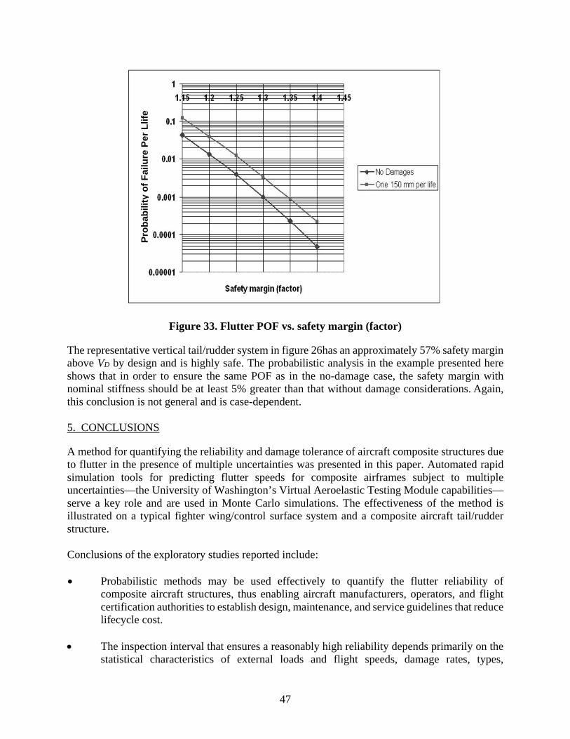
47

Figure 33. Flutter POF vs. safety margin (factor)

The representative vertical tail/rudder system in figure 26has an approximately 57% safety margin above VD by design and is highly safe. The probabilistic analysis in the example presented here shows that in order to ensure the same POF as in the no-damage case, the safety margin with nominal stiffness should be at least 5% greater than that without damage considerations. Again, this conclusion is not general and is case-dependent. 5. CONCLUSIONS

A method for quantifying the reliability and damage tolerance of aircraft composite structures due to flutter in the presence of multiple uncertainties was presented in this paper. Automated rapid simulation tools for predicting flutter speeds for composite airframes subject to multiple uncertainties—the University of Washington’s Virtual Aeroelastic Testing Module capabilities—serve a key role and are used in Monte Carlo simulations. The effectiveness of the method is illustrated on a typical fighter wing/control surface system and a composite aircraft tail/rudder structure. Conclusions of the exploratory studies reported include: • Probabilistic methods may be used effectively to quantify the flutter reliability of

composite aircraft structures, thus enabling aircraft manufacturers, operators, and flight certification authorities to establish design, maintenance, and service guidelines that reduce lifecycle cost.

• The inspection interval that ensures a reasonably high reliability depends primarily on the

statistical characteristics of external loads and flight speeds, damage rates, types,

Pro

babi

lity

of F

ailu

re P

er L

life

48

inspection, and repair as well as residual static strength and stiffness of the damaged structure.

• The most uncertain variables in any probabilistic damage-tolerance design method are damage size and frequency. To obtain in-service data that contain complete descriptions of damage size and frequency, structural damage locations, inspection methods, and repairs used are important but remain a major challenge.

• Additional studies of different structural airframe configurations are required—in

particular, horizontal tail/elevator/tab systems, wing/control surface systems, and complete aircraft. Effects of hinge failure and possible failure of internal structure should also be considered. Other modes of failure due to aeroelastic behavior, such as dynamic stresses due to gust excitation and fatigue effects of limit cycle oscillations, should also be studied. The methodology presented here and the associated simulation tools can be extended to cover all such cases in addition to the effects of aerodynamic and control system (actuator) uncertainties

6. REFERENCES

1. Pettit, C.L., “Uncertainty Quantification in Aeroelasticity: Recent Results and Research Challenges,” Journal of Aircraft, Vol. 41, No. 5, 2004, pp. 1217–1229.

2. Lin, K.Y., Styuart, A., “Development of Reliability-Based Damage Tolerant Structural Design Methodology,” 47th AIAA/ASME/ASCE/AHS/ASC Structures, Structural Dynamics, and Materials Conference, Paper 2006-2156, Newport, Rhode Island, May 1–4, 2006.

3. Tang, D.M., Dowell, E.H., Virgin, L.N., “Limit Cycle Behavior of an Airfoil With a Control Surface,” Journal of Fluids and Structures, Vol. 12, No. 7, 1998, pp. 839–858.

4. Pettit, C.L., Beran, P.S., “Effects of Parametric Uncertainty on Airfoil Limit Cycle Oscillations,” Journal of Aircraft, Vol. 40, No. 5, 2004, pp. 1217–1229.

5. Saltelli, A., Chan, K., Scott, E.M., Sensitivity Analysis, John Wiley & Sons, Chichester, New York, 2000.

6. Schaeffer, H.G., MSC.NASTRAN Primer for Linear Analysis, 2nd edition, MSC Software, Santa Ana, California, 2001.

7. ZAERO, Engineers’ Toolkit for Aeroelastic Solutions, ZONA Technology, Inc., Scottsdale, Arizona, 2004.

8. Livne, E., “Integrated Aeroservoelastic Optimization: Status and Progress,” Journal of Aircraft, Vol. 36, No. 1, January–February 1999, pp. 122–145.

9. Roger, K.L., “Airplane Math Modeling Methods for Active Control Design,” Structural Aspects of Active Controls, AGARD CP-228, August 1977, pp. 4–11.

49

10. Karpel, M., “Design for Active Flutter Suppression and Gust Alleviation Using State Space Aeroelastic Modeling,” Journal of Aircraft, Vol. 19, No. 3, March 1982, pp. 221–227.

11. Mor, M., Livne, E., “Minimum State Unsteady Aerodynamics for Aeroservoelastic Configuration Shape Optimization of Flight Vehicles,” AIAA Journal, Vol. 43, No. 11, November 2005, pp. 2299–2308.

12. Mor, M., Livne, E., “Sensitivities and Approximations for Aeroservoelastic Shape Optimization with Gust Response Constraints,” Journal of Aircraft, Vol. 43, No. 5, September–October 2006, pp. 1516–1527.

13. Mor, M., Livne, E., “Minimum State Unsteady Aerodynamic Shape Sensitivities Using Sensitivity of Optimal Solutions to Problem Parameters,” AIAA Journal, Vol. 45, No. 9, 2007, pp. 2187–2195.

14. Karpel, M., “Sensitivity Derivatives of Flutter Characteristics and Stability Margins for Aeroservoelastic Design,” Journal of Aircraft, Vol. 27, No. 4, 1990, pp. 368–375.

15. Selikhov, A.F., Chizhov, V.M., “Probabilistic Methods in Structural Strength Analysis,” Mashinostroenie Publishing House, Moscow, 1987 (in Russian).

16. Taylor, J., “Manual on Aircraft Loads,” Published for and on behalf of the Advisory Group for Aeronautical Research and Development, North Atlantic Treaty Organization by Pergamon Press, Oxford, New York, 1965.

17. Styuart, A.V., Chizhov, V.M., Legnyov, M.Y., “Extrapolation of Load Exceedance Curves for Estimation of Probability of Aircraft Structural Failure,” Tekhnika Vozdushnogo Flota, No. 6, Moscow, 1998 (in Russian).

18. Rustenburg, J., Skinn, D., Tipps, D.O., “Statistical Loads Data for Boeing 737-400 in Commercial Operation,” FAA Report DOT/FAA/AR-98/28, August 1998.

19. Tipps, D.O., Rustenburg J., Skinn, D., “Statistical Loads Data for Boeing 767-200ER in Commercial Operation,” FAA Report DOT/FAA/AR-00/10, March 2000.

20. Rustenburg, J., Skinn, D., Tipps, D.O., “Statistical Loads Data for Bombardier CRJ100 Aircraft in Commercial Operation,” FAA Report DOT/FAA/AR-03/44, June 2003.

21. Skinn, D., Tipps, D.O., Rustenburg, J., “Statistical Loads Data for Md-82/83 Aircraft in Commercial Operations,” FAA Report DOT/FAA/AR-98/65, February 1999.

22. Rustenburg, J., Skinn, D., Tipps, D.O., “Statistical Loads Data for the Airbus A-320 Aircraft in Commercial Operation,” FAA Report DOT/FAA/AR-02/35, April 2002.

23. Acar, E., Kale, A., Haftka, R.T., Stroud, W.J., “Structural Safety Measures for Airplanes,” Journal of Aircraft, Vol. 43, No. 1, January–February 2006.

24. Composite Materials Handbook-17 https://www.cmh17.org/

50

25. Styuart, A., Mor, M., Livne, E., Lin, K., “Risk Assessment of Aeroelastic Failure Phenomena in Damage Tolerant Composite Structures,” AIAA Paper 2007–1981, 48th AIAA/ASME/ASCE/AHS/ASC Structures, Structural Dynamics, and Materials Conference, Honolulu, Hawaii, April 23–26, 2007.

26. Brenner, M.J., “Aeroservoelastic Uncertainty Model Identification From Flight Data,” NASA TM 2001-210397, July 2001.

27. Cooper, J.E., “Towards Faster and Safer Flight Flutter Testing,” Chapter 43, RTO MEETING PROCEEDINGS 89, “Reduction of Military Vehicle Acquisition Time and Cost Through Advanced Modelling and Virtual Simulation,” Papers presented at the RTO Applied Vehicle Technology Panel (AVT) Symposium, Paris, France, April 22–25, 2002, Published March 2003.

28. Pickrel, C.R., White, P.J., “Flight Flutter Testing of Transport Aircraft: In-Flight Modal Analysis,” Proceedings of IMAC 21, The International Modal Analysis Conference, Kissimmee, Florida, 2003.

29. Mevel, L., Goursat, M., Benveniste, A., Basseville, M., “Aircraft Flutter Test Design Using Identification and Simulation: a SCILAB Toolbox,” Proceedings of 2005 IEEE Conference on Control Applications, Toronto, Canada, August 28–31, 2005, pp. 1115–1120.

30. Heeg, J., “Stochastic Characterization of Flutter Using Historical Wind Tunnel Data,” AIAA 2007-1769, 48th AIAA/ASME/ASCE/AHS/ASC Structures, Structural Dynamics, and Materials Conference, Waikiki, Hawaii, April 23–26, 2007.

31. Policy Statement PS-ACE100-2001-006, FAA, December 21, 2001.

32. Ushakov, A., Stewart, A., Mishulin, I., Pankov, A., “Probabilistic Design of Damage Tolerant Composite Aircraft Structures,” FAA Report DOT/FAA/AR-01/55, January 2002.

33. Huang, C., Lin, K.Y., “A Method for Reliability Assessment of Aircraft Structures Subject to Accidental Damage,” 46th AIAA/ASME/ASCE/AHS/ASC Structures, Structural Dynamics and Materials Conference, AIAA-2005-1830, Austin, Texas, April 18–21, 2005.

34. NESUUS Theoretical Manual, Southwest Research Institute, Version 7.0, October 2001.

35. Styuart, A., Demasi, L., Livne, E., Lin, K., “Probabilistic Modeling of the Aeroelastic Life Cycle for Risk Evaluation of Composite Structures,” AIAA-2008-2300 49th AIAA/ASME/ASCE/AHS/ASC Structures, Structural Dynamics, and Materials Conference, Schaumburg, Illinois, 2008.

36. Gary, P.M., Riskalla, M.G., “Development of Probabilistic Design Methodology for Composite Structures,” Vought Aircraft Company, FAA Report DOT/FAA/AR-95/17, August 1997.

51

37. Lin, K.Y., Du, J., Rusk, D.T., “Structural Design Methodology Based on Concepts of Uncertainty,” National Aeronautics and Space Administration, Report CR-2000-209847, Langley, Virginia, February 2000.