WIDER Working Paper 2016/88

Anti-corruption policy-making, discretionary power, and institutional quality

An experimental analysis

Amadou Boly1 and Robert Gillanders2

July 2016

1 African Development Bank, Abidjan, Côte d’Ivoire, corresponding author: a.boly@afdb.org; 2 Hanken School of Economics, Helsinki, Finland, rgillanders@gmail.com.

This study has been prepared within the UNU-WIDER project on ‘Macro-Economic Management (M-EM)’.

Copyright © UNU-WIDER 2016

Information and requests: publications@wider.unu.edu

ISSN 1798-7237 ISBN 978-92-9256-131-4

Typescript prepared by Sophie Richmond.

The United Nations University World Institute for Development Economics Research provides economic analysis and policy advice with the aim of promoting sustainable and equitable development. The Institute began operations in 1985 in Helsinki, Finland, as the first research and training centre of the United Nations University. Today it is a unique blend of think tank, research institute, and UN agency—providing a range of services from policy advice to governments as well as freely available original research.

The Institute is funded through income from an endowment fund with additional contributions to its work programme from Denmark, Finland, Sweden, and the United Kingdom.

Katajanokanlaituri 6 B, 00160 Helsinki, Finland

The views expressed in this paper are those of the author(s), and do not necessarily reflect the views of the Institute or the United Nations University, nor the programme/project donors.

Abstract: We analyse policy makers’ incentives to fight corruption under different institutional qualities. We find that ‘public officials’, even when non-corrupt, significantly distort anti-corruption institutions by choosing a lower detection probability when this probability applies to their own actions (legal equality), compared to a setting where it does not (legal inequality). As ‘public officials’ are on average equally corrupt with or without legal equality, an institutional setting with legal equality can be considered worse in reducing corruption. Finally, corruption is significantly lower when the detection probability is exogenously set, suggesting that the institutional power to choose detection can itself be corruptive.

Keywords: anti-corruption, embezzlement, experimental economics, institutions, policy-making JEL classification: C91, D02, D73, D81

Acknowledgements: This research project started while Amadou Boly was a Research Fellow at the UNU-WIDER. The views expressed here are those of the author(s) and do not necessarily represent or reflect those of the African Development Bank. We thank the staff at the Busara Center for Behavioral Economics for implementing the experiment. We are grateful to Elizabeth David-Barrett, Michael Breen, and Topi Miettinen for helpful comments and suggestions.

1

1 Introduction

The fight against corruption has resulted in strikingly few success stories (Heeks and Mathisen 2012; Mutebi 2008). While there are many clear practical difficulties in this fight, part of the failure is explicable by the unwillingness of some governments to try to eliminate or even curb corruption (Fritzen 2005). This is most likely to be a problem in weak institutional environments where the policy makers are themselves corrupt. A key issue in the fight against corruption is that ‘anticorruption strategies are adopted and implemented in cooperation with the very predators who control the government and, in some cases, the anticorruption instruments themselves’ (Mungiu-Pippidi 2006: 87).

This paper describes the results of a framed laboratory experiment designed to analyse incentives to fight corruption under different institutional settings. The basic design of our repeated-game experiment is as follows. In the control treatment, in each round, two randomly matched public officials, A and B, are entrusted with separate funds to be spent on (different) social projects. Each public official can embezzle some of the fund under their control. The amounts sent to the social projects are multiplied by 2 while the amounts embezzled by officials A and B are multiplied by 1. Thus embezzlement is socially inefficient. As there is no monitoring and punishment, the control treatment mimics an institutional environment where there is total impunity regarding corruption.

There are three additional treatments with detection and punishment.1 In the first treatment

(Endogenous and Discretionary, ED), Public Official A has the power to choose a level of detection probability, which can take the following values: 0 per cent, 5 per cent, 10 per cent, 15 per cent, 20 per cent, 25 per cent, or 30 per cent. Detection and punishment applies only to Public Official B. This is analogous to a weak institutional environment, with endogenous detection and discretionary punishment institutions; for example, where the judicial and police systems act in the service of the government (as opposed to the state). As a result, opposition leaders are jailed while government supporters are shielded from prosecution. In the second treatment (Endogenous and Non-Discretionary, END), Public Official A is again given the power to choose a level of detection probability but detection and punishment applies both to Public Official A and Public Official B. This situation can also be described as a weak institutional environment, with endogenous detection but non-discretionary punishment institutions, for example, when the judicial and police systems work independently, but under ‘manipulable’ monitoring and punishment institutions. In the third treatment (Exogenous and Non-Discretionary, XND), the probability of detection is set exogenously at 30 per cent and applies to both public officials. This situation reflects a strong institutional environment, with non-discretionary punishment and exogenous detection and punishment mechanisms, for example, a state where the judicial and police systems work independently, under non-discretionary strong punishment laws.

The analyses in this paper focus on choices made by Public Official A. We find that Public Official As choose a weaker, though non-zero, anti-corruption policy in the END treatment when they too are subject to its provisions, compared to the ED treatment where they are not subject to its provisions. Because Public Official As are equally likely to be corrupt in each treatment, the move from ED to END is undesirable from the perspective of reducing overall corruption in the society; given that a lower probability of detection and punishment has been found to increase corruption (Abbink et al. 2002; Schulze and Frank 2003; Olken 2007; Hanna et

1 In case of embezzlement, a detected public official loses both their salary and the amount embezzled.

2

al. 2011). Even a Public Official A, who chooses to be honest in a given experimental round, will choose a weaker anti-corruption policy when it notionally applies to him too. We also find some evidence that corrupt decision makers in the END treatment tend to impose a larger distortion than their corrupt counterparts in the ED treatment, suggesting complementarity between two acts of corruption: embezzlement and institutional distortion. However, it is worth noting that in both the ED and END treatments, the choice of detection probability is significantly different from zero. This suggests that, despite the distortion caused by a weak institutional setting, there is some scope for anti-corruption law-making. The implications of our findings are therefore not entirely pessimistic and they should be of practical value and interest to both domestic and external anti-corruption actors in developing and transition countries. Finally, the level of corruption is found to be significantly lower when detection levels are exogenously set by the experimenter (in the control and XND treatments) compared to the treatments with endogenous detection (ED and END), suggesting that institutional power can be corruptive.

The remainder of this paper proceeds as follows: Section 2 reviews the relevant literature and further motivates our work in its light; Section 3 outlines in full our experimental design; Section 4 presents our results, and Section 5 concludes.

2 Literature review

Our work is related to the sizeable experimental literature that has examined corruption and anti-

corruption policies.2 In particular, our work builds on a literature that investigates the role of

monitoring and punishment. In a seminal bribery experiment, Abbink et al. (2002) show that a small exogenous probability of detection (0.3 per cent) combined with severe punishment (whereby detected subjects are excluded from the experiment without any payment) significantly reduces the likelihood of sending or accepting a bribe. Likewise, in a complex multi-stage embezzlement experiment with endogenous monitoring instead of an exogenous detection probability, Azfar and Nelson (2007) find that monitoring significantly discourages corrupt behaviour. Building on Azfar and Nelson (2007)’s design, Barr et al. (2009) show a relatively strong effect of detection and punishment on corruption. They find that a 44 per cent increase in detection probability leads to a 27 per cent decrease in embezzled resources. Using a natural field experiment in Indonesia, Olken (2007) finds that increasing the audit probability from 4 per cent in the control treatment to 100 per cent reduces embezzlement of project expenditures by an average of 8 per cent, suggesting low economic significance. Overall, these experiments suggest that monitoring and punishment can indeed curb corruption.

However, a few experiments have highlighted possible negative behavioural effects of monitoring and punishment. In particular, Schulze and Frank (2003) conducted an experiment in which the probability of detection increases with the bribe taken. The risk rises from 0 per cent for the lowest bribe to 67 per cent for the two highest bribes. They find that 9.4 per cent of subjects take no bribe in the control treatment (with no monitoring) compared to only 0.9 per cent in the treatment with monitoring and punishment. Additionally, with monitoring and punishment, subjects are more likely to choose the median bribe amount (compared to the lowest and the highest bribes), leading to a higher average bribe. The authors argue that monitoring and punishment deters subjects from the highest bribe levels (due to higher detection levels), but also crowds out intrinsic motivation for honesty or lowest bribe levels. In a one-shot bribery experiment, Serra (2012) finds that traditional monitoring and punishment (with a 4 per

2 A comprehensive and relatively recent review of this literature is provided by Abbink and Serra (2012) while Rocha Menocal et al. (2015) review the broader literature on what works in anti-corruption.

3

cent detection risk) does not curb corruption significantly compared to a no-monitoring treatment. However, combining bottom-up monitoring (whistleblowing) and top-down auditing appears to have a negative effect on bribery. The author advances three possible reasons for this result: fear of social disapproval in the form of citizens’ reports, aversion to betrayal, and/or erroneous attribution of a higher probability of punishment.

Institutional and organizational features have been shown to play a role in determining corruption outcomes. Abbink (2004) finds that staff rotation reduces the frequency of bribery. Relatedly, Schikora (2011) concludes that the ‘four-eyes principle’ actually increases corruption, all else being equal. Azfar and Nelson (2007) find that elected enforcement officers work harder at curbing corruption relative to those who are appointed to the role. Abbink and Ellman (2010) find that the use of intermediaries by aid donors to target beneficiaries can lead to increased embezzlement. Legal asymmetries in punishment for bribers and bribe takers have been studied in terms of collusive and harassment bribery with differing conclusions. Engel et al. (2013) conduct an experiment regarding the former type of bribery and conclude that legal asymmetries increase corruption by giving the briber a credible way to enforce the corrupt transaction. Abbink et al. (2014), however, find that in the context of harassment bribes, legal asymmetry can reduce corruption (though this effect is mitigated by the threat of retaliation). Makowsky and Wang (2015) show that an organization’s shape is important in terms of embezzlement outcomes, in that an increase in the number of tiers is detrimental with regard to this type of corruption.

We contribute to this experimental literature on institutions and corruption in two ways. First, we analyse the problem of elites’ commitment to fighting corruption. This has typically been put aside in the experimental literature on corruption, despite being of prime importance in

successfully fighting corruption (Abbink and Serra 2012).3 Our paper is a step towards better

understanding elites’ incentives to fight corruption. Second, most developing and transition countries are characterized by weak institutional environments. Such an environment has typically been modelled in corruption experiments in a restrictive way, mainly by setting a low

and exogenous detection probability (Abbink et al. 2002; Serra 2012).4 In contrast to previous

studies, we create a richer institutional framework by disaggregating institutional quality into two

concepts in our design—equality before the law and manipulability.5

Equality before the law is the principle that all persons should be treated the same before the law, without regard to wealth, social status, or political power. In weak institutional environments (in particular), equality before the law is unlikely to hold as a result of selective enforcement. Manipulability is the extent to which institutions can be manipulated. The less manipulable institutions are the more stable they can be. The concept of manipulability acknowledges the fact that developing countries are typically characterized by the ability of the elite to deliberately

3 For instance, in their chapter on anti-corruption policies in the lab, Abbink and Serra (2012: 5, 6) discussed strategies to fight corruption specifically abstracting from the problem of a government’s commitment to such a

fight.

4 A notable example of endogenous detection probability is Berninghaus et al. (2013), where the probability of detection falls with the number of corrupt agents. Compared to Azfar and Nelson (2007) and Barr et al. (2009) who also implemented endogenous monitoring, our design is much simpler.

5 Equality before the law and manipulability can be seen as specific aspects of two other concepts—enforcement and stability—used by Levitsky and Murillo (2009) to characterize institutional strength. Enforcement can be defined as the imposition of material, political, or reputational costs on non-compliance with the law. Stability can be defined as the extent to which institutions survive not only the test of time but also changes in the conditions under which they were initially created.

4

manipulate institutions to their advantage (North et al. 2009; Robinson and Acemoglu 2008). The concept of manipulability is thus closely related to the idea of state capture as defined by Kaufmann and Kraay (2002: 30):

State capture is defined as the undue and illicit influence of the elite in shaping the laws, policies and regulations of the state. In its emphasis on the formulation and shaping of laws and regulations of the state, state capture departs from the conventional view of corruption which stresses bribery to influence the implementation of such laws and regulations.

In our experimental framework, the move from ED to END is an improvement along the equality dimension holding manipulability constant. The move from either the control treatment or XND to END constitutes an increase in manipulability, holding equality constant. Moving from any other treatment to END also opens the door to another form of corruption, namely abusing the public power to choose the strength of the anti-corruption policy in order to facilitate one’s own embezzling. In other words, the END treatment allows for state capture.

3 Experimental design

In this section, we start by discussing the experimental procedures, followed by a description of the experimental treatments.

3.1 Procedure

Our framed lab experiment was conducted at the Busara Center for Behavioral Economics in Nairobi, Kenya. The subjects were recruited primarily from the University of Nairobi and came from a variety of study fields. At the beginning of each session, the instructions were read aloud. The subjects then had the opportunity to ask questions. In addition, subjects were also asked to answer some comprehension questions. Each session lasted about one hour.

In our experiment, we model embezzlement, which occurs when the embezzler misuses (typically for private gains) another party’s money or property, to which they have legal access but not legal ownership. Specifically, the experiment is based on a sequential-move game with two players, called Public Official A and Public Official B. Each subject kept the same role throughout the experiment. At the beginning of each round, new pairs (consisting of one Public Official A and one Public Official B) were formed randomly. During the experiment, the payoffs were measured in Experimental Currency Units (ECU). At the end of the experiment, the amount in ECU was converted into Kenyan Shillings at the rate of 8 ECU = 1 KSh.

In each round, both Public Official A and Public Official B receive a salary of 1,140 ECU. In addition, they are both allocated funds amounting to 2,280 ECU, to spend on ‘social projects’. Public Official A, the first mover, must then choose between keeping 0 ECU and keeping 760 ECU from the allocated funds. The amount of ECU that they choose to keep is transferred to their private account. The remainder (2,280 less the amount kept) is multiplied by 2, converted into Kenyan Shillings, and sent to a recipient, called Recipient 1, that is randomly drawn from a list of local non-governmental organizations (NGOs) and local charity funds.

Public Official B makes their decisions only after observing the decisions made by Public Official A. In contrast to Public Official A, Public Official B can keep any whole number between 0 and 2,280 ECU from their allocated funds. The amount that Public Official B chooses to keep is transferred to their private account. The remainder (2,280 less the amount kept) is

5

multiplied by 2, converted into Kenyan Shillings, and sent to a recipient, called Recipient 2 that is different from Recipient 1 and is also randomly drawn from a list of local NGOs and local

charity funds.6

The experiment consisted of 40 independent rounds. In the first 20 rounds, Public Official A receives no information about the choice made by Public Official B. From round 21 onwards, Public Official A was able to observe the amount that was transferred to Recipient 2 by Public Official B. After completing all 40 rounds, all subjects were asked to fill in a questionnaire demographic survey, which included questions on, inter alia, age, gender, monthly expenses, and education.

3.2 Treatments

Our objective is to better understand the workings of detection and punishment as an anti-corruption measure. To do so, we conducted four experimental treatments, three of which include detection and punishment. If a public official’s embezzlement is detected then the public official loses both their salary and the amount embezzled. In the control treatment, Public Official A and Public Official B make their decisions in the absence of any detection and punishment institutions following the game described above.

In the second treatment (ED), Public Official A is given the power to choose a level of detection probability, which can take one of the following values: 0 per cent, 5 per cent, 10 per cent, 15 per cent, 20 per cent, 25 per cent, or 30 per cent. However, detection and punishment institutions apply only to Public Official B, thereby breaking the principle of equality before the law. In other words, Public Official A can be corrupt with impunity while Public Official B faces the prospect of detection and punishment. As a result, detection is endogenously chosen and punishment is discretionary. The choices made by Public Official A relative to embezzlement and the level of detection are observed by Public Official B, before they make their decision. If detected, Public Official B loses both their salary and the amount of social funds embezzled.

In the third treatment (END), Public Official A is again given the power to choose a level of detection probability (from among the values above) but detection and punishment apply both to Public Official A and B. So while the principle of equality before the law is respected, the monitoring and punishment institutions are chosen by Public Official A, and are therefore open to manipulation. If detected, Public Official A and/or Public Official B lose both their salary and the amount embezzled. Independent and separate draws are carried out for Public Official A and for Public Official B. This means that one of the public officials can be detected and punished, while the other is not. As in the second treatment, Public Official B observes the choices made by Public Official A relative to embezzlement and the level of detection.

In the fourth treatment (XND), the probability of detection is set exogenously at 30 per cent and applies to both public officials. As a result, the detection and punishment policy is stable throughout and cannot be manipulated by Public Official A as in ED and END treatments. Independent and separate draws are carried out for Public Official A and for Public Official B. This treatment therefore also features equality before the law in terms of process, if not in terms of outcomes.

6 Recipient 2 is different from Recipient 1 to avoid any monetary ‘social spending’ interdependence between the choices of Public Official A and Public Official B regarding the amounts of donations.

6

3.3 Detection and punishment mechanism

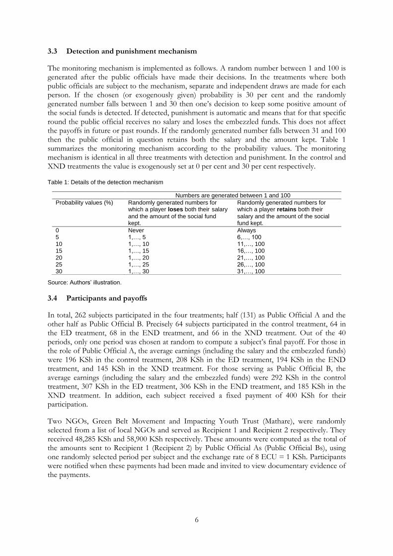
The monitoring mechanism is implemented as follows. A random number between 1 and 100 is generated after the public officials have made their decisions. In the treatments where both public officials are subject to the mechanism, separate and independent draws are made for each person. If the chosen (or exogenously given) probability is 30 per cent and the randomly generated number falls between 1 and 30 then one’s decision to keep some positive amount of the social funds is detected. If detected, punishment is automatic and means that for that specific round the public official receives no salary and loses the embezzled funds. This does not affect the payoffs in future or past rounds. If the randomly generated number falls between 31 and 100 then the public official in question retains both the salary and the amount kept. Table 1 summarizes the monitoring mechanism according to the probability values. The monitoring mechanism is identical in all three treatments with detection and punishment. In the control and XND treatments the value is exogenously set at 0 per cent and 30 per cent respectively.

Table 1: Details of the detection mechanism

Source: Authors’ illustration.

3.4 Participants and payoffs

In total, 262 subjects participated in the four treatments; half (131) as Public Official A and the other half as Public Official B. Precisely 64 subjects participated in the control treatment, 64 in the ED treatment, 68 in the END treatment, and 66 in the XND treatment. Out of the 40 periods, only one period was chosen at random to compute a subject’s final payoff. For those in the role of Public Official A, the average earnings (including the salary and the embezzled funds) were 196 KSh in the control treatment, 208 KSh in the ED treatment, 194 KSh in the END treatment, and 145 KSh in the XND treatment. For those serving as Public Official B, the average earnings (including the salary and the embezzled funds) were 292 KSh in the control treatment, 307 KSh in the ED treatment, 306 KSh in the END treatment, and 185 KSh in the XND treatment. In addition, each subject received a fixed payment of 400 KSh for their participation.

Two NGOs, Green Belt Movement and Impacting Youth Trust (Mathare), were randomly selected from a list of local NGOs and served as Recipient 1 and Recipient 2 respectively. They received 48,285 KSh and 58,900 KSh respectively. These amounts were computed as the total of the amounts sent to Recipient 1 (Recipient 2) by Public Official As (Public Official Bs), using one randomly selected period per subject and the exchange rate of 8 ECU = 1 KSh. Participants were notified when these payments had been made and invited to view documentary evidence of the payments.

Numbers are generated between 1 and 100

Probability values (%) Randomly generated numbers for which a player loses both their salary

and the amount of the social fund kept.

Randomly generated numbers for which a player retains both their

salary and the amount of the social fund kept.

0 Never Always 5 1,…, 5 6,…, 100 10 1,…, 10 11,…, 100 15 1,…, 15 16,…, 100 20 1,…, 20 21,…, 100 25 1,…, 25 26,…, 100 30 1,…, 30 31,…, 100

7

4 Results

In this paper, we are interested in the choices of Public Official A. In particular we are interested in Public Official A’s choice regarding the strength of the anti-corruption policy. We analyse only the first 20 periods, in which Public Official A receives no information about the choice made by

Public Official B.7 We start by giving some theoretical predictions before presenting subject pool

characteristics. Then, we conduct statistical tests (typically two-sided Mann-Whitney tests), before moving to regression analysis. It is important to note that statistical tests are implemented using average choices (over the 20 rounds) using each subject as an independent unit of observation while our regression analysis uses the un-averaged data.

4.1 Theoretical predictions

In this section, we discuss some theoretical predictions based on a simple model of expected utility. We focus on the END treatment, in which detection also applies to Public Official A (as shown below, the ED treatment can be seen as a special case). We assume that an official A decides to embezzle if:

(1 − 𝑝)𝑈(𝐸 + 𝑆) + 𝑝𝑈(0) > 𝑈(𝑆, 𝑣) (1)

Where 𝑝 is the probability of detection, U a utility function, 𝐸 the amount embezzled, 𝑆 the

salary received, and 𝑣 intrinsic motivation for honesty.8 Official A receives 0 (i.e. loses both

salary and amount embezzled) in case of detection and we assume 𝑈(0) = 0. As a result, an official will be corrupt if:

𝑝 < 1 −𝑈(𝑆, 𝑣)

𝑈(𝐸 + 𝑆) (2)

The decision to embezzle or not will depend on 𝑝 and 𝑣, given that 𝑆 and 𝐸 are known in our

experiment. If we assume that officials are risk-neutral and 𝑈 is additively separable, Equation 2 becomes:

𝑝 < 1 −𝑆 + 𝑣

𝐸 + 𝑆 (3)

If (1 − 𝑝)𝐸 − 𝑝𝑆 < 𝑣, indicating that intrinsic motivation is sufficiently high compared to the expected benefits from embezzlement, there will be no embezzlement.

If (1 − 𝑝)𝐸 − 𝑝𝑆 > 𝑣, meaning that intrinsic motivation is low, there will be embezzlement.

We use additional assumptions to obtain predictions from our experimental design. For example,

let’s assume 𝑣 = 0, Equation 3 boils down to:

7 From period 21 onwards, Public Official A was able to observe the amount that was transferred to Recipient 2 by Public Official B, creating endogeneity and interdependency.

8 𝑣 exists only when Public Official A is honest.

8

𝑝 < 1 −𝑆

𝐸 + 𝑆

Given that 𝐸 =1

3𝑆 in our design, Official A will be corrupt if:

𝑝 <1

4

Relaxing the risk-neutrality assumption would not change the results, except that the right-hand side of the inequality will be lower.

ED treatment

It can also be noted that the ED treatment is a particular case of the END treatment where 𝑝 = 0. In the absence of intrinsic motivation, it is always profitable to embezzle as:

𝑈(𝐸 + 𝑆) > 𝑈(𝑆)

In the presence of intrinsic motivation, we obtain the following conditions:

If 𝐸 < 𝑣, meaning that intrinsic motivation is sufficiently high, there will be no embezzlement.

If 𝐸 > 𝑣, meaning that intrinsic motivation is low, there will be embezzlement.

Generally, our expectation is that we should see a higher level of detection chosen in the ED treatment than in the END treatment, as in the END setting the level chosen also applies to Public Official A. We also expect that detection levels will be even lower when Public Official A chooses to act corruptly. Likewise, one might expect that there should be no difference in detection choices between honest and corrupt officials in the ED treatment. However, in this unconstrained setting, Public Official A’s choice of detection level reveal information about their attitude to embezzlement. Finally, in the END treatment, our simple model indicates that detection needs to be below a certain level but not necessarily equal to zero in order for a Public Official A to embezzle profitably. However, pure self-interest would lead one to expect to see a zero level of detection (or close to it) chosen when Public Official A is corrupt and higher levels chosen by honest officials. Actual choices may deviate from this prediction if Public Official A has an aversion to Public Official B’s embezzlement.

4.2 Subject pool

Table 2 presents summary statistics regarding the basic characteristics of the Public Official As in our subject pool. The participants in each treatment are on average 21 years old and in their second year of study. There are some differences across the treatments in terms of the gender composition. Gender has been found by some researchers to be important for corrupt behaviour and attitudes to corruption (Dollar et al. 2001; Frank et al. 2011; Rivas 2013). Thus, while this difference is not as pronounced between ED and END as it is with these treatments and the

9

exogenous treatments, it will be important to control for the effect of gender in our regression analysis.

The answers to the post-experiment questionnaire suggest that our subjects were well acquainted with corruption, knew the legal situation in Kenya regarding bribery, and felt that corruption by government officials is morally questionable. Of participants in the role of Public Official A, 65 per cent have paid a bribe in some circumstance. The most common bribery situations our subjects have encountered are having to pay a bribe to avoid problems with the police (17 per cent) and to get an identity document (15 per cent). Further, 69 per cent believe that some government officials are involved in corruption in their country and 27 per cent believe that all of them are engaged in such activities.

Table 2: Summary statistics of Public Official A characteristics

Variables Control ED END XND

Mean (SD) Mean (SD) Mean (SD) Mean (SD)

Age 21.56 21.09 20.97 20.67

(1.97) (2.19) (1.62) (2.06)

Gender (1 if male) 0.44 0.50 0.56 0.64

(0.50) (0.51) (0.50) (0.49)

Economics major 0.44 0.38 0.44 0.52

(0.50) (0.49) (0.50) (0.51)

Has been asked for a bribe (0 if Never) 0.59 0.66 0.62 0.73

(0.50) (0.48) (0.49) (0.45)

Owns means of transportation 0.09 0.03 0.00 0.15

(0.30) (0.18) (0.00) (0.36)

Observations 32 32 34 33

Source: Authors’ calculations based on data from the experiment.

The majority of our subjects (60 per cent) most often hear about corruption in the context of politicians and bureaucrats with the bulk of the remainder (31 per cent) most commonly being aware of corruption in terms of harassment of ordinary people for basic services. Eighty-six per cent of people understood that ‘if caught, both the bribe giver and taker are committing an illegal act’, while 8 per cent thought that only the briber taker is breaking the law. Taken together this confirms that almost all of our subjects knew that bribe-taking is legally prohibited in their country. Finally, 95 per cent of our subjects agreed that ‘it is always wrong for a government official to take a bribe.’

We begin by briefly describing and analysing the patterns in Public Official As’ corrupt behaviour before moving on to the main focus of the paper: an analysis of the choice of detection probability.

4.3 Corrupt behaviour

Public Official As faced a binary corruption choice. They could either embezzle a third of the social fund under their control or they could take nothing for themselves. The share of corrupt decisions in the control, ED, END, and XND treatments are respectively 57 per cent, 74 per

10

cent, 74 per cent, and 60 per cent.9 Two things are noteworthy. First, the lowest proportion of

corrupt decisions is to be found in our control treatment, where there was no chance of detection and punishment. The second least corrupt institutional setting was the XND treatment, where the detection probability was exogenously given. We find no significant difference between the control and XND treatments (p-value = 0.9368, two-sided Mann-Whitney). Such a result suggests that intrinsic motivation may be at play and at its strongest in the control treatment, while the disciplining effects of detection and punishment dominate in the XND treatment.

Relative to the control treatment, corruption is significantly higher in the ED treatment (at the 10 per cent level, p-value = 0.0767, two-sided Mann-Whitney) but not in the END treatment (p-value = 0.1068, two-sided Mann-Whitney). Compared to the XND treatment, we find that corruption is significantly higher both in the ED treatment (at the 5 per cent level, p-value = 0.033, two-sided Mann-Whitney) and in the END treatment (p-value = 0.046, two-sided Mann-Whitney).

The second thing to note is that the share of corrupt decisions seems to be the same, at 74 per cent, in both ED and END. We find no statistically significant difference between the two institutional frameworks (p-value = 0.8326, two-sided Mann-Whitney). Recall that the move from ED to END represents an improvement in the equality-before-the-law dimension of institutional quality holding manipulability constant. This improvement in equality does not change the corrupt behaviour of Public Official A. Since the institutional framework does not change the corrupt behaviour of Public Official A, assuming the social goal is to reduce corruption, we can evaluate the desirability of ED versus END based on the outcome with

regard to the choice of probability of detection.10

To further examine Public Official A’s decision regarding corruption, we use a random-effects Logit model. The dependent variable (Corrupt Choice) takes a value of 1 if the public official chose to embezzle some of the funds entrusted to them and 0 otherwise. The first column of Table 3 presents the results. This approach shows that there are significant differences in the propensity to be corrupt between the control treatment and both the ED and END treatments at the 5 per cent level. The result indicates that obtaining institutional power can increase the propensity to embezzle, in line with the psychological finding that power can corrupt by leading people to place greater importance on their self-interests (see e.g. DeCelles et al. 2012). In the ED treatment, Public Official A is given institutional power while being shielded from punishment. This may be taken as encouragement to be corrupt. In the END treatment, Public Official A may set the detection probability to 0 in order to shield themselves from punishment. In comparing the equality of coefficients between the XND treatment and the ED treatment, we find that the null hypothesis can be rejected at the 1 per cent level (p-value = 0.009). A similar result is found when comparing the XND and the END treatments (p-value = 0.009). No significant difference is found between the ED and the END treatment (p-value = 0.9220); or between the control and the XND treatments (p-value = 0.572). We include control variables for age, gender and having a history of experience with bribery. With the exception of age at the 10

9 In the Control, ED, END, and XND treatments, there are respectively 5, 1, 1, and 5 officials who are always honest; 18, 18, 21, and 24 officials who are occasionally corrupt; and 9, 13, 12, and 4 officials who are always corrupt.

10 Some of the 74 per cent of corrupt Public Official As may be caught in the END treatment when the probability of detection is non-zero, but this confers no social benefit as in the case of detection the funds (and salaries) are returned to the experimenter.

11

per cent level, these controls are not significant. Pursuing a major in Economics predicts corrupt behaviour significantly at the 10 per cent level (see e.g. Frank and Schulze 2000).

Table 3: Regression analysis of Public Official A’s choices

Corruption Choice (Logit)

Policy Choice—Main Effects (Tobit)

Policy Choice—Full Model (Tobit)

(1) (2) (3)

Control Baseline

ED 1.626

** Baseline Baseline

[0.808]

END 1.553** -7.955

*** -8.955

***

[0.776] [2.970] [3.255]

XND -0.457 [0.808] A's Behaviour (Corrupt=1) -0.357 -1.077 [0.890] [1.298] END # A's Behaviour (Corrupt=1) 1.362 [1.784] Age -0.238

* 0.659 0.656

[0.138] [0.785] [0.787]

Gender (1 if Male) -0.454 -3.702 -3.723 [0.562] [2.982] [2.991]

Economics as Major 1.012* -3.413 -3.428

[0.546] [3.003] [3.012]

Asked for a Bribe (0 if Never) -0.411 1.799 1.852 [0.561] [3.104] [3.114]

Owns Means of Transportation 0.258 -4.294 -4.283 [0.969] [12.443] [12.482]

Constant 5.895* 28.636 5.349

[3.102] [20.419] [17.374] Lnsig2u Constant 2.237

***

[0.218] Sigma_u Constant 11.553

*** 11.591

***

[1.182] [1.187]

Sigma_e Constant 9.851***

9.845***

[0.257] [0.256]

Observations 2620 1320 1320

Subjects 131 66 66

Note: standard errors in square brackets. * p < 0.10,

** p < 0.05,

*** p < 0.01.

Source: Authors’ illustration from own data.

4.4 Choice of detection probability

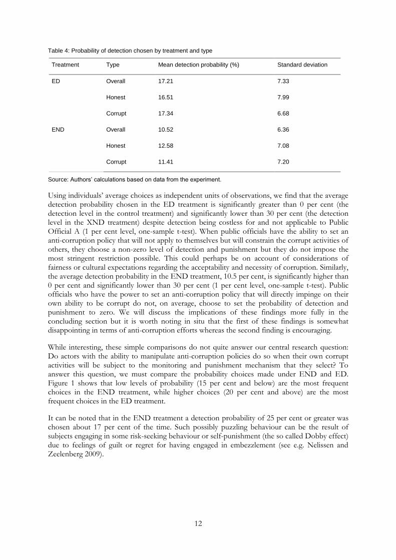
Summary statistics regarding the probability of detection and punishment chosen by Public Official A are given in Table 4. Recall that the detection rate is exogenously set at 0 per cent and 30 per cent in the control and XND treatments respectively.

12

Table 4: Probability of detection chosen by treatment and type

Treatment Type Mean detection probability (%) Standard deviation

ED Overall 17.21 7.33

Honest 16.51 7.99

Corrupt 17.34 6.68

END Overall 10.52 6.36

Honest 12.58 7.08

Corrupt 11.41 7.20

Source: Authors’ calculations based on data from the experiment.

Using individuals’ average choices as independent units of observations, we find that the average detection probability chosen in the ED treatment is significantly greater than 0 per cent (the detection level in the control treatment) and significantly lower than 30 per cent (the detection level in the XND treatment) despite detection being costless for and not applicable to Public Official A (1 per cent level, one-sample t-test). When public officials have the ability to set an anti-corruption policy that will not apply to themselves but will constrain the corrupt activities of others, they choose a non-zero level of detection and punishment but they do not impose the most stringent restriction possible. This could perhaps be on account of considerations of fairness or cultural expectations regarding the acceptability and necessity of corruption. Similarly, the average detection probability in the END treatment, 10.5 per cent, is significantly higher than 0 per cent and significantly lower than 30 per cent (1 per cent level, one-sample t-test). Public officials who have the power to set an anti-corruption policy that will directly impinge on their own ability to be corrupt do not, on average, choose to set the probability of detection and punishment to zero. We will discuss the implications of these findings more fully in the concluding section but it is worth noting in situ that the first of these findings is somewhat disappointing in terms of anti-corruption efforts whereas the second finding is encouraging.

While interesting, these simple comparisons do not quite answer our central research question: Do actors with the ability to manipulate anti-corruption policies do so when their own corrupt activities will be subject to the monitoring and punishment mechanism that they select? To answer this question, we must compare the probability choices made under END and ED. Figure 1 shows that low levels of probability (15 per cent and below) are the most frequent choices in the END treatment, while higher choices (20 per cent and above) are the most frequent choices in the ED treatment.

It can be noted that in the END treatment a detection probability of 25 per cent or greater was chosen about 17 per cent of the time. Such possibly puzzling behaviour can be the result of subjects engaging in some risk-seeking behaviour or self-punishment (the so called Dobby effect) due to feelings of guilt or regret for having engaged in embezzlement (see e.g. Nelissen and Zeelenberg 2009).

13

Figure 1: Disaggregated probability choices, by treatment

Source: Authors’ calculations based on data from the experiment.

The average chosen level of monitoring is 17.21 per cent in the ED treatment and 10.52 per cent in the END treatment. We find that the probability of detection is significantly lower in the ED treatment compared to the END treatment at the 1 per cent level (p-value = 0.000, two-sided Mann-Whitney). This fall of nearly 7 percentage points is sizeable given that the possibilities (discretely) range from 0 per cent to 30 per cent, and given the level of the averages in each treatment. Moving from END to ED would increase the strength of the anti-corruption policy by around 70 per cent (i.e. on average the chosen probability of detection increases from around 10 per cent to around 17 per cent). A similar result is found by comparing medians. The median probability choices in the ED treatment is 19.5, while the median in the END treatment is 11.62. The difference is significant at the 1 per cent level (p-value = 0.001, Median test).

We therefore conclude that there exists a statistically significant and economically meaningful distortion in anti-corruption policy-making brought about by a weak institutional framework. Specifically, it is the interaction of manipulability and equality before the law that leads to worse policy outcomes. Policy makers do not change their embezzlement behaviour when they too are subject to their policy’s provisions. Rather, they exploit the manipulability of their institutional setting to opt for a weaker policy. This institutional distortion is sizeable but not complete in that we do see a non-zero level of anti-corruption monitoring in the END treatment. This is somewhat in line with our theoretical predictions and may explain why, even in countries that are considered very corrupt, some anti-corruption efforts can be observed. But given that even low levels of monitoring have been found to be effective deterrents, this is an encouraging finding that should be of interest to all parties to anti-corruption, institutional reform, and development efforts. Furthermore, our results support the idea that shielding the decision maker from punishment or allowing them to shield themselves (at least temporarily) can provide the incentives needed for them to put into place stricter anti-corruption measures that will benefit

15.0

26.0

5.3

24.0

7.8

14.4

10.9 11.2

30.8

7.3

13.6

7.7

16.6

9.4

01

02

03

0

Fre

que

ncy

0 5 10 15 20 25 30

Treatment ED Treatment END

14

society as a whole. Recall that the decision makers in our ED and END treatments are equally likely to be corrupt. Thus, if the goal is to reduce the number of corrupt officials, allowing the

decision makers to ‘opt out’ of their own policy can be considered as a second best solution.11

An interesting analysis is to see if the choice of detection level varies according to the type (corrupt or honest) of Public Official A. In the ED treatment, corrupt Public Official As choose a detection level (17.34 per cent), which is similar to that of honest Public Official As (16.51 per cent). Likewise, in the END treatment, corrupt officials choose a similar detection level to that chosen by honest officials (11.41 per cent versus 12.58 per cent). To analyse the difference between honest and corrupt officials in the same treatment, we use Wilcoxon signed rank sum tests pairing the same individual’s average detection probability when they were corrupt and when they were honest. The differences are not statistically significant in the ED treatment (17.34 per cent when corrupt vs 16.51 per cent when honest) or in the END treatment (12.58 per cent when honest vs 11.41 per cent when corrupt).12

However, corrupt Public Official As choose a higher detection level in the ED treatment (17.34 per cent) compared to their corrupt counterparts in the END treatment (11.41 per cent) and the difference is significant at the 1 per cent level (two-sided Mann-Whitney). Thus, corrupt officials tend to distort policy to a greater extent when the policy constrains their own actions. Intentionally, distorting a policy that is in the public’s interest so that one can continue to act corruptly is in itself a corrupt act. This self-serving distortion fits the definition of state capture offered by Kaufmann and Kraay (2002). Thus, these findings can be taken as evidence of complementarity between two acts of corruption: embezzlement and institutional distortion. The observed behaviour is also in line with previous results suggesting that people who are assigned institutional powers will tend to abuse those powers for their self-interest (see e.g. DeCelles et al. 2012; Kipnis 1972; Kipnis et al. 1980).

In addition, honest Public Official As choose a higher detection level in the ED (16.51 per cent) compared to their honest counterparts in the END treatment (12.58 per cent); and the difference is significant at the 10 per cent level (p-value = 0.0614, two-sided Mann-Whitney). This shows that even policy makers who have not embezzled and therefore have nothing to fear from the detection and punishment mechanism choose a lower probability in the END treatment than in the ED treatment. This may be an unintended consequence of equality before the law in the presence of manipulable institutions. This weak institutional setting causes even honest policy makers to make socially inferior choices. We suspect that this can be explained by the fact that very few officials are fully honest (one in the ED and END treatments; amounting to about 3 per cent in each treatment), while the majority (56 per cent in the ED treatment and 62 per cent in the END treatment) are corrupt in some periods and honest in other periods. Such ‘switchers’ may feel some level of understanding and leniency towards corruption even when they are not partaking themselves in a given period.

We now proceed to a regression analysis. As the anti-corruption policy had to be chosen from a restricted range of discrete values, we employ a random-effects two-sided Tobit model for our regression analysis of Public Official A’s choice regarding said policy. The second and third columns of Table 3 present the results, which are consistent with the results of the statistical

11 Of course, many people would argue that the rule of law has intrinsic value and there are also studies that find that it is important for development outcomes. For example, Rodrik et al. (2004) conclude that the rule of law is beneficial in terms of income levels.

12 Note that with this approach, we lose observations for individuals that were always honest or always corrupt in the 20 rounds we are studying.

15

tests using averages. We find that an honest official in the END treatment chooses a lower detection probability that an honest official in the ED treatment and the difference is a statistically significant at the 1 per cent level (Column 2). In Column 2, we can also see that, overall, a corrupt official tends to choose a lower detection level compared to an honest official, though the effect is not statistically significant. Column 3 includes an interaction term between END and Public Official A’s behaviour. We can see that a corrupt official tends to choose a lower detection level compared to an honest official in the ED treatment, though the effect is not statistically significant (p-value = 0.406). Similarly, by computing the difference between average marginal effects, no significant difference is found between an honest and a corrupt official in the END treatment (p-value = 0.816). Overall, the Tobit models indicate a weaker anti-corruption policy in the END treatment. However, we find no significant difference between honest and corrupt officials in the choice of detection level either overall or within treatments.

By comparing the average marginal effects of being corrupt across treatments ED and END, we find that corrupt officials set a significantly lower detection level in the END treatment compared to corrupt officials in the ED treatment (p-value = 0.012), again suggesting complementarity between embezzlement and institutional distortion as two acts of corruption. Finally, honest officials in the END treatment choose a significantly lower detection level than honest officials in the ED treatment (p-value = 0.006). The additional control variables in the Tobit regressions are not significant at conventional levels.

5 Conclusion

This experiment analyses policy makers’ incentives to fight corruption using detection and punishment as an anti-corruption instrument. There are four treatments in which the institutional environments vary along two dimensions—equality before the law and manipulability. Equality before the law is the principle that everyone should be treated the same before the law, while manipulability refers the extent to which institutions can be manipulated by decision makers.

We find that, if given the institutional power to do so, policy makers will distort the anti-corruption instrument to reduce levels of detection when said instrument impinges, through legal equality, on their own ability to act corruptly. The magnitude of the distortion is considerable, amounting to about 70 per cent of the average detection level chosen when the detection probability does not apply to the policy maker. Even honest policy makers enact less stringent detection levels when they notionally apply to their own actions. Yet, it is important to note that, when institutions are manipulable, policy makers do not choose a zero level of detection, even when their own corrupt actions can be detected and punished. Corrupt policy makers in the END treatment choose a less stringent monitoring level than their corrupt counterparts in the ED treatment when the mechanism also threatens their own payoff. As embezzlement and weaker anti-corruption mechanisms are both contrary to the public good, this shows that corruption can beget further acts of corruption.

Standard caveats regarding the need for further and complementary evidence of course apply to our conclusions. In particular, anonymity between Public Official A and Public Official B may not hold in the field. Another important caveat, and one that is addressed in a companion paper, is that the corrupt actions of the policy maker and the institutional setting may (interactively) mitigate the effectiveness of anti-corruption policies. Even so, the implications of our findings are mostly encouraging for those invested in anti-corruption efforts in emerging and developing economies, where institutional frameworks are often viewed as weak by the standards of

16

developed countries. Encouraging the enactment of anti-corruption policies may lead to laws with some teeth, even if the law makers themselves stand to lose. An understanding of policy makers’ incentives and a willingness to let them swim through their own net (even temporarily) may serve to strengthen anti-corruption laws, possibly leading to lower levels of corruption in a society. In this regard, an interesting and potentially important avenue for further research could build on our framework and investigate whether specific ‘opt-out’ rules for policy makers have the power to lead to stronger anti-corruption efforts.

References

Abbink, K. (2004). ‘Staff Rotation as an Anti-corruption Policy: An Experimental Study’. European Journal of Political Economy, 20(4): 887–906.

Abbink, K., and M. Ellman (2010). ‘The Donor Problem: An Experimental Analysis of Beneficiary Empowerment’. Journal of Development Studies, 46(8): 1327–44.

Abbink, K., and D. Serra (2012). ‘Anticorruption Policies: Lessons from the Lab’. Research in Experimental Economics, 15: 77–115.

Abbink, K., B. Irlenbusch, and E. Renner (2002). ‘An Experimental Bribery Game’. Journal of Law, Economics, and Organization, 18(2): 428–54.

Abbink, K., U. Dasgupta, L. Gangadharan, and T. Jain (2014). ‘Letting the Briber Go Free: An Experiment on Mitigating Harassment Bribes’. Journal of Public Economics, 111: 17–28.

Azfar, O., and W.R. Nelson Jr (2007). ‘Transparency, Wages, and the Separation of Powers: An Experimental Analysis of Corruption’. Public Choice, 130(3–4): 471–93.

Barr, A., M. Lindelow, and P. Serneels (2009). ‘Corruption in Public Service Delivery: An Experimental Analysis’. Journal of Economic Behavior & Organization, 72(1): 225–39.

Berninghaus, S.K., S. Haller, T. Krüger, T. Neumann, S. Schosser, and B. Vogt (2013). ‘Risk Attitude, Beliefs, and Information in a Corruption Game—An Experimental Analysis’. Journal of Economic Psychology, 34: 46–60.

DeCelles, K.A., D.S. DeRue, J.D. Margolis, and T.L. Ceranic (2012). ‘Does Power Corrupt or Enable? When and Why Power Facilitates Self-interested Behavior’. Journal of Applied Psychology, 97(3): 681–89.

Dollar, D., R. Fisman, and R. Gatti (2001). ‘Are Women Really the “Fairer” Sex? Corruption and Women in Government’. Journal of Economic Behavior & Organization, 46(4): 423–29.

Engel, C., S.J. Goerg, and G. Yu (2013). ‘Symmetric vs. Asymmetric Punishment Regimes for Bribery’. Max Planck Institute Collective Goods Preprint (2012/1). Bonn: Max Planck Institute.

Frank, B., J.G. Lambsdorff, and F. Boehm (2011). ‘Gender and Corruption: Lessons from Laboratory Corruption Experiments’. European Journal of Development Research, 23(1): 59–71.

Frank, B., and G.G. Schulze (2000). ‘Does Economics Make Citizens Corrupt?’. Journal of Economic Behavior & Organization, 43(1): 101–13.

Fritzen, S. (2005). ‘Beyond “Political Will”: How Institutional Context Shapes the implementation of Anti-corruption Policies’. Policy and Society, 24(3): 79–96.

17

Hanna, R., S. Bishop, S. Nadel, G. Scheffler, and K. Durlacher (2011). The Effectiveness of Anti-corruption Policy. EPPI Centre Report 1909. London: EPPI Centre, University of London.

Heeks, R., and H. Mathisen (2012). ‘Understanding Success and Failure of Anti-corruption Initiatives’. Crime, Law and Social Change, 58(5): 533–49.

Kaufmann, D., and A. Kraay (2002). ‘Growth without Governance’. World Bank Policy Research Working Paper 2928. Washington, DC: World Bank.

Kipnis, D. (1972). ‘Does Power Corrupt?’. Journal of Personality and Social Psychology, 24(1): 33–41.

Kipnis, D., S.M. Schmidt, and I. Wilkinson (1980). ‘Intra-organizational Influence Tactics: Explorations in Getting One’s Way’. Journal of Applied Psychology, 64(4): 440–52.

Levitsky, S., and M.V. Murillo (2009). ‘Variation in Institutional Strength’. Annual Review of Political Science, 12: 115–33.

Makowsky, M.D., and S. Wang (2015). ‘Embezzlement, Whistleblowing, and Organizational Structure’. GMU Working Paper in Economics 15–59. Fairfax, VA: George Mason University.

Mungiu-Pippidi, A. (2006). ‘Corruption: Diagnosis and Treatment’. Journal of Democracy, 17(3): 86–99.

Mutebi, A.M. (2008). ‘Explaining the Failure of Thailand’s Anti‐corruption Regime’. Development and Change, 39(1): 147–71.

Nelissen, R., and M. Zeelenberg (2009). ‘When Guilt Evokes Self-punishment: Evidence for the Existence of a Dobby Effect’. Emotion, 9(1): 118–22.

North, D.C., J.J. Wallis, and B.R. Weingast (2009). Violence and Social Orders: A Conceptual Framework for Interpreting Recorded Human History. Cambridge: Cambridge University Press.

Olken, B.A. (2007). ‘Monitoring Corruption: Evidence from a Field Experiment in Indonesia’. Journal of Political Economy, 115(2).

Rivas, M.F. (2013). ‘An Experiment on Corruption and Gender’. Bulletin of Economic Research, 65(1): 10–42.

Robinson, J.A., and D. Acemoglu (2008). ‘Persistence of Power, Elites and Institutions’. American Economic Review, 98(1): 267–293.

Rocha Menocal, A., N. Taxell, J.S. Johnsøn, M. Schmaljohann, A.G. Montero, F. De Simone et al. (2015). Why Corruption Matters: Understanding Causes, Effects and How to Address Them. DFID Evidence Paper. London: Department for International Development.

Rodrik, D., A. Subramanian, and F. Trebbi (2004). ‘Institutions Rule: The Primacy of Institutions over Geography and Integration in Economic Development’. Journal of Economic Growth 9(2): 131–65.

Schickora, J. (2011). ‘Bringing the Four-eye Principle to the Lab’. Munich discussion paper 2011–13. Department of Economics, University of Munich.

Schulze, G.G., and B. Frank (2003). ‘Deterrence versus Intrinsic Motivation: Experimental Evidence on the Determinants of Corruptibility’. Economics of Governance, 4(2): 143–60.

Serra, D. (2012). ‘Combining Top-down and Bottom-up Accountability: Evidence from a Bribery Experiment’. Journal of Law, Economics, and Organization, 28(3): 569–87.