Why don’t all Exporters Benefit from Free Trade Agreements?Estimating Utilization Costs ∗

Alfie Ulloa † and Rodrigo Wagner-Brizzi ‡ §

version as of May 1, 2013 [1st version: May 02, 2012]

Abstract

Free Trade Agreements (FTA) attract significant interest, but after these treaties are signed notall exporters use them. We provide a model of heterogeneous utilization, also developing a novelmethod to estimate treaty-utilization costs. We later apply the model to estimate the evolutionutilization costs for the FTA between the US and a small open economy, Chile. Consistent withother studies, we find that utilization is indeed partial (on average 67% on the first year of thetreaty, with 10 percentage points more at the third year). This made tariff revenues to the US10% higher than expected with full utilization. Our simple structural model identifies costs byexploiting the indifference condition for the smallest firm that uses the treaty. Empirically wefind that estimated costs were very heterogeneous across products. For almost half the productsthe cost was not binding for any exporter. However, when the FTA started, the 75-th percentileof utilization cost was around US$3,000, requiring shipments above $80,000 to justify usingthe treaty. These costs decreased by 60-80% in the following years, consistent with models oflearning about treaty use. As remarked in our model, small exporters that do not use the tradeagreement could even suffer when large firms have the option of using the treaty, since the latterincrease exports and may push up factor prices for the industry.JEL classification: F1Key words: Heterogeneous effects of trade agreements, Small and Medium Enterprises (SME),Policy implementation.

∗Authors acknowledge the valuable conversations with Andres Rodriguez-Clare, Carolyn Roberts, Ricardo Haus-mann and Sebastian Bustos; as well as seminar participants at Tufts, IADB and IIOC in Boston. Patrick O’Hallaranprovided superb research assistance while Erick Feijoo helped with data support at IADB. A portion of this researchwas supported by grant by the Inter-American Development Bank and benefited from data sharing by Chilean Cus-toms (Servicio Nacional de Aduanas) through the Chilean Ministry of Finance. Usual disclaimers apply

†University of Chile, Law School and ZBU‡Assistant Professor at Tufts University, Economics Dept. ; Associate at Center for International Development

(Harvard University) ; Affiliate to the Entrepreneurship & Firm Growth (SME) research group at Innovations forPoverty Action (IPA).§Corresponding author: Rodrigo.Wagner@Tufts.edu - 8 Upper Campus Road, Medford MA. 02155. USA.

1

1 Introduction

As of January 2012, the World Trade Organization records 251 active Regional Trade Agreements(RTA) between two countries or blocks of countries, the highest number in modern history. Theentry into these agreements have been particularly exciting for exporters in small economies, espe-cially when they start an agreement with a large and developed area, like the US or the EU. In fact,many governments push the approval of these agreements selling it as a substantial developmentalmilestone that could help firms that currently export to these large markets, as well as to the manyfirms that will start doing it in the future. 1 In fact many papers analyze the benefits and costsof these trade agreements, but the overwhelming majority of these analyses assume that tradeagreements are used by all exporters. In this paper we try to unpack utilization rates, which is thefraction export value that takes advantage of the trade agreement and pays lower tariffs. Thus,we center our work in a process that starts “the day after” the treaty begins, where governmentauthorities usually like firms to take full benefit of the TA. 2

In this paper we first explore the implications of heterogeneous utilization of a treaty with a simplemodel. The model argues that a fixed cost of utilization can rationalize partial utilization within thesame industry. Furthermore, the model shows that these costs could even make smaller exportersworse off after the trade agreement, since these smaller firms will not use it, while larger firmswould take advantage of it this pushing up factor prices. After introducing the relevance of theseutilization costs, we offer a novel and simple structural model to estimate treaty utilization costs,a methodology that we later apply to understand the early years of a trade treaty between Chileand the US. Our empirical findings start first as basic aggregate stylized facts that motivate ourmodel, while later we focus on identifying the fixed costs

First, utilization is large - especially when compared to ASEAN countries described in the literature- but it is far from complete. The average utilization rate of a product in the FTA began at aroundtwo thirds at the moment the treaty started, when weighting all products equally, irrespective oftheir trade volume. In the following two or three years of the treaty, the utilization rate reacheda “plateau” of around 80-85%. In short, for the average product that arrives to US Customs and

1Consider for example the following statement by the Chilean president during a speech analogous to the “Stateof The Union”. “Es el Chile que logró un Tratado de Libre Comercio con la principal potencia del mundo, los EstadosUnidos de América, el cual está en vías de ser ratificado por ambos Congresos. Estos acuerdos, que serán seguidospor otros, son una sólida garantía para nuestro desarrollo. Las oportunidades que se abren son enormes. Cuando laeconomía mundial entre en un ciclo ascendente estaremos preparados para no dejar escapar estas nuevas oportunidades” Ricardo Lagos, May 21st 2003; months before the beginning of the US-Chile treaty in Jan 1 2004.

2In the very recent case of Colombia, for example, after signing the FTA treaty with the US they nominated aPresidential Delegate for FTA utilization. In the case of Chile, 8 years after the treaty with the US started, boththe President and the Association of Entrepreneurs have expressed concerns that the FTA with the US has not beenused as much as they would like.The Recently Formed Association of Chilean Entrepreneurs met the Chilean President and gave him a list of

ten priorities for them. The ninth was about the “visibility” of FTA for entrepreneurs “9. A pesar de los tratadoscomerciales firmados y de abrir las fronteras comerciales, las tasas de ocupación de las cuotas otorgadas por diversospaíses a productos chilenos, son todavía bajas. Por eso, Asech promueve la creación de plataformas de trabajo enChile y el extranjero, que hagan visibles a los emprendedores nacionales las oportunidades que ofrecen los Tratadosde Libre Comercio (TLC).”

2

after various years, one in seven products still do not use the treaty, meaning that they are payinghigher tariffs to the US as if they treaty did not exist. When we weigh the use by the volume ofexports we found that in the first year of the treaty, Chilean exporters did not use around 10% ofthe tariff benefits. This figure of “surprising” government revenue for the US decreased to 3% andthen took off during the financial crisis; reaching again around 10% in 2010.

Second, as expected, the higher the tariff preferences the higher the utilization rate. When lookingat within product variation, a one percentage point gap between the lower FTA tariff and thestandard “Most Favored Nation”(MFN) rate is associated with slightly more than one percentagepoint of additional utilization. It is interesting, though, that we do not find significant effects forhaving small non-zero tariff preferences, like 0.1 percentage points preferences. This is consistentwith a model where there is a fixed cost of utilization and, without enough benefits, firms stillprefer to use the standard MFN regime and avoid the fixed cost. 3

After these two sanity checks: that utilization is partial and that tariffs matter, we develop a simplemethodology to calculate product-specific fixed costs of utilization using data usually available forgovernments, so the method could be of independent interest for other researchers. We focus on themarginal firm that is indifferent between using the treaty or not. Using the empirical distributionof export volume by firm in a product, as well as the empirical utilization rate u , we calculatefixed costs as the amount that rationalizes not taking the tariff benefits. The estimated cost isvery heterogeneous across products. For the 75-th percentile of our sample it was around threethousand dollars, with a sharp decline of more than 60-80% in the following two years. This declineis consistent with models of learning in early stages of a treaty; although it is less clear whetherthis knowledge is internal or external to firms.

There are more than thousand papers about free trade agreements and other forms of regional eco-nomic integration, with various reviews including the handbook chapter by Baldwin and Venables(1995) and the more recent survey by Freund and Ornelas (2010). Our work, however, adds to amuch less advanced literature that focuses on how firms utilize these treaties. Various strategieshave been used to explore them.

The least data intensive strategy to understand utilization looks at aggregate trade flows, indirectly3To explore some plausible determinants of these fixed costs, like Anson, Cadot, Estevadeordal, Melo, Suwa-

Eisenmann, and Tumurchudur (2005) and Carrere and de Melo (2004), we tried to see whether tougher rules oforigin are related to lower utilization rates. Nonetheless, we found the opposite, that products with tougher rulesof origin are consistently those which use the treaty the most; and since there is no plausible reason for a positivecausal effect of restrictions on utilization, we interpret this fact as evidence that in the negotiation of the FTA, Rulesof Origin are imposed as a burden to sectors that may appear ex ante as more competitive.These tougher rules oforigin could be interpreted as a way to delay the effect of a free trade agreement on domestic firms that compete withnew exporters. Maybe as a de facto way to implement delayed tariff reduction as suggested by models like Maggiand Rodríguez-Clare (2007) , although in our data we do not find relevant time variation within product in the RoOrequirements. That is why we focus on estimating product level barriers and explore their evolution over time, astariffs change.Rather than using a single synthetic index for ROO restrictiveness, as Anson, Cadot, Estevadeordal, Melo, Suwa-

Eisenmann, and Tumurchudur (2005) do, Carrere and de Melo (2004) include various types of rules and explore howthese impact the Mexico-NAFTA trade. We follow them including various types of indicators for rules of origin.

3

inferring magnitudes of interest, like fixed costs of utilization or the impediments generated by rulesof origin. Hayakawa (2011) calculated reduced-form estimates of the fixed cost of using a FTA usinga standard gravity equation with aggregate data, and then adding as explanatory variables boththe tariff and the interaction between tariffs and FTA to exploit a discontinuity. Their estimate forthe average fixed cost of using trade agreement in the world is equivalent to a 3% tariff. This wouldbe a very large cost, since many times the average tariff reductions in modern FTA are not farfrom that level. Anson, Cadot, Estevadeordal, Melo, Suwa-Eisenmann, and Tumurchudur (2005)also use aggregate data in a gravity regression, but now attempting to disentangle the effect oftariffs and rules of origin (RoO), finding some support for the idea that some RoO may undo thetariff benefits.4 In any case, the main complication of using only aggregate data is that it mixestogether the selection effects with the causal effects of FTAs on firm behavior. Our work, awareof data limitations, tries to exploit the information in the utilization shares and the distributions,to estimate fixed costs, in the spirit of what has been done in the industrial organization literature(e.g. Olley and Pakes, 1996).

A second research strategy - more intensive in micro data collection - asks firms whether they usetreaties or not. In two companion papers Takahashi and Urata (2008, 2009)use a survey of sixteenhundred Japanese firms made in 2008 (with 15% response rate), where they find that 32.9% ofJapanese exporters to Mexico used the treaty, noting that this is almost twice as much as thereported use in 2006, two years before. This increased utilization might be consistent with theutilization increasing over time as in learning models. 5 Trying to unpack the heterogeneity acrossfirms, Hayakawa, Hiratsuka, Shiino, and Sukegawa (2009) use firm level data but restrict theiranalysis to a survey of a few hundred Japanese affiliates in the ASEAN region, finding that thescale of the firm is an important determinant of the likelihood of utilizing the FTA, even amongthis sample of multinationals. Nonetheless, they have serious limitations dealing with heterogeneityacross products. Given their data is by firm, when they analyze destinations, they do not workwith product specific tariffs but, instead, they rank countries by their average tariff rate (e.g. Chinahaving higher tariffs than Japan, and so on). This is important since many the utilization costs -paperwork, certification, etc - are product specific rather than firm specific.

Our empirical approach is different from these exercises for Japanese firms in a number of ways.4Anson, Cadot, Estevadeordal, Melo, Suwa-Eisenmann, and Tumurchudur (2005) focus on how Rules of Origin

(ROO) constrain exports within a FTA zone. They argue that in many cases ROO can partially or totally unduethe tariff preference. Their central point is that in the negotiation process of a North-South FTA, the North imposesROO even up to the point of leaving the South-country exporters indifferent between using or not using the treaty.First they run a global gravity regression adding coefficients for Trade Agreements, and also adding an index of ROOthat goes from 1 to 7. The negative coefficient on ROO supports the idea that ROOs put sand on the wheels of aFree Trade Area. Then the authors use product level data for Mexican Exports to the US before and after NAFTAto study the specific case. Their empirical strategy assumes that products with utilization rates of the treaty strictlybetween zero and one (i.e. partial use of the treaty,0 < uit < 1) are the products for which firms are indifferentbetween using and not using the treaty. The authors acknowledge this is not the only possible interpretation. In fact,the partial use when data is aggregated at the product level may reflect that some firms are using the FTA whilesome others are not; which would be the case when firms are heterogeneous in either the costs or the benefits of use,as shown theoretically by Ju and Krishna (2002) and Demidova and Krishna (2007). In section

5They also find that 23.7% Japanese exporters to Chile use the FTA.

4

The first reason is because we are arguably working with the population of all exports from Chileto the US, rather than a survey . Second, we have product specific information, indicating theuse of products in a particular product line. This is very important since a lot of exporting isdone by multi- product firms and also because the tariff benefits are defined with fine granularity.One limitation, though, is that we do not know exactly which firms used the FTA, because that isusually confidential data of the importer country.6 Nonetheless, using micro data from the exportercountry and a few assumptions we could get an estimate of the marginal user of the treaty.

We have to acknowledge one paper that has simultaneously utilized micro-data for a population ofexporters and products. Kohpaiboon (2008) explore FTA use by Thai manufacturers, benefitingfrom the fact that exporters in Thailand must apply to Thai customs to get a certificate of origin(instead of a self-certification plus a submission at the importer’s customs, which is the case forUS imports and for many other modern treaties). They find that Rules of Origin are equivalentto an additional 2% tariff in their effect on utilization, but uses standard regressions rather thanlooking at the marginal user as we are doing. While our paper has micro-data on firms but not onutilization, we believe our method could be more broadly applied to many real policy evaluation ofFTA implementation, because the data observed in Thailand will unlikely be available to researchersin most other countries.

A final relevant difference of our paper is our setting. Most of the papers analyzing utilizationof FTA are disproportionally looking at economies producing manufacturing goods, usually withthe value chain split across nearby countries (e.g. ASEAN, Mexico-US maquila)7 In contrast, dueto distance from main markets and production mix, in our setting we need to worry less aboutexporting after intermediate processing of imported inputs. Moreover, unlike in many ASEANeconomies and Mexico in NAFTA, a large fraction of Chilean goods are not manufacturing, butproducts which inputs are more likely to be sourced domestically (think of Copper, Pulp paper andWines). Maybe for these reasons we fail to find negative correlation between rules of origin andvolumes.

After clarifying the contributions and limitations of our work, we draw a map for the rest of thepaper. Section 2 describes a simple framework of treaty heterogeneous utilization. Section 3 takes

6Papers analyzing utilization rates by product, likeJames (2007), usually go to the United States InternationalTrade Commission database and download utilization rates, calculated as the share of value that enters US docksclaiming the FTA. The numerator of that share is straightforward, since it is just the amount claimed. The key forthe interpretation of the results is what you put in the denominator of that share, because of at least two importantconsiderations. First, a significant fraction of products have free MFN tariff rate even before the treaty start, so wewould never expect any use and of course it was never meant to be an “impact” of the treaty. We take care of this issueby simply excluding these products from the analysis. Second, the treaties usually do not involve immediate tariffreduction, but sequential reductions depending on their staging category. For products where staging has not yetcreated a wedge between the MFn and the FTA tariffs, then in practice the treaty has not began for those products.We also exclude these groups from most of our analysis. As a result, we focus on products that are meant to be usedin a FTA, and any difference in at least some use could be attributed to either compliance costs (including but notonly those resulting from tough Rules of origin) and informational frictions.

7For example: Thailand in the ASEAN context (Kohpaiboon, 2008); Mexico (Anson, Cadot, Estevadeordal,Melo, Suwa-Eisenmann, and Tumurchudur, 2005; Carrere and de Melo, 2004 ); and Japanese affiliates in ASEAN(Hayakawa, Hiratsuka, Shiino, and Sukegawa, 2009).

5

the above mentioned model and shows the conditions under which one can estimate the fixed uti-lization costs. Section 4 describes our data and the treaty, outlining basic stylized facts. Followingup, section 5 uses regressions to explore utilization dynamics and the role of tariff preferences.Section 6 estimates our simple structural model to back out fixed utilization costs by product overtime using the Chile-US FTA. Section 7 we concludes with some remarks.

2 A framework of partial treaty utilization

This section describes a model where heterogeneous exporters endogenously decide whether to use afree trade agreement or not, which we denote as the binary decision use. If they use the agreementthey have to pay a fixed cost f and get tariff free access, while if they do not use the agreement,they save on f but have to pay tariff τ . The industry has a single non-tradable input called L,which should not be interpreted as standard labor but something more industry specific that has aendogenous cost w per unit. There is only a single foreign market (the US) and, for simplicity, thereare no domestic sales because the country does not consume what it produces. We also assumeall firms export. We could add the prerequisite decisions to open a firm and to start exportingnon-zero quantities, like Melitz (2003) does, but this would add more complexity to the derivationswithout an important payoff in terms of additional economic intuition, so we abstract from thesefeatures.

A firm of type j follows a production technology with decreasing returns to scale: ϕjlα, whereϕi is the heterogeneous productivity, l is the endogenous input choice of the firm and α ∈ (0, 1)determines the returns to scale. Unlike in benchmark models of heterogeneous firms (i.e. Melitz,2003) we assume that the limits to firm size come from production that is hard to scale, rather thanfrom demand. Nonetheless that assumption is not essential and our argument could be adapted formodels with constant returns to scale and CES demand. We assume the industry is in a small openeconomy that takes as given the destination market’s price p of the good. A firm maximizing oper-ational profits would have an input demand of l (ϕ) = (αpϕ/w)1/(1−α), with export values x (ϕ) =pϕ1/(1−α) [αp/w]α/(1−α) and the operational profit function is8 [1− α] [α/w]α/(1−α) [pϕ]α/(1−α). Ifwe further assume, without losing generality, that the tariff-free FOB price is p = 1, while the FOBprice with tariff is p = 1/ (1 + τ), we get the profit function of using the treaty (use = 1) and not

8Replacing the input demand we get pϕ [αpϕ/w]α/(1−α) − w [αpϕ/w]1/(1−α); which could be simplified as

[pϕ]1+ α1−α

[ 1w

]α/(1−α)αα/(1−α) − w1− 1

1−α [pϕ]1/(1−α) α1/(1−α)

=[ 1w

]α/(1−α)[pϕ]

11−α

[αα/(1−α) − α1/(1−α)][ 1

w

]α/(1−α)[pϕ]

11−α

{α

α1−α [1− α]

}

6

using the treaty (use = 0), namely:

π (ϕ|use = 1) = [ϕ]α/(1−α) [1− α][αw

]α/(1−α) −f

π (ϕ|use = 0) =[ϕ

1+τ

]α/(1−α)[1− α]

[αw

]α/(1−α)

Heterogeneous productivity distributes G (ϕ), with ϕ ∈(ϕ, ϕ̄

). Although we do not need it for our

qualitative results, to simplify we will assume the distribution is Pareto with ϕ = 1 and ϕ̄ = ∞;such that Pr (ϕ̃ > ϕ) = ϕ−γ ; so cumulative density G (ϕ) = 1− ϕ−γ and density g (ϕ) = γϕ−γ−1;with a technical restriction on the relation between γ and α so the mass of production does not goto infinity as ϕ goes to infinity. Namely η ≡ γ − 1

1−α has to be positive.

The model has two aggregate endogenous variables: the wage rate w and the productivity of thecutoff treaty userϕ̂. To solve for these two unknowns the model has two equilibrium conditions: (i)the indifference condition for the marginal treaty user and the (ii) equilibrium in the input market.

The cutoff ϕ̂defining the marginal user could be found graphically when the two profit functionsintersect, as depicted in Figure 1. Algebraically, ϕ̂ solves π (ϕ̂|use = 0) = π (ϕ̂|use = 1); whichimplies

ϕ̂ = w

f

αα/(1−α) [1− α][1−

(1

1+τ

)α/(1−α)]

(1−α)/α

(1)

; and as expected, the cutoff ϕ̂ increases with conditions that discourage the marginal firm to usethe treaty, like the fixed cost f and the wage w , while it decreases when it becomes more profitableto use it, namely when tariffs for non users τ are larger. Eq. 1 shows a monotonically increasingrelation between the two endogenous variables w and ϕ̂.

7

π

ϕ

π(ϕ|use = 0)

−fA

π(ϕ|use = 1)

use FTAnon users

ϕ̂

Figure 1. Cutoff productivity for using the Free Trade Agreement when α = 0.5

Instead, the equilibrium in the non-traded input market would create a downward sloping relationbetween the two endogenous variables w and ϕ̂. This equilibrium requires input supply LS to matchthe aggregate demand for inputs LD. It is now usual in the literature on heterogeneous exportersto focus on the case when input supply is inelastic, so L′S (w) = 0. Following this tradition we willnot model explicitly input supply, but we would allow for any non-negative input-price elasticityL′S (w) ≥ 0. To simplify we assume fixed costs are paid out of profits, so f does not enter directly

into the input market clearing condition. Aggregate input demand LD is computed integratingindividual input demands over non-users and users of the treaty LD =

´ ϕ̂1 l (ϕ|use = 0) dG (ϕ) +´∞

ϕ̂ l (ϕ|use = 1) dG (ϕ); which after solving the integration becomes:

LD = 1λ (w)

[(1− 1

τ̃

)ϕ̂−η + 1

τ̃

]

; where η = γ−1/ (1− α) > 0 ; 1/τ̃ ≡ [1/(1 + τ)]1

1−α with 1/τ̃∈(0, 1) and 1/λ (w) ≡ γη

[αw

] 11−α with

λ (w) > 0 . Input market equilibrium needs LS = LD, which yields

LSλ (w) = 1ϕ̂η

[1− 1

τ̃

]+ 1τ̃

(2)

; which, as anticipated before, is a decreasing relation between w and ϕ̂ , while it does not dependdirectly on the fixed utilization costs f .

Since both conditions in Eq. 1 and Eq. 2 have monotonic slopes, there will be a unique equilibrium

8

for the two endogenous variables, as depicted in Figure 2. This equilibrium would exist as long as9 the fixed cost f should be large enough so at least some firms are left without utilization despitethe benefits of not paying a tariff.

w

ϕ̂

LDemand(w, ϕ̂) = L̄Supply

πuse(ϕ̂, w) = πnotuse(ϕ̂, w)

ϕ̂∗1

w∗

Figure 2. Endogenous determination of wage w and marginal user of the treaty ϕ̂ using both theindifference condition for the marginal user of the treaty and the labor market clearing condition .

Note that the positive sloped relationship defined by the indifference shifts to the right when fixedutilization costs f increases (see Eq 1), while the downward sloped Labor Market does not dependon f (see Eq 2). We can understand a Free Trade Agreement as a decrease in f from infinity (sobefore the treaty no firm could use the treaty!) to a finite value where some firms starts using it.This would make then the price of inputs w increase as the πuse = πnon−use curve moves to theleft, leaving non users worse off than without the treaty, since they have to pay higher wages andthey can’t access the treaty. 10 Formally, the slope of the input market equilibrium line in Figure2 is obtained by implicitly differentiating Eq 2, which yields.

∂w

∂ϕ̂

∣∣∣∣LS=LD

=−(1− 1

τ̃

)ϕ̂−η−1

L′S (w)λ (w) + LS (w)λ′ (w) ≤ 0

; this implies that there is an exception to our point that non-users lose from the treaty; becausewhen the non-traded input supply LS is perfectly elastic to w, so is L′S (w); then clearly the inputmarket equilibrium has a flat wage. Thus, our main proposition goes as follows.

Proposition 1. Low productivity firms that in equilibrium would export but not use the treaty9We need ϕ̂ > 1 and w > 0 as required by the model. To get ϕ̂ > 1 using the condition for the marginal user Eq

1 we need[fA/

[αα/(1−α) [1− α]

[1−

(1

1+τ

)α/(1−α)]]](1−α)/α

> 1/w.10We have to highlight that in our simplified model there is no exit margin but it could be easily added. Nonetheless,

this would not change our channel of interest of winners and losers from a free trade agreement with some utilizationcosts.

9

(meaning ϕ < ϕ̂ (fA, τ) ) , would decrease their profits when the treaty starts, since inputprices w would increase without any positive effect on profits. This happens except wheninput supply is perfectly elastic (meaning L′S (w) =∞), in which case non-users neither gainnor lose from having the treaty.

In short, these losses for non-users could be more important when inputs are highly non-tradableand in short supply within the country, while less relevant if the supply of inputs reacts to scarcity.As mentioned in the introduction, however, our goal in this paper will not be to test this proposition,which we leave for further research, but to use the framework as a lens to do econometric analysisand measure the evolution of fixed costs. Having developed the framework, the next section tellshow we could build a simple structural model.

3 A simple structural model of treaty utilization

Using our model we can now define the utilization rate, u, following closely the method of calculationuse by customs in importing countries (i.e. US Customs in our case). Thus u is the share of theFOB value exported using the treaty over FOB. Meaning

u =´∞ϕ̂ x (ϕ|use = 1) dG (ϕ)´ ϕ̂

ϕ x (ϕ|use = 0) dG (ϕ) +´∞ϕ x (ϕ|use = 1) dG (ϕ)

10

; where as defined previously x (ϕ) is the FOB value exported by each firm. After solving theintegral and using the simplifications discussed before, we can express utilization rate as:11

u = 11 + 1

τ̃ [ϕ̂η − 1](3)

so u ∈ (0, 1] because when ϕ̂ = ϕ = 1 , then utilization if complete, u = 1; while when ϕ̂ → ∞ ,like before the treaty is implemented, we have u → 0. As expected ∂u/∂ϕ̂ < 0 ; so the larger thecutoff the smaller the utilization rate. Note that for the special case in which input supply LS isperfectly elastic, then we know from Eq 1 that ∂ϕ̂/∂τ̃ < 0 ; and applying this in Eq3 we can showthat utilization raises with the tariff, meaning ∂u/∂τ > 0.

Although these utilization rates have been the dominant metric to understand the success of thetreaty, the evolution of u within a product across time can give a misleading picture on whether itis getting easier or more difficult to use the treaty. Imagine for example a case where three firmsexport the product but only two of them use the treaty. If we also imagine that over time the twofirms using it start exporting disproportionally more value, then the measured utilization rate ofthe product (ui,t) would increase, because it is a value weighted statistic. Moreover, an increasingutilization rate is consistent with the worsening of utilization costs. Thus, to have a better viewof the barriers to use trade agreements we would like to know also whether the conditions for themarginal firm using the treaty are easing over time or not, meaning the evolution of the fixed costfA.

To estimate this we would like to know exactly who is using it and who is not. But for almost allcountries, utilization measures are available only as aggregates at the product-level on importers’Customs, and it is not separated firm by firm.12 But with this model in mind, and some assump-tions, we can use data usually available to governments to estimate f . We just need importer

11

u =γ[αw

]α/(1−α) ´∞ϕ̂ϕ−η−1dϕ

γ[

11+τ

] 11−α

[αw

]α/(1−α) ´ ϕ̂1 ϕ−η−1dϕ+ γ

[αw

]α/(1−α) ´∞ϕ̂ϕ−η−1dϕ

u =´∞ϕ̂ϕ−η−1dϕ[

11+τ

] 11−α´ ϕ̂

1 ϕ−η−1dϕ+´∞ϕ̂ϕ−η−1dϕ

u =

[ϕ−η

]∣∣∞ϕ̂[

11+τ

] 11−α [ϕ−η]|ϕ̂1 + [ϕ−η]|∞ϕ̂

u =1−η

[−ϕ̂−η

][1

1+τ

] 11−α 1

−η [ϕ̂−η − 1] + 1−η [−ϕ̂−η]

u =[ϕ̂−η

]1τ̃

[1− ϕ̂−η] + [ϕ̂−η]

u = 11τ̃

[1− ϕ̂−η] ϕ̂η + 112As mentioned, one of the few exceptions is Thailand Kohpaiboon (2008); but their dataset is unlikely to be

available in other countries, especially because many FTAs are moving towards self certification.

11

(say US Customs) data on aggregate utilization rates u at the product level, and combine it withnational data on the export size distribution of firms in a product, which is usually a databaseproduced by Customs. 13

From such a database of exporters sizes, one calculates the cumulative density of export valuesG̃ (x), which gives the probability that a dollar exported by the country comes from a firm of sizesmaller or equal to x, where size is measured only in terms of dollars and not domestic sales, sincewe assume the problems were separable for the firm. This cumulative export density G̃ (x) hasG̃ (x̄) = 1 and G̃ (x) = 0; where for notational simplicity G̃ (x) ≡ G̃

(x(ϕ))

and an analogousexpression for ϕ̄. Most important for our purposes, the cumulative export density G̃ (x̂)for themarginal user of the treaty ϕ̂ equals the complement of the utilization rates. Meaning

G̃ (x̂) = 1− u (4)

; as shown in Figure .

x Exporter size

G̃(x) Cumul export size density1

1− u

x̂

Then f = x̂ ·∆τ

utilization u

Figure 3. Solving for the marginal user x̂ knowing the utilization rate u and the cumulative exportdensity function G̃ (x). Once x̂ is identified one calculates the utilization cost f = x̂ ·∆τ

With this at hand we need three assumptions to identify the fixed cost f from the data:14

Assumption 1. At the margin of utilization, ϕ̂, the change in profits is small enough so we canapply the Envelope theorem, so ∂π (ϕ) /∂τ = x (ϕ)

13This would make the method below useful for almost any government, including places like Peru or Colombiathat recently signed a FTA with the US.

14As the rest of the literature we assume f is constant across firms. This assumption is not essential for thecalculation, since we always can interpret the measured f , called f̂ , as just a local fixed cost rather than the constantfixed cost, but this assumption clarifies our interpretation. Also, we are assuming that the cost is per firm eachyear. In the appendix we discuss the potential biases when reality deviates from this assumption. Extending this todynamic settings where expectations about future exports matter will be the subject of future research.

12

Assumption 2. Pecking order use. All firms above the cutoff use the treaty while firms below thecutoff do not use the treaty.

Assumption 1 allows us to use the Envelope theorem and, at the margin, keep the optimizedexported quantities constant while just changing the price received due to the changes in tariffs.This step is not essential, since we could use the full model in Section 3 to predict how quantitychanges when the after-tariff price changes, but the assumption greatly simplifies the mappingfrom observed export volumes to fixed costs. In particular, when using the envelope theorem ourcalculation does not need as input any additional parameter (like α , γ or even w). This allows us tomeasure f just as a function of u, G̃ (x) and tariffsτ , all these quantities are observed directly fromthe data. Importantly, the fact that we consider the change in quantities (and factor demands) assmall around the cutoff is not contradictory to our conclusions in Section 3’s model, since out ofthe cutoff these differences in profits could be meaningful.

Assumption 2 about pecking order use is essential for our procedure, since almost all databases lackfirm level information on utilization. We follow the literature (e.g. Melitz, 2003) assuming thatlarge exporters would use the treaty first and then in strict decreasing order. One can relax thisassumption and allow for some noisy relation between export size, but this correlation needs to beexplicitly included in the calculation. These types of assumptions are similar to other papers thatare bounded to use share data rather than micro-data (e.g. Berry, Levinsohn, and Pakes, 1995).

With the model and those assumptions we can fix the export volumes and costs; focusing on asimplified decision at the margin. For users, the revenues from using the FTA minus the fixed costshould be higher or equal than the profits without using the treaty. At this stage it is worthwhileremarking that the Free Trade Agreement does not mean zero tariffs immediately. So the tariff“free” is τFTAi in the product, while the non users are subject to the so called “Most FavoredNation” τMFN , where ∆τi ≡ τMFN

i − τFTAi > 0 . This means that for product i and firm j

xi,j[1− τFTAi

]− fi ≥ xi,j

[1− τMFA

i

](5)

; or xi,j∆τi ≥ fi ; thus the firm indifferent between using and not using it will have a volume suchthat

x̂i∆τi = fi (6)

If we were to observe the usage directly, we would not need anything else. But since we only observeaggregate shares, we invert the cumulative exports function Eq. 4 and using Eq 6 we can calculatethe fixed cost as

G−1i (1− ui) = x̂i = fi

∆τi; where x̂icould be stated as a function of x̂i (ui) and is interpreted as the level of (yearly) firmexports in a product that - according to our assumptions - would be indifferent between using andnot using the treaty. In short, simply multiplying that cutoff level of exports x̂i (ui) times the

13

change in tariffs yields an estimation of the fixed cost 15 As mentioned, while one could be temptedto estimate all parameters using a more sophisticated econometric technique, we believe our methodcan credibly identify the fixed utilization cost f with minimum assumptions, while the identificationfor other parameters would need many more assumptions about specific distributions. We decideto focus our paper only in the estimation of f which is the center of our research question.

Having described the nature and scope our method, we now turn into the specific case under study.The reader that is less interested in those specific aspects could jump to Section 6 where we estimatethe fixed cost of treaty utilization.

4 Describing our data and the institutional context

4.1 Data description and definitions

We use data on US imports from Chile recorded by USITC 2004-2010. In particular, it has thevalue of each product in each year that entered the US under a Free Trade Agreement and underthe standard MFN status. Our central analysis would about the utilization rate: the share of USimports from Chile under FTA in product i and year t , defined as

uit = xFTAit

xMFAit + xFTAit

; where xFTAit is the FOB value of US imports from Chile under FTA and xMFAit is the analogous

number, but without FTA.

For each eight digit HTS code we match this information with detailed tariff preference dataand various indicators of Rules of Origin (chapter/sub-chapter change, processing requirements,Regional Content Value), all coming from the original treaty documents. For the benchmark MFNtariffs, used when products do not enter the US through the FTA, we used yearly data comingfrom TRAINS and combined them with both USITC data for MFN rates for the most complicatedcases when the MFN rate is not expressed as an ad-valorem percentage but as specific tax (e.g. 3cents per pound of live goat). The process of merging of various datasets is detailed in Appendix8.1

On the other hand we used firm-product level data on exports from Chilean Customs for the sameperiod. They are instrumental to calculate the size-distribution of exporters, needed to estimatefixed costs of utilization in section 6

When analyzing exports arriving at US docks, we do not observe which firms in Chile used theFTA. So we construct product-specific indicators for each year that summarize the distributionof Chilean firms that export these products. We compute mean and standard deviation for the

15In Appendix ?? we discuss some challenges of estimation when (what we assume is) the marginal firm does notcoincide exactly with a single firm, given our measurement constraints. In those cases we define a range.

14

firms’ total exports, exports to the US and exports of the product, as well as a proxies for firm age,export experience and export experience to the US (all in logs before taking the mean or standarddeviation).

4.2 Institutional context: FTA treaty and the staging of tariffs

After the negotiations, the treaty between the US and Chile started on January 1, 2004 . Nonethe-less, as usual, free trade status was not given immediately to all sectors. Of course, for some sectorsthe treaty is irrelevant, since the MFN rates were already zero for many products in 2004 (and oth-ers had positive MFN tariff rates and converged to zero later on). These free products are understaging list “F”, which are almost 38% of all products in the HS8 digit classification. We discardthem from the analysis. Products in list “A” get immediate free trade status, with τFTAt = 0% ,by January 1, 2004. They represent around 55% of all products in the classification. Lists “B” to“E” represent around 4% of the products and have some smaller preference starting from 2004, butthey take much longer to arrive to τFTAt = 0. Lists “G” and “H” are also slower to get to τFTAt = 0, but they differ in the fact that they start having some preference over the MFN rate only fouror two years later, respectively. In any case, these products are a very small fraction of the totalnumber of products. Table 9 in the Appendix details the various staging lists.

De facto, Figure 4 below shows how the average tariff benefit for traded products depends on thestaging list. Here we do not consider whether the benefit was actually used or not, only the tariffrate difference: ∆τt ≡ τMFN

t − τFTAt . For the immediate staging list, there has been a prettysteady average of 6 percentage points lower tariff, which remains almost constant over time. Infact, almost all products in the immediate staging list have some positive tariff benefit (as shownin Figure 4b), the few exceptions being when the benchmark MFN rate went to zero for reasonsindependent from the treaty. For the slower tariff staging lists the average benefit ∆τ grows overtime, starting slightly below 2 percentage points and increasing steadily until around 4 percentagepoints in 2008-2009. For these traded goods with slow staging, three quarters had some benefitfrom the beginning of the treaty, with this share increasing by additional ten percentage pointsstarting in 2007.

15

Non parametric regression plot with the average difference in tariff rates by usingthe treaty∆τt ≡ τMFN

t − τFTAt List A corresponds to100% tariff reduction, so forthose products i ∆τi,t = τMFN

i,t ; for the other it changes over time. Excludes MFNfree products.(a) Evolution of the average tariff rate difference ∆τt ≡ τMFN

t − τFTAt among products actuallytraded. Non parametric regression plot by type of staging list. 95% confidence intervals.

Non parametric regression plot of a dummy variable 1[∆τt > 0] ; so it represents the proportion of tradedproducts for which there is some strictly positive tariff benefit when using the FTA (even if the product’sutilization rate ui,tis zero). Excludes MFN free products.

(b) Share of products with a strictly positive tariff rate difference [∆τt > 0]; among productsactually traded. Non parametric regression plot by type of staging list. 95% confidence intervals

Figure 4. De facto tariff rate differences for traded products during the first six years of the treaty

16

Certifying the Origin of Products The origin of the product is self-certified, by means of adocument filled directly by the producer, the exporter or the importer; and they can claim thestatus up to one year after the product is received by US Customs. The certificate lasts for fouryears, and does not need to be a standard document16 . Furthermore it could be prepared in Englishor Spanish. There are exceptions for shipments below 2,500 USD. All of these conditions suggestthat the cost of documenting the origin is relatively low, provided that the rules are known andthat the supporting documents are available. So the general costs for not using the treaty could beinterpreted as either (i) costs of changing processes or sourcing to meet the standards, or (ii) costs ofactually finding the supporting documents and walk through the administrative process in the US.Note that the inspectors at US Customs have the right to verify that the information provided in theself certification form, including the supporting material, are actually true. Moreover, they can even(randomly) visit the exporter’s facilities to double check. If they find that the information is falsein some substantial way, they activate various penalties, which could be significant - especially forexporters or importers that do frequent business with US Customs. Anecdotal perception suggeststhat this process of self-certification seems to align incentives for truthful reporting in most cases.

4.3 Descriptive Statistics

In Table 1 we show the descriptive statistics for the first year of the treaty (2004), the fourth(2007) and the seventh year (2010). The fraction of firms with strictly positive utilization rates(use≡ 1[ui,t > 0] was 76% in the first year, and by the fourth year it climbed to 84%. Out of thoseproducts where at least one shipment uses the treaty, in 69% of the cases every firm used it in thefirst year; while by the fourth year the share of products with full use was 85%. Preliminarily, thisis consistent with views where, first, only some firms in a product may find it profitable to use it;while over time other firms start using it, either because of additional net benefits of using it, orbecause they became aware of the treaty through information diffusion.

Despite the staging of tariff preferences (i.e. Table 9) , during the first seven years for our sampleof products actually traded we see a steady 6 percentage points of tariff differential. Note that weexcluded from the very beginning those products that were already tariff free before the treaty.

16although a form is provided here http://www.direcon.gob.cl/sites/rc.direcon.cl/files/bibliotecas/OrigenUSA.pdf

17

N Mean SD p25 p50 p75 min maxuse 725 0.76 0.43 1 1 1 0 1

fulluse if used 553 0.69 0.46 0 1 1 0 1logvalue 725 10.59 2.84 8.45 10.20 12.47 5.53 20.50ratediff 722 0.06 0.06 0.02 0.04 0.07 0 0.64

regulation 725 0.56 0.20 0.42 0.61 0.61 0 1persistence 725 0.42 0.49 0 0 1 0 1ROO_nest 725 0.17 0.98 -0.62 1.09 1.09 -1.48 1.09

processing req 725 0.23 0.42 0 0 0 0 1VCR 725 0.02 0.15 0 0 0 0 1quota 725 0.02 0.13 0 0 0 0 1

(a) Descriptive statistics for year 2004

N mean sd p25 p50 p75 min maxuse 789 0.84 0.37 1 1 1 0 1

fulluse 664 0.85 0.36 1 1 1 0 1logvalue 789 10.66 3.00 8.19 10.25 12.61 5.55 21.65ratediff 781 0.06 0.06 0.02 0.04 0.08 0 0.45

regulation 789 0.57 0.20 0.42 0.61 0.66 0 1persistence 789 0.51 0.50 0 1 1 0 1ROO_nest 789 0.23 0.97 -0.62 1.09 1.09 -1.48 1.09

processingreq 789 0.24 0.43 0 0 0 0 1VCR 789 0.03 0.16 0 0 0 0 1quota 789 0.03 0.16 0 0 0 0 1

(b) Descriptive statistics for the fourth year of the treaty (2007)

N mean sd p25 p50 p75 min maxuse 744 0.76 0.43 1 1 1 0 1

fulluse if used 568 0.80 0.40 1 1 1 0 1logvalue 744 10.56 3.00 8.27 10.01 12.63 5.53 21.50ratediff 678 0.06 0.05 0.03 0.05 0.08 0 0.28

regulation 744 0.55 0.20 0.40 0.60 0.69 0 1persistence 744 0.66 0.47 0 1 1 0 1ROO_nest 744 0.23 0.97 -0.62 1.09 1.09 -1.48 1.09

processing req 744 0.25 0.43 0 0 0 0 1VCR 744 0.03 0.18 0 0 0 0 1quota 744 0.02 0.14 0 0 0 0 1

(c) Descriptive statistics for the seventh year of the treaty (2010)

Table 1. Descriptive statistics for the first year of the treaty (2004), the fourth (2007) and the seventh(2010)

18

5 Estimating utilization dynamics and the role of tariffpreferences

In this section we study utilization. Before regressions, we start by pointing out the value ofthe unused benefits. Then we explore the pattern of utilization across products and how thatdepends on the various aspects of the treaty. We find that although aggregating across all productsutilization is relatively high, for some products it is still low. This is a black box which we will tryrationalizing in the rest of the paper, although it will not be easy since a large fraction of the lackof use is due to product churning rather than obvious clusters of recalcitrant products that do notuse the treaty.

5.1 How much money is “left”on the table ?

To begin, we find that the aggregate amount left on the table in terms of unused tariffs is unlikelyto be the most pressing issue, although it is not irrelevant either. To get a sense of the magnitude,in Table 2 we assume export volumes are given and calculate that in the first year, around a tenthof the theoretical value of tariff savings from the treaty was not used. This may imply a "surprisingfiscal income" for US Customs or, in other words, that the treaty was 10% cheaper for the USthan what one could have expected given the trade volume.17 This share decreased over time, andby the fourth year of the treaty (2007) the unused benefits were less than 3% of the theoreticalvalue. But during the Financial Crisis the rate of unused benefits bounced back. By 2010 it wasapproximately at a tenth, the same level than the first year of the treaty. At least partially, this islikely to be related by the massive changes in product composition and volume of trade to the USshown also in Table 2.

The unused benefits may look small, at a value of 2 to 3 million dollars per year; or between 0.1 and0.2% of the total value of trade in the fast staging list and between 0.05 and 0.1% for all exportsto the US, including those not affected by the treaty. But this small average difference in ratesmay hide important costs for emerging products or new exporters, which could grow over time andfor which the barriers when using the treaty may be important. Given this evidence, in the nextsections we will not weigh our estimates by the value of exports, but will keep the (unweighted)averages across products. This would naturally remark sectors that currently do not represent alarge fraction of current exports but that we may care about in the future. We mention this upfrontso the reader does not get confused on the nature of our future exercises.

17Not counting the administrative costs of verifying compliance with the treaty

19

Table 2. Value of the unused benefits or “surprising” fiscal income for the importer

Unused tariff benefits∑i xi,t ·∆τi,t expressed as:

% of treatybenefits

Millions ofDollars

Average ratedifference

Total Trade[Millions USD]

N productstraded∑

i xi,t∑i 1 [xi,t > 0]

List A (100% tariff free in 2004)2004 9% 2.7 0.20% 1,370 6512005 8% 2.8 0.15% 1,830 6552006 5% 1.9 0.10% 1,990 7262007 3% 1.4 0.08% 1,850 6552008 5% 1.5 0.10% 1,550 6172009 7% 1.5 0.11% 1,320 5952010 11% 3.1 0.21% 1,490 644

All Non-Free Lists2004 10% 2.9 0.12% 2,520 7252005 8% 2.9 0.13% 2,250 7362006 4% 1.9 0.03% 5,620 8072007 3% 1.6 0.07% 2,460 7802008 4% 1.7 0.04% 4,530 7352009 4% 1.8 0.05% 3,510 7102010 7% 3.3 0.07% 4,440 742

The unused treaty benefit is calculated by adding up across products the multiplication ofthe tariff rate difference , the export volume and the non utilization rate:∑

i [(1− ui,t) · xi,t ·∆τi,t]. This was expressed in value, as percentage of the theoreticalvalue of benefits

∑i [xi,t ·∆τi,t] and as average rate difference, that means dividing by∑

i xi,t. Calculation assume that exports Total Exports of each firm xi,t do not depend on∆τi,t . Parametric assumptions could be made about the shape of the functionxi,t (∆τi,t)but usual assumptions would not change our qualitative results.

5.2 Utilization dynamics

Now we describe the broad patterns of utilization over time, first as averages for various years;and then the transition between not using the treaty and the various levels of use. Overall, manyproducts use it, and it is hard to identify a clearly recalcitrant group.

5.2.1 Utilization across products

Figure 5a shows that average utilization across products started at around 67% and then it grewup to a plateau of 75% after the second year of the treaty. This is of course a combination of someproducts that do not use the treaty and others where the use is not complete. Figure 5b describesthe evolution of the extensive margin, that has moved between 78 and 83% of products using it,

20

with the maximum around third year of the treaty (2006). Among those products that have someuse; 70% used it completely (u > 0.90) in the first year; a figure that peaked at 83% in 2006.

(a) Average utilization rate over time (mean acrossproducts actually traded).

(b) Fraction of products with some use of the treatyPr [u > 0](mean across products actually traded).

(c) Fraction of products that fully use the treaty ben-efits, given that they use it: Pr [u > 0.90|u > 0](meanacross products actually traded).

Figure 5. Utilization across products over time.

21

(a) Average utilization rate (ui,t) by staging list, non-parametric regression plot

(b) Fraction of products with some use of the treatyPr [u > 0](mean across products actually traded).bystaging list, non-parametric regression plot

Figure 6. Utilization by type of staging list

22

(a) Average utilization rate (ui,t) by Rules of Origin,non-parametric regression plot

(b) Fraction of products with some use of the treatyPr [u > 0](mean across products actually traded).bylevel of Rules of Origin, non-parametric regression plot

Figure 7. Utilization by type of regulation (Rules of Origin)

5.2.2 Transition matrices

Taking the 10-20% of non-utilization discussed above, we may wonder whether it is always thesame products that do not use the FTA or, in contrast, that there is quite a bit of churning in theprocess of utilization. To answer that question, we study transition matrices of products regardingtheir utilization status and find that there is a significant amount of movement in the productsthat do not use it. In Table 3a we see that 17% of the products exported in 2006 did not use thetreaty at all; but more than half of them (10% out of 17%) was due to new products that werenot exported in 2004. From those products that were exported in the past but did not use thetreaty in 2006 , only half of them (3.7% over 6.6%) had null utilization rates in the past. Lookingat the mirroring figure, out of the products that did not used the treaty in 2004 but were exported

23

in 2006, around two thirds started using the treaty in the next two years (5.79% over 8.68%).Table 3c includes all products exported in 2004 or 2006. From all the cohort of products that didnot use the treaty at all in 2004 - despite its eligibility - around two fifths moved to some typeof utilization, another two fifths exited and were not exported two years later, and only one fifthremained without use after two years. Repeating the exercise for other years tells us that there areno recalcitrant products; meaning that we found no products that are systematically exported (i.e.during all years of our sample) and at the same time have utilization rates always at zero. If thereis tariff benefit (∆τ > 0), at least one exporter firm has been able to use it.

Thus, the dominant picture here is one of churning, rather than recalcitrant products that are notusing the FTA. 18 Unsurprisingly, the decision to not use the treaty is also correlated with smallersize of exports, as shown in Table 3b. While the average log10 dollars in exports for those not usingthe treaty was 3.87 in 2006 - an order of magnitude smaller than those with full use - , most of thelow volume comes from the large share of new products. Once we look among those that exportbut did not use the treaty in the first year, the “recalcitrant” that do not use the treaty two yearslater are half and order of magnitude bigger, not smaller (4.67 vs. 4.11).

18Although the actual numbers change, making similar calculations including the other lists of products in thetreaty does not alter the qualitative results (but of course increases the sample size in around 60-80 products).

24

Table 3. Dynamics in list in products with fast staging of tariff benefits, and average size for eachutilization type

(a) Transition matrix showing the percentages in each utilization bin, for products in List A exported in 2006, depending ontheir status two years earlier. N = 726

utilization in 2006 (t = 2)full: partial null Total

Utilization in2004 (t = 0)

full: u ≥ 0.9 24.79 3.31 2.34 30.44partial: 0 < u < 0.9 10.88 4.55 0.55 15.98null: u = 0 2.89 2.07 3.72 8.68

Not exported in 2004 29.20 5.23 10.47 44.9

Total 67.77 15.15 17.08 100

(b) Average logarithm (base ten) of the value exported, by utilization bin defined in the Table above N = 726

utilization in 2006 (t = 2)full: partial null Total

utilization in2004 (t = 0)

full: u ≥ 0.9 5.28 4.73 3.35 5.07partial: 0 < u < 0.9 5.20 5.14 3.98 5.14null: u = 0 4.11 4.86 4.67 4.53

Not exported in 2004 3.95 4.09 3.70 3.91

Total 4.64 4.65 3.87 4.51

(c) Transition matrix showing the percentages in each utilization bin, for products in List A that were exported either in 2006 or 2004, with a totalN = 726

utilization in 2006 (t = 2)full: partial null Not exported

in 2006Total

Utilization in2004 (t = 0)

full: u ≥ 0.9 26.14 3.49 2.47 9.01 41.1partial: 0 < u < 0.9 11.47 4.79 0.58 2.4 19.24null: u = 0 3.05 2.18 3.92 6.83 15.98

Not exported in 2004 15.4 2.76 5.52 - 23.67

Total 56.06 13.22 12.49 18.23 100

25

5.3 Explaining utilization with tariff preferences and regulations

To understand the role of tariffs and regulations, we start with a single cross section in the fourthyear of the treaty and ask for the correlates of at least one firm using the treaty in the product(similar but quantitatively similar results are found regressing utilization rates and doing it forsimilar years). Table 4 shows that in fact higher aggregate exports (log value), tariff preferences(∆τ) and being a product persistently exported are significantly associated with higher utilizationrates. Unlike what one could expect, tougher regulations in terms of Rules of Origin are associatedwith more use, rather than less. In column (6) we take fixed effects by sector (at 2 digit HSgranularity, broader than the 8 digit classification of our products) and find that the regulationcoefficient is no longer significant, suggesting that the previous cross sectional estimate was drivenby more regulated sectors using more the treaty, along the lines of our findings in Figure 7a.This preliminary exercise suggests that it is important to control for product heterogeneity, whichprecisely is what we do next.

dependent variable is the dummy use: 1 · [ui,t > 0] only 2007 data mean(1) (2) (3) (4) (5) (6) (sd)

use 0.844(0.363)

log value 0.0280*** 0.0307*** 0.0263*** 10.66(0.00374) (0.00468) (0.00568) (2.989)

ratediff ∆τ 0.585** 0.753*** 0.609** 0.0610(0.228) (0.275) (0.284) (0.0591)

regulation 0.247*** 0.240*** -0.0186 0.570(0.0655) (0.0699) (0.217) (0.199)

persistence 0.134*** 0.0502* 0.0340 0.508(0.0257) (0.0283) (0.0288) (0.500)

Constant 0.543*** 0.808*** 0.701*** 0.774*** 0.308*** FE(0.0478) (0.0205) (0.0425) (0.0212) (0.0731) by HS2

Observations 789 781 789 789 781 781 781R-squared 0.053 0.009 0.018 0.034 0.098 0.045

Robust standard errors in parenthesis. Cross sectional estimate made for productsactually exported in 2007 that do have some type of non-zero tariff benefit. The variableregulation is the first principal component of various types of rules of origin. The variablepersistence takes the value of one if the product was exported during the years after 2007.

Table 4. Linear regression of use on product characteristics (only non-free), 2007 data

In Table 5 we also focus on understanding the sensitivity of utilization with respect to changes inthe tariff benefits of the FTA. But here we use fixed effects by products; meaning that we onlyfocus on the variation within a given product over time. This removes other sources of heterogeneityacross products that hide the true role of tariff benefits. For example, Rules of Origin and similar

26

attributes are invariant over time, so they are ruled out of our estimates that have product-levelfixed effects. All specifications (1) to (3) show very robust point estimates; indicating that when anaverage product gets a one percentage point additional tariff preference, then the utilization ratein the product would increase by 1.3 percentage points.

So jumping from having no preference whatsoever to the average preference of 5.5 pp is associatedto an increase of around 7 pp in the utilization rate. To get a comparison with other mechanisms,we can use the estimates of specification (2).

Another way of expressing it is that a 1 pp increase in the tariff benefit ∆τi,t elicits the sameadditional utilization of the treaty as increasing 77% the aggregate shipments of the product.Importantly, as remarked before, this estimate does NOT come from comparing different products(e.g. “oranges and apples”!) but within products.

In specification (3) we ask whether the utilization jumps discontinuously when there is some tariffbenefit, even if very small. This could be the case, for example, if the entry of the FTA per sehas some salient effect on firms, over and above its tariff effect. But the the coefficient on thediscontinuous jump (1[tariff rate difference > 0]) is statistically and economically insignificant;while at the same time the main coefficient on the linear tariff preference is almost unaffected inits magnitude when we include the non linear term. This is, again, consistent with the view that itis mostly the magnitude of the preference which matters, as one would expect from models wherethere are fixed costs of using the treaty.

27

Table 5. Linear Panel regression of utilization rate by product in the first four years of the treaty,correcting by product (HTS 8 digit) fixed effects

ui,t: utilization rate(1) (2) (3)

tariff rate difference ∆τi,t 1.368*** 1.313** 1.369***(0.50) (0.51) (0.50)

log Value Exported 0.0229***(0.01)

1[tariff rate difference > 0] -0.00824(0.02)

1[year=2005] 0.0345* 0.0278 0.0345*(0.02) (0.02) (0.02)

1[year=2006] 0.0895*** 0.0838*** 0.0895***(0.02) (0.02) (0.02)

1[year=2007] 0.101*** 0.0933*** 0.101***(0.02) (0.02) (0.02)

Constant 0.592*** 0.358*** 0.600***(0.03) (0.09) (0.04)

Observations 2993 2993 2993R-squared 0.029 0.037 0.029Number of HTSProductCode_num 1405 1405 1405Robust standard errors in parenthesis clustered by product. It hasFE so we are looking only at within product variation. Note thatvariation in ∆τi,t comes from List A (immediate staging) only incases where the MFN rate changed, because otherwise it does notshow heterogeneity in tariffs during the treaty. For the other groupsthere is staging. We use the set of all products actually traded inthe period and, as in the rest of the paper, exclude all MFN Freeproducts. Regulations and other similar are excluded since they donot change within products over time.

5.4 Rules of Origin and staging of tariff preferences.

In this section we explore how the various types of policy restrictions are associated in the treaty.Table 6 shows how various rules of origin for the product correlate with the probability of beinga product for which the tariff preferences are “slow”, meaning that they do not get full free tradetreatment from the very beginning of the treaty in 2004. In column (1) we use a synthetic index ofregulation, coming from the first principal component of all three types of rules: “nesting” of RoOmeaning changes of chapter and sub-chapter, processing requirements, and regional value content(RVC). This index of regulation is positively correlated with being granted free trade status ina later date. Nonetheless, when in (3) we allow for clustering of standard errors at the sectorlevel (HS 2 digit), the coefficient on the regulation index becomes insignificant, suggesting that the

28

previous coefficient is due to variation across sectors rather than from products within a sector. Inspecifications (2) and (4) we unpack all three indexes independently. Processing requirements arestatistically insignificant when we cluster standard errors. This is less of surprise since processingrequirements are by far the most prevalent regulation in our sample, with around 23-24% of productshaving it. In contrast, the imposition of tariff line shifts (changes to chapter/sub-chapter or similar)is systematically correlated with receiving slow staging for tariffs benefits. In contrast, the presenceof regional value content regulations is negatively correlated with having a slow staging of tariffpreferences. Empirically, many times the regional value content goes together with a RoO of shiftingtariff lines. When we consider both dummy variables together, the coefficients indicate that when aproduct has both (i) RoO of tariff line and also (ii) regional value content, then it is not necessarilymore likely to have slower reduction of tariffs. In contrast, when there is tariff shift but the RVC isnot a requisite, then it is more likely that the product ends up in a slow staging of the treaty. Giventhat the RVC requirement can potentially benefit US firms, which could lose more if the Chileanproduct is very competitive, then correlations seem again consistent with theories of endogenouspolicy, where the RVC and slow staging are substitutes in the goal to equalize benefits for the US.19

Table 6. Linear probability regressions of a dummy for the product being in slow staging lists (0%tariff by year>2004) explained by various measures of regulation /Rules of Origin (RoO).

1[Product in Non-immediate Free Trade List](1) (2) (3) (4)

Regulation (Principal Component) 0.274*** 0.274-0.0456 -0.201

RoO Nesting (chapter/sub-chapter) 0.0689*** 0.0689***-0.0113 -0.0198

1* (Processing Requirement) -0.0595* -0.0595-0.0344 -0.105

1* (RVC>0) -0.0437*** -0.0437***-0.00984 -0.0156

Constant -0.0552*** -0.0837*** -0.0552 -0.0837**-0.0214 -0.0228 -0.0837 -0.037

Standard Errors Robust Robust Cluster HS2 Cluster HS2Observations 807 807 807 807R-squared 0.037 0.057 0.037 0.057

Standard Errors in parenthesis. We use a cross section including only the productsactually traded in 2006 and, as in other specifications exclude all MFN Freeproducts (List F).

19Although focusing on a different variables;Anson, Cadot, Estevadeordal, Melo, Suwa-Eisenmann, and Tu-murchudur (2005) also look at policy substitutes between RoO and tariff preferences. We here remark the inter-temporal staging of tariffs more than the total tariffs themselves.

29

6 How big are utilization costs?

After having reviewed the data and the main patterns of utilization, we can now come back toestimate the empirical model of Section 3. With those estimates we show how utilization costshave been decreasing over time, especially during the first four years of the treaty.

To simplify the interpretation, in most cases we restrict our sample to products in List A, thatimmediately entered the with duty free treatment in 2004, so we can see the evolution of theutilization costs f as the treaty matures, but not looking at the new products that are incorporatedto the agreement. This and other data restrictions 20 leaves us with less than a fifth of the originalsample of products, but a sample that kept the same average utilization rates as the full sample.When utilization was strictly between zero and one, then we just used f = x̂∆τ as in the model.When utilization was at the corner, we assumed the lowest possible cost. Thus, when utilization isfull in product i, so x̂i = xi, we assumed fi = 0 , despite the fact that the true fi could be anywherein the range [0, x∆τ ]; but we cannot measure it exactly because the the density of exporters has nosupport at those small levels. Similarly, when utilization is zero, we assumed f = x̄∆τ ; the lowestvalue of the range [x̄∆τ,∞). In short, we are measuring a lower bound for the utilization costs.

Moments of the distribution of utilization cost f over the years [USD]year mean std. dev N p25 p50 p75 p90 max

2004 17,778 92,651 97 0 211 2,756 11,943 757,9612005 33,201 191,673 87 0 48 913 11,961 1,463,2522006 68,350 334,006 96 0 16 378 6,172 2,481,1642007 60,640 426,975 102 0 31 440 3,818 4,039,3122008 83,835 554,836 87 0 44 499 2,612 5,086,7432009 20,146 90,939 85 0 27 531 6,016 596,4182010 73,897 528,753 65 0 20 694 3,373 4,251,477Only matched observations in List A were included.

Table 7. Distribution of utilization cost f for Chilean exporters to the US in products that receivedtariff free treatment since the beginning of the treaty (List A)

Table 7 shows the distribution of measured fit various products i during the various years t of thetreaty. The mean fit is very large, from 20 to 80 thousand dollars during the years of analysis, butthe distribution is highly skewed so the mean is totally driven by the top of the distribution. In

20Given the less than perfect matching between US and Chilean classifications at HTS 8 digits, we can only workwith the products where we simultaneously had the same 8 digit code and where the amounts exported and importedwere within a 30 to 40% range. In principle, our methodology could be applied to monitor utilization costs in amore systematic product by product basis, provided a better match between 8 digit classifications is available; butat 8 digit granularity the matching is far from perfect. Regarding the properties of the matched sample we couldnot reject the null hypothesis that the matched sample and the total sample of products have the same utilizationrates. In any case, the imperfect matching between classifications would be common in other countries and it is nota limitation stemming from our method. Developing a full match between the 8 digit classification of products intwo countries is not essential to our goal in this paper, so we will not attempt to match the full population.

30

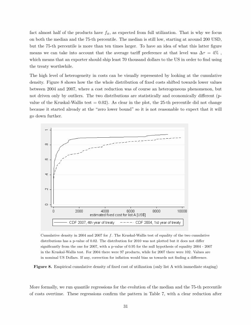
fact almost half of the products have fit, as expected from full utilization. That is why we focuson both the median and the 75-th percentile. The median is still low, starting at around 200 USD,but the 75-th percentile is more than ten times larger. To have an idea of what this latter figuremeans we can take into account that the average tariff preference at that level was ∆τ = 4% ,which means that an exporter should ship least 70 thousand dollars to the US in order to find usingthe treaty worthwhile.

The high level of heterogeneity in costs can be visually represented by looking at the cumulativedensity. Figure 8 shows how the the whole distribution of fixed costs shifted towards lower valuesbetween 2004 and 2007, where a cost reduction was of course an heterogeneous phenomenon, butnot driven only by outliers. The two distributions are statistically and economically different (p-value of the Kruskal-Wallis test = 0.02). As clear in the plot, the 25-th percentile did not changebecause it started already at the “zero lower bound” so it is not reasonable to expect that it willgo down further.

Cumulative density in 2004 and 2007 for f . The Kruskal-Wallis test of equality of the two cumulativedistributions has a p-value of 0.02. The distribution for 2010 was not plotted but it does not differsignificantly from the one for 2007, with a p-value of 0.95 for the null hypothesis of equality 2004 - 2007in the Kruskal-Wallis test. For 2004 there were 97 products, while for 2007 there were 102. Values arein nominal US Dollars. If any, correction for inflation would bias us towards not finding a difference.

Figure 8. Empirical cumulative density of fixed cost of utilization (only list A with immediate staging)

More formally, we run quantile regressions for the evolution of the median and the 75-th percentileof costs overtime. These regressions confirm the pattern in Table 7, with a clear reduction after

31

the first year of the treaty. The third quartile decreases of utilization costs decreased by around70%, from circa 3,000 USD to below 1,000; with an additional decrease in the second year thatis borderline significant at 90%. But then it remains in the neighborhood between zero and athrousand dollars for the rest of our sample, even years 4 and 5 which coincide with the financialcrisis. The quantile regression for the median shows a very similar picture, with a large drop in thefirst year, although at much lower levels.

Plotted marginal effects using delta method for a quantile regression of utilization costs fit over various years t;estimated for the 75-th and 50-th percentiles. The 25-th percentile is not estimated because it precisely is zerofor all years. Plotted standard errors at 95% confidence.

Figure 9. Quantile regressions of the evolution of fixed cost by year

In the appendix we show additional robustness checks for our stylized fact of an important decreasein utilization costs, using standard regressions with product fixed effects and also taking into accountthe churning of products. All show a reduction in fixed costs

Overall, the estimates in this section are evidence consistent with some “learning” during the firstyears of the treaty, because the cutoff level needed for using the treaty went down both economicallyand statistically. We cannot distinguish, though, whether this process of reduction in the cutoff

32

size to use the treaty is due to learning within firms, market dynamics or externalities. 21

7 Concluding remarks.

This paper offers a model to explain why free trade agreements are not fully used, and then providea novel empirical technique to back out the fixed costs from data readily available to governments.

Our model is composed of exporters with heterogeneous productivity from a small open economy,who are price takers. When there are fixed costs of using the tariff benefits of a treaty, firms wouldweigh the benefits of doing it, which grows with the volume exported and the magnitude of thetariff advantage, against the fixed utilization costs. As usual in these models, larger exporters wouldprefer to use the treaty - increasing even more their shipments - while the smallest would rationallyrestraint from using the tariff benefit. In extreme cases, when the factor prices are not perfectlyelastic, the small exporters could even lose from the mere existence of the free trade agreement,since larger firms would use it, increasing exports and therefore pushing up factor prices. Thisdifferential utilization of the treaty is, at the best of our knowledge, a novel channel that createsheterogeneous impacts of free trade agreements within an industry.

We also offer a novel method to structurally estimate fixed utilization costs. Assuming that largerexporters in an industry use the treaty first, then we can back out which is the marginal exporterthat might be indifferent between using and not using the treaty. Since we observe its exportvolume and know the tariff savings from using the treaty, then we can back out the money that thismarginal user is apparently leaving on the table if it does not use it. This provides our estimatesfor the fixed cost.

Empirically, we estimate our model using data from Chilean firms exporting to the US, followingthe first years of the Free Trade Agreements between these two countries, starting in 2004. We findthat there is substantial heterogeneity across products. While for almost half of the products thecost was estimated to be zero or non binding for any firm, for the 75-th percentile the utilizationcost was around 3 thousand dollars. Given a tariff benefit of 4%, which is close to the mean in oursample, it means that treaty users would have to ship at least 70,000 dollars to the US to use thetreaty. We also find that the utilization cost is decreasing over time, especially in the first years, inwhich we observe a drop of around 70% for both the second and third quartiles of the distribution.These results are consistent with learning about the treaty.

21As a robustness check, in an analysis not shown here, we did not see any obvious differences in the abovementioned pattern of “learning” when we split the sample between sectors with stronger and weaker rules of origin.This may be partially explained by the concerns about endogenous rules of origin, biased towards more competitiveproducts and already discussed previously.

33

ReferencesAnson, J., O. Cadot, A. Estevadeordal, J. d. Melo, A. Suwa-Eisenmann, and B. Tu-

murchudur (2005): “Rules of Origin in North-South Preferential Trading Arrangements withan Application to NAFTA,” Review of International Economics, 13(3), 501–517.

Baldwin, R. E., and A. J. Venables (1995): “Chapter 31 Regional economic integration,” 3,1597 – 1644.

Berry, S., J. Levinsohn, and A. Pakes (1995): “Automobile prices in market equilibrium,”Econometrica: Journal of the Econometric Society, pp. 841–890.

Carrere, C., and J. de Melo (2004): “Are Different Rules of Origin Equally Costly? Estimatesfrom NAFTA,” (4437).

Demidova, S., and K. Krishna (2007): “Firm Heterogeneity and Firm Behavior with ConditionalPolicies,” (12950).

Freund, C. L., and E. Ornelas (2010): “Regional Trade Agreements,” World Bank PolicyResearch Working Paper No. 5314.

Hayakawa, K. (2011): “Measuring fixed costs for firms’ use of a free trade agreement: Thresholdregression approach,” Economics Letters, 113(3), 301 – 303.

Hayakawa, K., D. Hiratsuka, K. Shiino, and S. Sukegawa (2009): “Who Uses Free TradeAgreements?,” (DP-2009-22).

James, W. (2007): “Rules of origin in emerging Asia-Pacific preferential trade agreements: WillPTAs promote trade and development?,” Chapter IV in ESCAP. Trade facilitation beyond themultilateral trade negotiations: Regional practices, customs valuation and other emerging issues- A study by the Asia-Pacific Research and Training Network on Trade, pp. 137–159.

Ju, J., and K. Krishna (2002): “Regulations, regime switches and non-monotonicity when non-compliance is an option: an application to content protection and preference,” Economics Letters,77(3), 315 – 321.

Kohpaiboon, A. (2008): “Exporters’ Response to AFTA Tariff Preferences: Evidence from Thai-land,” mimeo.

Maggi, G., and A. Rodríguez-Clare (2007): “A Political-Economy Theory of Trade Agree-ments,” The American Economic Review, 97(4), pp. 1374–1406.

Melitz, M. J. (2003): “The impact of trade on intra-industry reallocations and aggregate industryproductivity,” Econometrica, pp. 1695–1725.

Olley, G. S., and A. Pakes (1996): “The Dynamics of Productivity in the TelecommunicationsEquipment Industry,” Econometrica, 64(6), pp. 1263–1297.

Takahashi, K., and S. Urata (2008): “On the Use of FTAs by Japanese Firms,” RIETI Dis-cussion Paper.

(2009): “On the Use of FTAs by Japanese Firms:Further evidence,” RIETI DiscussionPaper.

34

8 Appendix on how we built our sample

8.1 Explanation

Our analysis requires the use of a few datasets. The original data, prepared by the IADB, containssix variables: “HTSProductCode”, “HTSNumberExplanation”, “MFN”, “FTA”, “TotalTrade”, and“year”. “HTSProductCode” is the 8-digit code which identifies each product. “HTSNumberExpla-nation” contains a brief description of each product. “MFN” is the amount of trade that entersthe US through most favored nation status while “FTA” is the amount of trade that enters the USthrough the use of the FTA. “TotalTrade” is the sum of “MFN” and “FTA.” We also used infor-mation from Annex 3.3 of the FTA compiled into an Excel spreadsheet. This spreadsheet containsthe following variables: HTS2003, an identifying code for each product; description, which gives abrief description of each product; base rate, which contains the pre-FTA tariff rate; and staging,which identifies which tariff decrease schedule for each product. In order to account for the Rulesof Origin, we used a database which contained HSProductCode, an identifier at the 6 digit levelof each product, and the Rules of Origin description. For tariff rates, we used two sources: theUSITC and TRAINS tariffs datasets. The USITC dataset is identified on the HTS level whlie theTRAINS dataset is identified on the HS level.

Since there was not a common identifier across all datasets, the best merging strategy was notcompletely obvious. Through trial and error, we were able to come up with a workable method.In an ideal world, we would have had databases which all had the HTS 8-digit format as providedfor in the original database compiled by IADB. Since the databases do not all share a commonidentification code, we had to build in some translations so that the merge would work properly.After removing 75 duplicates from the original data, we merged the original database using theAnnex 3.3 database of stagings. Initially, it is not a perfect merge. We recover the nonmatchesthrough the use of the HS translator and the USITC tariffs data. When we apply the translator, welose some uniqueness. To resolve any problems with inconsistent stagings on the HS level, we usethe mode of the staging by each HS product code. These recovered observations are then appendedto the original database. This merge produces a loss of 11 observations. Next, we merge the Rulesof Origin database. 70 observations are lost as a result of this merge. Last, we merge the TRAINStariffs database which turns out to be a perfect merge. Altogether, we lose 234 observations throughthis merging process which yields a final total of 8,956 observations.

8.2 Detail of variable definition

useit =

0 ifuit = 0

1 ifuit > 0

35

fulluseit =

0 if 0 < uit < .90

1 ifuit > .90

logV alueit = ln(TotalTradeit)

ratediffit = MFNit − FTAit

ROOnestit =

1 if Cambio de Subpartida

2 if Cambio dePartida

3 if Cambio de Item

4 if Cambio deCapı́tulo

requisitoit =

1 if product has requisito de procesamiento

0 otherwise

V CRit =

1 if product has regional value content requirement

0 otherwise

quotait =

1 if product has import quota

0 otherwise

Persistence: “1” if a product enters in year t and is consistently exported for all subsequentyears; “0” otherwise.

9 Robustness checks on the decrease of utilization costs

This subsection makes additional analysis to confirm the robustness of the decrease in utilizationcosts over time. Regression show that f decreased between 10 and 20% per year during the period2004-2010, as shown in Table 8, but much more in the early years. First in specifications (1) and (2)we estimated a regression of ln (f + 1)to include observations with f = 0, showing a rate of declineper year of around 7 to 13 percentage points, depending on the type of fixed effects used. Whenlooking only among those products with non-zero the point estimates are even stronger, around20% reduction in utilization costs per year (3 and 4). Finally, specification (5) shows that most of

36

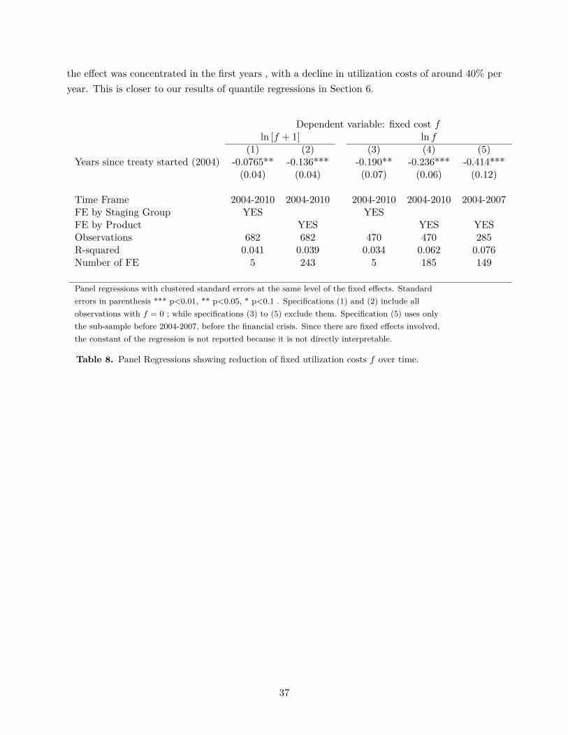
the effect was concentrated in the first years , with a decline in utilization costs of around 40% peryear. This is closer to our results of quantile regressions in Section 6.

Dependent variable: fixed cost fln [f + 1] ln f

(1) (2) (3) (4) (5)Years since treaty started (2004) -0.0765** -0.136*** -0.190** -0.236*** -0.414***

(0.04) (0.04) (0.07) (0.06) (0.12)

Time Frame 2004-2010 2004-2010 2004-2010 2004-2010 2004-2007FE by Staging Group YES YESFE by Product YES YES YESObservations 682 682 470 470 285R-squared 0.041 0.039 0.034 0.062 0.076Number of FE 5 243 5 185 149

Panel regressions with clustered standard errors at the same level of the fixed effects. Standarderrors in parenthesis *** p<0.01, ** p<0.05, * p<0.1 . Specifications (1) and (2) include allobservations with f = 0 ; while specifications (3) to (5) exclude them. Specification (5) uses onlythe sub-sample before 2004-2007, before the financial crisis. Since there are fixed effects involved,the constant of the regression is not reported because it is not directly interpretable.

Table 8. Panel Regressions showing reduction of fixed utilization costs f over time.

37

10 Appendix: Parameters of the Free Trade Agreementsbetween Chile and the US

Table 9. Staging list for the Chile-US FTA, indicating the reduction in tariff over the MFN tariff rate,so percentages are

(1− τF T A

t

)/τMF N

t .

Year2004 2005 2006 2007 2008 2009 2010 2011 2012 2013 2014 2015 NTheo %Theo

Product ListList A 100% 5,935 55.83List B 25% 50% 75% 100% 200 1.88List C 13% 25% 38% 50% 63% 75% 88% 100% 139 1.31List D 10% 20% 30% 40% 50% 60% 70% 80% 90% 100% 51 0.48List E 8% 17% 25% 33% 42% 50% 58% 67% 75% 83% 92% 100% 38 0.36List F “Free” , meaning that MFN tariff was already zero before the treaty 3,991 37.54List G 0% 0% 0% 0% 8% 17% 25% 33% 50% 67% 83% 100% 16 0.15List H 0% 0% 13% 25% 38% 50% 63% 75% 88% 100% 0 0List J 0% 0% 0% 0% 0% 0% 0% 20% 40% 60% 80% 100% 0 0List K 50% 50% 0 0List L 5% 10% 15% 20% 25% 30% 40% 50% 60% 100% 17 0.16List M 0% 0% 0% 0% 0% 0% 0% 0% 0% 100% 4 0.04List N 100% 23 0.22Annex 1 Special but usually “slow” 217 2.08Total 10,631 100

38