why is productivity procyclical? why do we care? · 7 why is productivity procyclical? why do we...

This PDF is a selection from an out-of-print volume from the National Bureauof Economic Research

Volume Title: New Developments in Productivity Analysis

Volume Author/Editor: Charles R. Hulten, Edwin R. Dean and Michael J.Harper, editors

Volume Publisher: University of Chicago Press

Volume ISBN: 0-226-36062-8

Volume URL: http://www.nber.org/books/hult01-1

Publication Date: January 2001

Chapter Title: Why Is Productivity Procyclical? Why Do We Care?

Chapter Author: Susanto Basu, John Fernald

Chapter URL: http://www.nber.org/chapters/c10128

Chapter pages in book: (p. 225 - 302)

�7Why Is Productivity Procyclical?Why Do We Care?

Susanto Basu and John Fernald

Productivity is procyclical. That is, whether measured as labor productiv-ity or total factor productivity, productivity rises in booms and falls inrecessions. Recent macroeconomic literature views this stylized fact of pro-cyclical productivity as an essential feature of business cycles, largely be-cause of the realization that each explanation for this stylized fact has im-portant implications for the workings of macroeconomic models. In thispaper, we seek to identify the empirical importance of the four main expla-nations for this stylized fact, and discuss the implications of our results forthe appropriateness of different macroeconomic models.

Until recently, economists generally regarded the long-run average rateof productivity growth as important for growth and welfare; procyclicalproductivity, by contrast, seemed irrelevant for understanding businesscycles. Economists presumed that high-frequency fluctuations in produc-tivity reflected cyclical mismeasurement—for example, labor and capitalworked harder and longer in booms—but these cyclical variations in utili-zation were not themselves important for understanding cycles.

In the past decade and a half, productivity fluctuations have taken cen-ter stage in modeling output fluctuations, and are now viewed as an essen-

Susanto Basu is associate professor of economics at the University of Michigan and aresearch associate of the National Bureau of Economic Research. John Fernald is senioreconomist at the Federal Reserve Bank of Chicago.

We are grateful for comments from Zvi Griliches, John Haltiwanger, Michael Horvath,Charles Hulten, Dale Jorgenson, Catherine Morrison, Plutarchos Sakellaris, and partici-pants in the conference. Basu thanks the National Science Foundation and the Alfred P.Sloan Foundation for financial support. The views in this paper are solely the responsibilityof the authors and should not be interpreted as reflecting the views of the Board of Governorsof the Federal Reserve System or of any other person associated with the Federal ReserveSystem.

225

tial part of the cycle. Figure 7.2 (discussed later) charts the Solow residualfor the aggregate U.S. economy. The figure also shows growth in outputand growth in “inputs,” defined as a weighted average of labor and capitalgrowth (we discuss data sources and definitions in section 7.4). Mean pro-ductivity growth is positive, so that over time society’s ability to producegoods or services that satisfy final demand is rising faster than its inputs.In addition, productivity growth is quite volatile. The volatility is not ran-dom, but is significantly procyclical: The correlation with output growthis about 0.8.

Macroeconomists have become interested in the cyclical behavior ofproductivity because of the realization that procyclicality is closely relatedto the impulses or propagation mechanisms underlying business cycles.Even the cyclical mismeasurement that was formerly dismissed as unim-portant turns out to be a potentially important propagation mechanism.

There are four main explanations for high-frequency fluctuations in pro-ductivity. First, procyclical productivity may reflect procyclical technol-ogy. After all, under standard conditions, total factor productivity mea-sures technology. If there are high-frequency fluctuations in technology, itis not surprising that there are high-frequency fluctuations in output aswell. Second, widespread imperfect competition and increasing returnsmay lead productivity to rise whenever inputs rise. (Increasing returnscould be internal to a firm, or could reflect externalities from the activityof other firms.) Figure 7.2 (discussed later) shows the key stylized fact ofbusiness cycles, the comovement of inputs and output. With increasingreturns, the fluctuations in inputs then cause endogenous, procyclical fluc-tuations in productivity. Third, as already mentioned, utilization of inputsmay vary over the cycle. Fourth, reallocation of resources across uses withdifferent marginal products may contribute to procyclicality. For example,if different industries have different degrees of market power, then inputswill generally have different marginal products in different uses. Then ag-gregate productivity growth is cyclical if sectors with higher markups haveinput growth that is more cyclical. Alternatively, if inputs are relativelyimmobile or quasi-fixed, then marginal products may temporarily differacross uses; as these resources eventually shift, productivity rises.1

Why do economists now care about the relative importance of these fourexplanations? In large part, changes in the methodology of macroeconom-ics have raised the fact of procyclical productivity to the forefront. Ma-croeconomists of all persuasions now use dynamic general equilibrium(DGE) models, and it turns out that each of the four explanations hasimportant implications for the workings of these models. Hence, answering

1. For examples of these four explanations, see, respectively, Cooley and Prescott (1995);Hall (1988, 1990); Basu (1996), Bils and Cho (1994), and Gordon (1993); and Basu andFernald (1997a, 1997b).

226 Susanto Basu and John Fernald

why productivity is procyclical sheds light on the relative merits of differ-ent models of the business cycle.

First, if high-frequency fluctuations in productivity reflect high-frequency fluctuations in technology, then comovement of output and in-put (i.e., business cycles) are a natural byproduct. The DGE approach tobusiness cycle modeling began with so-called real business cycle models,which explore the extent to which the frictionless one-sector Ramsey-Cass-Koopmans growth model can explain business cycle correlations. Realbusiness cycle models use Solow’s productivity residual—interpreted asaggregate technology shocks—as the dominant impulse driving the cycle(e.g., Cooley and Prescott 1995). Other impulses may affect output in thesemodels, but technology shocks must dominate if the model is to match thekey stylized fact of business cycles: the positive comovement of output andlabor input.2

Second, recent papers show that increasing returns and imperfect com-petition can modify and magnify the effects of various shocks in an other-wise standard DGE model. In response to government demand shocks,for example, models with countercyclical markups can explain a rise in realwages while models with increasing returns can explain a rise in measuredproductivity. Perhaps most strikingly, if increasing returns are largeenough, they can lead to multiple equilibria, in which sunspots or purelynominal shocks drive business cycles.3 Furthermore, if firms are not allperfectly competitive, then it is not appropriate to use the Solow residualas a measure of technology shocks, since the Solow residual becomes en-dogenous. Taking the Solow residual to be exogenous thereby mixes im-pulses and propagation mechanisms.

Third, variable utilization of resources turns out to improve the propa-gation of shocks in DGE models. If firms can vary the intensity of factoruse, then the effective supply of capital and labor becomes more elastic.Small shocks (to technology or demand) can then lead to large fluctua-tions.4 If the model has sticky nominal prices, these elastic factor suppliesgreatly increase the persistence of the real effects of nominal shocks.

Fourth, reallocations of inputs, without any change in technology, maycause aggregate productivity to be procyclical. For example, in the sectoral

Why Is Productivity Procyclical? Why Do We Care? 227

2. Barro and King (1984) provide an early discussion of this issue. Dynamic general equi-librium models without technology shocks can match this stylized fact with countercyclicalmarkups of price over marginal cost, arising from sticky prices (as in Kimball, 1995) or fromgame-theoretic interactions between firms (as in Rotemberg and Woodford 1992). Modelswith an extreme form of increasing returns—increasing marginal product of labor—can alsoproduce a positive comovement between output and labor input; see, for example, Farmerand Guo (1994).

3. See, for example, Rotemberg and Woodford (1992), Farmer and Guo (1994), andBeaudry and Devereux (1994). Rotemberg and Woodford (1995) survey dynamic generalequilibrium models with imperfect competition.

4. See, for example, Burnside and Eichenbaum (1996); Dotsey, King, and Wolman (1997);and Wen (1998).

shifts literature (e.g., Ramey and Shapiro 1998 and Phelan and Trejos1996), demand shocks cause differences in the marginal product of immo-bile factors across firms. Output fluctuations then reflect shifts of resourcesamong uses with different marginal products. Basu and Fernald (1997a)provide a simple stylized example in which aggregation over constant-returns firms with different levels of productivity lead to the existence ofmultiple equilibria. Weder (1997) calibrates a DGE model where durablesmanufacturing firms have increasing returns while all other producershave constant returns (calibrated from results in Basu and Fernald 1997a),and shows that reallocations make multiple equilibria possible in thatmodel. Of course, reallocations can also help propagate sector-specifictechnology shocks, as in Lilien (1982).

In this paper, we seek to identify the importance of the four explana-tions. Our approach builds on the seminal contributions of Solow (1957)and Hall (1990). We allow for imperfect competition and nonconstant re-turns to scale, as well as variations in the workweek of capital or the effortof labor that are unobservable to the econometrician. In the Solow-Halltradition, we take the production function residual as a measure of sectoraltechnology shocks. We then aggregate over sectors, since our ultimate fo-cus is on explaining movements in aggregate productivity.

Our empirical work relies primarily on the tools developed by Basu andFernald (1997b) and Basu and Kimball (1997). Both papers allow for in-creasing returns to scale and markups of price over marginal cost. Basuand Fernald stress the role of sectoral heterogeneity. They argue that foreconomically plausible reasons—for example, differences across industriesin the degree of market power—the marginal product of an input maydiffer across uses. Then aggregate productivity growth depends in part onwhich sectors change inputs.

Basu and Kimball stress the role of variable capital and labor utilization.Solow’s original (1957) article presumed that variations in capacity utiliza-tion were a major reason for the procyclicality of measured productivity,a presumption widely held thereafter. (See, for example, Gordon 1993; Ab-bott, Griliches, and Hausman 1998). In essence, the problem is cyclicalmeasurement error of input quantities: True inputs are more cyclical thanmeasured inputs, so that measured productivity is spuriously procyclical.

Basu and Kimball use the basic insight that a cost-minimizing firm op-erates on all margins simultaneously—whether observed or unobserved—ensuring that the marginal benefit of any input equals its marginal cost.As a result, increases in observed inputs can proxy for unobserved changesin utilization. For example, when labor is particularly valuable, firms willwork existing employees both longer (increasing observed hours perworker) and harder (increasing unobserved effort).

Our work on these issues follows the Solow-Hall tradition, which makesminimal assumptions and focuses on the properties of the resulting resid-


ual. An alternative literature, surveyed by Nadiri and Prucha (ch. 4, thisvolume), addresses issues of technology change by attempting to estimatean extensively parameterized production (or cost) function. That approachcan address a wider range of issues because it imposes much more struc-ture on the problem. If the problem is correctly specified and all necessarydata are available, the more parametric approach offers clear theoreticaladvantages, since one can then estimate second-order properties of theproduction function such as elasticities of substitution. However, that ap-proach is likely to suffer considerable practical disadvantages, such as theincreased likelihood of misspecification and the necessity of factor pricesbeing allocative period by period. We are skeptical that observed factorprices are always allocative—with implicit contracts, for example, ob-served wages need only be right on average, rather than needing to beallocative period by period. Hence, we argue in favor of an explicitly first-order approach when possible, since results are likely to be more robust.

Note that this production function literature sometimes claims to solvethe capacity utilization problem (e.g., Morrison 1992a,b). Suppose, forexample, that the capital stock cannot be changed instantaneously but thatit is nevertheless used all the time. It can still be used more intensively bycombining the fixed capital services with more labor and materials. As aresult, the shadow value of this quasi-fixed capital stock may vary from itslong-run equilibrium factor cost. Capital’s output elasticity may also varyover time, reflecting variations in this shadow value. More generally, withquasi-fixity, quantities of inputs (and output) may differ from long-runequilibrium values; similarly, on the dual (cost) side, short-run variablecost may differ from long run variable cost at a given output level. If weequate full capacity with the firm’s optimal long-run equilibrium point,then capacity utilization (defined by how far actual output or variable costis from their appropriately-defined long-run equilibrium values) may varyover time.

For estimating the technology residual, the relevant feature of this litera-ture is that it attempts to estimate the shadow value of quasi-fixed inputsin order to calculate the time variation in the output elasticities. The pro-duction function literature thus tries to control for time-varying outputelasticities, while the capacity-utilization literature tries to measure factorquantities (i.e., the service flow) correctly.5

The enormous confusion between these two logically distinct ideasstems purely from the semantic confusion caused by both literaturesclaiming to address the capacity utilization problem. In particular, adher-ents of the time-varying elasticity approach often claim that their opti-


5. For our purposes, this is the only difference that matters. The structural literature alsoestimates a variety of other quantities, such as elasticities of substitution, that may be ofindependent interest.

mization-based methods obviate the need to use proxies that control forunobserved variations in capital workweek or labor effort, with the impli-cation that the use of proxies is somehow ad hoc. This implication iswrong. The production function literature assumes that the quantities ofall inputs are correctly measured; the capacity utilization literature devotesitself to correcting for measurement error in the inputs. The two addressseparate issues.

The easiest way to see the difference between the two concepts is tosuppose that output is produced via a Cobb-Douglas production function.Then the output elasticities are constant, so for our purposes—for ex-ample, estimating returns to scale—the time-varying elasticity literaturehas nothing to add. But there is still a capacity utilization problem—forexample, if workers work harder in a boom than in recessions, but this factis not captured in the statistics on labor input. Formally, therefore, theproblem of time-varying elasticities is a second-order issue—it relates todeviations from the first-order Cobb-Douglas approximation—but capac-ity utilization is a first-order issue, since it concerns the accurate measure-ment of the inputs.

After presenting empirical results, we discuss implications for macro-economics. We discussed some of these implications above, in motivatingour interest in procyclical productivity, so we highlight other issues. Norm-ative productivity analysis emphasizes the welfare interpretation of theproductivity residual. But what if productivity and technology differ be-cause of distortions such as imperfect competition? Recent macroeco-nomic literature often seems to assume that we measure productivity inorder to measure technology; any differences reflect mismeasurement. Al-though variable input utilization is clearly a form of mismeasurement, weargue that other distortions (such as imperfect competition) are not: Pro-ductivity has clear welfare implications, even in a world with distortions.A modified Solow residual—which reduces to Solow’s measure if thereare no economic profits—approximates to first order the welfare changeof a representative consumer. Intuitively, growth in aggregate output mea-sures the growth in society’s ability to consume. To measure welfarechange, we must then subtract the opportunity cost of the inputs used toproduce this output growth. Input prices measure that cost, even whenthey do not measure marginal products. Hence, if productivity and tech-nology differ, then productivity most closely indexes welfare.

Section 7.1 provides a relatively informal overview of the issues. Wehighlight key issues facing the empirical literature and make recommenda-tions. That section will allow the reader to proceed to the data and empiri-cal sections 7.4 and 7.5. However, some of our choices in section 7.1 re-quire more formal treatment to justify fully; section 7.2 provides thistreatment. Section 7.3 discusses aggregation from the firm to the economy-wide level. Section 7.4 discusses data, and section 7.5 presents results. Sec-


tion 7.6 discusses several macroeconomic implications of our results. Sec-tion 7.7 concludes.

7.1 Methods of Estimating Technical Change: Overview

Why do macroeconomists care about fluctuations in productivity? First,and perhaps foremost, productivity yields information about the aggregateproduction of goods and services in the economy. Second, productivityanalysis may provide information about firm behavior—for example, themarkup and its cyclicality, the prevalence of increasing returns to scale,and the factors determining the level of utilization.

There are several possible approaches to empirical productivity anal-ysis. Each has advantages and disadvantages. In this section, we assessthese alternatives, and make recommendations about key decisions facingan empirical researcher. We summarize the microeconomic foundations ofour preferred approach, which is in the spirit of Solow (1957) and Hall(1990). This discussion may satisfy the interests and needs of most readers,who can then proceed to the data and results. However, a full justificationof our approach requires a somewhat more technical discussion. We pres-ent that technical discussion in sections 7.2 and 7.3.

Our ultimate goal is to understand the aggregate economy. At an aggre-gate level, the appropriate measure of output is national expenditure ongoods and services, that is, GDP—the sum of consumption, investment,government purchases, and net exports. GDP measures the quantity ofgoods available to consume today or invest for tomorrow. GDP is intrinsi-cally a value-added measure, since the national accounts identity assuresus that when we aggregate firm-level value added (defined in nominalterms as total revenue minus the cost of intermediate inputs of materialsand energy; in real terms, gross output with intermediate inputs netted outin some way, as discussed in section 7.3), aggregate value added equalsnational expenditure. The economy’s resources for producing goods andservices are capital and labor.

Nevertheless, despite our interest in macroeconomic aggregates, weshould begin at the level where goods are actually produced: at the levelof a firm or even a plant. The appropriate measure of output for a firm isgross output—shoes, books, computers, haircuts, and so forth. Firms com-bine inputs of capital, labor, and intermediate goods (materials and energy)to produce this gross output.

Our goal, then, is to explore how firm-level production of gross outputtranslates into production of aggregate final expenditure. Macroecono-mists often assume an aggregate production function that relates aggregatefinal expenditure (value added) to inputs of capital and labor. For manypurposes, what matters is whether such a function provides at least a first-order approximation to the economy’s production possibilities—even if an


explicit aggregate function does not exist (as it rarely does). For example,in calibrating a dynamic general equilibrium model, one may care abouthow much aggregate output increases if the equilibrium quantity of laborincreases, and a first-order approximation should give the right magni-tude.6 We argue that in a world without frictions or imperfections, aggrega-tion is generally very clean and straightforward. However, with frictionsand imperfections such as imperfect competition or costs of reallocatinginputs, the assumption that an aggregate production function exists (evenas a first-order approximation) generally fails—but the failures are eco-nomically interesting. These failures also help explain procyclical produc-tivity.

7.1.1 The Basic Setup

We write the firm’s production function for gross output, Yi, in the fol-lowing general form:

( ) ( ˜ , ˜ , , )1 Y F K L M Tii

i i i i=

Firms use capital services Ki, labor services Li, and intermediate inputs ofmaterials and energy Mi. We write capital and labor services with tildes toremind ourselves that these are the true inputs of services, which may notbe observed by the econometrician. Ti indexes technology, which we defineto include any inputs that affect firm-level production but are not compen-sated by the firm. For example, Ti comprises both standard exogenoustechnological progress and any Marshallian externalities that may exist;we take technology as unobservable. (For simplicity, we omit time sub-scripts.)

The services of labor and capital depend on both raw quantities (hoursworked and the capital stock), and the intensity with which they are used.We define labor services as the product of the number of employees, Ni,hours worked per employee Hi, and the effort of each worker, Ei. We definecapital services as the product of the capital stock, Ki, and the utilizationof the capital stock, Zi. (For example, Ki might represent a particular ma-chine, whereas Zi represents the machine’s workweek—how many hoursit is operated each period). Hence, input services are:

( ) ˜ ,

˜ .

2 L E H N

K Z K

i i i i

i i i

=

=

We will generally assume that the capital stock and the number of employ-ees are quasi-fixed, so firms cannot change their levels costlessly.


6. However, DGE models usually also need to relate changes in factor prices (e.g., wages)to changes in the quantities of inputs. For this purpose, the first-order approximation is notsufficient: One also needs to know the elasticities of substitution between inputs in produc-tion, which is a second-order property.

Let the firm’s production function F i be (locally) homogeneous of arbi-trary degree i in total inputs. Constant returns then corresponds to thecase where i equals 1. Formally, we can write returns to scale in twouseful, and equivalent, forms. First, returns to scale equal the sum of out-put elasticities:

( )˜ ˜

,3 1 2 3i

ii

i

ii

i

ii

i

F K

Y

F L

Y

F M

Y= + +

where F iJ denotes the derivative of the production function with respect to

the Jth element (i.e., the marginal product of input J ). Second, assumingfirms minimize cost, we can denote the firm’s cost function by Ci(Yi). (Ingeneral, the cost function also depends on the prices of the variable inputsand the quantities of any quasi-fixed inputs, although we omit those termsfor simplicity here.) The local degree of returns to scale equals the inverseof the elasticity of cost with respect to output.7

( ) ( )( )

( )

( )/

( ),4 i i

i i

i i i

i i i

i i

i

i

YC Y

YC Y

C Y Y

C Y

AC

MC=

′=

′=

where ACi equals average cost, and MCi equals marginal cost. Increasingreturns, in particular, may reflect overhead costs or decreasing marginalcost; both imply that average cost exceeds marginal cost. If increasing re-turns take the form of overhead costs, then '(Yi) is not a constant struc-tural parameter, but depends on the level of output the firm produces. Asproduction increases, returns to scale fall as the firm moves down its aver-age cost curve.

As equation (4) shows, there is no necessary relationship between thedegree of returns to scale and the slope of the marginal cost curve. Indeed,increasing returns are compatible with increasing marginal costs, as in thestandard Chamberlinian model of imperfect competition. One can cali-brate the slope of the marginal cost curve from the degree of returns toscale only by assuming there are no fixed costs. An important point is thatthe slope of the marginal cost curve determines the slopes of the factordemand functions, which in turn are critical for determining the results ofDGE models (for example, whether the model allows sunspot fluctua-tions). Several studies have used estimates of the degree of returns to scaleto calibrate the slope of marginal cost; for a discussion of this practice, seeSchmitt-Grohe (1997).

Firms may also charge a price Pi that is a markup, �i, over marginalcost. That is, �i � Pi /MCi. Returns to scale i is a technical property ofthe production function, whereas the markup �i is essentially a behavioralparameter, depending on the firm’s pricing decision. However, from equa-tion (4), the two are inextricably linked:

7. See Varian (1984, 68) for a proof.


( )( )

( ) ( )

( )( ) ,5 1 � �i

i i

i i i

i

i i

i i

i ii i

C Y

YC Y

P

C Y

C Y

PYs=

′=

′= −

where s�i is the share of pure economic profit in gross revenue. As long aspure economic profits are small (and in our data, we estimate the averageprofit rate to be at most 3 percent8), equation (5) shows that �i approxi-mately equals i. Large markups, for example, require large increasing re-turns. This is just what one would expect if free entry drives profits to zeroin equilibrium—for example, in Chamberlinian monopolistic competition.Thus, although increasing returns and markups are not equivalent from awelfare perspective, they are forced to equal one another if competitioneliminates profits. As a result, as we show in the next subsection, one canwrite the resulting wedge between output elasticities and factor shares interms of either parameter. Given low estimated profits, equation (5) showsthat strongly diminishing returns (i much less than one) imply that firmsconsistently price output below marginal cost (�i less than one). Sinceprice consistently below marginal cost makes no economic sense, we con-clude that average firm-level returns to scale must either be constant orincreasing. Increasing returns also require that firms charge a markup, aslong as firms do not make losses.

7.1.2 The Solow-Hall Approach

Suppose we want to estimate how rapidly technology is changing. So-low’s (1957) seminal contribution involves differentiating the productionfunction and using the firm’s first-order conditions for cost minimization.If there are constant returns to scale and perfect competition, then thefirst-order conditions (discussed below) imply that output elasticities areobserved in the data by revenue shares. Hall (1988, 1990) extends Solow’scontribution to the case of increasing returns and imperfect competition.Under these conditions, output elasticities are not observed, since neitherreturns to scale nor markups are observed. However, Hall derives a simpleregression equation, which he then estimates. In this section, we extendHall’s approach by using gross-output data and taking account of variablefactor utilization.

We begin by taking logs of both sides of equation (1) and then differ-entiating with respect to time:

( ) ˜ ˜ .6 1 2 3dyF K

Ydk

F L

Ydl

F M

Ydm dti

ii

ii

ii

ii

ii

ii= + + +

Small letters denote growth rates (so dy, for example, equals (1/Y )Y ), andwe have normalized the output elasticity with respect to technology equalto one for simplicity.

8. Rotemberg and Woodford (1995) also provide a variety of evidence suggesting thatprofit rates are close to zero.


As Solow (1957) and Hall (1990) show, cost minimization puts addi-tional structure on equation (6), allowing us to relate the unknown outputelasticities to observed factor prices. In particular, suppose firms charge aprice Pi that is a markup, �i, over marginal cost. (The advantage of thecost minimization framework is that it is unnecessary to specify the poten-tially very complicated, dynamic profit maximization problem that givesrise to this price.) Perfect competition implies �i equals one. Suppose thatfirms take the price of all J inputs, PJi, as given by competitive markets.The first-order conditions for cost-minimization then imply that:

( ) .7 PF Pi Ji

i Ji= �

In other words, firms set the value of a factor’s marginal product equal toa markup over the factor’s input price. Equivalently, rearranging the equa-tion by dividing through by �i, this condition says that firms equate eachfactor’s marginal revenue product (Pi /�i)F i

J to the factor’s price.The price of capital, PKi, must be defined as the rental price (or shadow

rental price) of capital. In particular, if the firm makes pure economicprofits, these are generally paid to capital, since the owners of the firmtypically also own its capital. These profits should not be incorporatedinto the rental price. Equation (7) still holds if some factors are quasi-fixed, as long as we define the input price of the quasi-fixed factors as theappropriate shadow price, or implicit rental rate (Berndt and Fuss, 1986).We return to this point in section 7.2 where we specify a dynamic cost-minimization problem.

Using equation (7), we can write each output elasticity as the productof the markup multiplied by total expenditure on each input divided bytotal revenue. Thus, for example,

( ) .8 1F Z K

Y

P K

PYs

ii i

ii

Ki i

i ii Ki= ≡� �

(The marginal product of capital is F i1Zi, since the services from a machine

depend on the rate at which it is being utilized; i.e., its workweek.) Theshares sJi are total cost of each type of input divided by total revenue. Thus,the input shares sum to less than one if firms make pure profits.

We now substitute these output elasticities into equation (6) and use thedefinition of input services from equation (2):

dy s dk s dl s dm dt

s dk dz s dn dh de s dm dt

s dk s dn dh s dm s

s dz s de

s

i i Ki i Li i Mi i i

i Ki i i Li i i i Mi i i

i Ki i Li i i Mi i i Mi

Ki i Li i

Mi

= + + +

= + + + + + +

= + + + + −

+−

�

�

� �

[ ˜ ˜ ]

[ ( ) ( ) ]

[ ( ) ] ( )

( )

1

1 + dti


By defining dx as a share-weighted average of conventional (observed) in-put growth, and du as a weighted average of unobserved variation in capi-tal utilization and effort, we obtain our basic estimating equation:

( ) ( ) .9 1dy dx s du dti i i i Mi i i= + − +� �

Using equation (5), we could rewrite equation (9) in terms of returns toscale i. In that case, the correct weights to calculate weighted averageinputs are cost shares, which sum to one, rather than revenue shares, whichmight not. Hall (1990) used the cost-share approach, but there is no eco-nomic difference between Hall’s approach and ours, and the data require-ments are the same. In particular, once we allow for the possibility of eco-nomic profits, we must in any case estimate a required rental cost ofcapital. Writing the equation in terms of �i turns out to simplify some laterderivations and also facilitates the welfare discussion in Section VI.

Suppose all firms have constant returns to scale, all markets are per-fectly competitive, and all factor inputs are freely variable and perfectlyobserved. Then the markup �i equals one, dui is identically zero (or isobserved), and all factor shares are observed as data (since there are noeconomic profits to worry about). This case corresponds to Solow’s (1957)assumptions, and we observe everything in equation (9) except technologychange dti, which we can calculate as a residual. However, if Solow’s condi-tions fail, we can follow Hall (1990) and treat equation (9) as a regression.

An alternative to the Solow-Hall approach involves estimating manymore properties of the production function (equation [1])—Nadiri andPrucha (this volume) survey that approach. That approach requires muchmore structure on the problem. For example, one must usually postulatea functional form and specify the firm’s complete maximization problem,including all constraints. If the problem is correctly specified and all neces-sary data are available, that approach offers clear theoretical advantagesfor estimating the second-order properties of the production function.However, the structural approach may suffer considerable practical disad-vantages, such as the increased likelihood of misspecification and the needfor all factor prices to be allocative period by period. In any case, for thefirst-order issues we focus on here, it should give similar results. (If it doesnot, our view is that the Solow-Hall approach is probably more robust).

Regarding equation (9) as an estimating equation, one immediatelyfaces three issues. First, the econometrician usually does not observe utili-zation du directly. In particular, if capital and labor utilization vary, thengrowth rates of the observed capital stock and labor hours do not capturethe full service flows from those inputs. In the short run, firms can varytheir inputs of capital and labor only by varying utilization. In this case,the regression suffers from measurement error. Unlike classical measure-ment error, variations in utilization du are likely to be (positively) corre-


lated with changes in the measured inputs dx, leading to an upward biasin estimated elasticities. Below, we draw on recent work in the literatureon capacity utilization, when we attempt to control for variable serviceflow from inputs.

Second, should one take the output elasticities as constant (appropriatefor a Cobb-Douglas production function or for a first-order log linear ap-proximation), or time varying? That is, should one allow the markup andthe share weights in equation (9) to change over time? If the elasticities arenot truly constant over time, then treating them as constant may introducebias. However, as we discuss later, attempting to estimate the time-varyingshares may lead to more problems than it solves.

Third, even if the output elasticities are constant and all inputs are ob-servable, one faces the “transmission problem” noted by Marschak andAndrews (1944): The technical change term, dt, is likely to be correlatedwith a firm’s input choices, leading to biased OLS estimates. In principle,one can solve this problem by instrumenting, but the need to use instru-ments affects our choice of the appropriate technique for estimating equa-tion (6). (One might expect technology improvements to lead to an expan-sion in inputs, making the OLS bias positive; Gali 1999 and Basu, Fernald,and Kimball 1999, however, argue that there are theoretical and empiricalreasons to expect a negative bias.)

7.1.3 Empirical Implementation

We now discuss the empirical issues noted above, beginning with capac-ity utilization. In the estimating equation (9), we need some way to observeutilization growth du or else to control for the measurement error resultingfrom unobserved changes in utilization.

Our approach builds on the intuition that firms view all inputs (whetherobserved by the econometrician or not) identically. Suppose a firm wantsmore labor input but cannot instantaneously hire more workers. Then thefirm should equate the marginal cost of obtaining more services from theobserved intensive margin (e.g., working current workers longer hours)and from the unobserved intensive margin (working them harder eachhour). If the costs of increasing hours and effort are convex, firms willchoose to use both margins. Thus changes in an observed input—for ex-ample, hours per worker—provide an index of unobserved changes in theintensity of work. This suggests a regression of the form

( ) ,10 dy dx adh dti i i i i i= + +�

where dhi is the growth rate of hours per worker. Earlier work by Abbott,Griliches, and Hausman (1998) also runs this regression to control for uti-lization.

In section 7.2, we construct a dynamic model of variable utilization that


provides complete microfoundations for this intuition. That model showsthat the regression in equation (10) appropriately controls for variableeffort. In addition, if the cost of varying the workweek of capital takes theform of a shift premium—for example, one needs to pay workers more towork at night—then this regression corrects for variations in utilization ofcapital as well as effort. (If the cost of varying capital’s workweek is “wearand tear”—i.e., capital depreciates in use—then the regression is some-what more complicated.)

Variable utilization of inputs suggests two additional problems in esti-mating regressions like equations (9) or (10), both of which make it difficultto observe “true” factor prices at high frequencies. First, firms will varyutilization only if inputs of capital and labor are quasi-fixed—that is,costly to adjust. Varying utilization presumably costs the firm something—for example, a shift premium. Thus, if firms could vary the number ofmachines or workers without cost, they would always adjust along theseextensive margins rather than varying utilization. However, if inputs arecostly to adjust, then the shadow price of an input to the firm may notequal its current market price. For example, investment adjustment costsimply that the return to installed capital may differ from its frictionlessrental rate.

Second, varying utilization—especially of labor—is most viable whenworkers and firms have a long-term relationship. A firm may increase workintensity when demand is high, promising to allow workers a break in thenext downturn. Such a strategy cannot be implemented if most workers arenot employed by the firm when the next downturn comes. The existence ofsuch long-term relationships suggests that wages may be set to be right“on average,” instead of being the correct spot market wages in every pe-riod. Thus, both quasi-fixity and implicit labor contracts imply that wemay not be able to observe factor prices at high frequencies.

This inability to observe factor prices period by period implies that weprobably want to assume constant, rather than time-varying, elasticities.This is unfortunate, since the first-order equations (8) suggest that if factorshares vary over time, then output elasticities may vary as well. But if,because of quasi-fixity and implicit labor contracts, we do not observethe relevant shadow values, then observed shares do not tell us how theelasticities vary. For estimating the average markup, a first-order approxi-mation may suffice, and may be relatively unaffected by our inability to ob-serve factor prices at high frequency. Of course, if our goal were to esti-mate elasticities of substitution between inputs, then we would need to findsome way to deal with these problems—we could not use a first-order ap-proximation that simply assumes the elasticities are one.9

9. For example, Berman, Bound, and Griliches (1994) and others investigate the hypothesisthat technological progress is skill-biased, and hence contributed to the increase in incomeinequality in the United States in recent decades; Jorgenson (1987) argues that part of theproductivity slowdown of the 1970s and 1980s is due to energy-biased technical change.


With these considerations in mind, we now assess four methods of esti-mating the parameters in the production function. First, one can simplytake equation (6) as an estimating equation and estimate the output elas-ticities directly. This approach, which essentially assumes that the produc-tion function is Cobb-Douglas, can be justified as a first-order approxima-tion to a more general production function. But this procedure requires usto estimate three parameters (or more, if we include proxies for variableutilization) for the output elasticities using data that are often multicollin-ear, and also subject to differing degrees of endogeneity and hence differ-ing OLS biases. The use of instrumental variables is not a complete solu-tion, since most plausible instruments are relatively weak. The literatureon weak instruments suggests that instrumental-variables methods havedifficulty with multiple parameters; see, for example, Shea (1997).

Second, one can impose cost minimization and estimate equations (9)or (10), while still taking a first-order approximation. Cost minimizationis a relatively weak condition, and seems likely to hold at least approxi-mately. Imposing it allows us to move from estimating three parameters toestimating only one (the markup), thus increasing efficiency. (Of course,assuming a particular model of cost minimization, if it is inappropriate,can lead to specification error. For example, if firms are not price takers infactor markets—for example, if firms have monopsony power or, in gen-eral, face price-quantity schedules for their inputs rather than singleprices—then cost-minimizing conditions, and hence the Hall equations [9]or [10], are misspecified.)

In this case, one simply assumes that the shares used in constructing dxi

are constant, as is the markup, �i. As with the first approach, if our interestis in first-order properties such as average markups or returns to scale, itcan in principle give an accurate answer, although the omitted second-order terms may well be important. (Risk aversion is a second-order phe-nomenon, but there is an active insurance industry.) A substantial advan-tage of the first-order approach is that it does not require that observedfactor prices (or rental rates) be allocative in every period. The averageshares are likely to be close to the steady-state shares, so the approximationtypically will be correct even with quasi-fixed inputs or implicit contracts.

Third, one could continue to estimate equations (9) or (10), but allowthe shares to change period by period. If markups are constant, if factorprices are allocative period by period, and if there are no quasi-fixed fac-tors, then this approach can, in principle, give a second-order approxima-tion to any production function (Diewert 1976). If these conditions fail,then this approach in essence incorporates some second-order effects, butnot others; it is unclear whether this is preferable to including none ofthem.

Fourth, one could estimate a flexible, general functional form along withEuler equations for the quasi-fixed inputs; as Nadiri and Prucha (this vol-ume) discuss, this approach provides a complete second-order approxima-


tion to any production technology. If we properly parameterize the firm’sproblem, then the markup need not be constant, and factors can be quasi-fixed—the model provides estimates of the true shadow values. In prin-ciple, this full structural approach provides a complete characterization ofthe technology; one can then calculate elasticities of substitution, biasesof technological change, and so forth. For some macroeconomic questions,these parameters are crucial.10

However, this general approach has the disadvantage that one needs toestimate many parameters (a translog production function for equation[1], for example, has twenty-five parameters before imposing restrictions,to say nothing of the associated Euler equations). Efficient estimation re-quires various restrictions and identifying assumptions, such as estimatingthe first-order conditions (equation [7]) along with the production functionitself. Hence, results may be sensitive to misspecification. For example, ifwages are determined by an implicit contract, and hence are not allocativeperiod by period, then one would not want an approach that relies heavilyon high-frequency changes in observed factor prices (and hence factorshares) for identification. The structural approach can be estimated eitherthrough the production or cost function—that is, from the primal or thedual side. Our concerns apply to both. We discuss these issues at greaterlength in section 7.2.3.

Since our primary interest is in measures of technical change, averagereturns to scale, and the average markup, in this paper we follow the sec-ond approach outlined above, using an explicitly first-order approxima-tion. (In practice, this gives qualitatively similar results to the third ap-proach, which allows the factor shares to vary over time). This secondmethod is essentially the procedure of Hall (1990), generalized to includematerials input and controls for variable factor utilization. Although thisapproach allows us to estimate the parameters governing firm-level tech-nology and behavior, our ultimate interest is describing the evolution ofaggregates. Thus, we must take one more step and aggregate output growthacross firms.

7.1.4 Aggregation

So far, we have discussed production and estimation in terms of firm-level gross output. Our ultimate interest is in aggregate value added. Ingeneral, no aggregate production function exists that links aggregate out-put to aggregate inputs—but the relationship between these aggregatesremains of interest. It turns out that aggregation across firms can intro-duce a significant new source of procyclical productivity.

10. For example, a recent strand of business-cycle theory emphasizes the cyclical propertiesof markups as important propagation mechanisms for output fluctuations; see, for example,Rotemberg and Woodford (1992, 1995). Time-series variation in the markup is a second-order property that can only be estimated with a second-order (or higher) approximation tothe production function.


In section 7.3, we derive the following equation for aggregate output(value added) growth dv:

( ) .11 dv dx du R dtV V V= + + +�

�V is the average “value added” markup across firms, du is an appropri-ately weighted average of firm-level utilization rates, R represents variousreallocation (or aggregation) effects, and dtV is an appropriately weightedaverage of firm-level technology. dxV is an weighted average of the aggre-gate capital stock and labor hours. In all cases, the superscript V refersthe fact that aggregate output is a value-added measure rather than agross-output measure, which requires some minor changes in definitions.(As we discuss in section 7.3, for macroeconomic modeling it is the “value-added markup” that is likely to be of interest.)

The major implication of equation (11) is that output growth at the ag-gregate level is not completely analogous to output growth at the firmlevel. The firm-level equation (9) looks similar to equation (11). Firm-leveloutput growth depends on input growth, the markup, variations in utiliza-tion, and technical change; aggregate output growth depends on aggregateinput growth, the average markup, average variation in utilization, andaverage technical change. Equation (11), however, has a qualitatively newterm, R.

The reallocation term reflects the effect on output growth of differencesacross uses in the (social) values of the marginal products of inputs. Out-put growth therefore depends on the distribution of input growth as wellas on its mean: If inputs grow rapidly in firms where they have above-average marginal products, output grows rapidly as well. Thus, aggregateproductivity growth is not just firm-level productivity growth writ large.There are qualitatively new effects at the aggregate level, which may beimportant both for estimating firm-level parameters and as powerful am-plification and propagation mechanisms in their own right.

For example, suppose that some firms have large markups of price overmarginal cost while others have low markups. Also suppose that all firmspay the same prices for their factors. Then resources such as labor have ahigher marginal product in the firms with the larger markup, as shown bythe first-order condition (equation [8]). Intuitively, because these firmshave market power, they produce too little output and employ too fewresources; hence, the social value of the marginal product of these inputsis higher. The reallocation term R captures the fact that aggregate outputrises if resources shift from low- to high-markup firms.

To summarize this section, we argue in favor of the following approachto estimating technology change, controlling for utilization. First, interpretall results as first-order approximations, on the grounds that the data areprobably insufficient to allow reliable estimation of second-order approxi-mations. Second, estimate equation (10)—a Hall (1990)-style regression


with a theoretically justified utilization proxy—at a disaggregated level.Take the residuals as a measure of disaggregated technology change.Third, use the aggregation equation (11)—which incorporates the disag-gregated estimates of technology change, markups, and utilization—toidentify the importance of the various explanations for procyclical produc-tivity.

The casual reader is now well prepared to proceed to the data and em-pirical sections of this paper in sections 7.4 and 7.5. However, our discus-sion passed quickly over several technical details. To fully justify ourchoice of method, it is useful to address those issues in detail. We do so insections 7.2 and 7.3.

7.2 The Meaning and Measurement of Capacity Utilization

Section 7.1 raised several issues with empirical implementation of theSolow-Hall approach to estimating technology, markups, and variationsin utilization at a disaggregated level. First, we must decide what prices touse in calculating weights. With quasi-fixed inputs, the appropriate shadowprice is not, in general, the observed factor price. In addition, even if fac-tors are freely variable, the observed factor prices may not be allocative:For example, firms and workers may have implicit contracts. Second, wemust decide whether to use a first- or second-order approximation to thecontinuous time equation (10). Third, we must find suitable proxies for du.

This section provides explicit microfoundations for our preferred ap-proach. We specify a dynamic cost-minimization problem to provide ap-propriate shadow values. We then discuss the pros and cons of first- versussecond-order approximations. Finally, we use the first-order conditionsfrom the cost minimization problem to find observable proxies for un-observed effort and capital utilization.

We argue in favor of using an explicitly first-order approximation forthe estimating equation, on the grounds that the data necessary for anappropriate second-order approximation are unavailable. We also arguefor using growth in hours per worker to adjust for variations in effort andcapital utilization. We also spend some time clarifying conceptual confu-sions over the meaning of capacity utilization. In particular, we argue thatcorrecting for capacity utilization requires correcting quantities, notmerely output elasticities.

7.2.1 A Dynamic Cost-Minimization Problem

We now specify a particular dynamic cost-minimization problem. Al-though the problem is relatively complicated, specifying it provides insightinto several practical issues in attempting to estimate equation (10) inthe previous subsection, and, in section 7.2.4, provides proxies for un-observed utilization.


We model the firm as facing adjustment costs in both investment andhiring, so that both the amount of capital (number of machines and build-ings), K, and employment (number of workers), N, are quasi-fixed. Wemodel quasi-fixity for two reasons. First, we want to examine the effect ofquasi-fixity per se on estimates of production function parameters andfirm behavior. Second, quasi-fixity is necessary for a meaningful model ofvariable factor utilization. Higher utilization must be more costly to thefirm, otherwise factors would always be fully utilized. If there were no costto increasing the rate of investment or hiring, firms would always keeputilization at its minimum level and vary inputs using only the extensivemargin, hiring and firing workers and capital costlessly. Only if it is costlyto adjust along the extensive margin is it sensible to adjust along the inten-sive margin, and pay the costs of higher utilization.11

We assume that the number of hours per week for each worker, H, canvary freely, with no adjustment cost. In addition, both capital and laborhave freely variable utilization rates. For both capital and labor, the benefitof higher utilization is its multiplication of effective inputs. We assume themajor cost of increasing capital utilization, Z, is that firms may have topay a shift premium (a higher base wage) to compensate employees forworking at night, or at other undesirable times.12 We take Z to be a contin-uous variable for simplicity, although variations in the workday of capital(i.e., the number of shifts) are perhaps the most plausible reason for varia-tions in utilization. The variable-shifts model has had considerable empiri-cal success in manufacturing data, where, for a short period of time, onecan observe the number of shifts directly.13 The cost of higher labor utiliza-tion, E, is a higher disutility on the part of workers that must be compen-sated with a higher wage. We allow for the possibility that this wage isunobserved from period to period, as might be the case if wage paymentsare governed by an implicit contract in a long-term relationship.

Consider the following cost minimization problem for the representativefirm of an industry:


11. One does not require internal adjustment costs to model variable factor utilization inan aggregative model (see, e.g., Burnside and Eichenbaum, 1996), because changes in inputdemand on the part of the representative firm change the aggregate real wage and interestrate, so in effect the concavity of the representative consumer’s utility function acts as anadjustment cost that is external to the firm. However, if one wants to model the behavior offirms that vary utilization in response to idiosyncratic changes in technology or demand—obviously the case in the real world—then one is forced to posit the existence of internaladjustment costs in order to have a coherent model of variable factor utilization. (Both ofthese observations are found in Haavelmo’s 1960 treatment of investment.)

12. Our model can be extended easily to allow utilization to affect the rate at which capitaldepreciates, as in Basu and Kimball (1997). We consider the simpler case for ease of exposi-tion. Nadiri and Prucha (this vol.) show that their approach of estimating a second-orderapproximation to the production function can also accommodate variable depreciation, butdo not consider either a shift premium or variable labor effort.

13. See, for example, Beaulieu and Mattey (1998) and Shapiro (1996).

( ) ( ) [ ( , ) ( )

( / ) ( / )]

, , , , ,12 0

0

1

minZ E H M I A

rd

MC Y e WNG H E V Z P M

WN A N PKJ I K ds

s

= ∫ +

+ +

−∞

∫�

�

subject to

( ) ( , , , )13 Y F ZK EHN M T=

( ) ˙14 K I K= − �

( ) ˙15 N A=

The production function and inputs are as before. In addition, I is grossinvestment, and A is hiring net of separations. WG(H, E )V(Z ) is total com-pensation per worker (compensation may take the form of an implicitcontract, and hence not be observed period by period). W is the basewage; the function G specifies how the hourly wage depends on effort, E, andthe length of the workday, H; and V(Z ) is the shift premium. WN�(A/N ) isthe total cost of changing the number of employees; PI KJ(I/K ) is the totalcost of investment; PM is the price of materials; and � is the rate of depreci-ation. We continue to omit time subscripts for clarity.

Using a perfect-foresight model amounts to making a certainty equiva-lence approximation. However, even departures from certainty equiva-lence should not disturb the key results, which rely only on intratemporaloptimization conditions rather than intertemporal ones.

We assume that �, and J are convex and make the appropriate technicalassumptions on G in the spirit of convexity and normality.14 It is also help-ful to make some normalizations in relation to the normal or steady-statelevels of the variables. Let J(�) � �, J�(�) � 1, �(0) � 0. We also assumethat the marginal employment adjustment cost is zero at a constant levelof employment: ��(0) � 0.

We use the standard current-value Hamiltonian to solve the representa-tive firm’s problem. Let �, q, and � be the multipliers on the constraints inequations (13), (14), and (15), respectively. Numerical subscripts denotederivatives of the production function F with respect to its first, second,and third arguments, and literal subscripts denote derivatives of the la-bor cost function G. The six intratemporal first-order conditions for cost-minimization are

( ) : ( , , ; ) ( , ) ( ).16 1Z KF ZK EHN M T WNG H E V Z� = ′

( ) : ( , , ; ) ( , ) ( )17 2H ENF ZK EHN M T WNG H E V ZH� =


14. The conditions on G are easiest to state in terms of the function ! defined by ln G(H,E ) � !(ln H, ln E ). Convex ! guarantees a global optimum; assuming !11 � !12 and!22 � !12 ensures that optimal H and E move together.

( ) : ( , , ; ) ( , ) ( )18 2E HNF ZK EHN M T WNG H E V ZE� =

( ) : ( , , ; )19 3M F ZK EHN M T PM� =

( ) : ( / )20 A W A N� = ′�

( ) : ( / ).21 I q PJ I KI= ′

The Euler equations for the capital stock and employment are

( ) ˙ ( ) [ ( / ) ( / ) ( / )]22 1 1q r q ZF P J I K I K J I K= + − + − ′� �

( ) ˙ ( , ) ( )

[ ( / ) ( / ) ( / )].

23 2� � �= − +

+ − ′

r EHF WG H E V Z

W A N A N A N� �

Since � is the Lagrange multiplier associated with the level of output,one can interpret it as marginal cost. The firm internally values output atmarginal cost, so �F1 is the marginal value product of effective capitalinput, �F2 is the marginal value product of effective labor input, and �F3

is the marginal value product of materials input.15 We defined the markup,�, as the ratio of output price, and P, to marginal cost, so � equals

( ) ( ) .24 ��

= ′ =C YP

Note that equation (24) is just a definition, not a theory determining themarkup. The markup depends on the solution of the firm’s more complexprofit maximization problem, which we do not need to specify.

Equations (22) and (23) implicitly define the shadow (rental) prices oflabor and capital:

( ) ( ) ˙ [ ( / ) ( / ) ( / )]25 1 1� �ZF r q q P J I K I K J I K PK= + − + − ′ ≡

( ) ˙ ( , ) ( )

[ ( / ) ( / ) ( / )] .

26 2� � �EHF r WG H E V Z

W A N A N A N PL

= − +

+ − ′ ≡� �

As usual, the firm equates the marginal value product of each input toits shadow price. Note that with these definitions of shadow prices, theatemporal first-order condition in equation (7) holds for all inputs. Forsome intuition, note that equation (25) is the standard first-order equationfrom a q-model of investment. In the absence of adjustment costs, thevalue of installed capital q equals the price of investment goods PI, andthe “price” of capital input is then just the standard Hall-Jorgenson costof capital (r � �)PI. With investment adjustment costs, there is potentially


15. For the standard static profit-maximization problem, of course, marginal cost equalsmarginal revenue, so these are also the marginal revenue products.

an extra return to owning capital, through capital gains q (as well as extraterms reflecting the fact that investing today raises the capital stock, andthus lowers adjustment costs in the future).

The intuition for labor in equation (26) is similar. Consider the casewhere labor can be adjusted freely, so that it is not quasi-fixed. Then ad-justment costs # are always zero. So is the multiplier �, since the constraintin equation (15) does not bind. In this case, as we expect, equation (26)says that the shadow price of labor input to the firm—the right side of theequation—just equals the (effort adjusted) compensation WG(H, E )V(Z )received by the worker. Otherwise, the quasi-fixity implies that the shadowprice of labor to a firm may differ from the compensation received bythe worker.

7.2.2 First-Order Approximations

We now turn to issues of estimation. This subsection discusses how toimplement our preferred first-order approximation; the next subsectioncompares this approach with second-order approximations.

Equations (6) and (9) hold exactly in continuous time, where the valuesof the output elasticities adjust continuously. In discrete time, we can inter-pret these equations as first-order approximations (in logs) to any generalproduction function if we assume the elasticities are constant. For a consis-tent first-order approximation to equation (9), one should interpret it asrepresenting small deviations from a steady-state growth path, and evalu-ate derivatives of the production function at the steady-state values of thevariables. Thus, to calculate the shares in equation (9), one should usesteady-state prices and quantities, and hence treat the shares as constantover time. The markup is then also taken as constant.

For example, in the first order approach, we want the steady-state out-put elasticity for capital, up to the unknown scalar �. Using asterisks todenote steady-state values, we use equations (21) and (25) and our normal-izations to compute the steady-state output elasticity of capital:

( )* * *

**

* *

* ** ( * ) * *

* *.27 1F Z K

Y

P K

P Y

r P K

P Y

K l= ≡ +� �

�

Note that the steady-state user cost of capital is the frictionless Hall-Jorgenson (1967) rental price.16 Since quasi-fixity matters only for the ad-justment to the steady state, in the steady state q � PI and q � 0. Opera-tionally, we calculate the Hall-Jorgenson user cost for each period and takethe time average of the resulting shares as an approximation to the steady-state share. We proceed analogously for the other inputs. In the final esti-


16. In practice, one would also include various tax adjustments. We do so in the empiricalwork, but omit them in the model to keep the exposition simple.

mating equation for equation (9), we use logarithmic differences in place ofoutput and input growth rates, and use steady-state shares for the weights.

Thus, we can construct the index of observable inputs, dx, and take theunknown �* multiplying it as a parameter to be estimated. We can use avariety of approaches to control for the unobserved du; we discuss someof them in section 7.2.4. Alternatively, under the heroic assumption thatdu is always zero or is uncorrelated with dx, we can estimate equation (9)while simply ignoring du. Hall (1988, 1990) and Basu and Fernald (1997a)follow this second procedure.

In any case, we have to use instruments that are orthogonal to the tech-nology shock dt, since technology change is generally contemporaneouslycorrelated with input use (observed or unobserved).17

7.2.3 Second-Order Approximations

The first-order approach of constant weights is, of course, equivalent toassuming that for small, stationary deviations from the steady-state bal-anced growth path, we can treat the production function as Cobb-Douglas. Parameters such as the average markup or degree of returns toscale are first-order properties, so the bias from taking a first-order ap-proximation may not be large.

Nevertheless, the Cobb-Douglas assumption is almost surely not liter-ally true. In principle, using a second-order approximation allows us toeliminate some of the bias in parameter estimates from using Cobb-Douglas and eliminate approximation errors that end up in the residual.It also allows us to estimate second-order properties of production func-tions, such as separability and elasticities of substitution. (Nadiri and Pru-cha, this volume) discuss the benefits of the second-order approach.)Unfortunately, the second order approach suffers severe practical disad-vantages—particularly the increased likelihood of misspecification. Ourview is that these sizeable disadvantages outweigh the potential benefits.

We begin this discussion with a simplest case where one obtains an ap-propriate second-order approximation to equation (9) simply by usingweights that change period by period. Suppose the production functiontakes a more general form than Cobb-Douglas, for example, translog.With a more general production function, output elasticities will typicallyvary over time if relative factor prices are not constant. Also suppose themarkup is constant, and that all factor shadow values (i.e., input prices)are observed, as will be the case if observed prices are allocative and thereare no costs of adjusting inputs. With a translog function (which provides aflexible approximation to any functional form), the discrete-time Tornqvist

17. Olley and Pakes (1996) propose an insightful alternative to the usual instrumental-variables approach; see Griliches and Mairesse (1998) for an excellent discussion of the prosand cons.


approximation to the continuous time equation (9) turns out to be exactlycorrect.18 This approximation requires replacing growth rates with logdifferences and replacing the continuous-time input shares with averageshares in adjacent periods. Thus, for example, the output elasticity for cap-ital is approximated by (1/2)(sKt � sKt�1), and is multiplied by the capitalchange term (ln Kt � ln Kt�1). In this case, using a Tornqvist index of inputuse allows a correct second-order approximation.

A major potential shortcoming with using changing shares is that ob-served factor prices may not be allocative period by period because ofimplicit contracts or quasi-fixity. Then observed factor shares might notbe proportional to output elasticities period by period, and the Tornqvistindex is misspecified.

A large literature has focused on the problem of quasi-fixity of capitaland labor, while largely ignoring the concern about implicit contracts. Webriefly review that approach to estimating second-order approximations.As discussed in the introduction, the time-varying elasticity literature—for example, Berndt and Fuss (1986), Hulten (1986), and the much moreparametric literature surveyed in Nadiri and Prucha (this volume)—triesexplicitly to deal with quasi-fixity. Quasi-fixity may lead to large variationsin input shadow prices, which in turn may cause the output elasticities tovary over time.19 The shadow prices may differ substantially from observedprices; in our cost-minimization setup of section 7.2.1, equations (25) and(26) show the relationship between shadow price and observed prices. Forexample, a firm may find that it has too many workers, so that the outputelasticity with respect to labor is very low. If the firm cannot (or choosesnot to) immediately shed labor, it will be forced to continue paying theseworkers. Then the observed labor share may be higher than the true outputelasticity, since the shadow value of labor is less than the wage.

Hulten (1986) shows that even with quasi-fixity, if there are constantreturns and perfect competition, then one can implement the Tornqvistapproximation to equation (9) using observed input prices and outputgrowth as long as there is only a single quasi-fixed input (e.g., capital).Under these conditions, the revenue shares sum to one. Since the observedinput prices give the correct shares for all inputs other than capital, capi-tal’s share can be taken as a residual. (As we emphasize again below, thisapproach corrects only for variations in the shadow values of quasi-fixedinputs, not unobserved changes in the workweek of capital.)


18. This result follows from Diewert (1976), who shows that the Tornqvist index is “super-lative”—that is, exact for functional forms such as the translog that are themselves flexibleapproximations to general functions—and shows that superlative indices have desirableindex-number properties. For discussions of the concept of “flexibility” and its limitations,see Lau (1986) and Chambers (1988, ch. 5).

19. As our previous discussion indicates, the output elasticities will generally change when-ever input prices (shadow values) change. Quasi-fixity is only one reason why shadow val-ues change.

Multiple quasi-fixed inputs cannot be accommodated using the non-parametric approach of equation (9), but one can estimate the parametersof a structural cost function. Pindyck and Rotemberg (1983) and Shapiro(1986), for example, estimate particular parametric forms of the produc-tion function along with Euler equations for the quasi-fixed inputs, suchas equations (22) and (23). As a by-product, this approach provides esti-mates of the shadow values of the state variables, and thus one can con-struct a measure of period-by-period shadow costs by valuing the input ofeach quasi-fixed factor at its shadow price.

The problem grows even more challenging when one allows for noncon-stant returns to scale. Since one cannot estimate the scale elasticity fromthe first-order conditions for the cost shares (e.g., see Berndt 1991, chap-ter 9), one must estimate both the cost function and the share equationstogether. But output is a right-hand side variable in the cost function; sincethe error term is interpreted as technical change, output is clearly endoge-nous. Pindyck and Rotemberg (1983) deal with this problem by usinglagged variables as instruments, but it is unclear to what extent this pro-cedure alleviates the problem. For example, technical change—the errorterm in the cost function—can be (and usually is found to be) serially cor-related. Finally, one can compute the markup from the estimates of re-turns to scale (in this context, a time-varying parameter) by using equation(5) and the observed prices and estimated shadow prices to construct aperiod-by-period estimate of economic profit.

Morrison (1992a,b) attempts to construct better instruments by estimat-ing industry demand curves embodying shift variables and then imputesvalues of output using the simple, static, monopoly pricing formula for themarkup. However, there are also major problems with this procedure. Firstand most importantly, it implies that � is no longer identified from costminimization conditions alone; one has to subscribe to a particular modelof firm behavior and use profit maximization conditions as well. Thischange is a major loss in generality. Second, Morrison’s specific model offirm behavior assumes that firms can collude perfectly in every period andthat prices are completely flexible, and hence is misspecified if the degreeof collusion varies (as stressed, e.g., by Rotemberg and Saloner 1986 andGreen and Porter 1984), or if prices are sticky in the short run, leading theactual markup to deviate from the optimal markup (see, e.g., Ball andRomer 1990 and Kimball 1995).

The challenges raised by these issues suggest that misspecification is aserious concern. Even in the best of cases, where factor prices for variablefactors are correctly observed and utilization does not vary, one needs tospecify correctly the problem and constraints and then estimate a largenumber of parameters. This complexity makes misspecification harder tospot.

Of course, this best of cases is unlikely to hold, so misspecification is


probably much worse. First, we have strong reasons to think that inputprices observed by the econometrician may not be allocative period byperiod because of implicit contracts. Since many economic relationshipsare long term, it may not be worth recontracting explicitly period by pe-riod. Then the correct shadow price of a variable input may differ from itsobserved price. The shadow prices may satisfy the first-order conditionsperiod by period, while the observed factor payments may satisfy the con-ditions only on average. With implicit contracts, the data that are availablehinder accurate estimation of a second-order approximation—even if thefull problem and constraints were correctly specified.20

Second, variations in capacity utilization—that is, in labor effort E andcapital’s utilization/workweek Z—also lead to misspecification. Sincethese utilization margins are not observed by the econometrician, theyremain as omitted variables in estimating a fully parametric productionfunction. Using the dual approach does not help. In specifying the costfunction, one needs to specify what margins the firm can use to adjust—and at what price. But it is virtually impossible for the econometrician tocorrectly observe the “prices” of varying effort or shifts to a firm. For ex-ample, Bils (1987) discusses the importance of the premium paid for over-time work. The wage function G(H, E ) in section 7.2.1 incorporates anyovertime premium. However, the fully parameterized dual approach gen-erally prices labor at the average wage rather than the correct marginalwage. Hence, the fully parameterized production or cost functions are al-most surely misspecified.

The misspecification arising from omitted capacity utilization is some-times obscured by the parameterized second-order literature, in part be-cause that literature sometimes claims to solve the utilization problem.They are addressing a different issue. That is, there are two distinct con-cepts of utilization in the literature: what we call capacity utilization, andthe Berndt-Fuss concern that inputs may not always be at their steady-state levels.

The Berndt-Fuss notion of utilization addresses the possible time-variation in output elasticities caused by time-varying shadow prices ofquasi-fixed inputs. Capacity utilization, on the other hand, refers to themuch earlier idea that there is a particular type of measurement error inthe inputs: Certain factors—again, notably capital and labor—have vari-able service flow per unit of observed input (the dollar value of machineryor the number of hours worked). Many commentators have explained the


20. Carlton (1983) also stresses that observed materials prices may not be allocative iffirms use delivery lags to clear markets. A similar problem arises from labor compositionchanges. Solon, Barsky, and Parker (1994) find that the marginal worker in a boom is ofrelatively low quality—and hence relatively low paid—so that if labor data do not adjustfor this composition effect, the wage will appear spuriously countercyclical. Cost-functionestimation that uses spuriously cyclical wage data is, of course, misspecified.

procyclicality of productivity and the short-run increasing returns to labor(SRIRL) puzzle by arguing that variations in the workweek of capital andchanges in labor effort increase effective inputs much more than observedinputs. In terms of equation (9), they argue that du is nonzero, and ispositively correlated with dy and dx.

It is easy to see the difference between the two concepts in the casewhere F is actually known to be a Cobb-Douglas production function.Since the elasticities are truly constant over time, the first-order discrete-time implementation of equation (9) is exact. The observed factor sharesmight vary over time, but since we know that F is Cobb-Douglas, thesevariations would reflect the effects of quasi-fixity rather than changes inoutput elasticities. Quasi-fixity of inputs thus creates no problems for esti-mation, since one can observe and use the steady-state prices and shares.Indeed, the Berndt-Fuss approach would “correct” the time-varyingshares, using constant shares instead. Despite this correction, variations infactor utilization remains a problem. If one cannot somehow control fordu, then estimates of the markup or returns to scale will generally bebiased.

Formally, therefore, the problems posed by quasi-fixity are second order.If the first-order approximation of Cobb-Douglas is actually exact, thenquasi-fixity—or, more generally, time-varying elasticities—cannot matterfor the estimation of �. On the other hand, capacity utilization remains afirst-order problem, since it concerns the measurement of the right-hand-side variables. It continues to pose a problem even if the Cobb-Douglasapproximation holds exactly.

The two concepts are often confused because, as we argued above,quasi-fixity is a necessary condition for capacity utilization to vary. As aresult, the shadow value of an extra worker will be high at exactly the sametime that unobserved effort is high. Because of this relationship, some au-thors in the production-function literature assert that the capacity utiliza-tion problem can be solved by allowing elasticities to vary over time, orby using a dual approach and allowing shadow values to vary from long-run equilibrium levels. Many of these authors do not appear to realize thatthere are two separate problems, and allowing for quasi-fixity does notsolve the problem that the workweek of capital or the effort of workersmay vary over time.21 That is, there is no reason that the shadow valuecomputed from a misspecified variable cost function will necessarily cap-ture all of the effects of variable utilization.

We conclude this section by returning to the first-order approach. In


21. The survey by Nadiri and Prucha (this vol.) does try to address both issues. Theyfocus primarily on the issue of time-varying elasticities. However, they also allow capital’sworkweek to vary, where the cost of increasing capital utilization is “wear and tear”—capitaldepreciates faster. They do not consider either a shift premium or variable labor effort (orthe consequent problem that observed wages may not be allocative).

particular, though estimation using second-order approximations is likelyto be misspecified, the problems that approach addresses—such as quasi-fixity—are clearly concerns. So given these concerns, how robust is thefirst-order approach that ignores them?

It is plausible that the first-order approach is relatively robust. Thatis, ignoring quasi-fixity probably does not significantly affect estimates ofmarkups and returns to scale. First, quasi-fixity affects only the period-by-period computation of input shares, not the growth rate of capital (orany other quasi-fixed input). Since these shares are constant to a first-orderTaylor approximation, any errors caused by failure to track the movementsof the shares is likely to be small. Second, quasi-fixity is likely to be mostimportant for capital. (Shapiro 1986 finds that quasi-fixity is not importantfor production-worker labor, although it is present for nonproductionworkers). But mismeasurement of the rental rate of capital affects onlycapital’s share, and since the growth rate of capital is almost uncorrelatedwith the business cycle, errors in measuring capital’s share are unlikely tocause significant biases in a study of cyclical productivity. Caballero andLyons (1989) present simulations indicating that maximum biases fromignoring quasi-fixity of capital are likely to be on the order of 3 percent ofthe estimated coefficients. (However, capital utilization is cyclical, and it isalso multiplied by capital’s share.)

In sum, the second-order approach offers great theoretical advantagesthat, in practice, it cannot deliver. The failures are understandable, sincethe problems are difficult. Given these practical difficulties, we prefer theexplicitly first-order approach to estimation. This has costs as well, such asignoring quasi-fixity for estimation purposes and the inability to estimateelasticities of substitution, time variation in the markup, and other second-order properties. Nevertheless, results on first-order properties are likelyto be relatively robust.

7.2.4 Capacity Utilization

Before we can estimate � from equation (9), we need to settle on amethod for dealing with changes in utilization, du. A priori reasoning—and comparisons between results that control for du and those that donot—argue that du is most likely positively correlated with dx; thus ignor-ing it leads to an upward-biased estimate of �*. Three general methodshave been proposed. First, one can try to observe du directly using, say,data on shiftwork. When possible this option is clearly the preferred one,but data availability often precludes its use.22 Second, one can impose apriori restrictions on the production function. Third, one can derive links


22. In the United States, shift-work data are available only for a relatively short time pe-riod, and solely for manufacturing industries. The only data set on worker effort that weknow of is the survey of British manufacturing firms used by Schor (1987).

between the unobserved du and observable variables using first-order con-ditions like equations (16)–(21). Both the second and third approachesimply links between the unobserved du and observable variables, whichcan be used to control for changes in utilization.

The approach based on a priori restrictions basically imposes separabil-ity assumptions on the production function. For example, Jorgenson andGriliches (1967) use an idea going back at least to Flux (1913), and assumethat effective capital input is a function of capital services and energy (thisidea has recently been revived by Burnside, Eichenbaum, and Rebelo1995; we henceforth refer to it as the Flux assumption). To clarify thisidea, it will be useful to separate intermediate goods M into two compo-nents: the flow of energy inputs, W (mnemonic: Wattage); and all otherintermediate inputs O (mnemonic: Other). Then the Flux assumption im-plies:

( ) ( ˜ , , , ; ) [ ( ˜ , ), , ; ].28 F K EHN W O T G S K W EHN O T=

Jorgenson-Griliches and Burnside and colleagues generally also assumethat

( ) ( ˜ , ) min[ ˜ , ],29 S K W K W=

so that energy input is a perfect index of capital input.23

Using this implication of equation (29) to substitute into equation (9),we have

( ) [ ( ) ( ) ]

[( ) ( ) ] .

30 dy s dk dz s dn dh de s dw s do dt

s s dw s dn dh s do s de dt

K L W o

K w L o L

= + + + + + + +

= + + + + + +

�

� �

Note that under the maintained hypothesis of equation (28), electricity useproxies for changes in capital utilization, but does not capture variationsin labor effort. (The same is true if one uses direct observations on utiliza-tion, like the number of shifts.) Electricity use is also a much more sensibleproxy for the utilization of heavy machinery than for the services of struc-tures or light machinery like computers, which are often left on day andnight regardless of use. Thus, electricity use is probably a reasonable proxyonly within manufacturing—and even there it does not capture variationsin effort.

Basu (1996) attempts to control for both labor effort and capital utiliza-tion by using either of two different separability assumptions:


23. Burnside et al. (1995) also experiment with a CES functional form for H, and allowthe ratio of capital to energy to change depending on their relative prices. The generalizationto the CES does not affect their results significantly, but their measures of the rental priceof capital services are questionable.

( ) ( , , , ; ) [ ( , ), ( , )],31 F ZK EHN W O T TG V ZK EHN S W O=

or

( ) ( , , , ; ) [ ( , , ), ( )].32 F ZK EHN W O T TG V ZK W EHN S O=

In both cases, he assumes that G takes the Leontief form:24

( ) ( , ) min( , ).33 G V S V S=

The basic intuition behind the separability assumption is the distinctionbetween the materials inputs that are being used up in production and theinputs that are assembling the materials into final output. In the simplestcase, equation (32), the estimating equation is just

( ) .34 dy do dt= +�

Under the maintained hypothesis of equation (33), variations in materialsuse capture changes in both capital and labor utilization.

A problem with separability-based methods of controlling for utilizationis that they rely crucially on the assumption that the production functionis homothetic (i.e., relative input demands do not depend on the level ofoutput).25 In other words, it is important that the function S in the Fluxcase or the functions V and S in the Basu case all be homogenous of de-gree one. Basu (1996) discusses this issue in detail, and argues that if ho-motheticity does not hold (or if one does not take additional steps), theestimated values of � from equations (30) and (34) are likely to be biaseddownward. With this caveat, however, the intuitive approaches presentedhere offer relatively easy ways to control for changes in utilization.

Bils and Cho (1994), Burnside and Eichenbaum (1996), and Basu andKimball (1997) argue that one can also control for variable utilization us-ing the relationships between observed and unobserved variables impliedby first-order conditions like equations (16)–(21). Our discussion followsBasu and Kimball.

They begin by assuming a generalized Cobb-Douglas production func-tion,

( ) ( , , ; ) [( ) ( ) ],35 F ZK EHN M Z Z ZK EHN MK L M= �

where � is a monotonically increasing function. In their case this assump-tion is not merely a first-order approximation, because they make use ofthe second-order properties of equation (35), particularly the fact that theratios of output elasticities are constant. Although they argue that onecan relax the Cobb-Douglas assumption, we shall maintain it throughoutour discussion.


24. Basu also experiments with CES specifications for G, but allowing deviations from theLeontief assumption has little effect on his estimates.

25. See Chambers (1988) for a discussion of homotheticity.

Equations (17) and (18) can be combined into an equation implicitlyrelating E and H:

( )( , )

( , )

( , )

( , ).36

HG H E

G H E

EG H E

G H EH E=

The elasticity of labor costs with respect to H and E must be equal, be-cause on the benefit side the elasticities of effective labor input with respectto H and E are equal. Given the assumptions on G, (36) implies a unique,upward-sloping E-H expansion path, so that we can write

( ) ( ), ( ) .37 0E E H E H= ′ >

Equation (37) says that the unobservable intensity of labor utilization Ecan be expressed as a monotonically increasing function of the observednumber of hours per worker H. This result also holds in growth rates; thus,

( ) ln( ) ( ) .38 1d EHN dn dh de dn dh= + + = + + (

Finding the marginal product of labor from equation (35) and substitut-ing into the first-order condition for hours per worker, equation (17), wefind

( ) ( , ) ( ) .39 WNH G H E V U YH L= �

Substituting the marginal product of capital and equation (39) into equa-tion (16) yields

( )( , )

( , )( )( )

.40 � �K LH

YZ

YG H E

HG H EV ZV Z

= ′

Define

( ) ( )( , ( ))

( , ( ))41 g H

HG H E H

G H E HH=

and

( ) ( )( )

( ).42 v Z

ZV ZV Z

= ′

v(Z) is thus the ratio of the marginal shift premium to the average shiftpremium. Rearranging, we get

( )( )

( ).43 1 =

L

K

v Z

g H

The labor cost elasticity with respect to hours given by the function g(H )is positive and increasing by the assumptions we have made on G(H,E ).The labor cost elasticity with respect to capital utilization given by the


function v(Z ) is positive as long as there is a positive shift premium. Wealso assume that the shift premium increases rapidly enough with Z tomake the elasticity increasing in Z.

First, define

( )* ( *)

( *),44 � = ′H g H

g H

and

( )* ( *)

( *).45 v

Z v Z

v Z= ′

� indicates the rate at which the elasticity of labor costs with respect tohours increases. v indicates the rate at which the elasticity of labor costswith respect to capital utilization increases. Using this notation, the log-linearization of equation (45) is simply26

( ) .46 dzv

dh= �

Thus, equations (46) and (38) say that the change in hours per workershould be a proxy for changes in both unobservable labor effort and theunmeasured workweek of capital. The reason that hours per worker prox-ies for capital utilization as well as labor effort is that shift premia createa link between capital hours and labor compensation. The shift premiumis most worth paying when the marginal hourly cost of labor is high rela-tive to its average cost, which is the time when hours per worker are alsohigh.

Putting everything together, we have an estimating equation that con-trols for variable utilization

( ) * * .47 dy dx sv

s dh dtL K

= + +

+� � (�

This specification controls for both labor and capital utilization, withoutmaking special assumptions about separability or homotheticity. However,for our simple derivation, the Cobb-Douglas functional form is important.As we have noted before, our model can be generalized to allow deprecia-tion to depend on capital utilization. This modification would introducetwo new terms into the estimating equation (47), as in Basu and Kimball(1997).


26. This equation is where the Cobb-Douglas assumption matters. Basu and Kimballdifferentiate (35) assuming that L/K is a constant. Their theory allows for the fully generalcase where the ratio of the elasticities is a function of all four input quantities, but they arguethat pursuing this approach would demand too much of the data and the instruments.

7.3 Aggregation over Firms27

Sections 7.1 and 7.2 emphasize production and estimation in terms offirm-level gross output. Section 7.1 also provided an overview of the rela-tionship between firm-level gross output measures and aggregate value-added measures. In this section, we derive and interpret this relationshipin greater detail. We aggregate in two steps. First, we relate firm-level grossoutput to value added. Second, we aggregate over firm-level value added.We then provide an economic interpretation of the various terms in theaggregation equation. We conclude by discussing how aggregation couldspuriously generate apparent external effects across firms or industries.

The discussion highlights the potential pitfalls of using value added di-rectly as a production measure. A long literature from the 1970s (see, forexample, Bruno 1978) also argues against the use of value added, but onvery different grounds. That literature emphasized the strong separabilityassumptions necessary for the existence of a stable value-added function.By contrast, our argument against value added does not rely on separabil-ity, which is a second-order property of the production function. Instead,we point out that value added is akin to a partial Solow residual, sub-tracting from gross output growth the growth in intermediates, weightedby their share in revenue. Firms equate revenue shares to output elasticitiesonly with perfect competition. Hence, with imperfect competition, someof the productive contribution of intermediate inputs remains in measuredvalue-added growth—a first-order issue that applies regardless of whetherseparability holds or fails.

7.3.1 The Conversion to Value Added

Measures of real value added attempt to subtract from gross outputthe productive contribution of intermediate goods. Hence, gross output isshoes, while value added is “shoes lacking leather, made without power”(Domar 1961, 716), or books without paper or ink.

Despite its unobservable and perhaps unintuitive nature at a firm level,we focus on value added for two reasons. First, discussing firm-level valueadded turns out to be a useful intermediate step in moving between firm-level gross output and aggregate value added. Second, many researchersuse data on value added for empirical work, and the results in this sectionshed light on the (de)merits of that approach.

Nominal value added, PVV, is defined unambiguously: PVV � PY �PMM. It is less clear how to decompose nominal value added into priceand quantity: We must subtract real intermediate inputs from gross outputin some way, but several methods are possible.

For the national accounting identity to hold, one must deflate nominal

27. The appendix contains detailed derivations of the equations in this section.


value added with the same method used to deflate nominal final expendi-ture (Sato 1976). Since the national accounts now use chain-linked indexes,we follow suit here. In particular, we use the continuous time analogue toa discrete-time chain-linked index, and define value added at a firm level,dvi, using the standard Divisia definition28

( ) .481

dvdy s dm

sii Mi i

Mi

≡−−

After substituting input for output growth from equation (9), we canwrite this as

( ) ( ) ( ) ,49 11 1

dv dx dus

sdm

dt

si i iV

i iMi

Mii

i

Mi

= + + −−

+−

� �

where primary input growth, dxVi , is defined analogously to aggregate pri-

mary input growth

( ) ,501 1

dxs

sdk

s

sdl s dk s dli

V Ki

Mii

Li

Mii Ki

Vi Li

Vi=

−+

−≡ +

The main implication of equation (49) is that value-added growth is not,in general, simply a function of primary inputs dxV

i . Value-added growthis calculated by subtracting from gross output the revenue-share-weightedcontribution of intermediate goods. With markups, however, the outputelasticity of intermediate inputs (�i sMi ) exceeds its revenue share. Hence,some of the contribution of materials and energy is attributed to valueadded; that is, value-added growth does not subtract off the full productivecontribution of intermediate inputs. This extra productive contributionaffects value-added growth.

Of course, value-added growth could still be a function of primary-inputgrowth alone, to the extent that intermediate inputs move together withprimary inputs. To explore this possibility, it is useful to rewrite equation(49) in the following way (the appendix shows the algebra)

( ) ( ) ( ) ,51 11

dv dxs

sdm dy du dti i

ViV

iV Mi

Mii i i

Vi i

V= + −−

− + +� � �

where


28. See Sato (1976). Until recently, the national accounts used a Laspeyres index for theexpenditure side of GDP. That is, each component is valued using base-year prices, andthen components are added. The national accounts identity then implied that one needed aLaspeyres or double-deflated index for real value added: VDD � Y � M, where gross outputY and intermediate inputs M are valued in base-year prices. The chain-linked index givescleaner results for productivity analysis, although the basic conclusions are unchanged. Seethe appendix to Basu and Fernald (1995).

( )521

1� �

�iV

iMi

i Mi

s

s≡

−−

( ) .531

dtdt

siV i

i Mi

≡− �

A useful benchmark case is where intermediate inputs are used in fixedproportions to output; this assumption is implicit in most dynamic generalequilibrium models with imperfect competition (see, e.g., Rotemberg andWoodford 1995). With fixed proportions, equation (52) shows that value-added growth is, indeed, a function of primary inputs alone. The “value-added markup” �V

i , defined by equation (52), includes the productivecontribution of primary inputs as well as the extra contribution of interme-diates. Hence, if �i is greater than one, the value-added markup �V

i exceedsthe gross-output markup �i. Nevertheless, equation (51) makes clear thatwith imperfect competition, if the assumption of fixed proportions fails,then value-added growth depends on the growth rate of the ratio of inter-mediate inputs to output.

The value-added markup is plausibly the appropriate concept for cali-brating the markup charged by the representative firm in a one-sector mac-roeconomic model (see Rotemberg and Woodford 1995). The reason isthat small markups at a plant level may translate into larger efficiencylosses for the economy overall, because of “markups on markups.” Thatis, firms buy intermediate goods from other firms at a markup, add value,and again price the resulting good with a markup, generally selling someof it to another firm to use as an intermediate good. We explore this (andother) intuition in greater detail in the appendix.

That the intensity of intermediate-input use affects value-added growthunderlies our argument that the right approach to estimating even thevalue-added markup is to use gross-output data. Without making any aux-iliary assumptions about whether materials are used in fixed coefficients,one can estimate (a utilization-corrected) � from equation (10), and thentransform it into its value-added analogue using equation (52). (Note thatvalue added remains appropriate as a national accounting concept, be-cause the wedge between the cost and marginal product of intermediateinputs represents actual goods and services available to society—it’s justthat we cannot in general allocate its production to primary inputs of capi-tal and labor.)

The firm’s revenue-weighted, value-added productivity residual, dpi,equals dvi � dxV

i . Hence,

( ) ( ) ( )

( ) .

54 1 1

1

dp dx

s

sdm dy du dt

i iV

iV

iV

Mi

Mii i i

Vi i

V

= − + −

−

− + +

� �

�


A long literature in the 1970s explored whether a value-added functionexists (see, e.g., Bruno 1978) and argued that the answer depends on sepa-rability properties of the production function. The equation above showsthat with imperfect competition, taking value added to be a function onlyof primary inputs is generally misspecified regardless of whether the pro-duction function is separable between value added and intermediate in-puts. Separability is a second-order property of a production function, soits presence or absence does not affect first-order approximations likeequations (49) and (51). However, the fact that the output elasticity ofmaterials is �isMi instead of simply sMi is of first-order importance.

7.3.2 Aggregation

We define aggregate inputs as simple sums of firm-level quantities.

K K

L L

ii

N

ii

N

≡

≡

=

=

∑

∑

1

1

For simplicity, we assume that there is one type of capital and one type oflabor. (This can be relaxed easily.)

In principle, different firms may face different shadow prices for a ho-mogeneous input; this will generally be the case if some inputs are quasi-fixed. For any input J, let PJi be the shadow price it pays to rent or hirethe input for one period; differences across firms in shadow prices couldreflect factor-price differences or else adjustment costs, as in section 7.2.We define the aggregate (rental) prices of capital and labor as implicitdeflators—that is, total factor payments divided by aggregate quantities.

( )55 1PP K

KKi

N

Ki i

≡ =∑

( )56 1PP L

LLi

N

Li i

≡ =∑

We use the standard Divisia definition of aggregate output. This mea-sure weights goods by market prices and hence avoids substitution bias inthe aggregate output and price indices. Divisia aggregates are defined mostnaturally in growth rates, and we denote the growth in aggregate output(equivalently, aggregate value added) by dv. From the national accountingidentity, one can define aggregate output in terms of either production(aggregating value added over firms) or expenditure (aggregating sales forconsumption, investment, government purchases, or export). Welfare (dis-cussed in section 7.6) uses the expenditure side; production (emphasized


so far) relates to the value-added side. From the production side, aggregateoutput is a Divisia index of firm-level value added. In growth rates

( ) ,571

dv w dvi ii

N

==∑

where wi is the firm’s share of nominal value added

wP VP Vi

iV

iV

= .

We can now substitute in from equation (51) for dvi. Substantial alge-braic manipulation (shown in the appendix) yields our basic aggregationequation

( ) ,58 dv dx du R dtV V V= + + +�

where

( ) ,

,

,

.

59

1

1

1

dx P LP V

dl P KP V

dk s dl s dk

w

du w du

dt w dt

V LV

KV L

VKV

Vi i

V

i

N

i iV

i

N

i

V

i

N

i iV

=

+

≡ +

=

=

=

=

=

=

∑

∑

∑

� �

� and

dxV is growth in aggregate primary inputs, �V is the average firm value-added markup, du is average firm utilization growth (weighted by mark-ups), and dtV is average value-added technology change. R represents vari-ous reallocation effects

( ) ,60 R R R R RMV

KV

L= + + +� � �

where

( ) ( ) ,

( ) ( ) ,

,

61

11

1

1

1

1

R w dx

R ws

sdm dy

R w sP P

Pdk

R w sP P

P

ii

N

iV V

iV

M ii

N

iV Mi

Mii i

K ii

N

KiV Ki K

Kii

L i LiV

i

NLi L

Li

� � �

�

= −

= −−

−

=−

=−

=

=

=

=

∑

∑

∑

∑

and

dl .

Note that aggregate utilization du from equation (59) is the weighted


average of firm-level value-added utilization. It is a value-added measure,since it is a form of primary input, albeit one that is unobserved. Since itis multiplied by value-added returns to scale, it captures the full effect onaggregate output of a change in utilization, incorporating both the contri-bution of a change in the unobserved quantity of input, and the contribu-tion of the markup. (As with primary inputs, we could have separated thisinto a term reflecting the “average” markup and a “reallocation of themarkup” term, but since our main interest in utilization is on the totaleffect, it is simpler to keep them together.)

Aggregate productivity growth is the difference between the growthrates of aggregate output, dv, and aggregate inputs, dxV

( ) .62 dp dv dxV≡ −

Note that this is a modified Solow residual, since the input weights in dxV

need not sum to one. The shares are factor payments in total nominalvalue added, and sum to one only if there are no economic profits. Thus

( ) ( ) .63 1dp dx du R dtV V V= − + + +�

Equation (63) shows the distinction between aggregate productivity andaggregate technology. If all firms are perfectly competitive, pay the sameprice for factors (perhaps reflecting perfect factor mobility), and do not varyutilization, then all terms other than dtV disappear: Productivity equalstechnology. However, with imperfect competition or frictions in product orfactor markets, productivity and technology are not equivalent.29

7.3.3 Productivity Interpretation of Reallocation Terms

Aggregate output combines goods using market prices, which in turnmeasure consumers’ relative valuations. Suppose we want to know howmuch consumers (and, therefore, usually society) value having a marginalinput allocated to a particular firm (which we assume produces a singlegood). That valuation equals the good’s price times the factor’s marginalproduct: Pi Fi

J. The first-order condition in equation (7) shows that thisvaluation equals the firm’s markup times the input price paid by the firm:�iPJi. If markups or input prices differ across firms, then the marginal“social value” of inputs also differs across firms. R�, RK, and RL reflectshifts of resources among uses with different marginal social values.

Consider the markup-reallocation term, R�. By definition, the markuprepresents the wedge between the value consumers place on the good—that is, its price—and its marginal cost. Reallocating resources from low-

29. Jorgenson, Gollop, and Fraumeni (1987) derive an equation for the case of case ofconstant returns to scale and perfect competition, so they omit the terms other than RK andRL. They also allow for heterogeneity in capital and labor, which we have ignored for simplic-ity. With heterogeneity, our results generalize easily: For example, if RKk is the factor-pricereallocation term for capital of type k, then RK � �kRKk.


to high-markup firms thus shifts resources towards uses where consumersvalue them more highly. If the variability of firms’ inputs are correlatedwith their market power, then imperfect competition affects aggregate pro-ductivity even if the average markup is small. For example, Basu and Fer-nald (1997a) estimate that durable goods industries have larger returns toscale and markups than nondurable goods industries. Durable industriesare more cyclical, and employ a larger share of the marginal inputs in aboom. This marginal reallocation thus contributes to the procyclicality ofaggregate productivity.

Now consider the input-reallocation terms RK and RL. Shifting laborfrom firms where it has a low shadow value to firms where it has a highshadow value increases aggregate output. Why might shadow values (orwages) differ across firms? First, labor may not be instantaneously mobileacross sectors; sectoral shifts may lead workers in, say, defense industriesto have lower marginal products than they would in health-care.30 Second,efficiency wage considerations may be more important in some industriesthan others, as emphasized by Katz and Summers (1989). Third, unionswith monopoly power might choose to charge different wages to differentfirms. Whatever the reason, shifting labor to more productive uses in-creases aggregate output, even if total input does not change.

Note that the first reason, costly factor mobility, is completely consistentwith constant returns and perfect competition. Differences in marginalproducts that reflect factor immobility should be temporary—that is, PK asdefined in equation (25) should not differ persistently from the Hall-Jorgenson cost of capital, and PL as defined in equation (26) should not differpersistently from the firm’s compensation payments (see Berndt and Fuss1986). With costly factor adjustment, these shadow values may differ sub-stantially; hence reallocation effects on output and productivity may be sig-nificant, even in a world with perfect competition and constant returns.31

The materials-reallocation term, RM, reflects the extent to which mea-sured real value added depends on the intensity of intermediate-input use.Firm-level value added is useful for national accounting, regardless oftechnology or market structure. However, with imperfect competition,value-added growth does not subtract off the full marginal product of in-termediate inputs. Growth in primary inputs captures some of this produc-tive contribution (which is why �V

i differs from �i), but some wedge may


30. Whether differences in labor’s marginal product lead to differences in wages dependson whether the adjustment costs are paid by workers or firms.

31. The “sectoral shifts” literature takes this approach; see, for example, Phelan and Trejos(1996). Horvath (1995) also incorporates adjustment costs into a dynamic general equilib-rium model, generating effects on aggregate productivity from input reallocations. Microeco-nomic productivity literature (e.g., Baily, Hulten, and Campbell 1992) finds that there aresystematic productivity level differences across firms within narrowly defined industries; tothe extent these productivity differences are not measurement error, they show up either ashigher profits from a higher markup, and hence are reflected in R�, or higher factor payments,and hence are reflected in RK and RL.

remain. RM equals the sum of these wedges. It represents real goods andservices, and hence affects aggregate output and productivity.

Note that RM depends on the size of markups in firms using materials.Consider an economy where some firms produce intermediate goods usingcapital and labor, and other firms assemble intermediate goods into finalgoods (e.g., Beaudry and Devereux 1994). The importance of RM dependson the size (and heterogeneity) of markups in the final goods industry. Thisis important because firms may be able to negotiate multi-part prices withlong-term suppliers of their inputs, and thus partially offset the ineffi-ciencies resulting from imperfect competition in intermediate goods indus-tries.32 The inefficiency in RM, however, depends on markups in firms usingintermediate goods, not those selling such goods; multipart pricing forintermediate goods does not eliminate this inefficiency. (However, the in-efficiency is larger in symmetric models, such as Basu (1995), where alloutput is also used as materials input.)

7.3.4 The Definition of Technology Change

Conceptually, aggregate technology change measures the change in ag-gregate output in response to firm-level technology shocks, holding pri-mary inputs fixed. Under what conditions does this correspond to ourmeasure dtV?

With constant returns and perfect competition, Domar (1961) and Hul-ten (1978) show that our definition properly measures the outward shift insociety’s production possibilities frontier (PPF) when firm-level technol-ogy changes. In figure 7.1 this case corresponds to point A, where societyallocates resources optimally.

In this case, all of the �i equal 1, so this “Domar weighted measure” ofaggregate technology equals

( ) .641

dt wdt

sV

ii

i

Mi

=−∑

Conceptually, Domar weighting converts gross-output technology shocksto a value-added basis by dividing through by the value-added share, �sM.These shocks are then weighted by the firm’s value-added share.

Even with imperfect competition, the Domar weighted measure cor-rectly shows how much final output (the sum of value added over firms)increases, if all of the increase in gross output goes to final sales, withprimary and intermediate inputs remaining unchanged. With perfect com-petition and perfect factor mobility, Domar weighting is correct even ifinputs adjust. That is, the consequences for aggregate output and technol-ogy are the same whether the firm sells all of its additional output for

32. We thank Robert Hall for this observation.


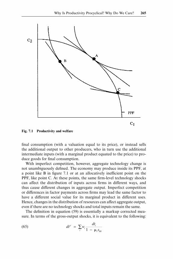
final consumption (with a valuation equal to its price), or instead sellsthe additional output to other producers, who in turn use the additionalintermediate inputs (with a marginal product equated to the price) to pro-duce goods for final consumption.

With imperfect competition, however, aggregate technology change isnot unambiguously defined. The economy may produce inside its PPF, ata point like B in figure 7.1 or at an allocatively inefficient point on thePPF, like point C. At these points, the same firm-level technology shockscan affect the distribution of inputs across firms in different ways, andthus cause different changes in aggregate output. Imperfect competitionor differences in factor payments across firms may lead the same factor tohave a different social value for its marginal product in different uses.Hence, changes in the distribution of resources can affect aggregate output,even if there are no technology shocks and total inputs remain the same.

The definition in equation (59) is essentially a markup corrected mea-sure. In terms of the gross-output shocks, it is equivalent to the following:

( )651

dt wdt

sV

ii

i Mii

=−∑�


Fig. 7.1 Productivity and welfare

This definition correctly measures the increase in aggregate output understandard conditions where an aggregate production function exists. Sup-pose there are no factor market frictions, and that all firms have the sameseparable gross-output production function, always use materials in fixedproportions to gross output, and charge the same markup of price overmarginal cost. Under these assumptions, which are implicit or explicit inmost dynamic general-equilibrium models with imperfect competition,there is a representative producer and an aggregate value-added produc-tion function (see, e.g., Rotemberg and Woodford 1995). In this case, ag-gregate technology change corresponds to our definition dtV.

Qualitatively, the Domar weighted and markup corrected measures turnout to give very similar correlations between technology change and vari-ous business-cycle indicators. (One empirical note of caution is that con-cern the markup corrected measure is sometimes very sensitive to esti-mates of the markup. When we estimate �i for each sector, we hope thatour estimates are unbiased. However, the estimate of value-added technol-ogy change in equation (53), dti /(1 � �i sMi), is convex in �i. Hence, itoverweights sectors where �i exceeds �i, and underweights sectors where�i is less than �i.)

7.3.5 Externalities

So far, we have discussed internal increasing returns but not Mar-shallian externalities. With such external effects, the economy might dis-play aggregate increasing returns even if all firms produce with constantreturns. Hence, one can model increasing returns without having to modelimperfect competition. As a result, models of growth and business cyclesuse such externalities extensively (e.g., Romer 1986; Baxter and King 1991;Benhabib and Farmer 1994). Externalities are almost surely important formodeling economic growth, as suggested by the extensive R&D-spilloverliterature surveyed by Griliches (1992). High-frequency demand spillovers(as discussed in Cooper and John 1988) also seem eminently sensible.However, apart from Diamond (1982), few have proposed models of short-run technological spillovers that operate at high frequencies.

Caballero and Lyons (1992) argued, however, that a basic prediction ofexternality models is a robust feature of the data: Estimated returns toscale should rise at higher levels of aggregation, as the increasing returnsbecome internalized. In other words, aggregate productivity should bemore procyclical than would be implied by estimates of industry-level re-turns to scale. Thus, despite lacking a formal model of short-run externaleffects, they concluded that there is strong prima facie evidence for suchexternalities.

Caballero and Lyons (1990, 1992) proposed an empirical model to esti-mate any short-run externalities. They augmented a firm-level estimatingequation like equation (10) with aggregate inputs as well as firm-level in-


puts. In practice, they used industry-level data on output and inputs, andadded aggregate output to the estimating equation to capture any external-ities that would otherwise be relegated to the error term, dt. They usedNIPA data on real value added by industry. Thus, their basic estimatingequation was essentially

( ) ,66 dv dx dx dti iV

iV V

i= + +� �

where i indexed a two-digit manufacturing industry, and dxV was growthof aggregate capital and labor in manufacturing. (Their 1992 paper alsoincluded various utilization controls.) They found large, positive, and sta-tistically-significant values of � in data from the United States and a num-ber of European countries.

Numerous authors have questioned the interpretation and robustness ofthe Caballero-Lyons’s results. For example, their results may reflect inap-propriate data (Basu and Fernald 1995; Griliches and Klette 1996), incor-rect econometric method (Burnside 1996), or inadequate utilization prox-ies (Sbordone 1997).

Nevertheless, even if one can dismiss their interpretation, the stylizedfact remains that productivity is more procyclical at higher levels of aggre-gation. However, equation (63) suggests an alternative explanation of theCaballero-Lyons stylized fact. Aggregate productivity is more procyclicalbecause the reallocation terms, R, are procyclical. Thus, we can explainthe Caballero-Lyons stylized fact based only on firm-level heterogeneity,without invoking external effects that have questionable theoretical basisin the business cycle context. Indeed, we note that the one well-known eco-nomic model of short-run externalities, Diamond’s (1982) search model,relies on increasing returns to scale in the “matching function” that pro-duces new hires as a function of economy-wide vacancies and unemploy-ment. Efforts to estimate this matching function directly (e.g., Blanchardand Diamond 1990), however, show that it exhibits approximately constantreturns to scale, not large increasing returns. Thus, in the absence of anydirect evidence for short-run externalities, we do not model them explic-itly in this paper.33

7.4 Data and Method

7.4.1 Data

We now construct a measure of “true” aggregate technology change andexplore its properties. As discussed in section 7.1, we estimate technology

33. The search for short-run spillovers remains an active area of ongoing research. See,for example, Bartelsman, Caballero, and Lyons (1994), Cooper and Johri (1997), and Pauland Siegel (1999).


change at a disaggregated level, and then aggregate using the theory insection 7.3. Our aggregate is the private U.S. economy, and our “firms”are thirty-three industries; for manufacturing, these industries correspondroughly to the two-digit Standard Industrial Classification (SIC) level.

Given that each industry includes thousands of firms, it may seem oddto take industries as firms. Unfortunately, no firm-level data sets span theeconomy. In principle, we could focus on a subset of the economy, using,say, the Longitudinal Research Database. However, narrowing the focusrequires sacrificing a macroeconomic perspective, as well as panel lengthand data quality. By focusing on aggregates, our paper complements ex-isting work that uses small subsets of the economy.34

We use data compiled by Dale Jorgenson and Barbara Fraumeni onindustry-level inputs and outputs. These data comprise gross output andinputs of capital, labor, energy, and materials for a panel of thirty-threeprivate industries (including twenty-one manufacturing industries) thatcover the entire U.S. nonfarm private economy. These sectoral accountsseek to provide accounts that are, to the extent possible, consistent withthe economic theory of production. (For a complete description of thedataset, see Jorgenson, Gollop, and Fraumeni 1987.) These data are avail-able from 1947 to 1989; in our empirical work, however, we restrict oursample to 1950 to 1989, since our money shock instrument (described be-low) is not available for previous years.

We weight growth rates (measured as log changes) of capital, labor, andintermediate inputs using the average shares in revenue over the entireperiod. To compute capital’s share, sK, for each industry, we construct aseries for required payments to capital. Following Hall and Jorgenson(1967) and Hall (1990), we estimate the user cost of capital C. For anytype of capital, the required payment is then CPKK, where PKK is the cur-rent-dollar value of the stock of this type of capital. In each sector, we usedata on the current value of the fifty-one types of capital, plus land andinventories, distinguished by the BEA in constructing the national productaccounts. Hence, for each of these fifty-three assets, indexed by s, the usercost of capital is

( ) ( )( )

( ), .67

1

1C r

ITC ds s

s s= +− −

−=�

�

�s 1 to 53

r is the required rate of return on capital, and �s is the depreciation ratefor assets of type s. ITCs is the asset-specific investment tax credit, � is thecorporate tax rate, and ds is the asset-specific present value of depreciationallowances. We follow Hall (1990) in assuming that the real required re-

34. See, for example, Baily et al. (1992), Haltiwanger (1997), Bartelsman and Dhrymes(1998), and Foster, Haltiwanger, and Krizan (this vol.). The aggregation theory in section 7.3implies that our industry data include various intra-industry reallocation terms, includingthe analogous terms to R�, RK, and RL.


turn r equals the dividend yield on the S&P 500. Jorgenson and Yun (1991)provide data on ITCs and ds for each type of capital good. Given requiredpayments to capital, computing sK is straightforward.

As discussed in section 7.1, we require instruments uncorrelated withtechnology change. We use two of the Hall-Ramey instruments: thegrowth rate of the price of oil deflated by the GDP deflator and the growthrate of real government defense spending.35 (We use the contemporaneousvalue and one lag of each instrument.) We also use a version of the instru-ment used by Burnside (1996): quarterly Federal Reserve “policy shocks”from an identified Vector Autoregression. We sum the four quarterly policyshocks in year t � 1 as instruments for year t.36

7.4.2 Estimating Technology Change

To estimate firm-level technology change, we estimate a version of equa-tion (10) for each industry. Although we could estimate these equationsseparately for each industry (and indeed do so as a check on results), someparameters—particularly on the utilization proxies—are then estimatedrather imprecisely. To mitigate this problem, we combine industries intofour groups, estimating equations that restrict the utilization parametersto be constant within industry groups.

As discussed in section 7.2, this estimating equation corresponds to thespecial case where the cost of higher capital utilization is a shift premium.In that case, variations in hours per worker fully captures variations incapital utilization and effort. Thus, for each group we have

( ) .68 dy c dx adh dti i i i i i= + + +�

The markup �i differs by industries within a group (Burnside 1996 arguesfor allowing this variation). The groups are durables manufacturing(eleven industries); nondurables manufacturing (ten); mining and petro-leum extraction (four); and all others, mainly services and utilities (eight).To avoid the transmission problem of correlation between technology

35. We drop the third instrument, the political party of the President, because it appearsto have little relevance in any industry. Burnside (1996) shows that the oil price instrumentis generally quite relevant, and defense spending explains a sizeable fraction of input changesin the durable-goods industries.

36. The qualitative features of the results in section 7.3 appear robust to using differentcombinations and lags of the instruments. On a priori grounds, the set we choose seemspreferable to alternatives—all of the variables have strong grounds for being included. Inaddition, the set we choose has the best overall fit (measured by mean and median F statistic)of the a priori plausible combinations we considered. Of course, Hall, Rudebusch, and Wil-cox (1996) argue that with weak instruments, one does not necessarily want to choose theinstruments that happen to fit best in sample; for example, if the “true” relevance of all theinstruments is equal, the ones that by chance fit best in sample are in fact those withthe largest small sample bias. That case is probably not a major concern here, since the in-strument set we choose fits well for all industry groupings; for example, it is the one we wouldchoose based on a rule of, say, using the instruments that fit best in durables industries asinstruments for nondurables industries, and vice versa.


shocks and input use, we estimate each system using Three-Stage LeastSquares, using the instruments noted above.

After estimating equation (68), we take the sum of the industry-specificconstant ci and residual dtt as our measure of technology change in thegross-output production function. We then insert these industry estimatesin the aggregation equation (63), derived in section 7.3. Note that thisaggregation equation is an accounting identity. It allows us to decomposeaggregate productivity into a technological component plus various non-technological components, including the effects of markups and variousreallocations.

One problem in implementing the decomposition is that we may not, infact, observe period-by-period the appropriate “shadow” factor prices PLi

and PKi defined by equations (25) and (26). We deal with this problem bytaking an explicitly first-order approach to the estimating equation inequation (68), using fixed weights on capital and labor in constructing dxi.(It is straightforward, though it requires some care, to ensure that the ag-gregation equation (63) remains an accounting identity with fixed weights.)This approach is unlikely to lead to major problems in estimating themarkup and materials reallocation terms (R� and RM) in the accountingidentity, since those terms are driven primarily by changes in quantities,rather than changes in the weights (which, in turn, incorporate theshadow prices).

However, the inability to measure prices is a major problem for measur-ing the input reallocation terms (RK and RL), as those terms depend ex-plicitly on differences in prices across sectors. Jorgenson, Gollop, andFraumeni (1987) estimate these terms under the assumption that factorprices are allocative, and that there are zero profits in all sectors (so thatthey can “back out” capital’s input PK as a residual). Although we do notrequire these assumptions elsewhere, we will show summary statistics fromJorgenson and colleagues’ estimates—we emphasize that these are meantto be suggestive only. Since the aggregation equation (63) is an account-ing identity, changing our estimate of one component requires a changein other components as well. We then remove the effect of the input-reallocation terms from the average-markup term (a natural place to takeit from, given appendix equation [A.17]). It is worth emphasizing that evenif we mismeasure the input reallocation terms, this primarily affects ourmeasurement of other nontechnological components of aggregate produc-tivity. In particular, it does not directly affect our estimate of aggregatetechnology, which we built up from disaggregated residuals.

7.5 Results

We now investigate empirically why productivity is procyclical. We seekto identify the importance of (1) imperfect competition, (2) reallocations,


and (3) variable utilization. Controlling for these influences allows us tomove from aggregate productivity to aggregate technology. We then ex-plore the cyclical properties of the “corrected” technology series.

We define aggregate productivity growth as the modified Solow residualdefined in equation (62). This measure differs from the standard Solowresidual since the revenue weights need not sum to one; the differencereflects economic profits or losses. However, we estimate that profits aresmall (about 3 percent on average, using our estimates of required pay-ments to capital), so the results we report are essentially unchanged usingthe standard Solow residual instead.

Table 7.1 reports summary statistics for three series: the Solow residual;a series that makes no utilization corrections, but corrects only for aggre-gation biases; and a “technology” measure based on equation (68), whichuses growth in hours per worker to correct for utilization. The first mea-sure uses aggregate data alone. The other two are based on sectoral Solow-Hall–style regression residuals, as described in the previous section; theseresiduals are then aggregated using equation (63). Hence, aggregate tech-nology change is the weighted sum of sectoral technology changes, as de-scribed in sections 7.1 and 7.3 (see equations [53] and [59]).

Panel A shows results for the entire nonfarm business economy. Ourcorrected series have about the same mean as the Solow residual. However,the variance is substantially smaller: The variance of the fully correctedseries is less than one-third that of the Solow residual, so the standarddeviation (shown in the second column) is only about 55 percent as large.

Table 7.1 Descriptive Statistics for Technology Residuals

StandardMean Deviation Minimum Maximum

A. Private EconomySolow residual 0.011 0.022 �0.044 0.066Technology residual (no

utilization correction) 0.012 0.016 �0.034 0.050Technology residual

(hours corrected) 0.013 0.013 �0.013 0.042

B. ManufacturingSolow residual 0.023 0.035 �0.081 0.080Technology residual (no

utilization correction) 0.014 0.030 �0.085 0.072Technology residual

(hours corrected) 0.018 0.028 �0.030 0.082

Note: Sample period is 1950–89. The Solow residual is calculated using aggregate data alone.The two technology residuals are calculated by aggregating residuals from sectoral regres-sions of gross-output growth on input growth, as described in the text. The “hours corrected”residual corrects for variable utilization by including growth in hours per worker as a separateexplanatory variable, in line with the theory developed in section 7.2.


The reported minimums show that we do estimate negative technicalchange in some periods, but the lower variance of the technology seriesimplies that the probability of negative estimates is much lower. For ex-ample, the Solow residual is negative in twelve out of forty years; the fully-corrected residual is negative in only five out of forty years.

Panel B gives results within manufacturing alone. Data within manufac-turing (especially for output) are often considered more reliable than dataoutside manufacturing. In addition, some other papers (such as Burnside1996) focus only on manufacturing, so these results provide a basis forcomparison. The results are qualitatively similar to those for the aggre-gate economy.

Some simple plots and correlations summarize the comovement in ourdata: Output and inputs are strongly positively correlated, and all are posi-tively correlated with the Solow residual. Figure 7.2 plots business cycledata for the nonfarm private economy: output (value-added) growth dv,primary input growth, dxV, and the Solow residual dp (all series are de-meaned). These series comove positively, quite strongly so in the case ofdp and dv. Table 7.2 shows correlations for these three variables, as well asgrowth of total hours worked (dh � dn). Hours correlate more stronglywith productivity than do total inputs, reflecting the low correlation ofchanges in the capital stock with the business cycle. The 95 percent confi-dence intervals show that all are significant.

Figure 7.3 plots our fully corrected technology series against these threevariables. The top panel shows that technology fluctuates much less than


Fig. 7.2 Aggregate Solow residual, input growth, and output growthNote: All series are demeaned. Sample period is 1950–89. Data is from Jorgenson, Gollop,and Fraumeni (1987). Inputs are a share weighted average of capital and labor growth.

the Solow residual, consistent with intuition that nontechnological factors,such as variable input utilization, increase the volatility of the Solow resid-ual. In addition, some periods show a phase shift: The Solow residuallags technology change by one to two years. This phase shift reflects theutilization correction. In our estimates, technology improvements are asso-ciated with low levels of utilization, thereby reducing the Solow residualrelative to the technology series. The phase shift, in particular, appears toreflect primarily movements in hours per worker, which generally increasea year after a technology improvement. In the model from section 7.2,increases in hours per worker imply increases in unobserved effort, whichin turn increase the Solow residual.

The middle panel plots aggregate value-added output growth (dv)against technology. There is no clear contemporaneous comovement be-tween the two series although, again, the series appear to have a phaseshift: Output comoves with technology, lagged one to two years.

Finally, the bottom panel plots the growth rate of primary inputs ofcapital and labor (dxV ) and the same technology series. These two seriesclearly comove negatively over the entire sample period.

Table 7.3 shows the correlations between our technology measures andbusiness cycle variables. Panel A shows results for the aggregate privateeconomy. With full corrections, the correlation of technology with outputis about zero, and the correlations with inputs are strongly negative: �0.42

Table 7.2 Basic Data Correlations

Output Input HoursGrowth Growth Growth Solow

(dv) (dxV ) (dh�dn) Residual

A. Private EconomyOutput growth (dv) 1Input growth (dxV ) 0.78 1

(0.62, 0.88)Hours growth (dh�dn) 0.80 0.91 1

(0.64, 0.89) (0.83, 0.92)Solow residual 0.84 0.33 0.44 1

(0.72, 0.91) (0.02, 0.59) (0.15, 0.66)

B. ManufacturingOutput growth (dv) 1Input growth (dxV ) 0.81 1

(0.66, 0.90)Hours growth (dh�dn) 0.86 0.98 1

(0.75, 0.92) (0.96, 0.99)Solow residual 0.84 0.36 0.46 1

(0.71, 0.91) (0.05, 0.61) (0.17, 0.68)

Notes: 95 percent confidence intervals in parentheses, calculated using Fisher transformation. Sampleperiod is 1950–89.


for total primary inputs, and �0.44 for hours alone. Both correlations arestatistically significantly negative at the 95 percent level.

The correlations with aggregate technology change differ sharply fromthose predicted by the usual RBC model (e.g., Cooley and Prescott 1995).In particular, in calibrated dynamic general equilibrium models with flex-ible prices, technology shocks generally cause a contemporaneous increasein both inputs and output. These kinds of standard, real business cyclemodels explore whether technology shocks lead to comovement thatmatches the stylized facts of business cycles. Given that the central stylizedfact of business cycles is the comovement between inputs and output, iftechnology shocks drive the cycle then almost any sensible calibration im-plies that technology improvements increase inputs and output.


Fig. 7.3 Technology residual, Solow residual, output and input growthNote: The technology series is the hours adjusted aggregate residual, which measures tech-nology change (adjusted for variations in utilization) for the nonfarm business economy.Aggregate inputs are a share weighted average of capital and labor growth. All series aredemeaned. Entries are log changes. Sample period is 1950–89.

Tabl

e7.

3C

orre

lati

ons

ofTe

chno

logy

Res

idua

lsw

ith

Bas

icD

ata

Out

put

Gro

wth

Inpu

tG

row

thH

ours

Gro

wth

Solo

w(d

v)(d

xV

)(d

h�dn

)R

esid

ual

A.P

riva

teE

cono

my

Tec

hnol

ogy

resi

dual

(no

utili

zati

on0.

46�

0.12

�0.

060.

77co

rrec

tion

)(0

.17,

0.68

)(�

0.41

,0.2

1)(�

0.37

,0.2

6)(0

.63,

0.88

)T

echn

olog

yre

sidu

al(h

ours

corr

ecte

d)0.

04�

0.42

�0.

440.

40(�

0.28

,0.3

5)(�

0.65

,�0.

12)

(�0.

66,�

0.14

)(0

.10,

0.64

)

B.M

anuf

actu

ring

Tec

hnol

ogy

resi

dual

(no

utili

zati

on0.

42�

0.14

�0.

040.

79co

rrec

tion

)(0

.12,

0.65

)(�

0.44

,0.1

8)(�

0.35

,0.2

8)(0

.63,

0.89

)T

echn

olog

yre

sidu

al(h

ours

corr

ecte

d)�

0.40

�0.

64�

0.62

�0.

05(�

0.64

,0.1

0)(�

0.80

,�0.

41)

(�0.

78,�

0.38

)(�

0.36

,0.2

7)

Not

es:9

5pe

rcen

tcon

fiden

cein

terv

als

inpa

rent

hese

s,ca

lcul

ated

usin

gF

ishe

rtr

ansf

orm

atio

n.Sa

mpl

epe

riod

is19

50–8

9.T

echn

olog

yre

sidu

als

are

calc

ulat

edby

aggr

egat

ing

resi

dual

sfr

omse

ctor

alre

gres

sion

sof

gros

s-ou

tput

grow

thon

inpu

tgr

owth

,as

desc

ribe

din

the

text

.The

“hou

rsco

rrec

ted”

resi

dual

corr

ects

for

vari

able

utili

zati

onby

incl

udin

ggr

owth

inho

urs

per

wor

ker

asa

sepa

rate

expl

anat

ory

vari

able

.

Basu, Fernald, and Kimball (1999) explore the negative contemporarycomovement between technology and input growth at length. They arguethat this negative comovement is consistent with sticky price models. Forexample, suppose a firm’s technology improves but the firm cannot changeits price. If its demand curve does not change, then it cannot change itssales—but it can produce that same quantity with fewer inputs. Over time,of course, the firm (and economy) adjust to the technology change.

In terms of our accounting identities, what explains the movement awayfrom a strong positive correlation? Figure 7.4 shows the our estimated uti-lization series—aggregated from the implicit utilization series for each in-dustry using the equation for du from equation (59)—and our estimatedreallocation series, both plotted against the Solow residual. Both utiliza-tion and reallocations are procyclical, as shown here by the positive co-movement with the Solow residual. Each contributes about equally to gen-erating the negative correlation. To see this, we first subtracted the


Fig. 7.4 Nontechnological adjustments to the Solow residualNote: Aggregate utilization growth is a weighted average of estimated industry-level utiliza-tion growth (which includes the estimated markup for the industry). Estimated reallocationsare the sum of R� (reallocations of inputs among industries with different markup estimates),RM (reallocations of intermediate inputs), and RK and RL (reallocations of capital and laboramong uses with different factor prices).

estimated utilization change from the Solow residual; the correlation withinputs fell to about zero. Similarly, we then subtracted the estimated reallo-cation terms from the Solow residual; again, the correlation with inputsfell to about zero.

It is not surprising that utilization is procyclical. After all, utilization isa form of primary input, and inputs are procyclical. It is less obvious whyreallocations are procyclical, as research at a highly disaggregated level—for example, using firms within a narrowly defined industry—finds thatreallocations tend to be countercyclical.37 Low productivity firms enterand expand disproportionately in booms, and contract or disappear dis-proportionately in recessions. Hence, within narrowly defined industries,reallocations appear to make aggregate productivity less cyclical, notmore. (Because we use much more aggregated data on industries, theseintra-industry reallocations will tend to appear as decreasing returns toscale or—given the close link between returns to scale and markups dis-cussed in equation (5) of section 7.1—markups less than one.)

A different process clearly must be at work across aggregated industries.Table 7.4 presents summary statistics for the components of the realloca-tion terms from equation (61). (As discussed in the previous section, weobtained estimates of the capital and labor reallocation terms from DaleJorgenson and Barbara Fraumeni.) None of these components has a size-able mean, but they do have substantial standard deviations. R� and RM

are the most important components of the reallocation term. For the in-strumented series, these terms have standard deviations of 0.72 and 0.51respectively, compared with a total standard deviation of 1.11 for R. Thesum of RK and RL is much less volatile. R�, in particular, comoves stronglywith inputs, with a correlation of 0.7 with aggregate dx.

Why is R� so important over the cycle? Its variation reflects the fact thathigh-markup sectors tend to be more cyclical than average. Hence, in aboom, high-markup (and hence, high marginal product) firms produce a

37. See, for example, Foster, Haltiwanger, and Krizan, chapter 8 in this volume.

Table 7.4 Reallocation by Component, 1959–89 (instrumental variables estimates)

R R� RM �VRK � �VRL

Mean �0.11 �0.17 0.02 �0.03Standard deviation 1.04 0.71 0.47 0.24Minimum �2.86 �2.05 �1.09 �0.51Maximum 1.36 1.08 0.74 0.64

Notes: Entries are percentage points per year. R is the sum of the components shown in thecolumns to the right. R� is reallocations of inputs among industries with different markupestimates. RM is reallocations of intermediate inputs. RK and RL are reallocations of capitaland labor among uses with different factor prices, as calculated by Jorgenson and Fraumeni.See the text for further details.


disproportionate share of the marginal output. We can see this in figure7.5, which shows estimates of the gross-output markup by industry, plot-ted against the relative cyclicality of the industry.38 (The cyclicality wasestimated by regressing dxV

i � dxV on dxV.) High markup industries tendto be durables manufacturing industries, which also tend to be the mostcyclical. In a simulated DGE model, Basu, Fernald, and Horvath (1996)find that reallocations between durable and non-durable producers pro-vide a significant propagation mechanism for shocks to the economy.

One might ask whether the reallocation effects we have identified repre-sent the important gap between (utilization corrected) productivity andtechnology, or whether the difference between the two is still driven mostlyby the “average markup” effect identified by Hall (1988, 1990). We com-pared our results to what we would have found had we used only the “aver-age” correction, that is, that coming from the presence of the �V � 1)dxV

term. Using the correlations with dxV as a benchmark, we found that thereallocation effects are the more important. For the OLS results, produc-tivity corrected for the average effect would have yielded a correlation withinput growth of 0.18, as opposed to 0.23 for the uncorrected series and0.05 for our estimated technology series. For the section 7.4 results, thecorrelation would have been 0.12, as opposed to �0.13 for the estimatedseries. Thus, our reallocation effects are responsible for at least two-thirds


Fig. 7.5 Markups and cyclicalityNote: The horizontal axis shows the utilization corrected markup estimate by industry. Thevertical axis shows the estimated cyclicality coefficient for the industry, estimated by re-gressing industry growth in primary inputs on aggregate growth in primary inputs.

38. The mean markup in figure 7.5 is less than one. As Basu and Fernald (1997a) discuss,the average of sectoral estimates of gross-output markups is less than one, even though theaverage of value-added markups tends to be slightly greater than one. This primarily reflectsthe difference in weights used to aggregate the two.

of the correction. This result should not be surprising since, as we noted,the recent literature finds small average markups. Our results echo thisfinding: Without any utilization correction, we found �V � 1.12, for thehours-corrected case we found �V � 1.05. The surprising result is that evensuch small average markups are consistent with important differences be-tween aggregate productivity and aggregate technology coming from re-allocations across sectors.

7.6 Implications for Macroeconomics

7.6.1 Productivity as Welfare

Why is aggregate productivity growth interesting? The usual justifica-tion is Solow’s (1957) proof that with constant returns to scale, perfectcompetition, and no frictions, it measures aggregate technology change.But in a world with distortions, is the Solow residual merely mismea-sured technology?

In this section we summarize the argument of Basu and Fernald(1997b), who suggest that the answer is no. They show that productivitygrowth correctly computed from aggregate data (i.e., after eliminating themismeasurement caused by changes in utilization) has a natural welfareinterpretation, whether it also measures technology change. In particular,the modified aggregate Solow residual (dp � dxV ) defined in section 7.3—which reduces to Solow’s residual if there are no economic profits—mea-sures welfare change for a representative consumer. This result holds evenwith imperfect competition in output markets and nonconstant returns toscale in production. Intuitively, growth in aggregate output measures thegrowth in society’s ability to consume. To measure welfare change, wemust then subtract the opportunity cost of the inputs used to produce thisoutput growth. Input prices measure that cost, regardless of whether theyalso reflect marginal products. For example, increasing the stock of capitalrequires foregoing consumption, and the rental price of capital measuresthe consumer’s opportunity cost of providing new capital, just as the wagemeasures the opportunity cost of providing extra labor. Proving our wel-fare result requires simply that consumers take prices parametrically.Hence, if productivity and technology differ, then it is productivity thatmost closely indexes welfare.

This conclusion is appealing for two reasons. First, it shows that produc-tivity rather than, say, GDP, is the right measure of economic welfare un-der fairly general conditions. Second, it shows that even with distortions,policymakers can compute interesting quantities from aggregate data—wedo not always need to calculate firm-level or aggregate technology change.In the short to medium run, productivity can change for reasons unrelatedto technology change. Thus, even with distortions such as imperfect com-


petition, when the aggregate Solow residual does not in general index tech-nology change, it remains an excellent index of welfare change. Hence, itremains an appropriate target for policy, as well as a convenient indicator.

In section 7.3, we showed that aggregate technology change needs tobe measured using disaggregated—ideally, firm-level—data. So why doaggregate data yield a meaningful measure of welfare change? The welfareproperties of the Solow residual follow from the equality of relative marketprices to the consumer’s marginal rates of substitution (MRS) betweengoods; this includes the equality of the real wage to the MRS betweengoods and leisure. These equalities hold even when market prices do notreflect the economy’s marginal rate of transformation (MRT) between thosegoods. Equivalently, we need only to investigate the expenditure side of theNational Income and Product Accounts (NIPA) identity; we do not needto know the production technology of firms or the competitive structureof industries.

There are two qualifications to our argument. First, the ratio of factorprices may not equal the consumer’s marginal rate of substitution: Taxes,for example, create a wedge between the two, since the wage paid by firmsthen differs from the wage received by households. The welfare interpreta-tion of the residual requires factor prices received by households, but thismodification is straightforward: All prices should be those perceived bythe household. Second and more seriously, the representative-consumerassumption may fail. Consumers may have different marginal utilities ofwealth or, as in standard efficiency-wage models or bargaining models,they may face different prices. In this case, one cannot compute aggregatewelfare change from aggregate statistics alone. However, we do not claimthat our proposed productivity measure is a completely general measureof welfare change, merely that it is one under much more general condi-tions than the usual Solow residual. It seems a particularly apt measure inthe context of recent macroeconomic models with a representative con-sumer but with imperfect competition in product markets (e.g., Rotembergand Woodford 1992, 1995), or with multiple sectors and costly factor re-allocation (e.g., Ramey and Shapiro 1998).

Figure 7.1 shows the economic intuition underlying our argument. Sup-pose the economy produces two goods, both of which are consumed (andpossibly also used as intermediate inputs). To keep the graph simple, as-sume that the supplies of capital and labor are fixed. The PPF depicts allfeasible (C1, C2) pairs. An economy without distortions attains the socialoptimum at point A, supported by relative prices P1/P2. Now supposethere are distortions. Then the economy might be at an allocatively ineffi-cient point on the PPF, like point B, or even within the PPF, like point C.As shown in figure 7.1, these outcomes can be supported by price ratiosdifferent from the MRT between C1 and C2.

Note that in all cases the consumer’s budget line shows the economy’s


iso-output line, which aggregates heterogeneous output using marketprices (regardless of whether these prices reflect technological tradeoffs.).39

Thus, in this example welfare increases only if output increases. (This is aspecial case of our general result that welfare increases only if productivityincreases, since in this example dk � dl � 0.) Hulten (1978) shows thatunder Solow’s conditions—perfect competition and constant returns—ag-gregate productivity growth represents both technology improvement andwelfare increase. In terms of figure 7.1, Hulten’s result applies to an econ-omy at point A: Output (productivity) can increase only if the PPF shiftsout at point A, that is, if there is (local) technological improvement.

However, the same is not true at points B and C: Output (productivity)can increase without any change in technology, as long as distortions lessen.But these productivity improvements raise welfare, since output and inputsare weighted using prices that reflect the consumer’s MRS between goods.Thus, Basu and Fernald’s (1997b) finding generalizes Hulten’s (1978) resultto the case of imperfect competition and nonconstant returns, and clarifiesthe essence of his argument linking productivity and welfare.

7.6.2 Reallocations as Propagation Mechanisms

It is reasonable for practical macroeconomists to ask when and howthey can avoid the perils posed by the nonexistence of an aggregate pro-duction function (even to a first-order approximation). It is also reasonableto ask whether the reallocation effects that lead to aggregation failurescan also serve a positive function, by providing new amplification andpropagation mechanisms in macro models. In this section we take a firstpass at these large and difficult questions. Much of our intuition comesfrom the extended example of Basu and Fernald (1997a, section 5).

When can we ignore heterogeneity in production and act as if a repre-sentative firm produces all output? Doing so means modeling the produc-tion side of the economy using an aggregate production function for GDP.We ask three questions. First, is this procedure ever sensible if the worldactually has significant heterogeneity? Second, what parameters shouldone use to calibrate the assumed aggregate production function? In partic-ular, can one use estimates from aggregate data and ignore heterogeneity?Third, will the model with heterogeneity reproduce some of the interestingmacroeconomic properties of the single-firm model it replaces?

We emphasize that in this subsection, as in the previous one, we abstractfrom variations in utilization. Capacity utilization is an important empiri-cal issue, because it implies that certain inputs are unobserved by theeconometrician. From the standpoint of theory, however, the possibility ofchanging utilization just changes the calibration of a model by changing

39. For a proof, differentiate the consumer’s budget constraint holding income and pricesfixed.


elasticities of supply and demand, but is not a qualitatively new effect.(For example, variable effort implies that the correct labor supply elasticityis larger than the usual data suggest; variable capital utilization impliesthat the labor demand curve is flatter than the standard production func-tion would indicate.) In this section, by contrast, we ask whether realloca-tions of inputs constitute a qualitatively new propagation mechanism.

We now discuss whether a representative-firm model can capture theimportant features of a world where firms have approximately constant re-turns to scale, but where there are large reallocation effects. When it comesto fluctuations in output conditional on changes in aggregate inputs, theanswer is often yes. The reason is that in many ways reallocations act likeincreasing returns to scale at a representative firm—in both cases, a onepercent change in aggregate inputs is associated with a greater than onepercent change in output. The major difference is that in the representa-tive-firm economy, the degree of returns to scale is a structural parameter.In the economy with reallocations, however, the “effective returns toscale” depends on the nature of the reallocations induced by the drivingshocks. Different shocks are likely to induce different degrees and types ofreallocation, leading to variations in the effective returns to scale parame-ter under different circumstances—a classic example of the Lucas (1976)critique. However, this variation may actually prove an advantage undersome circumstances. To the extent that the economy responds differently toshocks of different types, variable reallocation effects may help explain why.Basu, Fernald, and Horvath (1996) address this question, among others.

This answer to the first question that we posed at the beginning of thissubsection also partially answers the second, on the issue of calibration.We believe that if any single summary statistic is useful, it is likely to bethe degree of returns to scale (or markups) estimated from aggregate datawithout composition corrections. If the Lucas critique problem is not toosevere, this parameter will correctly capture the procyclical behavior ofaggregate output and productivity, but a one-sector model calibrated withthe average of the firm-level parameters would be unable to replicate thisbehavior. But, as the discussion above indicated, a one-sector model cannever be a perfect substitute for a multi-sector model if one wishes tounderstand the response to multiple shocks.

The final question—whether the model with heterogeneity reproducessome of the interesting macroeconomic properties of the single-firmmodel—is the hardest to answer. Indeed, the example of Basu and Fernald(1997a) shows that there are no general answers. Here we discuss one ofmany interesting issues, the possibility of positive-feedback loops thatmight magnify the effects of shocks, and in the limit give rise to multipleequilibria. The work on real rigidities (Ball and Romer 1990) and “indeter-minacy” (e.g., Farmer and Guo 1994) has drawn attention to the impor-tance of positive feedback as a propagation mechanism. Farmer and Guoshow that a very strong form of increasing returns—increasing marginal


product of inputs—provides such positive feedback. The intuition issimple. Suppose the labor demand curve is upward-sloping (due to in-creasing marginal product of labor) and steeper than the labor supplycurve. Also suppose a shock increases lifetime wealth, causing workers tosupply less labor at each real wage (without affecting labor demand). Thisleftward shift in the labor supply curve causes equilibrium labor supply toincrease rather than decrease, as standard neoclassical theory predicts. Ifthis effect is sufficiently strong, the increase in labor and output can beself-justifying. Workers expect higher real wages now and in the future,which reduces their marginal utility of wealth, which increases the equi-librium real wage—validating the initial expectation of higher lifetimewealth.40

An interesting question, then, is whether reallocation effects can createsuch positive-feedback loops. Note that positive feedback depends onchanges in marginal factor prices, since these are the prices that are rele-vant for economic decisions (saving and labor supply). In fact, increasingreturns in the normal sense is not sufficient to create positive feedback. Aswe discussed in Section I, returns to scale can come from fixed costs, andcan be quite consistent with diminishing marginal products. Thus, we con-jecture that reallocations coming from differences in markups, R�, and thefailure of a value-added production function, RM, will have a positive-feedback effect only if the increasing returns accompanying the markupstake the form of diminishing marginal cost.41

Similar caveats apply to RK and RL. Recall that these terms capturedifferences in shadow prices of the same input across firms. If the variancein shadow prices comes only from adjustment costs, and adjustment costsare paid by the firm, then the differences in marginal product will nottranslate directly to differences in factor prices. (Of course, adjustmentcosts usually have general-equilibrium effects on both prices and quanti-ties.) Again, the reallocations induced by quasi-fixity will typically affectthe dynamics of aggregate output following a shock (as discussed by Ra-mey and Shapiro 1998).

However, if the RK and RL terms come from steady-state differences infactor payments across sectors, matters might be different. (In the case oflabor, for example, these differences might come from efficiency wages orunion wage premia.) If the wage differences are allocative for the firm—that is, if the firm equates the marginal product of labor to the above-market-clearing wage, as in Katz and Summers (1989), instead of the wagepremium reflecting efficient bargaining—then these reallocations can havefeedback effects. Even in this case, however, positive feedback is not guar-

40. In a dynamic model one also needs an increase in capital accumulation to increase therate of return to capital.

41. As discussed in section 7.1, we believe on theoretical and empirical grounds that freeentry eliminates long-run economic profits, forcing markups to approximately equal the de-gree of returns to scale.


anteed, because it is unclear what form of rationing rule supports long-run differences in wages for identical labor—that is, how high-paying jobsare restricted to a subset of workers. Basu and Fernald (1997a, Section V)show that the form of the rationing rule determines whether long-run wagepremia that give rise to a non-zero RL also generate positive feedback.Thus, the implications of reallocation for macroeconomic models are likelyto be quite sensitive to institutional assumptions, including institutionsthat do not directly concern production and firm behavior.

The general point of this discussion is that reallocation effects are notjust a “nuisance term”—they are potentially important propagation mech-anisms for shocks, and in the limit can give rise to multiple equilibria. Thisis an important lesson, as recent empirical estimates (including those weprovide above) suggest that average, firm-level returns to scale are approxi-mately constant. We argue that this finding does not necessarily imply thatone should reject macroeconomic parables in which increasing returns ata representative plant play a central role in explaining economic fluctua-tions. Ascertaining which paradigm provides better macroeconomic in-sights is an important, unresolved question, and the focus of on-going re-search.

7.7 Conclusions

In this paper, we explore the meaning and measurement of productivityin a world with frictions and distortions. In such a world, productivitygrowth might not estimate aggregate technology change. We provide ageneral accounting framework that relates growth in aggregate productiv-ity and aggregate technology. We identify various nontechnological termsthat reflect not only variations in utilization, but also changes in the alloca-tion of factors across uses with different marginal products. Marginalproducts, in turn, can differ because of frictions or distortions in the econ-omy. These reallocations affect aggregate output and productivity, withoutnecessarily reflecting technology. Hence, computing aggregate technologychange requires micro data.

The nontechnological components should not necessarily be considered“mismeasurement.” Variable input utilization clearly constitutes mismea-surement, but reallocations do not. In fact, we argue in section 7.6 thateven with distortions such as imperfect competition, a modified Solow re-sidual appropriately measures welfare change. Thus, though much of therecent productivity literature emphasizes the use of micro data, in somecircumstances welfare measurement requires only readily-available na-tional income accounts data.42

Several existing studies provide models of fluctuations in economies that


42. In practice, of course, welfare depends on a broader measure of output than justGDP—for example, household production, investment in human capital, and changes inenvironmental policy. Unfortunately, these items are hard to measure.

deviate in a variety of ways from the standard one-sector model of produc-tion. In those models, the nontechnological sources of productivity fluc-tuations are not always clear, nor is the relationship to other models. Ourgeneral framework can aid in understanding and interpreting the fluctua-tions arising, for example, from sector-specific technology shocks, vintagecapital effects, or imperfect competition with heterogeneity (see, respec-tively, Phelan and Trejos 1996, Gilchrist and Williams 1996, and Basu,Fernald, and Horvath 1996).

Applying our decomposition to the data raises several practical andmethodological issues. We discuss the pros and cons of estimating first-and second-order approximations to the production function, and advo-cate an explicitly first-order approach. We use a model of a dynamicallycost-minimizing firm to derive a proxy for unobserved variations in laboreffort and the workweek of capital. We estimate aggregate technologychange by aggregating industry-level shocks that are “purged” of the ef-fects of variable utilization and imperfect competition.

Variable utilization and cyclical reallocations appear to explain muchof the cyclicality of aggregate productivity. We find that in the short run,technology improvements significantly reduce input use while appearingto reduce output slightly as well. These results are inconsistent with stan-dard parameterizations of RBC models, which imply that technology im-provements raise input use at all horizons. However, Basu, Fernald, andKimball (1999) argue that they are consistent with standard sticky-pricemodels.

Finally, we discuss implications for macroeconomics. We conclude thatreallocations are welfare-relevant, and hence not biases. We also concludethat while accounting for reallocation reduces the average markup and theaverage degree of returns to scale, an economy with strong reallocationeffects can sometimes display the same behavior as an economy with largeincreasing returns. Hence, reallocations constitute a potentially-importantpropagation mechanism, which can be utilized in multi-sector dynamicmodels of business cycles.

Appendix

Derivations from Section 7.3

This appendix presents detailed derivations of the equations in section 7.3.We first derive the relationship between firm-level gross output and firm-level value added, and discuss the interpretation of the value-added equa-tion. We then aggregate firm-level value-added growth to obtain aggregateoutput growth as a function of aggregate inputs, technology, utilization,and reallocations of resources.


As discussed in Section III, the Divisia definition of value-addedgrowth is:43

( ( ).A.1) dvdy s dm

sdy

s

sdm dyi

i Mi i

Mii

Mi

Mii i=

−−

= −−

−

1 1

We now want to substitute in for output growth dyi. In section 7.1, weobtained the following equation for output growth

dy dx s du dti i i i Mi i i= + − +� � ( ) .1

Inserting this equation using the definition of input growth dxi gives

( ) [ ( ) ] ( ) .A.2 dy s dk s dn dh s dm s du dti i Ki i Li i i Mi i i Mi i i= + + + + − +� � 1

We can rewrite this equation as

( ( )( ) ( )

( )

( )( ) ,

A.3) dy ss

sdl

s

Sdk

s du s dm dt

s dx du s dm dt

i i MiLi

Mii

Ki

Mii

i Mi i i Mi i i

i Mi iV

i i Mi i i

= −−

+−

+ − + +

= − + + +

�

� �

� �

11 1

1

1

where primary-input growth, dxVi , is defined analogously to aggregate pri-

mary input growth

dxs

sdk

s

sdl s dk s dli

V Ki

Mii

Li

Mii Ki

Vi Li

Vi=

−+

−≡ +

1 1.

Note that sVKi and sV

Li are shares of capital and labor costs in nominalvalue added.

Now subtract �i sMidyi from both sides of equation (A.3) and dividethrough by (1 � �i sMi). This gives

dys

sdx du

s

sdm dy

dt

s

ii Mi

i MiiV

i

i Mi

i Mii i

i

i Mi

=−

−

+ +

−

− +

−

�

�

�

� �

( )( )

( ) .

1

1

1 1


43. Double-deflation is an alternative method, where V � Y � M, where Y and M arevalued at base-year prices. By differentiating the double-deflated index, we can express thegrowth in double-deflated value added in a form completely parallel to equation (7A.1)—theonly difference is that the intermediate share is calculated using base-year prices, rather thancurrent prices. An implication of this difference is that just as substitution bias affects Las-peyres indices of aggregate expenditure, substitution bias affects double-deflated valueadded. Hence, as Basu and Fernald (1995, appendix) show, double-deflated value addedsuffers all of the biases we identify in this section for Divisia value-added, plus an additionalsubstitution bias.

We can write this equation as

( ( ) ( ) ,A.4) dy dx dus

sdm dy dti i

ViV

i iV Mi

Mii i i

V= + +−

− +� �1

where

(A.5) � ��

iV

iMi

i Mi

s

s≡

−−

1

1

( .A.6) dtdt

siV i

i Mi

≡−1 �

Equation (A.4) relates gross output growth to growth rates of primaryinputs dxV

i , utilization dui, the intermediates-output ratio dmi � dyi, andtechnology. Growth in primary inputs and utilization are multiplied by a“value-added markup” �V

i , defined by equation (A.5). We provide an eco-nomic interpretation of �V

i below.We can now substitute for dyi from equation (A.4) into the definition of

value-added growth (equation [A.1])

( ( ) ( ) .A.7) dv dxs

sdm dy du dti i

ViV

iV Mi

Mii i i

Vi i

V= + −−

− + +� � �1

1

The firm’s revenue-weighted value-added productivity residual, dpi,equals dvi � dxV

i . Hence,

( ( ) ( )

( ) .

A.8) dp dxs

s

dm dy du dt

i iV

iV

iV Mi

Mi

i i iV

i i

= − + −−

− + +

� �

�

1 11

It is obvious from equations (A.7) and (A.8) that value-added growth isnot, in general, simply a function of primary inputs dxV

i . A long literaturein the 1970s (e.g., Bruno 1978) explored whether a “value-added function”exists, and argued that the answer depends on separability properties ofthe production function. The equation above shows that with imperfectcompetition, taking value added to be a function only of primary inputsis generally misspecified—regardless of whether the production functionis separable between value added and intermediate inputs. Separability isa second-order property of a production function, so its presence or ab-sence does not affect first-order approximations like equation (A.7). How-ever, the fact that the output elasticity of materials is �i sMi instead ofsimply sMi is of first-order importance.

Nevertheless, it will be useful to make that further assumption of sepa-rability in order to provide a simple interpretation of value-added growth.In particular, suppose the production function is separable, as follows


( ( ˜ , , , ) [ ( ˜ , , ), ( )].A.9) Y F K L M T G V K L T H Mii

i i i iV i Pi

i i iV i

i= =

The firm combines primary inputs to produce “productive value added,”VPi, which it then combines with intermediate inputs to produce gross out-put. (Note that VPi does not necessarily correspond to the national-accounting measure of value added—that is, the sum of firm-level produc-tive value added need not equal national expenditure.) We can break thecost-minimization problem into two stages: First, minimize the cost of us-ing primary inputs to produce any level of VPi; second, minimize the costof using productive value added and intermediate inputs to produce anylevel of gross output.

In the first stage, the logic from equation (15) implies that the “produc-tive” value-added growth, dvP, depends on the revenue-weighted growth inprimary inputs dxV, plus technology shocks (without loss of generality wenormalize to one the elasticity of productive value added VPi with respectto technology)

( .A.10) dv dx dtiP

iV

iV

iV= +�

In the second stage, the firm seeks to minimize the cost of using valueadded and intermediate inputs to produce gross output. The cost in theminimation problem is MCV

i Vi � PMi Mi, where MCVi is the marginal cost

of value added to the firm. The first-order condition is then MCVi � PiGi

V /�i. Analogously to the problem in section 7.1, we can interpret the value-added markup �V

i as the ratio of the price of productive value added tothe marginal cost of producing it: �V

i � PVi /MCV

i . Hence,

( .A.11)G V

GsV

Pii

iV Vi= �

�

Note that sVi equals PVi Vi /PiYi � (PiY � PMiMi)/PiY, which equals (1 �

sMi). However, without knowing more about the shape of the productionfunction (and hence, the slopes of marginal cost of producing VP and Y ),we cannot make any general statements about the magnitude of the value-added markup �V

i .To do so, we make the further substantive assumption that all returns

to scale are in VP, arising perhaps from overhead capital or labor. This re-quires that G be homogeneous of degree one in VP and H, and that H behomogeneous of degree one in M. Under these assumptions, the left-hand-side of equation (A.11) equals (1 � �i sMi). Equation (A.11) then reads

( ( ) ( ).A.12) 1 1− = −��

�i Mi

i

iV Mis s

Rearranging this equation verifies that the value-added markup �Vi is the

same as we defined in equation (A.5). Hence, just as �i creates a wedgebetween an input price and the input’s marginal product in terms of gross


output, �Vi appropriately measures the wedge between the input price and

the marginal product in terms of value added.Note that for macroeconomic modeling, the value-added markup �V is

likely to be the parameter of interest. Rotemberg and Woodford (1995),for example, make this point in a dynamic general-equilibrium model withimperfect competition. In their model, there are no factor-market frictions,all firms have the same separable gross-output production function, alwaysuse materials in fixed proportions to gross output, and charge the samemarkup of price over marginal cost. Under these assumptions (which areimplicit or explicit in most other dynamic general-equilibrium models withimperfect competition), there is a representative producer and an aggre-gate value-added production function. Rotemberg and Woodford showthat the correct aggregate markup corresponds to �V.

One source of economic intuition for �V is that under some circum-stances, it correctly captures “economy-wide” distortions, as small mark-ups at the plant level translate into larger efficiency losses for the economyoverall. Suppose, for example, that final output is produced at the end ofan infinite number of stages. At each stage a representative firm withmarkup � uses all the output of the previous stage as intermediate input,and also uses primary inputs of capital and labor. Then the percent changein national income—the output of the last (nth) stage—is

dy s dx s dy

s dx s s dx s dy

n M nV

M n

M nV

M M nV

M n

= − +

= − + − +−

− −

� �

� � � �

( )

( ) ( ) ( ) .

1

1 1

1

12

2

We can substitute into this equation for dyn�j, and let j go to infinity. Sinceeach firm is identical, dxV

i is the same for all i as for the aggregate. Thisgives an infinite sum

( ( ) ( )

( ) .

A.13) dy dv s dx s

s dxs

dx

n MV

Mj

j

MV

M

V V

≡ = −

= −−

=

=

∞

∑� �

��

�

1

11

1

1

Thus, �V is plausibly the appropriate concept for calibrating the markupcharged by the representative firm in a one-sector macroeconomic model.

Thus, �V correctly captures the idea that small deviations from perfectcompetition “cascade” in going from gross output to value added, becauseof the “markup on markup” phenomenon: Firms buy intermediate goodsfrom other firms at a markup, add value, and again price the resultinggood with a markup, generally selling some of it to another firm to use asan intermediate good. Nevertheless, this derivation shows that there is alimit to how much the effects can cascade or build up.

Even if we want this value-added markup, however, we still in generalrequire data on intermediate inputs. The reason is that we do not observe


VPi directly, but must infer it from observable gross output and intermedi-ate inputs.

Returning to equation (A.7), real value-added growth depends on pri-mary input growth, changes in the materials-to-output ratio, variations inutilization of capital and labor, and technology. The first term shows thatprimary inputs are multiplied by the value-added markup. The secondterm reflects the extent to which the standard measure of value addeddiffers from “productive” value added VPi, and hence does not properlymeasure the productive contribution of intermediate inputs. Intuitively,the standard measure of value added subtracts off intermediate inputgrowth using revenue shares, whereas with imperfect competition theproductive contribution of these inputs exceeds the revenue share bythe markup. The third term shows that variations in utilization are alsomultiplied by the value-added markup. The fourth term is the value-added-augmenting technology shock.

We now aggregate over firms to get aggregate output growth as a func-tion of technology, aggregate primary inputs growth, and the distributionof inputs. As in section 7.3, we define aggregate output growth dv as ashare-weighted average of firm-level value-added growth

dv wdvii

N

==∑

1

,

where wi � PVi V/PVV. Substituting in from equation (A.7) for dvi gives

( ( ) ( )

.

A.14) dv w dx ws

sdm dy

w du w dt

i iV

iV

i

N

i iV

i

NMi

Mii i

i iV

i i iV

i

N

i

N

= + −−

−

+ +

= =

==

∑ ∑

∑∑

� �

�

1 1

11

11

As in the text, we will define

du w du

R ws

sdm dy

dt wdt

i iV

i

N

M i iV

i

NMi

Mii i

Vi i

V

i

N

=

= −−

−

=

=

=

=

∑

∑

∑

�

�

1

1

1

11

( ) ( ),

.

and

Hence, equation (A.14) becomes

(A.15) dv w dx R du dti iV

iV

MV

i

N

= + + +=∑ �

1

We now decompose the first term into the effects of the “average” value-added markup �V, and the distribution of the markup. Rearranging equa-tion (A.15) gives


( ( )

,

A.16) dv w dx w dx R du dt

w dx R R du dt

Vi i

Vi

i

N

iV V

iV

MV

i

N

Vi i

VM

V

i

N

= + − + + +

= + + + +

==

=

∑∑

∑

� � �

� �

11

1

where

R w dxi iV V

iV

i

N

� � �= −=∑ ( ) .

1

At this point, we are almost finished. However, we still need to relate thefirst term on the right-hand side of equation (A.16) to aggregate inputgrowth. As in section 7.3, consider the case where there was only one typeof capital and one type of labor.44 Aggregate labor and capital are arithme-tic sums across firms, so that K � �N

i�1Ki and L � �Ni�1Li. Aggregate pri-

mary input growth is the share-weighted growth in aggregate capital andlabor growth

dx s dk s dlVKV

LV= + .

Using the definitions of sVKi and sV

Li, and differentiating the definitions ofaggregate K and L, we can write this as

dxP K

P V

K

Kdk

P K

P V

L

Ldl

P V

P V

P K

P V

P

Pdk

P V

P V

P L

P V

P

Pdl

V K

V

ii

L

Vi

Ni

ii

N

iV

i

V

Ki i

iV

i

K

Kii

iV

i

Vi

N

i

NLi i

iV

i

L

Lii

= +

= +

= =

==

∑ ∑

∑∑

1 1

11

.

Noting the definitions of wi, sVKi, and sV

Li, we can write this as

(

( )

A.17) dx w sPP

dk w sPP

dl

w s dk s dl w sP P

Pdk

w sP P

Pdl w dx

Vi Ki

V K

Kii

i

N

i LiV L

Lii

i

N

i KiV

i LiV

i i KiV

i

N

i

NKi K

Kii

i LiV

i

NLi L

Lii i i

= +

= + −−

−−

=

= =

==

=

∑ ∑

∑∑

∑

1 1

11

1

VVK L

i

N

R R− −=∑ ,

1

where


44. In general, suppose there are N firms, NL types of labor, and NK types of capital. Foreach type of capital Kk and labor Ll, the aggregate is an arithmetic sum across firms, so thatKk � ∑N

i�1 KKi and Ll � ∑N

i�1 Lli. Aggregate capital and labor are then defined as a Divisia

index across these types of capital, so that, for example, aggregate labor growth is dl �∑N

Ll�1 PlLL1/PLLdll, where Pl

L Ll is total labor compensation to labor of type l. The derivationsthat follow extend easily to this general case, except that there is a separate input-reallocationterm for each type of labor and capital. Jorgenson, Gollop, and Fraumeni (1987) derive thisresult explicitly.

R w sP P

Pdk

R w sP P

Pdl

K i KiV

i

NKi K

Kii

L i LiV

i

NLi L

Lii

=−

=−

=

=

∑

∑

1

1

,

,

By substituting equation (A.17) into equation (A.16), we find

(

.

A.18) dv dx du R R R R dt

dx du R dt

V VM

VK

VL

V

V V V

= + + + + + +

= + + +

� � �

�

�

Since aggregate productivity equals dv � dxV, it immediately follows that

( ( ) .A.19) dp dx du R dtV V= − + + +� 1

References

Abbott, Thomas A., Zvi Griliches, and Jerry Hausman. 1998. Short run move-ments in productivity: Market power versus capacity utilization.” In Practicingeconometrics: Essays in method and application, ed. Zvi Griliches, 333–42. Chel-tenham, UK: Elgar.

Baily, Martin N., Charles Hulten, and David Campbell. 1992. Productivity dynam-ics in manufacturing plants. Brookings Papers on Economic Activity (Microeco-nomics), issue no. 1:187–267.

Ball, Laurence, and David Romer. 1990. Real rigidities and the non-neutrality ofmoney. Review of Economic Studies 57:183–203.

Barro, Robert J., and Robert G. King. 1984. Time-separable preferences and inter-temporal substitution models of business cycles. Quarterly Journal of Economics99 (November): 817–39.

Bartelsman, Eric J., Ricardo J. Caballero, and Richard K. Lyons. 1994. Customer-and supplier-driven externalities. American Economic Review 84 (4): 1075–84.

Bartelsman, Eric J., and Phoebus Dhrymes. 1998. Productivity dynamics: U.S.manufacturing plants, 1972–1986. Journal of Productivity Analysis 9 (1): 5–34.

Basu, Susanto. 1995. Intermediate goods and business cycles: Implications for pro-ductivity and welfare. American Economic Review 85 (June): 512–31.

———. 1996. Cyclical productivity: Increasing returns or cyclical utilization?Quarterly Journal of Economics 111 (August): 719–51.

Basu, Susanto, and John G. Fernald. 1995. Are apparent productive spillovers afigment of specification error? Journal of Monetary Economics 36 (December):165–88.

———. 1997a. Returns to scale in U.S. manufacturing: Estimates and implica-tions. Journal of Political Economy 105 (April): 249–83.

———. 1997b. Aggregate productivity and aggregate technology. International Fi-nance Discussion Paper no. 593. Federal Reserve System, Board of Governors.

Basu, Susanto, John G. Fernald, and Michael T. K. Horvath. 1996. Aggregate pro-duction function failures. Manuscript.

Basu, Susanto, John G. Fernald, and Miles S. Kimball. 1999. Are technology im-provements contractionary? Manuscript.


Basu, Susanto, and Miles S. Kimball. 1997. Cyclical productivity with unobservedinput variation. NBER Working Paper no. 5915. Cambridge, Mass.: NationalBureau of Economic Research, February.

Baxter, Marianne, and Robert King. 1991. Productive externalities and businesscycles. Discussion Paper no. 53. Federal Reserve Bank of Minneapolis, Institutefor Empirical Macroeconomics.

Beaudry, Paul, and Michael Devereux. 1994. Monopolistic competition, price set-ting, and the effects of real and nominal shocks. Boston University, Departmentof Economics, Manuscript.

Beaulieu, John J., and Joseph Mattey. 1998. The workweek of capital and capital uti-lization in manufacturing. Journal of Productivity Analysis 10 (October): 199–223.

Benhabib, Jess, and Roger E. A. Farmer. 1994. Indeterminacy and increasing re-turns. Journal of Economic Theory 63 (1): 19–41.

Berman, Eli, John Bound, and Zvi Griliches. 1994. Changes in the demand forskilled labor within U.S. manufacturing: Evidence from the annual survey ofmanufactures. Quarterly Journal of Economics 109 (2): 367–97.

Berndt, Ernst R. 1991. The practice of econometrics: Classic and contemporary.Reading, Mass.: Addison Wesley.

Berndt, Ernst R., and Melvin A. Fuss. 1986. Productivity measurement with ad-justments for variations in capacity utilization and other forms of temporaryequilibrium. Journal of Econometrics 33 (October/November): 7–29.

Bils, Mark. 1987. The cyclical behavior of marginal cost and price. American Eco-nomic Review 77:838–55.

Bils, Mark, and Jang-Ok Cho. 1994. Cyclical factor utilization. Journal of Mone-tary Economics 33:319–54.

Blanchard, Olivier J., and Peter Diamond. 1990. The aggregate matching function.In Growth/productivity/unemployment: Essays to celebrate Bob Solow’s birthday,ed. Peter Diamond, 159–201. Cambridge, Mass.: MIT Press.

Bruno, Michael. 1978. Duality, intermediate inputs, and value added. In Produc-tion economics: A dual approach to theory and applications, vol. 2, 3–16. ed. Mel-vyn Fuss and Daniel McFadden. Amsterdam: North-Holland.

Burnside, Craig. 1996. What do production function regressions tell us about in-creasing returns to scale and externalities? Journal of Monetary Economics 37(April): 177–201.

Burnside, Craig, and Martin Eichenbaum. 1996. Factor-hoarding and the propa-gation of business-cycle shocks. American Economic Review 86:1154–74.

Burnside, Craig, Martin Eichenbaum, and Sergio Rebelo. 1995. Capital utilizationand returns to scale. In NBER Macroeconomics Annual 1995, ed. Ben S. Ber-nanke and Julio J. Rotemberg, 67–110. Cambridge, Mass.: MIT Press.

Caballero, Ricardo J., and Richard K. Lyons. 1989. The role of external economiesin U.S. manufacturing. NBER Working Paper no. 3033. Cambridge, Mass.: Na-tional Bureau of Economic Research.

———. 1990. Internal and external economies in European industries. EuropeanEconomic Review 34:805–30.

———. 1992. External effects in U.S. procyclical productivity. Journal of MonetaryEconomics 29:209–26.

Carlton, Dennis W. 1983. Equilibrium fluctuations when price and delivery lagclear the market. Bell Journal of Economics 14 (2): 562–72.

Chambers, Robert G. 1988. Applied production analysis: A dual approach. Cam-bridge: Cambridge University Press.

Cooley, Thomas F., and Edward C. Prescott. 1995. Economic growth and businesscycles. In Frontiers of business cycle research, ed. Thomas F. Cooley, 1–38.Princeton: Princeton University Press.


Cooper, Russell, and Andrew John. 1988. Coordinating coordination failures inKeynesian models. Quarterly Journal of Economics 103 (3): 441–63.

Cooper, Russell, and Alok Johri. 1997. Dynamic complementarities: A quantita-tive analysis. Journal of Monetary Economics 40 (1): 97–119.

Diamond, Peter A. 1982. Aggregate demand management in search equilibrium.Journal of Political Economy 90:881–94.

Diewert, Erwin. 1976. Exact and superlative index numbers. Journal of Economet-rics 4:115–46.

Domar, Evsey D. 1961. On the measurement of technical change. Economic Jour-nal 71 (December): 710–29.

Dotsey, Michael, Robert King, and Alexander Wolman. 1997. Menu costs, stag-gered price setting, and elastic factor supply. University of Virginia, Departmentof Economics, Manuscript.

Farmer, Robert, and Jang-Ting Guo. 1994. Real business cycles and the animalspirits hypothesis. Journal of Economic Theory 63:42–72.

Flux, A. W. 1913. Gleanings from the Census of Productions report. Journal of theRoyal Statistical Society 76 (6): 557–85.

Gali, Jordi. 1999. Technology, employment, and the business cycle: Do technologyshocks explain aggregate fluctuations? American Economic Review 89 (March):249–74.

Gilchrist, Simon, and John Williams. 1996. Investment, capacity, and output: Aputty-clay approach. Finance and Economics Discussion Series no. 1998–44.Federal Reserve System, Board of Governors.

Gordon, Robert J. 1993. Are procyclical productivity fluctuations a figment ofmeasurement error? Northwestern University, Department of Economics, Mim-eograph.

Green, Edward J., and Robert H. Porter. 1984. Noncooperative collusion underimperfect price information. Econometrica 52 (January): 87–100.

Griliches, Zvi. 1992. The search for R&D spillovers. Scandinavian Journal of Eco-nomics 94 (Supplement): 29–47.

Griliches, Zvi, and Tor Jacob Klette. 1996. The inconsistency of common scaleestimators when output prices are unobserved and endogenous. Journal of Ap-plied Econometrics 11 (July/August): 343–61.

Griliches, Zvi, and Jacques Mairesse. 1998. Production functions: The search foridentification. In Practicing econometrics: Essays in method and application, ed.Zvi Griliches, 343–411. Cheltenham, U.K.: Elgar.

Haavelmo, Trygve. 1960. A study in the theory of investment. Chicago: Universityof Chicago Press.

Hall, Alastair R., Glenn D. Rudebusch, and David W. Wilcox. 1996. Judging in-strument relevance in instrumental variables estimation. International EconomicReview 37 (2): 283–98.

Hall, Robert E. 1988. The relation between price and marginal cost in U.S. indus-try. Journal of Political Economy 96 (October): 921–47.

———. 1990. Invariance properties of Solow’s productivity residual. In Growth/productivity/unemployment: Essays to celebrate Bob Solow’s birthday, ed. PeterDiamond. Cambridge, Mass.: MIT Press.

Hall, Robert E., and Dale W. Jorgenson. 1967. Tax policy and investment behavior.American Economic Review 57 (June): 391–414.

Haltiwanger, John C. 1997. Measuring and analyzing aggregate fluctuations: Theimportance of building from microeconomic evidence. Review of the Federal Re-serve Bank of St. Louis (79) (3): 55–77.

Horvath, Michael T. K. 1995. Cyclicality and sectoral linkages: Aggregate fluctu-


ations from independent sectoral shocks. Review of Economic Dynamics 1 (4):781–808.

Hulten, Charles. 1978. Growth accounting with intermediate inputs. Review ofEconomic Studies 45:511–18.

———. 1986. Productivity change, capacity utilization, and the sources of effi-ciency growth. Journal of Econometrics 33 (October/November): 31–50.

Jorgenson, Dale W. 1987. Productivity and postwar U.S. economic growth. Journalof Economic Perspectives 2 (4): 23–42.

Jorgenson, Dale W., Frank Gollop, and Barbara Fraumeni. 1987. Productivity andU.S. economic growth. Cambridge, Mass.: Harvard University Press.

Jorgenson, Dale W., and Zvi Griliches. 1967. The explanation of productivitychange. Review of Economic Studies 34:249–83.

Jorgenson, Dale W., and Kun-Young Yun. 1991. Tax reform and the cost of capital.Oxford: Oxford University Press.

Katz, Lawrence F., and Lawrence H. Summers. 1989. Industry rents: Evidenceand implications. Brookings Papers on Economic Activity (Microeconomics) (1):209–90.

Kimball, Miles S. 1995. The quantitative analytics of the basic neomonetaristmodel. Journal of Money, Credit, and Banking 27 (November): 1241–77.

Lau, Laurence. 1986. Functional forms in econometric model building. In Hand-book of Econometrics, vol. 3, ed. Zvi Griliches and Michael Intriligator, 1515–66.Amsterdam: North-Holland.

Lilien, David M. 1982. Sectoral shifts and cyclical unemployment. Journal of Politi-cal Economy 90 (August): 777–93.

Lucas, Robert E., Jr. 1976. Econometric policy evaluation: A critique. Journal ofMonetary Economics (Suppl. Series): 19–46.

Marschak, Jacob, and William H. Andrews Jr. 1994. Random simultaneous equa-tions and the theory of production. Econometrica 12 (3/4): 143–205.

Morrison, Catherine. 1992a. Markups in U.S. and Japanese manufacturing: Ashort-run econometric analysis. Journal of Business and Economic Statistics 10(1): 51–63.

———. 1992b. Unraveling the productivity growth slowdown in the United States,Canada and Japan: The effects of subequilibrium, scale economies and mark-ups. Review of Economics and Statistics 74 (3): 381–93.

Olley, G. Steven, and Ariel Pakes. 1996. The dynamics of productivity in the tele-communications equipment industry. Econometrica 64:1263–97.

Paul, Catherine J. Morrison, and Donald S. Siegel. 1999. Scale economies andindustry agglomeration externalities: A dynamic cost function approach. Ameri-can Economic Review 89 (1): 273–90.

Phelan, Christopher, and Alberto Trejos. 1996. On the aggregate effects of sectoralreallocation. Journal of Monetary Economics 45 (2): 249–68.

Pindyck, Robert S., and Julio J. Rotemberg. 1983. Dynamic factor demands andthe effects of energy price shocks. American Economic Review 73 (December):1066–79.

Ramey, Valerie A., and Matthew D. Shapiro. 1998. Costly capital reallocation andthe effects of government spending. Carnegie-Rochester Conference Series onPublic Policy 48 (June): 145–94.

Romer, Paul M. 1986. Increasing returns and long-run growth. Journal of PoliticalEconomy 94 (5): 1002–37.

Rotemberg, Julio J., and Garth Saloner. 1986. A supergame-theoretic model ofprice wars during booms. American Economic Review 76 (June): 390–407.

Rotemberg, Julio J., and Michael Woodford. 1992. Oligopolistic pricing and the


effects of aggregate demand on economic activity. Journal of Political Economy100 (December): 1153–07.

———. 1995. Dynamic general equilibrium models with imperfectly competitiveproduct markets. In Frontiers of business cycle research, ed. Thomas F. Cooley,243–93. Princeton: Princeton University Press.

Sato, K. 1976. The meaning and measurement of the real value added index. Re-view of Economics and Statistics 58:434–42.

Sbordone, Argia M. 1997. Interpreting the procyclical productivity of manufactur-ing sectors: External effects or labor hoarding? Journal of Money, Credit, andBanking 29 (1): 26–45.

Schmitt-Grohe, Stephanie. 1997. Comparing four models of aggregate fluctuationsdue to self-fulfilling expectations. Journal of Economic Theory 72 (1): 96–147.

Schor, Juliet B. 1987. Does work intensity respond to macroeconomic variables?Evidence from British manufacturing, 1970–1986. Harvard University Depart-ment of Economics, Manuscript.

Shapiro, Matthew D. 1986. Capital utilization and capital accumulation: Theoryand evidence. Journal of Applied Econometrics 1:211–34.

———. 1996. Macroeconomic implications of variation in the workweek of capi-tal. Brookings Papers on Economic Activity issue no. 2:79–119.

Shea, John. 1997. Instrument relevance in multivariate linear models: A simplemeasure. Review of Economics and Statistics 79 (2): 48–52.

Solon, Gary, Robert Barsky, and Jonathan A. Parker. 1994. Measuring the cycli-cality of real wages: How important is composition bias? Quarterly Journal ofEconomics 109 (February): 1–25.

Solow, Robert M. 1957. Technological change and the aggregate production func-tion. Review of Economics and Statistics 39:312–20.

Varian, Hal. 1984. Microeconomic analysis. New York: W. W. Norton.Weder, Mark. 1997. Animal spirits, technology shocks, and the business cycle.

Journal of Economic Dynamics and Control 24 (2): 273–95.Wen, Yi. 1998. Capacity utilization under increasing returns to scale. Journal of

Economic Theory 81 (July): 7–36.

Comment Catherine J. Morrison Paul

My comments might be entitled, “Where Are the Microfoundations, andDo We Care?” In my view, yes, we do—or at least should—care. We carebecause the questions we are interested in asking, the explanatory powerand interpretability we seek, and the implications for welfare and policywe pursue, all of which are crucial aspects of productivity analysis, arenot effectively addressed or exhibited in the macro-oriented Basu-Fernaldapproach. In addition, it will not surprise anyone who knows of my ownwork over the past twenty years or so that I think this paper in a sense“reinvents the wheel.” The paper raises numerous issues of technological,


Catherine J. Morrison Paul is professor of economics at the University of California,Davis.

market, and cross-market structure that are not novel, but have been ad-dressed in various perspectives in a number of literatures and for a longtime.

However, I must say that the macro literature on which the paper buildshas been critical for both theoretical and conceptual development of pro-ductivity analysis. Also, the issues addressed are indeed important, andthe many literatures in which these issues have been raised are not yet in-tegrated. Perhaps this meeting may be used as a forum in which these dif-ferent types of perspectives may begin to be aired and linked more effec-tively.

The different perspectives building the existing foundations of produc-tivity analysis have been raised in the microproduction theory (parametricand nonparametric), efficiency, macro, “new growth,” and “new IO” litera-tures, most of which have at least some representation in this gathering.The varying perspectives facilitate the creation of additional insights overany one viewpoint, and they are at least starting to converge.

The Basu and Fernald paper is an important case in point because it(implicitly) recognizes the importance of the microproduction theory liter-ature to the macro issues addressed. It at least gives lip service to the basisof the theory of the firm—although the model developed is not really usedfor analysis—and recognizes the usefulness of a “bottom-up” approach.However, rather than building on the existing micro foundation, or synthe-sizing the different perspectives, this treatment primarily sweeps the exist-ing literature under the rug, so rather than working together as the comple-ments they have the potential to be, the different literatures become liketwo ships passing in the night. Perhaps a better analogy, given the conten-tious competition that sometimes rears its head between opposing camps,might be that of the Andrea Doria, where two massive ships crashed inthick fog without seeing each other.

So what is “new” here? Not much, I think. Important seminal work bySolow and later elaborations by Hall are extended to recognize issuesraised already in the macro, as well as the micro, foundations literature.Bringing them together is a useful exercise, but I’m not sure exactly whatwe learn from it. I am left, however, contemplating a number of distinc-tions they make that are useful to think about in the context of the existingmicro foundations literature, and the gap between this and the macro treat-ments. These distinctions will take the form of seven general points I wishto raise.

First-versus Second-Order Analysis

The authors emphasize that their analysis focuses on first-order effects,because that is mainly what is of interest for macroeconomic applications.However, most of the intriguing issues focused on in productivity anal-ysis—including those raised in the paper about utilization, “biases,” scale


effects, externalities, and spillovers—are based fundamentally on second-order relationships.

For example, utilization has to do with over- or underuse of existingstocks of capital and labor (or increases or decreases in the service flow ofthese stocks) by differential use of substitutable and complementary in-puts. This is a second-order phenomenon. Biases in input use (or outputproduction if reallocation among outputs occurs) also have to do withsecond-order effects (although in the macro literature, biases are oftenraised in the context of statistical biases, rather than real biases with re-spect to technology or market valuation stemming from technological andmarket forces). Recognizing these relationships, as in the microproductiontheory literature overviewed by Nadiri and Prucha in this volume, allowsstructural modeling and separate identification of their impacts ratherthan relying on instruments, proxies, and control variables to “back-out”these relationships. Without this, little interpretation of the results is forth-coming.

Top-Down versus Bottom-Up

The authors indicate that macro questions require a top-down perspec-tive but also motivate their analysis via a bottom-up approach, which inthis case means aggregating over two-digit industries.

I have sympathy for the industry-oriented approach, although I wouldhave preferred it to stem from something like the four-digit level, whichrepresents much more homogeneous industry divisions. A true micro (say,plant-level) approach sometimes tends to get lost in the immense heteroge-neity within even the most homogeneous divisions (as is evident from theEllerman, Stoker, and Berndt paper in this volume). Also, typical ques-tions of interest about patterns observed within and across industries re-quire an industry focus for analysis. Thus, beginning with an industry-levelmicro perspective has its merits. Again, though, more structured analysisof the technological and market structure is important. The simple first-order analysis here glosses over the determinants of utilization, scaleeffects, and other technological and market conditions of interest in thesimple average relationships. Once these patterns are determined at theindustry level, bottom-up analysis means to me that they are summarizedacross industries to obtain insights about overall patterns, rather than justlumped into one, or a very limited number of, parameters.

Mismeasurement versus Mismodeling

I am not speaking here of the data mismeasurement issues raised byTriplett and others, which focus on quality. However, one aspect of thequality issue that may be addressed in a more complete microproductiontheory structural model that allows consideration of differential input andoutput patterns is (second-order) changes in input and output com-


position. In this context, for example, changes in the proportion of high-tech capital, or educational attainment levels for labor, as well as trends inoutput mix, may be incorporated.

The main question I am raising about mismeasurement instead has todo with the literature in which the Basu-Fernald piece falls, which refersto mismeasurement in terms of distortions. That is, productivity is consid-ered a combination of technology and distortions. However, much of thetechnological and market structure underlying these distortions, such asutilization and scale patterns, can be identified separately in a micropro-duction theory structural model, which is in fact represented by the theory-of-the-firm model in their paper. This could potentially facilitate the inter-pretation and use of measures of these production characteristics, insteadof collapsing them together as mismeasurement, as is done in the imple-mentation for this macro treatment.

For example, basic micro theory provides us information about the dis-tinction between capital stock and service flow resulting from fixity of thecapital factors and thus fluctuations in the intensity of their use. Therefore,the resulting input use patterns may be evaluated in terms of this concep-tual framework, rather than mismeasurement or a “measure of our igno-rance.” This in turn allows these impacts to be separated from what is leftof the measure of our ignorance, which productivity analysis is designedto illuminate. This relates also to the next distinction.

Primal versus Dual

Although there are some conceptual differences between the (first-order) variable utilization and (second-order) capacity utilization con-cepts, they are inextricably linked. The authors suggest that the first con-cept focuses on the distinction between service flow and stock, and thelatter on valuing the stock. However, in both cases the underlying questionis the service flow. In the first case, it relies on a more primal notion—revising the measure of the capital or labor level to correspond to its ser-vice flow. In the second case it is somewhat more of a nuance. Additionalservices or effort from a given stock of capital (or labor) results from moreintensive application of other inputs, which in turn affects its marginalvaluation in terms of other inputs.

That is, if, given input prices, greater output demand causes more capi-tal effort to be expended, this raises the amount of other inputs applied toproduction from a given amount of capital stock, increasing its marginalvaluation. This revaluation embeds the utilization issue in the dual or priceterm of the price times quantity “total value” of the stock, rather thandirectly in the quantity measure. But the effect is the same: greater utiliza-tion implies a higher capital share. This primal/dual distinction allowsdifferent perspectives on the issue, but they are essentially mirror images.The dual perspective also provides a structure in which shadow values (of


both inputs and outputs), which are alluded to many times in the Basu-Fernald paper, may be measured and analyzed, whereas this is not possiblein the (first-order) primal model.

Technical versus Market Structure

In the Basu-Fernald treatment, the notions of imperfect competitionand scale economies are often used nearly interchangeably. However, ourmicro structure, again learned from principles classes, emphasizes thedifferent motivations and thus interpretations resulting from these produc-tion structure characteristics. Scale economies, which arise from technol-ogy, may be good in the sense of cost efficiency. Effective representationof the cost structure is therefore crucial for appropriate analysis of theseeffects. Market imperfections, which arise from the output demand struc-ture, may be bad in the context of resource allocation. Recognition of themarket structure, and what might be driving evidence of market power,is therefore important for justifiable interpretation and use of “markup”measures. They need to be separately distinguished, identified, and ana-lyzed, which is not possible here.

External versus Internal Effects

Many production and market characteristics mentioned in the produc-tivity literature, raised in this conference, and alluded to in the Basu-Fernald piece may have external or spillover, as well as internal, effects.These include, but are not restricted to, R&D, trade (import penetrationor competition), high-tech capital investment (capital composition), andeducation (labor composition). They also may more generally be character-ized as agglomeration effects. These externalities may generate scale effects,as emphasized by the endogenous growth literature. However, these exter-nal effects may not be disentangled within the simple first-order modelused in the Basu-Fernald paper, and thus again collapse to just anothercomponent of the distortions, mismeasurement, or measure of our igno-rance captured in the residual. Appropriate characterization of these ef-fects must recognize their impact on the cost-output relationship, as exter-nal shift factors. Note also that the notion of the internalization of theseeffects at more macro levels of aggregation has a clear representation inthis context; spillovers that are external at low aggregation levels will beinternal at high levels.

Welfare versus Productivity versus Technical Change

This final distinction is a crucial one in terms of interpretation of mea-sures. Although addressed by Basu and Fernald, I believe it again requiresa microfoundations perspective for appropriate representation, becausethe different types of distortions or components of the productivity growthmeasure independent of technical change may be separately distinguished


in such a framework. For example, returning to the scale economy/marketpower distinction, these different production and market structure charac-teristics have widely varying connotations in terms of welfare analysis andthus policy implications, which thus require separate identification forevaluation of welfare implications.

Therefore, many technological, market, and cross-market issues raised byBasu and Fernald, and in the many linked micro- and macroproductivitystudies in this area, seem to require a more detailed structural microfoun-dations emphasis for effective implementation, interpretation, and use. Thedifferent components of the Solow residual (“measure of our ignorance”)need to be independently captured, identified, and unraveled. There aredisadvantages of a more complex approach to modeling these relationshipsfor more microunits, and ultimately summarizing them across industries toobtain macro implications, because implementation is more complicated.However, such an exercise can provide useful guidance, or at least under-pinnings, for the first-order, top-down macro perspective of these issuesoverviewed in the Basu and Fernald piece. Hopefully, these views or per-spectives are converging. The complementary insights provided by thedifferent approaches should be investigated and synthesized.


why is productivity procyclical? why do we care? · 7 why is productivity procyclical? why do we...

Documents