Working Paper Series Congressional Budget Office

Washington, D.C.

Why Is China’s Saving Rate So High? A Comparative Study of Cross-Country Panel Data

Juann H. Hung Macroeconomic Analysis Division

Congressional Budget Office Email: Juannh@CBO.gov

Rong Qian University of Maryland

Email: Qian@econ.umd.eud

November 2010

Working Paper 2010-07

Working papers in this series are preliminary and are circulated to stimulate discussion and critical comment. These papers are not subject to CBO’s formal review and editing processes. The analysis and conclusions expressed in them are those of the authors and should not be interpreted as those of the Congressional Budget Office. References in publications should be cleared with the authors. Papers in this series can be obtained at www.cbo.gov (select Publications and then Working Papers). The authors thank colleagues in the Congressional Budget Office–especially John Peterson, Bob Dennis, Kim Kowalewski–and participants in the CESifo Workshop at Venice Summer Institute–especially Galina Hale, Menzie Chinn, Bob McCauley, and Ying-Wong Cheung–for helpful comments and suggestions. Priscila Hammett’s valuable research assistance is deeply appreciated.

2

Abstract

This paper uses a large cross-country panel dataset to estimate models of national saving

rates and addresses two related issues. First, to what extent can China’s saving rate be explained

by models of saving rates? Second, what are the factors responsible for China’s extraordinarily

high saving rates?

We find that our benchmark models explain about 72 to 76 percent of China’s national

saving rate during 1990-2007, depending on whether China is included in the dataset. China’s

national saving rate during that period is higher than the predictions of those models by about 10

to 12 percentage points on average. The predominant driver of the explained portion of China’s

high saving rates is China’s relatively low old dependency (the ratio of the population ages 65

and older relative to the population ages 15 to 64). China’s relatively low urbanization, strong

economic growth, and weak social safety net are also important factors. In comparison, the high

degree of currency undervaluation is a smaller contributor to China’s high saving.

3

Why Is China’s Saving Rate So High? A Comparative Study of Cross-Country Panel Data

Juann H. Hung and Rong Qian

1. Introduction

China’s extraordinarily high national saving rate has been at the center of much concern

and analysis in recent years. In March 2005, Chairman Ben Bernanke of the Board of Governors

of the Federal Reserve System proposed that the saving glut (i.e., more saving than needed for

domestic investment) in parts of the world – notably China and some oil-exporting countries –

has contributed to the large US current account deficit and global imbalance. Since then,

concerns about the mounting global imbalance – and more recently, the conviction in some

quarters that the large saving glut was a main culprit of the 2008-2009 financial meltdown and

the accompanying great recession – have drawn even more attention to China’s high saving rate.

China’s saving rate is higher than the average of other high-saving countries, such as its

East Asian neighbors and OPEC countries (Figure 1). Its national saving rate was 54.4 percent

of gross national income in 2007, more than twice of the average saving rate of OECD countries

(Table 1). Moreover, high saving, not weak investment is responsible for China’s large excess

saving. China’s investment/GDP ratio averaged 41 percent from 2000 through 2008, more than

double that in the United States (20 percent) over the same period. However, China’s national

saving rate was even higher: It averaged 48 percent from 2000 to 2008, compared to 15 percent

in the United States.

Many hypotheses have been advanced to make sense of China’s extraordinarily high

saving rate, but it remains unclear to what extent each of those hypothetical factors contributed to

making China’s saving rate higher than most other countries. In particular, whether China’s

4

exchange rate policy has played a significant role in driving its high saving rate has been subject

to much debate. Many analysts have argued that China’s policy of undervaluing its currency is a

major reason for its high saving rate.1 However, other economists have argued that a revaluation

of the yuan would not necessarily eliminate China’s surplus saving because that saving is mainly

rooted in complicated structural factors.2

Indeed, most analysts would agree that saving is driven by various motives,

opportunities, incentives, and constraints. As reported in section 2 of this paper, an extensive

literature has suggested that there are several structural and economic factors that could have

played a part in its high saving for the past two decades: a weak social safety net, an

underdeveloped consumer credit market, a low degree of urbanization, a relatively young

population, and rapid economic growth.3 It may be important to take those factors into account

in any attempt to assess the effect of exchange rate policy – or other types of policies – on

China’s saving.

Against this backdrop, this paper investigates two related empirical questions. First, to

what extent does China’s saving rate exceed the projections of credible models of saving rates?

That is, if we include most traditional and newly formed theoretical determinants (or their

proxies/instruments) of saving rates in a model, how much of China’s saving rate is left

unexplained? Second, what are the factors primarily responsible for China’s extraordinarily high

1 For example, see Wolf (2010) and papers cited in that article. 2 For example, Spence (2010) argues that China’s exchange rate is but one facet in the complexity of its transition toward a middle-income economy, and that revaluing the yuan is unlikely to get rid of China’s surplus saving because China’s high savings are embedded in its overall economic structure – such as the government’s extensive control of income (directly and through ownership of the state-owned enterprises. Similarly, Rodrik (2009) maintains that China’s exchange rate policy is designed mainly as a second-best solution to reduce the distortions and inefficiencies in its economic and financial infrastructure that tend to retard its economic growth. Thus, pressuring China to revalue its currency may do more harm than good. 3 For more detailed discussion of structural and economic factors, see Section 3.1.

5

saving rate? That is, how much of China’s high saving rate is attributable to structural factors, as

opposed to variables that can be significantly influenced by macroeconomic policies in the short

run – such as the exchange rate, the government budget balance, the real interest rate, and

inflation?

Our empirical method consists of two stages. In stage one, we estimate models of

national saving, using a large panel data set of about 70 countries over the time span from 1980

through 2007. In this stage, we are mainly interested in identifying plausible models of national

saving. We consider several explanatory variables, including variables that are traditionally

considered as macroeconomic policy instruments (such as the budget balance, interest rates,

inflation, and the exchange rate) and those that are not (such as real per capital income, income

growth, demography, social safety net, financial development, etc.). Following Loayza,

Schmidt-Hebbel, and Serven (2000), we use a dynamic two-step system generalized method of

moments (GMM) method of estimation. That method has been used by many researchers to

address many issues in the estimation of equations that include lagged dependent variables as

well as explanatory variables that are potentially endogenous.4 On the whole, our coefficient

estimates on the traditional list of variables are not too far off from those of Loayza et al. (2000).

In the second stage, we use our estimated models to make in-sample predictions of

national saving rates for individual countries and to measure the extent to which a country’s

national saving deviates from models’ predictions for that country. Overall, our estimated

models do a very decent job of explaining national saving rates of the 70 countries in the sample.

Thus, they provide a useful benchmark to assess the extent to which China’s saving behavior

4 The GMM estimation was proposed by Chamberlain (1984); Holtz-Eakin, Newey, and Rosen (1988); Arellano and Bond (1991); and Arellano and Bover (1995). It has been applied to cross-country studies by, among others, Easterly, Loayza, and Montiel (1997) and Rodrik (2008).

6

differs from that of the average country and the relative contributions of different explanatory

variables to China’s high saving rate.

We find that China’s lower old dependency (the population ages 65 and older relative to

the population ages 15 to 64) than that of other countries is the most important factor responsible

for China’s higher saving. To a lesser extent, China’s stronger economic growth, weaker social

safety net, and lower urbanization are also important factors responsible for China’s higher

saving rates. China’s currency undervaluation turns out to be a relatively modest contributor to

China’s high saving.5 Other variables either contribute little or have a negative contribution to

China’s saving rate. Overall, China’s national saving rate is higher than the predictions of our

benchmark model by about 10-12 percentage points, depending on whether China is included in

the dataset.

By including the East Asia dummy in some of our models, we find that factors proxied by

that dummy variable also contribute to China’s higher saving rate, and that most of those factors

are those underlying the high-saving, high-growth strategy of East Asian economies. However,

it is beyond the scope of this paper to disentangle the many complex factors that are likely to be

proxied by that dummy.

The remainder of the paper is organized as follows. Section 2 presents existing theories

of China’s high saving rate. Section 3 reports the choice of explanatory variables, empirical

strategy, and the regression results. Section 4 chooses the benchmark model and compares

5 The total effect of China’s currency undervaluation on its saving rate may be higher, since it is likely to have an indirect effect by spurring economic growth (which in turn has a positive effect on the saving rate); however, available estimates suggest that the indirect effect is quite small as well. The estimates in Rodrik (2008) imply that a 10 percent real depreciation of the yuan will increase China’s growth by 0.86 percentage points. This paper’s estimate implies that a one-percentage-point increase in China’s growth will increase China’s saving rate by about 0.2 percentage points, and one percent increase in China’s real per capita GDP will increase its saving rate by about 0.03 percentage points. On average, the yuan’s undervaluation increased 3 percent per year between 2001 and 2007. Both estimates combined imply that the yuan’s undervaluation should increase China’s national saving rate by about 0.06 percentage points per year during that time.

7

China’s national saving rate to the long-term forecast of the benchmark model. Section 5 uses

our estimated models to account for the gap between saving rates of China and the United States.

Section 6 discusses the relationship between China’s high saving and the East Asia model of

economic growth. Section 7 concludes.

2. Related Literature

This paper is related to three strands of economic literature. One strand is concerned with

the causes and consequences of global imbalances – for example, Chinn and Prasad (2003),

Eichengreen (2004), Dooley et al. (2003, 2004), Obstfeld and Rogoff (2005), Roubini and Setser

(2005), Hung and Kim (2006), Congressional Budget Office (2004, 2005, 2007), and Caballero

(2009). Nearly all those papers argue the large global imbalance is not sustainable, though some

are more optimistic than others in how the imbalance will be resolved. Another set of papers

attempts to explain why countries have vastly different saving rates – for example, Edwards

(1996), Masson et al. (1998), Loayza et al (2000), and International Monetary Fund (2005).

Those papers generally use a large multiple-country dataset to estimate the marginal effect of

various structural and nonstructural determinants on national or private saving rates.

More directly related to this paper is the third set of papers, which focuses on addressing

why China’s national saving rate is much higher than the saving rate of most countries – for

example, Modigliani and Cao (2004), Blanchard and Giavazzi (2006), Kuijs (2005, 2006), Aziz

and Cui (2007), Chamon and Prasad (2010), Wei and Zhang (2009), and Wolf (2010). Their

explanations can be roughly summarized as follows:

(1) The Chinese have a higher demand for saving in part because of their frayed social safety

net and an underdeveloped financial sector (Chamon and Prasad, 2010; Blanchard and

8

Giavazzi, 2006; and Kuijs, 2006). The declining public provision of education, health,

and housing services and the lack of pension programs (or, the breaking of “the iron rice

bowl”) creates a strong motive for the Chinese to save. An underdeveloped

banking/financial sector adds to that precautionary demand for saving, because it is

difficult for consumers to borrow from banks to tide them over hard times. China’s small

firms, which generally do not receive the preferential treatment that large state-owned

enterprises do, also tend to retain earnings because they need them to finance their

ventures and to provide a cushion for bad times.

(2) China’s policies favor industry at the cost of jobs and consumer spending (Kuijs, 2006).6

This policy bias has led to higher national saving in two ways. First, it has led household

disposable income to decline relative to national income. Thus, even if the consumption

share of disposable income stays constant, the consumption share of national income will

decline, and the national saving rate increase, as the economy grows.7 Second, those

policies not only have helped to keep corporate profits high; they have also allowed or

encouraged those profits to be retained in the companies (rather than distributed to

shareholders), thereby adding to national saving.8

(3) China has a high rate of economic growth (Modigliani and Cao, 2004). According to the

life-cycle hypothesis, people save when they are wage earners in order to finance their 6 This point is particularly emphasized by Kuijs (2006). Several studies have found that the rapid growth in total factor productivity (TFP) is a main pillar of China’s real GDP growth in the reform era, second only to capital formation. For example, Kuijs and Wang (2006) found that capital accumulation contributed over 50 percent, and TFP growth about 33 percent, to China’s output growth between 1978 and 2004, with employment growth contributing the modest remainder. Bosworth and Collins (2007) also have similar findings. 7 Partly as a result of China’s pro-industry policy, the share of wages and other household income in GDP fell from 72 percent in 1992 to 55 percent in 2007. See Aziz and Cui (2007). 8 See Kuijs (2006). An article in the Economist (October 1st, 2009) with the title “The hamster-wheel” also reports that China’s state-owned enterprises now provide a modest pay-out to the government, but until 2008 they paid nothing at all. In 2008, almost 45 percent of listed companies in China did not pay a dividend.

9

negative saving after they retire. When the economy is growing, workers’ saving will

increase relative to retirees’ dissaving, thereby raising aggregate saving. This channel

may even be stronger for countries such as China where the social safety net is weak for

retirees.

(4) China has an undervalued currency (Goldstein, 2007; Wolf, 2010).9 An undervalued

currency undercuts the abilities of Chinese consumers to purchase foreign goods and

services while it improves the price competitiveness of its exports, thereby keeping

China’s saving rate high.

(5) China has a one-child policy (Wei and Zhang, 2009). The policy, intended to reduce “the

number of mouths to be fed” until the country’s capital stock is large enough to employ

its large pool of excess labor, has increased the male/female ratio in China because of the

tradition of favoring sons over daughters. This in turn has generated a highly competitive

marriage market, driving up China’s saving rates as households with sons are forced to

raise their savings to increase the chance of winning a bride. This theory was proposed

mainly to explain the observation that China’s saving rate started to shoot up around

2002, just as the gender ratio for the marriage-age cohort began to be seriously out of

balance.

This third set of papers suggests that part of the root cause of China’s high saving are the

poverty and underdevelopment of the country and its haste to grow and catch up. Indeed, China

was a destitute country when its pro-market economic reform started in late 1978. Despite its

9 Whether a country’s currency is undervalued depends on the concept used to construct the yardstick (i.e., the fundamental equilibrium exchange rate) used to measure its undervaluation. Those yardsticks include various variations of the Purchasing Power Parity condition, the intertemporal balance of payment equilibrium, and others. Cheung et al. (2007) provides a brief review of some of those concepts and discusses the difficulty in measuring the equilibrium exchange rate and the uncertainty surrounding those measurements. Most analysts have concluded that the Chinese currency has been significantly undervalued.

10

rapid economic growth over the past three decades, China’s real per capital GDP in 2007 was

still lower than one half of an average upper-middle income country’s level and no higher than

an average lower-middle country’s level (Table 1 and Figure 2).10

However, each of those papers tends to focus on a small set of factors alone, and thus is

susceptible to the problems caused by omitted variables. It’s difficult to know a priori whether

each of those factors would still play a significant role in China’s high saving when most of them

are included in the same model, along with other traditionally important variables such as

demography and urbanization. This paper supplements this third strand of literature – by

estimating a model of national saving rates that includes variables from a broad range of theories,

and by using that estimated model to assess the relative contribution of each included variable on

China’s saving rate.

3. Estimating Models of National Saving Rates

We estimate models of national saving, not private saving. This is largely because we are

primarily interested in shedding light on whether the global imbalance can be largely accounted

for by the vast differences in pre-existing economic and institutional conditions among countries.

It is also partly because data on household saving are much more limited than data on national

saving.

3.1 Explanatory Variables

Following Loayza et al. (2000), our specifications are reduced-form linear equations,

drawing upon a broad range of theories for explanatory variables. We include several

10 For example, China’s real GDP per capita was only 38% of that in Mexico (an upper-middle income country) in 2007.

11

“traditional” variables – those that have been included in previous studies – as well as four

“new” variables: an income-adjusted growth rate, the amount of government social spending, the

degree of currency undervaluation, and an East Asia dummy.11

Real income per capita. In a standard Keynesian model, saving is a positive function of

income because people’s ability to save begins to rise after their income exceeds subsistence

level of consumption.12 Lower-income people tend to consume a larger share of their income

than higher-income people. The national saving rate is expected to rise as per capita income rises

within a country or between countries, because most wage earners in poor countries tend not to

have much left to save for retirement after spending on necessities.

Growth of real income per capita. While standard growth models typically posit that an

increase in the saving rate leads to higher economic growth, a growing body of empirical studies

has concluded that the causality from growth to saving is much more robust than that from

saving to growth.13 Theoretical channels for growth-to-saving causality include the life-cycle

hypothesis and the habit-formation hypothesis.14 The life-cycle hypothesis posits that

individuals maximize utility over their lifetime through optimal allocation of their time

resources. Thus, people are dissavers when they are young (before they begin to work or when

their income is too low to cover their expenses) and when they are old and retired; the working

11 Some variables, such as measures of income inequality and degree of financial openness, are not included in our study because of the limited availability of good-quality data across countries over the sample period. 12 This is easily seen if we derive the Keynesian saving equation from a typical Keynesian consumption equation, � � �� � ��, where C is consumption, �� is the subsistence consumption, Y is income, and � is the propensity to consume. The corresponding saving equation would be � � ��� � �1 � ��, implying S/Y = (1�� � ��/�.

Thus, ���/��

�� > 0: the saving/income ratio is a positive function of income.

13 For example, see Bosworth (1993), Carroll and Weil (1994), Edwards (1996), Gavin et al. (1997), Loayza et al. (2000), Attanasio et al. (2000), and Sinha and Sinha (2008). 14 See Modigliani (1970) and Modigliani and Cao (2004) for the life-cycle hypothesis, and Carroll et al (2000) for the habit-formation model.

12

population (those between the young and the old) are those who save. When the economy is

growing, the income and saving of the working population will increase relative to the non-

working population’s income and dissaving, causing aggregate saving to rise. The habit-

formation hypothesis posits that, when the economy is growing, people’s habits tend to pull their

consumption toward the level compatible with their past habits and away from the steady-state

level compatible with the higher level of income. Thus, if an economy receives a shock that

boosts its growth rate, its saving will rise during the transition to the new steady state. The more

powerful are habits, the larger and longer-lived are these transitional effects.

Income-adjusted growth rate. Saving rate may also be a positive function of the growth

rate of real GDP because poor countries have an added incentive to save: to reach the Golden-

Rule steady state by increasing capital accumulation.15 Poor countries that have the motivation

to grow by saving may not be able to do so if they are mired in a poverty trap. However, given a

poor country’s desire to grow and move to a higher income and consumption steady state (i.e.,

the Golden-Rule state), if somehow that country’s growth rate picks up due to lucky exogenous

shocks, that growth rate’s effect on its saving rate may be stronger than that on a richer country’s

rate because of the poorer country’s added incentive to save.16 Because this “catch-up” or

“Golden-Rule” motivation for saving is likely to be positively correlated with the degree of

15 See Phelps (1961, 1965). 16 See Easterly et al. (1997) for stylized facts and empirical findings that suggest shocks are important relative to country characteristics in determining long-run growth. Relatedly, in their attempt to interpret the experience of the East Asian countries in the context of the habit-formation model, Caroll et al. (2000) write “The evidence in William Easterly et al. (1997) suggests that the best way to model the growth experiences in the East Asian countries is as a series of positive shocks. Thus we might interpret the East Asian experience as a sequence of exogenous increases in the ‘broad capital’ embodied in k in our model. . . . . One prediction of our model is that saving rates in the East Asian countries should decline once those economies stop their technological convergence with more advanced economies.” (p. 351)

13

poverty of a country, we enter an income-adjusted growth rate (of real GDP per capita) in the

regression to capture that additional effect of growth on the saving rate.17

Dependency Ratio. The life-cycle hypothesis argues that people are dissavers when they

are young, savers when they are wage-earners, and dissavers again after they have retired. Thus,

a country’s saving declines (rises) when its dependency ratio increases (decreases). We include

both the old dependency ratio (population ages 65 and over/population ages 15 to 64) and the

young dependency ratio (population younger than age 15/population ages 15 to 64) in our

regressions.

Domestic Credit. A greater availability of credit could lead to a decline in saving. The

extent to which individuals can smooth their consumption will depend on their ability to borrow

to finance consumption. If the borrowing constraint is binding, households will be unable to

increase their present consumption even if their expected lifetime income stream has increased,

and they will have to lower consumption in response to negative transitory shocks to income.

Moreover, stringent borrowing constraints mean that households need to save a large sum before

they can think of buying a house or other big-ticket items, and that firms need to rely more on

retained earnings to fund their investment. This paper uses the domestic credits/GDP ratio as an

indicator for the availability of domestic credit. The higher is this ratio, the less stringent is the

borrowing constraint.

Social Safety Net (Government’s Social Spending). An important implication of the life-

cycle framework of saving is that private saving will be affected by the extent and coverage of

the social safety net provided by the government. The more generous the social safety net (such

17 The relative income-adjusted growth rate of real GDP per capita of country i is the product of an income-adjustment factor and the growth rate of real GDP per capita of country i. The income-adjustment factor is the moving average of (Yus/Yi) of the past three years, where Yus is the real GDP per capita of the United States. Thus, the adjusted growth is measured by [moving average of (Yus

t-1,t-3/Yi t-1, t-3)] × [(Yi

t/Yi t-1) -1].

14

as unemployment benefits, medical assistance to the poor, etc.), the less individuals are likely to

save for precautionary purposes. We use government social spending (as a percentage of GDP)

as an indicator of the generosity of the social safety net.

Urbanization (urban population/total population). Rural households, which depend

heavily on agricultural income, tend to save a larger proportion of their income than city

households because precautionary saving tends to be higher for households subject to higher

income volatility. According to this theory, industrial countries that have a higher degree of

urbanization than developing countries will also have a lower saving rate than the latter. In our

view, another likely reason for the negative effect of urbanization on saving rates is related to the

fact that in developing countries dual economy is the norm. Although city dwellers’ living

standards are not far below those of industrial economies, households in many villages still do

not have even most basic services such as running water, electricity, and easy access to buying

goods. In a dual economy, income inequality rises as the economy grows because the rural

population is trapped in poverty. Thus, a rise in urbanization amounts to a decline in income

inequality. Since the saving rate tends to be positively correlated with income inequality – the

richest are the ones that save most – it is likely to be negatively correlated with urbanization.

Real Interest Rate. The effect of a higher real interest rate depends on the relative

strength of substitution and income effects. The substitution effect is positive: An increase in the

real interest rate will increase saving by increasing the rate of return on saving in the current

period relative to that in the next period. The income effect is negative: An increase in the real

interest rate will lower saving because it increases income (an increase in wealth), and thus

consumption, in the current period. In many developing countries, governments are known to

have kept their real interest rates low as a means of financial repression to force the national

15

saving rate to rise – providing cheap credit to industries to promote production while suppressing

consumption through lower interest income.

Inflation. In many developing countries, consumer price inflation means the amount of

consumer goods that wage earners can afford will fall. Inflation thus may increase saving by

redistributing wealth from workers (who tend to have a lower saving rate) toward capital owners

(who tend to have a higher saving rate). Many researchers have also included inflation in a

saving equation as a proxy for macroeconomic uncertainty, an increase of which is expected to

have a positive effect on precautionary saving.18

The Government Budget Balance. In the hypothetical world of Ricardian Equivalence

(RE), change in the government budget balance has no effect on national saving. In that world,

any decrease in the budget balance is completely offset by an increase in private saving because

taxpayers view government spending as a substitute of their own spending and an increase in the

government deficit as an increase in their future tax liabilities. However, most analysts believe

that the taxpayers’ offset is smaller than predicted by the RE hypothesis, and that a decrease in

the budget balance will decrease the national saving rate to some extent.

The Real Exchange Rate. The mercantilist view that a country can boost its net exports –

and thus its national income and national saving – by undervaluing its currency is a long-held

one. Its presumption is that a country, to the extent it succeeds in devaluing its currency and

keeping it undervalued, can boost and preserve the price competitiveness of its tradables. Of

course, that is not a consensus view among economists.19 Nevertheless, the mercantilist view is

18 See Loayza, Schmidt-Hebbel, and Serven (2000). 19 For example, the Harberger-Laursen-Metzler hypothesis postulates that a real devaluation, which causes a decline in real income, will lead to a decrease in savings via the Keynesian channel. See Harberger (1950) and Laursen and Metzler (1950).

16

popular among contemporary commentators in reaction to China’s large trade surplus and high

saving rate.

There is also a growing literature that shows that an undervalued currency has a positive

effect on saving through non-mercantilist channels. For example, Levy-Yeyati and

Sturzzenegger (2007) show that an undervalued currency boosts output growth by increasing

savings and capital accumulation. Korinek and Serven (2010) claim that currency

undervaluation can raise growth through learning-by-doing externalities in the tradable sector

that was otherwise underdeveloped.

We include two exchange-rate variables as explanatory variables: a measure of real

currency depreciation and an index of currency undervaluation.20

East Asia Dummy. It is well known that countries in East Asia – namely, Japan, South

Korea, Taiwan, China, Hong Kong, and Singapore – on average have a higher national saving

rate than do other regions (Table 1). Some analysts attribute this to East Asian’s cultural factors,

while others attribute it to the “East Asian growth model” which includes various policies

designed to promote growth through capital accumulation, by making credit cheaper and more

accessible to industries than to consumers. Because it is difficult to quantify countries’ culture

and growth model, we include an East Asia dummy to capture any marginal effect that “being an

East Asian country” has on the saving rate.

3.2 Data

The main source of data used to estimate the benchmark model is the World Bank’s World

Development Indicators 2009. We also used data from IMF’s International Financial Statistics,

and data from the Asian Development Bank and the United Nations. Appendix 1 reports the

20 The index of currency undervaluation is constructed in the same fashion as that in Rodrik (2008). See Data appendix for the details of its construction.

17

definition and construction of variables and data sources. Appendix 2 shows the range of

variation in the data (Table A1) and the correlation matrix of variables used in our models (Table

A2). After the removal of outliers, we ended up with a sample of 70 countries, from 1980 to

2007. (See Appendix 1 for the criteria used for removing outliers.)

3.3 The Estimation Method

A detailed description of the estimation method used in this paper, and its assumptions

and advantages, is provided in section III of Loayza, Schmidt-Hebbel, and Serven (2000). It is

briefly summarized below.

The empirical analysis is based on generalized method of moments (GMM) estimators

applied to a dynamic system of saving rates. More specifically, GMM is used to estimate a

system of two equations:

(1) ��,� � ���,��� � ����,� � �� � �,�

2� ��,� � ��,��� � ����,��� � ��,���� � ����,� � ��,���� � �,� � �,����

where � is the saving rate, X is a set of explanatory variables, � is the country specific effect and

is the error term. The subscript � represents country and � stands for time period.

This estimation method has several advantages. First, the dynamic specification of

equation (1) allows us to use annual data to estimate both the long-run and short-run effects of

the explanatory variables; thus it is a better way to deal with the presence of inertia in saving

rates than phase-averaging using an arbitrary phase length (such as a five- or ten-year moving

average), which has the disadvantage of distorting the available information. 21 Second, equation

(2) allows us to study the time-series relationship between the saving rate and its determinants by

21 Inertia in saving rates can arise from lagged effects of the explanatory variables on saving, or from consumption habits and from consumption smoothing.

18

eliminating country-specific effects, while equation (1) allows us to study their cross-country

relationship. Finally, the GMM system estimates allow us to control for the potential

endogeneity of the explanatory variables, the possible presence of unobserved country-specific

effects correlated with the regressors, and the problem that the within (fixed-effect) estimates of

� and � are inconsistent in a dynamic specification such as in equation (1).22

The instruments for each explanatory variable that is potentially endogenous in equation

(2) are the lagged levels of that variable, while the instruments in equation (1) are the lagged

differences of that variable.23 These are appropriate instruments under this additional

assumption: there is no correlation between the differences of the right-side variables and the

country-specific effect in equation (1), even if there is correlation between the levels of those

variables and the country-specific effect. With this method, we do not need to assume that the

explanatory variables are strictly exogenous, even though we still need to assume that the

explanatory variables are weakly exogenous – i.e., they can be affected by current and past

realizations of the saving rate but not by future saving rates.

The consistency of the GMM-system estimates depends on whether lagged values of the

explanatory variables are valid instruments in the saving regression. To address this issue, we

perform two specification tests. The first is the Sargan test of overidentifying restrictions first

suggested by Arellano and Bond (1991), which tests the joint validity of the instruments. When

22 When the lagged dependent variable is included as a regressor (to allow the effect of inertia in saving rate), the within estimators of α and are inconsistent. This is because in the within model (the model in which the fixed effects are eliminated by using mean-differenced variables in the regression), the first regressor ( ��,�� � �� , will be correlated with the error ��, � �� ,. Instrumental-variable (IV) estimators using lags as instruments will not solve the problem because any lags of ��, will also be correlated with ��. 23 In equation (2) ���,�� � ��,��� is correlated with ���, � ��,��, yielding inconsistent estimates. To circumvent this problem, Anderson and Hsiao (1981) suggested using ��,��, which is uncorrelated with ���, � ��,��, as an instrument for ���,�� � ��,���.

19

the null hypothesis cannot be rejected, the error term is uncorrelated with the instruments. The

second is the test of the hypothesis that the error term �,� is not serially correlated or, if it is

correlated, that it follows a finite-order moving-average process. First-order serial correlation in

� �,� is expected, even if �,� is serially uncorrelated, because Cov(�,� � �,���, �,��� �

�,���� �0. But � �,� will not be correlated with � �,��� for � � 2, if �,� is serially

uncorrelated. Thus, if the test fails to reject the null hypothesis that Cov(� �,� , � �,��� � � 0 for

� � 2 ��� 3, we conclude that the original error term is serially uncorrelated.

3.4 Regression Results

We report the estimation results in two sets of tables. The first set of tables, Tables 2A

and 2A′, report results of all six specifications that do not include the income-adjusted growth

rate as a regressor, with Table 2A reporting results that include China in the dataset and Table

2A′ reporting those that do not include China in the dataset. The second set of tables, Tables 2B

and 2B′, reports results of all six specifications that include the income-adjusted growth term as

a regressor, with Table 2B reporting results that include China in the sample and Table 2B′

reporting those that do not.

The results of the specification tests shown in all tables generally support the use of

GMM system panel estimates. In all regressions, the Sargan test of overidentifying restrictions

cannot reject the null hypothesis that the instruments are uncorrelated with the error term.

Likewise, the tests of serial correlation reject the hypothesis that the error term is either second-

order or third-order serially correlated, giving additional support to the use of lagged explanatory

variables as instruments in the regression. Thus, in the subsequent discussion, we will interpret

our estimates under the assumption that we have succeeded in isolating the effects of the

exogenous component of the explanatory variables on the saving rate.

20

To facilitate discussion – purely for the purpose of convenience and by no means a

scientific assertion, we will henceforth refer to variables that are conventionally considered as

policy instruments or targets – i.e., the real interest rate, the budget balance, inflation, and the

two exchange rate variables (i.e., change in the exchange rate and undervaluation)– as policy

variables. We will refer to all other explanatory variables, except the dummy variables, as

fundamental variables.

General observations of results presented in all four tables:

• All explanatory variables, except inflation, are statistically significant at the 95%

confidence level in at least two tables. They also all have the expected, or theoretically

justifiable, sign. Explanatory variables’ coefficients in Tables 2B and 2B′ are somewhat

more stable across models than those in Tables 2A and 2A′ . In particular, the coefficient

estimates on both urbanization and social spending in Tables 2A and 2A′ are

considerably more varied in magnitude and statistical significance across models than

those in Tables 2B and 2B′.

• The national saving rate is estimated to be a positive function of (real) per capita GDP,

the growth rate of per capita GDP, the income-adjusted growth rate, the budget balance,

the real exchange rate change (i.e., real currency depreciation), and undervaluation; and

a negative function of domestic credit/GDP, old dependency, young dependency, social

safety net, and urbanization.24 The real interest rate has a negative coefficient,

suggesting that its income effect outweighs the sum of its substitution and wealth effects.

This is not particularly counterintuitive for developing economies in which other motives

24 The real exchange rate is the price of the U.S. dollar in foreign currency terms, adjusted for relative prices. Thus, a higher level of the real exchange rate means the real purchasing power of a country’s currency is lower in dollar terms, and an increase in a country’s real exchange rate means a depreciation of its currency.

21

for saving are likely to outweigh the substitution effect of the real interest rate.25 One-

percentage point increase in government saving leads to about 0.3 percentage points

increase in national saving, suggesting that there is a partial Ricardian Equivalence effect.

• The coefficient estimates on both exchange-rate variables – change in real exchange rate

(i.e., real currency depreciation) and undervaluation – are statistically significant with

similar magnitudes in both Tables 2A and 2A′ and in both Tables 2B and 2B′. This

suggests that the marginal impact of the real exchange rate on saving rates in China is not

markedly different from that in other countries. In each table, the magnitudes of those

exchange-rate coefficients are also stable regardless of whether the East Asia dummy is

included in the regression, suggesting that the net effect of factors captured by that

dummy – be it a culture of thrift, industrial policies, or something else – is largely

independent of the exchange rate.

• The coefficient estimates on the lagged dependent variable are around 0.5 in all four

tables, indicating that there is a high degree of persistence in national saving. This in turn

implies that the long-run effects (on the saving rate) of other explanatory variables are

about twice as large as their respective short-run effects, if all changes in these variables

were permanent.

Comparing Table 2A to Table 2B:

• The coefficient estimate on income-adjusted growth rate is statistically significant, with

an expected sign and a reasonable magnitude, in all six regressions reported in Table 2B.

25 Loayza, et al. (2000) point out that such results should be taken with some caution. In view of the strong negative correlation between inflation and the real interest rate, the real interest rate measure may reflect more the action of nominal interest-rate controls and financial repression than the intertemporal rate of substitution of consumers.

22

This offers some evidence of the “catch-up effect” hypothesis, which argues that the

marginal effect of economic growth on the saving rate tends to be higher for poor

countries with high growth rate than for richer countries.

• All six specifications with the income-adjusted growth rate appear to be better than the

ones without: The coefficient estimates on urbanization and on social spending in

regressions in Table 2B are more statistically significant and lie within a narrower range

than their counterparts in Table 2A.

Comparing Table 2B to Table 2B′:

• On average, the coefficient estimates on income-adjusted growth are somewhat larger in

Table 2B than in Table 2B′. This suggests that the catch-up effect is more powerfully at

work in China than in other countries.

• The coefficient on the East Asia dummy in Table 2B′ (Model B6) is statistically

insignificant and quantitatively much smaller than that in Table 2B (Model B6). Because

the former is estimated without China in the dataset, this result suggests that there are

other factors proxied by the East Asia dummy that are at work in China more powerfully

than in other East Asian economies.

Comparing our results to the literature:

To our knowledge, IMF (2005) is the only study of national saving rate using a large

cross-country panel dataset since Loayza et al. (2000).26 A comparison between coefficient

estimates in Table 2A (the regression closest to those two papers in regression specification and

the construction of explanatory variables) and coefficient estimates in those two previous papers

26 IMF (2005) applies the same methodology as in Loayza, et al. (2000) to a smaller set of explanatory variables.

23

are presented in Table 3. Given that there are considerable differences between our paper and

those papers, it comes as no surprise that there are some differences in the size of the estimates in

the three studies.27 Nevertheless, it is reassuring that our long-term coefficient estimates on the

old dependency ratio, the young dependency ratio, urbanization, the real interest rate, and the

real exchange rate change, are all reasonably close to those in Loayza et al. (2000), and that

those on the growth of real GDP per capita, real GDP per capita, and domestic credit/GDP are

qualitatively comparable to (though noticeably smaller in absolute terms) than those in Loayza et

al. (2000). Our coefficient estimate on the budget balance (0.283) is also close to that in IMF

(2005).

4. Choosing the Benchmark Model to Assess China’s Unexplained Saving

Which of our estimated models is most appropriate as the benchmark model for our

purpose? Since we have already established that models with the income-adjusted growth rate

perform better than those without, let us narrow our comparison to the six models presented in

Tables 2B and 2B′. Unsurprisingly, the extent of each country’s unexplained saving – the

difference between the national saving rate and the long-term forecast of a regression equation –

varies across the six models and depends on whether China is included in the dataset (Table 4).28

By the standard of the average rate of unexplained saving of all OECD countries and that of

China, the best choice is Model B6 – the model that includes the East Asia dummy and the two

27 The differences include those in model specification, measurement of independent and explanatory variables, number of countries and sample period. For example, this paper uses data from 1980 to 2007, and measures national saving as gross national income (GNI) minus consumption. In comparison, Loayza et al. (2000) uses data from 1965 to 1994, and measures national saving as gross national disposable income (which equals to GNI plus all net unrequited transfers from abroad) minus consumption . 28 The long-term model forecasts are obtained by ignoring fixed effects of each country, summing up only the long-term marginal effects of all explanatory variables in each model, where the marginal effect of variable X = (level of variable X)× [coefficient of variable X/(1-coefficient of lagged saving)].

24

exchange rate variables. However, Model B6 should be ruled out because our preceding

analysis found that the East Asia dummy largely reflects China-specific factors – its unique

industrial policy mix, its government’s ability to command those policies through the state-

owned enterprises and other means, or something else. Having ruled out Model B6, the

unambiguous winner is Model B5 as it has the best fit to China’s saving rate and OECD

countries’ average saving rate. Moreover, its ability to fit national saving rates remains relatively

unchanged regardless of whether it is estimated with or without China in the dataset (Figures 3.1

to 3.11). This is another advantage of choosing Model B5 over Model B6: The ability of Model

B6 to fit national saving rates depends on, to a greater degree, whether China is included in the

dataset (Figures 4.1 to 4.6).

Using Model B5 as the benchmark model, China’s average unexplained saving from

1990 to 2007 was about 10.3 percentage points (or, 24% of its national saving rate ) if China is

included in the dataset of estimation, and 12.2 percentage points (or 28% of its national saving

rate) if China is excluded from the dataset. China had a higher level of unexplained saving rate

over its sample period than almost all other countries included in the sample, even though its

average saving rate was actually exceeded by that of three countries – Bhutan, Singapore, and

Brunei (Tables 4.1 and 4.2).

5. What Factors are Responsible for China’s High National Saving Rate?

The preceding analysis suggests that about three-quarters of China’s high saving rate is

attributable to explanatory variables included in the benchmark model (Model B5 in Table 2B).

This section assesses the relative importance of each model variable’s contribution to China’s

high saving rate by estimating its contribution to the saving-rate gap between China and OECD

25

countries. It then discusses the factors outside the model that may have been responsible for the

rise in the unexplained portion of China’s saving rate after 2001.

The contribution of each variable to the China-OECD saving gap depends on the

difference in the magnitude of that variable as well as the elasticity of the saving rate with

respect to that variable. Table 5 shows that the magnitudes of most variables in China are quite

different from those in the OECD economies. The levels of old dependency, social spending, and

urbanization in China are much lower than their average levels in OECD, while the growth rate

(including the income-adjusted growth rate) and the degree of currency undervaluation are much

higher in China than that in OECD. To provide some degree of sensitivity analysis, Table 6.1

presents the contribution of each explanatory variable using coefficient estimates in the

benchmark model as well as those in other models reported in Table 2B.

Table 6.1 shows that, regardless of which model’s coefficient estimates are used, China’s

much lower level of old dependency stands out as the explanatory variable most responsible for

China’s much higher saving rate. The rankings of other factors are somewhat model-dependent.

Based on our benchmark model, the other important factors are China’s higher growth rate of

real GDP per capita (including the adjusted growth), weaker social safety net, and lower

urbanization ratio. The preeminence of old dependency in accounting for the China-OECD

saving gap remains unchanged when we use coefficient estimates without China in the dataset

(Table 6.2). That preeminence stemmed from both the large elasticity of saving in response to

the old dependency ratio and the fact that the ratio is much higher in OECD than in China (by 12

percentage points). The relative modest contribution of China’s currency undervaluation, on the

other hand, mainly reflected the small elasticity of saving in response to currency

undervaluation. The other variables – domestic credit/GDP, the young dependency ratio, and

26

real GDP per capita– made either little or negative contributions to the China-OECD saving

gap. In particular, everything else being equal, the higher income level of the OECD countries

meant China’s saving rate should have been lower than OECD’s rate by 15 percentage points

during 2000-2006. From this perspective, those positive factors together contributed over 27

percentage points to the China-OECD saving rate gap during that period.

All those positive factors’ contributions to the saving gap declined somewhat in recent

years, however. The contribution of China’s lower old dependency ratio declined from 77% in

1990-2000 to 59% in 2001-2006; that of China’s higher growth rate fell from 29% to 19%, that

of its weaker social safety net fell from 27% to 19%; and that of its lower urbanization fell from

26% to 17%. China’s real exchange rate, including both effects of real currency depreciation

and currency undervaluation, turns out to be a more modest contributor to its higher saving rate

than those four factors in both periods: Its contribution was 14% in 1990-2000 and 12% in 2001-

2006.29 Indeed, the benchmark model as a whole has become less able to account for China’s

saving rate in recent years (Figure 3.1). Even Model B6, which includes the East Asia dummy

and tracks China’s saving rate remarkably well before 2001, becomes less able to explain

China’s saving after 2001 (Figure 4.1)

Clearly, some factors not included in our models have become increasingly important in

driving China’s saving rate in recent years. The literature suggests three possibilities.

The first is the possible effect of the 1997-98 Asian crisis on boosting both private and

government precautionary saving. In one of his speeches in 2009, Zhou Xiaochuan, the

governor of the People’s Bank of China, claimed that one factor behind East Asian countries’

high saving rates and large foreign reserves is “defensive reactions against predatory

29 The contribution of China’s lower old dependency ratio is calculated as equal to 14.1/18.4 in 1990-2000, and 13.9/23.6 in 2001-2006. Those of other variables are calculated in the same fashion.

27

speculation” that had led to the Asian financial crisis.30 Park and Shin (2009) also argue that the

Asian crisis has had a positive effect on precautionary saving in East Asian economies, boosting

their current account surpluses. When we added an Asian Crisis dummy to our regressions, we

find that the Asian Crisis dummy indeed has a positive effect on national saving in several

specifications (Tables 2C and 2C′). However, that dummy is not significant in all the

specifications that include the exchange rate variables, suggesting that the exchange rate may be

one important tool used to reach the higher level of precautionary saving in response to the Asian

crisis.

The second possibility is the widening gender imbalance hypothesized by Wei and Zhang

(2009). According to the authors, China’s one-child policy has resulted in a surplus of men. This

in turn has generated a highly competitive marriage market, driving up China’s saving rates as

households with sons were forced to raise their saving to increase the chance of winning a bride.

The authors presented evidence to show that the saving rate started to shoot up around 2002

largely because that was when the gender ratio for the marriage-age cohort began to be seriously

out of balance, enhancing incentives of households with sons to increase saving for the sake of

winning a bride.

The third possible factor is the increase in the transfer of income away from the

household sector to banks and businesses as a result of policymakers’ efforts to resolve the crisis

posed by the surge in non-performing loans (NPLs) that began in the late 1990s. The

government began to implement a variety of measures to reduce the NPLs in 1998; those efforts

began to speed up in earnest in 2001 as the government stepped up the country’s transition from

a centrally planned economy to a market-oriented one.31 According to Pettis (2010), the

30 See Zhou (2009). 31 See Xu (2005).

28

government’s measures to resolve the bad-loan crisis all resulted in passing the bail-out costs on

to bank depositors.32 Thus, he argues, household income share, already a low share of domestic

income by international standards, declined further. It is undeniable that China’s household

income share did begin to decline significantly in 2002, regardless of whether the NPL bailout

was the main cause (Figure 5). That decline, combined with a rising personal saving rate during

the same period (Figure 6), no doubt contributed to the rise in China’s national saving rate

unexplained by our models in recent years.33

6. China’s High Saving and the East Asian Economic Growth Model

The finding that Model B6, which includes the East Asia dummy, explained nearly 92

percent of China’s saving rate from 1990 to 2006 begs this question: How much of China’s high

saving rate is attributable to factors that are shared by East Asian economies but different from

the rest of the world? This section discusses this issue by drawing from empirical findings of

this paper, stylized facts, and the literature.

The fact that the coefficient estimate on the East Asia dummy becomes statistically

insignificant when Model B6 is re-estimated without China in the dataset would seem to suggest

that the dummy mainly captures China-specific factors. However, that the dummy remains

statistically significant in Model A6 – the model that excludes the income-adjusted growth rate –

32 According to Pettis (2010), the government used three tools to reduce non-performing loans. First, the central bank slowed the accumulation of those loans by keeping lending rates low, making it easier for struggling businesses to roll over the debt while the growth of the economy reduced the real value of debt payments. Second, policymakers infused the banks with additional equity, partly directly and partly by purchasing bad loans at above their liquidation value. They financed these capital infusions by borrowing at artificially low rates, thereby passing the repayment burden on to lenders. Finally, the central bank mandated a wide spread between the bank lending and the deposit rate, which helped to recapitalize banks by increasing their profitability. All three tools required that bank depositors subsidize the bail-out of the banking industry. 33 For example, see Aziz and Cui (2007) for discussion of the role of household income in China’s low consumption.

29

whether it is estimated with or without China in the dataset suggests one cannot easily dismiss

the East Asia dummy as merely a proxy for China-specific fixed effects. More plausible is the

interpretation that there is a significant overlap of the factors captured by the East Asia dummy

and those proxied by the income-adjusted growth rate. Thus, when China is excluded from the

dataset, the East Asia dummy becomes insignificant in a model that already includes the adjusted

growth rate, but remains significant in the model that does not. The question is: What are those

common factors captured by both the East Asia dummy and the income-adjusted growth rate?

Volumes have been written about why the East Asian economies have managed to grow

much more rapidly than other developing economies. In that literature, the so-called East Asian

growth model can be loosely described as a “high saving-high investment-high growth” strategy

modeled on Japan’s model of economic growth and development.34 Although the specific policy

mix varies across East Asian economies, that growth model basically relies on heavy government

interventions that favor capital formation (i.e., industrialization) at the expense of consumer

spending, through various means that effectively force savings from consumers to keep the cost

of financing low for investment.35 For example, several East Asian economies – including Japan,

South Korea, and Taiwan – provided affordable credit to business by allowing inflation to

effectively curtail consumer spending in some periods during their years of industrialization.

Until recent years, consumers generally had more difficulty obtaining credit than did business

entities in those countries. Even in Japan, which grew to become a rich and industrialized

34 For example, see Hirono (1988) and other articles collected in Hughes (1988). A study by the World Bank (1993) also emphasizes that a “virtuous circle” – going from higher growth, to higher savings, to even higher growth – has played a central role in successful development experiences in East Asia. 35 Foreign credit tended to be too expensive or too scant during the early stage of industrialization in those countries after WWII. For more discussion of the similarities and differences between China’s development model and those of the East Asian model, see Baek (2005) and Boltho and Weber (2009).

30

country more than three decades ago, policies that favor business investment at the expense of

consumer demand have only begun to fade or be reversed in recent years.36 Haggard (1988)

argues that a key element underlying those East Asian governments’ ability to implement those

policies with success is their political systems “in which economic policymaking process was

relatively insulated from direct political pressures and compromises” and “legislatures are

historically weak or non-existent and other channels of political access and representation tightly

controlled, even under nominally democratic regimes.”

There is plenty of evidence that China has adopted its neighbors’ successful strategies of

achieving rapid growth through high saving and investment. For example, China’s policies are

known to favor capital-intensive investment, which arguably is less effective in creating jobs to

absorb its large pool of excess labor than labor-intensive investment is. Growth has been capital-

intensive and profits have outpaced wage income, a situation that has which depressed household

consumption relative to national income (Figure 5). Capital-intensive production has been

encouraged by low interest rates and by the fact that most state-owned firms do not pay any

dividends, allowing them to reinvest all their profits. Furthermore, the government has also

favored manufacturing over services by policies such as holding down the yuan exchange rate

and suppressing the prices of inputs such as land and energy. Most economists now agree that a

main reason underlying the rise in China’s national saving rate is that households’ disposable

income had grown more slowly relative to GDP, depressing their consumption share of GDP.

Indeed, some authors – for example, Kuijs (2005, 2006) and Ma and Yi (2010) – have pointed

out that a major driver of the sharp rise in China’s national saving rate is the significant rise in

36 Japan’s national saving rate stayed over 30 percent throughout its fast-growing decades. It fell below 30 percent only after 1997 as its government deficit continued to rise during its prolonged economic slump of the previous two decades. Still, despite its large government deficit, Japan’s average national saving rate during 2000-2006 (26.4%) was still higher than that of OECD (23.8%).

31

China’s corporate saving (the sum of retained earnings and depreciation) and government saving

(Figure 7).

Ma and Yi attribute the rise in corporate saving to the combination of two related factors:

(1) a very tough corporate restructuring during 1995-2005 that consequently boosted corporate

efficiency and profitability; and (2) a government policy that state companies were not required

to pay dividends to the government.37 Those two factors, together with the fact that smaller

private firms probably need to fund investment with retained earnings because they tend not to

have easy access bank loans, imply that corporate retained earnings in China rose in tandem with

net corporate profits, which rose from about 4 percent of GNI in 2001 to 10 percent in 2007

(Figure 8).38 The rise in government saving from 2001 to 2007 was even larger than that in

corporate saving (Figure 7). That rise mainly stemmed from the fact that much of the increase in

government revenue went to government investment (which is considered government saving) as

opposed to consumption (such as unemployment benefit, medical care for the poor, etc. Chinese

central government actually ran a small budget deficit during that period, because its total

spending (the sum of investment and consumption) exceeded its total revenue.39 The household

37 The dividend policy allowed the bulk of the dividend payouts by listed Chinese state companies to go to their non-listed parent holding companies (direct majority shareholders) instead of the government (the ultimate owner) and thus is still retained within the corporate sector. 38 Ma and Yi (2010) also argue that depreciation as a share of GDP has probably risen over time because (1) depreciation is positively linked to the higher capital stock and newer vintages of capital, and (2) the capital stock per worker in the industrial sector has at least doubled in the past decade as a result of rapid industrialization. Since there are no official data of depreciation, the authors cite Bai et al (2006), which claimed China’s capital stock as a ratio to GDP rose from 130% to 170% between the early 1990s and the mid-2000s, to support their argument. 39 Ma and Yi (2010) suggest three reasons behind the Chinese government’s decision to invest rather than consume most of its rising income. First, the anticipation of rapid population aging and the 1997 pension reform prompted increased pension contributions by the corporate and household sectors. These contributions are parked under various pension funds administered by the government. These funds have been invested, directly or indirectly, in financial and physical assets at home or abroad. Thus, the rise in government saving may be partly due to the build-up of pension assets. Second, local Chinese government officials have incentives to start new investment projects, as promotions have been mainly based on economic growth in their jurisdictions. Hence they have an innate tendency to invest more rather than to provide additional public services for a given rise of government revenues,

32

saving/GDP ratio, despite the decline in the share of national income going to households, has

again surpassed enterprises saving/GDP after 2004 (Figure 7). In part, this is due to the

continuing rise in household saving rate since the early 1990s, which reached nearly 30 percent

by 2008 (Figure 6).40

Clearly, all three players – the household sector, the corporate sector (both private-owned

and state-owned enterprises), and the government – have been responsible for China’s high

saving rate. This is consistent with what one would expect from a country that has adopted the

East Asian growth model, especially if the first two groups’ high savings are in part induced by

government policies.

The evolution of national saving and economic growth in Japan, the grandfather of the

East Asian growth model, suggests that we are likely to see a slow normalization of China’s

saving rate once the Chinese economy is better developed and ranked among rich countries (in

terms of real GDP per capita). Given that China’s real GDP per capita in 2007 was still slightly

below that of Japan in the early 1960s, however, it is unlikely that China’s saving will decline to

a more “normal” level within the next decade.41 Nevertheless, there are signs that that process of

“normalization” has begun. For example, the government allowed its currency to fall against the

US dollar by over 17 percent from June 2005 to July 2008 (the beginning of the 2008-2009

global financial turmoil). That trend is likely to continue once the global economy begins to

thereby boosting government saving. Third, while a rising share of fiscal revenue is appropriated by the central government, the the social expenditure burden primarily remains on the less well-funded local governments. 40 This may stem from the fact that, due to the rapid growth in national income, households’ disposable income has continued to rise even though their share in national income declines, which in turn increases their saving rate through the mechanism proposed by the habit-formation hypothesis. 41 Japan’s real GDP per capita, in purchasing-power-parity (PPP)-adjusted 2005 dollars, was $5698 in 1960. In comparison, China’s real GDP per capital was $5084 (in PPP-adjusted 2005 dollars) in 2007. (China’s data are taken from 2009 World Economic Indicators, published by the World Bank; Japan’s data are from Bureau of Labor Statistics of the United States.)

33

recover on a more solid footing. The government has also begun to strengthen the social safety

net in recent years, especially after 2005 (Figure 9).42

7. Conclusions

In this paper, we estimate models of national saving rates to gauge the extent to which

China’s high saving rate can be accounted for by models that explain other countries’ saving

rates reasonably well on average. We find that our benchmark models explain about 72 to 76

percent of China’s national saving rate during 1990-2007, depending on whether China is

included in the dataset. On average, China’s national saving rate exceeded the predictions of

those models by about 10 to 12 percentage points.

Many traditional determinants of saving indeed have a statistically and quantitatively

significant effect on national saving rates. The predominant drivers of China’s higher saving

rates are its relatively low old dependency ratio, and, to a lesser extent, its strong growth rate,

weak social safety net, and low urbanization. The contribution of China’s currency

undervaluation to its saving rate is relatively more modest. Our results also suggest that some

factors shared by East Asian economies have contributed to China’s higher saving rate, and that

those factors are mainly those underlying the high-savings-high-growth strategy of East Asian

economies. However, it is beyond the scope of this paper to disentangle the many complex

factors that are likely to be proxied by that dummy.

Our results imply that, as the Chinese population becomes older and China’s national

income reaches its potential, its saving rate will also begin to decline.

42 For example, the Chinese government has promised to spend 850 billion yuan ($125 billion) from 2009 to 2011 to widen health-insurance coverage and to improve public clinics and hospitals. It is also reforming the pension system, which now leaves out over half of urban workers and 90% of their rural counterparts.

34

Appendix 1. Definition of Variables and Sources of Data

Data are obtained from the World Bank’s World Development Indicators 2009, except otherwise indicated. Outliers removed from the sample include (1) Domestic Credit/GDP greater than 1000; (2) Real interest rates greater than 50 or less than -50; (3) Inflation rates greater than 500.

Asian-Crisis Dummy equals zero in the years before 1999 and one in the years beginning in 1999.

Adjusted growth rate of real GDP per capita of country i is the product of an income-adjustment factor and the growth rate of real GDP per capita of country i. The income-adjustment factor is the moving average of (Yus/Yi) of the past three years, where Yus is the real GDP per capita of the United States. That is, the adjusted growth is measured by [moving average of (Yus

t-1,t-3/Yi t-1, t-3)] x [(Yi

t/Yi t-1) -1].

Currency undervaluation is an index constructed for all countries in the sample by following the three-step method used in Rodrik (2008). In step 1, we use data on exchange rates (XRAT) and PPP conversion factors (PPP) from Penn World Table 6.3 to calculate a real exchange rate (RER) with equation (1) ln(RERit) = ln(XRATit/PPPit), for country i in year t. (When RER is greater than one it means the currency is undervalued by the standard of the purchasing power parity.) In step 2, we adjust RER for the Balassa-Samuelson effect – a country’s real exchange rate appreciates along with productivity growth – by regressing RER on real GDP per capita (RGDPCH). That is, we estimate equation (2) ln(RERit)=α +β ln(RGDPCHit) + ft + εit, where ft counts for time fixed effect. We then use the fitted value of RER as the real exchange rate adjusted for productivity growth. Finally, we measure the index of currency undervaluation (UNDERVAL) by taking the log difference between RER and the fitted value. That is, UNDERVALit = ln(RERit) – ln(RER*

it), where ln(RER*it) is the fitted value from equation (2).

Domestic credit is the percent share of domestic credit of GDP. Domestic credit includes all credit to various sectors on a gross basis, with the exception of credit to the central government, which is net. The banking sector includes monetary authorities and deposit money banks, as well as other banking institutions where data are available (including institutions that do not accept transferable deposits but do incur such liabilities as time and savings deposits). Examples of other banking institutions are savings and mortgage loan institutions and building and loan associations.

East Asia dummy is set to equal 1 for China, Japan, South Korea, Singapore, and Hong Kong; it is set to zero for all other countries. (Taiwan is not included in the dataset because World Economic Indicators does not include data for Taiwan.) Government budget balance is the central government budget balance as a percent share of GDP. Data are obtained from OECD, the United Nations Economic Commission for Latin America and the Caribbean (ECLAC), and the Asian Development Bank. Growth rate of real GDP per capita of country i is measured by 100*((Yi

t/Yi t-1) -1), where Yi

t is real GDP per capita of country i in year t.

35

Inflation is the annual percentage change in the cost to the average consumer of acquiring a basket of goods and services that may be fixed or changed at specified intervals, such as yearly. The Laspeyres formula is generally used. National Saving Rate is gross national saving (gross national income minus consumption) as a percent share of Gross National Income.

Old dependency is the ratio of the old-age population (ages 65 and older) relative to the working-age population (ages 15 to 64), in percent terms.

Real interest rate is the bank lending rate adjusted for the annualized inflation rate (measured by the GDP deflator) in percent terms.

Real exchange rate (2000 = 100) is the index of the bilateral real exchange rate of a country’s currency relative to the dollar. For the U.S., the real exchange rate is the Federal Reserve Board’s broad index of its trade-weighted real exchange rate relative to its major trading partners.

Real GDP per capita is a country’s real gross domestic product per capita converted to be expressed in terms of international dollars using purchasing power parity rates. An international dollar has the same purchasing power as the U.S. dollar has in the United States. Data are in constant 2005 international dollars.

Social spending is government social spending as a percentage of GDP. Social spending includes expenditure on unemployment benefit, social security, healthcare, and education. Data are obtained from OECD, the United Nations Economic Commission for Latin America and the Caribbean (ECLAC), and the Asian Development Bank. Urbanization is measured by urban population as percent of total population. Urban population is population of areas defined as urban in each country and reported to the United Nations. Young dependency is the ratio of the youth population (ages 14 and younger) relative to the working-age population (ages 15 to 64), in percent terms.

36

Appendix 2. Descriptive Analysis of Data

Mean Std. Dev. Min Max

National Saving Rate 19.1 10.5 -59.0 70.0

Urbanization 51.4 23.4 4.7 100.0

Young Dependency 57.7 24.1 19.4 110.7

Old Dependency 11.3 6.5 3.7 30.7

Growth of Real GDP/Capita 2.2 4.6 -31.3 58.5

Ln(Real GDP Per Capita) 850.6 123.6 549.3 1093.4

Domestic Credit/GDP 58.9 46.0 0.1 313.5

Inflation 15.3 35.3 -13.1 492.4

Real Interest Rate 7.0 10.0 -49.8 48.4

Adj. Growth of Real GDP/Capita 34.2 65.3 -4.6 484.4

Government Budget Balance 14.6 9.9 -10.5 83.5

Gov't Social Spending 14.3 7.7 0.0 35.8

Change in Real Exchange Rate 0.0 0.2 -0.9 2.8

Currency Undervaluation 0.0 0.5 -2.1 1.5

Table A1. Summary Statistics

Table A2. Correlation Matrix of Variables in the Regression Equations of National Saving Rates

Saving

Rate

Urbani-

zation

Young

Depen-

dency

Old

Depen-

dency

Growth of

Real

GDP/Capita

Ln(Real

GDP per

Capita)

Domestic

Credit/GDPInflation

Real

Interest

Rate

Adjusted

Growth

Rate

Gov't

Budget

Balance

Social

Spending

Change in

Real

Exchange

Rate

Currency

Under-

valuation

Saving Rate1.00

Urbanization0.31 1.00

Young

Dependency -0.41 -0.67 1.00

Old Dependency0.17 0.59 -0.82 1.00

Growth of Real

GDP/Capita 0.28 0.08 -0.24 0.13 1.00

Ln(Real GDP Per

Capita) 0.45 0.79 -0.81 0.72 0.14 1.00

Domestic

Credit/GDP 0.27 0.42 -0.53 0.48 0.01 0.60 1.00

Inflation-0.18 -0.01 0.09 -0.08 -0.20 -0.12 -0.11 1.00

Real Interest

Rate -0.10 0.02 0.07 -0.06 0.03 -0.06 -0.11 -0.39 1.00

Adjusted Growth

Rate -0.08 -0.35 0.23 -0.24 0.46 -0.44 -0.27 -0.03 0.07 1.00

Gov't Budget

Balance 0.29 0.30 -0.29 0.29 0.06 0.41 0.10 -0.07 -0.08 -0.27 1.00

Social Spending-0.15 0.59 -0.65 0.81 -0.16 0.67 0.33 -0.16 0.01 -0.42 0.55 1.00

Change in Real

Exchange Rate -0.05 -0.06 0.12 -0.08 -0.12 -0.07 0.00 0.04 -0.03 -0.04 0.00 0.02 1.00

Currency

Undervaluation -0.10 -0.43 0.30 -0.44 0.08 -0.54 -0.43 0.18 0.03 0.33 -0.32 -0.68 0.09 1.00

0

10

20

30

40

50

60

1980

1981

1982

1983

1984

1985

1986

1987

1988

1989

1990

Figure 1. Nation

East Asia O

Sources: World Bank National A

0

5000

10000

15000

20000

25000

30000

35000

40000

45000

1980

1981

1982

1983

1984

1985

1986

1987

1988

1989

Figure

(Constant 200

Lower Middle Income

Source: W

37

1990

1991

1992

1993

1994

1995

1996

1997

1998

1999

2000

2001

2002

2003

2004

2005

2006

nal Saving Rate by Region(Percent)

PEC USA China OECD

Accounts and OECD National Accounts.

1989

1990

1991

1992

1993

1994

1995

1996

1997

1998

1999

2000

2001

2002

2003

2004

2005

2006

2. Real GDP Per Capita

5 Int'l Dollars Based on PPP Rates)

China US Japan

World Development Indicators 2008.

2006

2007

38

Figures 3.1-3.4. National Saving Rate: Actual vs. Long-Term Forecast of the Benchmark Model

(Percent)

Actual

Forecast (excluding China from dataset)

Forecast (including China in dataset)

10

15

20

25

30

35

40

45

50

55

3.1 China

10

15

20

25

30

35

40

45

50

55

3.2 the United States

10

15

20

25

30

35

40

45

50

55

3.3 Japan

10

15

20

25

30

35

40

45

50

55

3.4 Germany

39

Figures 3.5-3.8. National Saving Rate: Actual vs. Long-Term Forecast of the Benchmark Model

(Percent)

Actual

Forecast (excluding China from dataset)

Forecast (including China in dataset)

10

15

20

25

30

35

40

45

50

55

3.5 UK

10

15

20

25

30

35

40

45

50

55

3.6 France

10

15

20

25

30

35

40

45

50

55

3.7 Italy

10

15

20

25

30

35

40

45

50

55

3.8 Canada

40

Figures 3.9-3.11. National Saving Rate: Actual vs. Long-Term Forecast of the Benchmark

Model (Percent)

Actual

Forecast (excluding China from dataset)

Forecast (including China in dataset)

10

15

20

25

30

35

40

45

50

55

3.9 Taiwan

10

15

20

25

30

35

40

45

50

55

3.10 Hong Kong

10

15

20

25

30

35

40

45

50

55

3.11 Korea

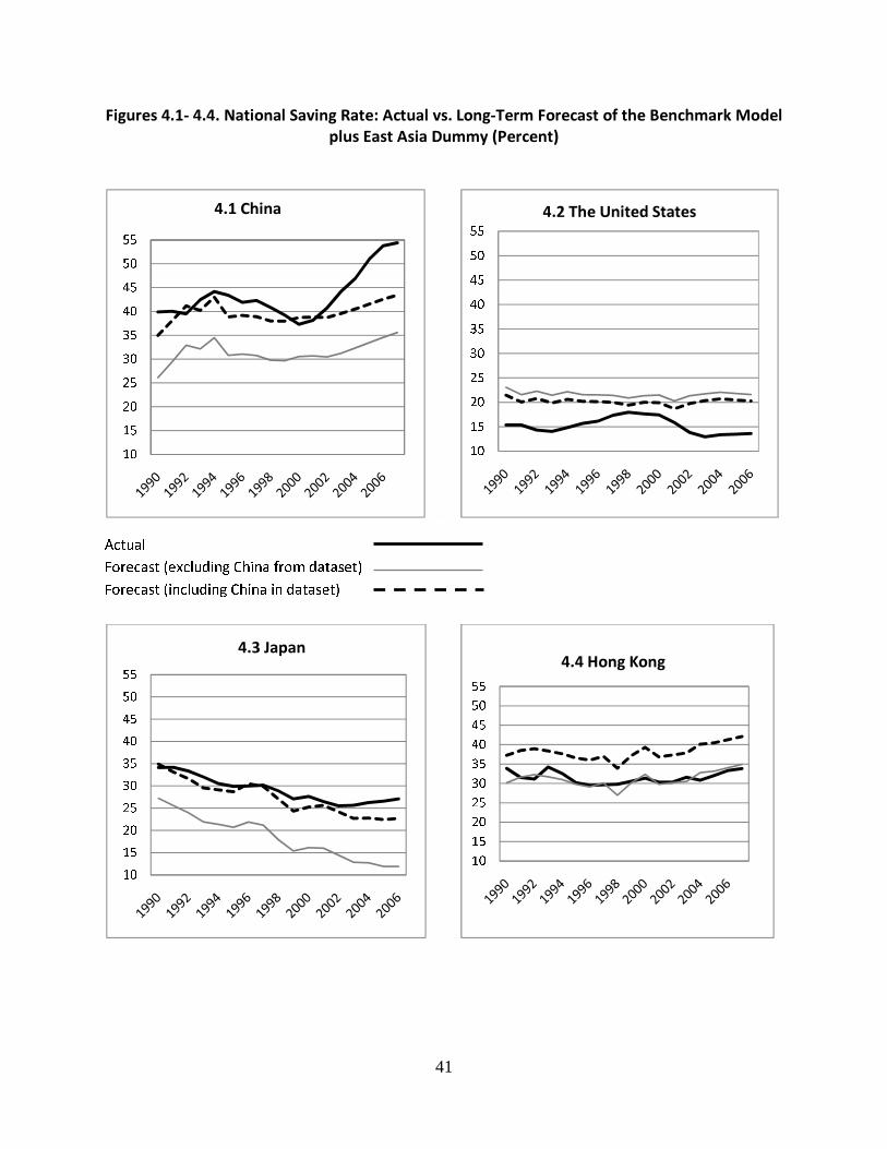
41

Figures 4.1- 4.4. National Saving Rate: Actual vs. Long-Term Forecast of the Benchmark Model

plus East Asia Dummy (Percent)

Actual

Forecast (excluding China from dataset)

Forecast (including China in dataset)

10

15

20

25

30

35

40

45

50

55

4.1 China

10

15

20

25

30

35

40

45

50

55

4.2 The United States

10

15

20

25

30

35

40

45

50

55

4.3 Japan

10

15

20

25

30

35

40

45

50

55

4.4 Hong Kong

42

Figures 4.5-4.6. National Saving Rate: Actual vs. Long-Term Forecast of the Benchmark Model

plus East Asia Dummy (Percent)

Actual

Forecast (excluding China from dataset)

Forecast (including China in dataset)

10

15

20

25

30

35

40

45

50

55

4.5 Taiwan

10

15

20

25

30

35

40

45

50

55

4.6 Korea

43

30

40

50

60

70

80

90

Figure 5. Disposable Income and Consumption in China(Percent of GNI)

Share of Disposable Income

Share of Consumption

Share of Urban Disposable IncomeSource: CEIC.

0

5

10

15

20

25

30

35

Figure 6. Household Saving Rates in China and the United States

(Percent)

China (Urban) US

Sources: CEIC and U.S. Bureau of Economic Analysis.

44

0

5

10

15

20

25

Figure 7. Composition of Gross Saving in China(Percent of GDP)

Enterprises/GDP Gov't/GDP Households/GDP

Source: CEIC.

0.0

2.0

4.0

6.0

8.0

10.0

12.0

14.0

16.0

18.0

20.0

1998 1999 2000 2001 2002 2003 2004 2005 2006 2007

Figure 8. Net Corporate Profits in China and OECD

(Percent of GNI)

China OECD Sources: CEIC and OECD.

45

0

2

4

6

8

10

12

14

1990

1991

1992

1993

1994

1995

1996

1997

1998

1999

2000

2001

2002

2003

2004

2005

2006

2007

2008

Figure 9. Government Social Spending in China and the

United States (Percent of GDP)

China US

Sources: Asian Development Bank and U.S. Bureau of Economic Analysis.

High

Income

Upper

Middle

Income

Lower

Middle

Income

Low

Income OECD USA China

Real GDP per capita (constant 2005 int'l dollar based on PPP rates)

1980-1990 13280 6158 3156 1049 20875 28420 807

1991-2000 18313 7686 3367 1037 25123 34796 1920

2001-2006 21501 9125 4070 1140 29343 40588 3613

2007 25990 11665 5019 1368 30533 43102 5084

National Saving Rate (%)

1980-1990 20.5 20.7 19.8 9.0 22.6 17.8 35.6

1991-2000 23.8 18.8 18.0 11.0 22.5 16.7 41.1

2001-2006 30.3 18.8 23.1 14.9 22.1 15.0 45.8

2007 29.5 20.0 26.7 19.8 23.0 14.3 54.4

Table 1. Real GDP per Capita and National Saving Rate

(Annual Average)

Note: Countries' income-level classifications are based on World Bank classification.

Sources: World Development Indicators and Survey of Current Business.

46

Table 2A. Dynamic Panel Regressions of National Saving Rates, Including China in Dataset

Variable Model A1 Model A2 Model A3 Model A4 Model A5 Model A6

Lagged Saving 0.51 0.499 0.535 0.5 0.564 0.532

0 0 0 0 0 0

Ln(Real GDP Per Capita) 0.036 0.038 0.032 0.035 0.03 0.027

0 0 0 0 0 0

Growth of Real GDP Per Capita 0.11 0.129 0.153 0.1 0.213 0.183

0 0 0 0 0 0

Domestic Credit/GDP -0.038 -0.024 -0.04 -0.033 -0.013 -0.025

0 0 0 0 0.037 0

Old Dependency -0.522 -0.579 -0.44 -0.477 -0.47 -0.464

0 0 0 0 0 0

Young Dependency -0.161 -0.154 -0.118 -0.107 -0.148 -0.141

0 0 0 0 0 0

Urbanization -0.04 -0.077 -0.001 -0.084 -0.049 -0.002

0.115 0.001 0.947 0 0.197 0.966

Social Spending -0.194 -0.144 -0.209 -0.047 -0.051 -0.03

0 0.02 0 0.242 0.438 0.623

Inflation 0.001

0.885

Real Interest Rate -0.146

0

Gov't Budget Balance 0.283

0

Change in Real Exchange Rate 0.038 0.031

0 0

Undervaluation 0.014 0.013

0 0

East Asia Dummy 6.761

0

Wald test 0.00 0.00 0.00 0.00 0.00 0.00

Sargan test 1.00 1.00 1.00 1.00 1.00 1.00

1st-order serial correlation 0.01 0.01 0.02 0.02 0.01 0.01

2nd-order serial correlation 0.19 0.19 0.24 0.30 0.17 0.17

3rd-order serial correlation 0.15 0.15 0.19 0.23 0.14 0.14

Number of Observations 1188 1188 1092 1110 1170 1170

Number of Countries 70 70 69 67 69 69

P-values of Wald test of joint significance and other tests for consistency of estimators:

(Estimation method: Two-step system GMM; P-values are below coefficient estimates.)

47

Table 2A'. Dynamic Panel Regressions of National Saving, Excluding China from Dataset

Variable Model A1 Model A2 Model A3 Model A4 Model A5 Model A6

Lagged Saving 0.487 0.471 0.546 0.488 0.535 0.511

0.000 0.000 0.000 0.000 0.000 0.000

Ln( Real GDP Per Capita) 0.035 0.036 0.029 0.034 0.031 0.029

0.000 0.000 0.000 0.000 0.000 0.000

Growth of Real GDP Per Capita 0.089 0.095 0.140 0.065 0.174 0.170

0.000 0.000 0.000 0.001 0.000 0.000

Domestic Credit/GDP -0.034 -0.027 -0.038 -0.034 -0.012 -0.026

0.000 0.000 0.000 0.000 0.033 0.000

Old Dependency -0.492 -0.568 -0.411 -0.428 -0.518 -0.447

0.000 0.000 0.000 0.000 0.000 0.000

Young Dependency -0.149 -0.160 -0.113 -0.104 -0.154 -0.154

0.000 0.000 0.000 0.000 0.000 0.000

Urbanization -0.024 -0.038 0.010 -0.092 -0.051 -0.016

0.483 0.053 0.663 0.002 0.271 0.740

Social Spending -0.218 -0.149 -0.177 -0.023 -0.040 -0.057

0.000 0.007 0.000 0.611 0.539 0.147

Inflation 0.002

0.839

Real Interest Rate -0.156

0.000

Gov't Budget Balance 0.289

0.000

Change in Real Exchange Rate 0.036 0.033

0.000 0.000

Undervaluation 0.012 0.010

0.000 0.000

East Asia Dummy 4.248

0.014

Wald test 0.00 0.00 0.00 0.00 0.00 0.00

Sargan test 1.00 1.00 1.00 1.00 1.00 1.00

1st-order serial correlation 0.01 0.01 0.02 0.02 0.01 0.01

2nd-order serial correlation 0.19 0.19 0.24 0.31 0.17 0.18

3rd-order serial correlation 0.15 0.15 0.19 0.23 0.14 0.14

Number of Observations 1170 1170 1074 1096 1152 1152

Number of Countries 69 69 68 66 68 68

(Estimation method: Two-step system GMM; P-values are below coefficient estimates.)

P-values of Wald test of joint significance and other tests for consistency of estimators:

48

Table 2B. Dynamic Panel Regressions of National Saving, Including China in Dataset

Variable Model B1 Model B2 Model B3 Model B4 Model B5 Model B6

Lagged Saving Rate 0.555 0.536 0.567 0.532 0.545 0.491

0 0 0 0 0 0

Ln(Real GDP Per Capita) 0.032 0.035 0.03 0.031 0.033 0.032

0 0 0 0 0 0

Growth of Real GDP Per Capita 0.089 0.069 0.103 0.065 0.144 0.138

0 0 0 0 0 0

Adjusted Growth Rate 0.01 0.012 0.005 0.008 0.008 0.007

0 0 0 0 0 0

Domestic Credit/GDP -0.033 -0.022 -0.034 -0.032 -0.002 -0.019

0 0 0 0 0.733 0

Old Dependency -0.492 -0.549 -0.459 -0.48 -0.547 -0.458

0 0 0 0 0 0

Young Dependency -0.157 -0.171 -0.1 -0.117 -0.164 -0.154

0 0 0 0 0 0

Urbanization -0.029 -0.057 -0.027 -0.047 -0.05 -0.07

0.009 0 0.079 0 0.024 0

Social Spending -0.126 -0.115 -0.111 -0.003 -0.122 -0.042

0.001 0.005 0.005 0.942 0.003 0.328

Inflation 0.013

0.162

Real Interest Rate -0.144

0

Gov't Budget Balance 0.287

0

Change in Real Exchange Rate 0.035 0.041

0 0

Undervaluation 0.011 0.013

0 0

East Asia Dummy 6.648

0

Wald test 0.00 0.00 0.00 0.00 0.00 0.00

Sargan test 1.00 1.00 1.00 1.00 1.00 1.00

1st-order serial correlation 0.01 0.01 0.02 0.02 0.01 0.01

2nd-order serial correlation 0.18 0.18 0.25 0.29 0.18 0.18

3rd-order serial correlation 0.17 0.17 0.20 0.24 0.15 0.14

Number of Observations 1188 1188 1092 1110 1170 1170

Number of Countries 70 70 69 67 69 69

(Estimation method: Two-step system GMM; P-values are below coefficient estimates.)

P-values of Wald test of joint significance and other tests for consistency of estimators:

49

Variable B1 B2 B3 B4 B5 B6

Lagged Saving 0.502 0.493 0.530 0.484 0.506 0.520

0.000 0.000 0.000 0.000 0.000 0.000

Ln(Real GDP Per Capita) 0.037 0.034 0.030 0.035 0.035 0.034

0.000 0.000 0.000 0.000 0.000 0.000

Growth of Real GDP Per Capita 0.072 0.069 0.085 0.042 0.137 0.133

0.000 0.000 0.000 0.055 0.000 0.000

Domestic Credit/GDP -0.033 -0.016 -0.038 -0.035 -0.004 -0.021

0.000 0.004 0.000 0.000 0.542 0.000

Adjusted Growth 0.006 0.007 0.003 0.003 0.006 0.007

0.000 0.002 0.160 0.053 0.000 0.000

Old Dependency -0.525 -0.519 -0.320 -0.519 -0.586 -0.532

0.000 0.000 0.000 0.000 0.000 0.000

Young Dependency -0.176 -0.152 -0.103 -0.128 -0.171 -0.165

0.000 0.000 0.000 0.000 0.000 0.000

Urbanization -0.050 -0.062 -0.043 -0.059 -0.054 -0.072

0.006 0.000 0.007 0.009 0.001 0.000

Social Spending -0.149 -0.084 -0.116 -0.021 -0.129 -0.050

0.006 0.046 0.000 0.586 0.046 0.281

Inflation 0.014

0.192

Real Interest Rate -0.130

0.000

Gov't Budget Balance 0.304

0.000

Change in Real Exchange Rate 0.030 0.032

0.000 0.000

Undervaluation 0.011 0.007

0.000 0.049

East Asia Dummy 1.756

0.598

Wald test 0.00 0.00 0.00 0.00 0.00 0.00

Sargan test 1.00 1.00 1.00 1.00 1.00 1.00

1st-order serial correlation 0.01 0.01 0.02 0.02 0.01 0.01

2nd-order serial correlation 0.19 0.19 0.26 0.31 0.18 0.18

3rd-order serial correlation 0.16 0.16 0.20 0.23 0.15 0.14

Number of Observations 1170 1170 1074 1096 1152 1152

Number of Countries 69 69 68 66 68 68

(Estimation method: Two-step system GMM; P-values are below coefficient estimates.)

Table 2B'. Dynamic Panel Regressions of National Saving, Excluding China from Dataset

P-values of Wald test of joint significance and other tests for consistency of estimators:

50

Table 2C. Dynamic Panel Regressions of National Saving, Including China in Dataset

Variable Model C1 Model C2 Model C3 Model C4 Model C5 Model C6

Lagged Saving Rate 0.535 0.524 0.567 0.5 0.545 0.507

0 0 0 0 0 0

Ln(Real GDP Per Capita) 0.034 0.035 0.03 0.033 0.032 0.03

0 0 0 0 0 0

Growth of Real GDP Per Capita 0.075 0.084 0.105 0.068 0.142 0.127

0.01 0.003 0 0.01 0 0

Adjusted Growth Rate 0.009 0.01 0.005 0.005 0.011 0.008

0 0 0.001 0.046 0.006 0.005

Domestic Credit/GDP -0.036 -0.021 -0.034 -0.036 -0.011 -0.009

0 0 0 0 0.073 0.233

Old Dependency -0.488 -0.549 -0.441 -0.485 -0.592 -0.607

0 0 0 0 0 0

Young Dependency -0.173 -0.165 -0.098 -0.129 -0.169 -0.147

0 0 0 0 0 0

Urbanization -0.036 -0.065 -0.027 -0.049 -0.035 -0.033

0.038 0 0.094 0.001 0.086 0.089

Social Spending -0.148 -0.093 -0.115 -0.023 -0.07 0.01

0.003 0.055 0.005 0.562 0.241 0.812

Asian Crisis Dummy 0.348 0.507 0.155 0.243 0.053 0.231

0.002 0 0.074 0 0.632 0.014

Inflation 0.019

0.031

Real Interest Rate -0.143

0

Gov't Budget Balance 0.274

0

Change in Real Exchange Rate 0.039 0.027

0 0

Undervaluation 0.013 0.013

0 0

East Asia Dummy 7.023

0.054

Number of Observations 1188 1188 1092 1110 1170 1170

Number of Countries 70 70 69 67 69 69

(Estimation method: Two-step system GMM; P-values are below coefficient estimates.)

51

Table 2C'. Dynamic Panel Regressions of National Saving, Excluding China from Dataset

Variable Model C1 Model C2 Model C3 Model C4 Model C5 Model C6

Lagged Saving Rate 0.513 0.467 0.53 0.515 0.546 0.497

0 0 0 0 0 0

Ln(Real GDP Per Capita) 0.035 0.038 0.03 0.032 0.029 0.031

0 0 0 0 0 0

Growth of Real GDP Per Capita 0.077 0.094 0.09 0.055 0.137 0.085

0 0 0.001 0.003 0 0.04

Adjusted Growth Rate 0.004 0.002 0.001 0.004 0.009 0.01

0.014 0.504 0.76 0.044 0.004 0.005

Domestic Credit/GDP -0.035 -0.022 -0.038 -0.035 -0.011 -0.01

0 0 0 0 0.059 0.125

Old Dependency -0.508 -0.531 -0.329 -0.494 -0.474 -0.577

0 0 0 0 0 0

Young Dependency -0.161 -0.164 -0.1 -0.115 -0.147 -0.16

0 0 0 0 0 0

Urbanization -0.043 -0.091 -0.042 -0.046 -0.027 -0.039

0.007 0.001 0.013 0 0.144 0.01

Social Spending -0.13 -0.09 -0.117 0 -0.076 0

0 0.195 0.001 0.991 0.141 0.997

Asian Crisis Dummy 0.369 0.559 0.137 0.147 0.081 0.159

0.001 0 0.254 0.046 0.433 0.172

Inflation 0.012

0.117

Real Interest Rate -0.132

0

Gov't Budget Balance 0.286

0

Change in Real Exchange Rate 0.036 0.029

0 0

Undervaluation 0.012 0.014

0 0.001

East Asia Dummy 6.383

0.196

Number of Observations 1170 1170 1074 1096 1152 1152

Number of Countries 69 69 68 66 68 68

(Estimation method: Two-step system GMM; P-values are below coefficient estimates.)

52

Table 3. Comparisons of Short-term and Long-term coefficient Estimates

Dependent variable: Saving rate This Paper IMF LHS This Paper IMF LHS

Lagged saving rate 0.510 0.62 0.38

Growth rate of per capita GDP (GNDI in LHS) 0.110 0.17 0.45 0.224 0.45 0.73

Real per capita GDP (GNDI in LHS) 0.036 0.102 0.073 0.16

Domestic credit/GDP (GNDI in LHS) -0.038 -3.47 -0.36 -0.078 -9.13 -0.58

Old dependency -0.522 -0.44 -0.77 -1.065 -1.16 -1.24

Young dependency -0.161 -0.16 -0.329 -0.26

Urbanization -0.040 -0.5 -0.082 -0.81

Real interest rate -0.146 -0.136 -0.298 -0.22

Government saving 0.283 0.27 0.578 0.71

Real exchange rate change 0.038 0.08 0.057 0.078 0.21 0.09

Inflation 0.001 0.18 0.002 0.29

Note: The comparison needs to be taken in perspective mainly for the following reasons:

1. LHS refers to Loayza et al. (2000). Both LHS and IMF (2005) include terms of trade growth, not real exchange rate change.

2. LHS data were from 1965 to 1994, the IMF data were from1972 to 2004 , and this paper's data were from 1980 to 2007.

3. This paper's coefficient estimates are taken from Table 2A. Estimates of inflation, real interest rate, and government saving

are taken from models A2, A3, and A4 respectively. Other coefficients are from Model A5.

4. The dependent variable is somewhat different in the three papers: it is private saving/gross national disposable income (GNDI) in LHS;

national saving/gross national income(GNI) in this paper, and national saving/GDP in IMF.

Implied Long-Term Estimates

Table 4. Unexplained Saving Rates by Model (percent; average of sample period)

(unexplained saving = national saving - long-term forecast)

(% forecast error = long-term forecast/national saving -1)

China

Regression

Unexplained

Saving

% Forecast

Error

Unexplained

Saving

% Forecast

Error

Unexplained

Saving

% Forecast

Error

B1 16.1 0% -0.1 0% -1.1 0%

B2 13.7 0% -0.3 0% -1.1 0%

B3 15.8 0% -0.3 0% -1.4 0%

B4 19.8 0% -0.3 0% -1.3 0%

B5 10.3 0% -0.1 0% -0.8 0%

B6 3.7 0% 1.1 0% 0.5 0%

B1 17.6 0% 0.1 0% -0.5 0%

B2 16.5 0% -0.3 0% -0.6 0%

B3 19.1 0% -0.3 0% -0.3 0%

B4 21.3 0% 0.3 0% -0.6 0%

B5 12.2 0% 0.4 0% -0.3 0%

B6 11.9 0% 0.5 0% -0.1 0%

Models Estimated with the Full Dataset (Table 2B)

Models Estimated Excluding China from Dataset (Table 2B')

OECD All Countries

53

Table 4.1 Actual and Model Forecasts of National Saving Rates (percent)

(unexplained saving = national saving - long-term forecast)

(% deviation = national saving rate/long-term forecast -1)

Country

Saving

Rate

Unexplained

Saving

%

deviation Country

Saving

Rate

Unexplained

Saving

%

deviation

Bhutan 49.07 21.16 76% Guatemala 12.86 -1.16 -8%

Honduras 24.31 10.63 78% Ireland 23.31 -1.30 -5%

China 43.34 10.31 31% Portugal 21.97 -1.48 -6%

Mongolia 29.86 10.13 51% Hong Kong, China 31.48 -1.55 -5%

Sweden 20.74 9.98 93% Peru 21.87 -1.56 -7%

Norway 28.04 8.40 43% Tonga 15.32 -1.61 -9%

Singapore 46.57 6.49 16% Chile 23.84 -1.92 -7%

Belgium 22.23 6.07 38% Hungary 19.68 -2.21 -10%

Papua New Guinea 26.47 6.04 30% Paraguay 15.92 -2.46 -13%

Luxembourg 34.15 5.95 21% Thailand 32.47 -2.49 -7%

Nepal 22.25 5.14 30% Nicaragua 12.37 -2.55 -17%

India 30.50 5.00 20% Georgia 18.27 -2.73 -13%

Switzerland 30.18 4.98 20% New Zealand 18.88 -2.93 -13%

Philippines 24.78 4.98 25% South Korea 34.30 -3.04 -8%

Japan 30.08 4.78 19% Fiji 21.62 -3.75 -15%

Brunei 49.87 4.44 10% Australia 21.40 -3.92 -15%

Venezuela 28.69 4.07 17% Poland 18.61 -4.15 -18%

Jamaica 23.72 3.96 20% Mexico 20.74 -4.79 -19%

Bangladesh 23.61 3.52 18% Greece 17.22 -4.89 -22%

Denmark 21.06 3.05 17% Slovak Republic 23.30 -4.94 -17%

Uruguay 13.56 2.37 21% Iceland 16.62 -6.63 -29%

Panama 24.88 1.89 8% El Salvador 13.92 -6.67 -32%

France 19.42 1.73 10% Vanuatu 11.91 -7.40 -38%

Finland 23.90 1.70 8% Canada 20.17 -7.61 -27%

Argentina 17.81 1.41 9% Brazil 15.34 -7.68 -33%

Germany 20.42 1.31 7% Colombia 16.86 -7.87 -32%

Spain 21.94 0.98 5% Sri Lanka 21.15 -9.07 -30%

Austria 22.46 0.84 4% Taiwan 26.98 -9.90 -27%

Bolivia 14.92 0.74 5% Turkey 16.08 -10.12 -39%

Netherlands 25.28 0.43 2% Cambodia 12.84 -10.40 -45%

Italy 21.25 0.38 2% Kyrgyz Republic 10.61 -10.43 -50%

Czech Republic 25.19 0.28 1% Costa Rica 15.01 -10.46 -41%

Indonesia 27.17 -0.61 -2% Tajikistan 11.77 -11.10 -49%

United Kingdom 16.15 -0.77 -5% United States 15.95 -11.13 -41%

Dominican Republic 21.63 -0.87 -4% Trinidad and Tobago 26.56 -11.38 -30%

OECD 22.31 -0.10 0%

All 70 Countries in Sample 22.25 -0.77 -3%

Note: Each country's saving rate is the average over the years for which data are available for that country.

The sample period is from 1980 to 2007, but some countries do not have data for the entire sample period.

Model = Model B5 of Table 2B , estimated with China in dataset

54

Table 4.2 Actual and Model Forecasts of National Saving Rates (percent)

(unexplained saving = national saving - long-term forecast)

(% deviation = national saving rate/long-term forecast -1)

Country

Saving

Rate

Unexplained

Saving

%

Deviation Country

Saving

Rate

Unexplained

Saving

%

Deviation

Bhutan 49.07 22.01 81% Hong Kong, China 31.48 -0.69 -2%

China 43.34 12.22 39% Ireland 23.31 -0.85 -4%

Honduras 24.31 10.65 78% Portugal 21.97 -0.96 -4%

Mongolia 29.86 10.64 55% Peru 21.87 -1.22 -5%

Sweden 20.74 10.27 98% Guatemala 12.86 -1.26 -9%

Norway 28.04 8.75 45% Chile 23.84 -1.31 -5%

Singapore 46.57 7.33 19% Georgia 18.27 -1.42 -7%

Luxembourg 34.15 6.68 24% Tonga 15.32 -1.46 -9%

Belgium 22.23 6.47 41% Thailand 32.47 -1.47 -4%

Papua New Guinea 26.47 6.27 31% Hungary 19.68 -1.71 -8%

India 30.50 6.10 25% South Korea 34.30 -2.19 -6%

Nepal 22.25 5.73 35% Nicaragua 12.37 -2.25 -15%

Japan 30.08 5.70 23% Paraguay 15.92 -2.41 -13%

Switzerland 30.18 5.59 23% New Zealand 18.88 -2.59 -12%

Philippines 24.78 5.31 27% Fiji 21.62 -3.44 -14%

Brunei 49.87 5.00 11% Australia 21.40 -3.48 -14%

Bangladesh 23.61 4.48 23% Poland 18.61 -3.71 -17%

Venezuela 28.69 4.26 17% Slovak Republic 23.30 -4.36 -16%

Jamaica 23.72 4.24 22% Greece 17.22 -4.44 -20%

Denmark 21.06 3.36 19% Mexico 20.74 -4.61 -18%

Uruguay 13.56 2.62 24% Iceland 16.62 -6.27 -27%

Panama 24.88 2.24 10% El Salvador 13.92 -6.51 -32%

France 19.42 2.09 12% Canada 20.17 -7.03 -26%

Finland 23.90 2.04 9% Brazil 15.34 -7.31 -32%

Germany 20.42 1.79 10% Vanuatu 11.91 -7.33 -38%

Argentina 17.81 1.73 11% Colombia 16.86 -7.56 -31%

Spain 21.94 1.50 7% Sri Lanka 21.15 -8.23 -28%

Austria 22.46 1.32 6% Cambodia 12.84 -8.82 -41%

Netherlands 25.28 0.99 4% Taiwan 26.98 -9.16 -25%

Bolivia 14.92 0.87 6% Tajikistan 11.77 -9.35 -44%

Italy 21.25 0.82 4% Kyrgyz Republic 10.61 -9.56 -47%

Czech Republic 25.19 0.78 3% Turkey 16.08 -9.87 -38%

Indonesia 27.17 0.20 1% Costa Rica 15.01 -10.14 -40%

United Kingdom 16.15 -0.34 -2% United States 15.95 -10.44 -40%

Dominican Republic 21.63 -0.46 -2% Trinidad and Tobago 26.56 -10.80 -29%

OECD 22.31 0.39 2%

All 70 Countries in Sample 22.25 -0.26 -1%

Note: Each country's saving rate is the average over the years for which data are available for that country.

The sample period is from 1980 to 2007, but some countries do not have data for the entire sample period.

Model = Model B5 of Table 2B', estimated without China in dataset

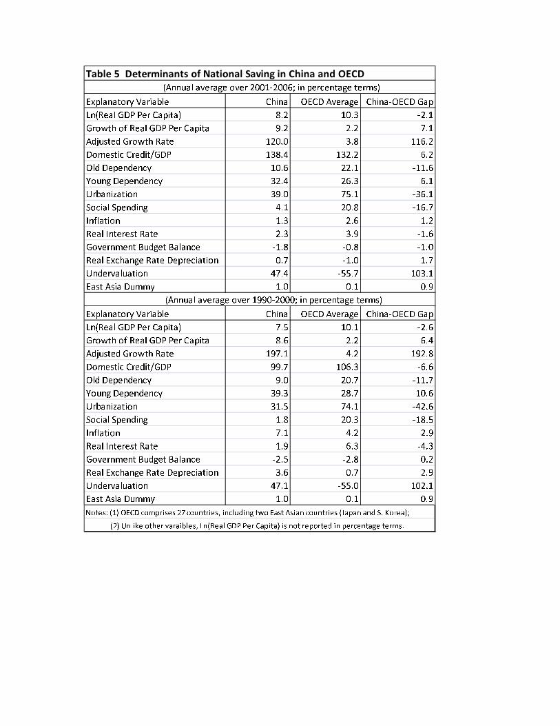
Explanatory Variable China OECD Average China-OECD Gap

Ln(Real GDP Per Capita) 8.2 10.3 -2.1

Growth of Real GDP Per Capita 9.2 2.2 7.1

Adjusted Growth Rate 120.0 3.8 116.2

Domestic Credit/GDP 138.4 132.2 6.2

Old Dependency 10.6 22.1 -11.6

Young Dependency 32.4 26.3 6.1

Urbanization 39.0 75.1 -36.1

Social Spending 4.1 20.8 -16.7

Inflation 1.3 2.6 -1.2

Real Interest Rate 2.3 3.9 -1.6

Government Budget Balance -1.8 -0.8 -1.0

Real Exchange Rate Depreciation 0.7 -1.0 1.7

Undervaluation 47.4 -55.7 103.1

East Asia Dummy 1.0 0.1 0.9

Explanatory Variable China OECD Average China-OECD Gap

Ln(Real GDP Per Capita) 7.5 10.1 -2.6

Growth of Real GDP Per Capita 8.6 2.2 6.4

Adjusted Growth Rate 197.1 4.2 192.8

Domestic Credit/GDP 99.7 106.3 -6.6

Old Dependency 9.0 20.7 -11.7

Young Dependency 39.3 28.7 10.6

Urbanization 31.5 74.1 -42.6

Social Spending 1.8 20.3 -18.5

Inflation 7.1 4.2 2.9

Real Interest Rate 1.9 6.3 -4.3

Government Budget Balance -2.5 -2.8 0.2

Real Exchange Rate Depreciation 3.6 0.7 2.9

Undervaluation 47.1 -55.0 102.1

East Asia Dummy 1.0 0.1 0.9

(2) Unlike other varaibles, Ln(Real GDP Per Capita) is not reported in percentage terms.

Table 5 Determinants of National Saving in China and OECD

(Annual average over 2001-2006; in percentage terms)

(Annual average over 1990-2000; in percentage terms)

Notes: (1) OECD comprises 27 countries, including two East Asian countries (Japan and S. Korea);

56

Table 6.1 Contributions of Explanatory Variables to the China-OECD Saving Gaps (percent)

Explanatory Variable Model B1 Model B2 Model B3 Model B4 Model B5 Model B6

Ln(Real GDP per Capita) -14.9 -15.6 -14.4 -13.7 -15.0 -13.0

Growth of Real GDP per Capita 1.4 1.1 1.7 1.0 2.2 1.9

Adjusted Growth 2.6 3.0 1.3 2.0 2.0 1.6

Domestic Credit/GDP -0.5 -0.3 -0.5 -0.4 0.0 -0.2

Old Dependency 12.8 13.7 12.2 11.8 13.9 10.4

Young Dependency -2.2 -2.3 -1.4 -1.5 -2.2 -1.9

Urbanization 2.4 4.4 2.3 3.6 4.0 5.0

Social Spending 4.7 4.1 4.3 0.1 4.5 1.4

Inflation 0.0

Real Interest Rate 0.5

Gov't Budget Balance -0.6

Change in Real Exchange Rate 0.4 0.4

Undervaluation 2.5 2.6

East Asia Dummy 12.0

Total contribution to saving gap 6.3 8.1 6.1 2.3 12.3 20.2

China-OECD saving rate gap 23.6 23.6 23.6 23.6 23.6 23.6

Explanatory Variable Model B1 Model B2 Model B3 Model B4 Model B5 Model B6

Ln(Real GDP per Capita) -18.7 -19.6 -18.0 -17.2 -18.8 -16.3

Growth of Real GDP per Capita 1.3 1.0 1.5 0.9 2.0 1.7

Adjusted Growth 4.3 5.0 2.2 3.3 3.4 2.7

Domestic Credit/GDP 0.5 0.3 0.5 0.4 0.0 0.2

Old Dependency 13.0 13.9 12.5 12.0 14.1 10.6

Young Dependency -3.7 -3.9 -2.4 -2.6 -3.8 -3.2

Urbanization 2.8 5.2 2.7 4.3 4.7 5.9

Social Spending 5.2 4.6 4.7 0.1 5.0 1.5

Inflation 0.1

Real Interest Rate 1.4

Gov't Budget Balance 0.2

Change in Real Exchange Rate 0.1 0.1

Undervaluation 2.5 2.6

East Asia Dummy 12.1

Total contribution to saving gap 4.7 6.6 5.1 1.4 9.2 17.9

China-OECD saving rate gap 18.4 18.4 18.4 18.4 18.4 18.4

Note: Marginal contribution of X = (X in China - X in OECD)/(1-coefficient of lag saving); the coefficients

used are taken from regressions presented in Table 2B, which includes China in the dataset.

Based on coefficients estimated with China in dataset; 2001-2006

Based on coefficients estimated with China in dataset; 1990-2000

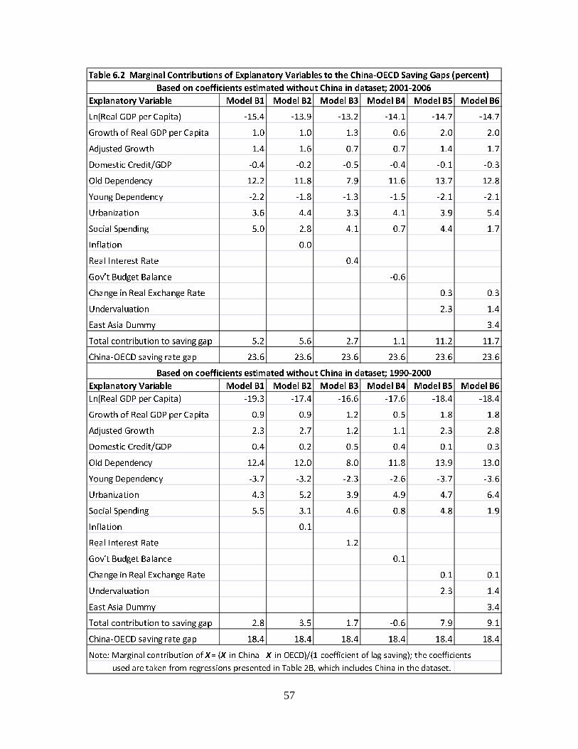
57

Table 6.2 Marginal Contributions of Explanatory Variables to the China-OECD Saving Gaps (percent)

Explanatory Variable Model B1 Model B2 Model B3 Model B4 Model B5 Model B6

Ln(Real GDP per Capita) -15.4 -13.9 -13.2 -14.1 -14.7 -14.7

Growth of Real GDP per Capita 1.0 1.0 1.3 0.6 2.0 2.0

Adjusted Growth 1.4 1.6 0.7 0.7 1.4 1.7

Domestic Credit/GDP -0.4 -0.2 -0.5 -0.4 -0.1 -0.3

Old Dependency 12.2 11.8 7.9 11.6 13.7 12.8

Young Dependency -2.2 -1.8 -1.3 -1.5 -2.1 -2.1

Urbanization 3.6 4.4 3.3 4.1 3.9 5.4

Social Spending 5.0 2.8 4.1 0.7 4.4 1.7

Inflation 0.0

Real Interest Rate 0.4

Gov't Budget Balance -0.6

Change in Real Exchange Rate 0.3 0.3

Undervaluation 2.3 1.4

East Asia Dummy 3.4

Total contribution to saving gap 5.2 5.6 2.7 1.1 11.2 11.7

China-OECD saving rate gap 23.6 23.6 23.6 23.6 23.6 23.6

Explanatory Variable Model B1 Model B2 Model B3 Model B4 Model B5 Model B6

Ln(Real GDP per Capita) -19.3 -17.4 -16.6 -17.6 -18.4 -18.4

Growth of Real GDP per Capita 0.9 0.9 1.2 0.5 1.8 1.8

Adjusted Growth 2.3 2.7 1.2 1.1 2.3 2.8

Domestic Credit/GDP 0.4 0.2 0.5 0.4 0.1 0.3

Old Dependency 12.4 12.0 8.0 11.8 13.9 13.0

Young Dependency -3.7 -3.2 -2.3 -2.6 -3.7 -3.6

Urbanization 4.3 5.2 3.9 4.9 4.7 6.4

Social Spending 5.5 3.1 4.6 0.8 4.8 1.9

Inflation 0.1

Real Interest Rate 1.2

Gov't Budget Balance 0.1

Change in Real Exchange Rate 0.1 0.1

Undervaluation 2.3 1.4

East Asia Dummy 3.4

Total contribution to saving gap 2.8 3.5 1.7 -0.6 7.9 9.1

China-OECD saving rate gap 18.4 18.4 18.4 18.4 18.4 18.4

Note: Marginal contribution of X = (X in China - X in OECD)/(1-coefficient of lag saving); the coefficients

used are taken from regressions presented in Table 2B, which includes China in the dataset.

Based on coefficients estimated without China in dataset; 2001-2006

Based on coefficients estimated without China in dataset; 1990-2000

58

REFERENCES

Anderson, T. W. and C. Hsiao (1982), “Formulation and Estimation of Dynamic Models using Panel Data,” Journal of Econometrics, vol. 18, no.1, pp. 47–82. Arellano, M. and S. Bond (1991), “Some Tests of Specification for Panel Data: Monte Carlo Evidence and an Application to Employment Equations,” Review of Economic Studies, vol. 58, no. 2, pp. 277–297.

Arellano, M. and O. Bover (1995), “Another Look at the Instrumental Variable Estimation of Error-Component Models, Journal of Econometrics, vol. 68, no. 1, pp. 29–51.

Aziz, Jahangir and Li Cui (2007), “Explaining China’s Low Consumption: The Neglected Role of Household Income,” International Monetary Fund, IMF Working Paper No. 07/181.

Bai, C., C. Hsieh, and Y. Qian (2006), “Return to Capital in China,” National Bureau of Economic Research, NBER Working Paper No. 12755.

Baek, Seung-Wook (2005), “Does China Follow the East Asian Development Model?” Journal of Contemporary Asia, vol. 35, no. 4, pp. 485–498.

Blanchard, Olivier and Francesco Giavazzi (2006), “Rebalancing Growth in China: A Three-Handed Approach,” China and World Economy, vol. 14, no. 4, pp. 1–20.

Blundell, R. and S. Bond (1997), “Initial Conditions and Moment Restrictions in Dynamic Panel Data Models,” University College London, Discussion Paper No. 97-07.

Boltho, Andrea and Maria Weber (2009), “Did China Follow the East Asian Development Model?” The European Journal of Comparative Economics, vol. 6, no. 2, pp. 267–286.

Bosworth, Barry (1993), “Saving and Investment in a Global Economy,” The Brookings Institution, Washington, DC.

Caballero, Ricardo (2009), “The ‘Other’ Imbalance and the Financial Crisis,” National Bureau of Economic Research, NBER Working Paper No. 15636.

Carroll, C.D. and D.N. Weil (1994), “Saving and Growth: A Reinterpretation,” Carnegie – Rochester Conference Series on Public Policy 40, pp. 133–192.

Carroll, Christopher D., Jody Overland, and David N. Weil (2000), “Saving and Growth with Habit Formation,” American Economic Review, vol. 90, no. 3, pp. 341–355.

Chamberlain, G. (1984), “Panel Data,” Handbook of Econometrics, Z. Griliches and M. D. Intriligator (eds.), Amsterdam: Elsevier, vol. 2, pp. 1247–1313.

Chamon, Marcos and Eswar Prasad (2010), “Why Are Saving Rates of Urban Households in China Rising?” American Economic Journal: Macroeconomics, vol. 2, no. 1, pp. 93–130.

59

Cheung, Ying-Wong, Menzie D. Chinn, and Eiji Fujii (2007), “The Overvaluation of Renminbi Undervaluation,” Journal of International Money and Finance, vol. 26, no. 5, pp. 762–785.

Chinn, Menzie D. and Eswar S. Prasad (2003), “Medium-Term Determinants of Current Accounts in Industrial and Developing Countries: An Empirical Exploration,” Journal of International Economics, vol. 59, no. 1, pp. 47–76.

Choi, Horag, Mark Nelson, and Donggyu Sul (2008), “Endogenous Discounting, the World Saving Glut and the U.S. Current Account,” Journal of International Economics, vol. 75, no. 1, pp. 30–53.

Congressional Budget Office (2004), “The Decline in the U.S. Current-Account Balance Since 1991,” Economic and Budget Issue Brief. Congressional Budget Office (2005), “Recent Shifts in Financing the U.S. Current Account Deficit,” Economic and Budget Issue Brief. Congressional Budget Office (2007), “Will the U.S. Current Account Have a Hard or Soft Landing?” Economic and Budget Issue Brief. Dooley, Michael, David Folkerts-Landau, and Peter Garber (2003), “An Essay on the Revived Bretton Woods System,” National Bureau of Economic Research, NBER Working Paper No. 9971. Dooley, Michael, David Folkerts-Landau, and Peter M. Garber (2004), “The U.S. Current Account Deficit and Economic Development: Collateral for a Total Return Swap,” National Bureau of Economic Research, NBER Working Paper No. 10727. Edwards, Sebastian (1996), “Why Are Latin America's Savings Rates So Low? An International Comparative Analysis,” Journal of Development Economics, vol. 51, no. 1, pp. 5–44.

Easterly, W., N. Loayza, and P. Montiel (1997), “Has Latin America's Post-Reform Growth Been Disappointing?” Journal of International Economics, vol. 43, no. 3/4, pp. 287–312.

Eichengreen , Barry (2004), “Global Imbalances and the Lessons of Bretton Woods,” National Bureau of Economic Research, NBER Working Paper No.10497.

Gavin M., R. Hausmann, and E. Talvi (1997), “Saving Behavior in Latin America: Overview and Policy Issues,” Promoting Savings in Latin America, Ricardo Hausmann and Helmont Reisen, eds., Organization of Economic Cooperation and Development and Inter-America Development Bank: Paris, pp. 13–43.

Goldstein, Morris (2007), “A (Lack of) Progress Report on China’s Exchange Rate Policies,” Peterson Institute for International Economics, Working Paper No. 07-5.

60

Haggard, Stephan (1988), “The Politics of Industrialization in the Republic of Korea and Taiwan,” Achieving Industrialization in East Asia, Helen Hughes, ed., Cambridge University Press: New York, ch. 9. Harberger, Arnold C. (1950), “Currency Depreciation, Income, and the Balance of Trade,” Journal of Political Economy vol. 58, no. 1, pp. 47–60. Holtz-Eakin, D., W. Newey, and H. Rosen (1988), “Estimating Vector Autoregressions with Panel Data,” Econometrica, vol. 56, no. 6, pp. 1371–1395.

Hirono, Ryokichi (1988), “Japan: Model for East Asian Industrialization?” Achieving Industrialization in East Asia, Helen Hughes, ed., Cambridge University Press: New York, ch. 8.

Hung, Juann H. and Young J. Kim (2006), “Implications of Past Currency Crises for the U.S. Current Account Adjustment,” Congressional Budget Office, Working Paper No. 2006-07.

International Monetary Fund (2005), “Global Imbalances: A Saving and Investment Perspective,” World Economic Outlook, pp. 91–124.

Kraay, Aart (2000), “Household Saving in China,” World Bank Economic Review, vol. 14, no. 3, pp. 545–570.

Korinek, A. and Luis Serven (2010), “Undervaluation Through Foreign Reserve Accumulation: Static Losses, Dynamic Gains,” World Bank Policy Research Working Paper No. 5250.

Kuijs, Louis (2005), “Investment and Saving in China,” World Bank Policy Research Working Paper No. 3633.

Kuijs, Louis (2006), “How Will China’s Saving–Investment Balance Evolve?” World Bank Policy Research Working Paper No. 3958.

Kuijs, Louis and T. Wang (2006), “ China’s Patten of Growth: Moving to Sustainability and Reducing Inequality,” China & World Economy, no.1. Laursen, Svend and Lloyd A. Metzler (1950), “Flexible Exchange Rates and the Theory of Employment,” Review of Economics and Statistics vol. 32, no.4, pp. 281-99. Levy-Yeyati E. and F. Sturzenegger (2007), “Fear of Appreciation,” World Bank Policy Research Working Paper No. 4387.

Loayza, Norman, Klaus Schmidt-Hebbel, and Luis Serven (2000), “What Drives Private Saving Across the World?” The Review of Economics and Statistics, vol. 82, no. 2, pp. 165–181.

Ma, Guonan and Wang Yi (2010), “China’s High Saving Rate: Myth and Reality,” Bank for International Settlements, Working Paper No. 312.

Masson, Paul R., Tamim Bayoumi, and Hossein Samiei (1998), “International Evidence on the Determinants of Private Saving,” World Bank Economic Review, vol. 12, no. 3, pp. 483–501.

61

McKinnon, Ronald (2007), “Why China Should Keep Its Dollar Peg: A Historical Perspective from Japan,” Stanford University Working Paper No. 323. Modigliani, Franco (1970), “The Life Cycle Hypothesis of Saving and Intercountry Differences in the Saving Ratio,” Induction, Growth and Trade: Essays in Honor of Sir Roy Harrod, W.A. Eltis, M.F. Scott, and J.N. Wolfe, eds., Oxford, pp. 197–225.

Modigliani, Franco and Shi Larry Cao (2004), “The Chinese Saving Puzzle and the Life Cycle Analysis,” Journal of Economic Literature, vol. 42, no.1, pp.145–70.

Obstfeld, Maurice and Kenneth Rogoff (2005), “The Unsustainable U.S. Current Account Revisited,” National Bureau of Economic Research, Working Paper No. 10864. O’Malley, William J. (1988), “Culture and Industrialization,” Achieving Industrialization in East Asia, Helen Hughes, ed., Cambridge University Press: New York, ch. 11.

Park, Donghyun, and Kwanho Shin (2009), “Saving, Investment and Current Account Surplus in Developing Asia,” manuscript, available at https://editorialexpress.com/cgi-bin/conference/download.cgi?db name=FEMES09&paper id=399.

Pettis, Michael (2010), “Bad Loans Could Take Their Toll on China’s Growth,” Financial Times, April 21.

Phelps, Edmund S. (1961), “The Golden Rule of Accumulation: A Fable for Growth men,” American Economic Review, vol. 51, no. 4, pp. 638–43.

Phelps, Edmund S. (1965), “Second Essay on the Golden Rule of Accumulation,” American Economic Review, vol. 55, no. 4, pp. 793–814. Rodrik, Dani (2000), “Saving Transitions,” World Bank Economic Review, vol. 14, no. 3, pp. 481–507. Rodrik, Dani (2008), “The Real Exchange Rate and Economic Growth,” Brookings Papers on Economic Activity, 2, pp. 365-412. Rodrik, Dani (2009), “Making Room for China in the World Economy,” available at http://www.hks.harvard.edu/fs/drodrik/Research papers/Making room for China.pdf.

Roubini, Nouriel and Brad Setser (2005), “The Sustainability of the U.S. External Imbalances,” Ifo Institute for Economic Research, CESifo Forum, 1, pp. 8–15. Sinha, Dipendra and Tapen Sinha (2008), “Relationships Among Household Saving, Public Saving, Corporate Saving and Economic Growth in India,” Journal of International Development, vol. 20, no. 2, pp. 181–186.

Spence, Michael (2010), “The West is Wrong to Obsess About the Renminbi,” Financial Times, January 21.

62

Terrones, Marco, Roberto Cardarelli, Enrique Mendoza, and Chris Otrok (2005), “Global Imbalances: A Saving and Investment Perspective,” International Monetary Fund, World Economic Outlook, pp. 91–124.

Wei, Shang-Jin and Xiaobo Zhang (2009), “The Competitive Saving Motive: Evidence from Rising Sex Ratios and Saving Rates in China,” National Bureau of Economic Research, Working Paper No. 15093.

Wolf, Martin (2010), “Evaluating the Renminbi Manipulation,” Financial Times, April 6.

World Bank (1993), “The East Asian Miracle: Economic Growth and Public Policy,” Oxford University Press: New York.

Xu, Min (2005), “Resolution of Non-Performing Loans in China,” manuscript, The Leonard N. Stern School of Business, New York University.

Zhou, Xiaochuan (2009), “On Savings Ratio,” The People’s Bank of China, governor’s speech.