why does inflation differ across countries? · 9 why does inflation differ across countries? marta...

This PDF is a selection from an out-of-print volume from the National Bureauof Economic Research

Volume Title: Reducing Inflation: Motivation and Strategy

Volume Author/Editor: Christina D. Romer and David H. Romer, Editors

Volume Publisher: University of Chicago Press

Volume ISBN: 0-226-72484-0

Volume URL: http://www.nber.org/books/rome97-1

Conference Date: January 11-13, 1996

Publication Date: January 1997

Chapter Title: Why Does Inflation Differ across Countries?

Chapter Author: Marta Campillo, Jeffrey A. Miron

Chapter URL: http://www.nber.org/chapters/c8889

Chapter pages in book: (p. 335 - 362)

9 Why Does Inflation Differ across Countries? Marta Campillo and Jeffrey A. Miron

9.1 Introduction

The inflation performance of economies is interesting to academic economists, policymakers, politicians, and the electorate. Economists are in broad agreement about how policy actions affect inflation rates, and they share much common ground about the factors that policy should consider in choosing an economy’s inflation rate.

Perhaps surprisingly, given the relative consensus about what determines inflation and about how inflation rates should be set, inflation differs substantially across countries. Figure 9.1 graphs the inflation rate by country for the 1973-94 period. The highest average inflation rate in the sample is 127% (Bra- zil) and the lowest is 2% (Central African Republic). Even excluding what might be considered special cases, inflation rates differ markedly. If these differences reflect differences in the factors that determine desired inflation, given the constraints each economy faces, then the differences provide support both for economic models of inflation and for the notion that policymakers choose inflation in a reasonably intelligent fashion. If the differences in inflation cannot be at least approximately attributed to factors that should explain these differences, then either economists’ models or policymakers’ actions, or both, are lacking.

This paper attempts to explain the differences in inflation performance across countries. Some earlier research has examined this topic, but it has considered only a few of the factors that might be empirically important determi-

Marta Campillo is a graduate student in economics at Boston University. Jeffrey A. Miron is professor of economics at Boston University and a research associate of the National Bureau of Economic Research.

Comments from Maury Ohstfeld, Christina Romer, David Romer, Greg Mankiw, and seminar participants at Harvard, Brown, Yale, Colgate, and Hamilton are appreciated. Adam Posen kindly provided his data on financial opposition to inflation.

335

336 Marta Campillo and Jeffrey A. Miron

120

100

80

60

40

20

0

Countries in alphabetic order

Fig. 9.1 Average annual inflation rates, 1973-94, 110 countries

nants of inflation rates. In particular, existing research has focused on institutional characteristics like central bank independence (Grilli, Masciandaro, and Tabellini 1991; Cukierman, Webb, and Neyapti 1992), on the degree of openness (Romer 1993; Lane 1995), and on financial-sector opposition to inflation (Posen 1993, 1995). These factors are potentially important determinants of inflation, and existing evidence supports a role for each. Nevertheless, a priori reasoning suggests a number of additional factors that should matter as well.

We analyze the degree to which prior inflation experience, optimal tax considerations, and time-consistency issues other than central bank independence. as well as the factors considered in the existing literature, are important determinants of inflation rates across countries. The basic approach, as in earlier papers, is cross-country regressions of average inflation rates on country characteristics. The innovation of this paper is simply to include a broader range of country characteristics on the right-hand side.

The paper provides several interesting conclusions relative to the existing literature. First, institutional arrangements play almost no role in determining inflation outcomes, once other factors are held constant. Thus, central bank independence and the nature of exchange rate arrangements are not empirically important determinants of inflation rates. Second, time-consistency issues other than central bank independence play a more significant role in determining inflation rates: openness, political stability, and proxies for government policy distortions are all related to inflation in the direction suggested by time- consistency considerations, usually in a robust manner. Third, optimal tax considerations are an important determinant of differences in inflation performance: countries with greater expenditure needs make greater use of the inflation tax, and countries that face greater difficulty in collecting noninflation taxes make heavier use of the inflation tax. Fourth, financial-sector opposition to inflation does not explain much of the cross-country variation in inflation.

337 Why Does Inflation Differ across Countries?

Finally, prior inflation experience-possibly through its effect on the taste for inflation, possibly because it proxies unmeasured but persistent determinants of current inflation-plays a nonnegligible role in determining inflation performance. All of these conclusions are subject to significant caveats, which we discuss in section 9.4.

9.2 Review of the Literature and Discussion of Additional Issues

This section summarizes briefly the earlier empirical work on the determinants of average inflation rates and then discusses the additional factors that we consider in our analysis.

9.2.1 Review of the Literature The framework that has guided the literature to date consists of time-

consistency models of inflation, especially Kydland and Prescott (1977) and Barro and Gordon (1983). In these models, the absence of credible commitment devices means central banks choose higher than optimal inflation rates, even though they share the private sector’s preferences for inflation relative to output. This class of models suggests that institutional features of a central bank, as well as other political and institutional features of an economy, might have important effects on inflation outcomes. For example, central banks whose governors are appointed for long terms might be better insulated from political pressures to inflate, implying a relatively low inflation rate. More generally, this line of reasoning suggests that low inflation should be associated with the degree to which central banks are insulated from political pressure, a condition usually referred to as central bank independence (CBI).

A number of authors examine the relation between average inflation and proxies for CBI. Grilli, Masciandaro, and Tabellini (1991), for example, construct one indicator of political independence and another of economic independence for a sample of high-income countries. They regress cross-country differences in inflation rates on both indicators and a dummy variable for par- ticipation in the European Monetary System (EMS). The indicators of CBI always have the expected negative sign, while the estimated coefficient of the EMS dummy is not significantly different from zero. Alesina and Summers (1993) report a similar result using closely related indices and samples. Cu- kierman, Webb, and Neyapti (1992), using a more sophisticated index of independence, also document a negative relation between inflation and CBI for high-income countries, but they show that the relation has the wrong sign for middle- and low-income countries.

The failure of CBI to correlate negatively with inflation in developing countries is just one problem with this literature. A second is that the relation between CBI and inflation is not necessarily causal, a point emphasized by Posen (1993, 1995). He argues that CBI is not universally desired because of the distributive consequences of alternative monetary policies. Given these conse-


quences, CBI is unlikely to be self-enforcing, so the preferences for price stability embodied by CBI require political support. If CBI does not embody such preferences, it will not affect inflation, and if such preferences were already supported, independence is unnecessary

Posen argues that a major source of political opposition to inflation derives from the financial sector. Moreover, national differences in both the financial sector’s distaste for inflation and its ability to express that distaste are likely to play a major role in determining both inflation and CBI. Posen creates a variable called financial opposition to inflation (FOI) that is designed to measure these two effects. The index is a significant predictor of CBI and also of average inflation rates. Moreover, CBI does not predict averages rates of inflation once Posen controls for FOI. The commonly presumed ability of CBI to lower inflation, independent of the central bank’s political context, is not supported by his analysis.

Posen’s results apply both to the countries in the Organization for Economic Cooperation and Development (OECD) and to a broader sample consisting of low-to-moderate-inflation countries. Posen suggests that the relationship should not hold for high or hyperinflation countries, since the financial sectors of such countries have long since given up opposing inflation. To survive in hyperinflations, banking and other financial firms adapt to their monetary envi- ronment, and once adapted they have much less incentive to oppose inflation. With its main protector absent, an independent central bank cannot pursue a sustained counter-inflationary policy, so CBI will not affect inflation in this case. According to this view, the pattern of which countries’ inflation levels correlate negatively with CBI is explained by the incentives facing the financial sector.

Another issue that arises in interpreting the results of the CBI literature is whether other aspects of a country’s political structure are important determinants of its ability to precommit. Cukierman, Edwards, and Tabellini (1992) note that, controlling for the stage of development and the structure of the economy, more unstable and polarized countries are likely to collect a larger fraction of their revenues from the inflation tax, at least partially because such countries are likely to have difficulty in maintaining a time-consistent policy. They provide evidence, based on various measures of political stability, that inflation is higher and CBI lower the greater is the degree of political instability.’

The literature summarized so far examines the political and institutional constraints on the central bank’s ability to choose low inflation. A different line of work examines the central bank’s incentive to choose low inflation, political and institutional constraints held constant. Romer (1993) argues that unantici-

1. Grilli and Milesi-Ferretti (1995) also provide evidence that political factors play an important role in determining inflation outcomes. The primary focus of their paper, however, is not inflation but the effects and determinants of capital controls. Moreover, their cmpirical specification differs substantially from the one we consider below, so we do not examine further the particular issues addressed in their paper.


pated monetary expansion causes real exchange rate depreciation, and since the harms of real depreciation are greater in more open economies, the benefits of surprise inflation are a decreasing function of the degree of openness. This implies that, in the absence of binding precommitment, monetary authorities in more open economies will on average expand less, and the result will be lower average rates of inflation.

The empirical evidence indicates that average rates of inflation are significantly lower in more open economies. These results are stronger in countries that are less politically stable and have less independent central banks. This is consistent with the idea that the openness-inflation relationship arises from the dynamic inconsistency of discretionary policy, since one would expect such countries to have had less success in overcoming the dynamic inconsistency problem. The link between openness and inflation holds across virtually all types of countries with the exception of the most highly developed countries. In this small group of countries, average inflation rates are low and essentially unrelated to openness. Again the results are consistent with the view that these countries have largely overcome the dynamic inconsistency of optimal monetary policy.

Lane (1995) argues that Romer’s explanation of the influence of openness on inflation is a limited one, because it applies only to countries large enough to affect the structure of international relative prices. He claims the openness- inflation relation is rather due to imperfect competition and nominal price ri- gidity in the nontraded sector. The idea is that a surprise monetary expansion, given predetermined prices in the nontraded sector, increases production of nontradables. This expansion is socially beneficial because of the inefficient monopolistic underproduction in the nontraded sector in the equilibrium be- fore the shock. The more open an economy, the smaller is the share of nontradables in consumption and the less important the correction of the distortion in that sector. Assuming the existence of a government that cares about social welfare, this generates an inverse relationship between openness and the incentive to unleash a surprise inflation, even for a country too small to affect its terms of trade.

Lane shows that the inverse relationship between openness and inflation is strengthened when country size is held constant; that is, independent of the size of the country, openness negatively impacts inflation, consistent with the small-country explanation of the relationship advanced in his paper. The result is robust to the inclusion of additional control variables such as per capita income, measures of CBI, and political stability. Moreover, controlling for country size makes the result strong and robust in the high-income countries, the one sample in which Romer did not find a strong result.

Overall, therefore, the existing literature suggests that CBI is associated with lower inflation in rich countries, that this relation derives significantly from political constraints flowing from the financial sector, and that openness is negatively associated with inflation, possibly through a number of mechanisms.


9.2.2 Additional Factors to Consider Our analysis considers three main issues in addition to those addressed in

the existing literature. The first is whether differences in inflation across countries reflect differ-

ences in the distaste for inflation. Such differences might arise for a number of reasons. Countries that experienced high inflation in the past might be more aware of the negative consequences of high inflation and therefore be more opposed to repeated episodes; this explanation is frequently offered to explain Germany’s low inflation rate. Similarly, countries that experienced variable inflation in the past might be relatively inflation averse, either because the electorate does not readily distinguish between means and variances or because high inflation is indeed more likely to be variable (Ball and Cecchetti 1990).

Inflation aversion might also differ across countries at a given point in time because of existing institutional and legal structures. For example, a country with an indexed tax system might be less opposed to inflation, other things equal, than one without such indexation. Other factors along these lines include the degree of wage indexation and the prevalence of long-term contracts. Each of the factors is endogenous with respect to inflation over a sufficiently long period of time, but since these arrangements take time to change, they might be regarded as approximately predetermined at any point in time.

Still another factor that might determine a given country’s aversion to inflation is its industrial structure. In particular, the financial sectors of economies have traditionally been active opponents of inflation (Posen 1995), so countries with relatively large and politically influential financial sectors might tend to experience low inflation.

A second set of issues we introduce consists of optimal tax considerations. A considerable literature examines whether the behavior of inflation over time, and especially its relation to other taxes, is consistent with the principles of optimal taxation (e.g., Mankiw 1987; Poterba and Rotemberg 1990; Grilli, Masciandaro, and Tabellini 1991). With the exception of Mankiw’s results for the United States, this exercise has generated relatively little support for the hypothesis that inflation rates change from year to year because the optimal inflation tax changes from year to year.

The analysis here considers a cruder question, which is whether differences in average inflation rates across countries are consistent with optimal tax considerations. On the one hand, optimal tax considerations suggest that countries with higher expenditures (relative to output) should have higher levels of all taxes, including the inflation rate. On the other hand, these considerations imply that, holding expenditures constant, inflation should be higher in countries where the demand for money is relatively inelastic. Differences in this elasticity might occur because of differences in the sophistication of the banking system, since highly developed banking systems provide good substitutes for money and therefore more elastic money demand. Alternatively, differences


might occur because of differences in the size of the underground economy, since illegal activity will tend to be conducted with currency rather than with demand deposits or other substitutes.

The third new issue we address concerns aspects of the time-consistency problem other than CBI. Models like those of Barro and Gordon (1983) indicate that the incentive to create surprise inflation exists only if the rate of output targeted by a central bank differs from the rate of output consistent with nonac- celerating inflation (the “natural” rate). The central bank might target a rate higher than the natural rate if it believes the natural rate is below the social optimum. Thus, the rate of inflation should be increasing in the difference between the natural rate of output and the socially optimal rate, and several ob- servable factors might produce such a difference. Unemployment insurance, minimum wage laws, and other labor market policies are likely to reduce the efficiency of the labor market and thereby lower the natural rate of output. Other sources of distortion include excessive levels of government purchases.

9.3 Empirical Specification and Results

We examine the determinants of country-level inflation rates as measured by the consumer price index (CPI) for the period 1973-94.* Our basic specification differs slightly from earlier papers, especially Romer (1993) and Lane (1995); they consider a shorter sample period (1973-89), use the log rather than the level of inflation as the dependent variable, and measure inflation using the GDP/GNP deflator. As demonstrated below, none of these differences makes a significant difference to the results. We employ the CPI because this measure of prices is available for the broadest sample of countries and for the longest sample periods.

The basic sample we consider consists of the sixty-two countries for which Cukierman, Webb, and Neyapti provide their measure of CBI. We restrict the basic sample in this way for two reasons. First, the role of CBI has been regarded as central in much of the previous research on cross-country variation in inflation, so it seems important to include this variable in our initial exami- nations. Second, many of the other variables we consider are unavailable for a number of countries outside this list of sixty-two, so restricting the sample in this way sacrifices relatively few observations in any event.

Figure 9.2 plots inflation for this sample of sixty-two countries. Although we have dropped a number of observations in going from the longer to the shorter list of countries, most of the really high inflation countries remain. Thus, we have not inadvertently excluded all the interesting variation in the key variable.

In addition to considering our basic sample, we examine a number of sub- samples. To determine whether our results derive mainly from the influence of

2. Specifically, the dependent variable is (1/21) ln(CPI19&Y’I,9,3).


Nicaragua

Countries in alphabetic order

Fig. 9.2 Average annual inflation rates, 1973-94, 62 countries

a few extreme observations, we consider samples that omit countries with average inflation in excess of 100% per year or in excess of 50% per year. To determine whether the results apply mainly to developed or less-developed economies, we split the basic sample into the eighteen high-income countries versus all the remaining co~ntr ies .~

The estimation technique is ordinary least squares, with standard errors estimated by the White (1980) procedure. Data are from the International Finan- cial Statistics of the International Monetary Fund, except as noted?

Tables 9.1 and 9.2 present summary statistics-means, standard deviations, and cross correlations-for the variable considered in the analysis be10w.~

9.3.1 Preliminaries We begin by reproducing the key results from the previous literature using

our data set. Although these results are not new in any interesting sense, they allow us to conclude that the new variables we introduce, rather than some difference in specification, are responsible for any differences in results.

Table 9.3 reviews the results on CBI. Panel A displays the univariate regression of inflation on CWN’s measure of CBL6 In the eighteen high-income

3. The eighteen high-income countries are the same as in Romer ( I 993): Australia, Austria, Belgium, Canada, Denmark, Finland, France, Germany, Iceland, Japan, Luxembourg, the Nether- lands, New Zealand, Norway, Sweden, Switzerland, the United Kingdom, and the United States. 4. When we calculate the mean of a variable over a period of time, we do not always have

observations for all the years in the specified period. In cases where the number of missing observations is large, we drop the country from that regression. In cases where it is small, we calculate the mean based on the available subsample.

5 . The results for the samples that exclude high-inflation countries are similar in most respects to those for the full sample.

6. In our main regressions, we use the CWN index that is based only on the legal and institutional structure of the central bank and its operating procedures (Cukierman, Webb, and Neyapti 1992, table 2, 362). We use this index, rather than one that partially reflects the performance of the economy, since we believe it is more plausibly taken as predetermined relative to inflation


Table 9.1 Means and Standard Deviations

High-Income Less-Developed Whole Sample Countries Countries

Standard Standard Standard Mean Deviation Mean Deviation Mean Deviation

Average inflation, 1974-94 Average inflation, 1948-72 Central bank independence Political instability Imports/GDP, 1973-94 Log income, 1980 Log income per capita, 1980 Exchange rate regime, 1974 Debt/GDP (410). 1975 Quality of the dataa

17.07 23.25 7.19 5.12 6.56 9.57 4.11 1.66 0.34 0.12 0.37 0.16 0.15 0.23 0.01 0.05

33.05 20.95 33.99 19.14 17.68 1.76 18.39 1.80 8.16 1.08 9.13 0.12 1.04 0.76 1.33 0.97

27.87 24.20 20.73 13.66 4.57 1.58 5.89 0.32

22.80 27.66 7.99 11.80 0.33 0.09 0.23 0.25

32.50 22.23 17.27 1.63 7.60 0.98 0.87 0.56

32.03 27.97 3.81 1.51

5ummers and Heston 1988.

countries, the relation is negative and robust, consistent with the predictions of standard time-consistency models. In the low-to-moderate-income sample, however, or in the entire sample for which CBI exists, the relation is positive, albeit insignificantly. This is not simply the influence of a few extreme countries; exclusion of the very high inflation rate observations still leaves a positive relation.

Panel B adds Barro’s measure (1991) of political instability (the number of coups and revolutions) to the regression, while panel C adds the log of income per capita in 1980, and panel D adds both. In some cases, these additional variables enter significantly, and we discuss their interpretation below. None of these modifications changes the basic story documented in panel A, however. Thus, our data set suggests that same basic conclusions about CBI documented earlier: the predicted negative relation holds in high-income countries but not generally.

In table 9.4, we review the Romer (1993) and Lane (1995) results on openness. Panel A reproduces the basic result in Romer, which is that openness is negatively associated with inflation. The relation holds for the overall sample, for the less-developed countries, and for the sample that excludes countries with high or very high inflation. The relation does not hold for the high-income countries, as noted in Romer. Panel B adds the log level of income in 1980, as suggested by Lane. This modification always leads to a larger absolute value of the coefficient and a smaller standard error; in particular, the relation becomes significant in the high-income countries (although the magnitude of the effect is still relatively small). Panel C adds CBI, political instability, and per capita

performance. We demonstrate in our robustness checks that this choice has little effect on the results.

Table 9.2 Correlation Matrices

Whole Sample

Inn494 Inf4872 CBI Political Inst. Imports GDP GDP/Capita Exch. Rate Debt Q

Average inflation, 1974-94 Average inflation, 1948-72

Central bank independence

Political instability

Imports/GDP, 1973-94

Log income, 1980

Log income per capita, 1980

Exchange rate regime, 1974

Debt/GDP (%), 1975

Quality of the data"

1 0.37

(2.74) 0.08

(0.58) 0.55

(4.53) -0.24

(-1.67) -0.17

(-1.16) -0.32

(-2.31) -0.04

(-0.25) 0.18 (1.29)

-0.40 (-2.98)

1

-0.11 1 (-0.76)

0.23 0.08 (1.62) (0.57)

-0.20 0.07 (-1.41) (0.51)

0.02 0.04 (0.16) (0.25)

-0.20 0.14 ( - 1.42) (0.96)

0.03 -0.02 (0.19) (-0.15)

-0.03 -0.08 (-0.20) (-0.59) -0.19 0.15

(- 1.34) (1.03)

1

-0.34 ( - 2.47) -0.08

(-0.53) -0.64

(-5.69) -0.20

(- 1.39) -0.10

(-0.71) -0.50

(-3.96)

1

-0.52 (-4.21)

0.26 (1.85) 0.19

(1.30) 0.28

(1.99) 0.21

(1.51)

1

0.34 1 (2.52)

-0.30 0.15 1

-0.11 -0.03 -0.14 1 (-2.14) (1.05)

(-0.79) (-0.20) (-0.98) 0.01 1 0.39 0.81 0.19

(2.93) (9.47) (1.30) (0.09)

High-Income Countries





Log income, 1980



Debt/GDP (%), 1975

Quality of the datad

1 0.76 (4.76)

-0.23 (-0.96) -0.01

(-0.03) -0.07

(-0.28) -0.54

(-2.57) -0.12

(-0.49) 0.19

(0.76) 0.11

(0.45) -0.55

(-2.66)

1

-0.27 1 (- 1.13) -0.15 0.05

(-0.60) (0.20) -0.21 -0.09

(-0.87) (-0.36) - 0.44 0.12

(- 1.94) (0.50) -0.40 0.26

(- 1.73) (1.09) 0.24 -0.03

(0.97) (-0.11) -0.14 -0.40

(-0.48) (-1.77) -0.34 -0.27

(-1.44) (-1.11)

1

-0.11 (-0.45)

0.30 (1.25)

-0.23 (-0.97) -0.25

(- 1.05) 0.43 ( 1.92) 0.11

(0.46)

I

-0.63 (-3.22)

0.15 (0.59) 0.47

(2.15) -0.03

(-0.13) -0.02

(-0.09)

1

0.12 1 (0.50)

-0.63 -0.24 1 (-3.23) (-1.00)

0.14 -0.30 -0.10 1 (0.55) (- 1.25) (-0.42) 0.43 -0.12 0.12 0.18 1

(1.89) (-0.47) (0.50) (0.73)

(continued)

Table 9.2 (continued)

Less-Developed Countries

Inf7494 Inf4872 CBI Political Inst. Imports GDP GDPKapita Exch. Rate Debt Q





Log income, I980



Debt/GDP (%), 1975

Quality of the datad

1 0.32

(1.85) 0.30

(1.70) 0.49

(3.00) -0.28

(- 1.57) -0.03

(-0.18) -0.14

(-0.75) 0.07

(0.39) 0.12

(0.67) -0.25

(- 1.43)

1

-0.10 1 (-0.53)

0.16 0.3 1 (0.89) (1.74)

-0.22 0.22 (-1.23) (1.21)

0.16 -0.18 (0.86) (-0.98)

-0.09 0.02 (-0.49) (0.12)

0.12 -0.16 (0.65) (-0.85)

-0.08 0.11 (-0.42) (0.61) -0.08 0.15

(-0.45) (0.84)

1

-0.43 (-2.57)

0.07 (0.38)

-0.50 (-3.08) -0.07

(-0.39) -0.29

(-1.61) -0.30

(-1.71)

1

-0.53 (-3.39)

0.38 (2.24)

-0.04 (-0.21)

0.38 (2.22) 0.31

(1.73)

1

0.24 1 (1.31)

-0.24 -0.09 1

-0. I 1 0.20 -0.09 1 (-1.30) (-0.51)

( -0.58) (1.12) (-0.48) 0.29 0.67 -0.03 0.22 1

(1 6 5 ) (4.92) (-0.16) (1.21)

Nore: /-statistics are in parentheses. “Summers and Heston 1988.

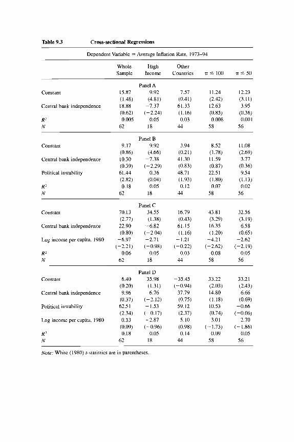
Table 9.3 Cross-sectional Regressions

Dependent Variable = Average Inflation Rate, 1973-94

Whole High Other Sample Income Countries 7~ 5 100 TI 5 50

Panel A Constant 15.87 9.92 7.57 11.24 12.23

(1.48) (4.81) (0.41) (2.42) (3.11) Central bank independence 18.88 -7.37 61.33 12.63 3.95

(0.62) (-2.24) (1.16) (0.85) (0.36) R2 0.005 0.05 0.03 0.008 0.001 N 62 18 44 58 56

Constant 9.17

Central bank independence 10.30

Political instability 61.44

R2 0.18 N 62

(0.86)

(0.39)

(2.82)

Panel B 9.92

(4.66) -7.38 (-2.29)

0.36 (0.04) 0.05

18

3.94 (0.21) 41.30 (0.83) 48.71 ( 1.93) 0.12

44

8.52 (1.78) 11.59 (0.87) 22.51 (1.80) 0.07

58

11.08 (2.69) 3.77

(0.36) 9.54

(1.13) 0.02

56

Constant 70.13

Central bank independence 22.90 (0.80)

Log income per capita, 1980 -6.97 (-2.21)

R2 0.06 N 62

(2.77)

Panel C 34.55 (1.38)

-6.82 (-2.04) -2.71 (-0.98)

0.05 18

16.79 (0.43) 61.15 (1.16)

-1.21 (-0.22)

0.03 44

43.81 (3.29) 16.35 (1.20)

-4.21 (-2.62)

0.08 58

32.56 (3.19) 6.58

(0.65) -2.62

(-2.19) 0.05

56

Constant 6.40 (0.20)

Central bank independence 9.96 (0.37)

Political instability 62.51 (2.34)

Log income per capita, 1980 0.33 (0.09)

RZ 0.18 N 62

Panel D 35.98 (1.31)

-6.76 (-2.12) - 1.53 (-0.17) -2.87 (-0.96)

0.05 18

-35.45 (-0.94)

37.79 (0.75) 59.12 (2.37) 5.10

(0.98) 0.14 44

33.22 (2.03) 14.80 (1.18) 10.53 (0.74)

-3.01 (- 1.73)

0.09 58

33.21 (2.43) 6.66

(0.69) -0.66

(-0.06) -2.70

(-1.86) 0.05

56

Note: White (1980) t-statistics are in parentheses




Whole High Less Sample Income Developed TI 5 100 5 50

Panel A Constant 36.74 7.83 46.67 23.24 18.25

(4.49) (6.14) (4.66) (5.23) (6.56)

(-2.61) (-0.87) (-2.74) (-2.58) (-2.24) Imports/GDP, 1973-94 -0.43 -0.01 -0.55 -0.22 -0.13

R2 0.07 0.004 0.10 0.07 0.05 N 62 18 44 58 56

Constant 137.80 (3.21)

(-3.71)

( - 2.38)

Imports/GDP, 1973-94 -0.66

Log income, 1980 -5.35

RZ 0.15 N 62

Panel B 63.79 (2.87)

-0.18 (-2.78) -2.74

(-2.56) 0.56

18

103.43 (1.62)

-0.67 (-3.37) -3.09 (-0.86)

0.12 44

95.38 7 1.73 (4.55) (4.29)

-0.38 -0.26 (-3.50) (-3.39) -3.82 -2.80 (-3.91) (-3.43)

0.20 0.18 58 56

Constant


Log income, 1980



Log income per capita,

R2 N

1980

76.97 (2.15)

-0.51 (- 3.18) -5.42 (-2.35)

8.46 (0.35) 56.90 (2.24) 5.67

( 1.43) 0.24

62

Panel C -29.75 (-0.56) -0.22

(-3.1 8) -3.30

(-3.13) - 8.02

(-2.00) 35.06 (3.38) 11.78 (1.64) 0.70

18

41.26 (0.85)

-0.78 (-3.03) -6.09 (-1.88) 43.44 (1.07) 42.94 (1.76) 12.33 (2.06) 0.24

44

83.46 (4.05)

-0.38 (-3.15) -4.12 (-3.34)

13.57 (1.15) 9.12

(0.70) 1.40

(0.69) 0.22

58

70.54 (3.61)

-0.27 (-3.03) -3.01 (-2.90)

6.34 (0.69)

-0.62 (-0.06)

0.40 (0.24) 0.19

56

Nore: White (1980) t-statistics are in parentheses

income to the specification; the results on openness remain robust. Thus, our data set also reproduces the basic results about openness.

9.3.2 Basic New Results We now turn to examining the additional issues raised in section 9.2. We

first provide a base case regression and then consider robustness checks. The basic regression contains the following variables: CBI, political insta-

bility, openness, the log level of output, the log level of output per capita, an


exchange-rate-regime dummy (explained below), the average inflation rate during the 1948-72 period, the level of government debt relative to output in 1975, and the grade assigned by Summers and Heston (1988) to the quality of their national accounts data for each country. Several comments about this specification are in order.

The average inflation rate from the presample period is included as a possible measure of the taste for inflation. According to one view, high past inflation implies lower current inflation because countries learn about the costs of inflation and then reform. This implies a negative coefficient. According to a different view, high past inflation leads the economy to invest in technologies for avoiding inflation’s negative effects, which subsequently reduces the costs of inflation. Under this interpretation, the coefficient should be positive. Alter- natively, past inflation might measure persistent aspects of the factors that determine inflation but are unmeasured or poorly measured in our regressions, which again implies a positive coefficient.

We include political instability to proxy a number of possible effects. The most commonly discussed is that more instability makes it difficult for policymakers to commit to low inflation. In addition, countries with political instability probably tend to have larger amounts of underground activity, which raises the optimal inflation rax. Similarly, countries with political instability tend to run inefficient economic programs, which suggests their natural and socially optimal rates of output or unemployment diverge. Nothing in our regressions allows us to sort out these effects, but in each case the expected sign on the coefficient is positive.

We include debt relative to output in 1975 as a measure of the need for tax revenue.’ This variable will not capture all differences in expenditure paths, but the effect of a high initial level of debt on desired tax collections is unam- biguously positive, and this variable is less obviously endogenous with respect to inflation than other possible measures. We show below that other measures, such as expenditure relative to output, produce similar results.

We include the log of income per capita in 1980 to capture several possible effects. A higher level of income per capita is likely to be accompanied by a more sophisticated tax system and a more developed financial system, both of which imply lower optimal inflation tax and thus a negative coefficient. On the other hand, high-income countries might be better at innovating technologies for reducing the costs of inflation, so their inflation aversion might be lower. This implies a positive coefficient.

We include the Summers and Heston quality-of-data score to control for the level of the inflation tax relative to other taxes. For example, countries with large informal sectors, which are typically untaxed, are also likely to have

7. Since we measure inflation over the period 1973-94, it might be preferable to use debt over output in 1973 or 1974. We could not construct this variable for a sufficient number of countries, however.


poor-quality data. The Summers-Heston score is higher for countries with better-quality data, so the coefficient should be negative if the reasoning offered here is correct. This variable might also be correlated with factors that make the socially optimal rate of output or unemployment diverge from the natural rate; again, the expected coefficient is negative.

We include a dummy variable for the kind of exchange rate regime, as in many previous papers, as a further check on the role on the time-consistency considerations. In particular, countries that have agreed to peg their currencies, especially when those agreements involve many countries, may face political costs of excessive inflation and therefore find it relatively easy to maintain a consistent policy. The variable we construct takes a value of 2 for countries that were in multilateral exchange rate systems in 1974, 1 for countries that were in unilateral exchange rate systems, and 0 for countries that allowed their currencies to float. Thus, a higher value of the variable implies, other things equal, a greater commitment to low inflation, so the coefficient should be negative according to the time-consistency hypothesis.

We note that our measure of the exchange rate regime is possibly a poor proxy for any effects of the exchange rate mechanism on inflation. By using data for 1974, we are failing to capture any effects that might have resulted from decisions about the exchange rate regime later in the sample. It is important to avoid using a variable that measures the exchange rate regime during the middle of the sample, however, because such a variable is likely endogenous with respect to inflation. A country might maintain a pegged exchange rate over much or all of a particular sample period because it has solved the time-consistency problem, even if the decision to peg has no marginal effect on its ability to maintain low inflation. Even the variable we construct is problematic, since countries with an underlying distaste for inflation might choose multilateral exchange rate systems consistently, knowing they will have the discipline to live within the implied constraints. The beginning-of-sample measure should be “less endogenous,” however, and we attempt to control for the differences in inflation aversion separately.

This specification omits two key variables. First, we have no direct measure of the discrepancy between the natural rate of output and the socially optimal rate of output. Political instability and quality of the data might capture this effect to some degree, and we attempt more direct measurement below. These attempts are problematic, however, so we omit them from the basic specification. Second, we do not include FOI since it exists only for a narrow sample. Additional results below suggest this omission is not critical.

Table 9.5 presents the main results. CBI enters with the wrong sign in all samples except the high-income sample, and even in this case the coefficient is nowhere near significant. Thus, CBI appears even less reliably related to inflation than indicated by the more parsimonious regressions in table 9.3. The dummy for the exchange rate regime enters with the wrong sign, although not significantly.




Whole High Less Sample Income Developed r 5 100 7~ 5 50

Constant

Average inflation, 1948-72



Impons/GDP, 1973-94

Log income, 1980



Debt/GDP (%), 1975

Quality of the data"

R2 N

- 12.78 (-0.28)

0.59 (1.31) 20.63 (1.32) 60.55 (2.64)

-0.37 (-3.71) -3.87 (-2.52)

12.75 (2.13) 2.58

(1.32) 0.35

(4.98) -5.68 (-2.29)

0.58 49

-92.31 (-1.29)

1.83 (3.63)

-3.45 (-0.71)

21.51 (2.38)

-0.08 (-2.38) -1.12

(-3.00) 15.13 (1.96) 0.77

(0.94) 0.1 1

(3.48) -4.29

(-1.86) 0.87

18

-29.91 (-0.51)

0.59 (1.41) 80.11 (2.47) 49.81 (2.17)

-0.55 (-2.69) -4.14

(-1.75) 14.07 (2.06) 5.50

( 1.69) 0.37

(3.57) -6.33

(-2.61) 0.58

31

16.61 (0.94) 0.25

(1.58) 10.34 (1.15) 7.46

(0.80) -0.30 (-5.33) -2.49 (-2.74)

7.53 (3.65) 0.78

(0.55) 0.23

(4.25) -5.28 (-3.65)

0.55 47

16.61 (0.94) 0.25

(1.58) 10.34 (1.15) 7.46

(0.80) -0.30

(-5.33) -2.49 (-2.74)

7.53 (3.65) 0.78

(0.55) 0.23

(4.25) -5.28

(-3.65) 0.55

47

Nore: White (1980) ?-statistics are in parentheses. 5ummers and Heston 1988.

Political instability enters positively, which is consistent with each of several possible mechanisms, but the result is not overwhelmingly consistent across samples. The magnitude of the estimated effect, however, is large. A one standard-deviation-higher level of political instability is associated with almost a 14.0% higher rate of inflation in the full sample and with a more than 12.0% higher inflation rate in the low-to-moderate-income sample. The estimated effect is essentially zero in the high-income sample, perhaps unsurprisingly.

Past inflation experience is consistently positively associated with current inflation, although the strength of the relation is modest outside the high- income countries. The estimated coefficient in the entire sample is about 0.6, which means 1 percentage-point higher value of prior inflation is associated with more than half a percentage point higher value of current inflation. The estimated effect is more than three times greater in the high-income sample.

The relative strength and magnitude of this relation in the high-income countries might simply indicate that we have failed to capture some determinant of inflation that is especially persistent in the high-income countries. A


more interesting possibility is that high inflation induces investments in technologies for avoiding the costs of inflation. Once these are developed, they are not costly to use, so they reduce future aversion to inflation. The creation or adoption of such technologies might be easier in high-income countries (e.g., they have better-developed financial markets), which would explain the comparative strength of this effect in the high-income countries. The positive relation documented certainly fails to indicate that countries with bad past inflation performances learn from their mistakes and therefore choose lower inflation in the future, other factors held constant.

Openness and the level of income enter both negatively and significantly, although the magnitudes of the estimated effects and their statistical significance fall relative to the more parsimonious regressions in table 9.4. Thus, earlier results appear to have produced estimates of these effects on the high side, but the basic message is robust to controlling for a number of factors not considered in earlier papers. Moreover, the magnitude of the estimated openness effect is still substantial. For the whole sample, the coefficient estimates indicate that a one-standard-deviation-lower import share is associated with an almost 8.0% higher inflation rate. In the high-income sample the estimated effect is only about 1.5%, while in low-to-moderate-income sample it is over 12.0%.

The two variables proxying optimal tax considerations enter consistently with the correct sign and are quite robust: an initially high level of government debt is associated with high future inflation, and countries with lousy data, which we interpret to be countries where collecting revenue via noninflation taxes is difficult, make relatively greater reliance on the inflation tax. These results do not determine whether the inflation tax (and other taxes) are set at exactly the right level given past and future expenditures, nor whether the inflation tax is set exactly right relative to other taxes; in this sense the tests being carried out are far weaker than in the optimal tax literature on the time path of inflation. Nevertheless, the results are consistent with the view that inflation is being used roughly as it should be from an optimal tax perspective.

The magnitudes of these two effects are also substantial. A one-standard- deviation-higher level of the debt-to-income ratio is associated with a more than 8.0% higher inflation rate in the full sample and with a more than 1.5% higher inflation rate in the high-income sample. A one-standard-deviation- higher data-quality score is associated with almost a 9.0% lower rate of inflation using the full sample estimates and with a more than 1.0% lower inflation rate using the high-income sample estimates.

The final result is that, holding constant all the factors discussed, the level of income per capita is consistently positively related to inflation, usually in a robust manner. This outcome suggests the second of the two interpretations offered above, namely, that richer countries adapt to inflation more easily, so their distaste for inflation is lower. The magnitude of the relation is again large: a one-standard-deviation-higher level of income per capita is associated with


approximately a 14.0% higher inflation rate using the full-sample estimates and with an almost 2.0% higher inflation rate using the high-income-sample estimates.

To summarize, the results in table 9.5 suggest that institutional characteristics of an economy, particularly CBI and exchange rate arrangements, are un- important determinants of inflation. Time-consistency issues play a substantial role through the openness mechanism, and possibly through political instability, and optimal tax considerations are critical as well. We now examine whether these conclusions stand up to more rigorous scrutiny.

9.3.3 Robustness Checks As a first check on the robustness of the results presented above, it is useful

to examine the simple correlations between the variables shown in table 9.2. The key fact is that the main results discussed above are present and reasonably robust just in the simple correlations. CBI is positively correlated with inflation in the full sample but negatively correlated in the high-income sample. The exchange rate variable is essentially uncorrelated with inflation in both samples. In most other cases, the signs on the simple correlations are the same as in the multiple regression, and these correlations are often statistically significant.8 The main exception is income per capita. The simple correlation with inflation is negative, but the estimated regression coefficients are always positive. The explanation appears to be that income per capita is positively correlated with a number of other variables, especially the quality-of-data variable.

The next set of checks considers other measures of the taste for inflation. One possibility is that high inflation plays an important role in shaping the tastes for inflation only when past inflation is extreme in some manner. As one check on this possibility, we include the standard deviation of past inflation as an explanatory variable in addition to the mean of past inflation. In all cases, this variable enters negatively, with a t-statistic between 1.0 and 1.5, and the other coefficients are not strongly affected. Thus, this specification provides mild evidence that countries reform in response to past rni~takes.~

A third set of checks concerns our measure of the need for tax revenue. Instead of using the initial level of government debt relative to output, we include the average level of government expenditure relative to output over the 1973-94 period. The results from this specification are consistent with those in table 9.5; expenditure over output always enters positively, although the statistical significance is not overwhelming. When we include both expenditure over output and initial debt relative to output, debt enters positively and robustly while expenditure tends to enter positively but not significantly.

We have also considered a number of alternatives to the Summers-Heston quality-of-data variable as an indicator of countries’ ability to raise noninfla-

8. The calculations of the t-statistics follow Bickel and Doksum 1977, 220-21. 9. All the additional results summarized in this section are available on request from the authors.


tion tax revenue. These include the share of agriculture in GDP, the infant mortality rate, and the high school enrollment rate. None of these variables enters in a robust manner, but the coefficients on all the remaining variables are not particularly sensitive to treatment of this issue.

We have not pursued one further approach to examining this effect, which would consist of estimating the interest elasticity of money demand for each country and including that as a regressor. Such a variable is problematic for our purposes since the estimated elasticity in a particular country in a given time period is likely a function of that country’s inflation rate. This problem is small if the estimated elasticities are approximately equal to the underlying structural parameter, but this condition seems unlikely to hold in practice. The elasticities might be relatively free of this bias if they were estimated for sample periods that do not overlap with our inflation rate sample period, but we do not have the necessary data for the appropriate time periods for a sufficiently large sample of countries.

Our fifth set of robustness checks attempts to measure more directly the gap between the socially optimal rate of outputhnemployment and the noninflation-accelerating rate of outputhnemployment. One natural measure of this gap is the average level of unemployment, assuming the socially optimal but unobserved rates of outputhnemployment are not systematically related to policies that create divergences between the two rates. Unfortunately, data on unemployment tend to be inconsistent, both over time and across countries, so we can construct this variable for a relatively limited set of countries. In this set, the variable enters negatively, contrary to the implications of the time- consistency models, but the relation is weak. In the high-income countries, the estimated relation is positive, although again weak.

As a second way to measure the degree to which policymakers other than the central bank have given the central bank an incentive to raise output, we add the level of government consumption relative to output, with and without the square of this variable. Assuming such consumption increases economic efficiency up to a point but decreases it thereafter, the expected effect on inflation is positive according to the time-consistency models. In both specifications, however, we fail to find a significant effect, and the sign of the estimated effect is sometimes negative.

An issue related to our estimated standard errors is that some observations might be correlated cross-sectionally, perhaps through common involvement in a given exchange rate mechanism or perhaps because geographic proximity produces common susceptibility to certain kinds of shocks. As a crude attempt to address this issue, we reestimated the basic specification including dummy variables for geographic regions.I0 This modification has almost no effect on the results in the full sample. It does lead to significant changes in the high-

10. We included dummies for Africa, Asia, Europe, North and Central America, and South America, and omitted Oceania.


income sample, but these should be discounted since they are based on a regression with only three degrees of freedom.

The fact that we employ a different measure of CBI than in the papers by Romer and Lane raises the question of whether this decision plays a role in the results. We have also estimated the basic specification with the measure used by Romer and Lane, which includes information on actual rates of turnover in central bank governor. This modification has no substantive effect on the results.

One hypothesis we have not examined above is that supply shocks produce inflation differentially across countries. We consider this hypothesis by adding oil imports as a share of output to the basic regression. This variable enters positively in all samples, and the relation is strong (t-statistic of 2.8) for the high-income sample. The remaining coefficients are not affected to any substantial degree by the addition of this variable. Thus, our evidence does suggest that supply shocks play a nonnegligible role, especially in the high-income countries.

The final issue we address is Posen’s measure of FOI. This variable exists for only a subset of countries (roughly, those with inflation rates below 30% during the 1960-89 period), so we cannot add it to all of our specifications. When we add it to our basic regression estimated on Posen’s low-to-moderate inflation sample, however, it enters insignificantly and with a much smaller coefficient than in his results. This is probably not because our additional variables knock it out. Instead, it appears that FOI is only moderately related to inflation even in Posen’s data for the 1970s and 1980s; much of the strength in his results derives from the data for the 1960s.

As a final result, it is useful to consider one further specification. In this regression, we drop CBI, since it does not appear to play an important role and since it is the variable that limits our sample most significantly. This specification provides results for a sample of sixty-eight countries that is almost identi- cal to that for the narrower sample for which CBI exists. Thus, the basic rela- tions documented above appear to exist more broadly.

9.4 Conclusions

The results presented in this paper must be taken with a certain number of grains of salt. Even in the best case, we do not have an enormous number of observations, and in many cases this problem is severe. Many of the proxies we employ are crude, to say the least, and some are potentially endogenous with respect to inflation. The earlier papers in this literature are subject to more or less the same critiques, but caution is nevertheless in order.

Subject to these caveats, our results shed new light on the cross-country determinants of inflation. The more modest conclusions concern the two main hypotheses examined in earlier papers. These papers suggested that CBI is not a substantial causal factor in inflation performance, but our results make this


conclusion inescapable. Conversely, earlier papers made a strong case that openness causes low inflation, and our results help eliminate any residual doubt.

The more interesting results in the paper concern the new issues addressed. We find some evidence that prior inflation experience plays a nonneglible role in inflation performance. The most interesting interpretation is that high inflation produces investments in inflation-avoiding technologies, which then reduce the costs of inflation. The fact that higher income tends to predict higher inflation is consistent with this interpretation. We recognize, however, that other interpretations are possible.

We also find consistent evidence that optimal tax considerations do matter in determining inflation rates. This is perhaps not surprising, since this result is implied by a broad class of models and has been documented in the cases of particular countries. But the result has not previously been demonstrated to hold as widely as found here, and we show both that the overall need for revenue matters and that inflation is adjusted relative to other taxes in the right direction, given the need for revenue.

Our overall summary of these results is that institutional arrangements do not by themselves seem to be of much help in achieving low inflation. Eco- nomic fundamentals, such as openness, political instability, and tax policy, seem to play a much larger role. This does not mean policymakers should ignore institutions or that institutions play no role; our work might simply have little power to demonstrate the importance of institutions or to isolate the critical aspects of institutional arrangements. Nevertheless, our results suggest that quick fixes-increasing the tenure of the central bank governor-do not make a big difference unless the underlying conditions for low inflation are present. Creating those conditions is undoubtedly difficult, but it also appears to be es- sential.

References

Alesina, Alberto, and Lawrence H. Summers. 1993. Central Bank Independence and Macroeconomic Performance: Some Comparative Evidence. Journal of Money, Credit, and Banking (May): 151-62.

Ball, Laurence, and Stephen G. Cecchitti. 1990. Inflation Uncertainty at Long and Short Horizons. Brookings Papers on Economic Activity 1:215-54.

Barro, Robert J. 1991. Economic Growth in a Cross Section of Countries. Quarterly Journal of Economics 106:407-43.

Barro, Robert J., and David B. Gordon. 1983. A Positive Theory of Monetary Policy in a Natural Rate Model. Journal of Political Economy 91589-610.

Bickel, Peter J., and Kjell A. Doksum. 1977. Mathematical Statistics: Basic Ideas and Selected Topics. Oakland, CA: Holden-Day.

Cukierman, Alex, Sebastian Edwards, and Guido Tabellini. 1992. Seigniorage and Po- litical Instability. American Economic Review 82537-55.


Cukierman, Alex, Steven B. Webb, and Bilin Neyapti. 1992. Measuring the Indepen- dence of Central Banks and Its Effect on Policy Outcomes. World Bank Economic Review 6, no. 3: 353-98.

Grilli, Vittorio, Donato Masciandaro, and Guido Tabellini. 1991. Political and Mone- tary Institutions and Public Financial Policies in the Industrial Countries. Economic Policy 13:341-92.

Grilli, Vittorio, and Gian Maria Milesi-Ferretti. 1995. Economic Effects and Structural Determinants of Capital Controls. ZMF StuffPapers 42, no. 3: 517-51.

Kydland, Finn E., and Edward C. Prescott. 1977. Rules Rather Than Discretion: The Inconsistency of Optimal Plans. Journal of Political Economy 85 (June): 473-92.

Lane, Philip. 1995. Inflation in Open Economies. Columbia University. Manuscript. Mankiw, N. Gregory. 1987. The Optimal Collection of Seigniorage: Theory and Evi-

dence. Journal of Monetary Economics 20, no. 2: 327-41. Posen, Adam S. 1993. Why Central Bank Independence Does Not Cause Low Inflation:

The Politics behind the Institutional Fix. Federal Reserve Bank of New York. Manu-

. 1995. Declarations Are Not Enough: Financial Sector Sources of Central Bank Independence. NBER Macroeconomics Annual 10:25 1-74.

Poterba, James, and Julio Rotemberg. 1990. Inflation and Taxation with Optimizing Governments. Journal of Money, Credit, and Banking 22: 1-18.

Rorner, David. 1993. Openness and Inflation: Theory and Evidence. Quarterly Journal of Economics 107, no. 4: 869-903.

Summers, Robert, and Alan Heston. 1988. A New Set of International Comparisons of Real Product and Price Levels Estimates for 130 Countries, 1950-1985. Review of Income and Wealth 34: 1-25.

White, Halbert. 1980. A Heteroskedasticity-Consistent Covariance Matrix Estimator and a Direct Test for Heteroskedasticity. Econometricu 48:817-38.

script.

Comment Maurice Obstfeld

This careful and important paper by Marta Campillo and Jeffrey Miron is the latest to caution against a premature causal interpretation of simple correlations between long-term inflation performance and various measures of central bank independence (CBI). In this spirit, Posen (1995) has argued that CBI and low inflation are both explicable by the effectiveness of the financial communi- ty’s opposition to inflation. The Campillo-Miron study, which systematically assesses an array of potential determinants of inflation for a broad cross-section of countries, suggests that Posen’s empirical results are largely germane to the 1960s. Like Posen, the present authors see little evidence that CBI per se con- tributes to low inflation. Here the factors most robustly and unconditionally correlated with favorable inflation outcomes appear to be low public debt, economic openness, political stability, and quality of aggregate data. Higher past

Maurice Obstfeld is the Class of 1958 Professor of Economics at the University of California,

Research support was provided by the National Science Foundation, the Ford Foundation, and Berkeley, and a research associate of the National Bureau of Economic Research.

the Center for German and European Studies at the University of California, Berkeley.


inflation and higher per capita income appear to aggravate inflation, for reasons that remain unclear.

The authors acknowledge the difficulty of interpreting empirical correlations in the presence of pervasive endogeneity. To address the problem they carry out numerous sensitivity checks, and in their main results often use explanatory variables measured at or close to the start of their sample period, 1973-94. In some cases this choice probably dooms them to finding insignifi- cance.

For example, it is hard to believe that much information about the preferred exchange rate regime is contained in the 1974 observation, drawn from the transitional year between the final Bretton Woods collapse and the Interna- tional Monetary Fund’s formal decision to live without universally fixed exchange rates. On the other hand, the authors are right in their reluctance to use later data. Most satisfactory would be to include as regressors the potential determinants of the exchange rate regime. One of the most important of these, openness, is included and does appear to have a strong negative impact on inflation. One way to assess the channels through which openness discourages inflation would be to study its effect on exchange-rate-regime choice through cross-section regression.

Use of initial (1975) public debt-GDP ratios also appears problematic at first glance, but turns out to be revealing. As figure 9C. 1 shows, many industrial countries have experienced sharp increases in debt-GDP ratios since the early 1970s. (The same statement is true of developing countries.) How much information, then, would one expect to find in data two decades old? Perhaps surprisingly, the answer is, a lot. Figure 9C.2 shows the striking positive correlation between fifteen industrial countries’ debt-GDP ratios in 1975 and in 1991. Least-squares regression yields

Debt,, , R2 = 0.61 _ _ _ = 0.21 + 1.19 __

GDP,, GDP,, (0.07) (0.23)

(with standard errors in parentheses). Interestingly, the high-debt industrial countries of the early 1970s also tended to be the high-debt countries of the early 1990s.

Campillo and Miron interpret the significance of their public-debt variable as evidence of optimal inflation choice, along the lines of Phelps’s extension (1973) of Ramsey taxation to include taxation of money balances. They view their openness, political instability, and data-quality variables as being more directly related to potential dynamic inconsistency in monetary policy, a factor fundamental to the normative case for an independent central bank. However, public debt itself, if denominated in domestic currency, as it generally is, can also be a powerful source of additional inflation credibility problems. I will illustrate the reason at some length, as the point has an important bearing on the lessons to be drawn from this paper’s results.


0.34

0.32

0.3

Z 0.28 IY a 0.26 c3 c3 0.24

Q) 0.22 L3

0.2

0.18

0 .-

2

0.16'1 I I 1 I I I f i I I I 1 I I I 1 1975 1978 1981 1984 1987 1990

Growth in debt, fifteen OECD countries (GDP-weighted average) Fig. 9C.1

1.4

1.2

7 1 Q)

$2 0.8

-- 0.6 Q c

El 0.4 $ 0

a 0.2

-0.2

-0.4

* *

m * *

I * ~

-0.4 -0.2 0 0.2 0.4 0.6 0.8 Debt/GDP in 1975

Fig. 9C.2 Debt ratios, fifteen OECD countries

Consider the following rudimentary model. (See also Calvo 1989.) The government inherits a nominal debt Do contracted at a nominal interest rate of i,, which it must pay off entirely through taxes 7 on nominal output Py and through money creation M - M,, where Mo is the previous period's nominal money stock. After this repayment, the economy comes to an end. The re- sulting government budget constraint is


(1 + i")D, zz P7y + M - M,.

The demand for money in any period is given by the quantity equation M = kPy (notwithstanding the impending end of the economy). If P , denotes the previous period's price level and the inflation rate T is defined as a tax rate on nominal claims,

P - P ,

P ' m = -

then the preceding budget constraint can be reformulated as

Plainly inflation taxes not only real balances ky, but also the real value of the scheduled nominal debt repayment (1 + i,JD,.

Now consider the optimal level of inflation when the government chooses 7 and T according to a Phelpsian optimal tax rule. The government minimizes the loss function

where a measures relative inflation aversion, subject to budget constraint 1. Define the inherited real debt, do = DJP,. The first-order condition for an optimal tax package is

7 4 Tr = -[k + (1 + & - I ,

U Y

which, in combination with constraint 1, yields the government's preferred ex post inflation choice:

(2)

It is easy to see that inflation is an increasing function of the inherited real debt burden, (1 + i,)d,.

The responsiveness of inflation to past debts allows dynamic inconsistency to creep in. If there were no possibility of devaluing the debt ex post through surprise inflation-imagine that all government debt were indexed-then the first-order condition for taxes would be T = rk /a and, assuming the same past real debt do, optimal inflation would be

(1 + i,)d,[k?, + ( 1 + i")d,,I ~-

T = = - - uy' + [ k y + (1 + i,)do]2 '

where r is the (exogenous) real interest rate. But if there is nominal debt, the government will set inflation higher than this level in equilibrium (as one can


show). How high will equilibrium inflation be? Given rational expectations on the part of bondholders, the past nominal interest rate i, fully reflects anticipated future inflation:

l + r

1 - I T 1 + i, =

An equilibrium inflation rate (there may be more than one) is found by substi- tuting this expression into equation 2 and solving for IT. Equilibrium inflation is higher than it would be with indexed debt because, in equilibrium, inflation is anticipated and thus fails to reduce the government’s real interest obligation.

In analogy with the Kydland-Prescott and Barro-Gordon accounts of high- employment monetary policy, inflation expectations raise nominal interest rates and the debt burden, prompting an accommodating monetary response that ultimately is checked by a rising marginal cost of inflation. Not only is inflation higher than it would be with indexed government debt, so are conventional distorting taxes, which also rise to bear part of the increased real debt burden. Thus, the presence of nominal debt creates a classic dynamic inconsistency problem that magnifies the conventional optimal-tax effect of government debt on inflation.

If the Campillo-Miron results on debt levels reflect dynamic inconsistency, rather than a more benign optimal balancing of marginal distortions in a setting of credible policies, then the normative case for CBI certainly is strengthened. Indeed, one potent argument for CBI is that it imposes fiscal discipline by closing off the easy options of money financing and debt devaluation. Thus, an independent central bank may discourage both government debt issue and the ultimate resort to inflationary finance. A world in which CBI affected inflation primarily through this fiscal-discipline channel could yield regression results much like those the authors report. It would be interesting to know if, cross- sectionally, CBI has any impact on fiscal prudence. For industrial countries, casual empiricism indicates a negative answer.

The remarkable positive correlation of debt ratios over time (figure 9C.2) suggests to me instead that political fragmentation and polarization, of the type Roubini and Sachs (1989) link to public deficits, may also help explain long- run inflation performance. Indeed, this is also the main point of Cukierman, Edwards, and Tabellini (1992). Consistent with this view, Posen’s financial opposition to inflation measure ( 1995) includes information on characteristics of the political scene.

The array of unanswered questions does not detract from Campillo and Mir- on’s contribution in investigating a broad range of explanations for inflation within a unified empirical framework. While they rightly view their interpretations as tentative, the patterns they have uncovered provide important starting points for future research. An obvious focus would be the potential casual mechanisms that the authors discuss. Future research should also exploit the


dynamic properties of the data, as in the related study by Grilli and Milesi- Ferretti (1995). One puzzle that might be addressed using time-series data is the following: If public debt, through whatever mechanism, is such an important determinant of inflation, why have inflation rates in the industrial world come down since the early 1980s despite the continuing increase in the average public debt-GDP ratio? And if greater CBI has contributed to this development, can that contribution endure in the absence of parallel fiscal reform?

References

Calvo, Guillermo A. 1989. Controlling Inflation: The Problem of Non-Indexed Debt. In Debt, Adjustment and Recovery: Latin America k Prospect for Growth and Devel- opment, ed. S. Edwards and F. Larrain, 156-75. New York: Blackwell.

Cukierman, Alex, Sebastian Edwards, and Guido Tabellini. 1992. Seigniorage and Po- litical Instability. American Economic Review 82:537-55.

Grilli, Vittorio, and Gian Maria Milesi-Ferretti. 1995. Economic Effects and Structural Determinants of Capital Controls. IMF StaffPapers 42:5 17-5 1.

Phelps, Edmund S. 1973. Inflation in the Theory of Public Finance. Swedish Journal of Economics 75167-82.

Posen, Adam S. 1995. Declarations Are Not Enough: Financial Sector Sources of Cen- tral Bank Independence. NBER Macroeconomics Annual 10:25 1-74.

Roubini, Nouriel, and Jeffrey D. Sachs. 1989. Political and Economic Determinants of Budget Deficits in the Industrial Democracies. European Economic Review 331903-38.

why does inflation differ across countries? · 9 why does inflation differ across countries? marta...

Documents