why do we have an interbank money market?fm · pdf filewhy do we have an interbank money...

Why Do We Have an Interbank Money Market?

Ulrike Neyer∗ Jurgen Wiemers†

Abstract

This paper presents an interbank market model with a heterogeneous banking

sector. We show that banks participate in the interbank market because they

differ in marginal costs of obtaining funds from the European Central Bank.

Our model shows that this heterogeneity implies intermediation by banks

with relatively low marginal costs. The resulting positive spread between the

interbank market rate and the central bank rate is determined by transaction

costs in the interbank market, total liquidity needs of the banking sector, costs

of obtaining funds from the central bank, and the distribution of the latter

across banks.

JEL classification: E43, E52, E58, G21

Keywords: monetary policy, interbank money market, European Central Bank,

monetary policy instruments

∗Martin-Luther-University Halle-Wittenberg, Department of Economics, 06099 Halle/Saale,Germany, Tel.: +49/345/552 33 33, Fax.: +49/345/552 71 90, email: [email protected].

†Halle Institute for Economic Research, P.O. Box 11 03 61, 06017 Halle/Saale, Germany, Tel.:+49/345/77 53 702, Fax.: +49/345/77 53 779, email: [email protected].

We acknowledge the helpful comments of Ulrich Bindseil, Diemo Dietrich, Christian Dreger, HeinzP. Galler, Manfred Jager, Martin Klein, Thomas Linne, Rudiger Pohl, Johannes Stephan andJoachim Wilde.

1

1 Introduction

The interbank money market, and here especially the market for unsecured overnight

loans, plays a crucial role in the conduct of monetary policy. It is the starting point

for the transmission mechanism of monetary policy impulses, and in most industri-

alized countries, the rate on these overnight loans is the central bank’s operating

target. Hence, for the conduct of monetary policy it is important to know the

functioning of this market and the determinants of the interbank money market

rate.

The interbank money market reallocates the liquidity originally supplied by the

central bank. One reason for this reallocation is the offset of anticipated and non-

anticipated daily liquidity imbalances. Furthermore, banks are motivated to parti-

cipate in the interbank market for speculative purposes. With a view on the euro

area, however, we derive an additional reason for the reallocation: a heterogeneous

banking sector. In the euro area, this heterogeneity results from different costs banks

face when borrowing from the central bank. These cost differences occur because

loans from the Eurosystem have to be based on adequate collateral and costs of

holding eligible assets vary across banks within the euro area.

Developing a model which captures this heterogeneity, we show that it induces inter-

mediation. Banks with relatively low marginal costs act as intermediaries between

the central bank and credit institutions with relatively high marginal costs.

Intermediation has important ramifications for the conduct of monetary policy as

the following example shows. The main refinancing operations (MROs) are the

Eurosystem’s key instrument to provide liquidity for the banking sector in the euro

area. They are executed weekly either through a fixed or variable rate tender.1 In the

past, several MROs were characterized by underbidding behaviour2 which led to a

sizeable increase in the interbank money market rate. This underbidding behaviour

occurred when banks expected the central bank to lower interest rates within the

maturity of the respective MRO. The extremely low demand for funds at the central

bank can be attributed to speculation by the banks and to a reduced incentive to

1Some information on the MROs is given in section 2. It should be noted that the Eurosystemdecided on some changes to its operational framework. These changes have been effective sinceMarch 2004. For details concerning these alterations see ECB (2003a, 2003b). For a detaileddescription of the MROs and the other monetary policy instruments of the Eurosystem beforethey were changed see, for example, ECB (2002c). A detailed description of the instrumentsincluding the alterations can be found in ECB (2004a, 2004b).

2A MRO is characterized by underbidding behaviour if the aggregated bidding volume is sig-nificantly below the Eurosystem’s benchmark allotment (for respective literature see page 4). Thebenchmark allotment is the Eurosystem’s assessment of actual liquidity needs of the banking sectorin the euro area, providing smooth provisions of required reserves (see ECB 2002b for details).

2

intermediate. The Eurosystem could have prevented the strong increase in the

interbank market rate by providing the necessary additional liquidity. Typically,

however, the Eurosystem refrained from offsetting the liquidity deficits in order to

drive home the point that underbidding behaviour is a non-profit-making strategy

for the banks (see, for example, ECB 2001a p. 16). This kind of “education” may

work to prevent banks from speculating but it does not help to prevent a reduced

incentive to intermediate. Therefore, if intermediation plays an important role in

the interbank market, this kind of “education” will be fruitless.3

Our model shows that a consequence of the intermediation is a positive spread

between the interbank market rate and the central bank rate. Using data for the

euro area covering the period from January 1999 until December 2003, we test for

a positive spread. The results of our empirical analysis support the outcome of our

model. Furthermore, our theoretical analysis shows that an increase in the central

bank rate leads to a likewise increase in the interbank market rate and that there is a

positive relationship between the total liquidity needs of the banking sector and the

interbank market rate. We test these implications of our model in a cointegration

analysis using data for the euro area. Again we find empirical support for our model.

The bulk of the literature dealing with the interbank money market analyses the

U.S. federal funds market. Developing a model in which individual banks compare

the liquidity benefit of excess reserves with the federal funds rate, Ho and Saunders

(1985) derive different federal funds demand functions and provide several explan-

ations for specific features of the federal funds market. Clouse and Dow (2002)

model the reserve management of a representative bank as a dynamic program-

ming problem capturing main institutional features of the federal funds market to

discuss the effects of various changes to the operating environment and monetary

policy instruments. A large part of the literature which deals with the federal funds

market analyses why the federal funds rate fails to follow a martingale within the

reserve maintenance period, i.e. why banks obviously do not regard reserves held

on different days of the maintenance period as perfect substitutes (see, for example,

Hamilton 1996; Clouse and Dow 1999; Furfine 2000; Bartolini, Bertola, and Prati

2001, 2002a).

However, the results of these papers for the U.S. federal funds market cannot be

easily transferred to the respective markets in other countries because of country

3It should be noted that due to the changes in the Eurosystem’s operational framework (seefootnote 1), the incentives for speculation and a reduced intermediation should not exist anymoresince interest rate changes will not take place during the maturity of a MRO anymore implying thatthe underbidding problem should be solved. For a theoretical analysis concerning the incentiveson behalf of the banks for speculation and a reduced intermediation under the old operationalframework and the non-existing incentives under the new framework see Neyer (2003).

3

specific institutional aspects, as pointed out by Bartolini, Bertola and Prati (2003),

for example. Consequently, papers dealing with liquidity demand and supply in

the euro area consider typical features of the Eurosystem’s operational framework.

Capturing main characteristics of this framework, an extensive number of papers

deals with the causes and consequences of the banks’ under- and overbidding be-

haviour in the MROs (see, for example, Ayuso and Repullo 2001, 2003; Bindseil

2002; Ewerhart 2002; Ewerhart et al 2003; Nautz and Oechssler 2003; and Neyer

2003). Perez-Quiros and Rodrıguez-Mendizabal (2001) construct a model in which

the interest rates of the Eurosystem’s two standing facilities play a crucial role in de-

termining the behaviour of the interbank market rate. Valimaki (2001) presents an

interbank market model to analyse the performance of alternative fixed rate tender

procedures.

Our paper contributes to the existing literature by modelling an interbank money

market which focusses on the following two institutional features in the euro area.

First, contrary to the Federal Reserve System, which provides the liquidity to the

banking sector mainly via outright purchases of securities, the Eurosystem provides

the bulk of liquidity via loans to the banking sector.4 Second, these loans have to be

based on adequate collateral, whereas the costs of holding eligible assets vary across

banks within the euro area.

A close reference to our work is the article by Ayuso and Repullo (2003). Looking

at the euro area, they also find a positive spread between the interbank market

rate and the central bank rate. In their article, the positive spread supports the

hypothesis of an asymmetric objective function of the Eurosystem in the sense that

the Eurosystem, which wants to steer the interbank rate towards a target rate,

is more concerned about letting the interbank rate fall below the target. This

would be consistent with the desire of a young central bank to gain credibility for

its anti-inflationary monetary policy. Ayuso and Repullo focus on the behaviour

of the central bank and its relationship with the credit institutions. Our paper

complements their work by focussing on the behaviour of the credit institutions and

their interrelationship.

The remainder of this paper is structured as follows. Section 2 provides some insti-

tutional background on the money market in the euro area. In section 3 we present

an interbank money market model with a heterogeneous banking sector. Section

4 empirically tests the implications of the model for the euro area, and section 5

summarizes the paper.

4For a detailed comparison of the Eurosystem’s and the Federal Reserve System’s operationalframeworks see, for example, Ruckriegel and Seitz 2002. Bartolini and Prati (2003), also comparingthe two central banks, focus on the different approaches to the execution of the monetary policy.

4

2 Institutional Background

Liquidity Demand

In the euro area, liquidity needs of the banking sector mainly arise from two factors:

the so-called autonomous factors, as banknotes in circulation and government de-

posits with the Eurosystem, and minimum reserve requirements. The Eurosystem’s

minimum reserve system requires credit institutions to hold a fixed amount of com-

pulsory deposits on the accounts with the Eurosystem. These holdings of required

reserves are remunerated close to the market rate.5 In order to fulfil reserve re-

quirements, averaging provisions are allowed over a one-month reserve maintenance

period. Until March 2004, the timing of the reserve maintenance period started

on the 24th calendar day of each month and ended on the 23rd calendar day of

the following month, i.e. it was independent of the dates of the Governing Council

meetings at which interest rate changes were decided. Since March 2004, mainten-

ance periods start on the settlement day of the first MRO following the Governing

Council meetings at which interest rate changes are usually decided, and end on

the day preceding the corresponding settlement day in the following month. The

reason for this change in the timing of the maintenance period has been to avoid

interest rate change speculation within a maintenance period which led to under- or

overbidding behaviour in a couple of MROs.6

Liquidity Supply

The bulk of the liquidity needs of the banking sector (about 74 %) is satisfied by

the Eurosystem through its MROs. About 26 % of the liquidity needs are met

through longer-term refinancing operations, and less than 1 % through fine-tuning

operations. Finally, residual liquidity needs (only about 0.4 %) are balanced by the

banks’ recourse to the marginal lending facilities.7 The MROs, the key instrument of

the Eurosystem to provide the banking sector with liquidity, are credit transactions

which are executed weekly either as a fixed rate or a variable rate tender. From

the launch of the euro in January 1999 until June 2000, tenders were conducted

5See ECB 2004a, p. 58-59 for details.6For a detailed description of the current minimum reserve system we refer the reader to ECB

(2004a), for a description of the reserve system before the changes were effective to ECB (2002c).For details concerning the reason why the Eurosystem has changed its minimum reserve systemsee ECB (2003a).

7For a detailed description of the demand for and the supply of liquidity in the euro area seeECB (2002b). The data given in this paragraph are averages over the period from January 1999until December 2001. Source: ECB (2002b).

5

exclusively as fixed rate tenders. Since then, only variable rate tenders with a

minimum bid rate have been used. With effect from March 2004, the maturity of the

MROs has been reduced from two weeks to one week in order to avoid overlapping

maturities which also induced under- or overbidding behaviour in the MROs in

case of expected interest rate changes.8 The MROs have to be based on adequate

collateral, and although differences in the financial structure across Member States

of the EMU have been considered when defining the list of eligible assets,9 marginal

costs of collateral vary across countries within the euro area (Hamalainen 2000).

Banks also face different costs of holding collateral because they tend to focus on

different business segments. The reason is that as a consequence of this specialization

their asset structures will be distinct from one another, implying that banks have

different marginal opportunity costs of holding eligible collateral.

Reallocation of Liquidity

The liquidity supplied by the Eurosystem is reallocated via the interbank money

market. This market can be divided into the cash market, the market for short-

term securities and the market for derivatives.10 The cash market consists of the

unsecured market, the repo market and the foreign exchange swap market. In the

unsecured market, activity is concentrated on the overnight maturity segment. The

reference rate in this segment is the Eonia (Euro Overnight Index Average). It is

a market index computed as the weighted average of overnight unsecured lending

transactions undertaken by a representative panel of banks. The same panel banks

contributing to the Eonia also quote for the Euribor (Euro Interbank Offered Rate).

The Euribor is the rate at which euro interbank term deposits are offered by one

prime bank to another prime bank. This is the reference rate for maturities of one,

two and three weeks and for twelve maturities from one to twelve months.11 The

market for short term securities includes government securities (Treasury bills) and

private securities (mainly commercial paper and bank certificates of deposits). In

the market for derivatives, typically interest rate swaps and futures are traded.

8For a detailed description of the current design of the MROs we refer the reader to ECB(2004a), for a description of the MROs before the changes were effective to ECB (2002c). Fordetails concerning the reason why the Eurosystem has changed the design of the MROs see ECB(2003a). A theoretical foundation for these alterations can be found in Neyer (2003).

9Eligible assets have been defined by the Eurosystem. For details see ECB (2002c, p. 38-50;2004a, p. 39-54.)

10For more detailed information on the euro money market we refer the reader to ECB (2001b,2002a, 2003b).

11For more information on these reference rates see www.euribor.org.

6

As pointed out in the introduction, institutional features play an important role for

the functioning of the interbank market and therefore for the determinants of the

interbank market rate. The model presented in the following section focusses on two

specific institutional features in the euro area: First, the Eurosystem provides the

bulk of liquidity via loans to the banking sector. Second, these Eurosystem credit

operations have to be based on adequate collateral, and the costs of holding eligible

assets vary across banks within the euro area. We neglect other specific features such

as the kind of the tender procedure the Eurosystem employs to provide the liquidity,

the possibility of averaging provisions of required reserves or the remuneration of

required reserves. Introducing these aspects to the analysis would not change the

main results of our paper but would make the model unnecessarily complex.

3 A Simple Model of an Interbank Money Market

Liquidity Costs and Optimisation

We consider a continuum of measure one of risk-neutral, isolated, price taking banks.

All banks have the same given liquidity needs summarized by the variable R.12 To

cover its liquidity needs, a single bank can borrow liquidity from the central bank

or in the interbank market where it can also place excess liquidity.

The amount bank i borrows from the central bank at a given rate l is denoted

with Ki ≥ 0. This credit transaction with the central bank has to be based on

adequate collateral. We assume that rate of return considerations induce a strict

hierarchy of a bank’s assets,13 and that assets which can serve as collateral have a

relatively low rate of return due to specific criteria they have to fulfil. Consequently,

this collateralization incurs increasing marginal costs. These opportunity costs of

holding collateral are given by

Qi = qiKi + f(Ki), (1)

where f(Ki) ≥ 0, f(0) = 0, f ′ ≥ 0, f ′′ > 0, and f ′(R) < ∞. The bank specific

parameter qi ≥ 0 represents different levels of marginal opportunity costs between

12In our model, the interbank market function of balancing daily liquidity fluctuations couldbe considered by modelling liquidity needs R as a bank-specific random variable or by addingbank-specific shocks. However, this would make the analysis more complicated without changingthe main results of this paper.

13This approach can be compared with the one by Blum and Hellwig (1995). They consider abank with deposits and equity. The bank can put these funds into loans to firms, government bondsor reserves of high powered money. Blum and Hellwig assume that rate of return considerationsinduce a strict preference for loans over bonds and for bonds over reserves.

7

banks (functions, variables, and parameters not indexed by i are the same for each

bank). This heterogeneity in the banking sector is a key feature of our model.

We motivate this heterogeneity by different opportunity costs of holding collateral.

However, there may be other costs in which banks differ when borrowing liquidity

from the central bank, for example, human capital costs.

In the interbank market, a bank can demand liquidity or place excess liquidity. Bank

i’s position in the interbank market is

Bi = R−Ki Q 0. (2)

Trading in the interbank market, the bank faces transaction costs given by

Zi = zh(Bi), (3)

where h(Bi) ≥ 0, h(0) = 0, h′(Bi > 0) > 0, h′(Bi < 0) < 0, h′(0) = 0, h′′(Bi) > 0,

h′(R) < ∞, and the parameter z > 0. Furthermore, we assume the cost function

to be symmetric, i.e. h(Bi) = h(−Bi). This approach of increasing marginal trans-

action costs can be compared with the common method of modelling the liquidity

role of reserves which posits that banks incur increasing costs when liquidity devi-

ates from a target level (see, for example, Campbell 1987; Bartolini, Bertola, and

Prati 2001). The convex form reflects increasing marginal costs of searching for

banks with matching liquidity needs and those resulting from the need to split large

transactions into many small ones to work around credit lines.

Defining l as the interest rate on the central bank credit, and e as the interbank

market rate, bank i’s total liquidity costs are

Ci = Kil + Bie + Qi + Zi. (4)

The first term on the right hand side describes interest payments to the central

bank, the second either interest payments or interest yield from transactions in the

interbank market, and the last two terms represent opportunity costs of holding

collateral and transaction costs. Focussing on prime banks, we neglect any credit

risk in the interbank market. This is in line with the empirical analysis of our model

results, where we use the Eonia and the Euribor as proxy variables for the interbank

market rate. Both the Eonia and the Euribor are computed as the average of the

offer rates of a representative panel of prime banks to other prime banks.

A bank minimizes its total liquidity costs by choosing the optimal level of Ki, subject

to Ki ≥ 0. The first order condition is given by

l + qi + f ′ − e− zh′ = 0. (5)

8

Equation (5) reveals that if a bank covers its liquidity needs at the central bank

and in the interbank market, marginal costs of central bank funds (l + qi + f ′) are

equated to marginal costs of funds borrowed in the interbank market (e + zh′). If a

bank places liquidity in the interbank market, the sum of marginal costs of central

bank funds and marginal transaction costs in the interbank market (l+qi +f ′−zh′)

is equated to marginal revenues in the interbank market e. (Note, that in case the

bank places liquidity in the interbank market h′ < 0 holds.)

Equation (5) implicitly gives the optimal credit demand Kopti (e, l, qi, R, z). Using

the implicit function theorem we find that Kopti,Ki>0 (·) is decreasing in qi:

∂Kopti,Ki>0 (·)∂qi

= − 1

f ′′ + zh′′< 0. (6)

The condition Ki ≥ 0 introduces a non-differentiable point in the partial derivative

∂Kopti /∂qi. We find this point by setting Ki equal to zero and solving equation (5)

for qi. Denoting this upper threshold of qi with q we obtain

q = e− l − f ′(0) + zh′(R). (7)

If qi ≥ q, bank i’s opportunity costs of holding collateral will be so high that it

prefers to cover its total liquidity needs in the interbank market, i.e. Kopti = 0 and

Bi = R.

Evaluating equation (5) at Ki = R and solving for qi, we also find a lower threshold

of qi given by

q = e− l − f ′(R) + zh′(0) = e− l − f ′(R). (8)

If qi < q, bank i’s opportunity costs of holding collateral will be so small that it will

be advantageous to borrow from the central bank to place liquidity in the interbank

market. In this case, the bank will demand more reserves at the central bank than

it actually needs to cover its own requirements, i.e. Kopti > R and Bi < 0. Due

to its relatively low opportunity costs of holding collateral, this bank acts as an

intermediary between the central bank and banks with relatively high opportunity

costs.

Since qi ≥ 0, equation (8) reveals that the interbank market rate must strictly be

greater than the central bank rate (e > l). This result is obvious since otherwise no

bank would be willing to borrow from the central bank to place the liquidity in the

interbank market, i.e. to act as an intermediary. Or to put it differently, no bank

would be interested to act as an intermediary.

9

qiqq

R

Ki

opt

0

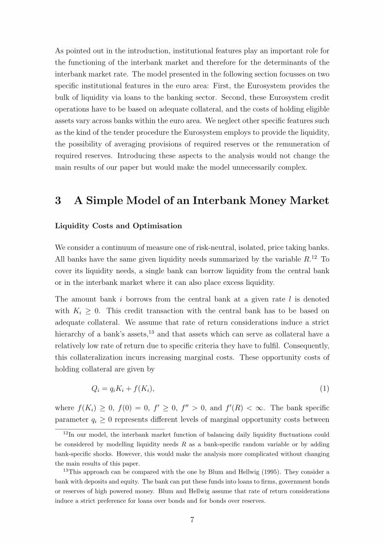
Figure 1: Optimal Credit Demand at the Central Bank

Thus, a bank’s optimal credit demand Kopti (·) is described by the following function:

Kopti (e, l, qi, R) =

Kopti,R≤Ki

(·) if 0 ≤ qi ≤ q

Kopti,0<Ki<R (·) if q < qi < q

0 if q ≤ qi.

(9)

If 0 ≤ qi ≤ q, bank i will demand more reserves at the central bank than it needs

to cover its own liquidity needs, i.e. Kopti > R. If q < qi < q, bank i will cover its

liquidity needs at the central bank and in the interbank market, i.e. 0 < Kopti < R.

Finally, if q ≤ qi, bank i will cover its liquidity needs exclusively in the interbank

market. Figure 1 illustrates this result. It should be noted that the slope of the

curve between 0 and q has been chosen arbitrarily. Its exact shape depends on the

form of the cost functions f(Ki) and h(Bi).

Equilibrium Interbank Market Rate

At the equilibrium interbank market rate e∗, liquidity supply equals liquidity de-

mand. Therefore, assuming that qi is distributed in the interval [0, qmax] across banks

according to the density function g(qi) = G′(qi) with G(0) = 0, e∗ is determined by

q∗∫

0

(Kopti,0≤qi≤q∗(·)−R)g(qi)dqi

=

q∗∫

q∗

[R−Kopti,q∗<qi<q∗(·)]g(qi)dqi +

qmax∫

q∗

Rg(qi)dqi, (10)

10

where q∗ = e∗− l− f ′(R) and q∗ = e∗− l + zh′(R)− f ′(0). The first line of equation

(10) shows liquidity supply in the interbank market, the second liquidity demand.

The demand for liquidity is divided into the demand by credit institutions covering

their liquidity needs partially in the interbank market (first integral) and by banks

covering their total liquidity needs in that market (second integral). Equation (10)

gives us the determinants of e∗ and therefore of the spread (e∗− l): transaction costs

in the interbank market, total liquidity needs of the banking sector, opportunity

costs of holding collateral and the distribution of the latter across banks. Applying

the implicit function theorem we obtain:

∂e∗

∂l= 1 (11)

∂e∗

∂R=

1−q∗∫0

zh′′g(qi)f ′′+zh′′ dqi

q∗∫0

g(qi)f ′′+zh′′dqi

> 0 (12)

∂e∗

∂z=

−q∗∫0

zh′g(qi)f ′′+zh′′dqi

q∗∫0

g(qi)f ′′+zh′′dqi

R 0. (13)

Equation (11) reveals that there is a positive relationship between the interbank

market rate e∗ and the central bank rate l. An increase in l results in increasing

marginal costs of borrowing from the central bank implying that both, in the inter-

bank market supplying and borrowing banks, reduce their demand for funds at the

central bank. Consequently, supply in the interbank market decreases and demand

increases inducing the interbank market rate to rise. Furthermore, equation (11)

shows that a rising l leads to a likewise increase in e∗. The reason is that an increase

in e has the same absolute effect on total marginal liquidity costs as an increase

in l, but in the opposite direction (see the first order condition given by equation

(5)). This means that no wedge is driven between marginal interest payments to

the central bank and marginal interest payments/revenues in the interbank market.

Equation (12) shows that there is also a positive relationship between the interbank

market rate e∗ and total liquidity needs R.14 This result is driven by the cost

functions f(Ki) and h(Bi). If both cost functions are convex, as assumed, it is

obvious that the liquidity supplying banks will cover their additional liquidity needs

by reducing their supply in the interbank market and by demanding more funds at

the central bank, while the banks on the demand side in the interbank market will

14The cost functions h(Bi) and f(Ki) are assumed to be strictly convex, i. e. 0 < zh′′/(f ′′ +zh′′) < 1. This implies that

∫ q∗

0zh′′g (qi) / (f ′′ + zh′′) dqi < 1.

11

cover their additional needs by demanding more funds in the interbank market and

at the central bank.15 Consequently, in the interbank market, the supply decreases

and the demand increases implying a rising interbank market rate.

However, it should be noted that the convexity of both cost functions, f and h, is

not a necessary condition for the result ∂e∗/∂R > 0. This result also holds if only

one cost function is convex and the other is linear, and it may also hold if one is

convex and the other is concave. In the latter case, we additionally have to assume

that the second order condition for a cost minimum, f ′′+zh′′ > 0, is fulfilled. In the

following, we briefly describe the effects of a rising R on e∗ in case one cost function

is assumed to be concave.

If f ′′ < 0 and h′′ > 0 assuming |f ′′| < zh′′, then ∂e∗/∂R R 0, i.e. in case of

decreasing marginal costs of borrowing from the central bank, the interbank market

rate may decrease as a result of rising liquidity needs. The reason is that it may be

advantageous to the supplying banks to demand more funds at the central bank to

place even more liquidity in the interbank market and to the demanding banks to

cover a higher portion of their liquidity needs at the central bank. This would lead

to a decreasing demand and an increasing supply in the interbank market implying

the interbank market rate to fall. Whether this case occurs depends on the increase

of the marginal cost curve h′ relative to the decrease of the marginal cost curve f ′

as well as the density function g(qi).

If h′′ < 0 and f ′′ > 0 assuming that |zh′′| < f ′′, then ∂e∗/∂R > 0, i.e. the effect of

a rising R on e∗ is unambiguously positive. The intuition behind this result is that

it is advantageous to the demanding banks to cover an even higher portion of their

liquidity needs in the interbank market. For the supplying banks marginal costs

of placing liquidity in the interbank market increase since they must demand more

funds at the central bank if they want to maintain their supply in the interbank

market due to their own increased liquidity needs. But borrowing more funds at the

central bank implies increasing marginal costs. As a consequence, banks will reduce

their supply in the interbank market. Therefore, there is an increasing demand and

a decreasing supply leading to a rise in e∗.

The effect of transaction costs on the interbank market rate is ambiguous (see equa-

tion (13)).16 Rising transaction costs in the interbank market imply increasing

marginal costs for both, in the interbank market borrowing and supplying banks.

Consequently, demand as well as supply will fall. It depends on the shape of the cost

15Formally, one obtains this result by using equation (5) and employing the implicit functiontheorem which reveals that ∂Kopt

i /∂R < 1.16Note that for 0 ≤ qi < q∗, h′ < 0 and for q∗ < qi < q∗, h′ > 0.

12

functions f(Ki) and h(Bi) and on the density function g(pi) which effect outweighs

the other and thus whether there is a decrease or increase in e.

The main findings of this section are summarized by the following result:

Result: If opportunity costs of collateral, which banks need to hold to obtain funds

from the central bank, differ between banks, an interbank market will emerge. Banks

with relatively low opportunity costs will act as intermediaries between the central

bank and banks with relatively high costs. The interbank market rate will be higher

than the central bank rate, with the difference being determined by total liquidity

needs of the banking sector, transaction costs in the interbank market, opportunity

costs of holding collateral, and the distribution of the latter across banks.

Illustration

In order to illustrate our results graphically, we postulate the cost functions to be

quadratic:

Qi = qiKi +s

2K2

i (14)

and

Zi =z

2B2

i (15)

with the parameters s, z > 0. Furthermore, we assume a uniform distribution of

qi, with g(qi) = 1. Under these assumptions, Figure 2 shows the interbank market

equilibrium. In panel (a), the upwards sloping curves represent marginal costs of

borrowing from the central bank given by

MCCBi = l + qi + sKi. (16)

Since there is a continuum of banks differing in qi, which is distributed in the interval

[0, qmax], there is a continuum of marginal cost curves between l and (l + qmax). The

downwards sloping curve represents marginal costs of borrowing in the interbank

market. For banks placing liquidity in that market this curve depicts net marginal

revenues (interest yield on interbank loans minus transaction costs). These marginal

costs and revenues are given by

MCIB = MRIB = e + z(R−Ki). (17)

Looking at panel (a) and comparing marginal costs of borrowing from the central

bank with those of borrowing in the interbank market and with marginal revenues

13

MC , MC , MRi

CB IB IB

Ki

l+qmax

l+q

l+q

lR K

max

e*

Bi0R-Kmax

R

qi

qmax

q

q

(a) (b)

MC , MRIB IB

MC |q =q( )i i max

CB

MC |q =q( )i i

CB

MC |q =q( )i i

CB

MC |q =( 0)i i

CB

0

Figure 2: Interbank Market Equilibrium

from placing liquidity in the interbank market respectively, leads to the following

results: For banks with qi > q marginal costs of borrowing from the central bank

are always higher than those of borrowing in the interbank market. Consequently,

Kopti,qi≥q = 0 (we break ties in favour of borrowing in the interbank market). Banks

with q > qi > q partially cover their liquidity requirements at the central bank and

in the interbank market, i.e. 0 < Kopti,q>qi>q < R. The bank-specific amount Kopt

i,q>qi>q

is found at the point where the bank-specific marginal cost curve (MCCBi |q > qi > q)

and the marginal cost curve MCIB intersect. Credit institutions with qi < q borrow

more reserves than they need to cover their own liquidity needs to place the excess

liquidity in the interbank market, i.e. Kopti,qi<q > R. The bank-specific amount

Kopti,qi<q is determined by the intersection of the bank-specific marginal cost curve

(MCCBi |qi < q) and the marginal revenue curve MRIB. Kmax denotes the central

bank credit amount of the bank with the lowest level of marginal opportunity costs

of holding collateral, i.e. with qi = 0.

Panel (b) in Figure 2 represents aggregate demand and supply in the interbank

market. The shaded area to the left of the vertical qi-axis represents aggregate

supply, the respective area to the right aggregate demand. In equilibrium, both

areas have to be of the same size. The equilibrium interbank rate e∗ is determined

by the intersection of the specific marginal cost curve (MCCBi |qi = q) and the

marginal cost/revenue curve (MCIB = MRIB), i.e. where Kopti = R (see equation

17 and replace Ki by R).

Figure 3 illustrates the consequences of an increase in the central bank rate l, li-

quidity needs R, and transaction costs z on liquidity demand and supply in the

14

(a) (c)(b)

qiqi qi

Bi Bi Bi000

q0

q1

q0

qmax

q1

( )R-Kmax

0( )R-K

max

1( )R-K

max

0 ( )R-Kmax

1( )R-K

max

1( )R-Kmax

0R R

0R

q0

q0

q1

qmax

q1

R1

qmax

q0=q1

q0

q1

Increase in l Increase in R Increase in z

A

B

C

D D C

B

A

A B

CD

Figure 3: Comparative Static Analysis

interbank market. The index 0 (1) marks variables before (after) the increase in l,

R and z.

An increase in l implies that in Figure 2 the continuum of the marginal cost curves

MCCBi shifts parallel upwards. The consequent decrease in Kmax, q and q implies

that in Figure 3, panel (a) aggregate supply shrinks from the area (A+B) to the

triangle B. Aggregate demand, on the other hand, increases from the area D to the

area (C+D). Consequently, there will be a rise in e to restore market equilibrium.

Graphically, this rise in e shifts the marginal cost/revenue curve (MCIB = MRIB)

upwards, implying Kmax, q and q to increase again, until the areas to both sides of

the vertical qi-axis are of the same size again.

In Figure 2, an increase in R leads to a parallel upward shift of the marginal

cost/revenue curve (MCIB = MRIB). Furthermore, on the horizontal axis, R moves

to the right. The shift of the marginal cost/revenue curve implies Kmax to increase,

but since this increase must be smaller than the rise in R (∂Kopti /∂R < 1) the dis-

tance RKmax becomes smaller which implies that q decreases. The upper threshold

q, on the other hand, increases. Therefore, as Figure 3, panel (b) illustrates, aggreg-

ate supply shrinks from the area (A+B) to B, whereas aggregate demand increases

from the area D to (D+C). Hence, the interbank market rate e will rise to restore

the market equilibrium.

In Figure 2, an increase in z implies the marginal cost/revenue curve (MCIB =

MRIB) to turn clockwise in that point where it intersects with the marginal cost

curve (MCCBi |qi = q) (a change in z does not imply a change in q as long as e

has not changed yet, see equation (8)). Therefore, the marginal cost/revenue curve

becomes steeper implying q to rise and Kmax to fall. Consequently, as Figure 3

shows, aggregate demand and supply shrink such that the effect on e∗ is ambiguous.

15

4 Empirical Analysis

Money Market Rate and ECB Rate: Test of the Spread

The purpose of our paper is to show that intermediation occurs due to cost differ-

ences between banks in obtaining funds from the central bank. Looking at the euro

area, one obtains the most obvious indication of intermediation when considering

that only a small fraction of all banks actually takes part in the MROs.17 A further

indication would be an on average positive spread between the interbank market

rate and the rate banks have to pay at the central bank. The following empirical

analysis shows that the spread is significantly positive.

The spread between the interbank market rate and the central bank rate has been

examined in a number of recent publications (see, for example, Ayuso and Repullo

2003; Ejerskov, Moss, and Stracca 2003; Nyborg, Bindseil, and Strebulaev 2002).

While the positive sign of the spread is not explicitly tested in the latter two pub-

lications, Ayuso and Repullo do find a significantly positive spread. Our test differs

from Ayuso and Repullo’s in the interest rates used to approximate the interbank

market rate and the central bank rate as well as in the samples used for the analysis.

Testing for a positive spread, Ayuso and Repullo use two alternative measures of the

interbank market rate, namely the Eonia and the one-week Euribor. As a proxy for

the central bank rate, they employ the fixed rate applied to the fixed rate tenders

and the minimum bid rate of the variable rate tenders. Additionally, we test for a

positive spread between the two-week Euribor (which has not been available for the

sample period used by Ayuso and Repullo) and the weighted average rate of the

variable rate tenders. The advantage of testing for a positive spread between these

two rates is that the maturities of the underlying credit transactions are identical.

Furthermore, the weighted average rate of the variable rate tenders is a more appro-

priate rate for comparing the actual liquidity costs when borrowing in the interbank

market with those when borrowing from the central bank which is a key issue of our

model.

We start our analysis by comparing the key central bank rate in the euro area,

i.e. the fixed rate applied to the fixed rate tenders and the minimum bid rate of the

variable rate tenders, with the key interbank money market rate, i.e. the Eonia. Our

17At the end of 2000 (Junes 2003), the criteria for participating in the MROs were fulfilled by2542 (2242) credit institutions (ECB 2001c, p. 63, ECB 2004b, p. 75). But in 1999 and 2000 thetotal number of institutions which actually took part in these operations fluctuated between 400and 600. Also in 2001 and 2002 the number of banks taking part in the MROs was relatively small:it fluctuated between 175 and 658, on average 357 banks took part in the MROs. In the first halfof 2003, the total number of counterparties participating in the MROs averaged 253 institutions.

16

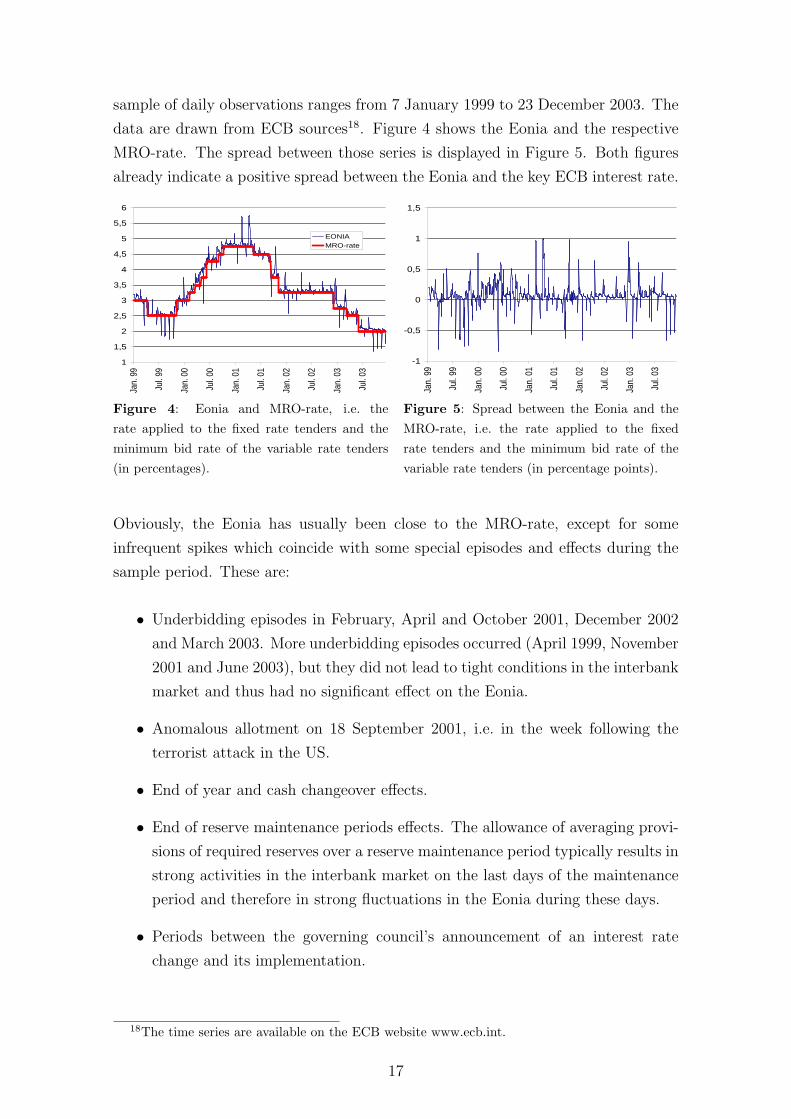
sample of daily observations ranges from 7 January 1999 to 23 December 2003. The

data are drawn from ECB sources18. Figure 4 shows the Eonia and the respective

MRO-rate. The spread between those series is displayed in Figure 5. Both figures

already indicate a positive spread between the Eonia and the key ECB interest rate.

1

1,5

2

2,5

3

3,5

4

4,5

5

5,5

6

Jan.

99

Jul.

99

Jan.

00

Jul.

00

Jan.

01

Jul.

01

Jan.

02

Jul.

02

Jan.

03

Jul.

03

EONIAMRO-rate

Figure 4: Eonia and MRO-rate, i.e. therate applied to the fixed rate tenders and theminimum bid rate of the variable rate tenders(in percentages).

-1

-0,5

0

0,5

1

1,5

Jan.

99

Jul.

99

Jan.

00

Jul.

00

Jan.

01

Jul.

01

Jan.

02

Jul.

02

Jan.

03

Jul.

03

Figure 5: Spread between the Eonia and theMRO-rate, i.e. the rate applied to the fixedrate tenders and the minimum bid rate of thevariable rate tenders (in percentage points).

Obviously, the Eonia has usually been close to the MRO-rate, except for some

infrequent spikes which coincide with some special episodes and effects during the

sample period. These are:

• Underbidding episodes in February, April and October 2001, December 2002

and March 2003. More underbidding episodes occurred (April 1999, November

2001 and June 2003), but they did not lead to tight conditions in the interbank

market and thus had no significant effect on the Eonia.

• Anomalous allotment on 18 September 2001, i.e. in the week following the

terrorist attack in the US.

• End of year and cash changeover effects.

• End of reserve maintenance periods effects. The allowance of averaging provi-

sions of required reserves over a reserve maintenance period typically results in

strong activities in the interbank market on the last days of the maintenance

period and therefore in strong fluctuations in the Eonia during these days.

• Periods between the governing council’s announcement of an interest rate

change and its implementation.

18The time series are available on the ECB website www.ecb.int.

17

In order to test for a positive spread, we exclude these periods from the sample

because we aim to test the positive sign of the spread under “normal” conditions.

Furthermore, since we use weekly data for the tests of the Euribor spreads below, we

also use weekly data for the Eonia spread to make results comparable.19 The first

column of Table 1 reports the one-sided test of the null hypothesis of a non-positive

spread against the alternative of a positive spread between the Eonia and the MRO-

rate. The average spread was 10.5 basis points during the fixed tender period and

fell to 6.1 basis points during the variable tender period. The null hypothesis of a

non-positive spread can be rejected on a confidence level of 1%.

However, this test involves two potential biases that might affect the spread. First,

the MROs have a two-week maturity20 which implies that the MRO-rate has a

positive term premium when compared to the Eonia which in turn refers to overnight

transactions. This should bias the spread downwards. Second, differences in credit

risk may bias the spread upwards since the MROs are collateralized while the Eonia

refers to unsecured interbank market transactions.21 In order to reduce the first bias,

we use the two-week Euribor for testing whether the spread is positive. The two-week

Euribor has the same maturity as the MROs, thus the term premiums should be

equal. Due to the fact that the two-week Euribor is available only since 15 October

2001, we also use the one-week Euribor, which is already available since January

1999, providing us with a much larger sample while the difference in maturity is

only one week.22 The second bias should generally be small since the Eonia and

the Euribor are only offered to banks of first class credit standing. Additionally,

we do not compare the respective Euribor with the minimum bid rate but with the

weighted average rate during the variable rate tender period. The reason is that

the latter is a more appropriate rate when comparing the actual liquidity costs in

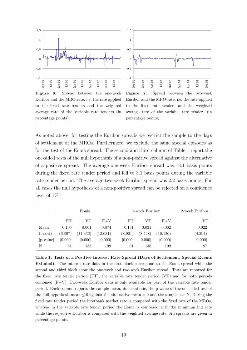
the interbank market with those at the central bank. Figures 6 and 7 show daily

data on the one-week and two-week Euribor spreads. Both figures already indicate

an on average positive spread between the respective interbank market rate and the

respective central bank rate.

19We use weekly data for testing the Euribor spreads to ensure that the maturity of the re-spective interbank term deposits is as long as the maturity of the respective MRO.

20Note, that since March 2004, which is outside our sample period, the MROs have a maturityof one week.

21Concerning a discussion of these two potential biases see also Ayuso and Repullo (2003).22The data on the one-week and two-week Euribor is available on www.euribor.org.

18

-1

-0,5

0

0,5

1

1,5

Jan.

99

Jul.

99

Jan.

00

Jul.

00

Jan.

01

Jul.

01

Jan.

02

Jul.

02

Jan.

03

Jul.

03

Figure 6: Spread between the one-weekEuribor and the MRO-rate, i.e. the rate appliedto the fixed rate tenders and the weightedaverage rate of the variable rate tenders (inpercentage points).

-1

-0,5

0

0,5

1

1,5

Okt

. 01

Jan.

02

Apr.

02

Jul.

02

Okt

. 02

Jan.

03

Apr.

03

Jul.

03

Okt

. 03

Figure 7: Spread between the two-weekEuribor and the MRO-rate, i.e. the rate appliedto the fixed rate tenders and the weightedaverage rate of the variable rate tenders (inpercentage points).

As noted above, for testing the Euribor spreads we restrict the sample to the days

of settlement of the MROs. Furthermore, we exclude the same special episodes as

for the test of the Eonia spread. The second and third column of Table 1 report the

one-sided tests of the null hypothesis of a non-positive spread against the alternative

of a positive spread. The average one-week Euribor spread was 13.1 basis points

during the fixed rate tender period and fell to 3.1 basis points during the variable

rate tender period. The average two-week Euribor spread was 2.2 basis points. For

all cases the null hypothesis of a non-positive spread can be rejected on a confidence

level of 1%.

Eonia 1-week Euribor 2-week Euribor

FT VT F+V FT VT F+V VT

Mean 0.105 0.061 0.074 0.131 0.031 0.062 0.022(t-stat) (6.807) (11.336) (12.031) (8.901) (8.448) (10.126) (4.394)[p-value] [0.000] [0.000] [0.000] [0.000] [0.000] [0.000] [0.000]N 61 138 199 61 138 199 87

Table 1: Tests of a Positive Interest Rate Spread (Days of Settlement, Special Events

Exluded). The interest rate data in the first block correspond to the Eonia spread while thesecond and third block show the one-week and two-week Euribor spread. Tests are reported forthe fixed rate tender period (FT), the variable rate tender period (VT) and for both periodscombined (F+V). Two-week Euribor data is only available for part of the variable rate tenderperiod. Each column reports the sample mean, its t-statistic, the p-value of the one-sided test ofthe null hypothesis mean ≤ 0 against the alternative mean > 0 and the sample size N. During thefixed rate tender period the interbank market rate is compared with the fixed rate of the MROs,whereas in the variable rate tender period the Eonia is compared with the minimum bid ratewhile the respective Euribor is compared with the weighted average rate. All spreads are given inpercentage points.

19

To check for robustness of the spreads, we also tested the Eonia spread and the two

Euribor spreads using daily data, with and without the exclusion of special events.

Results are presented in the appendix. We can also reject the null hypothesis of a

zero spread for all cases on a 1% level.

A Test of the Results of the Comparative Static Analysis

Apart from predicting a positive spread between the interbank market rate and the

central bank rate, the comparative static analysis of the last section shows that

our model also implies qualitative and quantitative relations between the interbank

market rate e and some of its determining variables. Therefore, we also test the result

of our theoretical model that ∂e∗/∂l = 1 and ∂e∗/∂R > 0. The effect of transaction

costs, collateral opportunity costs and the distribution of the latter across banks on

the equilibrium interbank market rate are captured by a constant and, if their effect

changes over time, by including a trend in the following cointegration analysis.

According to standard unit root tests, the one-week Euribor (our proxy for e) and

the MRO rate, i.e. the rate applied to the fixed rate tenders and the weighted average

rate of the variable rate tenders (used for l) are I(1) variables for the whole sample

period ranging from 7 January 1999 to 23 December 2003. Again, all series are

observed on the days of settlement of the tender, which results in a sample size of

T = 259. Figure 8 displays both interest rates. The series of banks’ total liquidity

needs R is the sum of autonomous factors and required reserves.23 Figure 9 shows a

distinct double trend break in R which is mainly due to a large decrease in banknotes

in circulation before the introduction of the Euro money in January 2002 and the

strong rebound since April 2002 (ECB 2004b, p. 89). Allowing for a piecewise linear

trend in the ADF test using bootstrapped critical values, we can reject the unit root

for R on a 10% level.

23The respective time series are available on the ECB website www.ecb.int.

20

1,5

2

2,5

3

3,5

4

4,5

5

Jan.

99

Jul.

99

Jan.

00

Jul.

00

Jan.

01

Jul.

01

Jan.

02

Jul.

02

Jan.

03

Jul.

03

1-week Euribor

MRO-rate

Figure 8: One-week Euribor and the MRO-rate, i.e. the rate applied to the fixed ratetenders and the weighted average rate of thevariable rate tenders (in percentages).

150

200

250

300

Jan.

99

Jul.

99

Jan.

00

Jul.

00

Jan.

01

Jul.

01

Jan.

02

Jul.

02

Jan.

03

Jul.

03

Figure 9: Banks total liquidity needs, i.e.the sum of autonomous factors and requiredreserves (billion Euro).

Since the I(1) hypothesis cannot be rejected for the interest rate variables, we test

for cointegration (Johansen 1988; Johansen 1996). A complication arises from the

inclusion of the double trend break present in R in the cointegration analysis since

the critical values of the rank tests depend on the number and location of break

points and the trend specification. Johansen, Mosconi & Nielsen (2000) propose

a modification of the standard Johansen model which allows for a piecewise linear

trend with known break points. They estimate response surface functions which

allow for computing critical values of the rank statistics, and they develop tests for

changes in the slope parameters of the deterministic trends. These techniques are

implemented in MALCOM (Mosconi 1998) for RATS24, which has been used for

this study.

Following this approach, we divide our sample into three periods j = 1, 2, 3 with

length Tj − Tj−1 (0 = T0 < T1 < T2 < T3 = T ), so that T1 and T2 denote the

respective breakpoints in December 2000 and April 2002, and estimate the model

∆Xt = (Π, Πj)

(Xt−1

t

)+ µj +

k−1∑i=1

Γi∆Xt−i + εt (18)

for j = 1, 2, 3 conditionally on the first k observations of each subsample, where ∆ is

the difference operator, X = (e, l, ln (R))′ is the vector of the endogenous variables

and Π, Πj, Γi, µj are coefficient matrices and vectors. The innovations εt are

assumed to be independently, identically normally distributed with mean zero and

variance Ω. Defining appropriate dummy variables, equations (18) can be written

as one equation, which facilitates estimation with standard econometric software

(Johansen, Mosconi, and Nielsen 2000, p. 29).

24www.estima.com

21

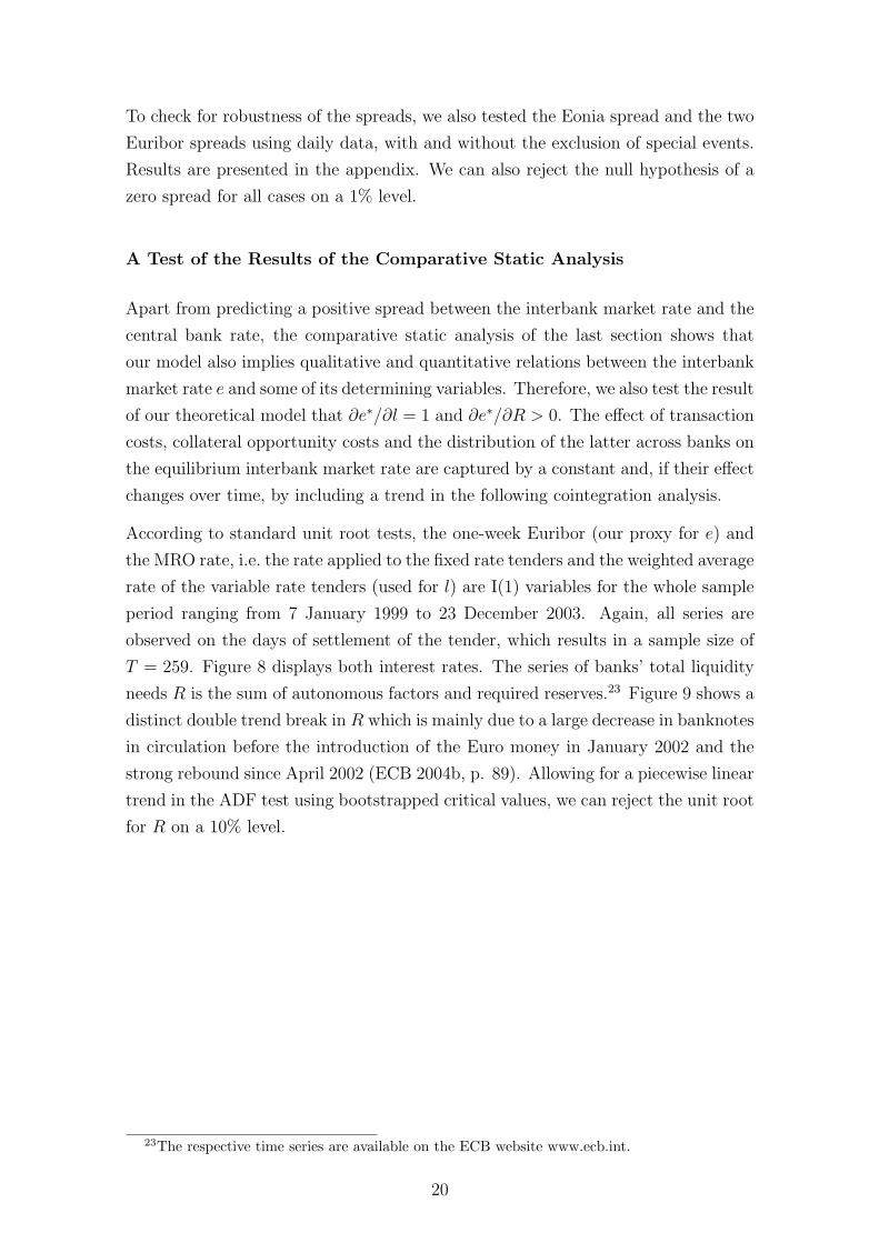
As a first step, we determine the maximum lag k of the vector autoregressive model

(VAR). Table 2 reports information criteria for different values of k and the modified

Godfrey portmanteau test (Sims 1980).

k Akaike Hannan-Quinn Schwartz Godfrey χ2ar5

(45)

1 -16.244 -16.059 -15.784 0.0552 -16.165 -15.896 -15.497 0.0413 -16.088 -15.735 -15.211 0.1614 -16.064 -15.627 -14.977 0.3895 -16.016 -15.495 -14.721 0.517

Table 2: Maximum Lag Analysis: Information Criteria and p-value for the Modified

Godfrey Portmanteau Test.

The information criteria unanimously suggest a lag length of one. Therefore, k = 1

has been selected, since it is also the first lag which gives approximately white

noise, as the Godfrey portmanteau test shows. Conventional diagnostic tests do

not suggest the presence of serial correlation, heteroscedasticity and ARCH effects

in the residuals of the VAR, but the Jarque-Bera tests in Table 3 show that the

normality assumption is strongly violated in our model. Residuals for the interest

rates are skewed and also leptokurtic which is a typical feature of high frequency

financial market data. However, in a comparison of systems cointegration tests,

Hubrich, Lutkepohl & Saikkonen (2001) argue that in the case of a non Gaussian

data generating process the Johansen approach amounts to computing a pseudo

likelihood ratio test which still may have better properties than many competitors.

Equation Skewness Kurtosis Sk+Kur

One-week Euribor 0.000 0.000 0.000MRO-rate (avg) 0.000 0.000 0.000Liquidity requirements 0.048 0.887 0.141

Table 3: Jarque-Bera Normality Tests (p-values).

Cointegration appears if (Π, Πj) in equation (18) has reduced rank so that it can

be written as (Π, Πj) = α (β′, γ′), where α and β are (p× r) matrices and γ is

(1× r) with p = 3. As can be seen from equation (18), we restrict the linear trend

to the cointegration space and thus exclude a quadratic trend in the levels of Xt.

The trace test to determine the cointegration rank is reported in Table 4. The test

suggests a rank of r = 2, which is therefore chosen for the following analysis. Table 5

shows the characteristic roots of the I(0) model (r = 3) and the I(1) model (r = 2),

which corroborate the assumption r = 2. In addition, tests for the stability of the

22

cointegration rank and the cointegration space (Hansen and Johansen 1992) give

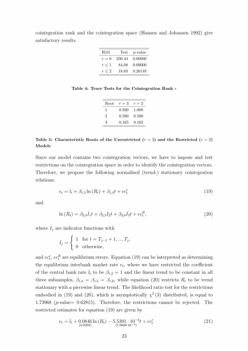
satisfactory results.

H(0) Test p-value

r = 0 230.44 0.00000r ≤ 1 84.08 0.00000r ≤ 2 18.63 0.26148

Table 4: Trace Tests for the Cointegration Rank r

Root r = 3 r = 2

1 0.930 1.0002 0.590 0.5903 0.165 0.162

Table 5: Characteristic Roots of the Unrestricted (r = 3) and the Restricted (r = 2)Models

Since our model contains two cointegration vectors, we have to impose and test

restrictions on the cointegration space in order to identify the cointegration vectors.

Therefore, we propose the following normalised (trend-) stationary cointegration

relations:

et = lt + β1,3 ln (Rt) + β1,4t + ecet (19)

and

ln (Rt) = β2,4I1t + β2,5I2t + β2,6I3t + ecRt , (20)

where Ij are indicator functions with

Ij =

1 for t = Tj−1 + 1, ..., Tj,

0 otherwise,

and ecet , ecR

t are equilibrium errors. Equation (19) can be interpreted as determining

the equilibrium interbank market rate et, where we have restricted the coefficient

of the central bank rate lt to be β1,2 = 1 and the linear trend to be constant in all

three subsamples, β1,4 = β1,5 = β1,6, while equation (20) restricts Rt to be trend

stationary with a piecewise linear trend. The likelihood ratio test for the restrictions

embodied in (19) and (20), which is asymptotically χ2 (3) distributed, is equal to

1.73968 (p-value= 0.62815). Therefore, the restrictions cannot be rejected. The

restricted estimates for equation (19) are given by

et = lt + 0.0846(0.0202)

ln (Rt)− 5.5391 · 10−4

(1.0026·10−4)t + ece

t (21)

23

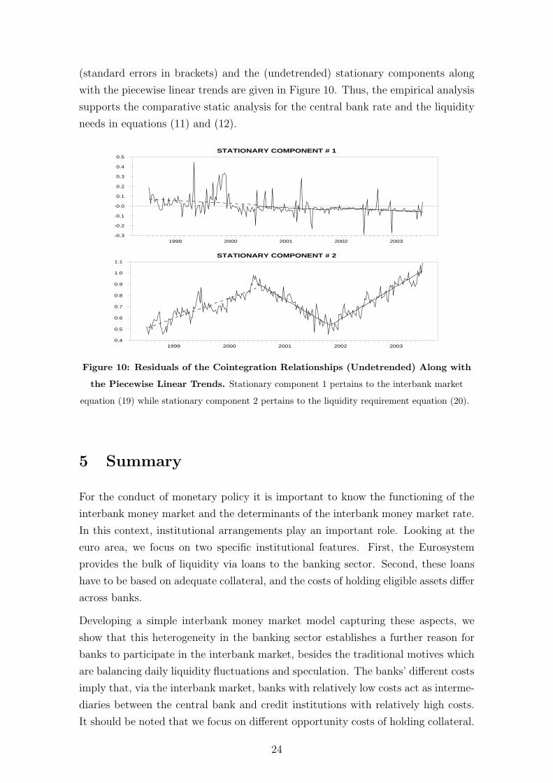
(standard errors in brackets) and the (undetrended) stationary components along

with the piecewise linear trends are given in Figure 10. Thus, the empirical analysis

supports the comparative static analysis for the central bank rate and the liquidity

needs in equations (11) and (12).

STATIONARY COMPONENT # 1

1999 2000 2001 2002 2003-0.3

-0.2

-0.1

-0.0

0.1

0.2

0.3

0.4

0.5

STATIONARY COMPONENT # 2

1999 2000 2001 2002 20030.4

0.5

0.6

0.7

0.8

0.9

1.0

1.1

Figure 10: Residuals of the Cointegration Relationships (Undetrended) Along with

the Piecewise Linear Trends. Stationary component 1 pertains to the interbank market

equation (19) while stationary component 2 pertains to the liquidity requirement equation (20).

5 Summary

For the conduct of monetary policy it is important to know the functioning of the

interbank money market and the determinants of the interbank money market rate.

In this context, institutional arrangements play an important role. Looking at the

euro area, we focus on two specific institutional features. First, the Eurosystem

provides the bulk of liquidity via loans to the banking sector. Second, these loans

have to be based on adequate collateral, and the costs of holding eligible assets differ

across banks.

Developing a simple interbank money market model capturing these aspects, we

show that this heterogeneity in the banking sector establishes a further reason for

banks to participate in the interbank market, besides the traditional motives which

are balancing daily liquidity fluctuations and speculation. The banks’ different costs

imply that, via the interbank market, banks with relatively low costs act as interme-

diaries between the central bank and credit institutions with relatively high costs.

It should be noted that we focus on different opportunity costs of holding collateral.

24

However, the crucial point is that banks differ in costs of obtaining funds from the

central bank, which can also be human capital costs, for example.

Our model shows that a consequence of this intermediation is a positive spread

between the interbank market rate and the central bank rate. Our empirical analysis

strongly supports a positive spread for the euro area.

With the help of our interbank market model, we derive the following determinants of

the interbank market rate: the central bank rate, transaction costs in the interbank

market, total liquidity needs of the banking sector, collateral’s opportunity costs,

and the distribution of the latter across banks. In order to test the comparative

static results of our model we perform a cointegration analysis. We identify a long-

run relationship between the interbank market rate, the central bank rate and the

total liquidity needs of the banking sector. The estimated equation supports our

comparative static results.

References

Ayuso, J., and R. Repullo (2001): “Why Did the Banks Overbid? An Empirical

Model of the Fixed Rate Tenders of the European Central Bank,” Journal of

International Money and Finance, 20, 857–870.

(2003): “A Model of the Open Market Operations of the European Central

Bank,” Economic Journal, 113, 883–902.

Bartolini, L., G. Bertola, and A. Prati (2001): “Banks’ Reserve Man-

agement, Transaction Costs, and the Timing of Federal Reserve Intervention,”

Journal of Banking and Finance, 25, 1287–1317.

(2002): “Day-To-Day Monetary Policy and the Volatility of the Federal

Funds Interest Rate,” Journal of Money, Credit, and Banking, 34, 137–159.

(2003): “The Overnight Interbank Market: Evidence from the G-7 and the

Euro Zone,” Journal of Banking and Finance, 27(10), 2045–2083.

Bartolini, L., and A. Prati (2003): “The Execution of Monetary Policy: A Tale

of Two Central Banks,” Economic Policy, 18(37), 435–467.

Bindseil, U. (2002): “Equilibrium Bidding in the Eurosystem’s Open Market Op-

erations,” European Central Bank Working Paper No. 137.

Blum, J., and M. Hellwig (1995): “The Macroeconomic Implications of Capital

Adequacy Requirements for Banks,” European Economic Review, 39, 739–749.

25

Clouse, J. A., and J. P. Dow Jr. (2002): “A Computational Model of Banks’

Optimal Reserve Management Policy,” Journal of Economic Dynamics and Con-

trol, 26, 1787–1814.

Clouse, J. A., and J. P. Dow Jr. (1999): “Fixed Costs and the Behaviour of

the Federal Funds Rate,” Journal of Banking and Finance, 23, 1015–1029.

Ejerskov, S., C. M. Moss, and L. Stracca (2003): “How Does the ECB Allot

Liquidity in its Weekly Main Refinancing Operations? A Look at the Empirical

Evidence,” European Central Bank Working Paper No. 244.

European Central Bank (2001a): “Economic Developments in the Euro Area,”

ECB Monthly Bulletin, November 2001, pp. 7–38.

(2001b): “The Euro Money Market,” Frankfurt.

(2001c): The Monetary Policy of the ECB. European Central Bank, Frank-

furt.

(2002a): “The Euro Money Market Study 2001 (MOC),” Frankfurt.

(2002b): “The Liquidity Management of the ECB,” ECB Monthly Bulletin,

May 2002, pp. 41–53.

(2002c): The Single Monetary Policy in the Euro Area - General Docu-

mentation on Eurosystem Monetary Policy Instruments and Procedures. European

Central Bank, Frankfurt.

(2003a): “Changes to the Eurosystem’s Operational Framework,” ECB

Monthly Bulletin, August 2003, pp. 41–54.

(2003b): “Measures to Improve the Efficiency of the Operational

Framework for Monetary Policy,” (ECB Press Release, 23 January 2003, see

www.ecb.int).

(2003c): “Money Market Study 2002,” Frankfurt.

(2004a): The Implementation of Monetary Policy in the Euro Area.

European Central Bank, Frankfurt.

(2004b): The Monetary Policy of the ECB. European Central Bank, Frank-

furt.

Ewerhart, C. (2002): “A Model of the Eurosystem’s Operational Framework for

Monetary Policy Implementation,” European Central Bank Working Paper No.

197.

26

Ewerhart, C., N. Cassola, S. Ejerskov, and N. Valla (2003): “Optimal

Allotment Policy in the Eurosystem’s Main Refinancing Operations,” European

Central Bank Working Paper No. 295.

Furfine, C. H. (2000): “Interbank Payments and the Daily Federal Funds Rate,”

Journal of Monetary Economics, 46, 535–553.

Hamalainen, S. (2000): “The Operational Framework of the Eurosystem,”

Welcome address at the ECB Conference on the Operational Framework of

the Eurosystem and the Financial Markets in Frankfurt, 5-6 May 2000, (see

www.ecb.int).

Hamilton, J. D. (1996): “The Daily Market for Federal Funds,” Journal of Polit-

ical Economy, 104, 26–56.

Hansen, H., and S. Johansen (1992): “Recursive Estimation in Cointegrated

VAR-Models,” Discussion papers 92-13, Institute of Economics, University of

Copenhagen.

Ho, T. S. Y., and A. Saunders (1985): “A Micro Model of the Federal Funds

Rate,” Journal of Finance, 40, 977–986.

Hubrich, K., H. Lutkepohl, and P. Saikkonen (2001): “A review of systems

cointegration tests,” Econometric Reviews, 20, 247–318.

Johansen, S. (1988): “Statistical analysis of cointegration vectors,” Journal of

Economic Dynamics and Control, 12, 231–254.

(1996): Likelihood-based inference in Cointegrated Vector Autoregressive

Models. Oxford University Press.

Johansen, S., R. Mosconi, and B. Nielsen (2000): “Cointegration analysis

in the presence of structural breaks in the deterministic trend,” Econometrics

Journal, 3, 216–249.

Mosconi, R. (1998): MALCOM - The theory and practice of cointegration analysis

in RATS. Libreria Editrice Cafoscarina, Milano.

Nautz, D., and J. Oechssler (2003): “The Repo Auctions of the European Cent-

ral Bank and the Vanishing Quota Puzzle,” Scandinavian Journal of Economics,

105, 207–220.

Neyer, U. (2003): “Banks’ Behaviour in the Interbank Market and the Eurosys-

tem’s Operational Framework,” Martin-Luther-University Halle-Wittenberg, De-

partment of Economics, Discussion Paper No. 29. Forthcoming in: European

Review of Economics and Finance.

27

Nyborg, K. G., U. Bindseil, and I. A. Strebulaev (2002): “Bidding and

Performance in Repo Auctions: Evidence from ECB Open Market Operations,”

European Central Bank Working Paper No. 157.

Perez-Quiros, G., and H. Rodrıguez-Mendizabal (2001): “The Daily Mar-

ket for Funds in Europe: Has Something Changed with EMU?,” European Central

Bank Working Paper No. 67.

Ruckriegel, K., and F. Seitz (2002): “The Eurosystem and the Federal Re-

serve System Compared: Facts and Challenges,” Working Paper No. B 02/2002,

Zentrum fur Europaische Integrationsforschung (ZEI), Rheinische Friedrich-

Wilhelms-Universitat Bonn (www.zei.de).

Sims, C. A. (1980): “Macroeconomics and Reality,” Econometrica, 48, 1–48.

Valimaki, T. (2001): “Fixed Rate Tenders and the Overnight Money Market

Equilibrium,” Bank of Finland Discussion Paper No. 8/2001.

28

Appendix: Testing Eonia and Euribor Spreads for

Different Samples

Tables 6 to 8 report one-sided tests of the null hypothesis of a non-positive spread

against the alternative of a positive spread using different samples.




Table 6: Tests Using Daily Data, Special Events Exluded. The interest rate data in thefirst block correspond to the Eonia spread while the second and third block show the one-weekand two-week Euribor spread using daily data respectively. Tests are reported for the fixed ratetender period (FT), the variable rate tender period (VT) and for both periods combined (F+V).Two-week Euribor data is only available for part of the variable rate tender period. Each columnreports the sample mean, its t-statistic, the p-value of the one-sided test of the null hypothesismean ≤ 0 against the alternative mean > 0 and the sample size N. During the variable rate tenderperiod the Eonia is compared with the minimum bid rate at the MROs while the Euribor ratesare compared with the weighted average MRO rate. All spreads are given in percentage points.Special episodes are excluded for all spreads.




Table 7: Tests Using Days of Settlement, Special Events Included.




Table 8: Tests Using Daily Data, Special Events Included.

29

why do we have an interbank money market?fm · pdf filewhy do we have an interbank money...

Documents