1

Why are nature´s constants so fine-tuned? The case for an escalating

complex universe

Thomas Dandekar1,2 1Department of Bioinformatics, University of Würzburg, Biozentrum, Am Hubland

D-97074 Würzburg; and 2EMBL, Postfach 102209, D-69012 Heidelberg, Germany

Contact: dandekar@biozentrum.uni-wuerzburg.de

Tel. +49-(0)931-888-4551

Fax. +49-(0)931-8884552

2

Why is our universe so fine-tuned that life is possible? Is somebody special watching

over us1?

This question arises if alternative worlds or at least parameter settings of physical laws

and forces are considered2. In particular, in our universe there is an extreme fine-tuning of the

physical constants3. It turns out that the overwhelming cases of not so fine-tuned possibilities

lead to very unfriendly universes regarding live or our existence1. However, our observation

point should not hurt the Copernican principle4 and thus not be a very particular, special point

of observation (anthropocentric principle) or a very lucky and rare coincidence. Here we show

that the more complex universes (allowing life) in over-compensation cover a major part of

all possible states.

Looking at parameter variation of the same set of physical laws the difference in

complexity between a universe with and without complex processes such as life is defined.

Simple and complex processes or worlds in a multiverse2 are exactly compared and become

comparable by studying their output behaviour. The resulting approach extends the

anthropocentric principle. It is a method to compare various processes including dynamic

behaviour as well as worlds with different parameter settings. Comparisons include their

discrete histories in quantum spin loop theory and basic symmetries.

Simple model calculations verify the argument in clear model examples. We compare

different parts of a landscape with different environments (“worlds”). In general (even more

so for non-linear functions relating parameter number and their settings to complexity), the

most complex environment is taking a major part of the complete space of states accessible

for all environments together (Fig. 1). A new state is defined here as an objective different

configuration (in principle observable) of the system considered. This implicates that it is

sufficient to consider this output behaviour of the system and, hence, the proper (shortest

possible) description of its output behaviour.

3

Re-examination of the anthropocentric principle. In its different variations (strong,

weak etc.5,6) it considers that in more chaotic worlds the conditions are simply too bad for an

observer to exist. The existence of an observer implies a fairly balanced and fine-tuned

universe allowing stable atoms, long lasting stars and so on. Even if there are huge numbers

of less ordered worlds, there is nobody in them to observe or wonder. According to this

anthropocentric principle, we are very lucky or an extremely rare accident, maybe even with

almost zero probability7. However, our existence would thus hurt the Copernican principle4

and be a rare or unique point of observation. Note that the anthropocentric principle is a bit ad

hoc as it depends on the fact that we just happen to be there. Furthermore, it identifies besides

general principles for any intelligent existence many specific features necessary for our

existence but not necessary for every kind of intelligent observer6. In contrast, our argument

provides a more concrete explanation and, furthermore, does not hurt the Copernican

principle: High system complexity allows not only an intelligent observer to exist; the delicate

parameter choices and conditions necessary (see Table 1S, suppl. material) for high level

complexity lead to a large space of different states (Fig. 1) and a complex output for this

universe compared to less fine-tuned universes without such a favourable parameter choice or

condition.

Moreover, it turns out that our world is more fine-tuned then would be necessary for

life or an observer to exist8: For instance, the cosmological constant would not need to be so

fine-balanced. Further, to allow life, the proton should be quite stable (half life of 1016 years),

but it turns out to be even much more stable (experimental lower limit of half life at 1032

years). Another example is the overall neutrality of electric charges: Small deviations would

be compatible with life. However, in our universe the deviation is with high probability zero8.

Such over-tuning can not be explained by the anthropocentric argument. Instead, we argue

here that with less fine-tuning the world would be less complex (in particular, less stable and

more chaotic, hence with simpler description and output).

4

Comparison of complexity in different systems. Systems can often be described

(“compressed”) by shorter programs with equal output behaviour (Kolmogorov complexity9).

We next show (Table 1, details in box 1S) that the description of stopping probabilities for

computer programs (Chaitin complexity10) and even more so for DNA species (regarding

survival, mutation or even cell cycle states) is non-compressible complex. Furthermore, the

description becomes exceedingly long if interactions (environment) are considered for living

systems (interacting with a potentially unlimited environment). This long description

corresponds to very complex output behaviour and a large space of different observable

states. This can now be applied to better classify and understand complex systems (Table 1;

details in Box IS):

In particular, life has specific properties that lead to escalating complexity, i.e.

allowing interactions on ever higher or more complex levels. However, this implies that this

phenomenon will in general only reside in escalating complex universes which, again, take a

very large part (the major part) of the total space of different states available for a multiverse

if we compare many different parameter settings for the same physical laws. Philosophically

our argument implies that life is no accident. It is a necessity, one of the many emergent and

self organizing phenomena our escalating complex universe allows. A search for deeper

answers in such a world makes sense, as “escalating complex” denotes here also ever higher

levels of interactions, or of organizational levels as well as insights (description levels for our

universe).

However, to be able to compare sizes of different worlds you would need perfect

perception and to be able to ignore fundamental limitations e.g. by quantum or chaos theory.

We can achieve here only a much simpler comparison: Given the same laws of nature

(e.g. forces) but we change the parameters between them (e.g. their strengths) which resulting

worlds, those allowing complexity or not will have a “larger size”?

5

According to the Kopenhagen interpretation5, we can compare the “sizes” of these

worlds only by the different observable states or output they produce. The output consists of

the different observable states of the world given a specific parameter setting (we can not and

should not compare any ever unobservable quantum or hidden states).

Furthermore, the output behaviour allows studying the system evolution over a chosen

observation angle or time (e.g. from the 1st to the last output or bit). This accommodates easily

more relativistic concepts of observation (choosing different observation angles) or a

background free description (Box IIS).

Dynamic stability or energy flow is also implicitly contained in the output, e.g. chaotic

behaviour and instability corresponds to a random output; a stable energy flow allowing an

organized structure corresponds to repetition of an organized output pattern over the chosen

angle of output observation (“time”). Note that non-compressible Chaitin complexity results

only if several processes as complex as computer programs do not only exist but are

compared (e.g. for their average stopping probability). This comparison is itself more

complex then an individual program. A program implies already interpretation (at least

processing) of bits. Together this already demands a sizable level of complexity (allowing a

computer or even an observer to exist).

In other words, “Basic laws can set the stage, but they fail to predict the theatre piece.”

In fact, Chaitin complexity and the O(DNA) complexity (Table 1) show that exactly at this

level system effects are so important that a reduction to simple laws misses these and fails to

describe the system and its behaviour appropriately including complexity hidden in unknown

starting conditions (or, for instance one can remark “life is not simple”).

Applications to different modern formalisms in physics are numerous: Applying

quantum-spin-loop theory and its time free formalism11 we can calculate and directly compare

world sizes and their different parameter settings for the same physical laws by comparing

6

their resulting complex or simple output behaviour (“different physical worlds”) and

considering the resulting discrete11 histories. According to this measure, more complex worlds

have also much longer discrete histories and, hence, larger spaces of discrete different states

(Suppl. Material, Box IIS). In “theories of everything” (TOE) our principle to analyze

complexity to correctly describe our world among alternative world scenarios may identify

the correct underlying symmetry (Box IIIS). Moreover, our principle can be turned into a

useful heuristic to identify the correct parameter setting in the bewildering multitude of

possible parameter settings for valid string theories (Box IIIS).

As a further example, the dark energy parameter is interestingly set such that this

maximizes the richness of the structure of our universe. Thus according to the ΛCDM

(lambda cold dark matter) model this would require Ω (dark energy density) around 0.74 to

yield (as we observe) an almost flat universe with a very rich and complex structure.

Our argument is a fundamental one (Fig. 1). There are many alternative more derived

explanations, e.g. fine-tuning by super-intelligent beings1 or that a selection process

maximizing black hole production should yield highest reproduction rate for a universe but

will lead at the same time to favourable conditions for life6. Apart from such more speculative

theories Steinhardt and Turok12 suggest that fine-tuning may result from iterative cycles of

expansion and contraction of our universe (cycling requires again, as acknowledged by the

authors themselves, extreme tuning to happen at all). However, non-identical iterations

present one possibility and a straight forward way to increase complexity in a non-trivial way.

In support of the argument of our paper also by this cycling we obtain definitely more

different output states then for a universe with similar conditions with no iterations or with

identical or rather similar iteration states.

The multiverse concept is often interpreted as “everything goes”, all is possible2,7. We

suggest here instead that the multiverse may have a clear structure. Our argument helps to

chart the entropic structure of the multiverse (previous efforts see e.g.13), starting from the

7

simple question which of the parameter settings opens the largest sub-space. We give here a

first answer in that sense that we claim that parameter settings allowing escalating complexity

(including self organization and life) open in fact such large output state spaces that they take

a substantial fraction of the total of all states taking all scenarios together.

[Main 1499 words]

Note: This is a discussion paper / preprint (1st version August 2008) on one specific aspect

of a more general theory paper (1st version July 2007) also available at OPUS

http://www.opus-bayern.de/uni-wuerzburg/frontdoor.php?source_opus=3353.

Supplementary Information is added (Table IS, Box IS - Box IIIS) including a figure

summarizing the main result of the paper.

Acknowledgements Land Bavaria

8

References

1. Ball, P. Is physics watching over us? Nature Science update, 13th Aug. (2002)

2. Tegmark, M. Many lives in many worlds. Nature 448, 23-24 (2007).

3. Barrow, J. D. The Constants of Nature, Pantheon Books, ISBN 0375422218 (2003).

4. Gott, J. R. III. Implications of the Copernican Principle for Our Future Prospects. Nature,

363, 315 (1993).

5. Barrow, J. D. Theories of Everything. Oxford Univ. Press (1991).

6. Smolin, L. The Life of the Cosmos. Oxford University Press (1997).

7. Koonin, E. The cosmological model of eternal inflation and the transition from chance to

biological evolution in the history of life. Biol Direct. 2, 15 (2007).

8. Genz,H. War es ein Gott? Carl Hanser Publ. Munich Vienna 2006.

9. Cover,T.M., Thomas,J.A.. Elements of information theory, 2nd Edition. New York:

Wiley-Interscience, 2006.

10. Chaitin, G. The limits of reason. Sci Am. 294, 74-81 (2006).

11. Rovelli,C. Quantum Gravity. Cambridge University Press, Cambridge, UK (2004).

12. Steinhardt, P.J. and Turok, N. (2006) Why the cosmological constant is small and

positive. Science 312, 1180-1182.

13. David R. Griffin (Ed.): Physics and the Ultimate Significance of Time: Bohm, Prigogine

and Process Philosophy. State Univ of New York Pr (March 1986)

9

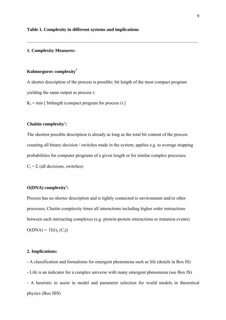
Table 1. Complexity in different systems and implications

___________________________________________________________________________

1. Complexity Measures:

Kolmorgorov complexity*

A shorter description of the process is possible; bit length of the most compact program

yielding the same output as process i:

Ki = min [ bitlength (compact program for process i) ]

Chaitin complexity†:

The shortest possible description is already as long as the total bit content of the process

counting all binary decision / switches made in the system; applies e.g. to average stopping

probabilities for computer programs of a given length or for similar complex processes.

Ci = Σ (all decisions, switches)

O(DNA) complexity‡:

Process has no shorter description and is tightly connected to environment and/or other

processes; Chaitin complexity times all interactions including higher order interactions

between such interacting complexes (e.g. protein-protein interactions or mutation events)

O(DNA) = Π(Πij (Ci))

2. Implications:

- A classification and formalisms for emergent phenomena such as life (details in Box IS)

- Life is an indicator for a complex universe with many emergent phenomena (see Box IS)

- A heuristic to assist in model and parameter selection for world models in theoretical

physics (Box IIIS)

10

___________________________________________________________________________

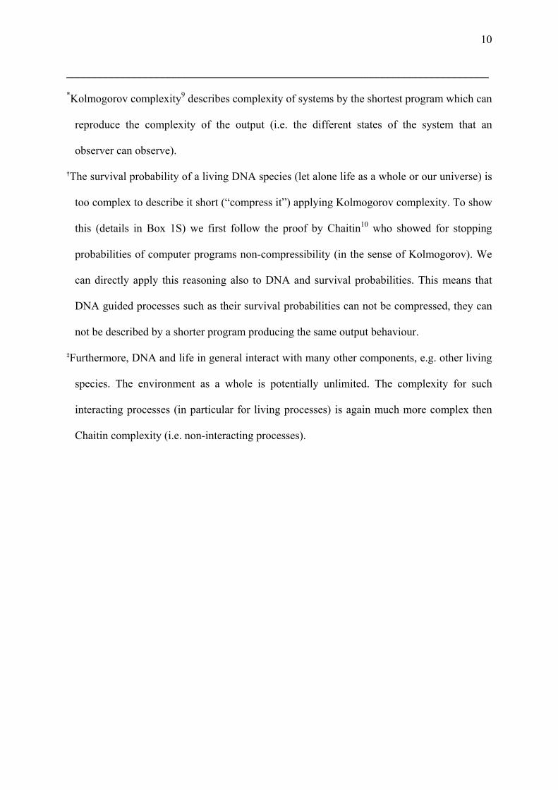
*Kolmogorov complexity9 describes complexity of systems by the shortest program which can

reproduce the complexity of the output (i.e. the different states of the system that an

observer can observe).

†The survival probability of a living DNA species (let alone life as a whole or our universe) is

too complex to describe it short (“compress it”) applying Kolmogorov complexity. To show

this (details in Box 1S) we first follow the proof by Chaitin10 who showed for stopping

probabilities of computer programs non-compressibility (in the sense of Kolmogorov). We

can directly apply this reasoning also to DNA and survival probabilities. This means that

DNA guided processes such as their survival probabilities can not be compressed, they can

not be described by a shorter program producing the same output behaviour.

‡Furthermore, DNA and life in general interact with many other components, e.g. other living

species. The environment as a whole is potentially unlimited. The complexity for such

interacting processes (in particular for living processes) is again much more complex then

Chaitin complexity (i.e. non-interacting processes).

11

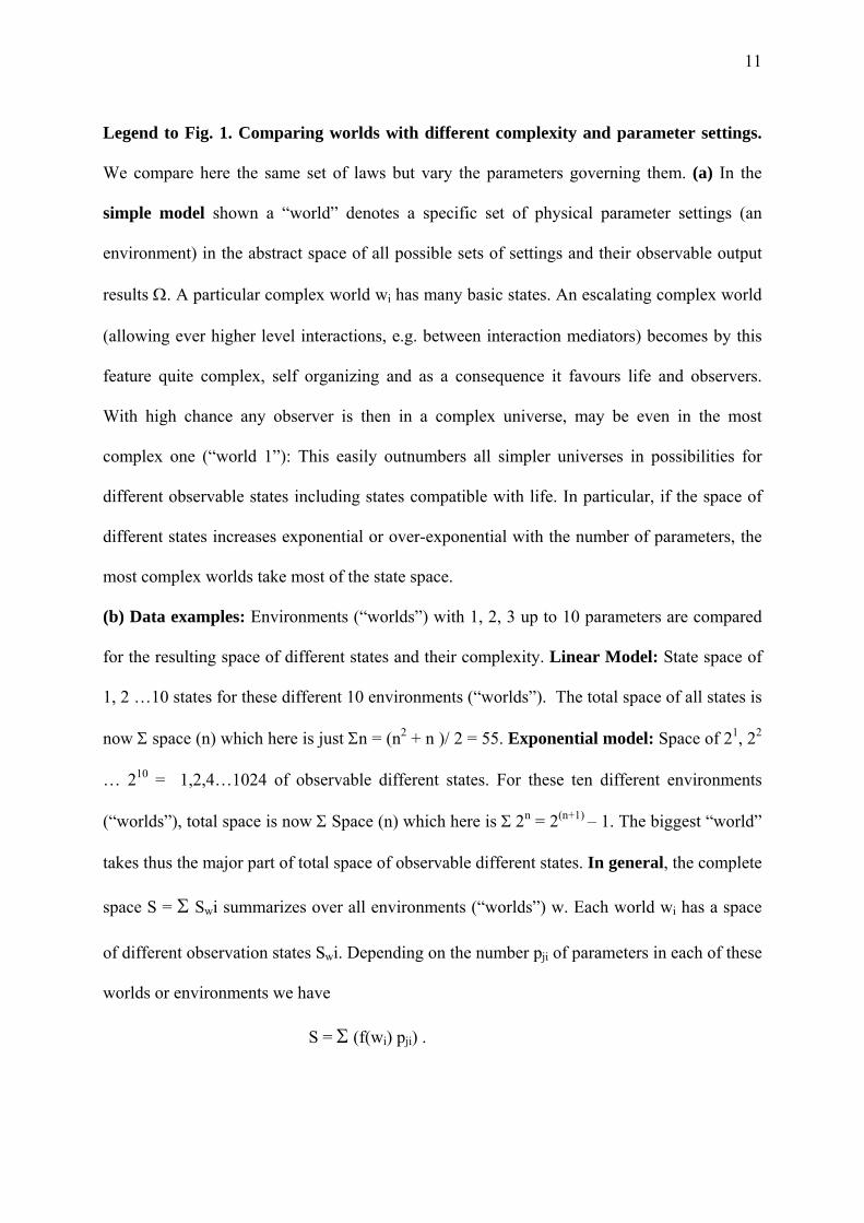
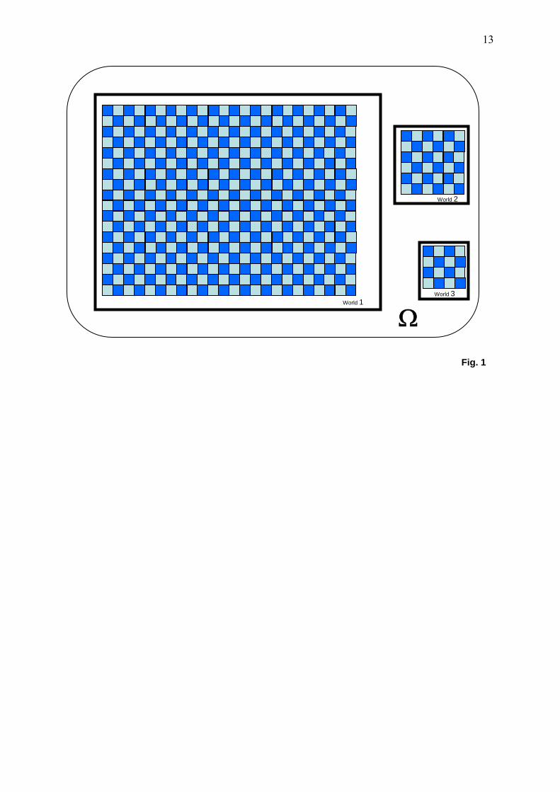
Legend to Fig. 1. Comparing worlds with different complexity and parameter settings.

We compare here the same set of laws but vary the parameters governing them. (a) In the

simple model shown a “world” denotes a specific set of physical parameter settings (an

environment) in the abstract space of all possible sets of settings and their observable output

results Ω. A particular complex world wi has many basic states. An escalating complex world

(allowing ever higher level interactions, e.g. between interaction mediators) becomes by this

feature quite complex, self organizing and as a consequence it favours life and observers.

With high chance any observer is then in a complex universe, may be even in the most

complex one (“world 1”): This easily outnumbers all simpler universes in possibilities for

different observable states including states compatible with life. In particular, if the space of

different states increases exponential or over-exponential with the number of parameters, the

most complex worlds take most of the state space.

(b) Data examples: Environments (“worlds”) with 1, 2, 3 up to 10 parameters are compared

for the resulting space of different states and their complexity. Linear Model: State space of

1, 2 …10 states for these different 10 environments (“worlds”). The total space of all states is

now Σ space (n) which here is just Σn = (n2 + n )/ 2 = 55. Exponential model: Space of 21, 22

… 210 = 1,2,4…1024 of observable different states. For these ten different environments

(“worlds”), total space is now Σ Space (n) which here is Σ 2n = 2(n+1) – 1. The biggest “world”

takes thus the major part of total space of observable different states. In general, the complete

space S = Σ Swi summarizes over all environments (“worlds”) w. Each world wi has a space

of different observation states Swi. Depending on the number pji of parameters in each of these

worlds or environments we have

S = Σ (f(wi) pji) .

12

Already for moderate non-linear functions f(wi) (e.g. exponential) the parameter-rich worlds

(or, more moderate, the environments which favour stable conditions and complexity) take

major slices of the total space.

(c) Detailed comparison and calculation: We give as an example calculations based on

discrete histories in quantum spin-loop theory (Box IIS)

Methods: Mathematical analysis; test calculations where done on a standard PC; formalisms,

detailed calculations and complexity comparisons are given in suppl. Material.

13

Ω World 3

World 2

World 1

Fig. 1

14

Supplementary Material (Summary; Table 1S; Box IS, IIS and IIIS)

Why are nature´s constants so fine-tuned? The case for an escalating complex universe

Thomas Dandekar1,2

1Department of Bioinformatics, University of Würzburg, Biozentrum, Am Hubland D-97074 Würzburg; and 2EMBL, Postfach 102209, D-69012 Heidelberg, Germany Contact: dandekar@biozentrum.uni-wuerzburg.de Tel. +49-(0)931-888-4551 Fax. +49-(0)931-8884552

Summary Figure: Flow diagram of the results

Multiverse Paradox: A multiverse implies myriads of possibilities where a universe with life is a very rare accident. However, the Copernican principle suggests on the contrary, our observation point should not be special or extremely rare

Our solution: Complex worlds have a very large space of different states and take a major fraction of the total of all possible states and that is the reason why a world allowing an observer is far more probable then one without. Simple test: model calculations (Fig. 1).

Anthropocentric principle can be reinterpreted: The complexity of observable different states if there would be alternative parameter settings for physical laws will be less for less complex worlds (e.g. without an observer) (Table 1S).

Formalize different levels of complexity (Table 1); complex output behaviour is sufficient to cover complex processes such as dynamic systems and life. However, this requires complex output behaviour that no longer can be simplified by a shorter (Kolmogorov) description. This has applications and implications for life and self organizing processes (Box IS, text).

The world complexity (Fig. 1) for different parameter settings (Table 1S) can be directly calculated. Example: discrete histories from quantum spin-loop theory (Box IIS).

The observation that our world is highly complex (Table 1, Box IS) can be used as a heuristic to decide which parameter setting to choose in fundamental theories of physics (Box IIIS).

15

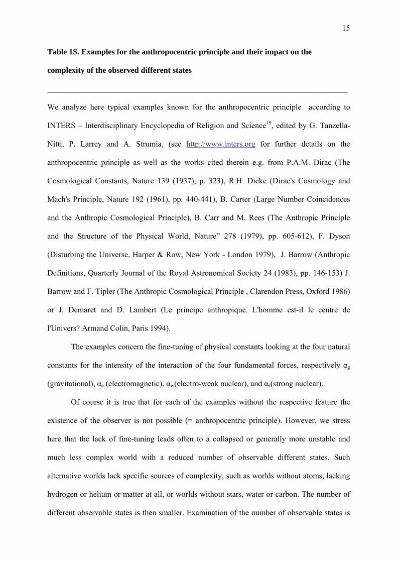
Table 1S. Examples for the anthropocentric principle and their impact on the

complexity of the observed different states

___________________________________________________________________________

We analyze here typical examples known for the anthropocentric principle according to

INTERS – Interdisciplinary Encyclopedia of Religion and Science19, edited by G. Tanzella-

Nitti, P. Larrey and A. Strumia, (see http://www.inters.org for further details on the

anthropocentric principle as well as the works cited therein e.g. from P.A.M. Dirac (The

Cosmological Constants, Nature 139 (1937), p. 323), R.H. Dicke (Dirac's Cosmology and

Mach's Principle, Nature 192 (1961), pp. 440-441), B. Carter (Large Number Coincidences

and the Anthropic Cosmological Principle), B. Carr and M. Rees (The Anthropic Principle

and the Structure of the Physical World, Nature” 278 (1979), pp. 605-612), F. Dyson

(Disturbing the Universe, Harper & Row, New York - London 1979), J. Barrow (Anthropic

Definitions, Quarterly Journal of the Royal Astronomical Society 24 (1983), pp. 146-153) J.

Barrow and F. Tipler (The Anthropic Cosmological Principle , Clarendon Press, Oxford 1986)

or J. Demaret and D. Lambert (Le principe anthropique. L'homme est-il le centre de

l'Univers? Armand Colin, Paris 1994).

The examples concern the fine-tuning of physical constants looking at the four natural

constants for the intensity of the interaction of the four fundamental forces, respectively αg

(gravitational), αe (electromagnetic), αw(electro-weak nuclear), and αs(strong nuclear).

Of course it is true that for each of the examples without the respective feature the

existence of the observer is not possible (= anthropocentric principle). However, we stress

here that the lack of fine-tuning leads often to a collapsed or generally more unstable and

much less complex world with a reduced number of observable different states. Such

alternative worlds lack specific sources of complexity, such as worlds without atoms, lacking

hydrogen or helium or matter at all, or worlds without stars, water or carbon. The number of

different observable states is then smaller. Examination of the number of observable states is

16

explanatory for many phenomena of fine-tuning, in particular such that allow better stability

or, for instance, additional reactions (see examples). The argument is also directly testable by

the examples: Many conditions listed here improve stability for complex states and

complexity as well as the richness of different observable states, but have not directly to do

with our anthropocentric, specific existence (see also the list of phenomena where there is

over-tuning, e.g. regarding the stability of the proton).

Examples:

- αg the gravitational force, determines the initial rate of expansion of the universe: a

higher value then that actually observed leads to a collapse of the whole universe on itself

(more or less immediately after its start); however, if the value would be a little bit lower,

there would have been no gravitational aggregation of matter, implying no formation of

galaxies, stars or planets and low complexity of the resulting universe.

- About 1 sec after the Big Bang, neutrinos are decoupled from the rest of the

matter, this conserves the ratio between the number of protons and neutrons. The ratio

depends very sensitively upon the expansion rate i.e. αg and on the intensity of the weak

interaction αw regarding the decay of the neutron. However, formation of helium directly from

the Big Bang depends on the ratio of protons to neutrons and, thus, upon the ratio αg/αw. If this

ratio is slightly higher, all protons would be transformed into nuclei of helium, there would be

no hydrogen and, in consequence, no water. In contrast, a lower value looses the abundance of

cosmological helium, with negative impact on the thermodynamic evolution of stars

(extremely rapid star evolution, in general much too unstable and short for life to evolve on

planets).

- The ratio a αs/αe is critical for chemistry. The strong nuclear force has to be

strong in interactions at a very short range to allow stable atomic nuclei; otherwise there

would be no periodic table of chemical elements. If αe would be a little bit larger, or αs would

be a bit smaller, even the lightest nuclei would not have been stable. Of course also the exact

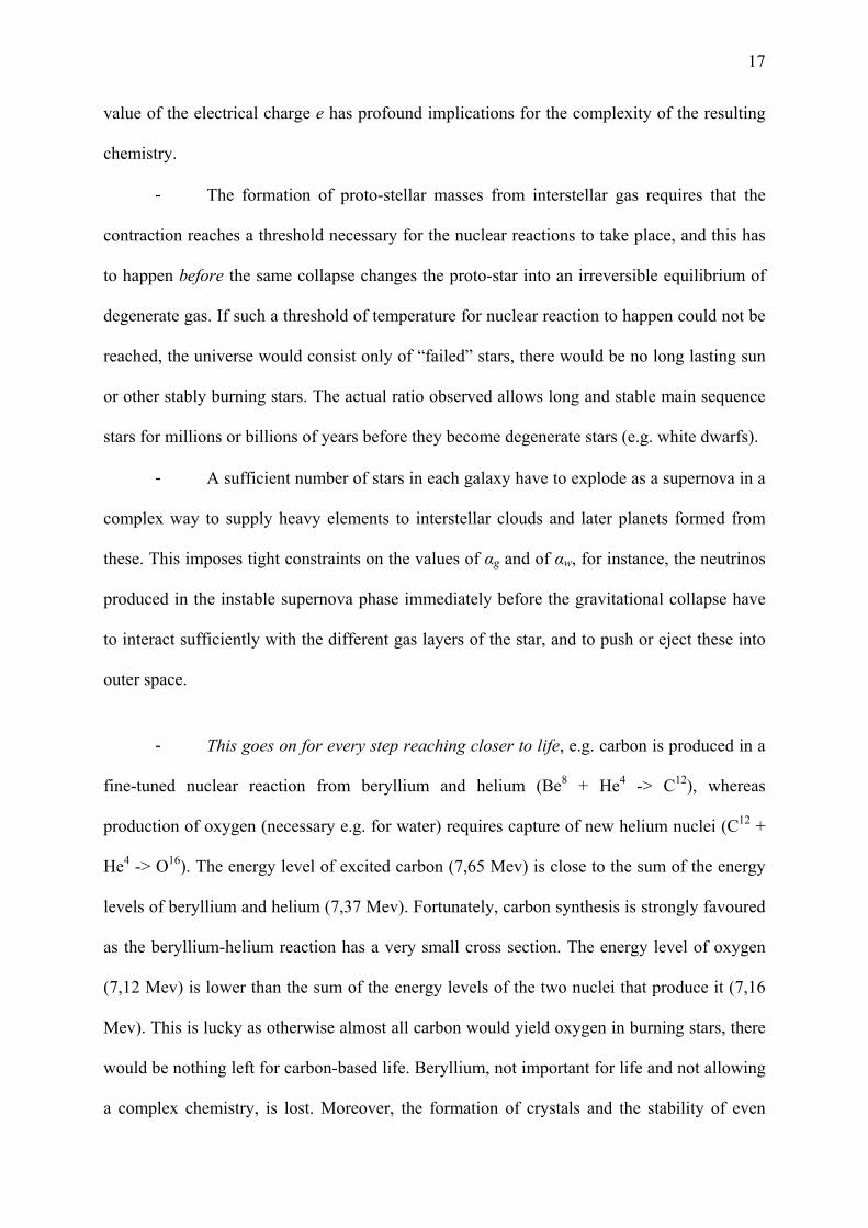
17

value of the electrical charge e has profound implications for the complexity of the resulting

chemistry.

- The formation of proto-stellar masses from interstellar gas requires that the

contraction reaches a threshold necessary for the nuclear reactions to take place, and this has

to happen before the same collapse changes the proto-star into an irreversible equilibrium of

degenerate gas. If such a threshold of temperature for nuclear reaction to happen could not be

reached, the universe would consist only of “failed” stars, there would be no long lasting sun

or other stably burning stars. The actual ratio observed allows long and stable main sequence

stars for millions or billions of years before they become degenerate stars (e.g. white dwarfs).

- A sufficient number of stars in each galaxy have to explode as a supernova in a

complex way to supply heavy elements to interstellar clouds and later planets formed from

these. This imposes tight constraints on the values of αg and of αw, for instance, the neutrinos

produced in the instable supernova phase immediately before the gravitational collapse have

to interact sufficiently with the different gas layers of the star, and to push or eject these into

outer space.

- This goes on for every step reaching closer to life, e.g. carbon is produced in a

fine-tuned nuclear reaction from beryllium and helium (Be8 + He4 -> C12), whereas

production of oxygen (necessary e.g. for water) requires capture of new helium nuclei (C12 +

He4 -> O16). The energy level of excited carbon (7,65 Mev) is close to the sum of the energy

levels of beryllium and helium (7,37 Mev). Fortunately, carbon synthesis is strongly favoured

as the beryllium-helium reaction has a very small cross section. The energy level of oxygen

(7,12 Mev) is lower than the sum of the energy levels of the two nuclei that produce it (7,16

Mev). This is lucky as otherwise almost all carbon would yield oxygen in burning stars, there

would be nothing left for carbon-based life. Beryllium, not important for life and not allowing

a complex chemistry, is lost. Moreover, the formation of crystals and the stability of even

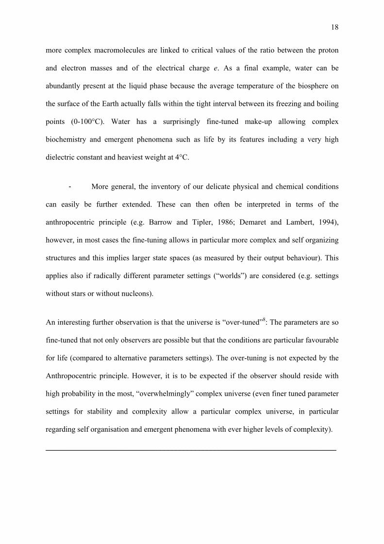
18

more complex macromolecules are linked to critical values of the ratio between the proton

and electron masses and of the electrical charge e. As a final example, water can be

abundantly present at the liquid phase because the average temperature of the biosphere on

the surface of the Earth actually falls within the tight interval between its freezing and boiling

points (0-100°C). Water has a surprisingly fine-tuned make-up allowing complex

biochemistry and emergent phenomena such as life by its features including a very high

dielectric constant and heaviest weight at 4°C.

- More general, the inventory of our delicate physical and chemical conditions

can easily be further extended. These can then often be interpreted in terms of the

anthropocentric principle (e.g. Barrow and Tipler, 1986; Demaret and Lambert, 1994),

however, in most cases the fine-tuning allows in particular more complex and self organizing

structures and this implies larger state spaces (as measured by their output behaviour). This

applies also if radically different parameter settings (“worlds”) are considered (e.g. settings

without stars or without nucleons).

An interesting further observation is that the universe is “over-tuned”8: The parameters are so

fine-tuned that not only observers are possible but that the conditions are particular favourable

for life (compared to alternative parameters settings). The over-tuning is not expected by the

Anthropocentric principle. However, it is to be expected if the observer should reside with

high probability in the most, “overwhelmingly” complex universe (even finer tuned parameter

settings for stability and complexity allow a particular complex universe, in particular

regarding self organisation and emergent phenomena with ever higher levels of complexity).

___________________________________________________________________________

19

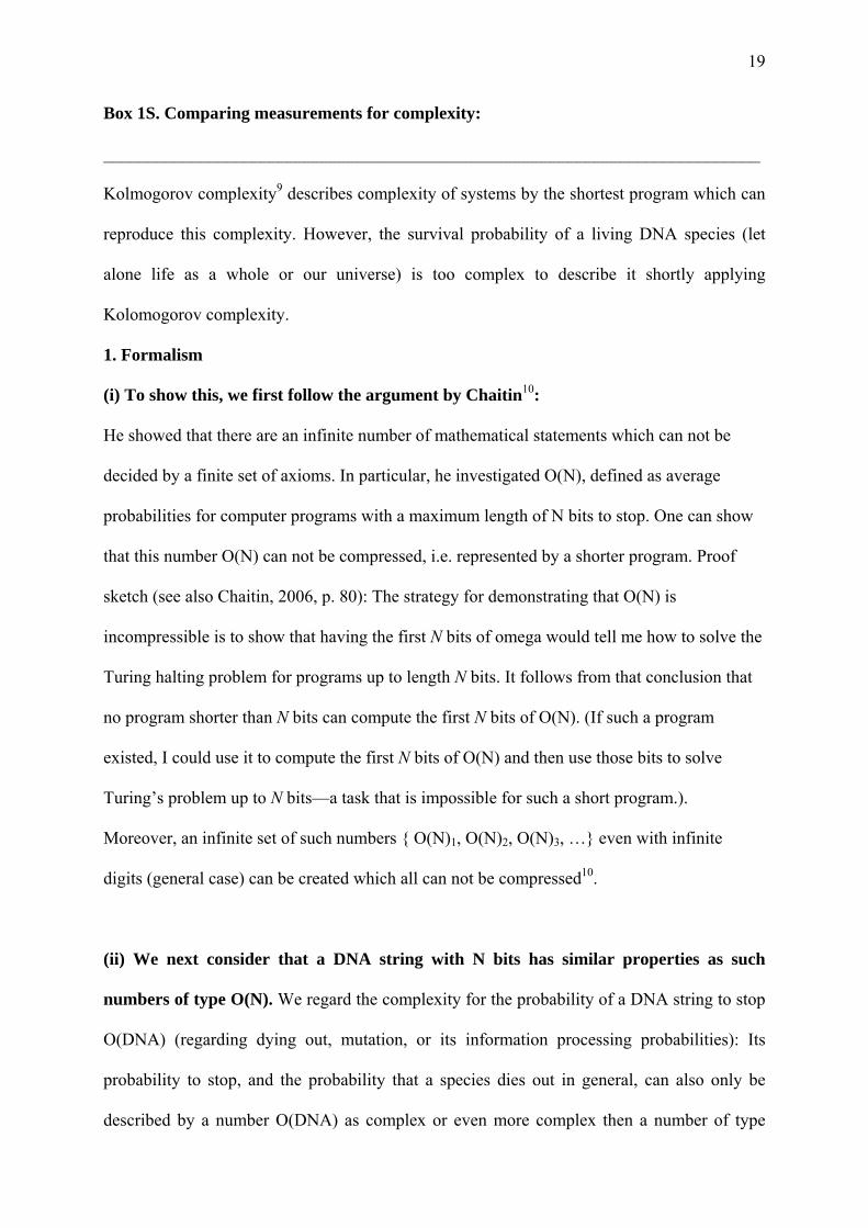
Box 1S. Comparing measurements for complexity:

___________________________________________________________________________

Kolmogorov complexity9 describes complexity of systems by the shortest program which can

reproduce this complexity. However, the survival probability of a living DNA species (let

alone life as a whole or our universe) is too complex to describe it shortly applying

Kolomogorov complexity.

1. Formalism

(i) To show this, we first follow the argument by Chaitin10:

He showed that there are an infinite number of mathematical statements which can not be

decided by a finite set of axioms. In particular, he investigated O(N), defined as average

probabilities for computer programs with a maximum length of N bits to stop. One can show

that this number O(N) can not be compressed, i.e. represented by a shorter program. Proof

sketch (see also Chaitin, 2006, p. 80): The strategy for demonstrating that O(N) is

incompressible is to show that having the first N bits of omega would tell me how to solve the

Turing halting problem for programs up to length N bits. It follows from that conclusion that

no program shorter than N bits can compute the first N bits of O(N). (If such a program

existed, I could use it to compute the first N bits of O(N) and then use those bits to solve

Turing’s problem up to N bits—a task that is impossible for such a short program.).

Moreover, an infinite set of such numbers { O(N)1, O(N)2, O(N)3, …} even with infinite

digits (general case) can be created which all can not be compressed10.

(ii) We next consider that a DNA string with N bits has similar properties as such

numbers of type O(N). We regard the complexity for the probability of a DNA string to stop

O(DNA) (regarding dying out, mutation, or its information processing probabilities): Its

probability to stop, and the probability that a species dies out in general, can also only be

described by a number O(DNA) as complex or even more complex then a number of type

20

O(N). There are several reasons for this, one is that the halting problem for any DNA based

organism replicating with copy number r and probability p(r) is more then Turing complex

and NP complete14. Furthermore, consider that the probabilities for mutation are in a

potentially infinite context (e.g. probabilities of mutation p(m) depend among other things

from ionizing radiation which may come from very distant stars or even quasars) and that

both mutations and survival are stochastic processes. Both add sufficient to the halting

problem regarding a DNA and a species (a population of DNAs, DNAvectori ) that its average

stopping probabilities (or survival, mutation, information processing probabilities etc.) only

can be properly described by non compressible numbers O(N)DNA at least as complex as

O(N):

O(N)DNA=O(DNAvectori x(r x p(r))x(1-p(m))x(1-p(Π(selection at all levelsii in enviromentsij)))) ii,ij

However, O(N) numbers measure complexity resulting from averages over discrete, closed

programs (or processes) which each are independent. In contrast, O(N)DNA numbers consider

averages over open processes, interacting with an open (potentially unlimited) environment.

(iii) We cast this into a formalism describing the complexity of an object or even a

world. The number of all contained Kolmogorov processes Κ is compactly described by a

program C(Κ) with length l, and we collect all non-compressible phenomena from the type of

O(N) numbers (process averages, stopping probabilities etc.) as well as all more complex

interacting non-compressible phenomena such as life (O(DNA) numbers e.g. species, DNAs,

other self organizing and selfermergent processes)

Complexity (object) = length (C(Κ)) + { O(N)1, O(N)2, …} + { O(DNA)1, O(DNA)2, …}

21

This implies comparing very high up to infinite sets of non-compressible numbers if we want

to compare the complexity of objects and in particular the complexity of different worlds

(with their variations in their laws of physics). However, this can be done with set theory even

for infinite sets and their cardinality. This furthermore shows that our world has no simple

description, e.g. in contrast to 15.

2. Consequences: To get such large state spaces, both information storage and processing of

this stored information (catalysis) is necessary. Note that “bits” in this sense is non-trivial and

only possible in a rather complex universe (difference to simpler definitions for bits who just

consider two states for quanta or particles): “Bits” implies here already an observer or a

(molecular) program to be properly processed. Furthermore, living processes evolve

(including their stored information) to ever higher levels (genetic level: evolution; next higher

level: learning, understanding / meaning16; next higher level: culture). These properties

(catalysis, information storage) are necessary consequences if the parameter set of the

physical laws with a maximum size of different observable states is taken. This is also true for

self organization with emergent ever higher levels of interactions (potentially unlimited and

reaching out to very far distances, e.g. mutations include hits from radiation of very distant

stars or quasars) as well as ever new types of interactions (from DNA to neurons, then

language, next computer programs, internet and so on). In fact, this can be developed to a

complete theory (not shown here) of life and adaptation comparing cellular life in terms of

objective different states including general metabolic state space17, regulatory implications18

and a new “background free” (as in quantum spin-loop theory16) description of evolution.

3. Applications: To exist in an escalating complex universe is sufficient to have phenomena

such as life as well as many other phenomena of self organization and ongoing evolution to

ever higher levels of complexity. Note that elementary states (nodes) and interactions between

22

them (edges) can quickly become rather complex even with a comparatively limited number

of elementary states if the escalating property holds and interactions of interactions (as super-

nodes) are iteratively possible. As with recursive functions in general (e.g. Ackermann

function) such a space of different states becomes quickly very large. One further level of

recursion more leads to an excessive larger space of different states; hence the most complex

world probably owns the largest slice of the complete space (Fig. 1).

Self organizing phenomena can be classified and described according to the four levels of

complexity given ((i) Kolmogorov; (ii) Chaitin; (iii) DNA-like including interacting processes

and (iv) iterative emergent. For instance, DNA-based life can be classified in this way

regarding replication (Cell cycle, regulation, number of complexity generating cycles) or

regarding growth (including metabolism and its regulation).

Tools to classify and understand complex processes including life can be understood and

further developed applying these four classes and measures of complexity. The number of

different states is again central. Biological application examples include

(i) analysis and approaches for the calculation of the number of different metabolic

states or pathways, for instance applying elementary mode analysis17.

(ii) The analysis of regulatory networks, in particular the number of stable system

states requires negative feed-back loops whereas the number of different system

states increases exponentially with the number of positive feedback loops (e.g.22).

The size of different states correlates also directly with network size, for instance

in interactome studies of the proteome, different subnetworks depend on the

balance between kinases and phosphatases23, furthermore different modules shape

building blocks of 3- and 4-protein complexes and this modular structure again

leads to high adaptability and a high number of system states, for instance in the

adhesome24. Regarding complexity and emergent phenomena, the coupling of the

different processes is critical (see Table 1; differences between Chaitin complexity

23

and O(DNA) complexity or processes). Thus an analysis of how the size of

different states increases with tighter coupling can directly be applied in

neurobiology to compare different processing units and their processing

capabilities as well as their emergent potential (not shown here).

24

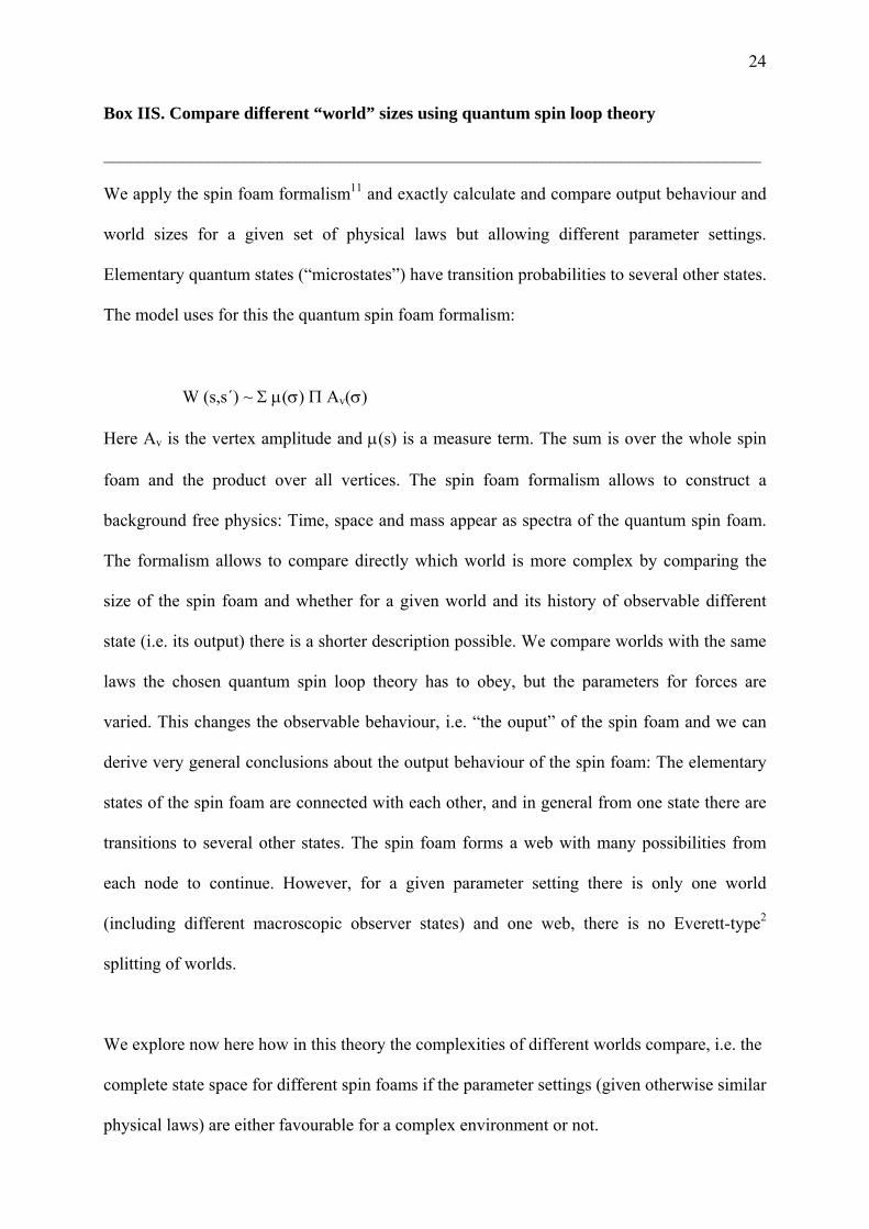
Box IIS. Compare different “world” sizes using quantum spin loop theory

___________________________________________________________________________

We apply the spin foam formalism11 and exactly calculate and compare output behaviour and

world sizes for a given set of physical laws but allowing different parameter settings.

Elementary quantum states (“microstates”) have transition probabilities to several other states.

The model uses for this the quantum spin foam formalism:

W (s,s´) ~ Σ μ(σ) Π Av(σ) Here Av is the vertex amplitude and μ(s) is a measure term. The sum is over the whole spin

foam and the product over all vertices. The spin foam formalism allows to construct a

background free physics: Time, space and mass appear as spectra of the quantum spin foam.

The formalism allows to compare directly which world is more complex by comparing the

size of the spin foam and whether for a given world and its history of observable different

state (i.e. its output) there is a shorter description possible. We compare worlds with the same

laws the chosen quantum spin loop theory has to obey, but the parameters for forces are

varied. This changes the observable behaviour, i.e. “the ouput” of the spin foam and we can

derive very general conclusions about the output behaviour of the spin foam: The elementary

states of the spin foam are connected with each other, and in general from one state there are

transitions to several other states. The spin foam forms a web with many possibilities from

each node to continue. However, for a given parameter setting there is only one world

(including different macroscopic observer states) and one web, there is no Everett-type2

splitting of worlds.

We explore now here how in this theory the complexities of different worlds compare, i.e. the

complete state space for different spin foams if the parameter settings (given otherwise similar

physical laws) are either favourable for a complex environment or not.

25

Consider a nonrelativistic one-dimensional quantum system with x as its dynamic variable.

The propagator W(x,t,x´,t´) then contains the full dynamic information about the system.

According to Feynman the propagator can be expressed as a path integral

W(x,t,x´,t´) ~ ∫ D[x(t)]eiS[x] in which the sum is over the paths x(t) that start at (x´,t´) and end at (x,t) and S[x] is the action

of this paths. This basic definition of the quantum formalism can then be used to calculate

sums of complex amplitudes eiS[x] over the paths x(t).

In particular, the functional integral is then defined as:

[ ]

'|| ||

|| ||

)(

)'(H

11

)'(H

2

2

)'(H

11

)'(H

11

')'()(

][

00

00

lim

xexxex

xexxex

dxdxetxD

Ntti

Ntti

NN

tti

NNNtti

N

xtxxtx N

xiS

−−

−−

−

−−

−−

−−

−

== ∞→

∫∫ ≡

K

K

Similarly, one can of course also use sum-over-paths formalisms for quantum gravity and

would then derive path integrals over 4d metrics. However, following Rovelli16 (pp. 320ff), in

the background-free quantum spin loop formalism this corresponds to a discrete sum over

histories of spin networks. Transition probabilities are between spin networks. The quantity x

in the argument of the propagator is not the classical variable but rather a label of an

eigenstate of this variable. The transition amplitude is not expressed as an integral over 4d

fields but rather as a discrete sum-over-histories s of spin networks. This yields a spin foam:

W(s,s´) = Σ A(σ) σ

A history is a discrete sequence σ = (s, sN,…,s1,s´) of spin networks. In particular, in this

background free scenario, this corresponds to count nodes and ages of the spin foam and

compare different sizes of spin foams.

26

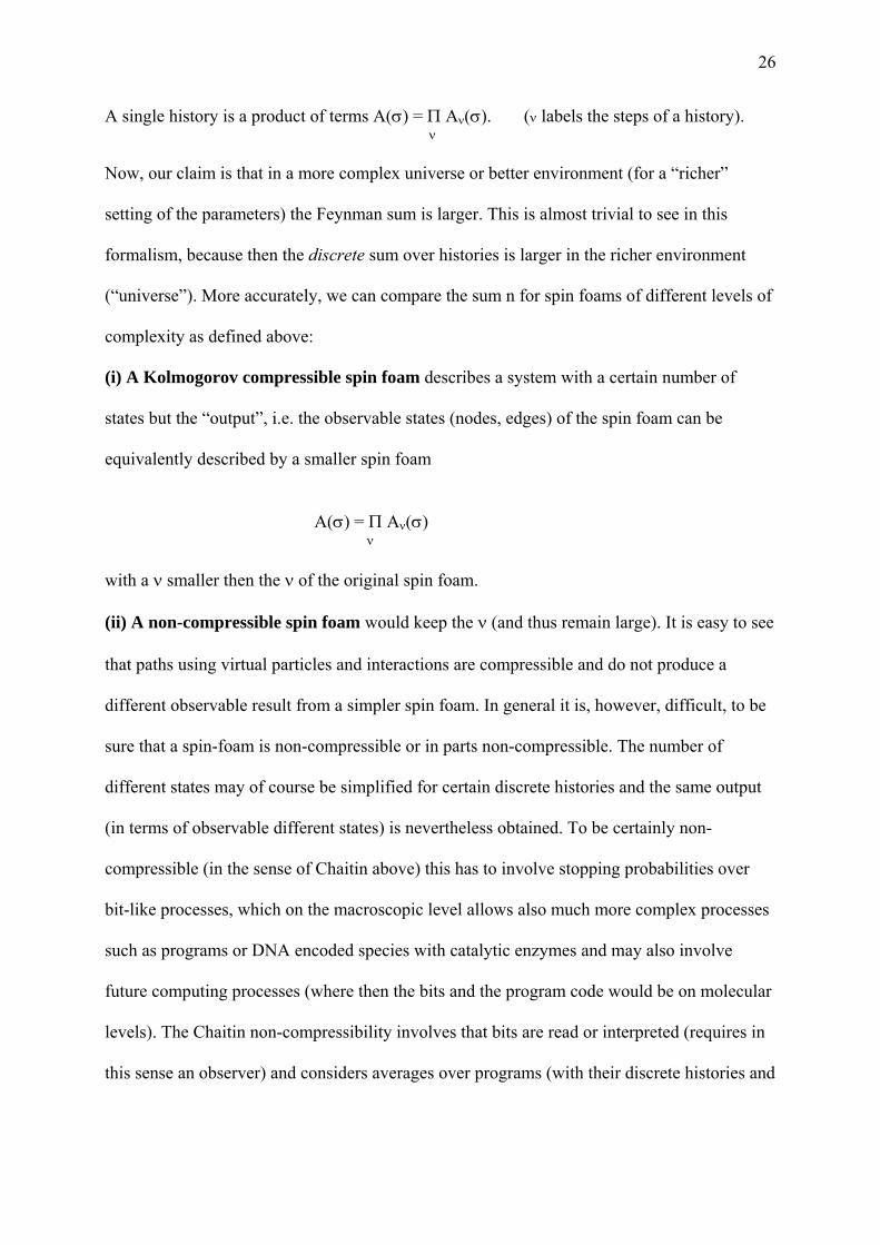
A single history is a product of terms A(σ) = Π Aν(σ). (ν labels the steps of a history). ν Now, our claim is that in a more complex universe or better environment (for a “richer”

setting of the parameters) the Feynman sum is larger. This is almost trivial to see in this

formalism, because then the discrete sum over histories is larger in the richer environment

(“universe”). More accurately, we can compare the sum n for spin foams of different levels of

complexity as defined above:

(i) A Kolmogorov compressible spin foam describes a system with a certain number of

states but the “output”, i.e. the observable states (nodes, edges) of the spin foam can be

equivalently described by a smaller spin foam

A(σ) = Π Aν(σ)

ν with a ν smaller then the ν of the original spin foam. (ii) A non-compressible spin foam would keep the ν (and thus remain large). It is easy to see

that paths using virtual particles and interactions are compressible and do not produce a

different observable result from a simpler spin foam. In general it is, however, difficult, to be

sure that a spin-foam is non-compressible or in parts non-compressible. The number of

different states may of course be simplified for certain discrete histories and the same output

(in terms of observable different states) is nevertheless obtained. To be certainly non-

compressible (in the sense of Chaitin above) this has to involve stopping probabilities over

bit-like processes, which on the macroscopic level allows also much more complex processes

such as programs or DNA encoded species with catalytic enzymes and may also involve

future computing processes (where then the bits and the program code would be on molecular

levels). The Chaitin non-compressibility involves that bits are read or interpreted (requires in

this sense an observer) and considers averages over programs (with their discrete histories and

27

output). Only this makes the strong statement possible that such a spin foam can in this aspect

certainly not be simplified.

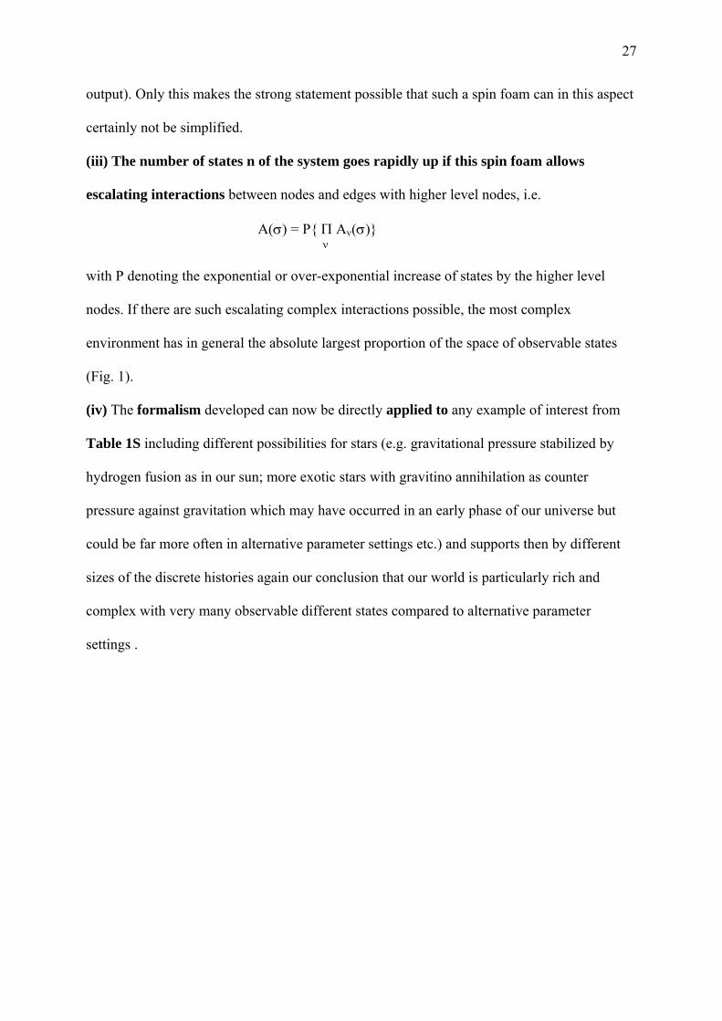
(iii) The number of states n of the system goes rapidly up if this spin foam allows

escalating interactions between nodes and edges with higher level nodes, i.e.

A(σ) = P{ Π Aν(σ)} ν with P denoting the exponential or over-exponential increase of states by the higher level

nodes. If there are such escalating complex interactions possible, the most complex

environment has in general the absolute largest proportion of the space of observable states

(Fig. 1).

(iv) The formalism developed can now be directly applied to any example of interest from

Table 1S including different possibilities for stars (e.g. gravitational pressure stabilized by

hydrogen fusion as in our sun; more exotic stars with gravitino annihilation as counter

pressure against gravitation which may have occurred in an early phase of our universe but

could be far more often in alternative parameter settings etc.) and supports then by different

sizes of the discrete histories again our conclusion that our world is particularly rich and

complex with very many observable different states compared to alternative parameter

settings .

28

Box IIIS. Applying our argument to unified theories.

___________________________________________________________________________ Unified theories strive for a unification of all four basic forces. To discuss here all efforts

towards the direction of such a “theory of everything” (TOE) is beyond the limits of this

article. Instead we will point out here how the principle that an observer tends to reside in a

typical observation point (Copernican principle4) and, hence, with high probability in a

universe with very many different states can also here identify best choices of parameters.

Basic symmetries.

String theory represents all 4 basic forces and particle families by geometric symmetries in a

high dimensional space (10 for the five well known string theories or 11 for the unifying M-

theory. The additional dimensions are compactified to yield our normal world with time and

space (four dimensions) and, to be realistic, with a flat Ricci Metric20. However, interestingly,

as the five well known string theories are related to each other and again for the reason of the

basic symmetry and particle requirements of the basic four forces, these string theories rely on

the E8 group (as does for instance the exceptionally simple TOE by Lisi21 [which probably is

too simple, at least regarding Lie algebras]). The reliance on the E8 group is most clearly seen

in the heterotic string theory. Here the transition from 26 dimensions to 4 dimensions occurs

in two steps. First 16 of the original 26 dimensions compactify in a self-consistent way; then 6

of the remaining 10 dimensions. The E8 symmetry arises in heterotic string theory from the

reduction from 26 to 10 dimensions. One needs to endow a 16-dimensional subspace of the

orginal 26-dimensional space with an even, unimodular lattice. There are exactly two such

lattices in 16 dimensions, one of which is the root lattice of E8+E8. Moreover, in Heterotic

string theory the first E8 symmetry can elegantly be used to describe the richness of all our

observed particles and interactions of our every day physics (the “four basic forces”), whereas

29

the second E8 symmetry allows to derive predictions for missing particles and interactions,

e.g. regarding dark matter.

The E8 group is the exceptional Lie group E8. An atlas of Lie groups and representations was

achieved recently (http://www.aimath.org/E8/). The magnitude of the E8 calculation is

enormous, 60 gigabytes in size (the human genome is less than a gigabyte in size). The

accumulated data on E8 will need long time of analysis and could have unforeseen

implications in mathematics and physics.

However, in complete support of our claim, E8 is first of all the largest exceptional or

in other words the most complex finite root system ( as a set of vectors in an 8-dimensional

real vector space satisfying certain properties). If an observer exists in a universe, he should

with highest probability reside in the universe which has most complexity and that applies for

finite root systems to E8.

Root systems were classified by Wilhelm Killing in the 1890s. He found four infinite classes

of Lie algebras, and labelled them An, Bn, Cn, and Dn, where n=1,2,3.... He also found five

exceptional ones: G2, F4, E6, E7, and E8. According to our claim, the most complex possibility

allows the largest state space of different configurations or states and this is for finite Lie

algebras the E8 symmetrie group. Infinite Lie algebras have many reasons why they are not

compatible with our observed physics (in particular, it becomes difficult then to identify

particle families or other observable features).

String theory parameter setting. There are many ways to achieve a String theory, in

particular theories with 5 scaling variables to comprise the complete class of 7555

quasismooth Calabi-Yau hypersurfaces embedded in weighted 4-space. Furthermore, there are

3,284 theories with more than five variables deining higher-dimensioal manifolds, so called

Special Fano Varieties or generalized Calabi-Yau manifolds . The topological holes in the

30

manifold or in other words the string spectra have to fit our observed particles (number,

properties, charges) to be realistic. A way to compare such complexities is the counting of

instantons. This is an incomplete description of state space as only these are counted, but

would give a first estimate. A Mathematica program to calculate this is available from

http://www.th.physik.uni-bonn.de/th/People/netah/cy/codes/inst.m

String theory is a very elegant and powerful theoretical framework. Nevertheless, currently

there are too many free parameters and in that sense it is currently a “non falsifiable theory “

which is always correct as one of the many possibilities could still fit all observed data.

Furthermore, all these possibilities are also difficult to calculate in detail to derive the

observed spectrum of particles and often postulate many more particles not [yet] observed.

If string theory turns out to be correct (either based on Calabi-Yau manifolds or alternative

versions, e.g. based on G2 holonomy manifolds) or becomes part of an even more complete

theory our claim would be that the solution with the most complex space of different states is

that one which we have also the highest probability to reside in, and hence, most probable will

yield the correct string spectrum to fit with our observed particles.

The major implication is that measuring the complexity and the output state number (output

size) of the different string theory versions is an objective criterion to allow a rational and

correct choice of the correct string theory instead of an arbitrary choice (or in fact, an

undecided plethora of possibilities).

31

Additional References Supp. Material:

14. Csuhaj-Varju E, Freund R, Kari L, Paun G. DNA computing based on splicing:

universality results, pp. 179-190 in Pac Symp Biocomput. 1996; Ed. by L. Hunter and

T. E. Klein. World Scientific Publishing Co., Singapore, 1996..

15. Wolfram, Stephen “A New Kind of Science” Wolfram Media Inc. Champaign Illinois

(2002).

16. Figge, Udo L. Jakob von Uexküll: Merkmale and Wirkmale. Semiotica 134, 193-200

(2001).

17. Schuster S, Fell DA, Dandekar T. A general definition of metabolic pathways useful for

systematic organization and analysis of complex metabolic networks. Nature

Biotechnol. 18, 326-32 (2000).

18. Robubi, A., Mueller. T., Fueller,J., Hekman,M., Rapp,U.R. und Dandekar, T.

B-Raf and C-Raf signaling investigated in a simplified model of the mitogenic kinase

cascade. Biol. Chemistry 386, 1165-1171 und Sup36-Sup37 (2005).

19. INTERS – Interdisciplinary Encyclopedia of Religion and Science, edited by G. Tanzella-

Nitti, P. Larrey and A. Strumia, see http://www.inters.org

20. Gross, M., Huybrechts, D., Joyce,D. Calabi-Yau Manifolds and Related Geomeries.

Springer, New York, 2003. ISBN 354-04-4059-3

21. Lisi, A.G. An exceptionally simple theory of everything. (6 Nov 2007, preprint on

arXiv:0711.0770 preprint server)

22. Skotheim, J.M., Di Talia, S., Siggia, E.D, Cross, F.R. Positive feedback of G1 cyclins

ensures coherent cell cycle entry. Nature 454, 291-296 (2008).

23. Dittrich,M., Birschmann,I., Mietner,S., Sickmann, A., Walter,U. and Dandekar,T. Platelet

protein interactions: map, signaling components and phosphorylation groundstate,

Arteriosclerosis, Thrombosis, and Vascular Biology 28, 1326-1331 (2008).

24. Zaidel-Bar, R., Itzkovitz, S., Ma'ayan, A., Iyengar, R., Geiger, B. Functional atlas of the

integrin adhesome. Nat Cell Biol. 8, 858-867 (2007). .