Who is the Best Connected Legislator? A Study of Cosponsorship Networks

James H. Fowler University of California, Davis

June 24, 2005

Abstract Using large-scale network analysis I map the cosponsorship networks of all 280,000 pieces of legislation proposed in the U.S. House and Senate from 1973 to 2004. In these networks a directional link can be drawn from each cosponsor of a piece of legislation to its sponsor. I use a number of statistics to describe these networks such as the quantity of legislation sponsored and cosponsored by each legislator, the number of legislators cosponsoring each piece of legislation, the total number of legislators who have cosponsored bills written by a given legislator, and network measures of closeness, betweenness, and eigenvector centrality. I then introduce a new measure I call ‘connectedness’ which uses information about the frequency of cosponsorship and the number of cosponsors on each bill to make inferences about the social distance between legislators. Connectedness predicts which members will pass more amendments on the floor, a measure which is commonly used as a proxy for legislative influence. It also predicts roll call vote choice even after controlling for ideology and partisanship. I would like to thank Tracy Burkett, Diane Felmlee, Jeff Gill, Ben Highton, Bob Huckfeldt, Jonathan Kaplan, Mark Lubell, Mark Newman, Mason Porter, Brian Sala, and Walt Stone for helpful comments and Skyler Cranmer for research assistance. This paper was originally prepared for presentation at the 2005 Midwest Political Science Association and American Political Science Association annual conferences. A copy of the most recent version can be found at http://jhfowler.ucdavis.edu. Contact: Department of Political Science, University of California, Davis, One Shields Avenue, Davis, CA 95616. (530) 752-1649. E-mail: jhfowler@ucdavis.edu

1

Who is the best connected legislator in the U.S. Congress? This might seem like a trivial

question of more use to the legislators themselves than to social scientists. However, many scholars have

shown that social connections have an important effect on political behavior and outcomes, influencing

the flow of political information (Huckfeldt et al. 1995), voter turnout behavior (Fowler 2005; Highton

2000; Straits 1990), and vote choice (Beck et al. 2002). Although these studies have focused almost

exclusively on voters, they suggest that social connections may also have an important effect on

legislators. For example, we might expect well-connected legislators to be more influential with their

peers and better able to influence policy. But testing this hypothesis poses an interesting challenge. How

do we observe the network of social connections between legislators? Many of these relationships are

conducted in private and may be difficult to discern since they are based on a complex combination of

partisan, ideological, institutional, geographic, demographic, and personal affiliations.

Typical social network studies rely on participant interviews and questionnaires (Bernard et al.

1988; Fararo and Sunshine 1964; Galaskiewicz and Marsden 1978; Mariolis 1975; Moody 2001;

Rapoport and Horvath 1961). These data are valuable but suffer from two problems. First, they provide

very little information about a very small subset of people. Second, interviews and questionnaire data are

based on subjective evaluations of what constitutes a social connection. In studies of friendship networks

among children, some respondents will report only one or two friends while others will name hundreds

(Fararo and Sunshine 1964; Moody 2001; Rapoport and Horvath 1961). Although legislators are not

children, we might be skeptical about the people they name as friends since they have a strategic incentive

to seem well-connected to important people.

Recently there have been efforts to collect data about networks for which we have a large amount

of objective information. For example, Hindman, Tsioutsiouliklisz, and Johnson (2003) study the

hyperlink network between political interest groups on the web; Ebel, Mielsch, and Bornholdt (2002)

analyze the structure of email networks; Newman (2001a; 2001b) studies scientific collaboration

networks; and Porter et. al (Porter et al. 2005) analyze the network of committee assignments in the U.S.

2

Congress. Building on these efforts, I study a network that provides substantial information about how

legislators are connected to one another: the network of legislative cosponsorships.

In this article I argue that cosponsorships provide a rich source of information about the social

network between legislators. Using large-scale network analysis I map the cosponsorship networks of all

280,000 pieces of legislation proposed in the U.S. House and Senate from 1973 to 2004. In these

networks a directional link can be drawn from each cosponsor of a piece of legislation to its sponsor. I

use a number of statistics to describe these networks such as the quantity of legislation sponsored and

cosponsored by each legislator, the number of legislators cosponsoring each piece of legislation, the total

number of legislators who have cosponsored bills written by a given legislator, and network measures of

closeness, betweenness, and eigenvector centrality. I then introduce a new measure I call ‘connectedness’

which uses information about the frequency of cosponsorship and the number of cosponsors on each bill

to make inferences about the social distance between legislators. All measures generate plausible

candidates for the title ‘Best Connected Legislator’, but connectedness outperforms traditional social

network measures in predicting a commonly-used measure of legislative influence. It also helps to

explain legislators’ roll call votes, even when controlling for the ideology and party of each legislator.

Thus, connectedness scores may be the best way to answer the question “Who is the Best Connected

Legislator?”

Cosponsorship and Social Connectedness

Since 1967 in the House and the mid-1930s in the Senate, legislators have had an opportunity to

express support for a piece of legislation by signing it as a cosponsor (Campbell 1982). Several scholars

have studied individual motivations for cosponsorship. Mayhew (1974), Campbell (1982), and other

scholars who focus on electoral incentives suggest that legislators engage in cosponsorship in order to

send low-cost signals to their constituents about their policy stance. Alternatively, Kessler and Krehbiel

(1996) suggest that legislators use cosponsorship to signal their preferences to the median voter in the

legislature. A variety of empirical studies have addressed these theories, showing that cosponsorship is

3

higher among junior members, liberals, active sponsors, members of the minority party, and legislators

who are electorally vulnerable (Campbell 1982; Koger 2003; Wilson and Young 1997).

In contrast, there have also been a number of studies that seek to understand aggregate

cosponsorship behavior. Panning (1982) uses block modeling techniques on a cosponsorship network to

identify clusters of U.S. legislators who tend to cosponsor the same legislation. Pellegrini and Grant

(1999) analyze these clusters and find that ideological preferences and geography explain patterns in the

clustering. Talbert and Potoski (2002) use Poole and Rosenthal’s NOMINATE technique (1985) to study

the dimensional structure of cosponsorship. They find that cosponsorship is a high dimensional activity,

suggesting that the two ideological dimensions identified in similar analyses of roll call voting are not

sufficient to explain cosponsorship behavior.

Prior research on cosponsorship has clearly focused on which bills individuals and groups of

legislators will support. However, it does not consider which legislators receive the most and least

support from their colleagues. This oversight is somewhat puzzling, since several scholars have argued

that bill sponsorship is a form of leadership (Caldeira, Clark, and Patterson 1993; Hall 1992; Kessler and

Krehbiel 1996; Krehbiel 1995; Schiller 1995). For example, Campbell (1982) notes that legislators

expend considerable effort recruiting cosponsors with personal contacts and “Dear Colleague” letters.

Moreover, Senators and members of the House frequently refer to the cosponsorships they have received

in floor debate, public discussion, letters to constituents, and campaigns.

In this article I posit that cosponsorship contains important information about the social network

between legislators. For purposes of illustration, consider two different kinds of cosponsorship, active

and passive. An active cosponsor actually helps write or promote legislation, but cannot be considered a

sponsor since the rules in both the House and the Senate dictate that only one legislator can claim

sponsorship. Thus, some cosponsorship relations will result from a joint effort between legislators to

create legislation which is clearly a sign that they have spent time together and established a working

relationship.

4

At the other end of the extreme, a passive cosponsor will merely sign on to legislation she

supports. Although it is possible that this can happen even when there is no personal connection between

the sponsor and the cosponsor, it is likely that legislators make their cosponsorship decisions at least in

part based on the personal relationships they have with the sponsoring legislators. The closer the

relationship between a sponsor and a cosponsor, the more likely it is that the sponsor has directly

petitioned the cosponsor for support. It is also more likely that the cosponsor will trust the sponsor or

owe the sponsor a favor, both of which increase the likelihood of cosponsorship. Thus, the push and pull

of the sponsor-cosponsor relationship suggest that even passive cosponsorship patterns may be a good

way to measure the connections between legislators.

Only two studies have treated the cosponsorship network as a social network. Burkett (1997)

analyzes the Senate and finds that party affiliation and similar ideology increase the probability of mutual

cosponsorship. She also hypothesizes that seniority will increase the number of cosponsorships received,

but she does not find a significant effect. Faust and Skvoretz (2002) utilize Burkett’s data to compare the

Senate cosponsorship network with social networks from other species. They find that it most resembles

the network of mutual licking between cows!

Cosponsorship Data

Data for the legislative cosponsorship network is available in the Library of Congress Thomas

legislative database. This database includes more than 280,000 pieces of legislation proposed in the U.S.

House and Senate from 1973 to 2004 (the 93rd-108th Congresses) with over 2.1 million cosponsorship

signatures. Thus, even if cosponsorship is only a noisy indicator of the personal connections between

legislators, we have a very large sample to work with that should allow us to derive measures of

connectedness that are reliable and valid.

Some scholars have expressed concern that legislative cosponsorships are not very informative

since they are a form of “cheap talk” (Kessler and Krehbiel 1996; Wilson and Young 1997). Most bills

do not pass, and cosponsors need not invest time and resources crafting legislation, so cosponsorship is a

5

relatively costless way to signal one’s position on issues important to constituents and fellow legislators.

On the other hand, there may be substantial search cost involved in deciding which bills to cosponsor.

From 1973-2004 the average House member cosponsored only 3.4% of all proposed bills and the average

Senator only cosponsored 2.4%. Thus, although each legislator cosponsors numerous bills, this

represents only a tiny fraction of the bills they might have chosen to support.

For the purposes of this study I include cosponsorship ties for all forms of legislation including all

available resolutions, public and private bills, and amendments (I will use the term “bills” generically to

refer to any piece of legislation). Although private bills and amendments are only infrequently

cosponsored, I include them because each document that has a sponsor and a cosponsor contains

information about the degree to which legislators are socially connected. A more refined approach might

weight the social information by a piece of legislation’s importance, but it is not immediately obvious

what makes one piece of legislation more important than another. One might use bill type to indicate

importance—for example, bills may be more important than amendments—but some amendments are

more critical than the bills they amend. One might also use length of legislation to denote importance, but

sometimes very short bills turn out to be much more important than very long ones. In general, the

observation that a piece of legislation of any type has a cosponsor is in and of itself a latent indicator of its

importance, so I include all cosponsorship ties observed in the Thomas database.

The main difficulty in parsing the Thomas database is the variation in names used by each

legislator. Names may appear with or without first initials and names, middle initials and names, nick

names, and even last names may change for some legislators who change marital status. Moreover, the

Thomas database frequently refers to the same person with two or more permutations of his or her name.

Fortunately, the names used in Thomas typically remain consistent within a Congress, but they frequently

change between Congresses. To be sure I am correctly identifying the sponsor and cosponsor of each bill,

I manually create a lookup table that matches each permutation of each name found in Thomas to each

legislator’s ICPSR code provided by Poole and Rosenthal (http://www.voteview.com/icpsr.htm). This list

excludes legislators who never participated in a roll call vote, such as Delegates from U.S. Territories or

6

the District of Columbia. I then use this table to assign an ICPSR code for each sponsor and cosponsor

found to each of the 280,000 bill summary files on Thomas. This permits easy merging with other

databases that use these codes.

Summary of Network Statistics

Biennial elections cause the membership of the U.S. House and Senate to change every two years,

but it remains relatively stable between elections. To ensure that the networks analyzed are relatively

static, I partition the data by chamber and Congress to create 32 separate cosponsorship networks. This

will allow us to detect differences over time and between the House and the Senate, and will help us to

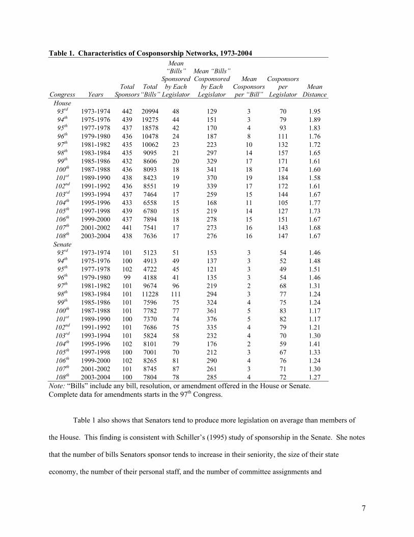
understand how institutional rules or artifacts in the data may drive some of the network measures. Table

1 presents some statistics about these networks. Notice that the number of sponsors varies only slightly

(less than 2%) from Congress to Congress due to deaths and retirements that occur between Congresses

and in some cases inactivity by a particular member. However, there are two fairly large and systematic

changes in the total number of bills sponsored that are worth noting.

First, prior to the 96th Congress there was a 25 cosponsor limit on all legislation in the House.

As a result, the number of bills sponsored in the 93rd - 95th Houses is about double the number of bills

sponsored in later years. These numbers are inflated because of the incidence of identical bills during this

period. However, this rule did not deter legislators who sought more support—it was not uncommon for

several identical versions of the same bill to be submitted, each with a different set of 25 cosponsors. In

1978 the House voted to remove the limit. Second, the Library of Congress Thomas database provides

complete data for all bills and resolutions since the 93rd Congress, but complete data for amendments is

not available until the 97th Congress. The number of amendments sometimes exceeds the number of bills

and resolutions in the Senate, helping to explain the substantial jump in total bills in the 97th Senate. It is

unlikely that either of these systematic features of the data will greatly affect comparability of the

cosponsorship networks between Congresses since legislators found a way around the institutional limit

on cosponsors in the House, and amendments in both the House and Senate are only rarely cosponsored.

7

Table 1. Characteristics of Cosponsorship Networks, 1973-2004

Congress Years Total

SponsorsTotal

“Bills”

Mean “Bills”

Sponsored by Each

Legislator

Mean “Bills” Cosponsored

by Each Legislator

Mean Cosponsors per “Bill”

Cosponsors per

Legislator Mean

Distance House 93rd 1973-1974 442 20994 48 129 3 70 1.95 94th 1975-1976 439 19275 44 151 3 79 1.89 95th 1977-1978 437 18578 42 170 4 93 1.83 96th 1979-1980 436 10478 24 187 8 111 1.76 97th 1981-1982 435 10062 23 223 10 132 1.72 98th 1983-1984 435 9095 21 297 14 157 1.65 99th 1985-1986 432 8606 20 329 17 171 1.61

100th 1987-1988 436 8093 18 341 18 174 1.60 101st 1989-1990 438 8423 19 370 19 184 1.58 102nd 1991-1992 436 8551 19 339 17 172 1.61 103rd 1993-1994 437 7464 17 259 15 144 1.67 104th 1995-1996 433 6558 15 168 11 105 1.77 105th 1997-1998 439 6780 15 219 14 127 1.73 106th 1999-2000 437 7894 18 278 15 151 1.67 107th 2001-2002 441 7541 17 273 16 143 1.68 108th 2003-2004 438 7636 17 276 16 147 1.67

Senate 93rd 1973-1974 101 5123 51 153 3 54 1.46 94th 1975-1976 100 4913 49 137 3 52 1.48 95th 1977-1978 102 4722 45 121 3 49 1.51 96th 1979-1980 99 4188 41 135 3 54 1.46 97th 1981-1982 101 9674 96 219 2 68 1.31 98th 1983-1984 101 11228 111 294 3 77 1.24 99th 1985-1986 101 7596 75 324 4 75 1.24

100th 1987-1988 101 7782 77 361 5 83 1.17 101st 1989-1990 100 7370 74 376 5 82 1.17 102nd 1991-1992 101 7686 75 335 4 79 1.21 103rd 1993-1994 101 5824 58 232 4 70 1.30 104th 1995-1996 102 8101 79 176 2 59 1.41 105th 1997-1998 100 7001 70 212 3 67 1.33 106th 1999-2000 102 8265 81 290 4 76 1.24 107th 2001-2002 101 8745 87 261 3 71 1.30 108th 2003-2004 100 7804 78 285 4 72 1.27

Note: “Bills” include any bill, resolution, or amendment offered in the House or Senate. Complete data for amendments starts in the 97th Congress.

Table 1 also shows that Senators tend to produce more legislation on average than members of

the House. This finding is consistent with Schiller’s (1995) study of sponsorship in the Senate. She notes

that the number of bills Senators sponsor tends to increase in their seniority, the size of their state

economy, the number of their personal staff, and the number of committee assignments and

8

chairmanships. Compared to members of the House, Senators tend to have been in politics longer, come

from larger districts with bigger economies, have 2 to 3 times more personal staff than House members,

and sit on and chair more committees since there are many fewer members to conduct business. In

contrast, the number of bills cosponsored by each legislator does not differ systematically by chamber—

the mean House member cosponsored 129 to 370 bills while the mean Senator cosponsored between 121

and 360 bills. Since there are more members of the House than the Senate, House bills tend to receive

more cosponsorships than Senate bills, but as a percent of the chamber the ranges are quite similar.

Using Cosponsorships to Connect Legislators

The cosponsorship networks do not merely yield insights into aggregate patterns of legislator

activity—they also contain a wealth of information about connections between individual legislators. In

the jargon of social network theory, each legislator represents a node in the cosponsorship network, and

we can draw a tie from each legislator who cosponsors a bill to the sponsor of that bill. These ties are

directed (asymmetric), because they reflect the cosponsoring legislator’s support of the sponsoring

legislator’s proposed legislation. Although below we will see that there is a significant amount of

reciprocal support between legislators, it is important to emphasize here that the direction of each tie

provides information about the direction in which support between legislators tends to flow.

There are many ways to measure how much total support a legislator receives in this network.

Perhaps the simplest is to identify the total number of bills sponsored by a given legislator and then count

all the legislators who have cosponsored at least one these bills. Table 1 shows that the average number

of unique cosponsors per legislator varies from 70 to 184 in the House and from 52 to 83 in the Senate.

Notice that although the absolute numbers of cosponsors per legislator tend to be higher in the House,

Senators tend to receive support from a much larger fraction of the total members in their chamber. There

are also some important changes over time. The average number of cosponsors per legislator reflects in

part the degree to which the average member is integrated into the network—when legislators have more

cosponsors it may indicate they are operating in an environment in which it is easier to obtain broad

9

support. Thus, it is particularly interesting that this value falls sharply for the 104th Congress when the

“Republican Revolution” caused a dramatic change in the partisan and seniority compositions of both

chambers.

Counting unique cosponsors is an important first step in understanding how connected a given

legislator is to the network. However, this method neglects information about the legislators who are

offering their support. Are the cosponsors themselves well-connected? If so, it might indicate that the

sponsor is more closely connected to the network than she would be if she was receiving cosponsorships

from less connected individuals. One way to incorporate this information is to calculate the shortest

cosponsorship distance, or geodesic, between each pair of legislators. A given sponsor has a distance of 1

between herself and all her cosponsors. She has a distance of 2 between herself and the set of all

legislators who cosponsored a bill that was sponsored by one of her cosponsors. One can repeat this

process for distances of 3, 4, and so on until the shortest paths are drawn for all legislators in the network.

The average distance from one legislator to all others thus gives us an idea of not only how much direct

support she receives, but how much support her supporters receive.

Figure 1 shows two examples of these distance calculations for the 108th House. Rep. Randy

“Duke” Cunningham received unique cosponsorships from 421 legislators, and thus had a distance of 1 to

Figure 1. Example of Cosponsorship Distance Between Legislators

10

each of them. The remaining 16 legislators to whom he had no direct connection were cosponsors on

bills sponsored by one of the 421 legislators to whom he did have a direct connection. These legislators

had a distance of 2. Thus the average distance between Cunningham and the other legislators in the

network was 1.04. At the other extreme, Harold Rogers received a direct cosponsorship by a single

individual—Rep. Zach Wamp. Wamp received support from three other individuals, who in turn

received support from 319 representatives. The remaining 114 individuals cosponsored at least one bill

by someone in the group of 319. Thus, Rogers had a distance of 1 to one legislator, 2 to 3 legislators, 3 to

319 legislators, and 4 to 114, for an average distance of 3.25.

Table 1 shows that the mean average distances for each chamber and Congress are quite short,

suggesting that legislative networks are very densely connected. In the Senate the average distance

ranges from 1.17 to 1.51 while in the House it ranges from 1.58 to 1.95. In other words, in the Senate the

average member is directly connected to nearly all the other Senators, while in the House the average

member tends to be indirectly connected through at most a single intermediary to all the other

Representatives. As suggested by studies of the legislative committee assignment network (Porter et al.

2005), the smaller and more powerful Senate appears to be more densely connected than the House.

Mutual Cosponsorship

The data clearly shows that the average legislator is supported directly or indirectly by the vast

majority of her peers. But to what extent do legislators reciprocate by supporting one another’s bills? To

answer this question, it will be useful to introduce some notation for describing individual relationships

within it. Let A be an n x n adjacency matrix representing all the cosponsorship ties in a network for a

given Congress and chamber such that 1ija = if the ith legislator cosponsors a bill by the jth legislator

and 0 otherwise. This network represents the set of unique cosponsorships and contains no information

about how often legislators cosponsor each other. To include this information, let Q be an n x n

11

Table 2. Mutual Cosponsorship Relationships Any Bill Total Number of Bills

Congress House Senate House Senate 93rd 0.17 0.23 0.23 0.39 94th 0.17 0.25 0.20 0.34 95th 0.17 0.21 0.19 0.33 96th 0.12 0.12 0.15 0.26 97th 0.14 0.17 0.22 0.27 98th 0.15 0.16 0.23 0.36 99th 0.14 0.19 0.21 0.34

100th 0.18 0.18 0.25 0.39 101st 0.15 0.17 0.24 0.39 102nd 0.15 0.26 0.14 0.30 103rd 0.17 0.19 0.23 0.34 104th 0.16 0.20 0.21 0.29 105th 0.16 0.19 0.24 0.36 106th 0.16 0.17 0.25 0.37 107th 0.17 0.17 0.29 0.47 108th 0.18 0.18 0.34 0.43

Note: Pearson Product Moment Correlations.

adjacency matrix representing all the cosponsorship ties in a network such that ijq is the total quantity of

bills sponsored by the jth legislator that are cosponsored by the ith legislator.

As noted earlier, cosponsorship is a directed relationship. The cosponsor of a bill is assumed to

be expressing support for the sponsor’s legislation, not the other way around. However, consistent with

earlier work (Burkett 1997), there appears to be a significant amount of mutual cosponsorship in the

network. Table 2 shows that legislators are more likely to cosponsor bills that are sponsored by those

who return the favor. The first two columns are simple correlations between and ij jia a i j∀ ≠ for the

House and Senate. In other words, how likely is it that legislator i has cosponsored at least one bill by

legislator j if legislator j has cosponsored at least one bill by legislator i? The next two columns are

simple correlations between and ij jiq q i j∀ ≠ for the House and Senate. In other words, how

correlated are the quantity of bills sponsored by legislator i and cosponsored by legislator j with the

quantity of bills sponsored by legislator j and cosponsored by legislator i?

12

In both chambers and across all years there appears to be significant tendency to engage in mutual

cosponsorship. Senators are somewhat more likely to reciprocate than members of the House. Moreover,

the higher correlations that result when we include information about the quantity of bills cosponsored

suggests that legislators who cosponsor a lot of bills by one legislator are likely to receive many

cosponsorships from the same legislator. The narrow range of variation in these correlations indicates

that norms of mutual cosponsorship have remained relatively stable over time in both bodies, though

some of the variation may carry implications for how these bodies function. For example, there appears

to be an increase in mutual cosponsorship in the 107th and 108th Congresses. It is not clear whether this is

due to an increase in cosponsorship activity between members with shared interests or the strategic

trading of support on different bills (logrolling). Either way, the significant and persistent tendency to

reciprocate suggests that cosponsorship is a way to build relationships with other legislators (Burkett

1997) and thus provides relevant information about their social network. But how can we use this

information to determine which legislators are best connected to the network?

Traditional Measures of Centrality

Social network theorists have described a variety of ways to use information about social ties to

make inferences about the relative importance of group members. Since we are interested in how

connected legislators are to other legislators in the cosponsorship network, I will focus on measures of

centrality. There are a number of ways to calculate centrality, and each has been shown to perform well

in identifying important individuals in social (Freeman, Borgatti, and White 1991) and epidemiological

networks (Rothenberg, Potterat, and Woodhouse 1995). The first and most obvious of these has already

been discussed—the total number of directed ties to an individual node reflects the degree to which that

node is supported by other nodes. Degree centrality (Proctor and Loomis 1951) or prestige scores, then,

are simply the total number of unique cosponsors that support each legislator: 1 2j j j njx a a a= + + + .

13

Burkett (1997) utilizes this measure to show that there is no relationship between seniority and prestige in

the Senate.

Other measures of centrality look beyond direct cosponsorship ties. As noted above, it is possible

to measure the social distance between any pair of individuals in the network by finding one’s

cosponsors, the cosponsors of one’s cosponsors, and so on. Closeness centrality (Sabidussi 1966) is the

inverse of the average distance from one legislator to all other legislators. If we let ijδ denote the shortest

distance from i to j, then ( ) ( )1 21j j j njx n δ δ δ= − + + + .

A third measure, betweenness centrality (Freeman 1977), identifies the extent to which an

individual in the network is critical for passing support from one individual to another. Some legislators

may, for example, receive support from several legislators and give it to several other legislators, acting

as a bridge between them. Once we identify each of the shortest paths in the network, we can count the

number of these paths that pass through each legislator. The higher this number the greater the effect

would be on the total average distance for the network if this person were removed (Wasserman and Faust

1994). If we let ikσ represent the number of paths from legislator i to legislator k, and ijkσ represent the

number of paths from legislator i to legislator k that pass through legislator j, then ijkj

i j k ik

xσσ≠ ≠

= ∑ .

A fourth measure, eigenvector centrality (Bonacich 1972), assumes that the centrality of a given

individual is an increasing function of the centralities of all the individuals that support her. While this is

an intuitive way to think about which legislators might be better connected, it yields a practical

problem—how do we simultaneously estimate the centrality of a given legislator and the centralities of

the legislators who cosponsor her? Let x be a vector of centrality scores so that each legislator’s centrality

jx is the sum of the centralities of the legislators who cosponsor her legislation:

1 1 2 2j j j nj nx a x a x a x= + + + . This yields n equations which we can represent in matrix format as

Tx A x= . It is unlikely that these equations have a nonzero solution, so Bonacich (1972) suggests an

14

important modification. Suppose the centrality of a legislator is proportional to instead of equal to the

centrality of the legislators who cosponsor one of her bills. Then 1 1 2 2i i i ni nx a x a x a xλ = + + + which

can be represented as Tx A xλ = . The vector of centralities x can now be computed since it is an

eigenvector of the eigenvalue λ. Although there are n nonzero solutions to this set of equations, in

practice the eigenvector corresponding to the principal eigenvalue is used because it maximizes the

accuracy with which the associated eigenvector can reproduce the adjacency matrix (Bonacich 1987).

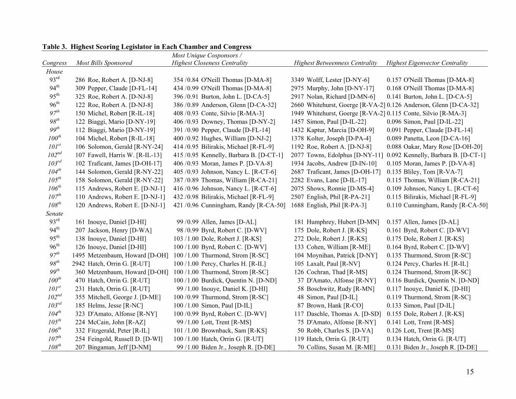
Who is the most central legislator? Table 3 presents the scores and names of the top performers

on each of these traditional measures of importance by chamber and Congress. The first two columns

show the total number of bills sponsored and the total number of unique cosponsors (degree centrality).

These values should have a strong relationship with other measures of centrality since they reflect the

total number of opportunities for cosponsorship and the breadth of direct support an individual receives

from other legislators. Column two also presents closeness centrality scores. Although degree centrality

and closeness centrality scores do not perfectly correlate, they are similar enough in these networks that

they generate the exact same set of names for the highest score in each chamber and Congress. This is

because legislators are so densely connected in these networks that direct support makes up a very large

part of the closeness centrality score, which is based on both direct and indirect support.

Columns three and four of Table 3 show the top legislators based on betweenness and eigenvector

centrality scores. Notice that there is a strong correspondence between the names in the eigenvector

centrality list and the closeness centrality list, but the betweenness list is quite different. All of the

centrality scores produce names that are familiar to students of American politics. They include majority

and minority leaders (O’Neill, Byrd, Dole, Daschle, and Lott), numerous committee chairs, and

individuals that would later run for higher office or otherwise be involved in presidential politics.

15

Table 3. Highest Scoring Legislator in Each Chamber and Congress

Congress Most Bills Sponsored Most Unique Cosponsors / Highest Closeness Centrality Highest Betweenness Centrality

Highest Eigenvector Centrality

House 93rd 286 Roe, Robert A. [D-NJ-8] 354 /0.84 O'Neill Thomas [D-MA-8] 3349 Wolff, Lester [D-NY-6] 0.157 O'Neill Thomas [D-MA-8] 94th 309 Pepper, Claude [D-FL-14] 434 /0.99 O'Neill Thomas [D-MA-8] 2975 Murphy, John [D-NY-17] 0.168 O'Neill Thomas [D-MA-8] 95th 325 Roe, Robert A. [D-NJ-8] 396 /0.91 Burton, John L. [D-CA-5] 2917 Nolan, Richard [D-MN-6] 0.141 Burton, John L. [D-CA-5] 96th 122 Roe, Robert A. [D-NJ-8] 386 /0.89 Anderson, Glenn [D-CA-32] 2660 Whitehurst, Goerge [R-VA-2] 0.126 Anderson, Glenn [D-CA-32] 97th 150 Michel, Robert [R-IL-18] 408 /0.93 Conte, Silvio [R-MA-3] 1949 Whitehurst, Goerge [R-VA-2] 0.115 Conte, Silvio [R-MA-3] 98th 122 Biaggi, Mario [D-NY-19] 406 /0.93 Downey, Thomas [D-NY-2] 1457 Simon, Paul [D-IL-22] 0.096 Simon, Paul [D-IL-22] 99th 112 Biaggi, Mario [D-NY-19] 391 /0.90 Pepper, Claude [D-FL-14] 1432 Kaptur, Marcia [D-OH-9] 0.091 Pepper, Claude [D-FL-14]

100th 104 Michel, Robert [R-IL-18] 400 /0.92 Hughes, William [D-NJ-2] 1378 Kolter, Joseph [D-PA-4] 0.089 Panetta, Leon [D-CA-16] 101st 106 Solomon, Gerald [R-NY-24] 414 /0.95 Bilirakis, Michael [R-FL-9] 1192 Roe, Robert A. [D-NJ-8] 0.088 Oakar, Mary Rose [D-OH-20] 102nd 107 Fawell, Harris W. [R-IL-13] 415 /0.95 Kennelly, Barbara B. [D-CT-1] 2077 Towns, Edolphus [D-NY-11] 0.092 Kennelly, Barbara B. [D-CT-1] 103rd 102 Traficant, James [D-OH-17] 406 /0.93 Moran, James P. [D-VA-8] 1934 Jacobs, Andrew [D-IN-10] 0.105 Moran, James P. [D-VA-8] 104th 144 Solomon, Gerald [R-NY-22] 405 /0.93 Johnson, Nancy L. [R-CT-6] 2687 Traficant, James [D-OH-17] 0.135 Bliley, Tom [R-VA-7] 105th 158 Solomon, Gerald [R-NY-22] 387 /0.89 Thomas, William [R-CA-21] 2282 Evans, Lane [D-IL-17] 0.115 Thomas, William [R-CA-21] 106th 115 Andrews, Robert E. [D-NJ-1] 416 /0.96 Johnson, Nancy L. [R-CT-6] 2075 Shows, Ronnie [D-MS-4] 0.109 Johnson, Nancy L. [R-CT-6] 107th 110 Andrews, Robert E. [D-NJ-1] 432 /0.98 Bilirakis, Michael [R-FL-9] 2507 English, Phil [R-PA-21] 0.115 Bilirakis, Michael [R-FL-9] 108th 120 Andrews, Robert E. [D-NJ-1] 421 /0.96 Cunningham, Randy [R-CA-50] 1688 English, Phil [R-PA-3] 0.110 Cunningham, Randy [R-CA-50]

Senate 93rd 161 Inouye, Daniel [D-HI] 99 /0.99 Allen, James [D-AL] 181 Humphrey, Hubert [D-MN] 0.157 Allen, James [D-AL] 94th 207 Jackson, Henry [D-WA] 98 /0.99 Byrd, Robert C. [D-WV] 175 Dole, Robert J. [R-KS] 0.161 Byrd, Robert C. [D-WV] 95th 138 Inouye, Daniel [D-HI] 103 /1.00 Dole, Robert J. [R-KS] 272 Dole, Robert J. [R-KS] 0.175 Dole, Robert J. [R-KS] 96th 126 Inouye, Daniel [D-HI] 100 /1.00 Byrd, Robert C. [D-WV] 133 Cohen, William [R-ME] 0.164 Byrd, Robert C. [D-WV] 97th 1495 Metzenbaum, Howard [D-OH] 100 /1.00 Thurmond, Strom [R-SC] 104 Moynihan, Patrick [D-NY] 0.135 Thurmond, Strom [R-SC] 98th 2942 Hatch, Orrin G. [R-UT] 100 /1.00 Percy, Charles H. [R-IL] 105 Laxalt, Paul [R-NV] 0.124 Percy, Charles H. [R-IL] 99th 360 Metzenbaum, Howard [D-OH] 100 /1.00 Thurmond, Strom [R-SC] 126 Cochran, Thad [R-MS] 0.124 Thurmond, Strom [R-SC]

100th 470 Hatch, Orrin G. [R-UT] 100 /1.00 Burdick, Quentin N. [D-ND] 37 D'Amato, Alfonse [R-NY] 0.116 Burdick, Quentin N. [D-ND] 101st 231 Hatch, Orrin G. [R-UT] 99 /1.00 Inouye, Daniel K. [D-HI] 58 Boschwitz, Rudy [R-MN] 0.117 Inouye, Daniel K. [D-HI] 102nd 355 Mitchell, George J. [D-ME] 100 /0.99 Thurmond, Strom [R-SC] 48 Simon, Paul [D-IL] 0.119 Thurmond, Strom [R-SC] 103rd 185 Helms, Jesse [R-NC] 100 /1.00 Simon, Paul [D-IL] 87 Brown, Hank [R-CO] 0.133 Simon, Paul [D-IL] 104th 323 D'Amato, Alfonse [R-NY] 100 /0.99 Byrd, Robert C. [D-WV] 117 Daschle, Thomas A. [D-SD] 0.155 Dole, Robert J. [R-KS] 105th 224 McCain, John [R-AZ] 99 /1.00 Lott, Trent [R-MS] 75 D'Amato, Alfonse [R-NY] 0.141 Lott, Trent [R-MS] 106th 332 Fitzgerald, Peter [R-IL] 101 /1.00 Brownback, Sam [R-KS] 50 Robb, Charles S. [D-VA] 0.126 Lott, Trent [R-MS] 107th 254 Feingold, Russell D. [D-WI] 100 /1.00 Hatch, Orrin G. [R-UT] 119 Hatch, Orrin G. [R-UT] 0.134 Hatch, Orrin G. [R-UT] 108th 207 Bingaman, Jeff [D-NM] 99 /1.00 Biden Jr., Joseph R. [D-DE] 70 Collins, Susan M. [R-ME] 0.131 Biden Jr., Joseph R. [D-DE]

16

Connectedness: An Alternative Measure

Although the traditional measures of centrality appear to generate some plausible candidates for

the title “best-connected legislator,” none of these takes advantage of two other pieces of information that

might be helpful for determining the strength of social relationships that exist in the network. First, we

have information about the total number of cosponsors c on each bill . The binary indicator ija

assigns a connection from legislator i to j, regardless of whether a bill has 1 cosponsor or 100. However,

legislators probably recruit first those legislators to whom they are most closely connected. Moreover, as

the total number of cosponsors increases, it becomes more likely that the cosponsor is recruited by an

intermediary other than the sponsor, increasing the possibility that there is no direct connection at all.

Thus bills with fewer total cosponsors probably provide more reliable information about the real social

connections between two legislators than bills with many cosponsors (Burkett 1997). This relationship

might take several different functional forms, but I assume a simple one: the strength of the connection

between i and j on a given bill is posited to be 1/ c .

Second, we have information about the total number of bills sponsored by j that are cosponsored

by i. Legislators who frequently cosponsor bills by the same sponsor are more likely to have a real social

relationship with that sponsor than those that cosponsor only a few times. We have already seen that the

quantity of bills cosponsored ijq is a better predictor of mutual cosponsorship than the simple binary

indicator ija . This suggests that we might use information about the quantity of bills to denote the

strength of the tie between i and j. To incorporate this information with the assumption about the effect of

the number of cosponsors into a measure of connectedness, let ija be a binary indicator that is 1 if

legislator i cosponsors a given bill that is sponsored by legislator j, and 0 otherwise. Then the weighted

quantity of bills cosponsored ijw will be the sum ij ijw a c=∑ .

This measure is closely related to the weighted measure used by Newman (2001b) to find the best

connected scientist in the scientific coauthorship network, which assumes that tie strength is proportional

17

to the number of papers two scholars coauthor together and inversely proportional to the number of other

coauthors on each paper. However, ties in the cosponsorship network are directed. This means that

unlike the scientific coauthorship network which has symmetric weights ij jiw w= , the weights in the

cosponsorship network are not symmetric: ij jiw w≠ .

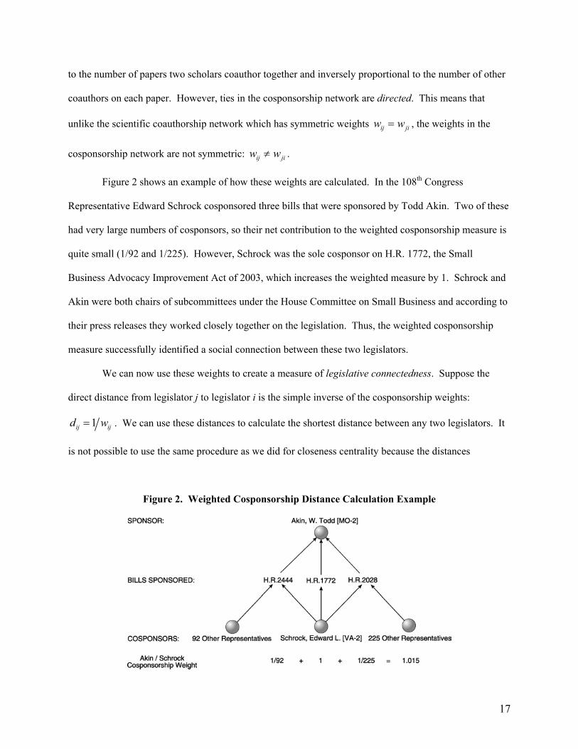
Figure 2 shows an example of how these weights are calculated. In the 108th Congress

Representative Edward Schrock cosponsored three bills that were sponsored by Todd Akin. Two of these

had very large numbers of cosponsors, so their net contribution to the weighted cosponsorship measure is

quite small (1/92 and 1/225). However, Schrock was the sole cosponsor on H.R. 1772, the Small

Business Advocacy Improvement Act of 2003, which increases the weighted measure by 1. Schrock and

Akin were both chairs of subcommittees under the House Committee on Small Business and according to

their press releases they worked closely together on the legislation. Thus, the weighted cosponsorship

measure successfully identified a social connection between these two legislators.

We can now use these weights to create a measure of legislative connectedness. Suppose the

direct distance from legislator j to legislator i is the simple inverse of the cosponsorship weights:

1ij ijd w= . We can use these distances to calculate the shortest distance between any two legislators. It

is not possible to use the same procedure as we did for closeness centrality because the distances

Figure 2. Weighted Cosponsorship Distance Calculation Example

18

between each pair of legislators are not uniform—sometimes the shortest distance will be through several

legislators who are closely connected instead of fewer legislators who are only distantly connected.

Dijkstra’s algorithm (Cormen et al. 2001) allows us to find the shortest distance between each pair of

legislators using the following steps: 1) Starting with legislator j, identify from a list of all other

legislators the closest legislator i. 2) Replace each of the distances kjd with ( )min ,kj ki ijd d d+ . 3)

Remove legislator i from the list and repeat until there are no more legislators on the list. Once we repeat

this procedure for each legislator the result is a matrix of shortest distances between each pair of

legislators in the whole network. Connectedness is the inverse of the average of these distances from all

other legislators to legislator j: ( ) ( )1 21 j j njn d d d− + + + .

Table 4 shows a list of the best connected legislator in each chamber and Congress. Just like the

centrality measures, the connectedness measure identifies several majority and minority leaders and

committee chairs. To illustrate some of the relationships behind these rankings, column two shows the

strongest sponsor / cosponsor weight identified within each chamber and Congress and column three

identifies the specific relationship between these two individuals. The sources of these relationships can

be divided into four categories: institutional, regional, issue-based, and personal.

Institutional relationships dominate both chambers. Most of the strongest relationships in the

House are between committee chairs and ranking members, while in the Senate they are between majority

and minority leaders. Intuitively, it makes sense that party leaders in each committee (including the

“committee of the whole” in the Senate) would be strongly connected since they spend a great deal of

time together and probably expend a lot of effort negotiating for each other’s support. Consistent with

prior work (Pellegrini and Grant 1999), regional relationships also appear to be important despite partisan

differences. Not only are many of the most strongly connected legislators from the same state—in the

House they are often from contiguous districts. This suggests that politicians may belong to regional or

state organizations or may have roots in local politics that cause them to be more likely to have made

prior social contacts with one another. Alternatively, they may share similar interests because their

19

Table 4. Best Connected Legislator and Strongest Sponsor / Cosponsor Relationship in Each Chamber and Congress Congress Best Connected Legislator Strongest Sponsor / Cosponsor Relation Relationship

House 93rd 0.44 Koch, Edward [D-NY-18] 69 Staggers, Harley [D-WV-2] / Devine, Samuel [R-OH-12] Commerce Chair, Ranking Member 94th 0.57 Pepper, Claude [D-FL-14] 72 Price, Melvin [D-IL-21] / Wilson, Robert [R-CA-41] Armed Services Chair, Ranking Member 95th 0.60 Pepper, Claude [D-FL-14] 51 Price, Melvin [D-IL-21] / Wilson, Robert [R-CA-41] Armed Services Chair, Ranking Member 96th 0.31 Pepper, Claude [D-FL-14] 58 Price, Melvin [D-IL-21] / Wilson, Robert [R-CA-41] Armed Services Chair, Ranking Member 97th 0.27 Montgomery, G. [D-MS-3] 29 Price, Melvin [D-IL-21] / Dickinson, William [R-AL-2] Armed Services Chair, Ranking Member 98th 0.27 Roe, Robert A. [D-NJ-8] 30 Price, Melvin [D-IL-21] / Dickinson, William [R-AL-2] Armed Services Chair, Ranking Member 99th 0.26 Breaux, John [D-LA-7] 16 Montgomery, G. [D-MS-3] / Hammerschmidt, J. [R-AR-3] Veterans Affairs Chair, Ranking Member

100th 0.25 Waxman, Henry A. [D-CA-29] 57 Montgomery, G. [D-MS-3] / Solomon, Gerald [R-NY-24] Veterans Affairs Chair, Ranking Member 101st 0.28 Stark, Fortney Pete [D-CA-9] 23 Schulze, Richard T. [R-PA-5] / Yatron, Gus [D-PA-6] Contiguous Districts 102nd 0.27 Fawell, Harris W. [R-IL-13] 14 Hughes, William [D-NJ-2] / Moorhead, Carlos [R-CA-22] Courts and Intellectual Property Chair, Ranking Member 103rd 0.22 Waxman, Henry A. [D-CA-29] 8 Hughes, William [D-NJ-2] / Moorhead, Carlos [R-CA-27] Courts and Intellectual Property Chair, Ranking Member 104th 0.24 Traficant, James [D-OH-17] 7 Moorhead, Carlos [R-CA-27] / Schroeder, Pat [D-CO-1] Courts and Intellectual Property Chair, Ranking Member 105th 0.22 Gilman, Benjamin [R-NY- 20] 7 Ensign, John E. [R-NV-1] / Gibbons, Jim [R-NV-2] Contiguous Districts 106th 0.28 McCollum, Bill [R-FL-8] 10 Shuster, Bud [R-PA-9] / Oberstar, James L. [D-MN-8] Transportation Chair, Ranking Member 107th 0.24 Young, Don [R-AK] 11 DeMint, Jim [R-SC-4] / Myrick, Sue [R-NC-9] (Nearly) Contiguous Districts, Repub. Study Committee 108th 0.28 Saxton, Jim [R-NJ-3] 14 Ney, Robert W. [R-OH-18] / Larson, John B. [D-CT-1] House Administration Chair, Ranking

Senate 93rd 0.94 Jackson, Henry [D-WA] 65 Magnuson, Warren [D-WA] / Cotton, Norris [R-NH] Commerce Chair, Ranking Member 94th 1.12 Moss, Frank [D-UT] 139 Jackson, Henry [D-WA] / Fannin, Paul [R-AZ] Interior and Insular Affairs Chair, Ranking Member 95th 0.90 Dole, Robert J. [R-KS] 33 Inouye, Daniel [D-HI] / Matsunaga, Spark [D-HI] Same State 96th 0.84 Dole, Robert J. [R-KS] 24 Byrd, Robert [D-WV] / Baker, Howard [R-TN] Majority, Minority Leader 97th 0.91 Heinz, Henry [R-PA] 34 Inouye, Daniel [D-HI] / Matsunaga, Spark [D-HI] Same State 98th 1.28 Hatch, Orrin G. [R-UT] 63 Baker, Howard [R-TN] / Byrd, Robert [D-WV] Majority, Minority Leader 99th 1.37 Thurmond, Strom [R-SC] 109 Cranston, Alan [D-CA] / Wilson, Pete [R-CA] Same State

100th 1.46 Cranston, Alan [D-CA] 70 Byrd, Robert [D-WV] / Dole, Robert J. [R-KS] Majority, Minority Leader 101st 1.39 Kennedy, Edward M. [D-MA] 77 Mitchell, George J. [D-ME] / Dole, Robert J. [R-KS] Majority, Minority Leader 102nd 1.23 Mitchell, George J. [D-ME] 179 Mitchell, George J. [D-ME] / Sasser, Jim [D-TN] Federal Housing Reform 103rd 1.20 Mitchell, George J. [D-ME] 59 Mitchell, George J. [D-ME] / Dole, Robert J. [R-KS] Majority, Minority Leader 104th 1.58 Dole, Robert J. [R-KS] 38 Dole, Robert J. [R-KS] / Daschle, Thomas A. [D-SD] Majority, Minority Leader 105th 1.36 McCain, John [R-AZ] 40 Lott, Trent [R-MS] / Daschle, Thomas A. [D-SD] Majority, Minority Leader 106th 1.36 Hatch, Orrin G. [R-UT] 104 Hutchison, Kay Bailey [R-TX] / Brownback, Sam [R-KS] Marriage Penalty Relief and Bankruptcy Reform 107th 1.61 Feingold, Russell D. [D-WI] 53 McCain, John [R-AZ] / Gramm, Phil [R-TX] Personal 108th 1.43 McCain, John [R-AZ] 50 Frist, Bill [R-TN] / Daschle, Thomas A. [D-SD] Majority, Minority Leader

20

constituents have similar geographic characteristics. Either way, being from the same place seems to

increase the likelihood that legislators will cosponsor one another’s legislation.

Some pairs of legislators work closely together because they are drawn to the same issues. For

example, Representatives Jim DeMint and Sue Myrick both belong to the Republican Study Committee;

Senators George Mitchell and Jim Sasser worked together on Federal Housing Reform and Senators Kay

Bailey Hutchinson and Sam Brownback worked together extensively on marriage penalty relief and

bankruptcy reform. This finding is consistent with prior work which suggests that ideological similarity

increases the probability of mutual cosponsorship (Burkett 1997). Finally, some relationships might be

best described as personal. For example, Senator John McCain chaired Senator Phil Gramm’s 1996

Presidential campaign, but McCain has told the media that they have been friends since 1982 when they

served together in the House (McGrory 1995). It is possible that friendship is at the core of some of these

other relationships, but this may be difficult to evaluate if politicians choose to keep this information

private.

Connectedness in the 108th Congress

What are the legislative characteristics of the legislators who receive high connectedness scores?

Table 5 provides a list of the top 20 most connected legislators for the 108th House and Senate and shows

how many bills each of them sponsored and the total number of legislators who cosponsored at least one

of their bills. Notice that these general indicators of legislative activity are very important—all but five

legislators sponsored more bills than average and received more cosponsorships than average.

Representative Ron Paul is ranked 2nd but he was cosponsored by only 123 other legislators

compared to an average of 147 in the House. Although he clearly had difficulty soliciting broad support,

he made up for it with legislative productivity—he ranked 3rd in the House for the number of bills

sponsored. Representative Jeb Bradley who is ranked 15th for connectedness scored below average on

both sponsorships and cosponsorships. However, the cosponsors who supported him are themselves

ranked very highly—four of his eight closest supporters (Sensenbrenner, Paul, English, and Evans) are

21

Table 5. Best Connected Legislators in 108th Senate and House

Rank Best Connected Representatives “Bills”

SponsoredUnique

Cosponsors Best Connected Senators “Bills”

SponsoredUnique

Cosponsors1 Saxton, Jim [R-NJ-3] 40 258 McCain, John [R-AZ] 189 80 2 Paul, Ron [R-TX-14] 76 123 Hatch, Orrin G. [R-UT] 133 97 3 Smith, Christopher H. [R-NJ-4] 57 336 Bingaman, Jeff [D-NM] 207 89 4 Millender-McDonald, Juanita [D-CA-37] 50 205 Grassley, Charles E. [R-IA] 156 97 5 Rangel, Charles B. [D-NY-15] 77 219 Feingold, Russell D. [R-WI] 121 64 6 Sensenbrenner, F. James, Jr. [R-WI-5] 45 339 Kyl, Jon [R-AZ] 114 99 7 Maloney, Carolyn B. [D-NY-14] 66 225 Kennedy, Edward [D-MA] 130 78 8 Andrews, Robert E. [D-NJ-1] 120 194 Leahy, Patrick J. [D-VT] 132 85 9 King, Peter T. [R-NY-3] 40 376 Schumer, Charles [D-NY] 166 99

10 Young, Don [R-AK] 60 251 Domenici, Pete V. [R-NM] 108 97 11 Houghton, Amo [R-NY-29] 35 384 Feinstein, Dianne [D-CA] 145 95 12 Camp, Dave [R-MI-4] 36 355 Snowe, Olympia J. [R-ME] 137 94 13 DeLay, Tom [R-TX-22] 35 190 Clinton, Hillary [D-NY] 138 90 14 Filner, Bob [D-CA-51] 44 269 Frist, Bill [R-TN] 157 99 15 Bradley, Jeb [R-NH-1] 15 81 Collins, Susan M. [R-ME] 104 92 16 English, Phil [R-PA-3] 61 402 Voinovich, George [R-OH] 96 65 17 Simmons, Rob [R-CT-2] 26 187 Boxer, Barbara [D-CA] 137 93 18 Evans, Lane [D-IL-17] 27 216 Daschle, Thomas A. [D-SD] 125 77 19 Kucinich, Dennis J. [D-OH-10] 32 88 DeWine, Michael [R-OH] 90 94 20 Tancredo, Thomas G. [R-CO-6] 38 192 Durbin, Richard J. [D-IL] 122 79

House Average 17 147 Senate Average 78 72

ranked in the top 20 for connectedness. Similarly, Representative Dennis Kucinich had a below-average

number of cosponsors but managed to gain close support from Representatives Charles Rangel, Steve

LaTourette (ranked 21st), Luis Guttierez (ranked 25th), Jerold Nadler (ranked 26th) and John Conyers

(ranked 34th). On the Senate side, Russell Feingold and John Voinovich were both ranked in the top 20

but had a below average number of cosponsors. Voinovich’s two closest supporters are both in the top 20

(DeWine and Collins), as are three of Feingold’s four closest supporters (Leahy, Collins, and Durbin).

Thus, connectedness is not just about sponsoring a lot of bills and writing a lot of “Dear

Colleague” letters—it also matters who one convinces to sign on to the legislation. Figures 3 and 4

illustrate graphically the difference in the strength of ties between the 20 most connected and 20 least

connected legislators in each branch. Each arrow shows a cosponsorship relation pointing to the sponsor,

and to simplify the graph relationships to members outside the top or bottom 20 are not shown. Darker

arrows indicate stronger connections (higher values of ijw ). This visual interpretation of the data makes

22

Figure 3. Most and Least Connected Legislators in the 108th House

Note: These graphs only show connections among the 20 most connected (Top 20) and among the 20 least connected (Bottom 20). Connections between these two groups and to the other legislators in the 108th House are not shown. Graphs drawn using Pajek (de Nooy, Mrvar, and Batagelj 2005).

23

Figure 4. Most and Least Connected Legislators in the 108th Senate

Note: These graphs only show connections among the 20 most connected (Top 20) and among the 20 least connected (Bottom 20). Connections between these two groups and to the other legislators in the 108th Senate are not shown. Graphs drawn using Pajek (de Nooy, Mrvar, and Batagelj 2005).

24

clear the dramatic difference in cosponsorship activity between the most and least connected legislators.

It also helps illustrate how much more densely connected the Senate cosponsorship network is than the

House.

Connectedness, Centrality, and Legislative Influence

So far the connectedness measure has been shown to be reliable, yielding similar results in

different chambers and Congresses. It has also been shown to have face validity—the measure seems to

identify party leaders, committee chairs, and other well-connected people in the legislative network.

However, the same is true for the traditional centrality measures. To what extent is the connectedness

measure externally valid, and how does it compare to the alternatives? One way to test the external

validity of the connectedness measure is to compare it to measures of legislative influence. Legislators

who are able to elicit support in the cosponsorship network because they are broadly connected or well-

connected to other important legislators ought to be better able to shape the policies that emerge from

their chamber. But how do we measure this capacity?

The most widely used measure of legislative influence is the number of successful floor

amendments (Hall 1992; Sinclair 1989; Smith 1989; Weingast 1991). In particular, Hall (1992) argues

that the more amendments one manages to pass on the floor, the more direct influence one has on the

legislative process. Amendments are used instead of bills and resolutions because they tend to reflect

more specific changes to a bill that are less susceptible to deviations from the sponsor’s original intent.

Also, the number of amendments passed is used as a measure instead of the success rate because of the

problem of cross-cutting tendencies—more influential legislators who have a better chance of getting

things to pass probably propose more amendments, which reduces their success rate. Finally, one might

worry that this measure of legislative influence is not completely external to measures derived from the

cosponsorship network, since amendments themselves may be cosponsored. However, cosponsored

amendments make up only a very small portion of the data, are exceedingly rare in the House (there were

19 total from 1973-2004), and their exclusion does not alter substantive results.

25

Table 6. A Comparison of Connectedness and Centrality Measures in Each Congress

Closeness Betweenness Eigenvector Correlation Between Connectedness and

Connectedness Centrality Centrality Centrality Closeness Betweenness EigenvectorCongress Mean S.D. Mean S.D. Mean S.D. Mean S.D. Centrality Centrality Centrality

House 93rd 0.24 0.07 0.53 0.08 397 460 0.035 0.033 0.60 0.49 0.67 94th 0.26 0.08 0.54 0.08 371 431 0.036 0.031 0.51 0.44 0.59 95th 0.28 0.09 0.56 0.08 345 409 0.037 0.030 0.48 0.40 0.50 96th 0.17 0.06 0.58 0.08 319 367 0.038 0.029 0.31 0.30 0.34 97th 0.17 0.05 0.60 0.10 305 335 0.038 0.028 0.23 0.23 0.27 98th 0.16 0.05 0.63 0.11 274 275 0.039 0.028 0.30 0.25 0.30 99th 0.15 0.05 0.64 0.11 256 230 0.040 0.026 0.25 0.25 0.26 100th 0.15 0.05 0.64 0.11 255 230 0.040 0.025 0.31 0.22 0.31 101st 0.17 0.05 0.65 0.11 250 211 0.041 0.025 0.33 0.28 0.36 102nd 0.15 0.05 0.64 0.11 259 257 0.040 0.026 0.32 0.28 0.34 103rd 0.14 0.04 0.61 0.10 282 286 0.038 0.028 0.35 0.31 0.38 104th 0.13 0.05 0.58 0.08 320 370 0.036 0.031 0.26 0.29 0.28 105th 0.13 0.04 0.59 0.09 309 340 0.038 0.029 0.40 0.36 0.43 106th 0.16 0.05 0.62 0.10 288 259 0.040 0.026 0.42 0.35 0.46 107th 0.16 0.04 0.61 0.09 294 288 0.040 0.026 0.35 0.34 0.37 108th 0.17 0.05 0.61 0.09 292 271 0.040 0.026 0.30 0.28 0.33

Senate 93rd 0.61 0.15 0.70 0.11 46 33 0.091 0.040 0.57 0.54 0.57 94th 0.64 0.16 0.70 0.12 47 34 0.091 0.042 0.62 0.53 0.64 95th 0.57 0.13 0.68 0.11 52 43 0.088 0.043 0.46 0.49 0.47 96th 0.52 0.13 0.71 0.13 45 32 0.090 0.043 0.51 0.41 0.51 97th 0.62 0.13 0.79 0.13 31 19 0.094 0.034 0.43 0.37 0.40 98th 0.81 0.19 0.83 0.12 24 13 0.097 0.024 0.65 0.19 0.61 99th 0.86 0.20 0.83 0.12 24 16 0.095 0.029 0.61 0.31 0.58 100th 0.87 0.21 0.87 0.11 17 8 0.097 0.021 0.48 0.48 0.44 101st 0.92 0.20 0.87 0.12 17 8 0.098 0.022 0.47 0.35 0.43 102nd 0.84 0.18 0.85 0.12 21 9 0.096 0.026 0.54 0.57 0.50 103rd 0.77 0.18 0.79 0.13 30 16 0.094 0.031 0.56 0.45 0.56 104th 0.88 0.17 0.73 0.11 41 23 0.093 0.033 0.46 0.52 0.42 105th 0.89 0.18 0.77 0.12 32 15 0.096 0.029 0.40 0.46 0.39 106th 0.97 0.17 0.82 0.12 24 11 0.096 0.026 0.47 0.43 0.46 107th 1.05 0.24 0.79 0.12 30 17 0.096 0.027 0.34 0.38 0.37 108th 1.04 0.19 0.81 0.12 27 14 0.096 0.027 0.48 0.41 0.46

26

Table 6 provides information about the means and standard deviations of the connectedness and

centrality measures for comparison. It also shows simple correlations between these measures by

chamber and Congress. Not surprisingly, all of the correlations are positive, suggesting that

connectedness and centrality scores overlap somewhat in what they are measuring. Although I show

values for all Congresses, I will only be able to test external validity for the 97th Congress and later, since

that is when the Library of Congress Thomas database starts keeping track of all amendment activity in

the House and Senate.

The number of amendments passed is a count variable starting at 0, so Poisson regression might

be a natural choice for modeling the relationship with connectedness and centrality covariates. However,

the Poisson functional form implies the restrictive assumption that the variance equals the mean. Instead,

I use negative binomial regression which estimates an additional parameter that permits the variance to

differ from the mean. Although I do not report them in order to save space, estimates for this parameter

are always significantly different from one, implying that the true functional form is not Poisson.

Table 7 shows the results of separate bivariate regressions of the number of amendments passed

on each measure for each chamber and Congress. The table also shows an effect size for each estimate,

reflecting the percent increase in the number of amendments passed resulting from a one standard

deviation increase in the measure. For example, the regression results in the upper left of the table for

connectedness in the 97th House suggest that a one standard deviation increase in connectedness for a

given legislator would increase the number of amendments passed by that legislator by 33%. Another

way to think about these results is that we can expect a legislator ranked at the 95th percentile for

connectedness to pass 41.33 3.13= times more amendments than a legislator ranked at the 5th percentile.

This exercise is repeated 96 times for each combination of chamber, Congress, and measure. In

the center row and at the bottom of the table I also report results for regressions that pool the data from all

Congresses by chamber. These results show that a one standard deviation increase in connectedness in

the House increases the number of amendments passed by 54%, compared to 40% for closeness, 32% for

27

Table 7. Bivariate Relationship Between Connectedness, Centrality Measures, and the Number of Amendments Passed by Each Legislator in Each Congress

Dependent Variable: Number of Amendments Passed Independent Variables:

Connectedness Closeness Centrality Betweenness Centrality Eigenvector Centrality

Coef. S.E. p AIC Effect Size

Coef. S.E. p AIC

Effect Size

Coef. S.E. p AIC

Effect Size Coef. S.E. p AIC

Effect Size

House 97th 5.85 1.51 0.00 1373 33% 2.49 0.70 0.00 1373 28% 0.51 0.20 0.01 1380 19% 9.19 2.47 0.00 1372 29 98th 7.76 1.36 0.00 1432 50 2.71 0.58 0.00 1445 36 0.56 0.24 0.02 1461 17 10.83 2.39 0.00 1446 35 99th 9.27 1.49 0.00 1543 53 3.04 0.59 0.00 1555 40 1.52 0.27 0.00 1555 42 13.58 2.56 0.00 1554 41 100th 9.24 1.64 0.00 1283 57 2.05 0.67 0.00 1306 25 0.99 0.31 0.00 1306 25 10.41 3.03 0.00 1304 29 101st 12.89 1.79 0.00 1297 85 3.32 0.67 0.00 1329 45 1.57 0.35 0.00 1333 39 15.75 3.12 0.00 1328 47 102nd 13.31 2.00 0.00 1217 84 3.09 0.71 0.00 1249 40 1.32 0.29 0.00 1250 40 15.45 3.07 0.00 1243 49 103rd 17.58 2.56 0.00 1223 89 5.15 0.75 0.00 1224 69 1.58 0.26 0.00 1233 57 18.22 2.85 0.00 1230 66 104th 9.93 1.53 0.00 1349 60 6.11 0.70 0.00 1323 67 1.03 0.15 0.00 1340 47 17.10 1.89 0.00 1320 70 105th 14.00 1.97 0.00 1175 80 3.83 0.78 0.00 1209 43 1.00 0.20 0.00 1210 41 13.77 2.56 0.00 1205 48 106th 9.56 1.77 0.00 1221 55 2.88 0.75 0.00 1242 34 1.27 0.28 0.00 1239 39 12.06 2.90 0.00 1240 37 107th 12.62 2.66 0.00 934 64 1.54 0.97 0.11 953 16 0.36 0.31 0.25 955 11 5.33 3.56 0.13 954 15 108th 4.61 1.68 0.01 1059 25 2.46 0.78 0.00 1058 26 0.48 0.27 0.07 1064 14 9.39 2.92 0.00 1057 27

97th-108th 8.89 0.49 0.00 15315 53 3.26 0.20 0.00 15399 40 0.98 0.07 0.00 15470 32 13.19 0.80 0.00 15383 45

Senate 97th 3.76 1.17 0.00 341 62% 2.57 1.07 0.02 346 41% 6.31 7.45 0.40 350 12% 12.01 4.58 0.01 345 49 98th 1.79 0.34 0.00 713 41 3.41 0.58 0.00 710 48 17.54 5.22 0.00 731 26 17.55 2.91 0.00 707 52 99th 2.13 0.31 0.00 716 52 3.08 0.54 0.00 727 46 16.05 4.31 0.00 745 29 13.60 2.49 0.00 728 46 100th 2.73 0.29 0.00 710 76 2.40 0.70 0.00 758 29 28.68 9.78 0.00 760 24 12.40 3.73 0.00 758 29 101st 1.98 0.26 0.00 709 50 1.89 0.53 0.00 741 25 24.15 7.83 0.00 745 21 9.64 2.86 0.00 742 24 102nd 2.21 0.28 0.00 707 48 1.74 0.53 0.00 744 22 20.97 6.58 0.00 746 21 7.96 2.63 0.00 746 21 103rd 2.83 0.38 0.00 718 65 2.21 0.55 0.00 749 33 19.05 4.34 0.00 743 35 8.99 2.32 0.00 750 33 104th 2.29 0.33 0.00 736 47 1.87 0.54 0.00 763 24 10.88 2.64 0.00 760 29 6.86 1.96 0.00 763 24 105th 2.12 0.29 0.00 688 45 2.35 0.46 0.00 709 32 15.04 3.61 0.00 715 26 10.22 1.91 0.00 707 34 106th 2.10 0.32 0.00 725 44 1.79 0.53 0.00 751 23 18.10 5.77 0.00 752 22 9.33 2.61 0.00 750 25 107th 2.00 0.23 0.00 664 60 2.17 0.51 0.00 704 30 14.00 3.54 0.00 705 27 10.46 2.27 0.00 701 33 108th 2.64 0.29 0.00 682 67 2.59 0.53 0.00 723 38 15.23 4.77 0.00 733 25 12.22 2.48 0.00 721 39

97th-108th 2.29 0.09 0.00 8552 65 2.12 0.18 0.00 8881 31 10.61 1.42 0.00 8956 19 10.40 0.85 0.00 8877.16 32 Note: Coefficients and standard errors calculated from negative binomial regression. The 97th-108th model pools data for all congresses. Effect size represents the percentage increase in the number of amendments passed associated with a one standard deviation increase in the independent variable. Betweenness coefficients and standard errors are multiplied by 103.

28

betweenness and 45% for eigenvector centrality. The results in the Senate differentiate the measures even

more strongly—a one standard deviation in connectedness increases the number of amendments passed

by 65%, compared to 31% for closeness, 19% for betweenness and 32% for eigenvector centrality. A

Senator ranked at the 95th percentile for connectedness passes about 7 times as many amendments as a

Sentor ranked at the 5th percentile.

Table 8 reports multivariate results that include all four measures in a single regression for each

chamber and Congress. In each case I show the model combination with the best fit (lowest AIC). For

example, in the regression for the 97th House both closeness and betweenness are dropped—only

connectedness and eigenvector centrality remain. Notice that connectedness is the only measure that

remains in each regression for all Congresses in both chambers. Closeness and betweenness drop out of

the pooled regression models for both the House and Senate, and the effect size for connectedness is

larger than the effect size for eigenvector centrality. Even controlling for the effect of centrality, a one

standard deviation in connectedness increases the number of amendments passed by 39% in the House

and 59% in the Senate.

Connectedness and Roll Call Votes

Better connected legislators clearly have an important impact on the shape of legislation since

they are able to sponsor and pass more amendments on the floor. However, this tells us nothing about the

success of the amended legislation. Senators and members of the House can add all the amendments they

want, but if the bill fails final passage it will be all for naught. To what extent does connectedness

influence the outcome of final votes on the floor? If better-connected legislators are indeed more

influential, then they should be able to recruit more votes for the bills they sponsor.

To study this question, I obtained data from voteview.org on every roll call vote for the 108th

Congress and then identified which votes were for final passage of a piece of legislation. In order to

determine how a bill sponsor’s connectedness affects votes by members of the sponsor’s chamber, the

sample of final votes is restricted to those that concern legislation that originated in the same chamber.

29

Table 8. Multivariate Relationship Between Connectedness, Centrality Measures, and the Number of Amendments Passed by Each Legislator in Each Congress

Dependent Variable: Number of Amendments Passed

Independent Variables: Connectedness Closeness Centrality Betweenness Centrality Eigenvector Centrality

Coef. S.E. Effect Size Coef. S.E.

Effect Size Coef. S.E.

Effect Size Coef. S.E.

Effect Size AIC

House 97th 4.51 1.53 +25% 7.21 2.55 +22% 1366 98th 6.55 1.40 39 3.28 0.91 +43% -0.82 0.37 -20% 1423 99th 7.62 1.50 46 9.62 2.58 28 1533 100th 8.27 1.71 51 4.93 3.09 13 1282 101st 11.21 1.86 75 1.90 0.67 23 1290 102nd 11.14 2.06 75 -5.55 3.15 -46 31.46 13.71 127 1212 103rd 12.78 2.59 67 10.74 3.47 193 -28.18 13.10 -55 1203 104th 6.27 1.45 37 13.83 1.91 54 1303 105th 12.06 2.15 62 5.13 2.71 16 1174 106th 8.28 1.86 51 0.59 0.29 16 1219 107th 12.62 2.66 66 934 108th 3.20 1.75 17 7.28 3.08 21 1055

97th-108th 6.94 0.50 39 9.12 0.83 28 15158

Senate 97th 3.76 1.17 76 341 98th 0.96 0.41 17 12.39 3.48 68 704 99th 1.63 0.36 24 6.71 2.77 33 713 100th 2.73 0.29 43 710 101st 1.98 0.26 29 709 102nd 2.21 0.28 52 707 103rd 2.41 0.41 62 8.40 4.26 14 716 104th 2.29 0.33 62 736 105th 1.88 0.31 46 -8.15 5.44 -6 9.22 2.87 22 680 106th 2.10 0.32 46 725 107th 1.80 0.25 38 3.69 2.13 12 663 108th 2.47 0.32 52 -3.73 2.17 -34 20.68 10.01 98 680

97th-108th 2.12 0.10 59 3.35 0.81 9 8540 Note: Coefficients and standard errors calculated from negative binomial regressions for each congress. The 97th-108th model pools data across all congresses. Models shown are best-fitting (lowest AIC) combination of the four independent variables. Effect size represents the percentage increase in the number of amendments passed associated with a one standard deviation increase in the independent variable. Betweenness coefficients and standard errors are multiplied by 103.

30

Logit regression can be used to analyze the effect of the connectedness score of the bill sponsor on each

legislator’s vote choice on each bill (“Aye” = 1, “Nay” = 0, abstentions are dropped). Sponsors’ vote

choices for each piece of legislation are removed since the sponsor’s connectedness score is not posited to

have any effect on the sponsor’s own behavior.

A vast literature on vote choice models in the U.S. Congress has observed a strong ideological

regularity in voting patterns (Polsby and Schickler 2002). We have already noted that connectedness is

sometimes based on shared ideology, so the vote choice model must control for the legislators’

ideological proximity to the status quo and the proposed legislation. The DW-NOMINATE procedure

produces ideology scores in two dimensions for each legislator, and the ideological location of the bills

identified and their status quo alternatives (Poole and Rosenthal 1997). This information can be used to

derive a probability that each legislator votes “Aye” on the bill in question. Poole and Rosenthal (1997)

indicate that this probability is:

( ) ( )( ) ( ) ( )( )2 2 2 21 1 2 2 1 1 2 2Pr( ) exp expAye x b x b x q x qβ ω ω = Φ − − + − − − − + −

where , ,i i ix b q are respectively the ideology scores for the legislator, the bill, and the status quo in the ith

dimension; ,ω β are chamber-specific weights on the second ideology dimension and spread of the

probability distribution (0.3463, 5.654 for the 108th House and 0.375, 6.401 for the 108th Senate); and Φ

is the cumulative standard normal distribution. Since DW-NOMINATE ideology scores have previously

been shown to predict accurately a very large portion of the roll call votes, including them should ensure a

strong test of the relationship between connectedness and vote choice.

Table 9 shows the results of the analysis. The coefficients on the connectedness score indicate

that it has a positive effect on the probability a legislator votes “Aye” in both the House and Senate. To

interpret these coefficients, I use them to estimate the effect of a one standard deviation change in

connectedness on the expected increase in the number of “Aye” votes in each chamber. This procedure

yields an expected increase of 5.2 votes in the House and 8.2 votes in the Senate. This may not seem like

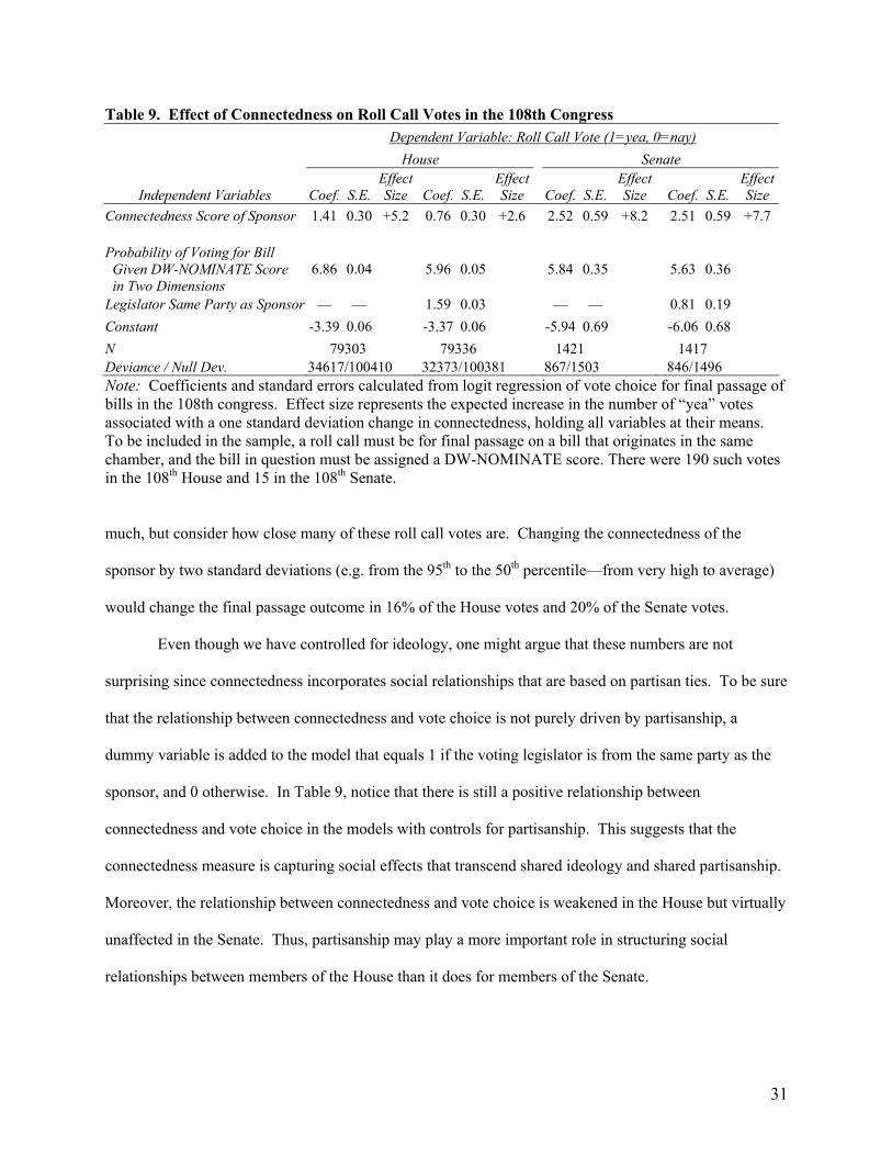
31

Table 9. Effect of Connectedness on Roll Call Votes in the 108th Congress Dependent Variable: Roll Call Vote (1=yea, 0=nay) House Senate

Independent Variables Coef. S.E.Effect Size Coef. S.E.

Effect Size Coef. S.E.

Effect Size Coef. S.E.

Effect Size

Connectedness Score of Sponsor 1.41 0.30 +5.2 0.76 0.30 +2.6 2.52 0.59 +8.2 2.51 0.59 +7.7 Probability of Voting for Bill Given DW-NOMINATE Score in Two Dimensions

6.86

0.04

5.96

0.05

5.84

0.35

5.63

0.36

Legislator Same Party as Sponsor — — 1.59 0.03 — — 0.81 0.19 Constant -3.39 0.06 -3.37 0.06 -5.94 0.69 -6.06 0.68 N 79303 79336 1421 1417 Deviance / Null Dev. 34617/100410 32373/100381 867/1503 846/1496 Note: Coefficients and standard errors calculated from logit regression of vote choice for final passage of bills in the 108th congress. Effect size represents the expected increase in the number of “yea” votes associated with a one standard deviation change in connectedness, holding all variables at their means. To be included in the sample, a roll call must be for final passage on a bill that originates in the same chamber, and the bill in question must be assigned a DW-NOMINATE score. There were 190 such votes in the 108th House and 15 in the 108th Senate.

much, but consider how close many of these roll call votes are. Changing the connectedness of the

sponsor by two standard deviations (e.g. from the 95th to the 50th percentile—from very high to average)

would change the final passage outcome in 16% of the House votes and 20% of the Senate votes.

Even though we have controlled for ideology, one might argue that these numbers are not

surprising since connectedness incorporates social relationships that are based on partisan ties. To be sure

that the relationship between connectedness and vote choice is not purely driven by partisanship, a

dummy variable is added to the model that equals 1 if the voting legislator is from the same party as the

sponsor, and 0 otherwise. In Table 9, notice that there is still a positive relationship between

connectedness and vote choice in the models with controls for partisanship. This suggests that the

connectedness measure is capturing social effects that transcend shared ideology and shared partisanship.

Moreover, the relationship between connectedness and vote choice is weakened in the House but virtually

unaffected in the Senate. Thus, partisanship may play a more important role in structuring social

relationships between members of the House than it does for members of the Senate.

32

Conclusion

In this article I use legislative cosponsorship networks to pose several possible answers to the

question “who is the best-connected legislator in the U.S. Congress?” Analysis of these networks reveals

several interesting features. Institutional changes in the rules regarding cosponsorship seem to have had

only a minor effect—for example, legislators in the House submitted duplicate bills to accommodate

additional signatures when there was a 25 cosponsor maximum. An analysis of the distance (geodesic)

between legislators shows that the House and Senate are both densely connected, but the Senate is even

more densely connected than the House, conforming to recent work on the committee assignment

network (Porter et al. 2005). Moreover, there appears to be a great deal of mutual cosponsorship in the

network. Legislators who receive support tend to return the favor.

I use several traditional measures of centrality to estimate the prominence of each legislator in the

network and then report the top scoring individuals in several categories. These methods identify several

plausible candidates for the title “best-connected legislator,” but they do not take advantage of

information about the number of bills cosponsored and the number of cosponsors per bill to estimate the

strength of each tie. I include this information in a measure of legislative ‘connectedness’. Applying the

connectedness measure to all the legislators in the network, I find that the strongest ties between

legislators occur between committee chairs and ranking members (institutional ties), legislators from the

same state or contiguous districts (regional ties), legislators who work closely together on a particular

issue (issue-based ties), and those who are friends (personal ties). Legislators with high connectedness

scores tend to sponsor more legislation and acquire more cosponsors, but some manage to score highly by

being connected to other legislators who are themselves well-connected.

Scholars with detailed knowledge of the legislators studied here may have different opinions

about whether or not those with high connectedness scores are actually “well-connected.” However,

connectedness appears to outperform other measures of centrality in predicting the number of successful

amendments proposed by each legislator. This result is important because past work has used

amendments passed as a proxy for legislative influence. The connectedness measure also helps to predict

33

legislator roll call votes, even when controlling for ideology and party affiliation. Legislators are more

likely to vote for final passage of bills sponsored by well-connected Senators and Representatives. Since

many roll call votes are closely contested, even small changes in the connectedness of the sponsor can

change a significant fraction of the legislative outcomes.

The connectedness measure thus helps to identify the most influential legislators. We might

alternatively use expert evaluations to identify the most influential legislators, but doing so for several

Congresses would be costly, time-consuming, and subject to the partisan bias of the evaluators. In

contrast, connectedness scores are calculated using publicly available data and an objective, automatic

process that requires very little manpower. Moreover, the cosponsorship data used by this process is

based directly on the actions of legislators instead of third-party opinions about those actions, increasing

the chance that the measure is based on decisions that are actually relevant to the legislators under study.

Opportunities for future empirical work abound. For example, this work raises several questions

about the correlates of connectedness. Are better connected legislators more senior? Do better connected

legislators come from the Republicans or the Democrats? The majority party or the minority party?

Liberals, moderates, or conservatives? What is the relationship between district characteristics and

connectedness? Are richer or better educated districts more likely to have well-connected legislators?

Does district ideology or partisanship play a role? This work also raises several questions related to

legislative effectiveness and electoral success. What impact do previous connectedness scores have on

within-party leadership prospects and future committee portfolios? What is the relationship between

connectedness and election results? Are quality challengers less likely to enter contests against well-

connected incumbents? Are well-connected legislators more effective at soliciting campaign

contributions? Do previous elections affect future connectedness? The answers to these questions should

help us to understand better the important role that social networks and personal relationship play in the

exercise of political power.

34

References Beck, P. A., R. J. Dalton, S. Greene, and R. Huckfeldt. 2002. "The Social Calculus of Voting:

Interpersonal, Media, and Organizational Influences on Presidential Choices." American Political Science Review 96 (1):57-73.

Bernard, H. R., P. D. Killworth, M. J. Evans, C. McCarty, and G. A. Shelley. 1988. "Studying Social Relations Cross-Culturally." Ethnology 2 (155-179).

Bonacich, P. 1972. "Factoring and Weighing Approaches to Clique Identification." Journal of Mathematical Sociology 2:113-120.

Burkett, Tracy. 1997. Cosponsorship in the United States Senate: A Network Analysis of Senate Communication and Leadership, 1973-1990. PhD Dissertation, Sociology, University of South Carolina, Columbia.

Caldeira, Gregory A., John A. Clark, and Samuel C. Patterson. 1993. "Political Respect in the Legislature." Legislative Studies Quarterly 18 (3):3-28.

Campbell, James E. 1982. "Cosponsoring Legislation in the U.S. Congress." Legislative Studies Quarterly 7 (3):415-422.

Cormen, T. H., C. E. Leiserson, R. L. Rivest, and C. Stein. 2001. Introduction to Algorithms. 2nd ed. Cambridge, MA: MIT Press.

de Nooy, Wouter, Andrej Mrvar, and Vladimir Batagelj. 2005. Exploratory Social Network Analysis with Pajek, Structural Analysis in the Social Sciences. New York: Cambridge University Press.

Ebel, H., L.-I. Mielsch, and S. Bornholdt. 2002. "Scale-Free Topology of E-Mail Networks." Physical Review E 66 (035103).

Fararo, T. J., and M. Sunshine. 1964. A Study of a Biased Friendship Network. Syracuse: Syracuse University Press.

Faust, Katherine, and John Skvoretz. 2002. "Comparing Networks across Space and Time, Size and Species." Sociological Methodology 32:267-299.

Fowler, James H. 2005. "Turnout in a Small World". In The Social Logic of Politics, edited by A. Zuckerman. Philadelphia: Temple University.

Freeman, L. C. 1977. "Set of Measures of Centrality Based on Betweenness." Sociometry 40 (1):35-41. Freeman, LC, SP Borgatti, and DR White. 1991. "Centrality in Valued Graphs - a Measure of

Betweenness Based on Network Flow." Social Networks 13 (2):141-154. Galaskiewicz, J., and P. V. Marsden. 1978. "Interorganizational Resource Networks: Formal Patterns of

Overlap." Social Science Research 7:89-107. Hall, Richard L. 1992. "Measuring Legislative Influence." Legislative Studies Quarterly 17 (2):205-231. Highton, B. 2000. "Residential Mobility, Community Mobility, and Electoral Participation." Political

Behavior 22 (2):109-120. Hindman, Matthew, Kostas Tsioutsiouliklisz, and Judy A. Johnson. 2003. Googlearchy: How a Few

Heavily-Linked Sites Dominate Politics on the Web. Cambridge, MA. Huckfeldt, R., P. A. Beck, R. J. Dalton, and J. Levine. 1995. "Political Environments, Cohesive Social-

Groups, and the Communication of Public-Opinion." American Journal of Political Science 39 (4):1025-1054.

Kessler, Daniel , and Keih Krehbiel. 1996. "Dynamics of Cosponsorship." The American Political Science Review 90 (3):555-566.

Koger, Gregory. 2003. "Position Taking and Cosponsorship in the U.S. House." Legislative Studies Quarterly 28 (2):225-246.

Krehbiel, Keith. 1995. "Cosponsors and Wafflers from a to Z." The American Journal of Political Science 39 (4):906-923.

Mariolis, P. 1975. "Interlocking Directorates and Control of Corporations: The Theory of Bank Control." Social Science Quarterly 56:425-439.

Mayhew, David R. 1974. Congress: The Electoral Connection, Yale Studies in Political Science ; 26. New Haven: Yale University Press.

35

McGrory, Mary. 1995. Mccain, Gramm a Strange Pairing. Omaha World Herald, November 18, 1995, 17.

Moody, J. 2001. "Race, School Integration, and Friendship Segregation in America." American Journal of Sociology 107:679-716.

Newman, Mark E. J. 2001a. "Scientific Collaboration Networks: I. Network Construction and Fundamental Results." Physical Review E 64 (016131).

Newman, Mark E. J. 2001b. "Scientific Collaboration Networks: Ii. Shortest Paths, Weighted Networks, and Centrality." Physical Review E 64 (016132).

Panning, William H. 1982. "Blockmodels: From Relations to Configurations." American Journal of Political Science 26 (3):585-608.

Pellegrini, PA, and JT Grant. 1999. "Policy Coalitions in the Us Congress: A Spatial Duration Modeling Approach." Geographical Analysis 31 (1):45-66.

Polsby, Nelson W., and Eric Schickler. 2002. "Landmarks in the Study of Congress since 1945." Annual Review of Political Science 5:333-367.

Poole, K. T., and H. Rosenthal. 1985. "A Spatial Model for Legislative Roll Call Analysis." American Journal of Political Science 29 (2):357-384.

Poole, Keith T., and Howard Rosenthal. 1997. Congress: A Political-Economic History of Roll Call Voting. New York: Oxford University Press.

Porter, Mason A., Peter J. Mucha, M. E. J. Newman, and Casey M. Warmbrand. 2005. "A Network Analysis of Committees in the U.S. House of Representatives." Proceedings of the National Academy of Sciences of the United States of America 102:7057-7062.

Proctor, C. H., and C. P. Loomis. 1951. Analysis of Sociometric Data. In Research Methods in Social Relations, edited by P. W. Holland and S. Leinhardt. New York: Dryden Press.

Rapoport, A., and W. J. Horvath. 1961. "A Study of a Large Sociogram." Behavioral Science 6:279-291. Rothenberg, RB, JJ Potterat, and DE Woodhouse. 1995. "Choosing a Centrality Measure - Epidemiologic

Correlates in the Colorado-Springs Study of Social Networks." Social Networks 17 (3-4):273-297.

Sabidussi, G. 1966. "The Centrality Index of a Graph." Psychometrika 31:581-603. Schiller, Wendy J. 1995. "Senators and Political Entrepreneurs: Using Bill Sponsorship to Shape

Legislative Agendas." The American Journal of Political Science 39 (1):186-203. Sinclair, Barbara. 1989. The Transformation of the U.S. Senate. Baltimore, MD: Johns Hopkins

University. Smith, Steven. 1989. Call to Order. Washington, DC: Brookings Institution. Straits, B. C. 1990. "The Social-Context of Voter Turnout." Public Opinion Quarterly 54 (1):64-73. Talbert, JC, and M Potoski. 2002. "Setting the Legislative Agenda: The Dimensional Structure of Bill

Cosponsoring and Floor Voting." Journal of Politics 64 (3):864-891. Weingast, Barry. 1991. Fighting Fire with Fire: Amending Activity and Institutional Change in the

Postreform Congress. In The Postreform Congress, edited by R. Davidson. New York.: St. Martin’s Press.

Wilson, Rick K., and Cheryl D. Young. 1997. "Cosponsorship in the United States Congress." Legislative Studies Quarterly 22 (1):24-43.