December, 2017

Working Paper No. 17-041

Who Becomes an Inventor in America? The Importance of Exposure to Innovation

Alex Bell Harvard University

Xavier Jaravel

London School of Economics

John Van Reenen MIT and Center for Economic

Performance

Raj Chetty Stanford University and NBER

Neviana Petkova

Office of Tax Analysis, US Treasury

Who Becomes an Inventor in America?The Importance of Exposure to Innovation∗

Alex Bell, Harvard UniversityRaj Chetty, Stanford University and NBERXavier Jaravel, London School of Economics

Neviana Petkova, Office of Tax Analysis, US TreasuryJohn Van Reenen, MIT and Centre for Economic Performance

December 2017

Abstract

We characterize the factors that determine who becomes an inventor in America by using de-identified data on 1.2 million inventors from patent records linked to tax records. We establishthree sets of results. First, children from high-income (top 1%) families are ten times as likelyto become inventors as those from below-median income families. There are similarly large gapsby race and gender. Differences in innate ability, as measured by test scores in early child-hood, explain relatively little of these gaps. Second, exposure to innovation during childhoodhas significant causal effects on children’s propensities to become inventors. Growing up in aneighborhood or family with a high innovation rate in a specific technology class leads to ahigher probability of patenting in exactly the same technology class. These exposure effects aregender-specific: girls are more likely to become inventors in a particular technology class if theygrow up in an area with more female inventors in that technology class. Third, the financialreturns to inventions are extremely skewed and highly correlated with their scientific impact,as measured by citations. Consistent with the importance of exposure effects and contrary tostandard models of career selection, women and disadvantaged youth are as under-representedamong high-impact inventors as they are among inventors as a whole. We develop a simple modelof inventors’ careers that matches these empirical results. The model implies that increasingexposure to innovation in childhood may have larger impacts on innovation than increasing thefinancial incentives to innovate, for instance by reducing tax rates. In particular, there are many“lost Einsteins” – individuals who would have had highly impactful inventions had they beenexposed to innovation.

∗A preliminary draft of this paper was previously circulated under the title “The Lifecycle of Inventors.” Theopinions expressed in this paper are those of the authors alone and do not necessarily reflect the views of the InternalRevenue Service, U.S. Department of the Treasury, or the National Institutes of Health. We would particularly liketo thank Philippe Aghion, with whom we started thinking about these issues, for inspiration and many insightfulcomments. We would like to also thank Daron Acemoglu, Ufuk Akcigit, Olivier Blanchard, Erik Hurst, DannyKahnemann, Pete Klenow, Henrik Kleven, Richard Layard, Eddie Lazear, Josh Lerner, Alex Olssen, Jim Poterba,Scott Stern, Otto Toivanen, Heidi Williams and numerous seminar participants for helpful comments and discussions.Trevor Bakker, Augustin Bergeron, Mike Droste, Jamie Fogel, Nikolaus Hidenbrand, Alexandre Jenni, BenjaminScuderi, and other members of the Equality of Opportunity Project research team provided outstanding researchassistance. This research was funded by the National Science Foundation, the National Institute on Aging GrantT32AG000186, the Lab for Economic Applications and Policy at Harvard, the European Research Council, theEconomic and Social Research Council at CEP, the Kauffman Foundation, the Bill and Melinda Gates Foundation,and the Robert Wood Johnson Foundation.

I Introduction

Innovation is widely viewed as a central driver of economic growth (e.g., Romer 1990, Aghion and

Howitt 1992). As a result, many countries use a variety of policies to spur innovation, ranging from

tax incentives to technical education. One way to understand the effectiveness of such policies is

to study the determinants of who becomes an inventor. What types of people become success-

ful inventors today? What do their experiences teach us about the factors that affect rates of

innovation?

Relatively little is known about the characteristics of inventors because most sources of data

on innovation (e.g., patent records) do not record even basic demographic information, such as an

inventor’s age or gender. In this paper, we present the first comprehensive portrait of inventors in

the United States. Following standard practice in prior work on innovation, we define an “inventor”

as an individual who holds a patent.1 We link data on the universe of patent applications and

grants in the U.S. between 1996 and 2014 to federal income tax returns to construct a panel

dataset covering 1.2 million inventors (patent applicants or recipients). Using this new dataset, we

track inventors’ lives chronologically from birth to adulthood to identify factors that determine who

becomes an inventor and the types of policies that may be most effective in increasing innovation.

In the first part of our empirical analysis, we show that children’s characteristics at birth –

their socioeconomic class, race, and gender – are highly predictive of their propensity to become

inventors. Children born to parents in the top 1% of the income distribution are ten times as likely

to become inventors as those born to families with below-median income.2 Whites are more than

three times as likely to become inventors as blacks. And 82% of 40-year-old inventors today are

men. This gender gap in innovation is shrinking gradually over time, but at the current rate of

convergence, it will take another 118 years to reach gender parity. Putting these data together, we

estimate that if women, minorities, and children from lower-income families were to invent at the

same rate as white men from high-income (top-quintile) families, the total number of inventors in

the economy would quadruple.

1The use of patents as a proxy for innovation has well-known limitations (e.g. Griliches 1990, OECD 2009).In particular, not all innovations are patented and not all patents are meaningful innovations. We address thesemeasurement issues by showing that (a) our results hold if we focus on highly-cited (i.e., high-impact) patents and(b) the mechanisms that lead to the differences in rates of patenting across subgroups that we document are unlikelyto be affected by these concerns.

2This pattern is not unique to innovation: children from high-income families are also substantially more likely toenter other high-skilled professional occupations and, more generally, reach the upper-tail of the income distribution.We focus on innovation here because it is thought to have particularly large social spillovers and because focusing oninnovation has methodological advantages in understanding the mechanisms underlying career choice, as we discussbelow.

1

Why do rates of innovation vary so sharply based on characteristics at birth? In economic

models, any choice can be traced to three exogenous factors: endowments (e.g., differences in

genetic ability across subgroups), preferences (e.g., a greater taste for pursuing science or a career

with risky returns), or constraints (e.g., a lack of liquidity or opportunities to build human capital).

Since each of these explanations has very different implications for policies that can be used to

increase innovation, we structure most of our analysis around assessing the relative importance of

these three mechanisms.

As a first step, we evaluate whether differences in ability explain these gaps in innovation using

test scores in early childhood as a proxy for ability. We obtain data on test scores from 3rd to

8th grade by linking school district records for 2.5 million children who attended New York City

public schools to the patent and tax records. Math test scores in 3rd grade are highly predictive

of patent rates, but they account for less than one-third of the gap in innovation between children

from high- vs. low-income families.3 This is because children from lower income families are much

less likely to become inventors even conditional on having test scores at the top of their 3rd grade

class. Differences in 3rd grade math scores also explain a small share of the gap in innovation by

race, and virtually none of the gap in innovation by gender.

The gap in innovation explained by test scores grows in later grades, consistent with prior

evidence that test score gaps widen as children progress through school (e.g., Fryer and Levitt 2004,

Fryer 2011). Half of the gap in innovation by parent income can be explained by differences in math

test scores in 8th grade. These results suggest that low-income children start out on relatively even

footing with their higher-income peers in terms of innovation ability, but fall behind over time,

perhaps because of differences in their childhood environment. However, they do not provide

conclusive evidence about the role of environment because test scores are an imperfect measure of

ability. If a child’s ability to innovate is poorly captured by standardized tests, particularly at early

ages, ability could still account for a substantial share of gaps in innovation.4

In the second part of our empirical analysis, we address this issue by studying the impacts of

childhood environment directly. We show that exposure to innovation during childhood through

one’s family or neighborhood has a significant causal effect on a child’s propensity to become an

3Test scores in English have no predictive power conditional on test scores in math, suggesting that tests in earlychildhood are diagnostic of specific skills that matter for innovation.

4On the other hand, since children from different socioeconomic backgrounds are exposed to different environmentseven before they enter school, these calculations could overstate the portion of the gap in innovation that is due todifferences in ability.

2

inventor.5 We establish this result – which we view as the central empirical result of the paper – in

a series of steps. We first show that children who grow up in commuting zones (CZs) with higher

patent rates are significantly more likely to become inventors, even conditional on the CZ in which

they work in adulthood. We then show this pattern holds not just for whether a child innovates

but also in the technology category in which he or she innovates. For example, among people living

in Boston, those who grew up in Silicon Valley are especially likely to patent in computers, while

those who grew up in Minneapolis – which has many medical device manufacturers – are especially

likely to patent in medical devices. We find similar patterns at the family level: children whose

parents or parents’ colleagues hold patents in a technology class are more likely to patent in exactly

that field themselves.

These patterns of transmission hold even across the 445 narrowly defined technology subclasses

into which patents can be classified. For example, a child whose parents hold a patent in amplifiers

is much more likely to patent in amplifiers himself than in antennas. Moreover, the patterns are

gender-specific: women are much more likely to patent in a specific technology class if female workers

in their childhood CZ were especially likely to patent in that class. Conditional on women’s patent

rates, men’s patent rates have no predictive power for women’s innovation. Conversely, men’s

innovation rates are influenced by male rather than female inventors in their area.

Under the assumption that differences in genetic ability do not generate differences in propen-

sities to innovate across narrow technology classes in a gender-specific manner, this set of results

on patenting by technology class implies that exposure to innovation during childhood has a causal

effect on innovation. Intuitively, as long as genetics do not govern one’s ability to invent an ampli-

fier rather than an antenna in a gender-specific manner, the close alignment between the subfield

in which children innovate and the type of innovation they were exposed to in their families or

neighborhoods must be driven by causal exposure effects. Formally, the sharp variation in rates of

innovation across technology classes and gender subgroups provides a set of overidentifying restric-

tions that allow us to distinguish exposure effects from plausible models of selection in observational

data.

We estimate that moving a child from a CZ that is at the 25th percentile of the distribution

in terms of innovation (e.g., New Orleans, LA) to the 75th percentile (e.g., Austin, TX) would

increase his or her probability of becoming an inventor by at least 17% and potentially as much

5We use the term “exposure to innovation” to mean having contact with someone in the innovation sector, e.g.through one’s family or neighbors. We do not distinguish between the mechanisms through which such exposurematters, which could range from specific human capital accumulation to changes in aspirations.

3

as 50%. These exposure effects are consistent with recent evidence documenting neighborhood

exposure effects on earnings, college attendance, and other outcomes (Chetty et al. 2016, Chetty

and Hendren 2017). Neighborhood effects have typically been attributed to factors that affect

general human capital accumulation, such as the quality of local schools or residential segregation.

Our findings show that, at least in the context of innovation, such mechanisms are unlikely to be

the sole reason that childhood environment matters, as it is implausible that some neighborhoods

prepare children to innovate in one particular technology class such as amplifiers. Rather, they

point to mechanisms such as transmission of specific human capital, mentoring, or networks (e.g.,

through internships) that lead children to pursue certain career paths. Children from low-income

families, minorities, and women are less likely to have such exposure through their families and

neighborhoods, which helps explain why they have significantly lower rates of innovation overall.

For example, our estimates imply that if girls were as exposed to female inventors as boys are to

male inventors in their childhood CZs, the gender gap in innovation would be half as large as it

currently is.

Stepping forward chronologically in studying children’s environments, we next examine how

rates of innovation vary across colleges. Students from low-income and high-income families at the

colleges with the most inventors (e.g., MIT) go on to patent at relatively similar rates, supporting

the view that factors that affect children before they enter the labor market are a key determinant of

who becomes an inventor. For example, liquidity constraints in financing innovation or differences

in risk preferences are unlikely to explain why low-income children innovate at lower rates, as such

explanations would generate differences in rates of innovation even conditional on the college a

child attends.

In the third part of our empirical analysis, we examine inventors’ careers after entering the

labor market, with the aim of understanding how financial incentives affect individuals’ decisions

to become inventors. We find that the financial returns to innovation are highly skewed and

highly correlated with their scientific impact – two key facts which we later show (using a standard

model of career choice) imply that small changes in financial incentives will not affect aggregate

innovation significantly. In particular, the top 1% of inventors obtain more than 22% of total

inventors’ income, implying that the distribution of income among patent-holders is as skewed as

the distribution of income in the population as a whole. Individuals with highly cited patents

have much higher incomes, showing that the private benefits of innovation are correlated with their

4

scientific impacts.6 The highest-impact patents are most commonly obtained when individuals are

in their mid-forties – well after individuals make career choices – consistent with prior work (e.g.,

Jones et al. 2014). Much of this income is earned in the years before patents are granted, implying

that they are not just returns from the patent itself but from associated businesses or salaries.7

Inventors from under-represented groups (women, minorities, and those from low-income fami-

lies) have very similar earnings and citations to other inventors on average. This result challenges

standard models that explain differences in occupational choice by differences in barriers to entry

across subgroups (e.g., Hsieh et al. 2016). Under the assumption that the ability to innovate does not

vary across groups, such “rational sorting” models predict that the individuals from disadvantaged

groups who become inventors will have higher productivity than inventors from more advantaged

backgrounds, since the marginal inventors who are screened out are those with lower potential. In

fact, we find the opposite: inventors from disadvantaged groups do not have higher-impact inno-

vations on average. Put differently, women and disadvantaged youth are just as under-represented

among star inventors as they are among inventors as a whole. This finding is consistent with the

view that exposure is a central determinant of innovation. In particular, a lack of exposure may

prevent some individuals from pursuing a career in innovation even though they would have had

highly impactful innovations had they done so (“lost Einsteins,” as in Celik (2014)).8

We characterize the implications of our empirical findings for policies to increase innovation us-

ing a simple model of career choice in which three factors determine whether an individual pursues

innovation: financial incentives (Roy 1951), barriers to entry (Hsieh et al. 2016), and exposure to

innovation, which is the new element we introduce given our empirical results. We model exposure

as a binary variable: individuals who do not receive exposure to innovation never pursue innovation,

while those who receive exposure decide whether to pursue innovation by maximizing expected life-

time utility. Using this model, we contrast three types of policies to increase innovation: increasing

exposure (e.g., through internships), reducing barriers to entry (e.g., by providing subsidies for

certain subgroups), and increasing private financial returns (e.g., by cutting top income tax rates

on inventors).

6We follow prior work (e.g., Jaffe et al. 1993) in using patent citations as a proxy for a patent’s scientific impact.Although citations are an imperfect proxy for impact, they are well correlated with other measures of value, such asfirm’s profits and market valuations (Scherer et al. 2000, Hall et al. 2005, Abrams et al. 2013, Kogan et al. 2017).

7Aghion et al. (2017) and Depalo and Di Addario (2015) document analogous patterns in Finland and Italy. Wefocus exclusively on the impacts of patents on inventors’ own earnings; see Van Reenen (1996) and Kline et al. (2017)for analyses of how innovation affects co-workers wages in the inventor’s firm.

8These results could be explained by a model in which the hurdles that generate barriers to entry (e.g., discrimi-nation) also reduce an individual’s productivity after entering innovation. Regardless of the underlying explanation,however, the under-representation of certain groups among star inventors implies that there are “lost Einsteins.”

5

The model implies that the potential to increase innovation by reducing barriers to entry or

increasing financial returns is limited, for three reasons. First, such policies only affect the subset of

individuals who have exposure. Second, if the returns to innovation are forecastable at the point of

career choice, such policies would only induce inventors of marginal quality to enter the field rather

than star inventors (Jaimovich and Rebelo 2017). The mean annual income of those with patents

in the top 1% of the citation distribution is more than $1 million between ages 40-50. The decisions

of these star inventors are unlikely to be affected by small changes in financial incentives, making

aggregate quality-weighted innovation relatively insensitive to tax rates. Third, if the returns to

innovation are uncertain at the point of career choice, the elasticity of innovation with respect to

top income tax rates is likely to be small in a standard expected utility model because tax changes

only affect payouts when inventors have very high incomes and low marginal utility.

In contrast, the model implies that increasing exposure can have substantial impacts on quality-

weighted innovation by drawing individuals who produce high-impact inventions into the innovation

pipeline. In particular, increasing exposure to innovation specifically among children who (a) excel

in math and science at early ages and (b) are from under-represented groups can have large returns,

since the gaps in innovation rates by parental income, race, and gender are largest among children

who have very high test scores in early grades.

It is important to keep two caveats in mind when interpreting the conclusions we draw from our

model. First, our analysis focuses exclusively on the decisions of individual inventors. Taxes and

financial incentives could potentially affect innovation through many other channels, for instance

by changing the behavior of firms, other salaried workers who contribute to the innovation process,

or through general equilibrium effects (e.g., Lerner and Wulf 2007, Akcigit et al. 2017). Taxes may

also influence inventors’ behavior on other margins, such as how much effort to supply or where to

locate (Akcigit et al. 2016, Moretti and Wilson 2017), which are distinct from the extensive margin

career choice decisions we focus on here. Second, our analysis does not provide guidance on the

impacts of specific policies to increase exposure to innovation. To facilitate future work evaluating

such policies, we construct a set of publicly available data tables that provide statistics on patent

rates and citations by technology category, parent income group, gender, age, commuting zone, and

college. In addition, we report statistics on inventors’ income distributions by year and citations.

These tables can be used to study a variety of issues, ranging from the impacts of local economic

conditions on rates and types of innovation to how the returns to innovation have changed over

time.

6

Related Literature. Our results build on and contribute to several literatures. First, our results

relate to the literature on career choice (e.g., Topel and Ward 1992, Hall 2002). Some studies in

this literature have used data on specific occupations – such as medicine and law – to show that

children are particularly likely to pursue their parents’ occupations (e.g., Laband and Lentz 1983,

Lentz and Laband 1989), but they have not separated causal exposure effects from selection effects

as we do here. While the mechanisms we document may apply to other careers as well, we focus on

innovation because of its importance for economic growth (e.g., Jones and Williams 1999, Bloom

et al. 2013) and because inventors’ earnings exhibit much greater cross-sectional variance than most

other highly skilled professions, leading to differences in the predicted impacts of policies such as

tax changes. In addition, from a methodological perspective, patents have the advantage of being

classified into narrow technological classes, allowing us to identify the causal effects of exposure

and show that exposure matters not just for broad career choices but in a granular, subject-specific

manner.

Second, our results relate to the literature on the misallocation of talent across occupations

(e.g., Murphy et al. 1991, Hsieh et al. 2016). Our analysis does not offer any evidence that talent

is misallocated, but our finding that the allocation of talent to innovation is driven partly by

differences in exposure rather than ability is consistent with the premise of this literature.9 Indeed,

our results raise the possibility that the welfare costs of distortions in the allocation of talent may

be even greater than predicted by models such as Hsieh et al. (2016), since some of the individuals

who fail to pursue innovation due to a lack of exposure are superstars rather than marginal entrants.

More broadly, our findings suggest that improving opportunities for children from low-income or

minority backgrounds (e.g., Heckman 2006, Card and Giulano 2014) could increase not just their

own earnings but also economic growth by improving the allocation of talent.

Third, in the literature on innovation itself, most existing research focuses on the “demand side”

of innovation, such as tax credits for research and development (e.g., Becker 2015). Some authors

have called for greater focus on “supply side” policies that increase the number of inventors instead

(e.g., Goolsbee 1998, Romer 2000). Our study takes a step toward understanding the supply side

of innovation by characterizing the behavior of individual inventors. In doing so, it joins a nascent

body of work studying the origins of inventors that draws primarily upon data from Scandinavian

registries. For example, Aghion et al.’s (2017) recent study of inventors in Finland documents gaps

9More precisely, we study the determinants of the allocation of talent across sectors, but do not present anynormative evidence that welfare would be higher if individuals were to choose different occupations.

7

in innovation by parental background consistent with our results and characterizes the predictive

power of other factors that we do not observe in our data, such as IQ and parental education.10 Our

analysis complements the work of Aghion et al. (2017) and other related studies by (a) identifying

different factors that affect innovation, most importantly the causal effect of exposure and (b)

presenting comprehensive data and publicly available statistics on inventors’ origins and careers in

the United States.

The paper is organized as follows. Section II describes the data. Sections III, IV, and V present

our empirical results on inventors’ characteristics at birth, childhood environments, and career

trajectories, respectively. In Section VI, we present the model of inventors’ career choices and

discuss its implications for policies to increase innovation. Section VII concludes. Data tables on

patent rates by subgroup can be downloaded from the Equality of Opportunity Project website.

II Data

In this section, we describe our data sources, define the samples and key variables we use in our

analysis, and present summary statistics.

II.A Data Sources

Patent Records. We obtain information on patents from two sources. First, we use information on

patent grants from a database hosted by Google, which contains the full text of all patents granted

in the U.S. from 1976 to present. We focus on the 1.7 million patents that were granted between

1996 and 2014 to U.S. residents. Second, we use data on 1.6 million patent applications between

2001 and 2012 provided by Strumsky (2014).11

We define an individual as an inventor if he or she is listed as an inventor on a patent application

between 2001-2012 or grant between 1996-2014; for simplicity, we refer to this outcome as “inventing

by 2014” below. Importantly, we include all individuals listed as inventors, not just those assigned

intellectual property rights. In particular, inventors employed by companies are listed as inventors,

while their company is typically listed as the assignee. In addition to inventors’ names, we also

extract information on inventors’ geographic location (city and state) when they filed the patent

10Other studies include Giuri et al. (2007), Azoulay et al. (2011), Toivanen and Vaananen (2012), Dorner et al.(2014), Jung and Ejermo (2014), Lindquist et al. (2015), and Akcigit et al. (2017). A forerunner of this recent workwas a classic study by Schmookler (1957) of 57 inventors.

11In 2001, the U.S. began publishing patent applications (and not just patent grants) 18 months after filing. Fora fee, applicants can choose to have their filing kept secret; 15% of applicants choose to do so. To ensure that thismissing data problem does not generate selection bias, we verify that the results we report below are all robust todefining inventors purely using patent grants rather than applications.

8

and the 3-digit technology class to which the patent belongs, as assigned by the United States

Patent and Trademark Office (USPTO). We classify patents into technology categories using the

classification developed in the NBER Patent Data Project by Hall et al. (2001). We assign each

inventor in our data a single technology class based on the class in which he or she has the most

patents, breaking ties randomly. We obtain data on the number of times each granted patent was

cited from its issuance date until 2014 from the USPTO’s full-text issuance files.

Tax Records. We use federal income tax records spanning 1996-2012 to obtain information such

as an individual’s gender and age, geographic location, and own and parental income. The tax

records cover all individuals who appear in the Death Master file produced by the Social Security

Administration, which includes all persons in the U.S. with a Social Security Number or Individual

Taxpayer Identification Number (ITIN). The data include both income tax returns (1040 forms)

and third-party information returns (e.g., W-2 forms), which give us information on the earnings

of those who do not file tax returns.

The patent data were linked to the tax data using an inventor’s name, city, and state. In

the tax data, these fields were obtained from the Death Master file, 1040 forms, and third-party

information returns (see Online Appendix A for a complete description of the matching procedure).

88% of individuals who applied for or were granted a patent were successfully linked, with higher

match rates in more recent years since information returns are unavailable prior to 1999.

We evaluate the quality of our matching algorithm by using external data on ages for a subset

of inventors from Jones (2010). The age of the inventor recorded in the Death Master file matches

the age reported in Jones’s dataset in virtually all cases, confirming that our algorithm generates

virtually no false matches. The 12% of inventors who are not matched are individuals with common

names that are difficult to link to unique records (e.g., “John Smith”), individuals with spelling

errors in their names or addresses, or individuals who listed different addresses on their patent

applications and tax forms. The observable characteristics (in the patent data) of unmatched

inventors are very similar to those of those of matched inventors, suggesting that the individuals

we match are representative of inventors in the U.S.

New York City School District Records. We use data from the New York City (NYC) school

district to obtain information on test scores in childhood for the subset of individuals who attended

New York City public schools. These data span the school years 1988-1989 through 2008-2009

and cover roughly 2.5 million children in grades 3-8. Test scores are available for English language

arts and math for students in grades 3-8 in every year from the spring of 1989 to 2009, with the

9

exception of 7th grade English scores in 2002. These data were linked to the tax data by Chetty

et al. (2014a) with an 89% match rate, and we use their linked data directly in our analysis.

After these three databases were linked, the data were de-identified (i.e., individual identifiers

were removed) and the analysis was conducted using the de-identified dataset.

II.B Sample Definitions

We use three different samples in our empirical analysis: full inventors, intergenerational, and New

York City schools.

Full Inventors Sample. Our first analysis sample consists of all inventors (individuals with patent

grants or applications) who were successfully linked to the tax data. There are approximately 1.2

million individuals in this sample. This sample is structured as a panel from 1996 to 2012, with

data in each year on individual’s incomes, patents, and other variables. We use this sample to

analyze inventors’ labor market careers in Section V.

Intergenerational Sample. Much of our empirical analysis compares inventors to non-inventors in

terms of characteristics at birth (Section III) and childhood environment (Section IV). To measure

conditions at birth and childhood location, we must link individuals to their parents. To do so, we

use the sample constructed by Chetty et al. (2014b) to study intergenerational mobility, focusing

on all children in the tax data who (1) were born in the 1980-84 birth cohorts, (2) can be linked to

parents, and (3) were U.S. citizens as of 2013. Chetty et al. (2014b, Appendix A) describe how this

intergenerational sample is constructed starting from the raw tax data; here, we briefly summarize

its key features.

We define a child’s parents as the first tax filers between 1996 and 2012 to claim the child as a

dependent and were between the ages of 15 and 40 when the child was born. Since children begin to

leave the household after age 16, the earliest birth cohort that we can reliably link to parents is the

1980 birth cohort (who are 16 in 1996, when our data begin). Children are assigned parent(s) based

on the first tax return on which they are claimed, regardless of subsequent changes in the parents’

marital status or dependent claiming. Although parents who never file a tax return cannot be linked

to children, we still identify parents for more than 90% of children, as the vast majority of children

are claimed at some point because of the tax benefits of claiming children. We restrict the sample

to children who are citizens in 2013 to exclude individuals who are likely to have immigrated to the

U.S. as adults, for whom we cannot measure parent income. We cannot directly restrict the sample

10

to individuals born in the U.S. because the database only records current citizenship status.12

Since few individuals patent in or before their early twenties, we focus on individuals in the

1980-84 birth cohorts, who are between the ages of 28-32 in 2012, the last year of our data. There

are 16.4 million individuals in our primary intergenerational analysis sample, of whom 34,973 are

inventors. To assess whether our results are biased by focusing on innovation at relatively early

ages (by age 32), we also examine a set of older cohorts using data from Statistics of Income (SOI)

cross-sections, which provide 0.1% stratified random samples of tax returns prior to 1996. The SOI

cross-sections provide identifiers for dependents claimed on tax forms starting in 1987, allowing us

to link parents to children back to the 1971 birth cohort (Chetty et al. 2014b, Appendix A). There

are approximately 11,000 individuals, of whom 131 are inventors, in the 1971-72 birth cohorts in

the SOI sample that we use to study innovation rates up to age 40.

New York City Schools Sample. When analyzing whether test scores explain differences in rates

of innovation (Section III), we focus on the sample of children in the NYC public schools data

linked to the tax data. We also use this sample when analyzing differences in innovation rates by

race and ethnicity, as race and ethnicity are only observed in the school district data. We focus on

children in the 1979-1985 birth cohorts for the test score analysis because the earliest birth cohort

observed in the NYC data is 1979. As in Chetty et al. (2014a), we exclude students who are in

classrooms where more than 25% of students are receiving special education services and students

receiving instruction at home or in a hospital. There are approximately 430,000 children in our

NYC schools analysis sample, of whom 452 are inventors.

II.C Variable Definitions and Summary Statistics

In this subsection, we define the key variables we use in our analysis and present summary statistics.

We measure all monetary variables in 2012 dollars, adjusting for inflation using the consumer price

index (CPI-U).

Income. We use two concepts to measure individuals’ incomes: wage earnings and total income.

Wage earnings are total earnings reported on an individual’s W-2 forms. wage earnings as well as

self-employment income and capital income. Total income is defined for tax filers as Adjusted

Gross Income (as reported on the 1040 tax return) plus tax-exempt interest income and the non-

taxable portion of Social Security and Disability benefits minus the spouse’s W-2 wage earnings

12In addition, we limit the sample to parents with positive income (excluding 1.5% of children) because parentswho file a tax return – as is required to link them to a child – yet have zero income are unlikely to be representative ofindividuals with zero income while those with negative income typically have large capital losses, which are a proxyfor having significant wealth.

11

(for married filers). Total income includes For non-filers, total income is defined as wage earnings.

Individuals who do not file a tax return and who have no W-2 forms are assigned an income of

zero.13 Because the database does not record W-2’s and other information returns prior to 1999, we

cannot reliably measure individual earnings prior to that year, and therefore measure individuals’

incomes only starting in 1999. Income is measured prior to the deduction of individual income

taxes and employee-level payroll taxes.

Parents’ Incomes. Following Chetty et al. (2014b), we measure parent income as total pre-tax

income at the household level. In years where a parent files a tax return, we define family income

as Adjusted Gross Income (as reported on the 1040 tax return) plus tax-exempt interest income

and the non-taxable portion of Social Security and Disability benefits. In years where a parent does

not file a tax return, we define family income as the sum of wage earnings (reported on form W-2),

unemployment benefits (reported on form 1099-G), and gross social security and disability benefits

(reported on form SSA-1099) for both parents.14 In years where parents have no tax return and

no information returns, family income is coded as zero. As in Chetty et al. (2014b), we average

parents’ family income over the five years from 1996 to 2000 to obtain a proxy for parent lifetime

income that is less affected by transitory fluctuations. We use the earliest years in our sample to

best reflect the economic resources of parents while the children in our sample are growing up.

Geographic Location. In each year, individuals are assigned ZIP codes of residence based on

the ZIP code from which they filed their tax return. If an individual does not file in a given year,

we search W-2 forms for a payee ZIP code in that year. Non-filers with no information returns

are assigned missing ZIP codes. We map ZIP codes to counties and CZs using the crosswalks and

methods described in Chetty et al. (2014b, Appendix A). For children whose parents were married

when they were first claimed as dependents, we always track the mother’s location if marital status

changes.

College Attendance. Chetty et al. (2017) construct a roster of attendance at all colleges in the

U.S. from 1999-2013 by combining information from IRS Form 1098-T, an information return filed

by colleges on behalf of each of their students to report tuition payments, with Pell Grant records

from the Department of Education.15 We assign each child in the intergenerational sample to the

13Importantly, these observations are true zeros rather than missing data. Because the database covers all taxrecords, we know that these individuals have no taxable income.

14Since we do not have W-2’s prior to 1999, parent income is coded as 0 prior to 1999 for non-filers. Assigningnon-filing parents 0 income has little impact on our estimates because only 3.1% of parents in the full analysis sampledo not file in each year prior to 1999 and most non-filers have very low W-2 income (Chetty et al. 2014b). Forinstance, in 2000, the median W-2 income among non-filers in our baseline analysis sample was $0.

15All institutions qualifying for federal financial aid under Title IV of the Higher Education Act of 1965 must file

12

college he or she attends (if any) for the most years between ages 19-22. See Chetty et al. (2017,

Appendix B) for further details on how colleges are identified.

Test Scores. We obtain data on standardized test scores directly from the New York City school

district database. The tests were administered at the New York City school district level during

the period we study. Following Chetty et al. (2014a), we normalize the official scale scores from

each exam (math and English) to have mean zero and standard deviation one by year and grade

to account for changes in the tests across school years.

Summary Statistics. Table I presents descriptive statistics for the three analysis samples de-

scribed above. Column 1 presents statistics for the full inventors sample; columns 2 and 3 consider

inventors and non-inventors in the intergenerational sample; and columns 4 and 5 consider inventors

and non-inventors in the NYC schools sample.

In the full inventors sample, the median number of patent applications between 1996-2012 is 1

and the median number of citations per inventor is also only 1. But these distributions are very

skewed: the standard deviations of the number of patent applications and citations are 11.1 and

118.1, respectively. Inventors have median annual wage earnings of $83,000 and total income of

$100,000. Again, these distributions are very skewed, with large standard deviations and mean

incomes well above the medians. The mean age of inventors is 44 and 13% of inventors in the

sample are women.

The intergenerational and NYC school samples have younger individuals because they are re-

stricted to more recent birth cohorts. As a result, inventors in these subsamples have lower median

incomes, patent applications, and citations than in the full sample.

III Inventors’ Characteristics at Birth

In this section, we study how rates of innovation differ along three key dimensions determined at

birth: parental income, race, and gender. We first document gaps in rates of innovation and then

use test score data to assess the extent to which these gaps can be explained by differences in

ability.

a 1098-T form in each calendar year for any student that pays tuition. The Pell Grant records are used to identifystudents who pay no tuition.

13

III.A Gaps in Innovation by Characteristics at Birth

Parental Income. Figure Ia plots the fraction of children who invent by 2014 vs. their parents’ in-

come percentile using our intergenerational analysis sample (children in the 1980-84 birth cohorts).

We assign parents percentile ranks by ranking them based on their mean household income from

1996 to 2000 relative to other parents with children in the same birth cohort. Children from higher-

income families are significantly more likely to become inventors. 8 out of 1,000 children born to

parents in the top 1% of the income distribution become inventors, 10 times higher than the rate

among those with below-median-income parents. The relationship is steeply upward sloping even

among high-income families: rates of innovation rise by 22% between the 95th and 99th percentile

of the parental income distribution. This pattern suggests that liquidity constraints or differences

in resources are unlikely to fully explain why parent income matters, as liquidity constraints are less

likely to bind at higher income levels and resources presunably have diminishing marginal returns.

Figure Ib shows that the probability a child has highly-cited patents – defined as having total

citations in the top 5% of his or her cohort’s distribution – has a very similar relationship to

parental income. Hence, the relationship between patenting and parent income is not simply

driven by children from high-income families filing low-value or defensive patents at higher rates.

The pattern in Figure I also remains robust at older ages, allaying the concern that children from

higher-income families may simply patent earlier than those from low-income families. In particular,

using the Statistics of Income 0.1% sample, we find that the relationship between rates of innovation

between ages 30 and 40 and parental income remains qualitatively similar (Online Appendix Figure

Ia). Defining inventors purely on the basis of patent grants or patent applications also yields similar

results (Online Appendix Figure Ib).

The relationship between innovation and parental income is representative of the relationship

between achieving professional success and parental income more generally. Children’s propensities

to reach the upper tail of the income distribution have a similarly convex and sharply increasing

relationship with parental income (Online Appendix Figure II). For instance, children with parents

in the top 1% of the parent income distribution are 27 times more likely to reach the top 1% of

their birth cohort’s income distribution and 10.6 times more likely to reach the top 5% of their

cohort’s income distribution than those born to parents below the median. As discussed in the

introduction, we focus on innovation here (rather than professional success in general) because of

innovation’s relevance for economic growth, its unique risk profile, and its advantages in charac-

14

terizing mechanisms more precisely. However, the results and mechanisms we establish here may

apply to other careers beyond innovation.

Race and Ethnicity. Next, we turn to gaps in innovation by race and ethnicity. Since we do

not observe race or ethnicity in the tax data, we use the New York City school district sample

for this analysis. The first set of bars in Figure II shows the fraction of children who patent by

2014 among white non-Hispanic, Black non-Hispanic, Hispanic, and Asian children. 1.6 per 1,000

white children and 3.3 per 1,000 Asian children who attend NYC public schools between grades

3-8 become inventors. These rates are considerably higher than those of Black children (0.5) and

Hispanics (0.2), consistent with evidence from Cook and Kongcharoen (2010).16

Since there are significant differences in parental income by race and ethnicity, the raw gaps

across race and ethnicity partly reflect the income gradient shown in Figure I. To separate these

two margins, we control for differences in income by non-parametrically reweighting the parental

income distributions of Blacks, Hispanics, and Asians to match that of whites in the NYC sample,

following the methodology of DiNardo et al. (1996). We divide the parental income distribution

of children in the NYC sample into ventiles (20 bins) and compute mean patent rates across the

20 bins for each racial/ethnic group, weighting each bin by the fraction of white children whose

parents fall in that income bin (i.e., integrating over the income distribution for whites).

The second set of bars in Figure II plot the resulting innovation rates, which can be interpreted

as the innovation rates that would prevail for each group if it had the same income distribution as

whites. Adjusting for income differences does not eliminate the racial and ethnic gaps, but changes

their magnitudes. The Black-white gap falls by a factor of 2 (from 1.1/1000 to 0.6/1000). The

white-Asian gap widens from 1.7/1000 to 2.6/1000 when we reweight by income, as Asian parents

in NYC public schools have lower incomes on average than white parents. The Hispanic-white gap

remains essentially unchanged.

Gender. Finally, we examine gaps in innovation by gender. Since gender is recorded in the tax

data for all individuals in the population, we use the full inventors sample for this analysis. The

advantage of doing so is that we can examine gender differences in rates of innovation not just for

those born in the 1980s as in our intergenerational sample, but for older cohorts as well.

16The innovation rates are lower than those in Figure Ia because NYC public schools have predominantly low-income students, with more than 75% of students from families with incomes below the national median. NYC publicschools also have a much larger share of minorities than the U.S. population: 19.5% of the children in our NYCsample are white, 9.6% are Asian, 33.7% are Hispanic, and 36.0% are Black. Although we cannot be sure that theracial patterns within the NYC schools hold nationally, we do find that the relationship between parental incomeand innovation in the NYC sample is very similar to the national pattern in Figure Ia, suggesting that it providesrepresentative evidence at least on the socioeconomic dimension (Online Appendix Figure Ic).

15

Figure III plots the fraction of female inventors – individuals who applied for or were granted

a patent between 1996 and 2014 – by birth cohort.17 Consistent with prior work (Thursby and

Thursby 2005, Ding et al. 2006, Hunt 2009, Kahn and Ginther 2017), we find substantial gender

differences in innovation for those in the prime of their careers today; for instance, 18% of inventors

born in 1980 are female. What is less well known from prior work is the rate at which this gap

is changing over time. Figure III shows that the fraction of female inventors was only 7% in the

1940 cohort and has risen monotonically and linearly over time. However, the rate of convergence

is slow: a 0.27 percentage point (pp) increase in the fraction of female inventors per cohort on

average, based on a linear regression. At this rate, it will take another 118 years to reach gender

parity in innovation.

Putting these data together, we estimate that white men from high-income (top-quintile) fam-

ilies are 4.06 times as likely to patent as the average person in the population.18 Hence, if women,

minorities, and children from low-income families were to invent at the same rate as white men

from high-income families, the rate of innovation in the economy would quadruple.

III.B Do Differences in Ability Explain the Gaps in Innovation?

Why do rates of innovation vary so widely across individuals with different characteristics at birth?

In economic models, any choice can be traced to three exogenous factors: endowments (e.g., differ-

ences in ability), preferences (e.g., tastes for risk), or constraints (e.g., a lack of liquidity). In this

subsection, we take a step toward evaluating the first of these factors – innate ability – by using

data on childhood test scores for children in our New York City schools sample. Although students

who attend New York City public schools are a selected subgroup, differences in innovation rates

by parental income (Online Appendix Figure Ic) and gender (Table I) are very similar in the NYC

school district sample as in the full intergenerational sample. We consider whether test scores

explain the gap in innovation within the NYC sample by income, race, and gender in turn.

Parental Income. In Table IIa, we estimate the fraction of the gap in innovation by parental

income that can be explained by math test scores in 3rd grade (the first grade we observe in the

17Because we examine patenting in a fixed time window, we measure patent rates at different ages for differentcohorts, ranging from ages 56-72 for the 1940 cohort to ages 16-32 for the 1980 cohort. This approach yields consistentestimates of the gender gap across cohorts if gender differences in patenting do not vary by age. While we cannotevaluate the validity of this assumption across all cohorts, examining patent rates at a fixed age (e.g., age 40) overthe 17 cohorts we can analyze yields similar results (not reported).

18We do not observe race at the national level, but Census data show that the minority share of families in thetop fifth of the income distribution is less than 5%. The patent rate of white men from high-income families istherefore well approximated by the patent rate of all men from high-income families, which we compute directly inour intergenerational sample.

16

NYC data).19 We define “high-income” children as children with parents in the top income quintile

within the NYC sample, placing all others in the “lower-income” category; using other thresholds

to divide the two groups yields similar results. We focus on math test scores because scores in

English do not predict innovation rates conditional on math scores (Online Appendix Table I).20

The first row of Table II shows that 1.93 out of 1,000 children from top-quintile families born

between 1979-85 invent by 2014, as compared with 0.52 out of 1,000 children from lower-income

families. The raw gap in innovation across these income groups is thus 1.41 inventors per 1,000

children. In the second row, we reweight the test scores of the lower-income students to match

those of children from high income families, following the methodology of DiNardo et al. (1996) as

in our analysis of income and race above. We divide the 3rd grade math test score distribution of

children in the NYC sample into ventiles (20 bins) and compute mean patent rates across the 20

bins for the lower-income group, weighting each bin by the fraction of high-income children with

test scores in that bin. The second row of Table II shows that children from lower-income families

would have a patent rate of 0.96 per 1,000 (rather than 0.52) if they had the same test scores

as children from high-income families. The patent rate rises because children from high-income

families have higher test scores in 3rd grade; for instance, children from the top income quintile

score 0.65 SD higher on average than children from lower quintiles (Online Appendix Figure IIIa).

However, these differences in test scores explain less than 1/3 of the raw gap in innovation, as the

gap remains at 0.97 per 1,000 even after adjusting for differences in test scores, as shown in column

3 of Table II.

Figure IVa illustrates why test scores fail to fully explain the gap in innovation by plotting

innovation rates vs. test scores for children with parents in the top quintile (circles) and those

with lower-income parents (triangles). Each point in this figure shows the fraction of inventors

within a ventile of the test score distribution. In high-income families, children who score highly on

3rd grade math tests are much more likely to become inventors than those with lower test scores.

By contrast, in lower-income families, children with higher test scores do not have much higher

innovation rates. As a result, among students with test scores in the top 5% of the distribution,

those from high-income families are more than twice as likely to become inventors as those from

19Of course, 3rd grade test scores are not a pure measure of intrinsic ability, as children from different socioeconomicbackgrounds are exposed to different environments even before 3rd grade. Nevertheless, we show that 3rd grade testscores can provide informative bounds on the extent to which innovation gaps are driven by ability, particularly whencompared with test scores in later grades.

20The same is not true for success on other dimensions: for instance, both math and English scores are predictiveof the probability that a child reaches the top 1% of the income distribution (Online Appendix Table I).

17

lower-income families. This result suggests that becoming an inventor in America relies on two

traits: having high ability (as proxied for by test scores early in childhood) and being born into a

high-income family.

To obtain further insight into the role of ability, we repeat the preceding analysis using test

scores in later grades. Figure V plots the fraction of the raw gap in innovation that is explained by

math test scores in each grade from grades 3-8. As children get older, test scores account for more

of the gap in innovation by parental income. By 8th grade, 48% of the gap can be explained by

differences in test scores, significantly higher than the 31% in 3rd grade. Based on a linear regression

across the six grades in which we observe scores, we estimate that on average an additional 3.2

percentage points of the gap is explained by test scores each year (p < 0.01).21

Extrapolating linearly back to birth, our estimates imply that only 5.7% of the gap in innovation

would be explained by test scores (ability) at birth. Conversely, test scores at the end of high school

would explain 60.1% of the gap. These results suggest that low-income children start out on even

footing with their higher-income peers in terms of ability, but fall steadily behind as they progress

through school. Indeed, we show below that conditional on the college that children attend, the

gap is innovation by parent income is one-tenth as large as the raw gap shown in Figure I.

Race and Ethnicity. We use an analogous reweighting approach to estimate how much of the

racial gaps in innovation can be accounted for by test scores. The third set of bars in Figure II show

the innovation rates that would prevail if all children had 3rd grade math test scores comparable

to those of whites. The gaps shrink modestly, showing that test scores explain very little of the

racial gaps in innovation. For example, the Black-white gap shrinks from 1.1 to 1.0, a change of

less than 10%, while the Asian-white gap falls by 9%. Figure IVb illustrates why this is the case by

plotting patent rates vs. test scores by race and ethnicity. Even conditional on test scores, whites

and Asians are substantially more likely to become inventors than Blacks and Hispanics. Very few

of even the highest-scoring Black and Hispanic children pursue innovation.

Replicating the reweighting analysis by grade, we find that test scores in later grades explain

more of the racial gaps in innovation, consistent with the patterns for income. For instance, 51%

of the gap in patent rates between Asians and other racial and ethnic groups can be explained by

8th grade test scores.

Gender. Finally, we conduct an analogous exercise for gender, reweighting girls’ test scores

21This result is robust to a variety of alternative specification choices, including using a balanced panel of childrenacross the grades, splitting the sample at the median instead of the 80th percentile of parental income, and controllingfor test scores using regressions instead of reweighting (not reported).

18

to match that of boys. Math test scores in 3rd grade account for only 2.4% of the difference

in innovation rates between males and females (Online Appendix Table II). This is because the

distribution of math test scores for boys and girls is extremely similar in 3rd grade (Online Appendix

Figure IIIb). Similar to the patterns by race and parental income, high-scoring girls are much less

likely to become inventors than high-scoring boys (Figure IVc).

Even in 8th grade, test scores account for only 8.5% of the gender gap in innovation. One

explanation for why the gender gap in test scores expands less across grades than racial and class

gaps is that boys and girls attend similar schools and grow up in similar neighborhoods, whereas

children with different parental income and racial backgrounds do not.

Overall, the results in this section are consistent with evidence from other domains that dis-

parities in ability are small at birth and expand gradually over time (e.g., Fryer and Levitt 2006,

Fryer 2011). One explanation for these patterns is that differences in childhood environment – e.g.,

in the quality of schools or the degree of exposure to science and innovation – affect the amount

students learn or the amount of time they study. However, as noted in prior work, one must be

cautious in attributing these results to environmental differences. If tests at later ages are more

effective at capturing intrinsic ability, one may find the patterns across grades documented above

even in the absence of differences in childhood environment. In light of this limitation, we directly

examine the causal effects of childhood environment in the next section.

IV Childhood Environment and Exposure to Innovation

In this section, we study how differences in a child’s environment prior to entering the labor market

affect rates of innovation. We first characterize the effects of a child’s family and neighborhood,

showing in particular that exposure to innovation has a significant causal effect on a child’s propen-

sity to innovate. We then examine how rates of innovation vary within and across colleges, which

sheds further light on the importance of pre-labor-market factors.

IV.A Parents

To characterize the role that children’s parents play in shaping their decision to pursue innovation,

we begin by asking whether children whose fathers are inventors are more likely to become inventors

themselves.22 In our intergenerational analysis sample (children in the 1980-84 birth cohorts), 2.0

22We focus on fathers here because the vast majority of inventors, particularly in older generations, are male (FigureIII). We examine the role of female inventors in the context of neighborhood differences, where we have greater power,in section IV.B below. We define a father as an inventor if he applied for a patent between 2001-2012 or was granted

19

out of 1,000 children whose parents were not inventors become inventors by 2014. In contrast, 18.0

per 1,000 children of inventors become inventors themselves – a nine-fold difference.23 This pattern

holds even conditional on parental income, across the parent income distribution (not reported).

The intergenerational persistence of innovation could be driven by the genetic transmission of

ability to innovate across generations or by an exposure effect – the environmental effect of growing

up in a family of innovators, holding one’s intrinsic ability fixed. These exposure effects could reflect

the accumulation of specific human capital, changes in preferences, or simply increased awareness

about innovation as a career pathway.

We distinguish between intrinsic ability and exposure effects by exploiting variation in the

specific technology class in which a child innovates. Based on the USPTO’s classification system,

patents can be grouped into seven broad categories (chemicals, computers and communications,

drugs and medical, electrical and electronic, mechanical, design and plant, and other). Within these

categories, patents are further classified into 37 sub-categories and 445 specific technology classes.

These technology classes are very narrow: for instance, within the communications category, there

are separate classes for modulators, demodulators, and oscillators; within the resins subcategory,

there are separate classes for synthetic and natural resins.

We isolate the causal effects of exposure by analyzing whether children are particularly likely to

patent in the same technology classes as their parents. The idea underlying our research design is

that genetic differences in ability are unlikely to lead to differences in propensities to innovate across

similar, narrowly-defined technology classes. For instance, a child is unlikely to have a gene that

codes specifically for ability to invent in modulators rather than oscillators. Under this assumption,

the degree of alignment between the specific technology classes in which children and their parents

innovate can be used to estimate causal exposure effects.

Implementing this research design requires a metric for the degree of similarity between technol-

ogy classes. We define the distance between two technology classes A and B based on the share of

inventors in class A who also invent in class B; the higher the share of common inventors, the lower

the distance between A and B. Online Appendix Table III gives an example that illustrates this

distance metric by showing the technology classes that are closest to technology class 375, “pulse

a patent between 1996-2014, analogous to the definition for children.23Part of this association reflects the fact that children and their fathers sometimes are co-inventors on the same

patent. However, this is relatively rare: 13.7 out of 1,000 children of inventors file patents on which their parentis not a co-inventor, still far higher than the rate for non-inventors. Additionally, our measure of parental inventorstatus suffers from measurement error because we do not observe parents’ patents prior to 1996 in our data, likelyattenuating our estimate of the difference.

20

or digital communications.” Pulse or digital communications has a distance of zero with itself by

definition. Inventors who had a patent in pulse or digital communications were most likely to have

another patent in demodulators, which is therefore assigned an ordinal distance of d = 1 from the

pulse and digital communications class. The next closest class is modulators (d = 2), and so on.

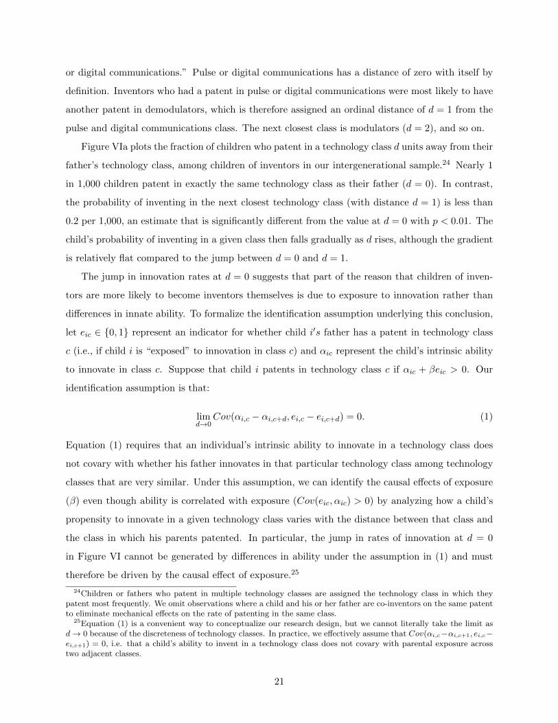
Figure VIa plots the fraction of children who patent in a technology class d units away from their

father’s technology class, among children of inventors in our intergenerational sample.24 Nearly 1

in 1,000 children patent in exactly the same technology class as their father (d = 0). In contrast,

the probability of inventing in the next closest technology class (with distance d = 1) is less than

0.2 per 1,000, an estimate that is significantly different from the value at d = 0 with p < 0.01. The

child’s probability of inventing in a given class then falls gradually as d rises, although the gradient

is relatively flat compared to the jump between d = 0 and d = 1.

The jump in innovation rates at d = 0 suggests that part of the reason that children of inven-

tors are more likely to become inventors themselves is due to exposure to innovation rather than

differences in innate ability. To formalize the identification assumption underlying this conclusion,

let eic ∈ {0, 1} represent an indicator for whether child i′s father has a patent in technology class

c (i.e., if child i is “exposed” to innovation in class c) and αic represent the child’s intrinsic ability

to innovate in class c. Suppose that child i patents in technology class c if αic + βeic > 0. Our

identification assumption is that:

limd→0

Cov(αi,c − αi,c+d, ei,c − ei,c+d) = 0. (1)

Equation (1) requires that an individual’s intrinsic ability to innovate in a technology class does

not covary with whether his father innovates in that particular technology class among technology

classes that are very similar. Under this assumption, we can identify the causal effects of exposure

(β) even though ability is correlated with exposure (Cov(eic, αic) > 0) by analyzing how a child’s

propensity to innovate in a given technology class varies with the distance between that class and

the class in which his parents patented. In particular, the jump in rates of innovation at d = 0

in Figure VI cannot be generated by differences in ability under the assumption in (1) and must

therefore be driven by the causal effect of exposure.25

24Children or fathers who patent in multiple technology classes are assigned the technology class in which theypatent most frequently. We omit observations where a child and his or her father are co-inventors on the same patentto eliminate mechanical effects on the rate of patenting in the same class.

25Equation (1) is a convenient way to conceptualize our research design, but we cannot literally take the limit asd→ 0 because of the discreteness of technology classes. In practice, we effectively assume that Cov(αi,c−αi,c+1, ei,c−ei,c+1) = 0, i.e. that a child’s ability to invent in a technology class does not covary with parental exposure acrosstwo adjacent classes.

21

Interpreting the difference in innovation rates between technology class d = 0 and d = 1 as purely

driven by exposure, we infer that having a parent who is an inventor increases a child’s probability

of being an inventor by at least 0.078 pp through exposure effects.26 Given the mean invention rate

of 0.21 pp in the intergenerational sample, this result implies that exposure to innovation through

one’s parents increases innovation by at least 35%. This calculation is conservative because it

only attributes innovation within the same class to exposure effects. If exposure has more diffuse

impacts across technology classes – as is likely the case – the total impact of exposure to a parental

inventor could be considerably larger. For instance, replicating the analysis in Figure VIa at the

patent sub-category level instead of the class level, we find that children are 0.2 pp more likely to

invent in the same sub-category as their father than the next closest sub-category. If this increase

is entirely due to exposure (i.e., if intrinsic ability to innovate does not vary sharply across similar

sub-categories), then exposure to a parental inventor doubles the probability that a child becomes

an inventor.

In sum, exposure to innovation in one’s family substantially increases the likelihood that a

child pursues innovation.27 Although this result is useful in establishing that exposure matters,

replicating the level of exposure one obtains through one’s parents is likely to be challenging from

a policy perspective. Moreover, parents are only one of many potential sources through which

children may acquire knowledge about careers in innovation. We therefore turn to two broader

sources of exposure outside one’s immediate family: parents’ colleagues and residential neighbors.

IV.B Parents’ Colleagues

In this subsection, we examine how exposure to innovation through parents’ colleagues affects a

child’s propensity to become an inventor. To do so, we first assign each father in our intergenera-

tional sample an industry based on the six-digit NAICS code of his most frequent employer between

1999-2012.28 We then measure the patent rate among workers in the father’s industry – whom we

term the father’s “colleagues” – as the average number of patents issued to individuals in that

26If patent frequencies vary substantially across technology classes, patent rates could vary between the d = 0 andd = 1 groups for mechanical reasons unrelated to exposure, effectively because (1) would be violated by differencesin the size of technology classes. To gauge the extent of such mechanical biases, we verify that there is essentially nochange in patent rates from d = 0 to d = 1 in placebo tests where children were randomly reassigned fathers (notreported).

27This result is consistent with Aghion et al.’s (2017) finding that parental education is highly predictive of achild’s propensity to innovate even conditional on parental income: children with more educated parents may bemore exposed to science and innovation.

28For individuals receiving W-2s from multiple firms in a given year, we define the employer in that year to be thefirm that issued the W-2 with the highest salary. We exclude fathers working in industries with fewer than 50,000individuals (5% of fathers), as patent rates are measured imprecisely for these industries.

22

industry per year (between 1996-2012) divided by the average number of workers in that industry

per year based on counts of W-2 forms in the tax data. To ensure that we do not capture the

effects of parental exposure itself, we drop children whose own parents were inventors throughout

the remainder of this section.

In column 1 of Table III, we regress the fraction of children who become inventors among those

with fathers in a given industry on patent rates for workers in that industry. This regression has

one observation for each of the 345 industries and is weighted by the number of fathers in each

industry.29 The estimate of 0.250 (s.e. = 0.028) implies that a 1 percentage point increase in the

patent rate among a father’s colleagues is associated with a 0.25 percentage point increase in the

probability that a child becomes an inventor. This estimate implies that a one standard deviation

(0.24 pp) increase in the fraction of inventors in the father’s industry is associated with a 25.3%

increase in children’s innovation rates.

The association in column 1 of Table III could reflect either the causal effect of exposure to

innovation through a parents’ colleagues or a correlation with other unobservables, such as a child’s

own intrinsic ability to innovate. As above, we isolate exposure effects by testing whether children

are more likely to innovate in exactly the same technology classes as their parents’ colleagues. Using

the same measure of distance d between technology classes defined in Section IV.A, we estimate

OLS regressions of the form:

ycj = κc + bdPc+d,j + εcj , (2)

where ycj denotes the patent rate in technology class c of children with fathers who work in industry

j, Pc+d,j denotes the patent rate in the class c+ d among workers in industry j, and κc represents

a class-specific intercept. We estimate these regressions at the industry by technology class level,

weighting by the number of children with fathers in each industry. We include class fixed effects

(κc) to account for the variation in size across classes and identify bd from variation across industries

in class-specific patent rates.

Figure VIb plots estimates from regressions analogous to (2). Each bar plots estimates of bd

from a separate regression, varying the distance d used to define workers’ patent rates Pc+d,j in

(2). The first bar plots b0, the relationship between children’s patent rates in a given class and

their fathers’ colleagues patent rates in the same class ( d = 0). In the second bar, we define Pc+d,j

as the mean patent rate in the father’s industry in the next 10 closest classes (d = 1 to 10). The

29This regression is equivalent to regressing an indicator for whether a child is an inventor on the rate of innovationin his or her father’s industry in a dataset with one observation per child, clustering standard errors by industry,because the innovation rate (the right hand side variable) does not vary within industries.

23

third bar uses the average patent rate in classes with d = 11 to 20, and so on. The coefficient bj

on parents’ colleagues’ patent rates drops by 85% from the same class (d = 0) to the next closest

classes (p < 0.01). That is, children are much more likely to patent in exactly the same class as

their parents’ colleagues than in very similar classes. This result implies that an increase in parents’

colleagues patent rates causes an increase in a child’s propensity to innovate under the following

identification assumption:

limd→0

Cov(εc,j − εc+d,j , Pc,j − Pc+d,j) = 0. (3)

This assumption, which is analogous to (1), requires that as the distance d between technology

classes grows small, differences in unobservable determinants of children’s innovation rates in class

c vs. c + d are orthogonal to differences in parents’ colleagues’ innovation rates in those classes.

Intuitively, we require that children whose fathers work in an industry where many workers patent

in amplifiers rather than antennas do not have greater intrinsic ability to invent in amplifiers relative

to antennas themselves. Under this assumption, we can infer from Figure VIb that a 1 pp increase

in patent rates among parental colleagues increases a child’s probability of becoming an inventor

by at least b0 − b1− 10 = 0.065 pp due to a causal exposure effect.

Our measure of distance between technology classes based on co-patenting rates is one of many

potential approaches to identifying “similar” patent classes. To assess the sensitivity of our results

to this choice, we use the USPTO’s hierarchical classification system, which groups patents into

similar fields (categories, sub-categories, and classes), as an alternative way to identify similar patent

classes. In columns 2-5 of Table III, we estimate a series of regressions to assess whether children

patent in the same fields as workers in their father’s industry using the USPTO’s classification

system. In column 2, we test whether children are more likely to invent in the same categories as

their father’s colleagues using a regression specification analogous to (2) estimated at the category

by industry level with d = 0. Columns 3 and 4 replicate the specification in column 2 at the

sub-category and technology class levels. Finally, in column 5 of Table III, we replicate column 4

with three additional controls: patent rates in (i) the same sub-category but in a different patent

class, (ii) the same category but a different sub-category, and (iii) other categories.

At all levels of the hierarchy, we find a strong, statistically significant association between

children’s patent rates and their parents’ colleagues patent rates. Moreover, column 5 shows that

innovation among parents’ colleagues leads to a 10 times larger increase in innovation in exactly

the same technology class (e.g., synthetic resins) as it does in other classes even within the same

24

sub-category (e.g., natural resins). The coefficient on the own-class patent rate is not statistically

different from the specification in column 4, while the coefficients on the other-class and category

patent rates are very close to zero. Under our identification assumption in (3), the much smaller

estimates for other classes imply that children’s propensity to invent in the same class as their

parents’ colleagues is driven by the causal effect of exposure.

The class-specificity of the exposure effects also sheds light on the mechanism through which

exposure matters. Transmission of general human capital or an interest in science would be unlikely

to have impacts that vary so sharply by technology class. Instead, the data point to mechanisms

such as transmission of specific human capital, access to networks that help children pursue a

certain subfield, acquisition of information about certain careers, or role model effects.

IV.C Neighborhoods

In this subsection, we study how rates of innovation in the neighborhood in which a child grows

up affect his or her propensity to innovate. Following Chetty et al. (2014b), we assign children in

our intergenerational sample to commuting zones (CZs) based on where they were first claimed as

dependents by their parents.

Figure VIIa maps rates of innovation across the CZs where children grew up, with darker

colors representing areas where more children become inventors. Figure VIIb lists the ten CZs

where children are the most or least likely to grow up to become inventors (among the 100 most

populated CZs). Children who grow up in the Northeast, coastal California, and the rural Midwest

have the highest probabilities of becoming inventors, while those in the Southeast have the lowest

probability. The areas where children grow up to become inventors tend to have higher mean

incomes (population-weighted correlation ρ = 0.63), fewer single parents (ρ = −0.39), and higher

levels of absolute upward intergenerational mobility (ρ = 0.32), based on the CZ-level measures

defined in Chetty et al. (2014b). However, there are some stark exceptions to these patterns, such

as Detroit, MI, where children have among the highest likelihood of becoming inventors but where

income mobility and mean incomes are relatively low.30

The spatial analysis in Figure VII differs from previous analyses of “innovation clusters” and

agglomeration (e.g., Porter and Stern 2001, Kim and Marschke 2005) because it reflects the locations

where inventors grow up, which may differ from where they work as adults. Nevertheless, children

30We defer a more comprehensive examination of the spatial variation in innovation – which can be conductedusing the CZ-level data that is publicly available in Online Data Table Ia – to future research, focusing here on therole of exposure to innovation during childhood.

25

who grow up in the areas where the most innovation occurs tend to be most likely to go into

innovation themselves. For instance, children who grow up in the San Jose commuting zone, which

includes Silicon Valley, top the list in terms of the probability of becoming inventors themselves.

To examine this relationship more systematically, we define the patent rate of workers in each CZ

as the average number of patents issued per year (in the full USPTO data) to individuals from

a given CZ between 1980 and 1990 divided by the CZ’s population between the ages of 15-64 in

the 1990 Census. Figure VIII presents a scatter plot of the fraction of children who go on to

become inventors vs. the patent rate of workers in their childhood CZ (their “neighbors”) among

the 100 most populated CZs. There is a clear positive relationship between these variables, with a

correlation of 0.75.

The correlation in Figure VIII is consistent with the hypothesis that exposure to innovation

during childhood through one’s neighbors increases a child’s propensity to innovate, but it could

also reflect geographical sorting. We isolate the causal effect of exposure by estimating the extent to

which children invent in the same narrow technology classes as their neighbors, as in our analysis

of industry-level differences above. Figure VIc replicates Figure VIb, plotting coefficients from

regressions of children’s innovation rates in a given technology class c on class-level patent rates

of workers in their childhood CZs vs. the distance between technology classes. The coefficient

on neighbors’ patent rates drops by 85% from the same class (d = 0) to the next closest classes

(p < 0.01). implying that neighborhoods have causal exposure effects under an identification

assumption analogous to (3).

In Table IV, we evaluate the robustness of this result and the mechanisms underlying it using a

set of fixed effects regressions specifications. As a reference, in column 1, we regress the fraction of

children who grow up to be inventors in each CZ on the patent rate of workers in their childhood

CZ, replicating the analysis in Figure VIII including all 741 CZs rather than just the 100 largest

ones. The coefficient of 2.9 implies that a 1 SD (0.02 pp) increase in the annual CZ-level patent rate

is associated with a 0.058 pp (28.5%) increase in the fraction of children who become inventors.

One potential explanation for the result in column 1 (and Figure VIc) is that children tend to

stay near the areas where they grew up, and may mechanically end up being more likely to patent

if they live in an area like Silicon Valley simply because the jobs that are available in such areas

tend to be in the innovation sector. To distinguish this mechanism from childhood exposure effects

that change children’s behavior, we focus on the subset of children who move to a different CZ in

adulthood from where they grew up. In column 2, we estimate a regression analogous to that in

26

column 1 at the childhood CZ by current CZ level, limiting the sample to children whose current

(2012) CZ differs from their childhood CZ. We regress the fraction of children who grow up to be

inventors in each of these cells on the patent rate of the CZ in which they grew up, including fixed

effects for the child’s 2012 CZ so that the coefficient of interest is identified purely from comparisons

across individuals who grew up in different areas but currently live in the same area. The coefficient

on the patent rate in the childhood CZ remains at 2.6 in this specification, showing that most of

the relationship in column 1 is not mechanically driven by the types of jobs available in an area.

In the remaining columns of Table IV, we use the USPTO hierarchical classification system to

identify similar patent classes instead of the distance metric used in Figure VI. In columns 3-5, we

analyze whether the result in Column 1 continues to hold at the category level: do children go on

to patent in the same categories as their neighbors did while they were growing up? We consider

three different specifications. In column 3, we replicate the specification in column 1 at the CZ

by patent category level, using the same specification as in (2) when d = 0, but letting j index

CZs instead of industries. In column 4, we replicate the specification in column 2 at the category

level. We restrict attention to movers and regress the share patenting in a given category (with one

observation per childhood CZ, current CZ, and category) on the childhood CZ patent rate in that

category. We include current CZ fixed by category effects in this specification. In column 5, we

include all children and replace the CZ by category fixed effects with fixed effects for the father’s

industry by category, estimating the model at the childhood CZ by father’s industry by category

level. This specification isolates variation from one’s neighbors that is orthogonal to the variation

from parents’ colleagues examined above.

In all three of these specifications, we find robust and significant positive relationships between

children’s category-level innovation rates and the corresponding category-level patent rates of work-

ers in their childhood CZ. Intuitively, these specifications effectively show that children who grow

up in Silicon Valley are especially likely to patent in computers, while children who grow up in

Minneapolis (which has many medical device manufacturers) are especially likely to patent in med-

ical devices. This is true even among children who live in the same place in adulthood and whose

parents who work in the same industry.

In columns 6 and 7, we replicate the specification in column 3 at the sub-category and technology

class level, respectively. We continue to find substantial positive coefficients in these specifications,

confirming the result in Figure VIc that children tend to invent in the same technology classes that

27

those around them did during their childhood.31 Column 8 replicates the specification in column

7 including controls for patent rates in other classes, sub-categories, and categories, as in column

5 of Table III. The coefficient on the own-class coefficient is not statistically different from the

specification in column 7, while the coefficients on the other-class and category patent rates are

close to zero. These findings imply that we can interpret the own-class coefficient of 1.02 in column

8 as a causal exposure effect under our identification assumption.

We conclude that at least 1.02/2.9 = 35% of the cross-sectional association between CZ-level

patent rates and children’s propensities to innovate in column 1 is due to exposure effects. It follows

that a 1 SD increase in patent rates in a CZ increases children’s propensities to innovate by at least

0.35 × 28.5% = 10% through exposure. This effect is about one-third as large as the impact of

direct parental exposure, showing that exposure to innovation through one’s peers and neighbors –

which is potentially much more scalable through appropriately designed internship or mentorship

programs – can have meaningful impacts on children’s propensities to innovate.

Gender-Specific Exposure Effects. Next, we examine the heterogeneity of exposure effects by

gender, focusing specifically on whether girls are more likely to go into innovation if they are exposed

to female inventors as children. As a first step, Figure IX shows how gender gaps in innovation

vary across the areas in which children grow up using our intergenerational analysis sample. Panel

A maps the fraction of female inventors by the state in which inventors grew up, while Panel B

shows this statistic for the top 10 and bottom 10 CZs among the 100 largest CZs.32 Although no

state comes close to gender parity, there is significant variation in the magnitude of the gender gap:

28.7% of children who grow up to become inventors in Rhode Island are female, as compared with

11.3% in Idaho.33

To test whether gender-specific differences in exposure to innovation lead to the differences in

gender gaps in Figure IX, we first estimate gender-specific patent rates for workers in each CZ. We

do so using our linked patent-tax sample instead of all patents in the USPTO data as above because

gender is not observed in the USPTO data.34 As a benchmark, Column 1 of Table V replicates

31There are insufficient inventors in the same sub-category or class within each CZ to implement these specificationswith current CZ fixed effects.

32We present this map at the state level because gender-specific patent rates are noisy in small CZs due to thesmall number of female inventors.

33The gender gap is generally smaller in states that score higher on Pope and Sydnor (2010)’s gender stereotypeadherence index on standardized tests in 8th grade, which measures the extent to which children in a state adhereto the stereotype that boys are better at math and science while girls are better at English (population-weightedcorrelation = 0.21; Online Appendix Figure IV).

34Specifically, we define the innovation rate for gender g in CZ j as the total number of patent applications filed byindividuals of gender g born before 1980 in our full inventors sample divided by the number of individuals between

28

the specification in column 1 of Table IV using this alternative measure of the CZ-level innovation

rate. The raw magnitude of the coefficient differs because the tax-data-based innovation rate is

scaled differently than the USPTO-based measure. However, a 1 SD increase in the CZ innovation

rate is associated with a 30.8% increase in children’s propensities to innovate, very similar to the

28.5% estimate obtained above.

In column 2 of Table V, we regress the fraction of females who go on to patent in each CZ on

the innovation rates for women and men in that CZ. The coefficient on female innovation rate is

significant and positive, while the coefficient on the male innovation rate is small and statistically

insignificant. Symmetrically, column 3 shows that male innovation rates are more predictive of

boys’ propensities to become inventors than female innovation rates.35

One potential concern with the analysis in columns 2 and 3 is that women may have particularly

strong tastes or abilities to innovate in certain categories (e.g., biology). This could generate the

gender-specific associations in columns 2 and 3 even in the absence of exposure effects if children live

in the same areas as their parents and the types of jobs (e.g., biology vs. information technology)

varies across places. Columns 4 and 5 evaluate this concern by examining variation in innovation

rates across patent categories, using a specification with one observation per CZ by patent category

with category fixed effects, as in column 3 of Table IV.36 We find very similar patterns in these

specifications: women are more likely to innovate in a particular category if there were more women

innovating in that category in the area where they grew up. We reject the null hypothesis that the

coefficients are the same for both genders with p < 0.02 in both of these specifications, implying

that the findings in Columns 2 and 3 are not due to selection across categories.

In sum, Table V further supports the hypothesis that exposure to innovation in childhood

through one’s neighbors has a causal effect on children’s propensities to pursue innovation by

providing an additional overidentification test of that hypothesis. In particular, the results in

Table V imply that any confounding variable (such as ability) would have to vary not just across

technology classes, but also in a gender-specific manner. Moreover, these findings suggest that the

ages 15 and 64 of gender g in CZ j in the 1990 Census. We convert this measure to an annual rate by dividingby 17, as we observe patent applications between 1996-2012. We restrict attention to inventors born before 1980to avoid overlap with the intergenerational analysis sample that we use to study outcomes. Pooling genders, thepopulated-weighted correlation across CZs between this measure of innovation rates and the USPTO-based measureused above is 0.65.

35We find similar patterns at the individual level – daughters are more likely to become inventors if their mothersare inventors while sons are more likely to become inventors if their fathers are inventors – but the coefficients areimprecisely estimated because there are so few female inventors among parents in our intergenerational sample.

36Unfortunately, there is insufficient power to test this hypothesis by focusing on movers because there are relativelyfew female inventors.

29

differences in rates of innovation across areas where children grow up are unlikely to be driven

purely by factors such as schools or segregation emphasized in prior work on neighborhood effects,

as such factors would be unlikely to generate impacts that vary so sharply by gender and technology

class.

Implications for Gaps in Innovation. The estimates in column 2 of Table V imply that if girls

were as exposed to female inventors in their childhood CZs as boys are to male inventors, female

innovation rates would rise by 164% and the gender gap in innovation would fall by 55%. It is more

difficult to gauge the extent to which differences in exposure account for the racial and income

gaps in innovation for two reasons. First, we lack measures of exposure by race and parental

income because we only observe race in the New York City school district sample and there are

very few inventors who have low incomes. Second, because there is substantial segregation by race

and income across neighborhoods (unlike by gender), broad measures of exposure (e.g., at the CZ

or industry level) are unlikely to capture differences in exposure across racial and socioeconomic

groups. The prevalence of segregation suggests that differences in exposure to innovation are likely

to be a key reason that minorities and children from low-income families are less likely to become

inventors, but we defer quantification of the extent to which exposure explains gaps in innovation

along these dimensions to future work.

Our findings imply that targeting programs to increase exposure to innovation to children who

excel in math and science at young ages has the greatest potential to increase innovation rates

in under-represented groups (low-income, minority, female). In particular, Figure IV shows that

children who score below the 90th percentile on 3rd grade math tests are unlikely to become in-

ventors even if they are from advantaged (high-income, non-minority, male) backgrounds. Since

greater exposure is unlikely to raise the innovation rates of children from the under-represented

groups beyond those observed for children with comparable test scores from advantaged back-

grounds, there is limited scope to increase innovation rates among children who score below the

90th percentile. In contrast, the large gaps in innovation rates by parental income, race, and gender

among the highest-scoring children imply that there is substantial potential to increase innovation

rates among children from under-represented groups who exhibit strong quantitative skills early in

childhood.

30

IV.D Colleges

Stepping forward chronologically in studying children’s environments, we next examine how rates

of innovation vary within and across colleges. Following Chetty et al. (2017), we assign each child

in the intergenerational sample (1980-84 cohorts) to the college he or she attends for the most

years between ages 19-22 (if any). Figure Xa presents a list of the ten colleges (among colleges with

at least 500 students per cohort) whose students have the highest rate of becoming inventors by

2014.37 These colleges include highly selective institutions, such as the Massachusetts Institute of

Technology – where more than 12% of students file patent applications by their early 30s – as well

as smaller specialized colleges such as the Rochester Institute of Technology. These institutions

account for a large share of future inventors in the U.S.: students from these ten colleges account

for 7.9% of inventors, but only 0.5% of college enrollment in the U.S.

Figure Xb examines how innovation rates vary across students with different levels of parent

income within these ten colleges. We construct this figure by dividing the parent income distribution

at these colleges into 20 equal-sized bins (ventiles) and plotting the mean invention rate of children

vs. mean parental income rank within each bin. There are fewer points on the left because selective

colleges have relatively few low-income students (Chetty et al. 2017). Figure Xb shows that 7.1% of

children with parents in the top 1% of the national income distribution become inventors at these

colleges, compared with 4.0% of children from below-median-income families. This gap is an order

of magnitude smaller than the 10 to 1 gap shown in Figure Ia for the nation as a whole.

Figure X suggests that liquidity constraints in financing innovation or differences in risk prefer-

ences are unlikely to explain why low-income children innovate at lower rates, as such explanations

would generate differences in rates of innovation even conditional on the college a child attends.38

More broadly, the college-level results support the view that factors that affect children before they

enter the labor market – such as childhood exposure to innovation – are key determinants of who

becomes an inventor. In the next section, we assess the role of labor markets more directly by

studying the career trajectories of inventors.

37Innovation rates for every college in the U.S. that has at least 10 inventors in our sample are provided in OnlineData Table III. The college-level estimates are blurred to protect confidentiality using the procedure in Chetty et al.(2017, Appendix C). The degree of error due to the blurring procedure is smaller than the degree of sampling errorin the estimates.

38Liquidity may not be critical because most inventors are not “garage” inventors; 70% of patents are filed byindividuals working at companies with more than 100 employees.

31

V Career Trajectories

We now examine inventors’ career paths and outcomes after they enter labor market. We first

document a set of facts on the income distributions of inventors that shed light on the effects of

financial incentives on innovation when interpreted using a standard model of career choice. We

then show how financial returns and citations to patents vary with inventors’ characteristics at

birth, which provides further insight into the factors that create disparities in innovation rates

across subgroups.

V.A Financial Returns to Innovation

Cross-Sectional Distribution of Permanent Income. We measure inventors’ permanent incomes by

computing their average annual incomes between the ages of 40 and 50. Since our data on individual

incomes begin in 1999 and end in 2012, we focus on individuals in our full inventors sample who

are born between 1959 and 1962, for whom we see income at all ages between 40 and 50.39 These

individuals applied for or were granted patents between ages 34 and 53, as our patent data span

1996-2012.

The income distribution of inventors, plotted in Online Appendix Figure V, is extremely skewed.

The median annual income between ages 40-50 (in 2012 dollars) is $114,000, the mean is $192,000,

and the 99th percentile is $1.6 million. 22% of total income earned by inventors accrues to individ-

uals in the top 1% of the inventors’ income distribution, a top income share that is similar to the

23% top income share in the mid-2000s in the population as a whole (Atkinson et al. 2011). The

degree of inequality among inventors is similar to that in the general population. In contrast, most

other high-skilled professions, such as medicine or law, have much more homogeneous income distri-

butions; one of the only other professions with comparable heterogeneity in income is the financial

sector (Lockwood et al. 2017). Innovation thus differs from many other high-skilled occupations in

that a small group of individuals obtain most of the returns.

Inventor’s incomes reflect the private returns to innovation, which may differ from social returns.

Prior work has used the future citations to a patent as a measure of its scientific impact and social

value (e.g., Jaffe et al. 1993). Figure XI shows that the private returns to patents are highly

correlated with their scientific impact, as measured by citations. It presents a binned scatter plot

of average annual income between ages 40-50 vs. the total number of citations an inventor obtains.

39We focus here on total individual income, which includes all sources of income (see Section II). Wage earningscomprise 95% of total income for the average inventor (conditional on having total income above $1,000).

32

We restrict the sample to patent applications in 1996 in this figure to maximize the time horizon

over which we can measure future citations. The figure is constructed by dividing citations into

21 bins and plotting mean income vs. mean citations within each bin. The first 19 bins include

inventors in the first 19 ventiles (5% bins) of the citations distribution, while the last two bins plot

the same relation for the 95th to 98th percentiles and the 99th percentile of the citation distribution.

There is a strong positive relationship between citations and income. Notably, inventors who have

patents in the top 1% of the citation distribution earn more than $1 million per year between ages

40 and 50, showing that individuals with highly impactful innovations from a scientific perspective

obtain large private returns over their lifetimes.

Lifecycle Profiles of Innovation and Income. Next, we turn to the dynamics of inventors’ careers.

Figure XIIa plots the cross-sectional age distribution of individuals who filed a patent application in

2000 that was subsequently granted. The modal age of patenting is 38, with symmetric declines at

younger and older ages, consistent with Jones et al. (2014). This pattern is partly driven by the fact

that the fraction of people who work falls at older ages. Figure XIIb plots the fraction of workers

in the population (individuals with positive W-2 earnings) who patent in 2000 by age. Innovation

per worker still peaks around 40, but falls more gradually at older ages, with a 33% decline from

age 40 to 60. Figure XIIc plots the fraction of workers whose patents went on to become highly-

cited (in the top 5% of patents filed in 2000) by age. The rate of high-impact innovation falls by

66% from age 40 to 60. This result is broadly consistent with Acemoglu et al.’s (2014) hypothesis

that the “young and restless” have higher impact discoveries, although individuals’ most impactful

innovations tend to come in the middle rather than beginning of their professional careers.

With this background on ages of innovation, we now turn to the dynamics of income over

inventors’ lifecycles. Figure XIIIa plots the median income of individuals who apply for a patent

at age 30, 40, or 50. In each case, we see a steep increase in income in the years immediately

preceding the patent application, following by a leveling off or decline. Figure XIIIb generalizes

this analysis using an event study framework, defining year 0 as the year in which an individual

files a patent application and other years relative to this reference year (e.g., +1 is the year after

the application).40 Consistent with the findings in Figure XIIIa, median and mean incomes rise

sharply and peak at the point of patent application. A similar pattern is observed in the upper tail:

the 99th percentile of the distribution peaks at $1.8 million shortly after the year of application

40We limit the sample to individuals who file patent applications between ages 35 and 50. For individuals who filemultiple patents in this age window, we choose one of the patents at random.

33

and falls slightly thereafter.

Figure XIIIc presents event studies of median income for three groups: unsuccessful applications

(patents that were not granted before 2014), all granted patents, and highly-cited patents (those in

the top 5% of the citation distribution among all patents granted in the same year). As noted above,

individuals with highly-cited patents have higher incomes, and much of that higher income again

comes from a much steeper earnings trajectory in the years prior to the point of patent application.

The results in Figure XIII show that a patent application marks the peak of a successful career

in innovation rather than an event that itself produces high returns, perhaps because the patent

event itself is not news to the firm or the market. Indeed, patent royalties account for less than 3%

of income even for inventors with highly cited patents five years after a patent is granted.

Together, Figures XII and XIII suggest that the returns to innovation may be uncertain when

individuals are deciding whether to pursue a career in innovation (e.g., at the point of college

graduation), as the most impactful inventions tend to occur around age 40, and incomes tend to

rise rapidly shortly before that point.

In summary, the private returns to innovation are highly skewed, correlated with their scientific

impact, and potentially uncertain at the time of career choice. In Section VI below, we show that

these facts imply that changes in financial incentives are unlikely to have large effects on rates of

innovation using a simple model of career choice.

V.B Earnings and Citations by Characteristics at Birth

In this subsection, we study how the returns to innovation, as measured by individuals’ incomes and

patent citations, vary with inventors’ characteristics at birth. This analysis sheds light on the types

of constraints that generate the differences in rates of innovation across subgroups documented in

Section III above. In particular, prior work has modeled such constraints as differences in fixed

costs of entry across subgroups. Most notably, Hsieh et al. (2016) argue that reductions in such

entry costs for certain groups such as women and minorities could explain macroeconomic trends

in the allocation of talent across sectors and economic growth.

If differences in innovation rates are due to barriers to entry, inventors from groups that face

higher barriers to entry should have higher levels of productivity on average than inventors from

more advantaged backgrounds, assuming that the ability to innovate does not vary across groups

– an assumption supported by the evidence in Section III.B. Intuitively, higher barriers to entry

screen out low-productivity inventors, so only star inventors make it through the pipeline.

34

We test this prediction in Figure XIVa by comparing the mean incomes of inventors with

different characteristics at birth. The first pair of bars in Figure XIVa compares individuals from

families with incomes above vs. below the 80th percentile of the parental income distribution using

inventors in our intergenerational analysis sample. The second pair compares minorities (Blacks and

Hispanics) to non-minorities using inventors in the New York City schools sample. The third pair

compares males and females using the full inventors sample. In all cases, we reject the prediction

of the simple barriers to entry model: inventors from the under-represented groups have similar or

lower incomes on average. Figure XIVb replicates this analysis using the probability of having a

highly-cited patent (in the top 5% of the distribution of citations among inventors in a given birth

cohort) as the outcome. The patterns are analogous: inventors from under-represented groups also

do not have higher-impact inventions.

The results in Figure XIV imply that differences in the costs of entering the innovation sector

are unlikely to explain the gaps in innovation across subgroups. Instead, these results are consistent

with the hypothesis that differences in exposure to innovation generate these gaps. In particular,

a lack of exposure (e.g., awareness of innovation as a potential career) can reduce the probability

that individuals pursue innovation uniformly across all levels of productivity.41

Irrespective of the source of the gaps in innovation, the most important implication of Figure

XIV is that the probability that an individual becomes a star inventor is just as sensitive to his

or her conditions at birth as the probability that he innovates at all, as shown in Figure Ib in

the context of parental income. Hence, there are many “lost Einsteins” – individuals who do not

pursue a career in innovation even though they would have had highly impactful innovations had

they done so. These results raise the possibility that the productivity costs of potential distortions

in the allocation of talent may be even greater than predicted by models such as Hsieh et al.

(2016), since some of the individuals who fail to pursue innovation could have been stars. If the

social planner’s goal is to increase innovation, the key question is what types of policy changes can

bring these lost Einsteins into the innovation pipeline. In the next section, we use a simple model

of career choice motivated by our empirical findings to explore this question.

41While the results in Figure XIV are consistent with exposure effects, they could also be explained by alternativemodels, such as a model in which the same barriers that affect entry rates (e.g., discrimination) also affect individ-uals’ productivity after entering innovation. We discuss these issues further and compare the effects of exposure toinnovation and barriers to entry formally using a model of career choice in Section VI below.

35

VI A Model of Inventors’ Careers

In this section, we characterize the implications of our findings for policies to increase innovation

using a stylized model of career choice that matches our empirical results. We use the model to

compare the effects of three types of policies to increase innovation: increasing private financial

incentives, reducing barriers to entry, and increasing exposure to innovation. Derivations and proofs

of the propositions that follow are given in Online Appendix B.

VI.A Model Setup

A continuum of agents, indexed by i (with total mass one), choose to enter one of two sectors: the

innovation sector (I) or another sector (I). There are three factors that govern each agent’s choice

of occupation: financial payoffs, barriers to entry, and exposure.

Financial Payoffs. Outside the innovation sector, agents receive a fixed wage wI . In the

innovation sector, agents’ payoffs are determined by their innovation-specific abilities αi ≥ 1, which

follow a Pareto distribution Fα(α) = 1−(

1α

)βα , and a stochastic shock πi ≥ 1 that is independently

drawn from a Pareto distribution Fπ(π) = 1−(

1π

)βπ . Agents know their ability αi when deciding

whether or not to enter the innovation sector but do not know πi. Agent i’s realized payoff from

entering the innovation sector is given by the product of ability and the stochastic shock:

ri ≡ αi ·βα − 1

βα· πi

βπ − 1

βπ.

With this specification, changes in the shape parameters βπ and βα affect the skewness of payoffs

while leaving the mean return E[ri] unchanged. We assume that wages and returns to innovation

are fixed, and in particular do not respond to the number of individuals who enter each sector.

Taxes and Barriers to Entry. Individuals must pay a tax τ on their incomes in the innovation

sector, resulting in a net-of-tax payoff to innovation of (1− τ)ri.42 This tax τ can alternatively be

interpreted as a cost of entering innovation, as in Hsieh et al. (2016).43 Note that this model of

barriers to entry does not capture factors that may affect individuals’ productivity after they enter

the innovation sector, such as discrimination.

42We assume that the tax applies only to the innovation sector as a simple way to capture the fact that top incometax rates may affect the payoffs to innovation (which can sometimes be very high) more than payoffs to other careersthat have lower (fixed) salaries. Insofar as taxes also affect payoffs in other sectors, career choices will be less sensitiveto tax rates, reinforcing our results below.

43In Hsieh et al.’s model, the barriers to entry τ vary across subgroups (e.g., women and minorities effectively facehigher tax rates). In this context, our model can be interpreted as applying to one such subgroup; the comparativestatic results below show how differences in τ affect innovation rates across subgroups.

36

Exposure. Finally, individuals’ decisions are influenced by whether they are exposed to innova-

tion. We model exposure as a binary variable λi that follows a Bernoulli distribution λi ∼ B(λ).

Individuals who do not receive exposure to innovation (λi = 0) never pursue innovation regard-

less of their ability, while those who receive exposure (λi = 1) choose their sector by maximizing

expected lifetime utility.

Preferences and Agent Behavior. To obtain closed-form solutions, we assume that agents have

constant relative risk aversion (CRRA) utility functions, although all of the qualitative results

that follow hold with any smooth and concave utility function. Let u(ci) =c1−θi1−θ denote agent

i’s utility as a function of his consumption ci, with θ ≥ 0. Working in the innovation sector

yields expected utility V Ii = Eπ [u (ri · (1− τi))]. Agent i therefore enters the innovation sector

if λiVIi > V I

i = u(wI). It is straightforward to show that agents follow a threshold rule when

deciding to enter innovation: agents with innovation-specific ability αi > α enter the innovation

sector. Taking into account exposure effects, the share of agents who become inventors is therefore

φ = λ · (1− Fa(α)).

Given the evidence in Figure XI above that inventors’ salaries are proportional to their patent

citations on average, we assume that the social value of innovation is si = ν · ri, where ν > 0. We

define aggregate quality-weighted innovation as

Φ = φE[ν · ri|αi > α].

Intuitively, aggregate innovation depends upon the number of inventors (φ) and the average quality

of their innovations. In the next two subsections, we characterize how changes in tax rates (τ) and

exposure (λ) affect φ and Φ.

VI.B Effects of Changes in Financial Returns or Barriers to Entry

The following proposition characterizes the impact of reducing the tax rate τ – which can be

interpreted as an increase in the financial return to innovation or as a reduction in barriers to entry

– on innovation.

Proposition 1. Reducing the tax rate (τ) increases the fraction of inventors (φ) and aggregate

innovation (Φ). The magnitude of the response is characterized by three properties:

1. [Exposure dampening] The absolute impacts of changes in τ on φ and Φ are proportional toexposure λ.

37

2. [Forecastable returns] When returns to innovation vary purely because of heterogeneity in

ability (βπ →∞), the elasticities of φ and Φ with respect to (1− τ) converge to εφ,(1−τ) → βα and

εΦ,(1−τ) → βα − 1.

3. [Stochastic returns] As the skewness of stochastic returns to innovation increases (βπ → 1),

at a given initial level of innovation φ0, the elasticities of φ and Φ with respect to (1 − τ) both

converge to zero if θ > 0: εφ,(1−τ) → 0 and εΦ,(1−τ) → 0.

The first result in Proposition 1 (exposure dampening) implies that the response of the number

of inventors (and in turn of aggregate innovation) to changes in financial incentives is muted when

exposure to innovation is low. Naturally, only the agents who are exposed to innovation respond to

a change in τ . Given our empirical finding that rates of innovation are low in many subgroups of

the population because of a lack of exposure, this result implies that tax cuts or changes in barriers

to entry (e.g., changes in hiring practices) are unlikely to increase the level of innovation in such

groups significantly.44

The second result in Proposition 1 (forecastable returns) focuses on the case where heterogeneity

in inventors’ incomes is driven entirely by differences in abilities rather than stochastic shocks. In

this case, the elasticity of aggregate innovation Φ with respect to changes in financial returns is

determined purely by the skewness of the distribution of innovation abilities. The elasticity falls

as the skewness of the ability distribution rises (βα → 1) because there are fewer individuals who

are on the margin of entering the innovation sector, whose decisions would be influenced by small

tax changes. Moreover, aggregate quality-weighted innovation (Φ) is less responsive to changes

in the tax rate τ than the number of agents entering innovation (φ), as shown by Jaimovich and

Rebelo (2017).45 Intuitively, the marginal entrants who enter the innovation sector because of a

reduction in the tax rate τ must have lower ability than the average inventor already in the sector,

thereby increasing quality-weighted innovation by less than the total number of inventors. As the

ability distribution becomes more skewed (βα → 1), the elasticity of quality-weighted innovation

with respect to the tax rate converges to zero. In the limiting case, aggregate innovation is driven

by a small fraction of star inventors whose behavior is insensitive to taxes because they have very

44Although the absolute impacts of tax changes ( dφdτ

and dΦdτ

) are proportional to exposure λ, the elasticities of φand Φ with respect to τ are invariant to λ. A lower value of λ reduces the rate of initial innovation at the same rateas the derivatives, leaving the elasticity (percentage impacts) unchanged.

45Relative to Jaimovich and Rebelo (2017), our contribution in the second part of Proposition 1 is to derive aformula that can be directly calibrated using the parameters and relationships we estimate empirically, namely thedegree of skewness of the income distribution of inventors and the linear relationship between the social returns toinnovation (as measured by citations) and inventors’ incomes.

38

high earnings in the innovation sector relative to the outside option.

Figure XVa illustrates this result by plotting the number of inventors φ and quality-weighted

innovation Φ as a function of the tax rate on inventors’ earnings. In this simulation, we set

βπ = ∞ (no stochastic shocks) and the skewness of the ability distribution βα = 1.26 to match

the Pareto shape parameter of 1.26 estimated using the inventors’ empirical earnings distribution

shown in Online Appendix Figure V. Both φ and Φ are normalized to 100% at a tax rate of

τ = 0. As predicted by the proposition, the number of inventors declines much faster than total

innovation as the tax rate on inventors’ earnings increases. For example, at a tax rate of τ = 40%

on inventors’ earnings, the total number of inventors φ is 48% smaller than it would be in the

absence of taxes (τ = 0), but aggregate quality-weighted innovation Φ is only depressed by 12.5%.

While the exact numbers naturally depend upon model specification, these calculations suggest

that aggregate quality-weighted innovation may not be very sensitive to small changes in tax rates

under parameters that match the empirical distribution of inventors’ incomes.

The third result in Proposition 1 (stochastic returns) focuses on the case where heterogeneity in

inventors’ incomes is driven primarily by unforecastable shocks rather than ability heterogeneity,

i.e. where βπ → 1. The level of innovation φ converges to 0 as βπ → 1 when θ > 0 because the

expected value of innovation VI falls to 0 as the variance of payoffs grows large, holding the mean

payoff fixed, when individuals are risk averse. To obtain comparative statistics at the same level of

innovation φ0 as in the case with pure ability heterogeneity analyzed above, we reduce the wage in

the non-innovation sector wI as βπ → 1 to keep the fraction of inventors fixed at φ0.46

In this setting, as the skewness of stochastic shocks rises, both the elasticities of the number

of inventors and quality-weighted innovation with respect to tax rates converge to zero if agents

are risk averse (θ > 0). The logic underlying this result is easiest to understand in the context of

a limiting example with two states of the world: a bad state in which innovation has zero return

and a good state in which innovation has a large payoff, say $10 million. In the bad state, taxes

have no impact on utility. In the good state, a slightly smaller payout (e.g., $9 million instead

of $10 million) does not reduce an agent’s incentive to become an inventor by very much because

the marginal utility of money is already low. Intuitively, when returns are very skewed, taxes only

affect inventor’s payoffs when they are very deep in the money and are not sensitive to financial

incentives, resulting in small behavioral responses. Put differently, when innovation has very risky

46Formally, we change wI to κ(βπ) ·wI as we vary βπ, choosing the scaling factor κ to keep the fraction of inventorsat φ0, which one can interpret as a fixed (empirically observed) level of innovation. See Online Appendix B for furtherdetails.

39

payoffs, inventors must enter innovation partly because of its non-monetary benefits, making their

behavior less sensitive to financial incentives.

Figure XVb illustrates this result by plotting innovation rates vs. taxes when the heterogeneity

in inventors’ incomes is driven primarily by stochastic shocks rather than differences in ability.

We calibrate the model so that stochastic returns account for 90% of the skewness in inventors’

earnings and the income distribution has a Pareto shape parameter of 1.26 as above.47 We consider

two cases: θ = 0 (risk neutral agents, linear utility) and θ = 1 (risk averse agents, log utility).

With linear utility, taxes have very large effects: a tax rate of τ = 40% reduces quality-weighted

innovation Φ by 70.5% relative to the benchmark with no taxes. But when agents are risk averse,

taxes have modest effects: Φ falls by only 9.4% from the no-tax benchmark when τ = 40%. These

calculations suggest that tax changes are likely to have modest effects on aggregate innovation even

when the returns to innovation are uncertain, under the standard assumption that individuals have

diminishing marginal utilities of consumption.

In sum, Proposition 1 implies that the decisions of individuals who contribute most to aggregate

innovation are unlikely to be sensitive to small changes in financial incentives in standard models

of career choice that match our empirical findings regarding the skewness of inventors’ incomes

and the correlation between private and social returns. We caution, however, that this result

relates only to the decisions of individual inventors, whose behavior is our focus in this paper.

Taxes could potentially affect innovation through many other channels, for instance by changing

the behavior of firms, other salaried workers who contribute to the innovation process, or through

general equilibrium effects.

VI.C Effects of Changes in Exposure

We now turn to the impact of changes in exposure (λ) on rates of innovation.

Proposition 2. The elasticities of the number of inventors and aggregate innovation with respect

to exposure λ are both equal to one: εΦ,λ = εφ,λ = 1.

Proposition 2 shows that the impacts of changing exposure are invariant to the skewness of the

distribution of inventors’ earnings or other parameters of the model. Increasing exposure simply

47Formally, we set βπ and βα such that s ≡(

βπβπ−1

− 1)/(

βαβα−1

− 1 + βπβπ−1

− 1)

= 0.9 and the equilibrium income

distribution has a shape parameter of 1.26. We retain 10% of skewness from variation in ability because the model isdegenerate if we only allow for heterogeneity from stochastic shocks, since there is no source of ex-ante heterogeneityacross agents other than ability in our model.

40

scales up the fraction of individuals who enter innovation. For instance, increasing λ from 10% to

20% mechanically doubles the (randomly selected) set of individuals who are exposed to and enter

the innovation sector, thereby doubling aggregate quality-weighted innovation as well.

Proposition 2 implies that there may be great potential to increase aggregate innovation by

increasing exposure in a subgroup g that currently has few inventors if the low rate of innovation

φg in that group is due to a lack of exposure (in which case there is scope to increase λg) rather

than high barriers to entry τg. As discussed in Section V.B, one way to determine whether the

low innovation rate is driven by exposure effects or barriers to entry is by examining the average

quality of inventions for inventors in that subgroup. The following corollary formalizes this result.

Corollary 1. If the distribution of innovation abilities does not vary across groups, differences

in the average quality of inventions reveal whether differences in innovation rates arise from barriers

to entry or exposure effects.

1. [Barriers to entry] Groups that face higher barriers to entry τ have higher-quality inventions

conditional on inventing: φ declines with τ , while E[ν · ri|αi > α] increases with τ .

2. [Exposure] Groups that have less exposure to innovation λ have the same quality of inventions

conditional on inventing: φ declines with λ, but E[ν · ri|αi > α] does not vary with λ.

The first result in this corollary follows from the logic in the second part of Proposition 1. The

marginal inventor who is screened out as barriers to entry rise is of lower quality than the average

inventor. The inventors who remain in groups that face high costs of entering innovation thus have

higher quality patents on average. The second result follows from the logic underlying Proposition

2. Since an increase in exposure simply draws in randomly selected inventors, groups that have less

exposure do not have inventors of different quality on average.

Empirically, individuals from under-represented groups who become inventors do not have

higher-quality patents (Figure XIVb) despite having relatively similar abilities (Section III.B).

Based on Corollary 1, these findings are consistent with the hypothesis that the low rates of inno-

vation among women and disadvantaged youth are driven primarily by a lack of exposure rather

than fixed costs of entry that screen out inventors of marginal quality, as in Hsieh et al. (2016).

In sum, the results above imply that there is significant scope to increase aggregate innovation by

increasing exposure among under-represented subgroups. While quantifying the effects of specific

policies that increase exposure is outside the scope of this study, the estimates in Section IV

41

suggest that changes in exposure could have substantial effects. For instance, we estimate that

a one standard deviation change in exposure to innovation at the neighborhood (CZ) level would

increase the number of inventors by 10-30% (Table IV). The fact that some neighborhoods in

America induce many more children to become inventors demonstrates that it is feasible to design

childhood environments that could significantly increase aggregate innovation. How exactly one

can replicate the impacts of such environments in a cost-effective manner is a key question that we

leave to future work.

VII Conclusion

This paper has presented new evidence on the factors that determine who becomes an inventor by

tracking the lives of inventors in America from birth to adulthood. Most previous work on inno-

vation has focused on factors such as financial incentives, barriers to entry, and STEM education.

Our results point to a different channel – exposure to innovation during childhood – as a critical

factor that determines who becomes an inventor. A lack of exposure to innovation can help explain

why high-ability children in low-income families, minorities, and women are significantly less likely

to become inventors. Importantly, such lack of exposure screens out not just marginal inventors

but the “Einsteins” who produce innovations that have the greatest impacts on society. Policies

that increase exposure therefore have the capacity to greatly increase quality-weighted aggregate

innovation. In contrast, changes in financial incentives (e.g., via tax cuts) are less likely to spur

additional star inventors to enter the field because the private financial returns to high-impact

innovations are already quite large.

Policies to increase exposure to innovation could range from mentoring by current inventors

to internship programs at local companies. Our analysis does not provide guidance on which

specific programs are most effective, but it does provide some guidance on how they should be

targeted. In particular, targeting exposure programs to women, minorities, and children from low-

income families who excel in math and science at early ages (e.g., as measured by performance

on standardized tests) is likely to maximize their impacts on innovation. Furthermore, tailoring

programs to participants’ backgrounds may increase their impact; for example, our findings suggest

that women are more influenced by female inventors rather than male inventors.

Beyond the literature on innovation, our findings contribute to the growing literature on how

children’s prospects for success are shaped by their environments. Prior studies have focused pri-

marily on general human capital accumulation as the mechanism through which neighborhoods and

42

schools affect outcomes. Our analysis suggests that environment matters through much narrower

channels as well, for instance by influencing the specific career pathways that children choose to

pursue, either via transmission of specific human capital or through changes in aspirations. Such

mechanisms call for a different class of interventions than traditional investments in schools or

neighborhoods, such as programs or networks that provide children exposure to specific careers

that may be a good match for their talents.

More broadly, our findings suggest that policies designed to increase intergenerational mobility

may also be beneficial for increasing economic growth. Drawing more low-income and minority

children into science and innovation could increase their incomes – thereby reducing the persistence

of inequality across generations – while stimulating growth by harnessing currently under-utilized

talent. If women, minorities, and children from low-income families were to invent at the same rate

as white men from high-income families, there would be four times as many inventors in America

as there are today. Developing and testing methods to increase exposure to innovation among

disadvantaged subgroups is therefore a particularly promising direction for research and policy.

43

References

Abrams, D., U. Akcigit, and J. Popadak (2013). Patent Value and Citations: Creative Destructionor Strategic Disruption? Faculty Scholarship.

Acemoglu, D., U. Akcigit, and M. Celik (2014). Young, Restless and Creative: Openness toDisruption and Creative Innovations. NBER Working Paper No. 19894 .

Aghion, P., U. Akcigit, A. Hyytinen, and O. Toivanen (2017). The Social Origins of Inventors.mimeo.

Aghion, P. and P. Howitt (1992). A Model of Growth Through Creative Destruction. Economet-rica 60 (2), 323–351.

Akcigit, U., S. Baslandze, and S. Stantcheva (2016). Taxation and the International Mobility ofInventors. The American Economic Review 106 (10), 2930–2981.

Akcigit, U., J. Grigsby, and T. Nicholas (2017). The Birth of American Ingenuity: Innovation andInvention in the Golden Age. NBER Working Paper No. 23047 .

Akcigit, U., D. Hanley, and S. Stantcheva (2017). Optimal Taxation and R&D Policy. NBERWorking Paper No. 22908 .

Atkinson, A. B., T. Piketty, and E. Saez (2011). Top Incomes in the Long Run of History. Journalof Economic Literature 49 (1), 3–71.

Azoulay, P., J. Graff Zivin, and G. Manso (2011). Incentives and Creativity: Evidence from theAcademic Life Sciences. RAND Journal of Economics 42 (3), 527–554.

Becker, B. (2015). Public R&D Policies and Private R&D Investment: A Survey of the EmpiricalEvidence. Journal of Economic Surveys 29 (5), 917–942.

Bloom, N., M. Schankerman, and J. Van Reenen (2013). Technology Spillovers and Product MarketRivalry. Econometrica 81 (4), 1347–1393.

Card, D. and L. Giulano (2014). Does Gifted Education Work? For Which Students? NBERWorking Paper No. 20453 .

Celik, M. (2014). Does the Cream Always Rise to the Top? The Missallocation of Talent andInnovation. Working Paper .

Chetty, R., J. Friedman, E. Saez, N. Turner, and D. Yagan (2017). Mobility Report Cards: TheRole of Colleges in Intergenerational Mobility. NBER Working Paper No. 23618 .

Chetty, R., J. N. Friedman, N. Hilger, E. Saez, D. W. Schanzenbach, and D. Yagan (2011). HowDoes your Kindergarten Classroom Affect your Earnings? Evidence from Project STAR. TheQuarterly Journal of Economics 126 (4), 1593–1660.

Chetty, R., J. N. Friedman, and J. E. Rockoff (2014a). Measuring the Impacts of Teachers I:Evaluating Bias in Teacher Value-Added Estimates. American Economic Review 104 (9), 2593–2632.

Chetty, R. and N. Hendren (2017). The Effects of Neighborhoods on Intergenerational Mobility I:Childhood Exposure Effects. NBER Working Paper No. 23001 .

44

Chetty, R., N. Hendren, and L. Katz (2016). The Effects of Exposure to Better Neighborhoodson Children: New Evidence from the Moving to Opportunity Experiment. American EconomicReview 106 (4), 855–902.

Chetty, R., N. Hendren, P. Kline, and E. Saez (2014b). Where is the Land of Opportunity?The Geography of Intergenerational Mobility in the United States. The Quarterly Journal ofEconomics 129 (4), 1553–1623.

Cook, L. and C. Kongcharoen (2010). The Idea Gap in Pink and Black. NBER Working PaperNo. 16331 .

Depalo, D. and S. Di Addario (2015). Inventors’ Returns to Patents. Bank of Italy mimeo.

DiNardo, J., N. M. Fortin, and T. Lemieux (1996). Labor Market Institutions and the Distributionof Wages, 1973-1992: A Semiparametric Approach. Econometrica 64 (5), 1001–1044.

Ding, W., F. Murray, and T. Stuart (2006). Gender Differences in Patenting in the Academic LifeSciences. Science 313 (5787), 665–667.

Dorner, M., D. Harhoff, and K. Hoisl (2014). Patterns and Determinants of Inventor Mobility –Evidence from the Employment Biographies of Inventors in Germany. mimeo.

Fryer, R. and S. Levitt (2004). Understanding the Black-White Test Score Gap in the First TwoYears of School. The Review of Economics and Statistics 86 (2), 447–464.

Fryer, R. and S. Levitt (2006). The Black-White Test Score Gap through Third Grade. AmericanLaw and Economics Review 8 (2), 249–281.

Fryer, R. G. (2011). Racial inequality in the 21st century: The declining significance of discrimi-nation. In Handbook of labor economics, Volume 4, pp. 855–971. Elsevier.

Giuri, P., M. Mariani, S. Brusoni, G. Crespi, D. Francoz, A. Gambardella, W. Garcia-Fontes, andA. Geuna (2007). Inventors and Invention Processes in Europe: Results from the PatVal-EUSurvey. Research Policy 36 (8), 1107–1127.

Goolsbee, A. (1998). Does Government R&D Policy Mainly Benefit Scientists and Engineers?American Economic Review 88 (2), 298–302.

Griliches, Z. (1990). Patent Statistics as Economic Indicators: A Survey. Journal of EconomicLiterature 28 (4), 1661–1707.

Hall, B., A. Jaffe, and M. Trajtenberg (2001). The NBER Patent Citation Data File: Lessons,Insights and Methodological Tools. NBER Working Paper No. 8498 .

Hall, B. H., A. Jaffe, and M. Trajtenberg (2005). Market Value and Patent Citations. RANDJournal of Economics, 16–38.

Hall, D. T. (2002). Careers In and Out of Organizations. Sage Publications.

Heckman, J. (2006). Skill Formation and the Economics of Investing in Disadvantaged Children.Science 312 (5782), 1900–1902.

Hsieh, C., E. Hurst, C. Jones, and P. Klenow (2016). The Allocation of Talent and U.S EconomicGrowth. NBER Working Paper No.18693 .

45

Hunt, J. (2009). Why Don’t Women Patent? NBER Working Paper No. 17888 .

Jaffe, A. B., M. Trajtenberg, and R. Henderson (1993). Geographic localization of knowledgespillovers as evidenced by patent citations. The Quarterly Journal of Economics 108 (3), 577–598.

Jaimovich, N. and S. Rebelo (2017). Non-linear Effects of Taxation on Growth. Journal of PoliticalEconomy 125 (1), 265–291.

Jones, B. (2010). Age and Great Invention. The Review of Economics and Statistics 92 (1), 1–14.

Jones, B., E. J. Reedy, and B. Weinberg (2014). Age and Scientific Genius. NBER Working PaperNo. 19866 .

Jones, C. and J. Williams (1999). Too Much of a Good Thing? Journal of Economic Growth 5 (1),65–85.

Jung, T. and O. Ejermo (2014). Demographic Patterns and Trends in Patenting: Gender, Age andEducation of Inventors. Technological Forecasting and Social Change 86, 110–124.

Kahn, S. and D. Ginther (2017). Women and STEM. NBER Working Paper No. 19894 .

Kim, J. and G. Marschke (2005). Labor Mobility of Scientists, Technological Diffusion, and theFirm’s Patenting Decision. RAND Journal of Economics 36 (2), 298–317.

Kline, P., N. Petkova, H. Williams, and O. Zidar (2017). Who Profits from Patents? Rent-sharingat Innovative Firms. IRLE Working Paper .

Kogan, L., D. Papanikolaou, A. Seru, and N. Stoffman (2017). Technological innovation, resourceallocation, and growth. The Quarterly Journal of Economics 132 (2), 665–712.

Laband, D. and B. Lentz (1983). Like Father, like Son: Toward an Economic Theory of Occupa-tional Following. Southern Economic Journal 50 (2), 474–493.

Lentz, B. and D. Laband (1989). Why So Many Children of Doctors Become Doctors: Nepotismvs. Human Capital Transfers. Journal of Human Resources 24 (3), 396–413.

Lerner, J. and J. Wulf (2007). Innovation and Incentives: Evidence from Corporate R&D. TheReview of Economics and Statistics 89 (4), 634–644.

Lindquist, M., J. Sol, and M. Van Praag (2015). Why Do Entrepreneurial Parents Have En-trepreneurial Children? Journal of Labor Economics 33 (2), 269–296.

Lockwood, B. B., C. G. Nathanson, and E. G. Weyl (2017). Taxation and the Allocation of Talent.Journal of Political Economy 125 (5), 1635–1682.

Moretti, E. and D. J. Wilson (2017). The Effect of State Taxes on the Geographical Location ofTop Earners: Evidence from Star Scientists. American Economic Review 107 (7), 1858–1903.

Murphy, K., A. Shleifer, and R. Vishny (1991). The Allocation of Talent: Implications for Growth.The Quarterly Journal of Economics 106 (2), 503–530.

Organisation for Economic Co-operation and Development (2009). OECD Patent Statistics Manual2009. OECD.

46

Pope, D. and J. Sydnor (2010). Geographic Variation in the Gender Differences in Test Scores.Journal of Economic Perspectives 24 (2), 95–108.

Porter, M. E. and S. Stern (2001). Innovation: Location Matters. MIT Sloan Management Re-view 42 (4), 28–36.

Romer, P. (2000). Should the Government Subsidize Supply or Demand in the Market for Scientistsand Engineers? NBER Working Paper No. 7723 .

Romer, P. M. (1990). Endogenous Technological Change. Journal of political Economy 98 (5, Part2), S71–S102.

Roy, A. (1951). Some Thoughts on the Distribution of Earnings. Oxford Economic Papers 3 (2),135–146.

Scherer, F., D. Harhoff, and J. Kukies (2000). Uncertainty and the Size Distribution of Rewardsfrom Innovation. Journal of Evolutionary Economics 10 (1), 175–200.

Schmookler, J. (1957). Inventors Past and Present. The Review of Economics and Statistics 39 (3),321–333.

Strumsky, D. (2014). Strumsky Patent Database (Available upon Request). Downloaded in De-cember 2014.

Thursby, M. and J. Thursby (2005). Gender Patterns of Research and Licensing Activity of Scienceand Engineering Faculty. Journal of Technology Transfer 30 (4), 343–353.

Toivanen, O. and L. Vaananen (2012). Returns to Inventors. The Review of Economics andStatistics 94 (4), 1173–1190.

Topel, R. and M. Ward (1992). Job Mobility and the Careers of Young Men. Quarterly Journal ofEconomics 107 (2), 439–479.

Van Reenen, J. (1996). The Creation and Capture of Rents: Wages and Innovation in a Panel ofU.K. Companies. Quarterly Journal of Economics 111 (1), 195–226.

47

ONLINE APPENDICES

Appendix A. Matching Algorithm

The patent data were linked to the tax records using a variant of the matching algorithmdeveloped in Chetty et al. (2014a) to link the New York City school district data to the taxrecords. Chetty et al. (2011) show that the match algorithm outlined below yields accurate matchesfor approximately 99% of cases in a school district sample that can be exactly matched on socialsecurity number. Note that identifiers were used solely for the matching procedure. After thematch was completed, the data were de-identified (i.e., individual identifiers such as names werestripped) and the statistical analysis was conducted using the de-identified dataset.

Before beginning the match process, the names were standardized as follows. First, suffixessometimes appear at the end of taxpayers’ first, middle, or last name fields. If these fields end witha space followed by “JR”, “SR”, or a numeral I-IV, the suffix is stripped out and stored separatelyfrom the name. Second, the USPTO database separates inventor names into “first” and “last,” butthe tax data often separates names into first, middle, and last. In practice, many inventors includea middle initial or name in the first name field. Whenever there is a single space in the inventor’sfirst name field, for the purposes of matching, we allow the first string to be an imputed first name,and the second string to be an imputed middle name or initial. The use of these imputed names isdescribed below.

The matching algorithm proceeds in seven steps. Inventors enter a match round only if theyhave not already been matched to a taxpayer in an earlier round. Each round consists of a namecriterion and a location criterion. The share of data matched in each round is documented below.

• Stage 1: Exact match on name and location.

– Name match: The inventor’s last name exactly matches the taxpayer’s last name. Eitherthe inventor’s first name field exactly matches the concatenation of the IRS first andmiddle name fields or the IRS middle name field is missing, but the first name fieldsmatch. If an imputed middle name is available for the inventor, candidate matches areremoved if they have ever filed at the IRS with a middle name or initial that conflictswith the inventor’s.

– Location match: The inventor’s city and state must match some city and state reportedby that taxpayer exactly.

– 49% of patents are uniquely matched in this stage.

• Stage 2: Exact match on imputed name data and location.

– Name match: The inventor’s last name exactly matches the taxpayer’s last name andthe taxpayer’s last name is the same as the inventor’s imputed first name. Either theinventor’s imputed middle name/initial matches one of the taxpayer’s middle/initialname fields, or one of the two is missing. For inventors with non-missing imputedmiddle names, priority is given to matches to correct taxpayer middle names rather thanto taxpayers with missing middle names. As above, candidate matches are removed ifthey have ever filed at the IRS with a conflicting middle name or initial.

– Location match: As above, the inventor’s city and state must exactly match some cityand state reported by that taxpayer.

– 12% of patents are uniquely matched in this stage.

• Stage 3: Exact match on actual or imputed name data and 1040 zip crosswalked.

48

– Name match: The inventor’s last name exactly matches the taxpayer’s last name. Theinventor’s first name matches the taxpayer’s first name in one of the following situations,in order of priority: (1) inventor’s first name is the same as the taxpayer’s combined firstand middle name; (2) inventor’s imputed first name matches taxpayer’s and middlenames match on initials; (3) inventor has no middle name data, but inventor’s firstname is the same as the taxpayer’s middle name.

– Taxpayers are removed if they are ever observed filing with middle names in conflict withthe inventor’s.Location match: The inventor’s city and state match one of the city/statefields associated with one of the taxpayer’s 1040 zip codes.

– Location match: The inventor’s city and state match one of the city/state fields associ-ated with one of the taxpayer’s 1040 zip codes.

– 3% of patents are uniquely matched in this stage.

• Stage 4: Same as previous stage, but using names from 1040 forms instead of names fromW-2 forms.

– Name match: The inventor’s name matches the name of a 1040 (or matches withoutinventor’s middle initial/name and no taxpayer middle initials/names conflict with in-ventor’s).

– Location match: The inventor’s city and state must match some city and state reportedby that taxpayer exactly.

– 6% of patents are uniquely matched in this stage.

• Stage 5: Match using W-2 full name field.

– Name match: The inventor’s FULL name exactly matches the FULL name of a taxpayeron a W2.

– Location match: The inventor’s city and state match one of the city/state fields associ-ated with one of the taxpayer’s 1040 zip codes.

– 8% of patents are uniquely matched in this stage.

• Stage 6: Fuzzy match using W-2 full name field.

– Name match: The inventor’s full name (minus the imputed middle name) exactlymatches the full name of a taxpayer on a W2.

– Location match: The inventor’s city and state match one of the city/state fields associ-ated with one of the taxpayer’s 1040 zip codes.

– 1% of patents are uniquely matched in this stage.

• Stage 7: Match to all information returns.

– Name match: The inventor’s full name exactly matches the full name of a taxpayer onany type of information return form.

– Location match: The inventor’s city and state match one of the city/state fields associ-ated with one of the taxpayer’s information return forms.

– 6% of patents are uniquely matched in this stage.

49

Appendix B. Model of Inventors’ Careers: Proofs

In this appendix, we first present analytical formulas for the key expressions in our model, thendescribe the comparative statics of interest, and finally present proofs of the propositions in SectionVI.

Analytical Formulas. Expected utility in the innovation sector for agent i is given by:

V Ii =

∫ ∞1

((1− τ) · βπ−1βπ

x · βα−1βα

αi)1−θ

1− θdFπ(x) =

βπβπ + θ − 1

(βπ − 1

βπ

)1−θ ((1− τ) · βα−1βα

αi)1−θ

1− θ

Since∂V Ii∂αi

> 0 and the outside wage is fixed, there is an ability cutoff beyond which all agents enterthe innovation sector. This cutoff is characterized by:

V I = V Iα

⇒ (wI)1−θ

1− θ=

βπβπ + θ − 1

(βπ − 1

βπ

)1−θ ((1− τ) · βα−1βα

α)1−θ

1− θ

⇒ α =wI

1− τβπ

βπ − 1

βαβα − 1

(βπ + θ − 1

βπ

) 11−θ

It follows that the fraction of agents entering the innovation sector is:

φ = λ · (1− Fα(α)) = λ ·(

1− τwI

)βα (βπ − 1

βπ

βα − 1

βα

)βα ( βπβπ + θ − 1

) βα1−θ

. (4)

Aggregate innovation is given by

Φ = νβπ − 1

βπ

βα − 1

βαλ

∫ ∞α

xdFα(x)

∫ ∞1

ydFπ(y)

= λ · ν(βπ − 1

βπ

βα − 1

βα

)βα−1(1− τwI

)βα−1( βπβπ + θ − 1

)βα−11−θ

(5)

The expected quality of innovations conditional on inventing is:

E[ν · ri|αi > α] =Φ

φ= ν

βαβα − 1

βπβπ − 1

wI1− τ

(βπ + θ − 1

βπ

) 11−θ

(6)

Comparative Statics. Our goal is to compute elasticities of innovation with respect to tax ratesin two scenarios, holding fixed the fraction of inventors at a given (empirically observed) level: (a)the case where βπ → ∞ (i.e., there are no stochastic shocks) and (b) the case where βπ → 1 (i.e.,the skewness of stochastic shocks grows arbitrarily large).

In the first case, we simply compute the elasticities of φ and Φ with respect to the net-of-taxrate 1− τ around the level of innovation φ0 that prevails when βπ →∞. Using equations (4) and(5), these elasticities are:

εφ,(1−τ) =dφ

d(1− τ)

1− τφ

= βα, (7)

50

εΦ,(1−τ) =dΦ

d(1− τ)

1− τΦ

= βα − 1. (8)

In the second case, the level of innovation φ converges to 0 as βπ → 1 when θ > 0 because theexpected value of innovation VI falls to 0 as the variance of payoffs grows large holding the meanpayoff fixed. To obtain comparative statistics that are comparable to the first case, we hold thefraction of inventors fixed at φ0 (the same level as in the first case) by varying the wage in thenon-innovation sector wI as βπ → 1. In particular, we change wI to κ(βπ) · wI as we vary βπ,choosing the scaling factor κ to keep the fraction of inventors at φ0 as a function of βπ. Formally,for a given change in skewness from a reference level βBπ to the level of interest βπ, κ(βπ) is chosensuch that the threshold to enter innovation α(βπ, κ) = α(βBπ ), i.e.

κ(βπ) =βπ − 1

βπ

βBπβBπ − 1

(βπ

βπ + θ − 1

βBπ + θ − 1

βBπ

) 11−θ

. (9)

At any given level of βπ, the elasticity of innovation with respect to the net-of-tax rate around theoriginal fraction of inventors φ0 is:

εφ,(1−τ) =dφ

d(1− τ)

1− τφ ·(

1κ

)βα = βα · κ(βπ)βα .

When the reference level of skewness βBπ → ∞ (i.e., when wI is adjusted to hold the fraction ofinventors fixed at φ0), the elasticity of innovation w.r.t. 1− τ is:

εφ,(1−τ) = βα

(βπ − 1

βπ

)βα ( βπβπ + θ − 1

) βα1−θ

(10)

Likewise, the elasticity of aggregate innovation (Φ) w.r.t. the net of tax rate (1− τ) is:

εΦ,(1−τ) =dΦ

d(1− τ)

1− τΦ · (κ)1−βα = (βα − 1)

(βπ − 1

βπ

)βα−1( βπβπ + θ − 1

)βα−1

1−θ(11)

Propositions. With these expressions in hand, it is straightforward to establish the propositionsand corollaries in Section VI.

Proof of Proposition 1. (4) and (9) imply dφd(1−τ) = λ ·

βα(1−Fα(α0))(

βπβπ−1

)βα(βπ+θ−1βπ

) βα1−θ

1−τ ; (5)

and (9) imply dΦd(1−τ) = λ ·

(βα−1)(1−Fα(α0))βα−1βα

(βπβπ−1

)βα−1(βπ+θ−1βπ

)βα−11−θ

1−τ ; as βπ → ∞, (7) and (8)

establish that εφ,(1−τ) → βα and εΦ,(1−τ) → βα− 1; as βπ → 1 with θ > 0, (10) and (11) imply thatεφ,(1−τ) → 0 and εΦ,(1−τ) → 0.

Proof of Proposition 2. (4) implies εφ,λ = 1 and (5) implies εΦ,λ = 1.

Proof of Corollary 1. (6) implies that E[ν · ri|αi > α] is increasing in τ and (4) implies thatφ is declining with τ ; (6) implies that E[ν · ri|αi > α] does not vary with λ and (4) implies that φis declining with λ.

51

Sample: Full

Inventors Inventors Non-inventors Inventors Non-inventors

(1) (2) (3) (4) (5)

Patenting Outcomes

Mean 3.0 1.4 1.3Median 1.0 1.0 1.0

Std. Dev. 6.5 2.7 2.0

Mean 3.2 2.2 2.1Median 1.0 1.0 1.0

Std. Dev. 11.1 4.3 3.4

Mean 26.2 1.2 1.3Median 1.0 0.0 0.0

Std. Dev. 118.1 12.3 8.7

Mean 43.7 27.5 27.7

Std. Dev. 11.5 2.3 2.7

Income in 2012

Mean 111,457 82,902 94,622Median 83,000 72,000 74,000

Std. Dev. 140,463 91,909 127,712

Mean 147,360 92,665 104,136Median 100,000 74,000 75,000

Std. Dev. 185,171 114,327 147,924

Mean 183,303 85,992 108,049 47,509Median 109,000 59,000 66,000 33,000

Std. Dev. 662,669 336,387 208,251 81,607

Attended College at Age 20 86.0% 47.7%

Test Scores

3rd Grade Mean Math Score 1.0 0.1

3rd Grade Mean English Score 0.8 1.0

8th Grade Mean Math Score 1.3 0.2

8th Grade Mean English Score 1.0 0.9

Demographics

Female Share 13.1% 18.5% 49.8% 21.9% 48.8%

White Non-Hispanic Share 44.9% 19.5%

Black Non-Hispanic Share 17.3% 36.0%

Hispanic Share 8.4% 33.7%

Asian Share 27.4% 9.6%

Sample Size 1,200,689 34,973 16,360,910 452 433,863

Patent Citations

TABLE I

Summary Statistics

Intergenerational New York City School District

Patent Grants

Patent Applications

Age at Application

Individual Wage Earnings ($)

Total Individual Income ($)

Parent Household Income ($)

Notes: This table presents summary statistics for the three samples of inventors and corresponding samples of non-

inventors used in the empirical analysis. We define individuals as inventors if they were listed as an inventor on a patent

application between 2001-2012 or grant between 1996-2014. The full inventors sample (Column 1) includes all inventors

who were linked to the tax data using the procedure described in Online Appendix A. The intergenerational sample consists

of U.S. citizens born in 1980-1984 matched to their parents in the tax data (Columns 2 and 3). The New York City School

District sample includes children in the 1979-1985 birth cohorts who attended New York City public schools at some point

between grades 3-8 and were linked to the tax data (Columns 4 and 5). Citations are measured as total patent citations

between 1996-2014. For individuals with more than one patent application, age at application is the age at a randomly

selected patent application filing. Incomes are measured in 2012. Individual wage earnings is defined as total earnings

reported on an individual's W-2 forms. Individual total income is defined for tax filers as Adjusted Gross Income (as reported

on the 1040 tax return) minus the spouse's W-2 wage earnings (for married filers). For non-filers, total income is defined as

wage earnings. In this table only, wage earnings are top-coded at $1 million and total income is top-coded at $10 million.

Parent income is measured as mean household income (AGI) between 1996-2000. Median income variables are rounded to

the nearest thousand dollars. College attendance at age 20 is measured using 1098-T forms filed by colleges, as in Chetty

et al. (2017). Test scores, which are based on standardized tests administered at the district level, are normalized to have

mean zero and standard deviation one by year and grade. See Section II for further details on sample and variable

definitions.

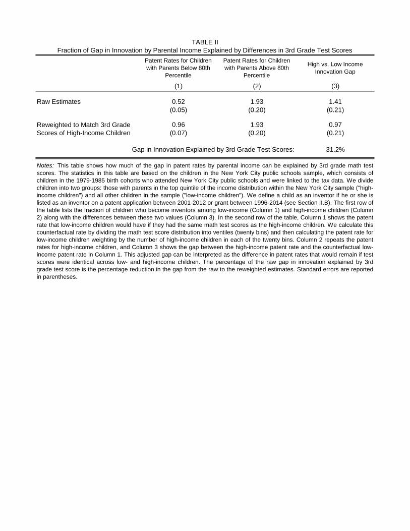
Patent Rates for Children

with Parents Below 80th

Percentile

Patent Rates for Children

with Parents Above 80th

Percentile

High vs. Low Income

Innovation Gap

(1) (2) (3)

Raw Estimates 0.52 1.93 1.41

(0.05) (0.20) (0.21)

0.96 1.93 0.97

(0.07) (0.20) (0.21)

31.2%

TABLE II

Fraction of Gap in Innovation by Parental Income Explained by Differences in 3rd Grade Test Scores

Reweighted to Match 3rd Grade

Scores of High-Income Children

Notes: This table shows how much of the gap in patent rates by parental income can be explained by 3rd grade math test

scores. The statistics in this table are based on the children in the New York City public schools sample, which consists of

children in the 1979-1985 birth cohorts who attended New York City public schools and were linked to the tax data. We divide

children into two groups: those with parents in the top quintile of the income distribution within the New York City sample ("high-

income children") and all other children in the sample ("low-income children"). We define a child as an inventor if he or she is

listed as an inventor on a patent application between 2001-2012 or grant between 1996-2014 (see Section II.B). The first row of

the table lists the fraction of children who become inventors among low-income (Column 1) and high-income children (Column

2) along with the differences between these two values (Column 3). In the second row of the table, Column 1 shows the patent

rate that low-income children would have if they had the same math test scores as the high-income children. We calculate this

counterfactual rate by dividing the math test score distribution into ventiles (twenty bins) and then calculating the patent rate for

low-income children weighting by the number of high-income children in each of the twenty bins. Column 2 repeats the patent

rates for high-income children, and Column 3 shows the gap between the high-income patent rate and the counterfactual low-

income patent rate in Column 1. This adjusted gap can be interpreted as the difference in patent rates that would remain if test

scores were identical across low- and high-income children. The percentage of the raw gap in innovation explained by 3rd

grade test score is the percentage reduction in the gap from the raw to the reweighted estimates. Standard errors are reported

in parentheses.

Gap in Innovation Explained by 3rd Grade Test Scores:

(1) (2) (3) (4) (5)

Fraction

Inventing

Fraction Inventing

in Patent Category

Fraction Inventing

in Patent

Sub-Category

Fraction Inventing

in Patent Class

Fraction Inventing

in Patent Class

0.250

(0.028)

0.163

(0.018)

0.155

(0.017)

0.078 0.0598

(0.013) (0.0125)

0.0044

(0.0008)

0.0001

(0.0004)

0.0002

(0.0000)

Fixed Effects None Patent Category Patent

Sub-Category

Patent Class Patent Class

Unit of Observation Father's Industry Father's Industry

by Patent

Category

Father's Industry

by Patent Sub-

Category

Father's Industry

by Patent Class

Father's Industry

by Patent Class

Number of Cells 345 2,415 12,765 153,525 153,525

TABLE III

Exposure to Innovation from Parents' Colleagues: Children's Innovation Rates vs. Patent Rates in Father's Industry

Notes: This table analyzes how a child's propensity to invent is related to patent rates in his or her father's industry. The sample consists of

children in the intergenerational sample (1980-84 birth cohorts) whose parents are not inventors. Each column presents estimates from a

separate OLS regression, with standard errors clustered by industry in parentheses. In Column 1, we regress the share of children who become

inventors among those with fathers in industry j on the patent rate among workers in industry j , with one observation per industry (six digit NAICS

code). We measure the patent rate among workers in each industry as the average number of patents issued to individuals in that industry per

year between 1996-2012 divided by the average number of workers per year (based on W-2 counts) in each industry between 1999-2012.

Column 2 is run at the industry by patent category level. Here, we regress the share of children with fathers in industry j who invent in patent

category c on the share of workers in industry j who have patents in category c . We include patent category fixed effects in this regression to

account for differences in patent rates across categories. Columns 3 and 4 are analogous to Column 2, but use more narrowly defined

categorizations of patent types: patent sub-categories and patent classes. Column 5 replicates Column 4 with three additional controls: the

fraction of inventors in (i) the same sub-category but in a different patent class, (ii) the same category but a different sub-category, and (iii) other

categories. All regressions are weighted by the number of children in each cell. There are 10,213,731 children underlying these regressions, the

set of children in the intergenerational sample whose fathers have a non-missing NAICS code.

Patent Rate in Father's Industry

Patent Rate in Father's Industry

in Same Category

Patent Rate in Father's Industry

in Same Sub-Category

Patent Rate in Father's Industry

in Same Class

Patent Rate in Father's Industry

in Same Sub-Category but Other

Class

Patent Rate in Father's Industry

in Same Category but Other Sub-

Category

Patent Rate in Father's Industry

in Other Category

Dependent Variable:

(1) (2) (3) (4) (5) (6) (7) (8)

Fraction

Inventing

Fraction

Inventing

Fraction

Inventing

in Patent

Category

Fraction

Inventing

in Patent

Category

Fraction

Inventing

in Patent

Category

Fraction

Inventing

in Patent

Sub-Cat.

Fraction

Inventing

in Patent

Class

Fraction

Inventing

in Patent

Class

2.932 2.578

(0.417) (0.531)

1.759 1.114 1.722

(0.404) (0.341) (0.406)

1.526

(0.375)

1.108 1.017

(0.181) (0.162)

0.0003

(0.0063)

-0.0015

(0.0028)

0.0054

(0.0006)

Fixed Effects None Current CZ Category Current CZ by

Category

Father's

NAICS by

Category

Sub-

Category

Class Class

Unit of observation Childhood CZ Childhood CZ

by Current CZ

Childhood CZ

by Category

Childhood CZ

by Current CZ

by Category

Childhood CZ

by Father's

NAICS

by Category

Childhood CZ

by Sub-Category

Childhood CZ

by Patent

Class

Childhood CZ

by Patent Class

Number of Cells 741 221,621 5,187 1,551,347 1,637,706 27,417 329,745 329,745

TABLE IV

Neighborhood Exposure Effects: Children's Innovation Rates vs. Patent Rates in Childhood Commuting Zone

Notes: This table analyzes how a child's propensity to invent is related to patent rates in his or her childhood commuting zone. The sample consists of children

in the intergenerational sample (1980-84 birth cohorts) whose parents are not inventors. Each child is assigned a childhood CZ based on the ZIP code from

which their parents first claimed them as dependents. Each column presents estimates from a separate OLS regression, with standard errors clustered by CZ

in parentheses. In Column 1, we regress the share of children who become inventors among those who grow up in CZ j on the patent rate among workers in

CZ j , with one observation per CZ. We measure the patent rate among workers in each CZ as the average number of patents issued per year (in the full

USPTO data) to individuals in a given CZ between 1980 and 1990 divided by the CZ's population between the ages of 15-64 in the 1990 Census. Column 2 is

run at the childhood CZ by current CZ level, limiting the sample to children whose current (2012) CZ differs from their childhood CZ. Here, we regress the share

of inventors in each cell on the patent rate in the childhood CZ and on fixed effects for the 2012 CZ, so that the coefficient on childhood CZ patent rates is

identified from comparisons across individuals currently living in the same CZ. Column 3 is run at the childhood CZ by patent category level. Here, we regress

the share of children from CZ j who invent in patent category c on the share of workers in CZ j who have patents in category c . We include patent category

fixed effects in this regression to account for differences in patent rates across categories. Column 4 replicates Column 2 at the category level, limiting the

sample to children who move and estimating the model at the childhood CZ by current CZ by category level, with current CZ by category fixed effects. In

Column 5, we include all children and replace the CZ by category fixed effects with fixed effects for the father's industry by category, estimating the model at the

childhood CZ by father's industry by category level. This specification isolates variation from one's neighbors that is orthogonal to the variation from parents'

colleagues. Columns 6 and 7 are analogous to Column 3 but use more narrowly defined categorizations of patent types: patent sub-categories and patent

classes. Column 8 replicates Column 7 with three additional controls: the fraction of inventors in (i) the same sub-category but in a different patent class, (ii) the

same category but a different sub-category, and (iii) other categories. All regressions are weighted by the number of children in each cell. There are

approximately 15.5 million children underlying the regressions in Columns 1, 3, 6, 7 and 8. Columns 2 and 4 are based on the subset of 5.4 million individuals

who moved across CZs. Column 5 includes the 10.2 million children whose fathers have non-missing NAICS codes.

Patent Rate in Childhood

CZ

Patent Rate in Same

Category in Childhood

CZ

Patent Rate in Same

Sub-Category in

Childhood CZ

Patent Rate in Same

Technology Class in

Childhood CZ

Patent Rate in Same

Sub-Category, but

Different Technology

Class in Childhood CZ

Patent Rate in Different

Category of Childhood

CZ

Patent Rate in Same

Category, but Different

Sub-Category in

Childhood CZ

Dependent Variable:

(1) (2) (3) (4) (5)

Fraction

Inventing in

CZ

Fraction of

Women

Inventing

Fraction of Men

Inventing

Fraction of Women

Inventing in Patent

Category

Fraction of Men

Inventing in Patent

Category

0.986

(0.145)

2.408 -0.356 2.232 -2.157

(1.265) (4.398) (0.607) (1.300)

0.174 1.784 0.102 1.693

(0.154) (0.625) (0.062) (0.295)

Fixed Effects None None None Category Category

Unit of Observation Childhood CZ Childhood CZ Childhood CZ Childhood CZ

by Category

Childhood CZ

by Category

Number of Cells 741 741 741 5,188 5,188

0.113 0.667 0.001 0.015

TABLE V

Gender-Specific Exposure Effects: Children's Innovation Rates vs. Innovation Rates by Gender in Childhood CZ

Innovation Rate of Women

in Childhood CZ

Innovation Rate of Men

in Childhood CZ

Notes: This table analyzes how a child's propensity to invent is related to the innovation rates of adults of the same gender in his or her

childhood commuting zone (CZ). The sample consists of children in the intergenerational sample (1980-84 birth cohorts) whose parents are not

inventors. Each column presents estimates from a separate OLS regression, with standard errors clustered by CZ in parentheses. Column 1

replicates the specification in Column 1 of Table IV, except that here we define the independent variable using the linked patent-tax data rather

than just the patent data, since we do not observe gender in the patent data itself. Specifically, we define the innovation rate for workers in CZ j

as the total number of patent applications filed by individuals born before 1980 in our full inventors sample divided by the number of individuals

between ages 15 and 64 in CZ j in the 1990 Census. We convert this measure to an annual rate by dividing by 17, as we observe patents

between 1996-2012. In Column 2, we regress the fraction of girls from CZ j who become inventors on the patent rates of female and male

workers in CZ j . Column 3 replicates Column 2 using the share of boys who become inventors as the dependent variable. The regression in

column 4 is run at the childhood CZ by patent category level. Here, we regress the share of girls from CZ j who invent in patent category c on

the share of male and female workers in CZ j who have patents in category c . We include patent category fixed effects in this regression to

account for differences in patent rates across categories. Columns 5 replicates Column 4 using the share of boys who become inventors as the

dependent variable. All regressions are weighted by the number of children in each cell. The last row of the table reports p-values from F-tests

for equality of the coefficients on male and female innovation rates in each regression. There are 15,499,290 individuals underlying each of the

regressions.

Innovation Rate

in Childhood CZ

Dependent variable:

p-value from F-test for Equality

of Coefficients

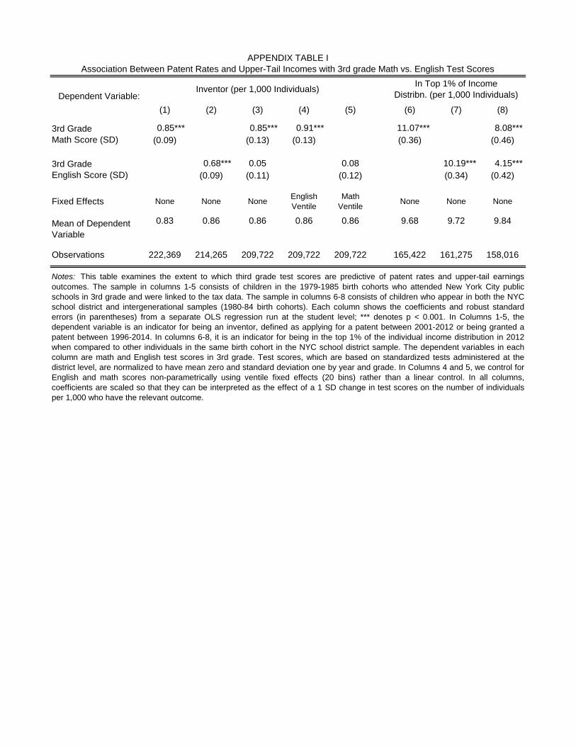
(1) (2) (3) (4) (5) (6) (7) (8)

0.85*** 0.85*** 0.91*** 11.07*** 8.08***

(0.09) (0.13) (0.13) (0.36) (0.46)

0.68*** 0.05 0.08 10.19*** 4.15***

(0.09) (0.11) (0.12) (0.34) (0.42)

Fixed Effects None None NoneEnglish

Ventile

Math

VentileNone None None

Mean of Dependent

Variable

0.83 0.86 0.86 0.86 0.86 9.68 9.72 9.84

Observations 222,369 214,265 209,722 209,722 209,722 165,422 161,275 158,016

Notes: This table examines the extent to which third grade test scores are predictive of patent rates and upper-tail earnings

outcomes. The sample in columns 1-5 consists of children in the 1979-1985 birth cohorts who attended New York City public

schools in 3rd grade and were linked to the tax data. The sample in columns 6-8 consists of children who appear in both the NYC

school district and intergenerational samples (1980-84 birth cohorts). Each column shows the coefficients and robust standard

errors (in parentheses) from a separate OLS regression run at the student level; *** denotes p < 0.001. In Columns 1-5, the

dependent variable is an indicator for being an inventor, defined as applying for a patent between 2001-2012 or being granted a

patent between 1996-2014. In columns 6-8, it is an indicator for being in the top 1% of the individual income distribution in 2012

when compared to other individuals in the same birth cohort in the NYC school district sample. The dependent variables in each

column are math and English test scores in 3rd grade. Test scores, which are based on standardized tests administered at the

district level, are normalized to have mean zero and standard deviation one by year and grade. In Columns 4 and 5, we control for

English and math scores non-parametrically using ventile fixed effects (20 bins) rather than a linear control. In all columns,

coefficients are scaled so that they can be interpreted as the effect of a 1 SD change in test scores on the number of individuals

per 1,000 who have the relevant outcome.

Inventor (per 1,000 Individuals)In Top 1% of Income

Distribn. (per 1,000 Individuals)

APPENDIX TABLE I

Association Between Patent Rates and Upper-Tail Incomes with 3rd grade Math vs. English Test Scores

Dependent Variable:

3rd Grade

Math Score (SD)

3rd Grade

English Score (SD)

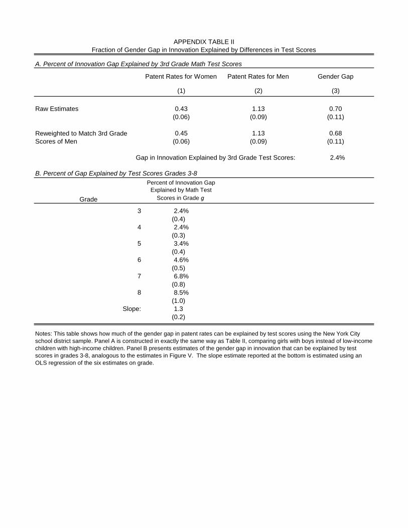
Patent Rates for Women Patent Rates for Men Gender Gap

(1) (2) (3)

Raw Estimates 0.43 1.13 0.70

(0.06) (0.09) (0.11)

0.45 1.13 0.68

(0.06) (0.09) (0.11)

2.4%

Grade

Percent of Innovation Gap

Explained by Math Test

Scores in Grade g

3 2.4%

(0.4)

4 2.4%

(0.3)

5 3.4%

(0.4)

6 4.6%

(0.5)

7 6.8%

(0.8)

8 8.5%

(1.0)

Slope: 1.3

(0.2)

B. Percent of Gap Explained by Test Scores Grades 3-8

APPENDIX TABLE II

Fraction of Gender Gap in Innovation Explained by Differences in Test Scores

A. Percent of Innovation Gap Explained by 3rd Grade Math Test Scores

Notes: This table shows how much of the gender gap in patent rates can be explained by test scores using the New York City

school district sample. Panel A is constructed in exactly the same way as Table II, comparing girls with boys instead of low-income

children with high-income children. Panel B presents estimates of the gender gap in innovation that can be explained by test

scores in grades 3-8, analogous to the estimates in Figure V. The slope estimate reported at the bottom is estimated using an

OLS regression of the six estimates on grade.

Reweighted to Match 3rd Grade

Scores of Men

Gap in Innovation Explained by 3rd Grade Test Scores:

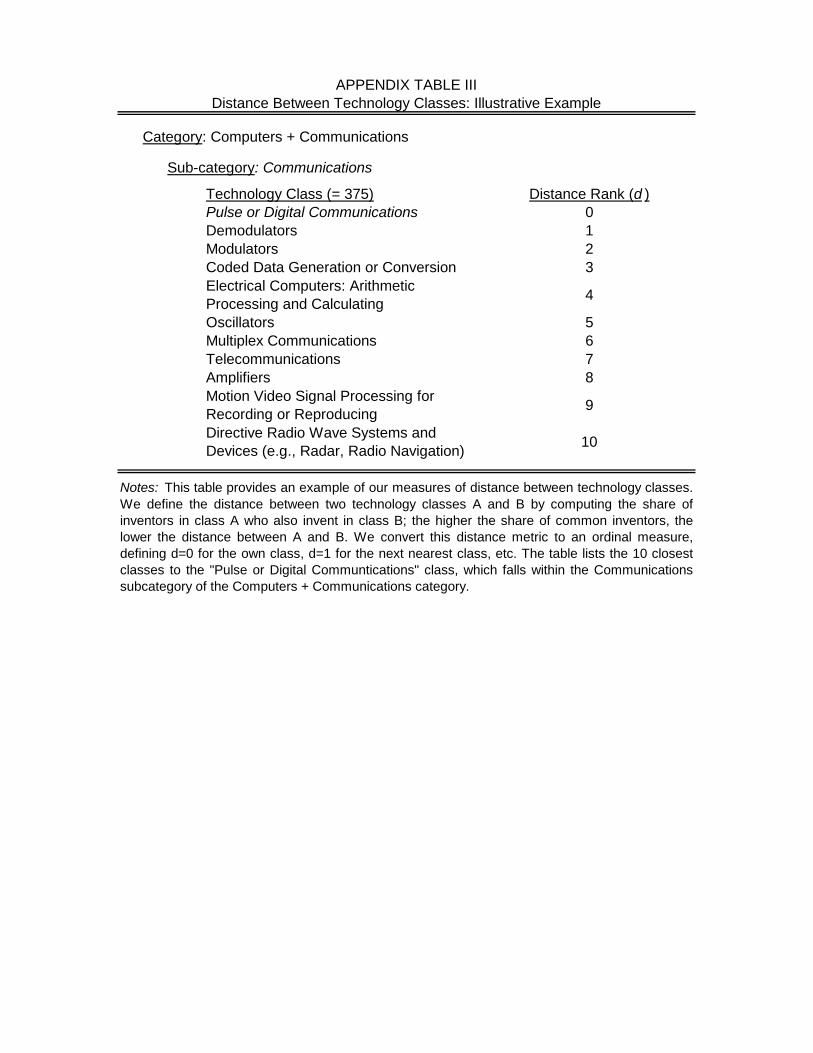
Technology Class (= 375) Distance Rank (d )

Pulse or Digital Communications 0

Demodulators 1

Modulators 2

Coded Data Generation or Conversion 3

Electrical Computers: Arithmetic

Processing and Calculating4

Oscillators 5

Multiplex Communications 6

Telecommunications 7

Amplifiers 8

Motion Video Signal Processing for

Recording or Reproducing9

Directive Radio Wave Systems and

Devices (e.g., Radar, Radio Navigation)10

Sub-category: Communications

Category: Computers + Communications

APPENDIX TABLE III

Distance Between Technology Classes: Illustrative Example

Notes: This table provides an example of our measures of distance between technology classes.

We define the distance between two technology classes A and B by computing the share of

inventors in class A who also invent in class B; the higher the share of common inventors, the

lower the distance between A and B. We convert this distance metric to an ordinal measure,

defining d=0 for the own class, d=1 for the next nearest class, etc. The table lists the 10 closest

classes to the "Pulse or Digital Communtications" class, which falls within the Communications

subcategory of the Computers + Communications category.

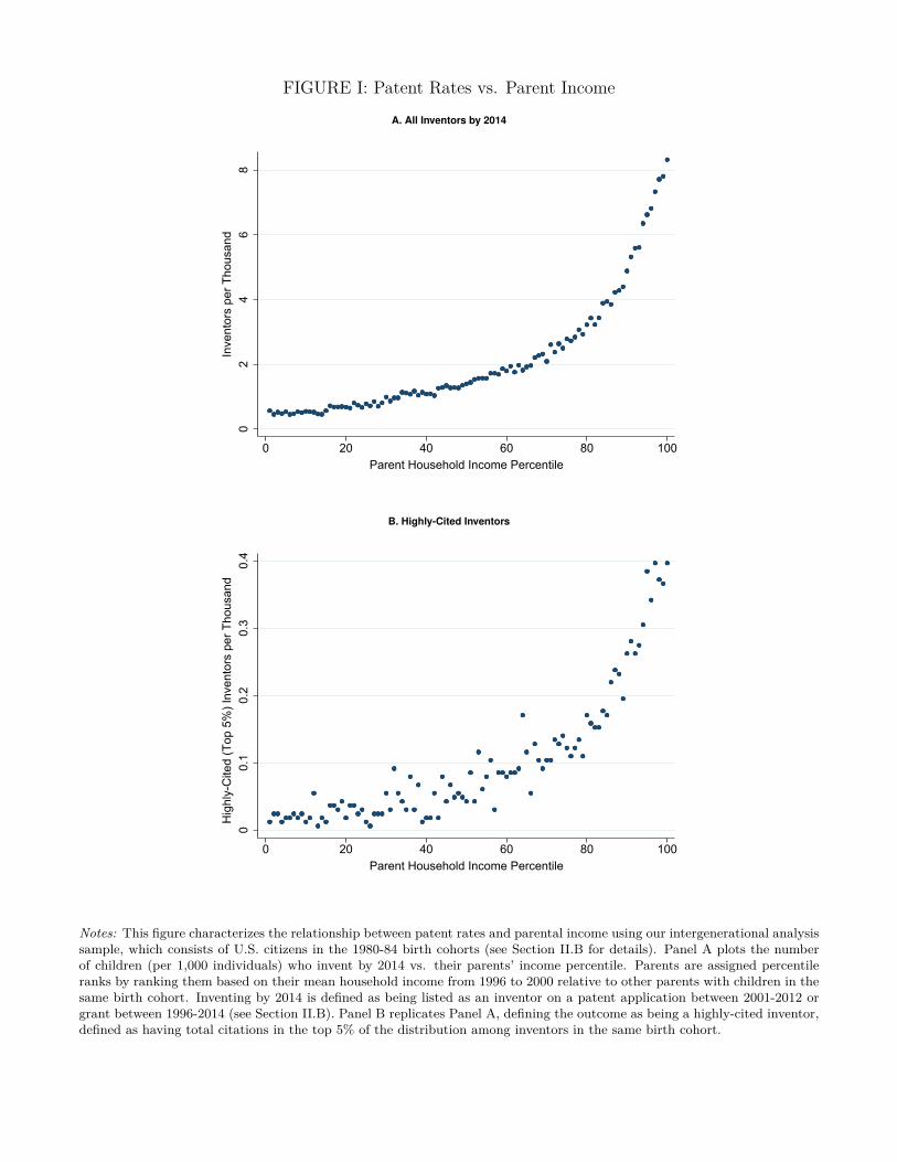
FIGURE I: Patent Rates vs. Parent IncomeA. All Inventors by 2014

02

46

8In

vent

ors

per T

hous

and

0 20 40 60 80 100Parent Household Income Percentile

B. Highly-Cited Inventors

00.

10.

20.

30.

4H

ighl

y-C

ited

(Top

5%

) Inv

ento

rs p

er T

hous

and

0 20 40 60 80 100Parent Household Income Percentile

Notes: This figure characterizes the relationship between patent rates and parental income using our intergenerational analysissample, which consists of U.S. citizens in the 1980-84 birth cohorts (see Section II.B for details). Panel A plots the numberof children (per 1,000 individuals) who invent by 2014 vs. their parents’ income percentile. Parents are assigned percentileranks by ranking them based on their mean household income from 1996 to 2000 relative to other parents with children in thesame birth cohort. Inventing by 2014 is defined as being listed as an inventor on a patent application between 2001-2012 orgrant between 1996-2014 (see Section II.B). Panel B replicates Panel A, defining the outcome as being a highly-cited inventor,defined as having total citations in the top 5% of the distribution among inventors in the same birth cohort.

FIGURE II: Patent Rates by Race and Ethnicity

1.6 1.6 1.6

0.5

1.0

0.6

0.20.3 0.3

3.3

4.2

3.1

01

23

4

Inven

tors

per

Th

ou

sand

White

Non-Hispanic

Black

Non-Hispanic

Hispanic Asian

Raw rate

Reweighted to

match parental

incomes of whites

Reweighted to match

3rd grade test scores

of whites

Notes: This figure presents patent rates by race and ethnicity using our New York City public schools sample, which consistsof children in the 1979-1985 birth cohorts who attend NYC public schools at some point between grades 3-8. Each bar plotsthe number of children (per 1,000 individuals) who invent by 2014, as defined in the notes to Figure I. In each triplet, the firstbar shows the raw patent rate for the relevant subgroup. The second bar plots the patent rate that would prevail if children inthe relevant subgroup had the same distribution of parental income as white children. To construct these estimates, we dividechildren into 20 bins based on their parental incomes and compute mean patent rates across the 20 bins, weighting each binby the fraction of white children with incomes in that bin. The third bar in each triplet shows the patent rate that wouldprevail if children in the relevant subgroup had the same distribution of 3rd grade math test scores as white children. Theseestimates are constructed by dividing children into 20 bins based on their test scores and computing mean patent rates acrossthe 20 bins, weighting each bin by the fraction of white children with test scores in that bin.

FIGURE III: Percentage of Female Inventors by Birth Cohort

Average change per year: 0.27%(0.01%)

01

02

03

04

05

0

Perc

enta

ge o

f In

vento

rs w

ho a

re F

em

ale

1940 1950 1960 1970 1980

Year of Birth

118 years to reach 50% female share

Notes: This figure plots the percentage of inventors who are female by year of birth using our full inventors sample, whichconsists of all 1.2 million individuals in the linked patent-tax data. Inventing is defined as being listed as an inventor ona patent application between 2001-2012 or grant between 1996-2014 (see Section II.B for details). The change per year isestimated using an unweighted OLS regression of the percentage of female inventors on birth year, depicted by the solid line.The standard error from this regression is shown in parentheses.

FIGURE IV: Patent Rates vs. 3rd Grade Math Test Scores

A. By Parental Income

90th Percentile

02

46

8In

vent

ors

per T

hous

and

-2 -1 0 1 23rd Grade Math Test Score (Standardized)

Parent Income Below 80th Percentile Parent Income Above 80th Percentile

B. By Race and Ethnicity

90th Percentile

02

46

8In

vent

ors

per T

hous

and

-2 -1 0 1 23rd Grade Math Test Score (Standardized)

Hispanic Black White Asian

C. By Gender

90th Percentile

02

46

8In

vent

ors

per T

hous

and

-2 -1 0 1 23rd Grade Math Test Score (Standardized)

Female Male

Notes: This figure shows the relationship between patent rates and math test scores in 3rd grade for various subgroups. Thesample consists of children in the 1979-1985 birth cohorts who attended New York City public schools in 3rd grade. Testscores, which are based on standardized tests administered at the district level, are normalized to have mean zero and standarddeviation one by year and grade. In Panel A, we divide children into two groups based on whether their parents’ incomesfall below the 80th percentile of the income distribution of parents’ income in the New York City schools sample. The figurepresents a binned scatter plot of patent rates vs. test scores for these two subgroups. To construct the figure, we first dividechildren into 20 equal sized bins (ventiles) based on their test scores. We then plot the share of inventors (per 1000 individuals)vs. the mean test score within each bin for each of the two subgroups. Panel B and C replicate Panel A, dividing children bytheir race and ethnicity (Panel B) and gender (Panel C) instead of parental income. We use 10 bins rather than 20 bins oftest scores in Panel B because of smaller sample sizes for some racial and ethnic groups. The vertical dashed lines depict the90th percentile of the test-score distribution.

FIGURE V: Gap in Patent Rates by Parental Income Explained by Test Scores in Grades 3-8

Slope: 3.20% (0.55)

3035

4045

50Pe

rcen

t of G

ap E

xpla

ined

by

Mat

h Te

st S

core

s

3 4 5 6 7 8Grade

Notes: This figure shows how much of the gap in patent rates by parental income can be explained by math test scores ingrades 3-8. The sample consists of children in our New York City public schools sample (birth cohorts 1979-1985), whom wedivide into two groups: those with parents in the top quintile of the income distribution within the New York City sample(“high-income children”) and all other children in the sample (“low-income children”). The gap in innovation explained bymath test scores in grade g is the percentage reduction in the gap in innovation when we reweight low-income students’ gradeg test score distribution to match that of high-income students. Table II illustrates how we construct this estimate using 3rdgrade test scores (31.2%); estimates for later grades use the same methodology. The slope and best-fit line are estimated usingan unweighted OLS regression on the six points, with standard error reported in parentheses.

FIGURE VI: Children’s Patent Rates vs. Class-Level Patent Rates in Childhood Environment

A. Patent Rates by Distance from Father’s Technology Class for

Children of Inventors

0

0.2

0.4

0.6

0.8

1

Inve

ntor

s pe

r Tho

usan

d

0 20 40 60 80 100Distance from Father's Technology Class

B. Effects of Class-Level Patent Rates in Father’s Industry

by Technological Distance

00.

020.

040.

060.

08R

egre

ssio

n C

oeffi

cien

t on

Cla

ss-L

evel

Pat

ent R

ate

0 1-10 11-20 21-30 31-40 41-50 51-60 61-70 71-80 81-90 91-100Distance Between Technology Classes

C. Effects of Class-Level Patent Rates in Childhood CZ

by Technological Distance

00.

20.

40.

60.

81

1.2

Reg

ress

ion

Coe

ffici

ent o

n C

lass

-Lev

el P

aten

t Rat

e

0 1-10 11-20 21-30 31-40 41-50 51-60 61-70 71-80 81-90 91-100Distance Between Technology Classes

Notes: This figure shows how children’s propensities to patent in a technology class vary with the class in which their father(Panel A), father’s colleagues (Panel B), or childhood neighbors (Panel C) patented. In Panel A, the sample consists of allchildren in our intergenerational sample whose fathers are inventors (those who applied for a patent between 2001-2012 orwere granted a patent between 1996-2014) and who were not listed as co-inventors on a patent with their fathers. To constructPanel A, we first assign fathers and children a technology class based on the class in which they have the most patents andpatent applications. We then define the distance between two technology classes A and B based on the share of inventors inclass A who also invent in class B. Using this distance metric, for each child, we define d = 0 as the class in which his or herfather patents, d = 1 as the next closest class, etc. We then plot the share of children (per 1,000 individuals) who invent in atechnology class that is d units away from their father’s class. Classes in which fewer than 100 inventors have a patent grantor application between 1996-2014 are omitted. In Panels B and C, the sample consists of all children in our intergenerationalsample whose parents are not inventors. Each bar in Panel B plots estimates from a separate regression, with one observationper father’s industry (six digit NAICS code) and patent technology class. In the first bar, we regress the fraction of childrenwho patent in technology class c among those with fathers in industry j on the patent rate among workers in industry j inthe same technology class c. We measure the class-level patent rate among workers in each industry as the average numberof patents in class c issued to individuals in that industry per year (between 1996-2012) divided by the average number ofworkers per year in each industry between 1999-2012. In the second bar, we regress the same dependent variable on the meanpatent rate in the father’s industry in the 10 closest classes (d = 1 to 10). The third bar uses the average patent rate inclasses with d = 11 to 20, etc. All regressions are weighted by the number of children in each cell and include class level fixedeffects for class c. Panel C replicates Panel B, replacing patent rates in the father’s industry with patent rates of workers inthe CZ where the child grew up. CZ-level patent rates are defined as the average number of patents issued in class c per yearto individuals from a given CZ between 1980-1990 divided by the CZ’s population between ages 15-64 in the 1990 Census.

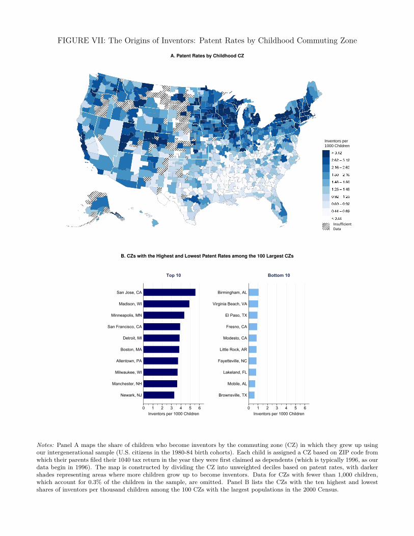
FIGURE VII: The Origins of Inventors: Patent Rates by Childhood Commuting Zone

A. Patent Rates by Childhood CZ

Inventors per

1000 Children

Insufficient Data

B. CZs with the Highest and Lowest Patent Rates among the 100 Largest CZs

0 1 2 3 4 5 6Inventors per 1000 Children

Newark, NJ

Manchester, NH

Milwaukee, WI

Allentown, PA

Boston, MA

Detroit, MI

San Francisco, CA

Minneapolis, MN

Madison, WI

San Jose, CA

Top 10

0 1 2 3 4 5 6Inventors per 1000 Children

Brownsville, TX

Mobile, AL

Lakeland, FL

Fayetteville, NC

Little Rock, AR

Modesto, CA

Fresno, CA

El Paso, TX

Virginia Beach, VA

Birmingham, AL

Bottom 10

Notes: Panel A maps the share of children who become inventors by the commuting zone (CZ) in which they grew up usingour intergenerational sample (U.S. citizens in the 1980-84 birth cohorts). Each child is assigned a CZ based on ZIP code fromwhich their parents filed their 1040 tax return in the year they were first claimed as dependents (which is typically 1996, as ourdata begin in 1996). The map is constructed by dividing the CZ into unweighted deciles based on patent rates, with darkershades representing areas where more children grow up to become inventors. Data for CZs with fewer than 1,000 children,which account for 0.3% of the children in the sample, are omitted. Panel B lists the CZs with the ten highest and lowestshares of inventors per thousand children among the 100 CZs with the largest populations in the 2000 Census.

FIGURE VIII: Children’s Patent Rates vs. Patent Rates of Workers in their Childhood CZ

Newark

Houston

Minneapolis

San Jose

Brownsville

Portland

Madison

01

23

45

6N

um. o

f Inv

ento

rs p

er 1

000

Chi

ldre

n w

ho G

row

up

in C

Z

0 0.2 0.4 0.6 0.8Annual Patent Rate per Thousand Working Age Adults in CZ

Notes: The figure plots the patent rates of children who grow up in a given CZ (constructed exactly as in Figure VII) vs.the patent rates of workers who live in that CZ. Patent rates of workers in each CZ are defined as the average number ofpatents per year issued to inventors residing in that CZ between 1980-1990 (based on the universe of USPTO data) dividedby the CZ’s population between the ages of 15-64 in the 1990 Census. We restrict the figure to the 100 CZs with the largestpopulations. The solid best-fit line is estimated using an unweighted OLS regression on these 100 observations (slope = 4.22,standard error = 0.40).

FIGURE IX: Geographical Variation in Gender Gaps in Patent Rates

A. Percent of Inventors who are Female by State where Child Grew Up

> 20.4

< 14.7

Share of Female

Inventors (%)

B. CZs with the Highest and Lowest Female Inventor Shares Among the 100 Largest CZs

0 10 20 30 40 50Female Inventor Share (%)

Dayton, OH

Charlotte, NC

Brownsville, TX

Cape Coral, FL

Greenville, SC

Jacksonville, FL

Lakeland, FL

Toms River, NJ

Honolulu, HI

Modesto, CA

Top 10

0 10 20 30 40 50Female Inventor Share (%)

Santa Rosa, CA

Little Rock, AR

Oklahoma City, OK

Fresno, CA

Bakersfield, CA

Erie, PA

Fayetteville, NC

Grand Rapids, MI

Salt Lake City, UT

Eugene, OR

Bottom 10

Notes: Panel A maps the percentage of female inventors by the state in which they grew up using our intergenerational sample(U.S. citizens in the 1980-84 birth cohorts). Each child is assigned a state based on ZIP code from which their parents filedtheir 1040 tax return in the year they were first claimed as dependents (which is typically 1996, as our data begin in 1996).The map is constructed by dividing the states into unweighted quintiles based on the female inventor share, with darker shadesrepresenting areas where women account for a larger share of inventors. Panel B lists the commuting zones (CZs) with theten highest and lowest female inventor shares among the 100 CZs with the largest populations in the 2000 Census.

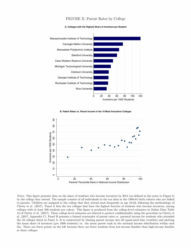
FIGURE X: Patent Rates by College

A. Colleges with the Highest Share of Inventors per Student

0 20 40 60 80 100 120Inventors per 1000 Students

Rice University

Rochester Institute of Technology

Georgia Institute of Technology

Clarkson University

Michigan Technological University

Case Western Reserve University

Stanford University

Rensselaer Polytechnic Institute

Carnegie Mellon University

Massachusetts Institute of Technology

B. Patent Rates vs. Parent Income in the 10 Most Innovative Colleges

010

2030

4050

6070

8090

Inve

ntor

s pe

r 100

0 St

uden

ts

0 20 40 60 80 100Parents' Percentile Rank in National Income Distribution

Notes: This figure presents data on the share of students who become inventors by 2014 (as defined in the notes to Figure I)by the college they attend. The sample consists of all individuals in the tax data in the 1980-84 birth cohorts who are linkedto parents. Children are assigned to the college that they attend most frequently at age 19-22, following the methodology ofChetty et al. (2017). Panel A lists the ten colleges that have the highest fraction of students who become inventors, amongcolleges with at least 500 students per cohort. This figure is produced from the college-level estimates in Online Data Table12 of Chetty et al. (2017). These college-level estimates are blurred to protect confidentiality using the procedure in Chetty etal. (2017, Appendix C). Panel B presents a binned scatterplot of patent rates vs. parental income for students who attendedthe 10 colleges listed in Panel A. It is constructed by binning parent income into 20 equal-sized bins (ventiles) and plottingthe mean share of inventors (per 1000 students) vs. the mean parent rank in the national income distribution within eachbin. There are fewer points on the left because there are fewer students from low-income families than high-income familiesat these colleges.

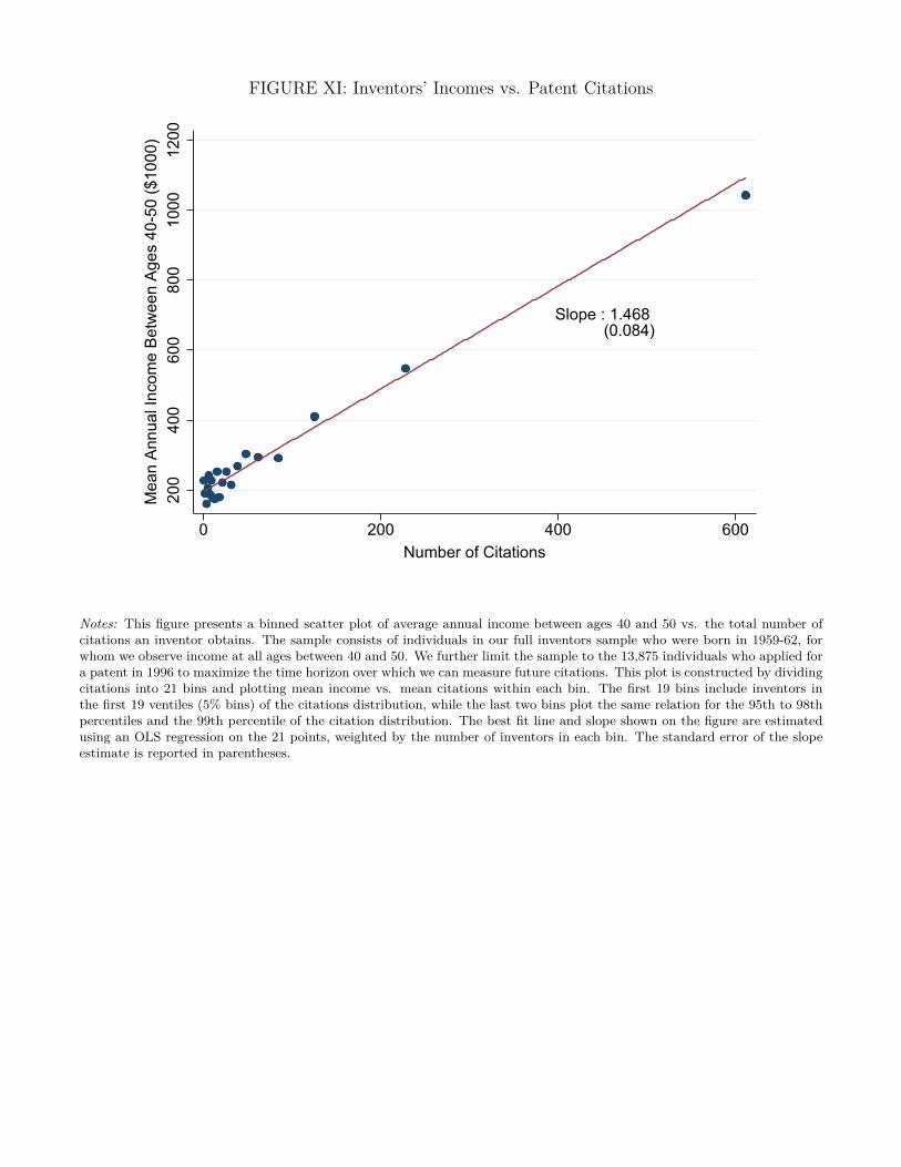
FIGURE XI: Inventors’ Incomes vs. Patent Citations

Slope : 1.468 (0.084)

200

400

600

800

1000

1200

Mea

n An

nual

Inco

me

Betw

een

Ages

40-

50 ($

1000

)

0 200 400 600Number of Citations

Notes: This figure presents a binned scatter plot of average annual income between ages 40 and 50 vs. the total number ofcitations an inventor obtains. The sample consists of individuals in our full inventors sample who were born in 1959-62, forwhom we observe income at all ages between 40 and 50. We further limit the sample to the 13,875 individuals who applied fora patent in 1996 to maximize the time horizon over which we can measure future citations. This plot is constructed by dividingcitations into 21 bins and plotting mean income vs. mean citations within each bin. The first 19 bins include inventors inthe first 19 ventiles (5% bins) of the citations distribution, while the last two bins plot the same relation for the 95th to 98thpercentiles and the 99th percentile of the citation distribution. The best fit line and slope shown on the figure are estimatedusing an OLS regression on the 21 points, weighted by the number of inventors in each bin. The standard error of the slopeestimate is reported in parentheses.

FIGURE XII: Age Profile of Innovation

A. Age Distribution of Individuals who Patent in 2000

00.

010.

020.

030.

04D

ensi

ty

20 30 40 50 60 70Age

B. Fraction of Workers who Patent in 2000, by Age

00.

51

1.5

22.

5W

orke

rs w

ho P

aten

t in

2000

(per

10,

000)

20 30 40 50 60Age

C. Fraction of Workers with Highly-Cited Patents, by Age

00.

050.

100.

15W

orke

rs w

ith H

ighl

y C

ited

Pate

nts

in 2

000

(per

10,

000)

20 30 40 50 60Age

Notes: This figure examines the age distribution of inventors. The sample consists of individuals in our full inventors samplewho applied for a patent in 2000 that was subsequently granted. Panel A presents a kernel density of the age distribution ofthese inventors. Panel B plots the fraction of workers (individuals with positive W-2 earnings) who patent in 2000 by age.Panel C plots the fraction of workers who filed a patent application in 2000 that went on to become highly-cited (in the top5% of the distribution). The curves in Panels B and C are cubic splines.

12

FIGURE XIII: Income Profiles of Inventors

A. Median Income by Age

2040

6080

100

120

Med

ian

Inco

me

($10

00)

20 30 40 50 60Age

Patent App. at Age 30 Patent App. at Age 40 Patent App. at Age 50

B. Event Study of Income Distributions Around Patent Application

800

1000

1200

1400

1600

1800

99th

Per

cent

ile o

f Inc

ome

Dis

tribu

tion

($10

00)

5010

015

020

0M

edia

n or

Mea

n In

com

e ($

1000

)

-10 -5 0 5 10Year Relative to Patent Application

Median Income Mean Income 99th Percentile

C. Event Study of Median Income around Patent Application, by

Patent Quality

6080

100

120

140

Med

ian

Inco

me

($10

00)

-10 -5 0 5 10Year Relative to Patent Application

Ungranted Patents Granted Patents Highly-Cited (Top 5%) Patents

Notes: This figure plots the income profiles of inventors before and after they file patent applications using all individualsfor whom the relevant data is available in our full inventors sample. Income is measured as total income (including wageearnings and capital income) at the individual level; see Section II.C for details. Panel A plots the median incomes by age ofinventors who file a patent application at either age 30, 40, or 50 over the range of ages for which their incomes are observed(between 1996-2012). Panel B generalizes this analysis using an event study framework, defining year 0 as the year in which anindividual files a patent application and other years relative to this reference year (e.g., +1 is the year after the application).In this figure, we limit the sample to individuals who file patent applications between ages 35 and 50. For individuals whofile multiple patents in this age window, we choose one of the patents at random to define the reference year. We plot themean and median (left y axis) and 99th percentile (right y axis) of the income distribution of inventors in each year relative tothe event year. Panel C replicates the median income series in Panel B, separating inventors into three groups: those whosepatent applications were not granted; those whose applications were granted; and those with patents granted that went on tohave citations in the top 5% of the distribution relative to other patents granted in the same year.

13

FIGURE XIV: Income and Citations of Inventors by Characteristics at BirthA. Mean Income

241

143

261224

122

193

010

020

030

040

0M

ean

Inco

me

in 2

012

($10

00)

Par Inc.Above p80

Par Inc.Below p80

Non-Minority Minority Male Female

B. Fraction with Highly-Cited Patents

5.75.2 5.4

2.6

4.85.3

02

46

810

Pct.

of In

vent

ors

in T

op 5

% o

f Cita

tion

Dis

tribu

tion

Par Inc.Above p80

Par Inc.Below p80

Non-Minority Minority Male Female

Notes: Panel A plots the mean incomes of inventors in 2012 by their parents’ income, race/ethnicity, and gender. The firstpair of bars uses our intergenerational sample (1980-84 birth cohorts), divided into two subgroups based on whether parents’household income is below or above the 80th percentile of the parent income distribution. The second pair of bars uses ourNew York City schools sample, divided into two subgroups based on race and ethnicity: minorities (Blacks and Hispanics)and non-Minorities. The third pair of bars uses our full inventors sample, divided by gender. The vertical lines depict 95%confidence intervals. Panel B replicates Panel A using the fraction of highly-cited inventors as the outcome. Highly-citedinventors are defined as inventors whose patents have citations per co-author in the top 5% of the distribution among thosein their birth cohort.

FIGURE XV: Predicted Impacts of Tax Rates on Innovation

A. Forecastable Returns

020

4060

8010

0%

Rel

ativ

e to

Bas

elin

e

0 10 20 30 40 50 60 70 80 90Tax Rate on Inventors' Earnings (%)

Quality-Weighted Aggregate Innovation (Φ)

Number of Inventors (φ)

B. Stochastic Returns

020

4060

8010

0%

Rel

ativ

e to

Bas

elin

e

0 10 20 30 40 50 60 70 80 90Tax Rate on Inventors' Earnings (%)

Quality-Weighted Aggregate Innovation (Φ), CRRA = 1

Number of Inventors (φ), CRRA = 1

Quality-Weighted Aggregate Innovation (Φ), CRRA = 0

Number of Inventors (φ), CRRA = 0

Notes: This figure plots the fraction of inventors (φ) and aggregate quality-weighted innovation (Φ) vs. the tax rate oninventors’ earnings predicted by the model of career choice in Section VI. Panel A considers the case where the variationin private financial returns to innovation is driven purely by differences in ability across inventors and hence is perfectlyforecastable at the time of career choice. Panel B considers the case where the variance in private returns come primarilyfrom stochastic shocks, with a coefficient of relative risk aversion θ = 0 (linear utility) or 1 (log utility). The shape parametersfor the Pareto distributions of stochastic returns and innovation abilities, denoted βπ and βα in the model, are chosen suchthat the inventors’ earnings distribution generated by the model matches the Pareto shape parameter of 1.26 estimatedusing inventors’ empirical earnings distribution in Online Appendix Figure VI, i.e. such that βπ

βπ−1βαβα−1 = 1.26

1.26−1 . In Panel B,stochastic returns account for 90% of total skewness in inventors’ earnings, i.e. s ≡

(βπβπ−1 − 1

)/

(βαβα−1 − 1 + βπ

βπ−1 − 1)

= 0.9.In each series, the level of innovation is normalized to 100% when the tax rate is 0. The normalized values are invariant tothe other parameters of the model (wI , λ, and θ in Panel A).

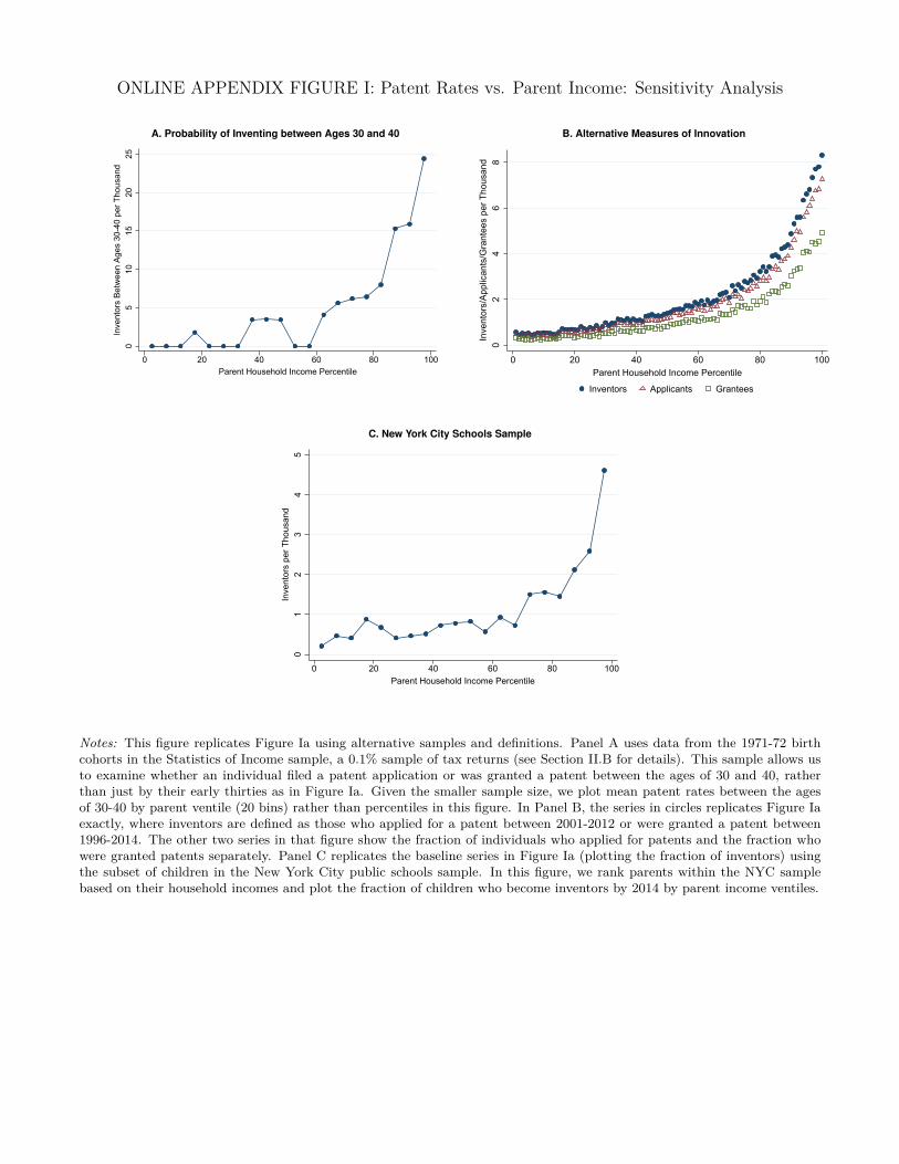
ONLINE APPENDIX FIGURE I: Patent Rates vs. Parent Income: Sensitivity Analysis

A. Probability of Inventing between Ages 30 and 400

510

1520

25In

vent

ors

Betw

een

Ages

30-

40 p

er T

hous

and

0 20 40 60 80 100Parent Household Income Percentile

B. Alternative Measures of Innovation

02

46

8In

vent

ors/

Appl

ican

ts/G

rant

ees

per T

hous

and

0 20 40 60 80 100Parent Household Income Percentile

Inventors Applicants Grantees

C. New York City Schools Sample

01

23

45

Inve

ntor

s pe

r Tho

usan

d

0 20 40 60 80 100Parent Household Income Percentile

Notes: This figure replicates Figure Ia using alternative samples and definitions. Panel A uses data from the 1971-72 birthcohorts in the Statistics of Income sample, a 0.1% sample of tax returns (see Section II.B for details). This sample allows usto examine whether an individual filed a patent application or was granted a patent between the ages of 30 and 40, ratherthan just by their early thirties as in Figure Ia. Given the smaller sample size, we plot mean patent rates between the agesof 30-40 by parent ventile (20 bins) rather than percentiles in this figure. In Panel B, the series in circles replicates Figure Iaexactly, where inventors are defined as those who applied for a patent between 2001-2012 or were granted a patent between1996-2014. The other two series in that figure show the fraction of individuals who applied for patents and the fraction whowere granted patents separately. Panel C replicates the baseline series in Figure Ia (plotting the fraction of inventors) usingthe subset of children in the New York City public schools sample. In this figure, we rank parents within the NYC samplebased on their household incomes and plot the fraction of children who become inventors by 2014 by parent income ventiles.

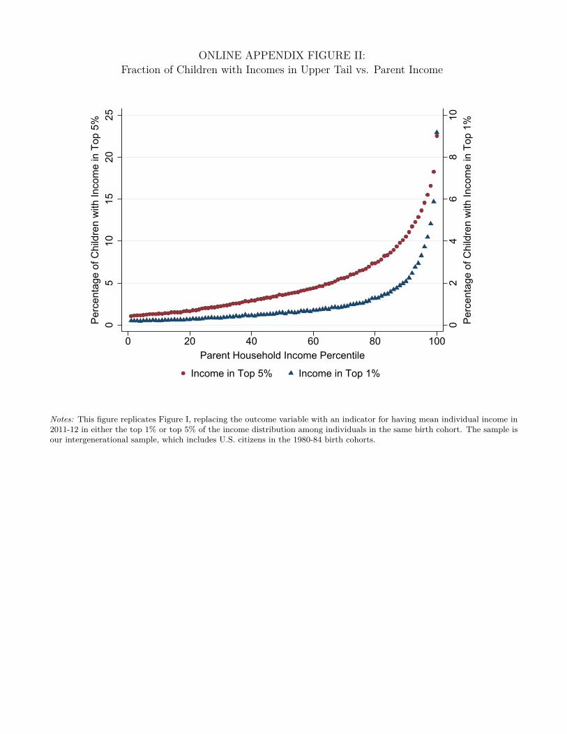
ONLINE APPENDIX FIGURE II:Fraction of Children with Incomes in Upper Tail vs. Parent Income

02

46

810

Perc

enta

ge o

f Chi

ldre

n w

ith In

com

e in

Top

1%

05

1015

2025

Perc

enta

ge o

f Chi

ldre

n w

ith In

com

e in

Top

5%

0 20 40 60 80 100Parent Household Income Percentile

Income in Top 5% Income in Top 1%

Notes: This figure replicates Figure I, replacing the outcome variable with an indicator for having mean individual income in2011-12 in either the top 1% or top 5% of the income distribution among individuals in the same birth cohort. The sample isour intergenerational sample, which includes U.S. citizens in the 1980-84 birth cohorts.

ONLINE APPENDIX FIGURE III: Distribution of Math Test Scores in 3rd Grade

A. By Parental Income

00.

10.

30.

50.

40.

2Den

sity

-3 -2 -1 0 1 2 3Grade 3 Math Scores (Standard Deviations Relative to Mean)

Parent IncomeBelow 80th Percentile

Parent IncomeAbove 80th Percentile

B. By Gender

00.

10.

30.

20.

4D

ensi

ty

-3 -2 -1 0 1 2 3Grade 3 Math Scores (Standard Deviations Relative to Mean)

Males Females

Notes: These figures present kernel densities of 3rd grade math test scores for children in the 1979-1985 birth cohorts whoattended New York City public schools. Test scores, which are based on standardized tests administered at the district level,are normalized to have mean zero and standard deviation one by year and grade. In Panel A, we divide children into twogroups based on whether their parents’ incomes fall below the 80th percentile of the income distribution of parents’ income inthe New York City schools sample. Panel B compares boys and girls.

3

ONLINE APPENDIX FIGURE IV: Female Inventor Share and Gender Stereotype Adherence

AK

AL

AR

AZCA

CO

CTDE

FLGA

HI

IA

ID

IL

INKS

KY

LA

MA MD

ME

MIMN

MO

MS

MT

NC

ND

NE

NH NJ

NM

NV

NYOH

OKOR

PA

RI

SC

SD

TNTX

UT

VA

VT

WAWI

WV

WY

1015

2025

30Pe

rcen

tage

of I

nven

tors

who

are

Fem

ale

1.5 2.0 2.5 3.0Gender Stereotype Adherence Index on 8th Grade Tests (Pope and Sydnor 2010)

Notes: This figure plots the share of inventors who are female vs. Pope and Syndor’s (2010) gender stereotype adherenceindex by state. Female inventor shares are taken directly from Figure IXa; see notes to that figure for details. The stereotypeadherence index is computed as S = (Nm,math&science/Nf,math&science+Nf,reading/Nm,reading)/2, where Ng,s denotes the numberof students of gender g∈ {m, f} who score among the top 5% of students in their state in subject s ∈ {math & science, reading}in 8th grade. The index S measures the degree to which students adhere to the typical gender stereotype that boys do betterat math/science and girls do better in reading; higher values represent greater adherence to this stereotype. The solid best-fitline is estimated using an unweighted OLS regression (slope = -4.49, standard error = 1.42).

ONLINE APPENDIX FIGURE V: Inventors’ Income Distribution

p50 = $114k p95 = $497 p99 = $1.6m0

0.00

20.

004

0.00

6D

ensi

ty

0 500 1000 1500Mean Annual Individual Income ($1000), Ages 40-50

Notes: This figure plots a kernel density of the distribution of inventors’ income, measured as mean annual income over ages40-50 in 2012 dollars. Income is measured at the individual level and includes both labor and capital income. The sampleconsists of all individuals in our full inventors sample born between the ages of 1959-1962, for whom we see income at allages between 40 and 50. For scaling purposes, the top and bottom percentiles of the distribution are omitted. The dashedlines mark the median, 95th percentile, and 99th percentile of the distribution.