who ate the capital? allocating sa-ccr fairly · who ate the capital? allocating sa-ccr fairly 1 1....

WHITE PAPER

WHO ATE THE CAPITAL? ALLOCATING SA-CCR FAIRLY

Who ate the capital? Allocating SA-CCR Fairly 1

1. Introduction The content of the the Basel Committee’s standardised approach for measuring counterparty credit risk exposures (SA-CCR) regulation has been known for some time now (see [1] or [2]). There are still some grey areas around the interpretation [3] but by and large, most banks have started to work on integrating SA-CCR as a measure into their risk or finance architectures. Calculating the overall impact is one issue. Understanding which parts of the portfolio cause the impact is another. The latter requires that the SA-CCR result be allocated back to transactions. Ranking counterparty portfolios by capital charge is a start, but we can slice portfolios by other dimensions, for instance by transaction type or dealing desk. Under the old Current Exposure Method (CEM) regulation, breaking the capital charge down by transaction was theoretically obvious and computationally trivial. Ignoring the net-to-gross ratio (NGR) for a moment, the capital charges are calculated per transaction and then added up. Not so for SA-CCR. The lack of diversification modeling in CEM is indeed one of the shortcomings SA-CCR was designed to address. It recognizes offsetting transactions. This means that the total charge by counterparty is no longer a simple sum of the charges by transaction, and also that some thought needs to be put in allocating the charges back to the transactions. Fortunately, such allocation mechanisms have been implemented for other non-additive risk measures already, examples being VaR, expected shortfall (ES), PFE or indeed most XVA measures. We use these to provide some source of inspiration on what to do for SA-CCR.

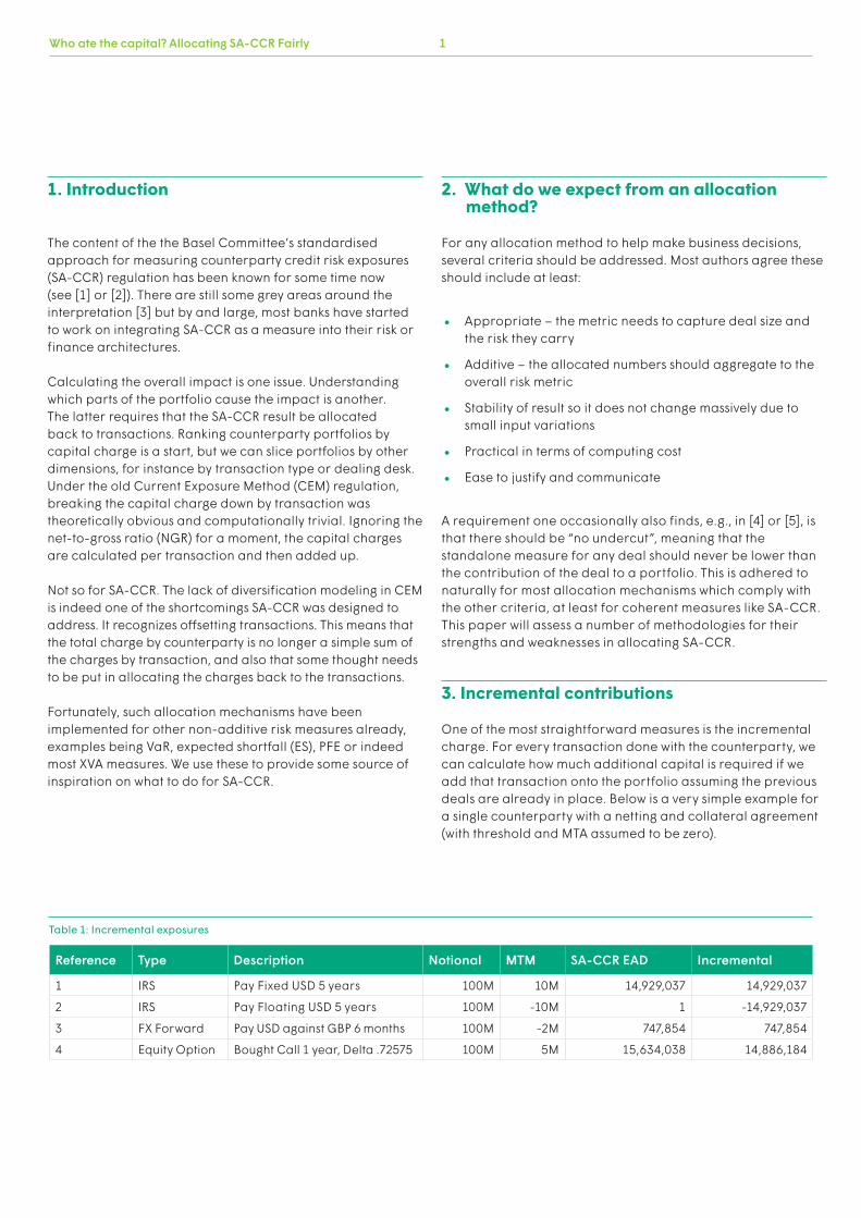
Reference Type Description Notional MTM SA-CCR EAD Incremental

1 IRS Pay Fixed USD 5 years 100M 10M 14,929,037 14,929,037

2 IRS Pay Floating USD 5 years 100M -10M 1 -14,929,037

3 FX Forward Pay USD against GBP 6 months 100M -2M 747,854 747,854

4 Equity Option Bought Call 1 year, Delta .72575 100M 5M 15,634,038 14,886,184

Table 1: Incremental exposures

2. What do we expect from an allocation method? For any allocation method to help make business decisions, several criteria should be addressed. Most authors agree these should include at least:

• Appropriate – the metric needs to capture deal size and the risk they carry

• Additive – the allocated numbers should aggregate to the overall risk metric

• Stability of result so it does not change massively due to small input variations

• Practical in terms of computing cost

• Ease to justify and communicate

A requirement one occasionally also finds, e.g., in [4] or [5], is that there should be “no undercut”, meaning that the standalone measure for any deal should never be lower than the contribution of the deal to a portfolio. This is adhered to naturally for most allocation mechanisms which comply with the other criteria, at least for coherent measures like SA-CCR. This paper will assess a number of methodologies for their strengths and weaknesses in allocating SA-CCR.

3. Incremental contributions One of the most straightforward measures is the incremental charge. For every transaction done with the counterparty, we can calculate how much additional capital is required if we add that transaction onto the portfolio assuming the previous deals are already in place. Below is a very simple example for a single counterparty with a netting and collateral agreement (with threshold and MTA assumed to be zero).

Who ate the capital? Allocating SA-CCR Fairly2

The example here is somewhat academic: the second transaction is just the mirror image of the first. But that drives the point home. In this order, transaction one gets a hefty risk charge and transaction two reduces it to zero again as it offsets it exactly. If, on the other hand, had they come in in reverse order, transaction two would have got a higher charge and transaction one would have receive all the credit for reducing it.

An incremental charge is still useful, it answers the question “If I have a given portfolio already and execute a new transaction now, by how much does it increase my capital charge?” But that if very different from having an established portfolio and then asking yourself which dealing desks cause which exposure. That answer should not depend on the order the transactions came in.

In fact, negative risk charges are impossible in this allocation mechanism. This means that no clear signal about risk reduction is ever sent. Shouldn’t a trader who helps reduce the risk get some benefit allocated to his trades? Jon Gregory in [6] (page 254) argues convincingly that he should, admittedly for CVA, not for SA-CCR, but the logic here is the same.

5. Euler allocation Euler allocation, sometimes called the gradient allocation, is a generic method originally developed for economic capital (EC) and later applied to CVA. It relies on calculating the increase in the chosen risk measure (in this case SA-CCR) due to an infinitesimal increase in the underlying position (in this case for each transaction). Details can be found in [7], [8] and [9]. In this instance the change in SA-CCR has been calculated by changing each position by one percent without changing the collateral already received.

This method is quite risk sensitive due to its design, but it is not naturally additive. So it is necessary to adjust the result in order to make it additive, pretty much in the same way as we did for the simple allocation mechanism in section 4.

4. Pro-rate allocation – the simplest of all allocation mechanisms For measures which are additive, such as the old CEM measure (ignoring the NGR ratio), or for that matter, for unnetted and uncollateralized SA-CCR exposure, the solution is trivial. One can just calculate the charge per transaction and the total is the portfolio charge.

Once a netting agreement is used, the portfolio charge is no longer the simple sum of the transactions and hence an allocation method of some sort is required. The simplest of all methods consist of calculating the standalone charge for each transaction, adding them up, working out what percentage each transaction contributes to that total and using it to allocate the portfolio charge back.

For such a simple mechanism this does not produce too bad a result. It is additive, relatively stable, easy to explain, and it reflects at least some of the risk. The latter is probably its biggest weakness: transaction two actually reduces the risk in this portfolio as it offsets transaction one. It does get a very low risk charge, but not a negative risk charge.

For our simple example portfolio this produces the following result:

Reference Type Description Standalone SA-CCR

Percentage of total

Allocated SA-CCR

1 IRS Pay Fixed USD 5 years 14,929,037 45.97% 7,186,505

2 IRS Pay Floating USD 5 years 46,768 0.14% 22,513

3 FX Forward Pay USD against GBP 6 months 747,854 2.30% 360,000

4 Equity Option Bought Call 1 year, Delta .72575 16,754,038 51.59% 8,065,020

Total 32,477,698 100.00% 15,634,038

Table 2: Simple allocation based on standalone charge


For our sample portfolio, this would be the result:

Table 3: Euler allocation

Reference Type Description Euler allocation

1 IRS Pay Fixed USD 5 years 13,343,222

2 IRS Pay Floating USD 5 years -11,682,520

3 FX Forward Pay USD against GBP 6 months -1,001,030

4 Equity Option Bought Call 1 year, Delta .72575 14,974,365

Total 15,634,038

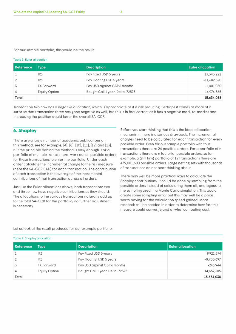
6. Shapley There are a large number of academic publications on this method, see for example, [4], [8], [10], [11], [12] and [13]. But the principle behind the method is easy enough. For a portfolio of multiple transactions, work out all possible orders for these transactions to enter the portfolio. Under each order calculate the incremental change to the risk measure (here the SA-CCR EAD) for each transaction. The contribution of each transaction is the average of the incremental contributions of that transaction across all orders. Just like the Euler allocations above, both transactions two and three now have negative contributions as they should. The allocations to the various transactions naturally add up to the total SA-CCR for the portfolio, no further adjustment is necessary. esult

Transaction two now has a negative allocation, which is appropriate as it is risk reducing. Perhaps it comes as more of a surprise that transaction three has gone negative as well, but this is in fact correct as it has a negative mark-to-market and increasing the position would lower the overall SA-CCR.

Let us look at the result produced for our example portfolio:

Table 4: Shapley allocation

Reference Type Description Euler allocation

1 IRS Pay Fixed USD 5 years 9,921,374

2 IRS Pay Floating USD 5 years -8,700,697

3 FX Forward Pay USD against GBP 6 months -243,944

4 Equity Option Bought Call 1 year, Delta .72575 14,657,305

Total 15,634,038

Before you start thinking that this is the ideal allocation mechanism, there is a serious drawback. The incremental charges need to be calculated for each transaction for every possible order. Even for our sample portfolio with four transactions there are 24 possible orders. For a portfolio of n transactions there are n factorial possible orders, so for example, a (still tiny) portfolio of 12 transactions there are 479,001,600 possible orders. Large netting sets with thousands of transactions do not bear thinking about.

There may well be more practical ways to calculate the Shapley contributions. It could be done by sampling from the possible orders instead of calculating them all, analogous to the sampling used in a Monte Carlo simulation. This would create some sampling error but this may well be a price worth paying for the calculation speed gained. More research will be needed in order to determine how fast this measure could converge and at what computing cost.


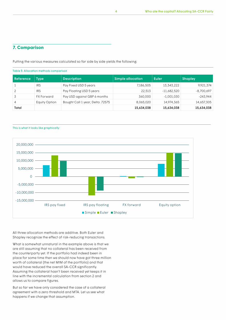
All three allocation methods are additive. Both Euler and Shapley recognize the effect of risk-reducing transactions.

What is somewhat unnatural in the example above is that we are still assuming that no collateral has been received from the counterparty yet. If the portfolio had indeed been in place for some time then we should now have got three million worth of collateral (the net MtM of the portfolio) and that would have reduced the overall SA-CCR significantly. Assuming the collateral hasn’t been received yet keeps it in line with the incremental calculation from section 2 and allows us to compare figures.

But so far we have only considered the case of a collateral agreement with a zero threshold and MTA. Let us see what happens if we change that assumption.

7. Comparison

Putting the various measures calculated so far side by side yields the following:

Reference Type Description Simple allocation Euler Shapley

1 IRS Pay Fixed USD 5 years 7,186,505 13,343,222 9,921,374

2 IRS Pay Floating USD 5 years 22,513 -11,682,520 -8,700,697

3 FX Forward Pay USD against GBP 6 months 360,000 -1,001,030 -243,944

4 Equity Option Bought Call 1 year, Delta .72575 8,065,020 14,974,365 14,657,305

Total 15,634,038 15,634,038 15,634,038

Table 5: Allocation methods comparison

This is what it looks like graphically:

-10,000,000

-15,000,000

-5,000,000

0

5,000,000

10,000,000

15,000,000

20,000,000

IRS pay fixed IRS pay floating FX forward Equity option

Simple Euler Shapley


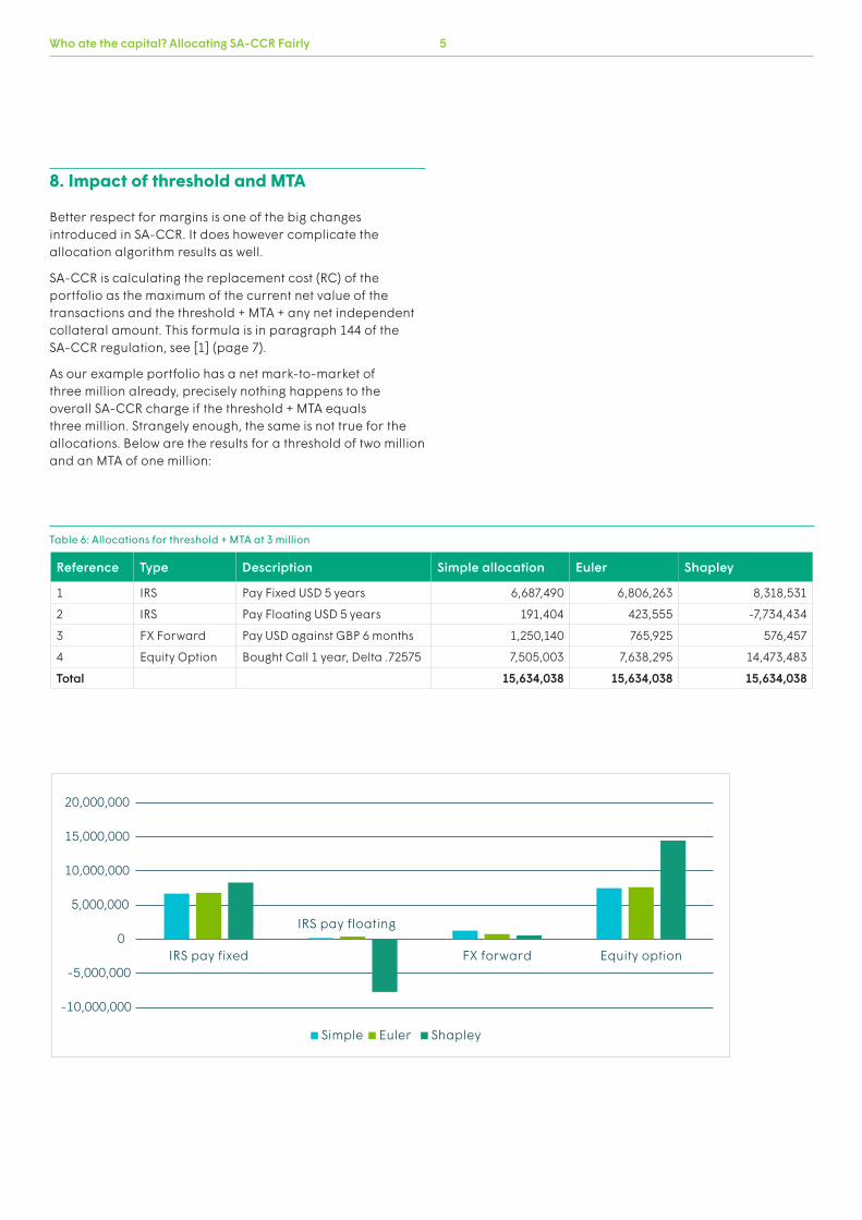
8. Impact of threshold and MTA Better respect for margins is one of the big changes introduced in SA-CCR. It does however complicate the allocation algorithm results as well.

SA-CCR is calculating the replacement cost (RC) of the portfolio as the maximum of the current net value of the transactions and the threshold + MTA + any net independent collateral amount. This formula is in paragraph 144 of the SA-CCR regulation, see [1] (page 7).

As our example portfolio has a net mark-to-market of three million already, precisely nothing happens to the overall SA-CCR charge if the threshold + MTA equals three million. Strangely enough, the same is not true for the allocations. Below are the results for a threshold of two million and an MTA of one million:



2 IRS Pay Floating USD 5 years 191,404 423,555 -7,734,434

3 FX Forward Pay USD against GBP 6 months 1,250,140 765,925 576,457


Total 15,634,038 15,634,038 15,634,038

Table 6: Allocations for threshold + MTA at 3 million

IRS pay floating

-10,000,000

-5,000,000

0

5,000,000

10,000,000

15,000,000

20,000,000

IRS pay fixed FX forward Equity option

ShapleyEulerSimple


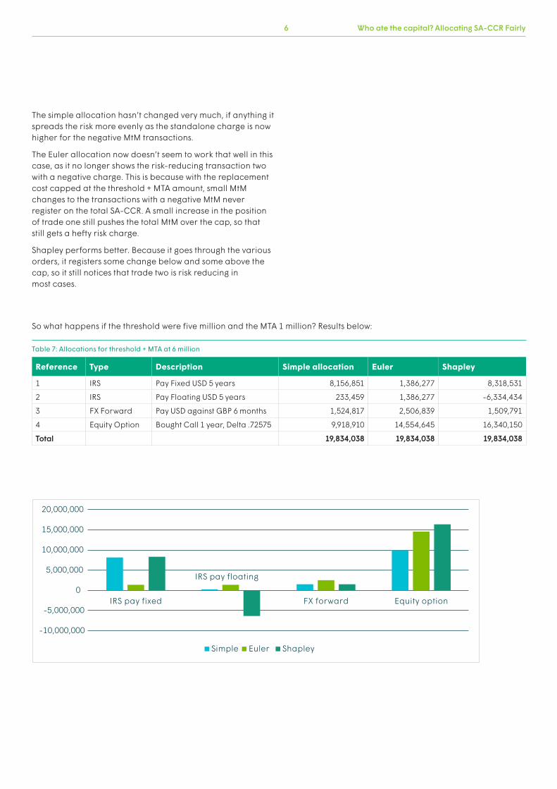
The simple allocation hasn’t changed very much, if anything it spreads the risk more evenly as the standalone charge is now higher for the negative MtM transactions.

The Euler allocation now doesn’t seem to work that well in this case, as it no longer shows the risk-reducing transaction two with a negative charge. This is because with the replacement cost capped at the threshold + MTA amount, small MtM changes to the transactions with a negative MtM never register on the total SA-CCR. A small increase in the position of trade one still pushes the total MtM over the cap, so that still gets a hefty risk charge.

Shapley performs better. Because it goes through the various orders, it registers some change below and some above the cap, so it still notices that trade two is risk reducing in most cases.



2 IRS Pay Floating USD 5 years 233,459 1,386,277 -6,334,434

3 FX Forward Pay USD against GBP 6 months 1,524,817 2,506,839 1,509,791


Total 19,834,038 19,834,038 19,834,038

So what happens if the threshold were five million and the MTA 1 million? Results below:

Table 7: Allocations for threshold + MTA at 6 million

IRS pay floating

Equity optionFX forwardIRS pay fixed

-10,000,000

-5,000,000

0

5,000,000

10,000,000

15,000,000

20,000,000



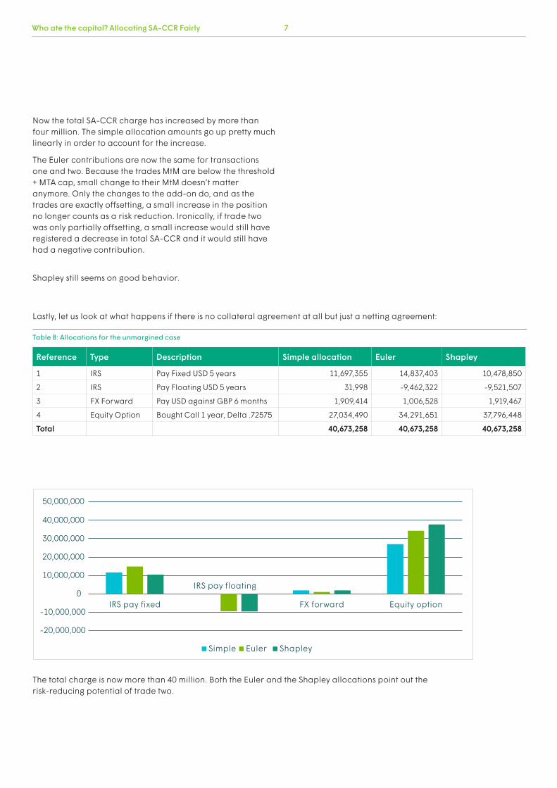
The total charge is now more than 40 million. Both the Euler and the Shapley allocations point out the risk-reducing potential of trade two.

Page 7

Equity optionFX forward

IRS pay floating


IRS pay fixed

-20,000,000

-10,000,000

0

10,000,000

20,000,000

30,000,000

40,000,000

50,000,000

Now the total SA-CCR charge has increased by more than four million. The simple allocation amounts go up pretty much linearly in order to account for the increase.

The Euler contributions are now the same for transactions one and two. Because the trades MtM are below the threshold + MTA cap, small change to their MtM doesn’t matter anymore. Only the changes to the add-on do, and as the trades are exactly offsetting, a small increase in the position no longer counts as a risk reduction. Ironically, if trade two was only partially offsetting, a small increase would still have registered a decrease in total SA-CCR and it would still have had a negative contribution.

Shapley still seems on good behavior.




3 FX Forward Pay USD against GBP 6 months 1,909,414 1,006,528 1,919,467


Total 40,673,258 40,673,258 40,673,258

Lastly, let us look at what happens if there is no collateral agreement at all but just a netting agreement:

Table 8: Allocations for the unmargined case


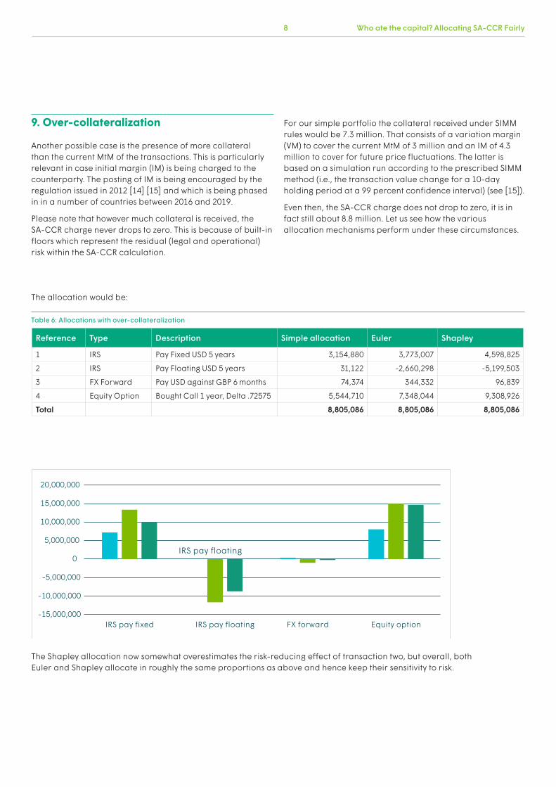
9. Over-collateralization Another possible case is the presence of more collateral than the current MtM of the transactions. This is particularly relevant in case initial margin (IM) is being charged to the counterparty. The posting of IM is being encouraged by the regulation issued in 2012 [14] [15] and which is being phased in in a number of countries between 2016 and 2019.

Please note that however much collateral is received, the SA-CCR charge never drops to zero. This is because of built-in floors which represent the residual (legal and operational) risk within the SA-CCR calculation.

For our simple portfolio the collateral received under SIMM rules would be 7.3 million. That consists of a variation margin (VM) to cover the current MtM of 3 million and an IM of 4.3 million to cover for future price fluctuations. The latter is based on a simulation run according to the prescribed SIMM method (i.e., the transaction value change for a 10-day holding period at a 99 percent confidence interval) (see [15]).

Even then, the SA-CCR charge does not drop to zero, it is in fact still about 8.8 million. Let us see how the various allocation mechanisms perform under these circumstances.




3 FX Forward Pay USD against GBP 6 months 74,374 344,332 96,839


Total 8,805,086 8,805,086 8,805,086

The allocation would be:

Table 6: Allocations with over-collateralization

The Shapley allocation now somewhat overestimates the risk-reducing effect of transaction two, but overall, both Euler and Shapley allocate in roughly the same proportions as above and hence keep their sensitivity to risk.

Page 5

-10,000,000

-15,000,000

-5,000,000

0

5,000,000

10,000,000

15,000,000

20,000,000

IRS pay fixed IRS pay floating FX forward Equity option



10. Conclusion The simple allocation does not recognise risk-reducing trades sufficiently, but otherwise, it is stable and by far the easiest to explain and justify. It is also quite easy to implement. For portfolios where risk-reducing trades are rare this is clearly a choice to be considered seriously.

For those who prefer a more sophisticated allocation method and wish to reward trades which actively reduce risk, both the Euler method and Shapley are worth considering, but each often produce results which are not easy to explain and hence they should be handled with care. Shapley is probably the most risk-sensitive methodology across the board. In all cases shown above, the Shapley contributions of trades one and two are almost opposite, which is correct given that they are each other’s mirror image.

Currently Shapley does have the additional disadvantage that it is prohibitively expensive to calculate for large netting sets. But, as alluded to in section 6 above, that problem may be solved at some point.

An additional issue to consider is how these methods perform for other risk metrics such as VaR, ES, EC, PFE or XVA measures. Using the same allocation method across the board has obvious advantages in terms of consistency of the methodology. This paper only looked at the allocation of SA-CCR.

11. Bibliography

1. Basel Committee on Banking Supervision (BCBS), The Standardised Approach for Measuring Counterparty Credit Exposures, 2014.

2. D. Karyampas and F. Anfuso, The SA-CCR for Counterparty Credit Risk Exposure - An Analysis From Risk and Pricing Perspectives, 2014.

3. Jean-Marc Schwob, SA-CCR – Not as Standard as You May Think, FIS Global, 2016.

4. M. Denault, Coherent Allocation of Risk Capital, Montreal: Ecole des H.E.C. (Montreal), 2001.

5. F. Sommerfeld, Capital Allocation (presentation), Towers Watson, 2013.

6. J. Gregory, Counterparty Credit Risk and Credit Value Adjustment, 2012.

7. D. Tasche, Capital Allocation to Business Units and Sub-portfolios: The Euler Principle, Lloyds TSB Bank, 2008.

8. M. El Gharib, A. Guenneugues, A. Leroy and G. Levavasseur, Optimal Allocation of the Diversification Capital, 2014.

9. M. Kalkbrener, An Axiomatic Approach to Capital Allocation, Mathematical Finance, (pages 425 – 437), 2005.

10. N. Tarashev, C. Borio and K. Tsatsaronis, The Systemic Importance of Financial Institutions, BIS Quaterly Review, No. 3 (pages 75 – 87), 2009.

11. E. Kromer and P. Cheridito, Ordered Contribution Allocations: Theoretical Properties and Applications, 2011.

12. T. S. Ferguson, Game Theory, Los Angeles: UCLA, 2014.

13. T. Boonen, A. De Waegenaere and H. Norde, A Generalization of the Aumann-Shapley Value for Risk Capital Allocation Problems, Tilburg University, Tilburg, 2012.

14. BCBS and IOSCO, Margin Requirements for Non-centrally Cleared Derivatives, 2013.

15. ISDA, ISDA – Standard Initial Margin Model for Non-cleared Dervivatives, 2013.


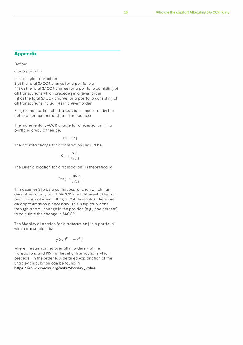
Appendix Define:

c as a portfolio

j as a single transaction S(c) the total SACCR charge for a portfolio c P(j) as the total SACCR charge for a portfolio consisting of all transactions which precede j in a given order I(j) as the total SACCR charge for a portfolio consisting of all transactions including j in a given order

Pos(j) is the position of a transaction j, measured by the notional (or number of shares for equities) The incremental SACCR charge for a transaction j in a portfolio c would then be: The pro rata charge for a transaction j would be:

I(j) P(j)

S(j)S(c)

i S(i)

The Euler allocation for a transaction j is theoretically:

This assumes S to be a continuous function which has derivatives at any point. SACCR is not differentiable in all points (e.g. not when hitting a CSA threshold). Therefore, an approximation is necessary. This is typically done through a small change in the position (e.g., one percent) to calculate the change in SACCR. The Shapley allocation for a transaction j in a portfolio with n transactions is: where the sum ranges over all n! orders R of the transactions and PR(j) is the set of transactions which precede j in the order R. A detailed explanation of the Shapley calculation can be found in https://en.wikipedia.org/wiki/Shapley_value

Pos(j)S(c)

Pos(j)

1! R(IR (j) PR (j))

322691

©2017 FISFIS and the FIS logo are trademarks or registered trademarks of FIS or its subsidiaries in the U.S. and/or other countries. Other parties’ marks are the property of their respective owners.

twitter.com/fisglobal

linkedin.com/company/fisglobal

www.fisglobal.com

[email protected]

About FISFISTM is a global leader in financial services technology, with a focus on retail and institutional banking, payments, asset and wealth management, risk and compliance, consulting and outsourcing solutions. Through the depth and breadth of our solutions portfolio, global capabilities and domain expertise, FIS serves more than 20,000 clients in over 130 countries. Headquartered in Jacksonville, Florida, FIS employs more than 55,000 people worldwide and holds leadership positions in payment processing, financial software and banking solutions. Providing software, services and outsourcing of the technology that empowers the financial world, FIS is a Fortune 500 company and is a member of Standard & Poor’s 500® Index. For more information about FIS, visit www.fisglobal.com

who ate the capital? allocating sa-ccr fairly · who ate the capital? allocating sa-ccr fairly 1 1....

Documents