Forschungsinstitut zur Zukunft der ArbeitInstitute for the Study of Labor

DI

SC

US

SI

ON

P

AP

ER

S

ER

IE

S

Where Did It Go Wrong?Marriage and Divorce in Malawi

IZA DP No. 9843

March 2016

Laurens CherchyeBram De RockSelma Telalagic WaltherFrederic Vermeulen

Where Did It Go Wrong? Marriage and Divorce in Malawi

Laurens Cherchye

CES, KU Leuven

Bram De Rock

ECARES, Université Libre de Bruxelles and KU Leuven

Selma Telalagic Walther Nuffield College, University of Oxford

Frederic Vermeulen

KU Leuven and IZA

Discussion Paper No. 9843 March 2016

IZA

P.O. Box 7240 53072 Bonn

Germany

Phone: +49-228-3894-0 Fax: +49-228-3894-180

E-mail: iza@iza.org

Any opinions expressed here are those of the author(s) and not those of IZA. Research published in this series may include views on policy, but the institute itself takes no institutional policy positions. The IZA research network is committed to the IZA Guiding Principles of Research Integrity. The Institute for the Study of Labor (IZA) in Bonn is a local and virtual international research center and a place of communication between science, politics and business. IZA is an independent nonprofit organization supported by Deutsche Post Foundation. The center is associated with the University of Bonn and offers a stimulating research environment through its international network, workshops and conferences, data service, project support, research visits and doctoral program. IZA engages in (i) original and internationally competitive research in all fields of labor economics, (ii) development of policy concepts, and (iii) dissemination of research results and concepts to the interested public. IZA Discussion Papers often represent preliminary work and are circulated to encourage discussion. Citation of such a paper should account for its provisional character. A revised version may be available directly from the author.

IZA Discussion Paper No. 9843 March 2016

ABSTRACT

Where Did It Go Wrong? Marriage and Divorce in Malawi* Do individuals divorce for economic reasons? Can we measure the attractiveness of new matches in the marriage market? We answer these questions using a structural model of the household and a rich panel dataset from Malawi. We propose a model of the household with consumption, production and revealed preference conditions for stability on the marriage market. We define marital instability in terms of the consumption gains to remarrying another individual in the same marriage market, and to being single. We find that a 1 percentage point increase in the wife’s estimated consumption gains from remarriage is significantly associated with a 0:6 percentage point increase in divorce probability in the next three years. In a multinomial model, higher values of consumption gains from remarriage raise the odds of divorce and remarriage but not of divorce and singleness. These findings provide out-of-sample validation of the structural model and shed new light on the economic determinants of divorce. JEL Classification: D11, D12, D13, J12 Keywords: marriage market, divorce, Malawi, agricultural production, revealed preference Corresponding author: Frederic Vermeulen Department of Economics University of Leuven (KU Leuven) Naamsestraat 69 3000 Leuven Belgium E-mail: frederic.vermeulen@kuleuven.be

* We thank seminar participants at University College London for useful discussion. Laurens Cherchye gratefully acknowledges the European Research Council (ERC) for his Consolidator Grant 614221. Part of this research is also funded by the FWO (Research Fund-Flanders). Bram De Rock gratefully acknowledges FWO and BELSPO for their financial support. Frederic Vermeulen gratefully acknowledges financial support from the Research Fund KU Leuven through the grant STRT/12/001 and from the FWO through the grant G057314N.

1 Introduction

Becker (1973, 1974) convincingly argued that the institution of marriage can be analyzed by means

of modern microeconomic theory. In his ground-breaking work, as well as in subsequent work by

Becker, Landes and Michael (1977), the concept of the marriage market is introduced, which rests

on the simple but powerful assumption that individuals are rational utility maximizers who compete

as they seek mates. Such a framework implies that each individual looks for the best mate subject

to the restrictions imposed by the marriage market. An important concept in this theory is gains

to marriage, which depend on the particular union as well as on the opportunities implied by the

marriage market as a whole.

The gains to marriage do not only consist of companionship and the production and rearing

of children. There are also considerable economic gains, such as the sharing of public goods or

the division of labour within unions (see Browning, Chiappori and Weiss, 2014, for an extensive

discussion). The economic gains to marriage play a crucial role in the recent model proposed by

Cherchye, Demuynck, De Rock and Vermeulen (2015) to analyze the impact of the marriage market

on the intrahousehold distribution of resources. In their model, the collective model (Chiappori,

1988, 1992) is combined with the assumption of a stable marriage market, a concept that is directly

related to the ideas in Becker (1973, 1974) and Becker, Landes and Michael (1977). The model

predicts that the more attractive the outside options of a spouse, the higher is his or her share of

the household�s resources. These outside options improve with one�s productivity, which implies

that the marriage market can explain the widely observed positive relationship between wages and

the share of household resources consumed (see, e.g., Blundell, Chiappori, Magnac and Meghir,

2007, Cherchye, De Rock and Vermeulen, 2012, and Cherchye, De Rock, Lewbel and Vermeulen,

2015).

In this paper, we argue that the economic aspects of marriage and divorce may be even more

salient in developing countries. As a consequence, we focus on the estimation of the gains to

marriage and divorce in Malawi, which is one of the poorest countries in the world. Given the

importance of agricultural production in this setting, we extend the theoretical model in Cherchye,

Demuynck, De Rock and Vermulen (2015) to include production. Appealingly, we can do this while

allowing for both heterogeneous individual preferences and household production technologies. We

estimate this model on panel data drawn from the Malawi Integrated Household Survey (IHS),

and we test whether model-based measures of marital instability predict future divorces. As we

discuss in more detail in Section 3.1, Malawi is an attractive setting for the estimation of this model

because it has one of the highest divorce rates in Africa.1 Reniers (2003) shows that in Malawi

lifetime divorce probabilities are between 40% and 65%. He also shows that remarriage is almost

universal: within two years of divorce, over 40% of women have remarried in the sample, and this

�gure reaches almost 90% after ten years. Thus, divorce and remarriage is a realistic outside option

1Moreover, Dunbar, Lewbel and Pendakur (2013) also used the collective model to study the consumption behav-iour of Malawian households. These authors particularly focused on identifying resource shares of children. In thecurrent study, we follow a similar collective approach to analyze marriage stability.

2

for married individuals.

Our model yields two structural indices for marriage instability: the �rst index captures how

much better o¤ (in consumption terms) the individual would be if single (the Individual Rationality

(IR) index), while the second index measures how much better o¤ the individual would be if (s)he

remarried another individual in the same marriage market (the Blocking Pair (BP) index). In the

empirical analysis, we compute these instability indices for each married individual in the 2010

wave of our data. We then link these measures of instability to observed divorces between the 2010

and 2013 waves of the IHS. This sheds light on the importance of economic gains to marriage and

divorce and how well our model is able to predict divorces and subsequent remarriages.

Our empirical results demonstrate that the wife�s BP index signi�cantly predicts divorce in the

panel. A one-percentage-point increase in the wife�s BP index, as a proportion of her household�s

income, raises the probability of divorce by 0:6 percentage points on average. This is a non-

negligible e¤ect, as the proportions of currently divorced and married individuals in the population

suggest an annual divorce probability of 8:5%.2 Therefore, we �nd that a model-based predictor

of divorce correlates with out-of-sample realizations of divorce, hence validating the structural

model. Interestingly, this signi�cant association cannot be explained by spouses�wages, land income

or nonlabour income which, alongside intrahousehold sharing, are the key determinants of the

BP index in the structural model. This suggests that intrahousehold sharing e¤ectively plays

an important role in the gains to marriage and divorce. As an extension to these results, we also

estimate a multinomial model that di¤erentiates between individuals who divorce and remain single,

and those who divorce and remarry. Interestingly, we �nd that the wife�s BP index is signi�cantly

associated with the wife divorcing and remarrying, but not divorcing and remaining single. This is

consistent with the idea that the BP index captures the attractiveness of remarriage.

Our paper makes two contributions to the literature. First, from a methodological point of

view, it extends the model of Cherchye, Demuynck, De Rock and Vermeulen (2015) to account

for domestic production in modeling households�economic behavior. This is particularly relevant

for households in developing countries, for which agricultural production activities are prevalent.

Interestingly, this also allows us to estimate shadow wages and land prices, which are often missing

or su¤er from measurement error in empirical applications. A distinguishing feature of our method

is that it belongs to a revealed preference tradition that is free of any parametric assumptions, and

thus obtains robust conclusions. See Samuelson (1938), Afriat (1967), Diewert (1973) and Varian

(1982) for early contributions on revealed preference analysis of household consumption behavior.

More recently, Cherchye, De Rock and Vermeulen (2007, 2009, 2011) have extended this seminal

work towards the analysis of collective households.

Second, our empirical application o¤ers a novel perspective on the growing literature on the

economic drivers of divorce. This literature has focused on the relationship between economic

shocks and divorce. For example, Weiss and Willis (1997) �nd that shocks to husbands�earning

2Assuming individuals change from marriage to divorce states according to a Markov process, using the proportionsof individuals currently married and divorced in the IHS and using the remarriage probabilities in Reniers (2003),implies an annual divorce probability of 8:5%.

3

capacity reduce the probability of divorce, while shocks to wives�earning capacity increase it. In

a similar vein, Boheim and Ermisch (2001) �nd that positive economic surprises among British

households reduce the probability of union dissolution. Charles and Stephens (2004) compare the

e¤ect of spousal job loss and spousal disability, and �nd that job loss raises the probability of divorce

but disability does not. Other papers examine the e¤ect of lottery winnings on divorce (Hankins

and Hoekstra, 2011) and the relationship between house prices and divorce (Farnham, Schmidt

and Sevak, 2011). An alternative way to model observed patterns of cohabitation, marriage and

divorce is proposed by Brien, Lillard and Stern (2006), who model match quality as an experience

good, à la Jovanovic�s (1979) labour market matching model. Overall, the evidence suggests that

there is an important economic component to divorce, although these studies do not consider

the potential for remarriage, and except for Brien, Lillard and Stern (2006), do not implement a

structural measure of the economic gains to divorce. As explained above, our structural approach

combines the collective consumption model with the assumption of marriage stability, which allows

us to explicitly incorporate the importance of intrahousehold sharing and options on the marriage

market in the analysis of marriage and divorce decisions.

The rest of this paper unfolds as follows. Section 2 introduces our revealed preference method-

ology for analysing stability of marriage. Here, we also de�ne our IR and BP indices for marriage

stability. In Section 3 we provide further motivation for our empirical research question by explain-

ing the speci�c setting of Malawi. We also present our sample of households and the construction of

the marriage markets used in our empirical application. Section 4 presents some summary statistics

on the main outcomes of our structural model. These results will motivate our regression analyses

in Section 5, in which we focus on the relationship between the economic gains to divorce (captured

by our IR and BP indices) and divorce and remarriage probabilities. Section 6 concludes. The

Appendix gives additional details on our data construction method.

2 Consumption, production and marriage stability

Our method for measuring instability of marriage builds on a recent paper by Cherchye, Demuynck,

De Rock and Vermeulen (2015). These authors de�ned a revealed preference characterization of

household consumption under stable marriage to analyze the intrahousehold allocation of resources.

A novel feature of our analysis is that we integrate agricultural production in this revealed preference

framework, thus linking productivity to marriage decisions. As we will explain further on (in Section

3.1), agricultural production is an important dimension of household decision behavior in Malawi.

It is the primary source of livelihood and a crucial determinant of outside options. Moreover, our

structural modeling of household production allows us to use shadow wages and land prices in our

analysis of marriage stability. This is particularly convenient in view of our empirical application,

because fully reliable wage and land price information is not available for the Malawian households

that we study. As this last feature is often characteristic to data sets on developing countries, this

also indicates the usefulness of our model in other application settings.

4

2.1 Notation and components of the structural model

We focus on the marriage stability of couples that consist of a female a and a male b. In what

follows, we will often refer to individual i = a; b. Let A be a �nite set of females and B a �nite set

of males. The marriage market is de�ned by a matching function � : A[B ! A[B. This functionsatis�es, for all a 2 A and b 2 B,

� (a) 2 B; � (b) 2 A;

� (a) = b 2 B if and only if � (b) = a 2 A:

In words, the function � assigns to every female or male a partner of the other gender (i.e. � (a) = b

and � (b) = a). In this methodological section we will assume that jAj = jBj, which means thatall individuals are matched. In contrast, in the empirical part of this paper we will account for

the possibility that jAj 6= jBj and that a married individual may consider remarrying a single ofthe other gender. Actually, if we do not include rationalizability conditions for singles�behavior,

it is relatively straightforward to formally include this possibility in the models below.3 However,

unless there is a shortage on one side of the marriage market, rationalizing the behavior of singles

requires an explicit model for frictions on the marriage market and/or marriage costs. To focus our

discussion, we abstract from such extensions in the current study.

Each individual i is assumed to spend her or his total time endowment (denoted by T i 2 R+) onleisure (li 2 R+), market work (mi 2 R+) and agricultural work on the household�s land (denotedby hi 2 R+). The individual time budget constraint thus equals:

T i = mi + hi + li:

The price of time is individual i�s wage, which we represent by wi 2 R++:To model agricultural production, we assume that there are three types of inputs: the individ-

uals�time spent on agricultural labour (ha and hb), land (L 2 R+) and other input (x 2 R+; e.g.fertilizer). We distinguish between land of the female (La 2 R+), land of the male (Lb 2 R+) andjoint �household�land (L(a;b) 2 R+), i.e.

L = La + Lb + L(a;b):

For a given match (a; b), we assume a common price for the three land types, i.e. the price of La,

Lb and L(a;b) is given by z(a;b) 2 R++. Other input x is assumed to be a Hicksian aggregate with aprice that is normalized to unity. The inputs are transformed into an output y 2 R+ by means ofan agricultural production function F

�ha; h�(a); L; x

�. We assume that this function is increasing

in its arguments and characterized by constant returns to scale (in line with Pollak and Wachter,

3Speci�cally, some of the variables in Propositions 1 and 2 (individual quantities, personalized prices, share ofnon-labour income and shadow wages) must be set equal to zero in the case of singles. But the basic structure of therationalizability conditions in the propositions remains intact.

5

1975). The output associated with agricultural production is again a Hicksian aggregate, with a

price that is normalized at unity. The household is further associated with a nonlabour income

n(a;b) 2 R+.The total income of a household consists of income from market work, agricultural production

and nonlabour income. It is allocated to a Hicksian aggregate good with a price that is normalized

to unity. This Hicksian aggregate is used for the private consumption of both spouses (denoted

by qa and qb 2 R+) and the household�s expenditures on a public good (denoted by Q 2 R+).Examples of private goods are expenditures on food and clothing, while an example of a public

good is expenditure on children.

Finally, each individual i is assumed to derive utility from leisure, private consumption as

well as public consumption. The preferences of individual i are represented by a utility function

U i�li,qi; Q

�that is assumed to be continuous, concave and strictly increasing in leisure li and

private consumption qi, and increasing in public consumption Q.

2.2 Marriage stability: theoretical characterization

Let us now de�ne a stable marriage allocation. We will say that an allocation is stable if it satis�es

three equilibrium conditions.

First, at the consumption level, we adopt the collective approach of Chiappori (1988, 1992)

and assume that within-household allocations are Pareto e¢ cient. Formally, this means that every

matched couple (a; � (a)) chooses a consumption allocation that solves

maxla;l�(a);qa;q�(a);Q

Ua (la; qa; Q) + �U�(a)

�l�(a); q�(a); Q

�(1)

s.t.

wala + w�(a)l�(a) + qa + q�(a) +Q � N + waT a + w�(a)T �(a);

where � represents the Pareto weight of male � (a) relative to female a, and N = n+ x+ zL. We

note that the Pareto weights are in general not constant. They will vary with factors such as wages.

Next, we remark that N contains nonlabour income n as well as the rental value of land (quantities

La, Lb and L(a;b), which are evaluated at the prices z(a;b) for each match (a; b)) and the cost for

the other input x. In terms of the household�s budget equation in (1), note that the total private

consumption on the left-hand side of the budget equation contains both market consumption and

agricultural output. Therefore we need to add the cost needed to produce this output to the right-

hand side as well. These expenditures are, of course, equal to the expenses on the inputs needed to

produce the speci�c output. The optimal composition of the inputs and the size of the agricultural

output is determined next.

Second, at the production level, we follow the set-up of Chiappori (1997) and assume that each

6

household (a; � (a)) is a pro�t maximizer, i.e. the chosen output-input combination solves

maxha;h�(a);L;x

y � waha � w�(a)h�(a) � zL� x (2)

s.t.

y = F�ha; h�(a); L; x

�:

Third, we assume that the marriage market is stable. Using the de�nition of Gale and Shapley

(1962), marriage stability imposes that marriage matchings satisfy the conditions of Individual

Rationality and No Blocking Pair. To formalize the notion of Individual Rationality, we let UaH and

U bH represent female a�s and male b�s utility in their given marriage. Then, Individual Rationality

requires

UaH � UaS and U bH � U bS ; (3)

where UaS and UbS denote the female�s and male�s maximum attainable utilities as singles, respec-

tively. Intuitively, Individual Rationality imposes that no female or male wants to exit the marriage

and become single.

Next, to formalize the condition of No Blocking Pair, we let UaP(a;b) and UbP(a;b)

represent any

possible realization of utilities for female a and male b if they formed a pair. Then, the No Blocking

Pair requirement imposes that

U iP(a;b) > UiH implies U

i0H > U

i0P(a;b)

for i; i0 2 fa; bg; i 6= i0: (4)

In words, a marriage allocation has no blocking pairs if no female a and male b are both better o¤,

with at least one individual strictly better o¤, by remarrying each other instead of staying with

their current partner.

In what follows, we will quantify deviations from the Individual Rationality and No Blocking

Pair conditions by Individual Rationality (IR) and Blocking Pair (BP) indices, which measure the

degree of marriage instability. We will compute these indices under the maintained assumptions

that intrahousehold consumption allocations are Pareto e¢ cient and production allocations are

pro�t e¢ cient.

2.3 Marriage stability: empirical conditions

For a given marriage market, the data set D contains the following information:

� matching function �,

� time uses li, mi and hi (and time endowment T i) of each individual i,

� wage wi of each individual i,

� consumption quantities (q(a;�(a)); Q(a;�(a))) of every matched couple (a; �(a)),

7

� land quantities La, L�(a) and L(a;�(a)) of every matched couple (a; �(a)),

� land price z(a;�(a)) of every matched couple (a; �(a)),

� input quantity x(a;�(a)) of every matched couple (a; �(a)),

� output quantity y(a;�(a)) of every matched couple (a; �(a)),

� nonlabour income n(a;�(a)) of every matched couple (a; �(a)).

As is standardly assumed for household data, we remark that the set D does not include

information on individuals�private consumption; only the aggregate household quantities q(a;�(a))

are observed. The individuals� private quantities will be treated as unknowns in our empirical

conditions for marriage stability.4 Next, in what follows we will assume that wages and land prices

remain the same when individuals exit marriage (and become single or remarry), i.e. divorce has

no productivity e¤ects. For the moment, we assume that these prices and wages are perfectly

observed. We will relax this assumption later on (see Section 2.4).

Characterizing stable marriage As explained in Section 2.2, we say that the data set D is

consistent with a stable matching if it allows the speci�cation of individual utility functions Ua

and U b that represent the observed consumption behavior as Pareto e¢ cient and the observed

marriages as stable. We use revealed preference conditions that are intrinsically nonparametric, in

the sense that they do not require an explicit (parametric) speci�cation of the functions Ua and

U b: In particular, based on Cherchye, Demuynck, De Rock and Vermeulen (2015, Proposition 2),

we obtain the following characterization of a stable marriage matching.5

Proposition 1 The data set D is consistent with stable matching � only if there exist,

a. for each matched pair (a; �(a)) (a 2 A), individual quantities q(a;�(a))a ; q(a;�(a))�(a) 2 R+ and

nonlabour incomes Na; N�(a) 2 R+ that satisfy

q(a;�(a))a + q(a;�(a))�(a) = q(a;�(a));

Na +N�(a) = n(a;�(a)) + x(a;�(a)) + z(a;�(a))L(a;�(a));

b. and, for each pair (a; b) (a 2 A, b 2 B), personalized prices P (a;b)a , P (a;b)b 2 R+ that satisfy

P (a;b)a + P(a;b)b = 1;

4 In our empirical application, part of the private consumption will be assignable to men and women (i.e. individualexpenditures on health, education and clothing; see the Appendix). Such information is easy to include in the linearconditions in Proposition 1. Basically, it implies lower bound restrictions on the unknowns q(a;�(a))a and q(a;�(a))�(a) . Forease of notation, we will not explicitly consider this re�nement here.

5After suitably adapting the notation of Cherchye, Demuynck, De Rock and Vermeulen (2015), the proof ofProposition 1 proceeds similarly as the proof of these authors�Proposition 2. Given this analogy, and for compactness,we do not explicitly include a formal proof in the current paper. Evidently, the proof can be obtained upon request.

8

such that the following constraints are met:

i. individual rationality restrictions for all females a 2 A and males b 2 B, i.e.

Na + z(a;�(a))La + waT a � wala + q(a;�(a))a +Q(a;�(a)), (5)

N b + z(�(b);b)Lb + wbT b � wblb + q(�(b);b)b +Q(�(b);b),

ii. no blocking pair restrictions for all a 2 A and b 2 B, i.e.�Na + z(a;�(a))La + waT a

�+�N b + z(�(b);b)Lb + wbT b

�(6)

��wala + wblb

�+�q(a;�(a))a + q

(�(b);b)b

�+�P (a;b)a Q(a;�(a)) + P

(a;b)b Q(�(b);b)

�:

Thus, consistency of D with a stable matching requires that it is possible to specify individual

quantities q(a;�(a))a ; q(a;�(a))�(a) and personalized prices P (a;b)a , P (a;b)b that satisfy a set of constraints that

are linear in these unknown quantities and prices. Therefore a convenient feature of the conditions

in Proposition 1 is that they can be checked through simple linear programming, which means that

they are easy to apply in practice. Also note that the observability of individual land constitutes

a natural lower bound in conditions (5) and (6).

We refer to Cherchye, Demuynck, De Rock and Vermeulen (2015) for a detailed explanation

of Proposition 1. Here, we highlight the �revealed preference� interpretation of the conditions (i)

and (ii) in terms of stable marriage allocation. First, the inequalities (5) in condition (i) require,

for each individual male and female, that the budget conditions under single status (with income

Na + z(a;�(a))La + waT a for female a and N b + z(�(b);b)Lb + wbT b for male b) do not allow buying

a bundle that is strictly more expensive than the one consumed under the current marriage (i.e.�la; q

(a;�(a))a ; Q(a;�(a))

�for female a and

�lb; q

(�(b);b)b ; Q(�(b);b)

�for male b). Indeed, if this condition

is not met, then at least one man or woman is better o¤ (i.e. can attain a strictly better bundle)

as a single, which means that the marriage allocation is not stable.

In a similar vein, the right hand side of the inequality (6) in condition (ii) gives the sum value

of the bundles within marriage for female a (i.e. wala+ q(a;�(a))a + P

(a;b)a Q(a;�(a))) and male b (i.e.

wblb + q(�(b);b)b + P

(a;b)b Q(�(b);b)), evaluated at the prices that pertain to the pair (a; b) (and using

the personalized prices P (a;b)a and P (a;b)b to evaluate the public quantities). The inequality then

requires that the pair�s total income (i.e. Na + z(a;�(a))La +waT a +N b + z(�(b);b)Lb +wbT b) must

not exceed this sum value. Intuitively, if this condition is not met, then woman a and man b can

allocate their income so that both of them are better o¤ (with at least one strictly better o¤) than

with their current matches �(a) and �(b), which makes (a; b) a blocking pair.

Quantifying marriage instability An important focus of our empirical analysis will be on

marriage instability. As explained before, we quantify marital instability in terms of individuals�

9

consumption gains from divorcing and remaining single or remarrying. More speci�cally, we use

our model to de�ne two structural measures of instability: our Individual Rationality (IR) indices

capture how much better o¤ (in consumption terms) individuals would be as a single person, and

our Blocking Pair (BP) indices measure how much better o¤ individuals would be when remarrying

other partners in the same marriage market.

To operationalize these ideas, for each exit option from marriage (i.e. become single or remarry

another potential partner), we quantify the minimal within-marriage consumption increase that

is needed to represent the observed marriage as stable with respect to the given exit option (as

characterized by the conditions (i) and (ii) in Proposition 1). This indicates how far the observed

behavior (with the original income levels) is from stable behavior. Conversely, it measures the

possible gain from divorce when choosing a particular exit option and, therefore, we can interpret

it as revealing the degree of marriage instability.

Formally, starting from our characterization in Proposition 1, we include an instability index

in each restriction of individual rationality (sIRa;; for the female a and sIR;;b for the male b) and no

blocking pair (sBPa;b for the pair (a; b)). We replace the inequalities in (5) by�Na + z(a;�(a))La + waT a

�� sIRa;; � w

ala + q(a;�(a))a +Q(a;�(a)), (7)�N b + z(�(b);b)Lb + wbT b

�� sIR;;b � w

blb + q(�(b);b)b +Q(�(b);b),

and the inequality (6) by�Na + z(a;�(a))La + waT a

�+�N b + z(�(b);b)Lb + wbT b

�� sBPa;b (8)

��wala + wblb

�+�q(a;�(a))a + q

(�(b);b)b

�+�P (a;b)a Q(a;�(a)) + P

(a;b)b Q(�(b);b)

�,

and we add the restriction 0 � sIRa;;; sIR;;b ; s

BPa;b . The indices s

IRa;;, s

IR;;b and s

BPa;b represent individuals�

consumption gains when choosing particular exit options from marriage: sIRa;; when female a

becomes single, sIR;;b when male b becomes single, and sBPa;b when a and b remarry with each other.

Clearly, imposing sIRa;;; sIR;;b ; s

BPa;b = 0 obtains the original (sharp) conditions in Proposition 1, while

higher values for sIRa;;, sIR;;b and s

BPa;b correspond to larger deviations from stable marriage behavior.

In our application, we measure the degree of instability of our data set by computing

minsIRa;;;s

IR;;b;s

NBPa;b

Xa

sIRa;; +Xb

sIR;;b +Xa

Xb

sBPa;b ; (9)

subject to the feasibility constraints (a) and (b) in Proposition 1 and the linear constraints (7) and

(8). By solving (9), we compute IR indices for the individual rationality constraints (sIRa;; and sIR;;b

in (7)) and BP indices for the no blocking pair constraints (sBPm;w in (8)). Correspondingly, for

each exit option, we can de�ne an associated gain from divorce. In our application, we will de�ne

10

�relative�divorce gains by setting out these gains as proportions of the household�s income:

2.4 Shadow wages and land prices

So far we have assumed that prices are observed. If prices are not observed, we can use shadow

prices. To do so, we can use the structural model that we de�ned in Section 2.2, which assumes

pro�t e¢ cient behavior under constant returns to scale (see (2)). In the spirit of Proposition 1, we

use a characterization of pro�t e¢ ciency that is nonparametric, which here means that it does not

require an explicit speci�cation of the production technology (represented by the function F ).6

Let the true wages (wi for each individual i = a; b) and land prices (z(a;�(a)) for each matched

pair (a; �(a))) be unobserved. Then, we can de�ne shadow wages and prices under the identifying

assumption of pro�t e¢ cient production behavior. Speci�cally, we say that the data set D is

consistent with shadow pro�t maximization if we can specify a production function F such that

pro�t e¢ ciency of the observed production behavior is supported by shadow prices. Adapting the

notation in Varian (1984, Theorem 6) to our setting, we obtain the following characterization of

productive e¢ cient behavior.

Proposition 2 The data set D is consistent with shadow pro�t maximization if and only if,for each matched pair (a; �(a)) (a 2 A), there exist shadow wages wa; w�(a) 2 R+ and a land pricez(a;�(a)) 2 R+ that satisfy

0 = y(a;�(a))� (10)hwaha + w�(a)h�(a) + z(a;�(a))

�La + L�(a) + L(a;�(a))

�+ x(a;�(a))

isuch that, for all a0 2 A,

0 � y(a0;�(a0))� (11)hwaha

0+ w�(a)h�(a

0) + z(a;�(a))�La

0+ L�(a

0) + L(a0;�(a0))

�+ x(a

0;�(a0))i:

Basically, the conditions (10) and (11) require that there exist shadow prices such that the

observed input-output combination of each matched pair (a; �(a)) achieves a pro�t of zero (see

(10)), which must exceed the pro�t for any household (a0; �(a0)) (with a0 2 A) under the sameprices (see (11)): This condition of zero maximum pro�t directly follows from our constant returns

to scale assumption. We append these pro�t e¢ ciency restrictions to the stability conditions above.

As a result, our marriage stability analysis will use shadow wages and land prices that are identi�ed

under the assumption of e¢ cient household production. See also the linear program that we present

below (in (14)).

Our empirical analysis will make use of two extensions of the characterization in Proposition

2. First, the characterization only imposes that shadow prices should be non-negative. Obviously,

6See, for example, Afriat (1972) and Varian (1984) for seminal contributions on this nonparametric approach toanalyzing e¢ cient production behaviour.

11

this allows for shadow prices that are unrealistic proxies of the true (unobserved) prices (e.g. prices

that are in�nitely high). To exclude such unrealistic scenarios, we impose lower and upper bounds

on possible prices. Speci�cally, we append the restrictions

wa � wa � wa, wb � wb � wb and z(a;�(a)) � z(a;�(a)) � z(a;�(a));

for wa, wb, z(a;�(a)) 2 R++ and wa, wb, z(a;�(a)) 2 R++ prede�ned lower and upper bounds. TheAppendix explains how we de�ne these bounds in our empirical application.

Our second extension pertains to the fact that the characterization in Proposition 2 implic-

itly assumes that di¤erent households are characterized by homogeneous production technologies.

Clearly, in practice we need to account for unobserved technological heterogeneity across house-

holds, i.e. some households have access to less e¢ cient production technologies than others. To

account for this heterogeneity, we introduce deviational variables �a+, �a�, �a;a0 2 R+ for each

matched pair (a; � (a)). These variables capture possible deviations from the original (sharp) con-

ditions in Proposition 2, which can thus be explained by heterogeneous technologies characterizing

the di¤erent production processes.7

Formally, in our pro�t e¢ ciency characterization in Proposition 2, we replace the equality

restriction (10) by

�a+ � �a� = y(a;�(a))� (12)hwaha + w�(a)h�(a) + z(a;�(a))

�La + L�(a) + L(a;�(a))

�+ x(a;�(a))

i;

and the inequality restriction (11) by

�a;a0 � y(a0;�(a0))� (13)h

waha0+ w�(a)h�(a

0) + z(a;�(a))�La

0+ L�(a

0) + L(a0;�(a0))

�+ x(a

0;�(a0))i:

Basically, the variables �a+, �a�, �a;a0account for deviations from the zero maximum pro�t that

appears at the left hand side in the original conditions (10) and (11), i.e. they capture deviations

from the assumption of productive e¢ ciency under constant returns to scale with homogeneous

household technologies.

In our application, we use shadow prices that minimize the aggregate value of the deviational

variables,Pa

��a+ + �a� +

Pa0 �

a;a0�. In combination with the objective (9) de�ned above, this

7Deviational variables are also used in the �goal programming�approach to deal with infeasible linear programs.

12

obtains (with 0 � � � 1)

minsIRa;;;s

IR;;b;s

NBPa;b ;�a+;�a�;�a;a0

�

Xa

sIRa;; +Xb

sIR;;b +Xa

Xb

sBPa;b

!(14)

+(1� �) X

a

�a+ + �a� +

Xa0

�a;a0

!!;

subject to the constraints (a) and (b) in Proposition 1, the stability constraints (7) and (8) and the

pro�t e¢ ciency constraints (12) and (13). Because all constraints are linear in unknowns, we can

compute the solution values of sIRa;;, sIR;;b , s

BPa;b , �

a+, �a� and �a;a0by simple linear programming.

In (14), the parameter � is a tuning parameter that represents the �penalization�weight of

the marriage instability indices relative to the technological heterogeneity variables. As we use

pro�t e¢ ciency as our identifying assumption for the shadow wages and land prices, we set � very

small. This can be interpreted in terms of a two-stage optimization process: in the �rst stage, we

de�ne shadow prices as the prices that correspond to minimal deviations from our pro�t ine¢ ciency

conditions (measured byPa

��a+ + �a� +

Pa0 �

a;a0�); in the second stage, we compute instability

indices for the given shadow prices (by minimizingPa sIRa;;+

Pb sIR;;b+

Pa

Pb sBPa;b ).

3 Malawian households: setting, data and marriage markets

We start by sketching the speci�c context of Malawi. This will show that this country provides

an interesting setting to investigate our question regarding the impact of economic determinants

on marriage and divorce decisions. In a following step, we discuss our data selection and the

construction of households�marriage markets.

3.1 The Malawi setting

Malawi is a poor country in Sub-Saharan Africa. The GDP per capita was $226 in 2013 (World

Bank). It ranks 174th out of 187 countries on the 2014 Human Development Index, with a life

expectancy of 55.3 years at birth. This is partly due to the prevalence of HIV, which is one of the

highest in the world at 10% in 2014 (World Bank). Malawi ranked 129th out of 140 countries on the

Gender Inequality Index, which measures inequality along three dimensions: reproductive health,

empowerment and economic activity. It does better than surrounding countries partly because of

the high proportion of female seats in parliament and the high female labour force participation

rate. However, the proportion of females with secondary school education is low, at 10.4%.

According to Bignami-Van Assche et al (2011), around 90% of all employees work in the agri-

cultural sector. Most of these are involved in smallholder production with land plots in the range

of 0.2-3 hectares (Ellis, Kutengule and Nyasulu, 2003). The predominant crop grown is maize, and

agricultural production involves the joint labour supply of husbands and wives (Telalagic, 2015a).

Individuals�key assets and thus outside options, here de�ned as utility on divorce, are their land-

13

holdings and capacity for labour supply. Land is largely passed on through inheritance, often at

the time of marriage (Telalagic, 2015b). All this makes it clearly plausible that spouses divorce for

economic reasons.

There are two key reasons why we choose this context to examine the role of economic factors in

divorce. First, Malawi is characterized by high divorce rates. Marriage is almost universal (Reniers,

2003), with over 99% of women and 97% of men having married at least once by the age of 30

(Demographic Health Survey Report, 2004). Early marriage is common, with the median age of �rst

marriage at 18 for women and 23 for men (DHS Report, 2004); however, marriage is also unstable,

with almost half of all marriages ending within twenty years, a much higher �gure than in other

African countries (Reniers, 2003). Women are more likely to be divorced, separated or widowed

than men (DHS Report, 2004), and marriage may be terminated either through a court decree or

by the death of a spouse. This decree is relatively easy to obtain, as the spouse seeking divorce

need only show that there is no love remaining in the marriage (Mwambene, 2005). Remarriage

is also common, with 40% of women remarrying within two years. Thus, Malawi is characterized

by an ease of moving between marriage and divorce, and thus a high turnover of divorces and

remarriages, making it an appropriate setting for the model presented in Section 2, which assumes

no frictions on the marriage market and remarriage or being single as realistic outside options.

Second, marriage is local. Approximately 45% of married individuals are from the village they

live in, while a further 25% are from another village within the same district (Malawi IHS 2010,

authors� calculations). This allows us to be precise about de�ning the marriage markets within

which divorced individuals can look for potential remarriage partners.

3.2 Household data and marriage markets

Our data are drawn from the third Malawi Integrated Household Survey (IHS). We use the base-

line survey conducted in 2010 and the second wave in 2013, where approximately one quarter of

households were re-interviewed. These households were chosen randomly, and both the baseline

sample and the panel subsample were designed to be nationally representative of the population of

Malawi. In the baseline survey, 768 communities were selected based on probability proportional

to size, and within those 16 households were randomly sampled. The sample we use is restricted

to rural households who report that they engage in agriculture.8 We only include monogamous

households where at least one spouse reports non-zero hours of agricultural labour in the past

year. This produces a sample of 8624 married and single households. As explained above, we allow

singles to form potential blocking pairs with married individuals. We obtain instability indices for

5924 married households, of which we observe 1404 households in the second wave. The Appendix

discusses in more detail how the data for the estimation and empirical analysis were constructed.

A crucial component of our analysis is the de�nition of the marriage market, within which

8We use the survey weights provided in all our descriptive statistics and empirical analyses, and also take intoaccount the fact that the primary sampling units are communities, so that clustering is at the community level, andthat we are selecting a subpopulation from the original sample.

14

individuals can form potential blocking pairs. In Malawi, marriages tend to be local. In the IHS

data set, approximately 45% of married individuals are from the village they live in, while a further

25% are from another village within the same district. We use this fact to guide our de�nition

of the marriage market. In particular, we use the GPS coordinates provided in the IHS data to

construct clusters of two to three geographically close villages. We use the k-means algorithm in

Matlab, which partitions the data into k clusters using the squared Euclidean distance. We set

the number of clusters to 300, so that the number of households per cluster ranges from 5 to 58,

with the average number of households per cluster at 33.5. The more individuals there are in the

marriage market, the more likely that there is a pro�table new match. Thus, the size of the cluster

can a¤ect the values of instability. As a result, we control for the size of the cluster in our main

analysis of divorce.

Table 1 describes the average age, education, number of children and consumption character-

istics of our sample. We �nd that, on average, the household head is middle-aged and 76% of

household heads have no education (education is measured by dummy variables equal to one if the

household head�s highest education is of that level, and zero otherwise). The average household has

approximately three children and almost two acres of land. Most consumption is non-assignable,

with 23% of consumption devoted to public goods and 2% devoted to the man�s and woman�s

assignable goods, on average.

4 Outcomes of the structural model

Table 2 summarizes some of the outputs of our structural model. We �nd that, on average, women

have a signi�cantly lower shadow wage than men, which is consistent with observed wages in Malawi.

Women also have approximately one half of the land income of men, on average, which is partly

driven by the fact that the average woman owns less land than the average man. However, women

have signi�cantly higher non-labour income than men. In our model, non-labour income captures

the di¤erence between consumption and agricultural income. High non-labour income is driven by

low agricultural production, which in turn is driven by high hours of leisure in the sample. The high

levels of non-labour income suggest under-reporting of agricultural labour. Although this leads to

an underestimate of potential labour income on divorce, this underestimation is compensated for

in non-labour income, so that the total potential incomes of spouses are not systematically a¤ected

by the under-reporting of agricultural labour.

Next, we describe the features of marriage instability in our sample. For each individual, we

de�ne two Blocking Pair (BP) indices: the BPmax index represents the individual�s gain associated

with the most attractive remarriage option, and the BPavg index gives the individual�s average

gain from remarriage. Both indices are expressed as a percentage of the household�s total income.

Similarly, we also express the Individual Rationality (IR) indices as a percentage of the household�s

total income. Table 3 presents the summary statistics of these variables. Some interesting observa-

tions emerge. First, the estimated instability from potential blocking pairs shows that about 65%

15

Table 1: Age, education and other characteristics of households in the sampleVariable MeanAge of head 40:39

(0:22)

Head has no education 0:76

Head has primary education 0:10

Head has secondary education 0:12

Head has tertiary education 0:01

Number of children 2:95(0:03)

Land (acres) 1:94(0:04)

Total consumption (�000s) 210:70(3:55)

Public share of consumption 0:23(0:00)

Private share of consumption, woman 0:01(0:00)

Private share of consumption, man 0:01(0:00)

Nonassignable share of consumption 0:75(0:00)

Number of observations 5924Number of marriage markets 300

This table reports means and standard errors (between parentheses).

16

Table 2: Outputs of the structural modelMen Women

Wage 124:09 117:32(0:878) (0:784)

Land income (�000s) 9:001 4:110(0:356) (0:166)

Non-labour income (�000s) 137:82 206:30(3:187) (2:771)

Number of observations 5924

This table reports means and standard errors (between parentheses).

Table 3: Summary statistics of instabilityMen Women

Mean % Non-zero Mean % Non-zeroBPmax 0:716 16:85 3:432 64:89

(0:072) (0:171)

BPavg 0:253 16:85 0:128 64:89(0:022) (0:007)

IR 1:914 47:42 0 0(0:118) N=A

Number of observations 5924

This table reports means, standard errors (between parentheses) and %of non-zeroes.

17

of women have a pro�table match in their marriage market, while fewer than 17% of men have a

pro�table match. On the other hand, no woman in our sample would prefer to become single above

staying married, while over 47% of men would do so. From the BPmax results, we learn that, on

average, women gain more by choosing the most attractive remarriage option than men. However,

our BPavg results reveal that women�s gains from selecting the �average� remarriage possibility

are generally lower than men�s gains. These results suggest that women have many unattractive

potential matches and some very attractive potential matches, while men have mostly mediocre,

somewhat attractive potential matches.

There are two ways of interpreting these �ndings. First, one can assume that the marriage

market is frictionless, in the sense that any pro�table opportunities are exploited. The model

predicts that almost half of the men in our sample would like to be single and more than half of

women have pro�table remarriage opportunities. However, given that the market is frictionless, the

model must be omitting unobserved costs of being single for men and remarriage for women. For

men, there may be an unobserved bene�t to being married, such as the domestic labour of their

wives. For women, there may be an unobserved cost of divorcing and remarrying, such as social

stigma.

Second, one can assume that the marriage market has frictions and exploiting pro�table oppor-

tunities takes time. In this case, the model predicts that many men in our sample will divorce to

become single in the future, while many women will divorce and remarry. On the other hand, few

women will choose to divorce and remain single, while few men will divorce and remarry. This is

at odds with the prevalence of single-headed female households in Malawi. In what follows, we will

shed more light on which of these two explanations is more likely by examining in more detail the

changes in marital status between 2010 and 2013.

At this point, we note that the absence of domestic labour in the model and data can explain

the fact that no woman would prefer to be single. As virtually all domestic labour in Malawi is

carried out by women, domestic labour is currently included in leisure. This means that women

who engage in many hours of domestic work appear to have more leisure than they actually do.

As a result, their outside option of being single appears less attractive. If data on domestic labour

were available, this would reduce women�s leisure and make it more likely that some of them would

prefer to be single.

Table 4 shows the proportion of households that divorce between the 2010 an 2013 waves of

the survey. While 1240 couples remain married, it is fair to say that the number of couples who

split in this three-year period is relatively large, at 11.7% of the sample. There are some divorced

households in 2013 where one of the spouses could not be re-interviewed; this is why the total

number of divorced men or women with known marital status is fewer than the total number of

divorced households. Of those women with known marital status in 2013, there is a fairly even

share of single women and remarried women. On the other hand, most men divorce and remarry,

with few remaining single. This is at odds with the assumption of frictions on the marriage market,

which would imply that more men should become single rather than remarry between the two

18

waves, and few women should divorce in order to be single.

Finally, Table 5 compares the characteristics of couples who divorce with those who do not. We

�nd that both men and women who divorce have higher values of all instability indices in 2010,

which suggests that these instability indices are capturing the returns to divorce. We will present

a rigorous analysis of this relationship in Section 5.2. The table also shows that households who

divorce have signi�cantly lower total consumption, fewer children and less land. Among couples

who are still married, the household head is older, on average. This variable may be capturing

marital duration, suggesting that couples who have been together longer are less likely to divorce

(because they have weaker outside options, or because poor matches are dissolved early on).

Table 4: Marital status in the panel

N (%) Married Divorced - remarried Divorced - single Total

Couples 1240 164 (11.7%) 1404

Women 1240 74 (5.4%) 64 (4.6%) 1378

Men 1240 84 (6.2%) 21 (1.6%) 1345

Table 5: Summary statistics by divorce status

Divorce Do not divorce

BPmax, woman 3:81 3:31

(0:49) (0:32)

BPmax, man 0:72 0:59

(0:29) (0:13)

IR, man 1:94 1:74

(0:40) (0:25)

Age of head 35:04 40:83

(1:44) (0:55)

Number of children 2:49 3:13

(0:16) (0:06)

Land (acres) 1:72 2:06

(0:16) (0:07)

Total consumption (�000s) 203:29 237:04

(12:51) (9:44)

Number of observations 164 1240

Number of marriage markets 117

This table reports means and standard errors (between parentheses).

19

5 Divorce and economic gains

We start by presenting some regression results that shed light on which variables are correlated

with our stability indices. Subsequently, we further analyze the relation between our indices and

observed divorces in our Malawian data set. We will conclude that our structural measures of

marital stability are signi�cantly related to observed divorces and remarriages. This indicates that

divorce in Malawi is driven, at least partly, by economic motivations. Our empirical �ndings also

provide out-of-sample validation of our structural model.

5.1 What drives instability?

In the �rst step of our empirical analysis, we examine how household characteristics can explain

instability, in particular the BPmax and BPavg indices of men and women. We explore the e¤ect

of characteristics such as the head�s education level, the consumption quintile, landholdings and

the distance to the nearest road and urban area. The consumption quintiles are dummy variables

that equal one if the household�s per capita consumption is in that bracket, and zero otherwise;

for example, the �fth quintile is a dummy variable equal to one if the household�s per capita

consumption is in the top 20% of the sample. As the dependent variables are censored below zero,

we perform tobit regressions. We present the marginal e¤ect of covariates at the means of these

covariates on the censored variable. Table 6 presents these results.

We �nd that the more educated the household head, the lower are the wife�s BP indices (i.e.

her remarriage possibilities are less attractive). On the other hand, a secondary school educated

household head leads to higher instability for the man, compared to no education. This pattern

can be explained by the fact that most household heads are male, so that a highly educated

man is a more attractive husband, both to his wife and to other women in the marriage market.

The results also show that wealthier households are more stable: this is captured by landholdings

and the consumption quintile. Women, in particular, appear to be more maritally stable when

their household owns more land, while being in the top consumption quintile has an especially

signi�cant stabilizing e¤ect, as compared to being in the bottom consumption quintile (the excluded

group). These results are consistent with the descriptive statistics in Table 5, where households

who divorce in the panel own less land and have lower consumption. Finally, we observe an e¤ect

of connectedness on stability: the closer households are to the nearest road, the more unstable

they are; this is true for both spouses. A one kilometer increase in the household�s distance to

the nearest road reduces the wife�s BPmax (i.e. maximum consumption gain from remarriage as a

percentage of household income) by 0:06 percentage points and the husband�s by 0:02 percentage

points. This may be because being more connected to other places makes it easier for spouses to

widen their marriage market.

20

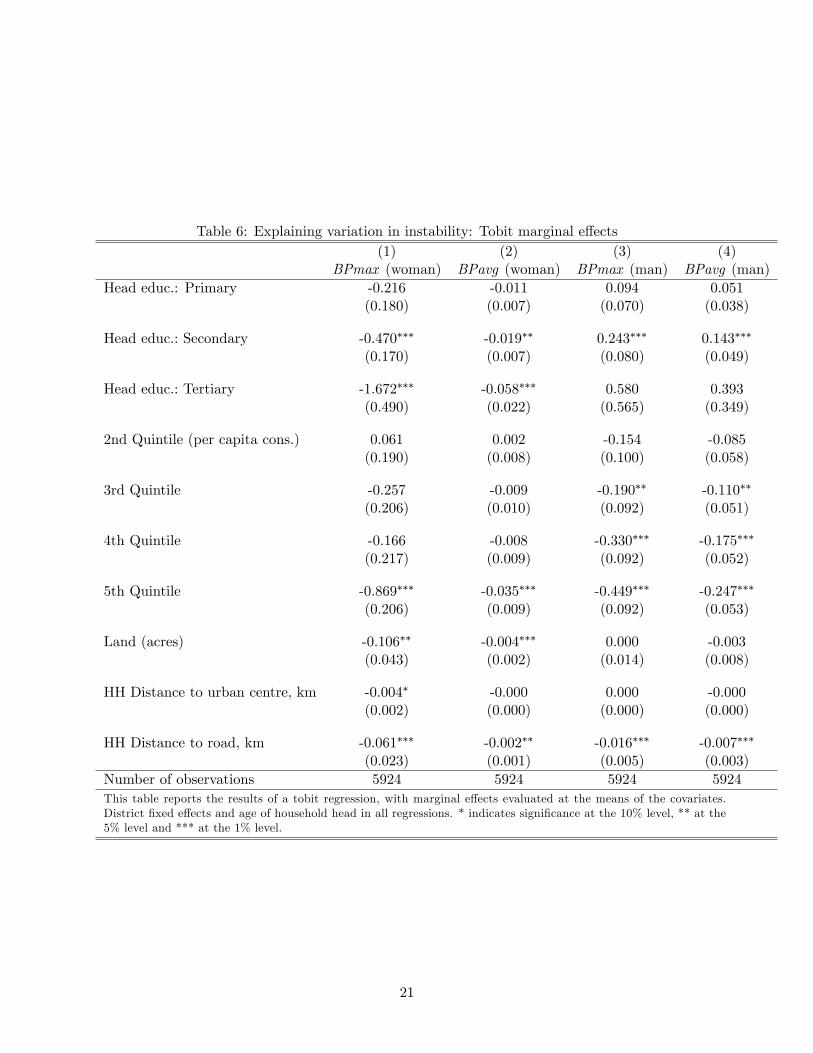
Table 6: Explaining variation in instability: Tobit marginal e¤ects(1) (2) (3) (4)

BPmax (woman) BPavg (woman) BPmax (man) BPavg (man)Head educ.: Primary -0.216 -0.011 0.094 0.051

(0.180) (0.007) (0.070) (0.038)

Head educ.: Secondary -0.470��� -0.019�� 0.243��� 0.143���

(0.170) (0.007) (0.080) (0.049)

Head educ.: Tertiary -1.672��� -0.058��� 0.580 0.393(0.490) (0.022) (0.565) (0.349)

2nd Quintile (per capita cons.) 0.061 0.002 -0.154 -0.085(0.190) (0.008) (0.100) (0.058)

3rd Quintile -0.257 -0.009 -0.190�� -0.110��

(0.206) (0.010) (0.092) (0.051)

4th Quintile -0.166 -0.008 -0.330��� -0.175���

(0.217) (0.009) (0.092) (0.052)

5th Quintile -0.869��� -0.035��� -0.449��� -0.247���

(0.206) (0.009) (0.092) (0.053)

Land (acres) -0.106�� -0.004��� 0.000 -0.003(0.043) (0.002) (0.014) (0.008)

HH Distance to urban centre, km -0.004� -0.000 0.000 -0.000(0.002) (0.000) (0.000) (0.000)

HH Distance to road, km -0.061��� -0.002�� -0.016��� -0.007���

(0.023) (0.001) (0.005) (0.003)Number of observations 5924 5924 5924 5924This table reports the results of a tobit regression, with marginal e¤ects evaluated at the means of the covariates.District �xed e¤ects and age of household head in all regressions. * indicates signi�cance at the 10% level, ** at the5% level and *** at the 1% level.

21

5.2 Divorce

We now present the main empirical analysis. We examine whether our instability indices, estimated

using 2010 data, can predict divorce in the following three years. We estimate a logit model of

divorce between 2010 and 2013, with the BP indices of the spouses and the IR index of the husband

as covariates. We do not include the wife�s IR index because this measure does not not vary in

our sample. In addition to the covariates in the regressions in Table 6, we also include variables

to measure religiousness in the village (the number of churches and the number of mosques), an

additional measure of connectivity (access to a telephone in the village) and measures of match

quality (the education, age and religion di¤erence of the spouses). Finally, we also include the size

of the cluster as a control variable. The results are in Table 7.

Interestingly, we �nd a signi�cant relationship between the instability indices from our structural

model and subsequent divorce. In regression (1), a one-percentage-point increase in the wife�s

maximum gain from remarriage, as a proportion of her household�s income, raises the probability

of divorce by 0:6 percentage points on average. This is a non-negligible e¤ect, as the proportions of

currently divorced and married individuals in the population suggest an annual divorce probability

of approximately 8:5%. In regression (2), a one-percentage-point increase in the average remarriage

gain for the wife, as a proportion of her household�s income, raises divorce probability by 17:9

percentage points. Note that the impact of a percentage point change of the maximum and average

gains from remarriage on the divorce probability are not directly comparable to each other since

the base levels of the BPmax and BPavg are very di¤erent (see Table 3). The BPavg index of the

husband also has a positive, signi�cant e¤ect on divorce probability, although the e¤ect is small in

magnitude compared to that of the wife�s BPavg index. Next, we �nd that the IR index of the man

has a slightly negative, but statistically signi�cant, impact on divorce. This may seem surprising

at �rst sight. However, as we will explain further on (when discussing Table 9), this negative e¤ect

of the male�s IR index disappears if we condition on wages, non-labour incomes and land incomes

and, therefore, it may be regarded as mainly capturing an income e¤ect. Overall, these results

suggest that our measures of instability are able to capture the gains to divorce, and that women

in Malawi are more likely to divorce for economic reasons than men. These results validate our

structural model.

Other covariates are also signi�cantly related to divorce. The probability of divorce is decreasing

in the number of children, with an additional child reducing divorce probability by 1:4 percentage

points. This implies that an approximately 2:3 percentage point reduction in the wife�s maximum

gain from remarriage, as a percentage of income, reduces divorce probability as much as an addi-

tional child. The probability of divorce is falling in the age of the household head, which may be

because couples who are together longer are better matched, or because the value of outside options

on the marriage market falls with age. We also �nd that divorce probability is decreasing in the

household�s wealth, as captured by the per capita consumption quintile. This is consistent with

the descriptive statistics in Section 4. In villages with many mosques, divorce is less likely, while

divorce is more likely in villages with a telephone, again suggesting that connectedness plays an

22

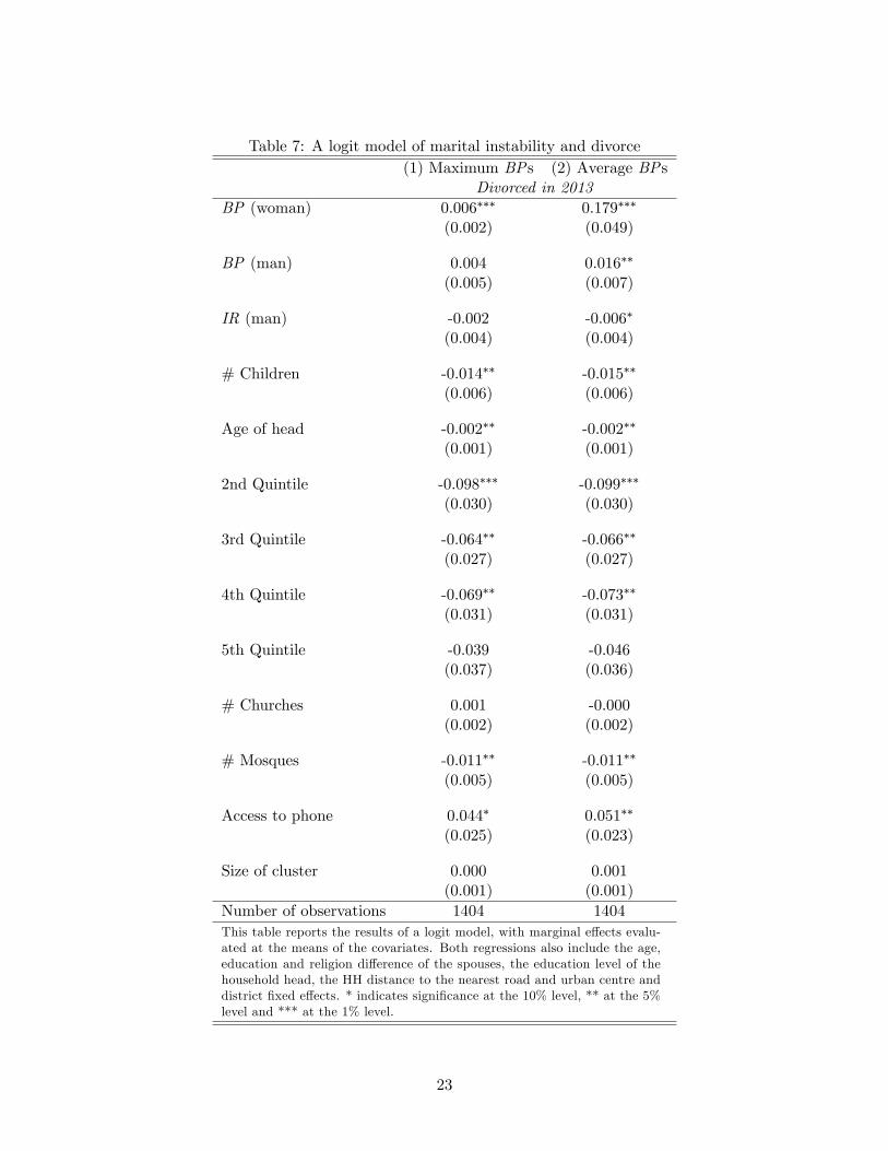
Table 7: A logit model of marital instability and divorce(1) Maximum BPs (2) Average BPs

Divorced in 2013BP (woman) 0.006��� 0.179���

(0.002) (0.049)

BP (man) 0.004 0.016��

(0.005) (0.007)

IR (man) -0.002 -0.006�

(0.004) (0.004)

# Children -0.014�� -0.015��

(0.006) (0.006)

Age of head -0.002�� -0.002��

(0.001) (0.001)

2nd Quintile -0.098��� -0.099���

(0.030) (0.030)

3rd Quintile -0.064�� -0.066��

(0.027) (0.027)

4th Quintile -0.069�� -0.073��

(0.031) (0.031)

5th Quintile -0.039 -0.046(0.037) (0.036)

# Churches 0.001 -0.000(0.002) (0.002)

# Mosques -0.011�� -0.011��

(0.005) (0.005)

Access to phone 0.044� 0.051��

(0.025) (0.023)

Size of cluster 0.000 0.001(0.001) (0.001)

Number of observations 1404 1404This table reports the results of a logit model, with marginal e¤ects evalu-ated at the means of the covariates. Both regressions also include the age,education and religion di¤erence of the spouses, the education level of thehousehold head, the HH distance to the nearest road and urban centre anddistrict �xed e¤ects. * indicates signi�cance at the 10% level, ** at the 5%level and *** at the 1% level.

23

important role in household dissolution. Finally, the size of the cluster is not signi�cantly related

to divorce.

It is worth noting that the absence of domestic labour cannot explain the signi�cant e¤ect of the

wife�s instability index on divorce. As domestic labour is currently included in leisure, marriages

appear to be more attractive than they actually are. Consider a woman who engages in a lot of

domestic labour: she appears to be stable, but at the same time is unhappy because she works hard,

as a result of which she is more likely to divorce. An increase in domestic labour increases stability

in our model but at the same time is likely to increase the probability of divorce. Therefore, it

cannot explain the positive relationship between the instability indices and divorce probability.

Finally, our results cannot be explained by polygamy. The inclusion of a dummy for the existence

of polygamy in the village does not a¤ect the signi�cant e¤ect of the wife�s instability index on

divorce, but we do �nd that the existence of polygamy increases the overall probability of divorce

(results available on request).

5.3 Extensions

Multinomial model An important implication of the way that the instability indices are de�ned

is that the BP index measures the attractiveness of a potential new match on the marriage market,

while the IR index measures the attractiveness of being single. Therefore, we should observe these

associations in the data as well. In order to explore this, we estimate a multinomial logit model

for the marital status of husbands and wives in 2013, distinguishing between remarriage and being

single.9 We retain the same right-hand side variables as in Table 7 and set remaining married

as the base case. The results are in Table 8, which reports relative risk ratios (exponentiated

coe¢ cients).10

The results are consistent with the premise that the BP indices measure the attractiveness of

remarriage. In particular, a higher value of the husband�s BP index is signi�cantly associated with

a higher probability that the husband divorces and remarries in the next three years, instead of

remaining married. The e¤ect of the wife�s BP index is stronger and is signi�cantly associated with

the remarriage of both the husband and the wife. This result is consistent with the observation that

in Malawi, men �nd it easy to remarry. A one percentage point increase in the wife�s maximum

remarriage gain, as a proportion of household income, raises the relative risk of both the husband

and wife divorcing and remarrying, relative to remaining married, by a factor of 1:1. Neither the

wife�s nor the husband�s BP index raises the odds of divorcing and being single, relative to staying

married; this is encouraging, as blocking pairs relate speci�cally to potential remarriage partners

and should not be related to individuals divorcing in order to be single. Therefore, the BP indices

9The multinomial logit model assumes Independence of Irrelevant Alternatives (IIA). A more general model is thenested logit, which allows for correlation between alternatives. We estimated a nested logit model for marital statuswith a reduced set of district dummy variables, as the model did not converge with the full set. In this restrictedversion of the nested logit model, the IIA assumption was not rejected. Therefore, we proceeded with the multinomiallogit model.10The sample size in these estimates is lower than in the previous table because we do not know the marital status

of every divorced man and woman (see also the explanation in Section 3.2).

24

Table 8: Multinomial logit regressions on marital status(1) - Marital status of man (2) - Marital status of womanRemarried Single Remarried Single

BPmax (woman) 1.134��� 0.968 1.088�� 1.033

(0.036) (0.062) (0.039) (0.039)

BPmax (man) 1.160� 1.004 0.927 1.025

(0.091) (0.168) (0.116) (0.065)

IR (man) 0.944 1.023 0.945 1.068

(0.064) (0.115) (0.058) (0.057)

# Children 0.961 0.628��� 0.804�� 0.855

(0.090) (0.063) (0.072) (0.096)

Age of head 0.970� 0.995 0.967�� 0.978(0.016) (0.022) (0.015) (0.014)

2nd Quintile 0.451 0.074�� 0.325�� 0.323��

(0.221) (0.094) (0.144) (0.178)

3rd Quintile 0.586 0.182�� 0.324��� 0.650

(0.273) (0.145) (0.142) (0.290)

4th Quintile 0.466 0.295� 0.503� 0.198���

(0.257) (0.217) (0.209) (0.105)

5th Quintile 1.498 0.011��� 0.313� 0.494

(0.770) (0.018) (0.190) (0.312)

# Churches 1.001 0.964 0.990 1.033

(0.022) (0.046) (0.031) (0.036)

# Mosques 0.830��� 0.857 0.949 0.883�

(0.059) (0.094) (0.062) 0.061

Access to phone 1.908� 0.470 2.050�� 1.505

(0.716) (0.368) (0.616) (0.591)

Size of cluster 1.005 0.989 1.003 1.024�

(0.009) (0.026) (0.010) 0.014

Number of observations 1345 1378This table reports relative risk ratios (standard error) from a multinomial logit model. All regressionsalso include the age, education and religion di¤erence of the spouses, the education level of thehousehold head, the HH distance to the nearest road and urban centre and district �xed e¤ects.District FEs for regression (2) are an aggregated version of those for regression (1), due to insu¢ cientvariation in the outcome in some districts. * indicates signi�cance at the 10% level, ** at the 5%level and *** at the 1% level.

25

appear to capture the attractiveness of remarriage in particular. The husband�s IR index does not

a¤ect the odds of either divorce status, relative to remaining married. This may be because the

values of the IR indices are very low in general, with little variation; because few men are observed

to be single in the data; or because there are unobserved bene�ts to being married.

Other signi�cant e¤ects persist from Table 7: the odds of a woman divorcing and remarrying are

declining in the number of children, as are the odds that a man divorces and remains single. The

number of mosques has a signi�cant negative e¤ect on the odds that the man divorces and remarries,

as well as the odds that the woman divorces and remains single. The presence of a telephone in the

village increases the odds of remarriage for both the husband and wife but, interestingly, has no

e¤ect on the odds that either spouse is single. This supports the idea that the telephone captures

some of the ability of spouses to learn about their marriage market. Finally, a higher consumption

quintile of the household is broadly associated with lower odds of divorce for the wife, consistent

with the results in Table 7, which showed that wealthier households are less likely to divorce.

Can the e¤ect of instability be explained by wages or income? The results so far suggest

that individuals, and particularly women, in Malawi divorce for economic reasons and that our

instability indices capture these economic reasons well. However, one might argue that the BP

index does not capture the economic gains from divorce, but rather is entirely driven by one or

more of its components from equation (8) in Section 2.3. In order to explore this possibility, we

introduce these components as explanatory variables to regressions (1) and (2) in Table 7. In

particular, we include the average wage of the husband and wife, the di¤erence between these

wages, the average non-labour income of the spouses, its di¤erence, as well as the average land

income, its di¤erence, and the log of total income. All of these variables are the product of the

estimation discussed in Section 2.4. The results are in Table 9.

The key result is that the coe¢ cients on the BP indices in this table are not signi�cantly

di¤erent from those in the regressions in Table 7. In other words, the e¤ect of our instability

index cannot be explained simply by di¤erences in wages, non-labour income or land income of

the spouses. These variables do seem to explain the negative impact of the IR index of the man,

however, indicating that this index is mainly capturing an income e¤ect. As such we can conclude

that the BP indices are able to capture a more complex form of gains from divorce that likely

includes intrahousehold sharing of consumption, which is an important determinant of the BP

indices in the model. Finally, we �nd that the average wage and the non-labour income of the

household have a signi�cant decreasing e¤ect on the probability of divorce, beyond any indirect

e¤ect through the BP indices. Presumably, this is because they increase the gains to the current

marriage. The same conclusion does not hold for land income and total income, but note that the

impact of these variables is rather small compared to all the other variables.

Heterogeneous e¤ects We have shown that spouses�BP indices are signi�cantly associated

with divorce, that this result holds in a multinomial model and that it cannot be explained by the

components of the BP indices from the structural model. This relationship may mask signi�cant

26

Table 9: Explaining the e¤ect of instability with its individual components(1) Maximum BPs (2) Average BPs

Divorced in 2013BP (woman) 0.006��� 0.161���

(0.002) (0.048)

BP (man) 0.002 0.013�

(0.005) (0.007)

IR (man) 0.001 -0.004(0.004) (0.004)

Wage (avg.) -0.005�� -0.006��

(0.002) (0.002)

Wage (di¤.) -0.001 -0.001(0.001) (0.001)

NLI (avg., 000s) -0.001�� -0.001��

(0.000) (0.000)

NLI (di¤., 000s) 0.000 0.000(0.000) (0.000)

Land income (avg., 000s) -0.002 -0.002(0.001) (0.001)

Land income (di¤., 000s) 0.001� 0.001�

(0.001) (0.001)

Log(total income) 0.539�� 0.574��

(0.225) (0.223)Number of observations 1404 1404This table reports the results of a logit regression, with marginal e¤ects eval-

uated at the means of the covariates. Both models also include the same

right-hand side variables as in Table 7. * indicates signi�cance at the 10%

level, ** at the 5% level and *** at the 1% level.

27

heterogeneity, and this is what we explore here. We focus on the most attractive remarriage

possibility (BPmax ) and we include some new variables in the logit model of Table 7, such as

landholdings and the sex ratio (de�ned as the ratio of males over females in a given cluster), as

well as explore heterogeneity in existing explanatory variables, namely age of the household head

and number of children. Table 10 shows these results.

In regression (1), we �nd that the signi�cant e¤ect of BPmax on divorce only holds when the

household has positive landholdings, and is increasing in these landholdings. For a household that

owns two acres of land, which are the average landholdings in our sample, an increase in the wife�s

BPmax of one percentage point increases the probability of divorce by 0:6 percentage points, which

is comparable to the e¤ect in Table 7. The result also makes intuitive sense: land provides security

on divorce, so spouses without land may �nd it too economically risky to divorce.

Next, we consider the interaction between age and the BPmax indices. Regression (2) shows

that the wife�s BPmax index is still a signi�cant predictor of divorce, but this e¤ect is declining in

the age of the household head. This may be for two reasons: �rst, age may be a proxy for marital

duration, and assuming match quality is revealed over time, spouses may be less driven by economic

incentives later on in marriage. Second, age may tell us something about the individual�s outside

options. An older divorcée may have lower chances on the remarriage market than a younger

divorcée, all other things equal, so that she may be less likely to respond to attractive outside

options.

In the baseline regressions in Table 7, children always reduce the probability of divorce. In

regression (3), we �nd that this is especially true for men: high remarriage gains for the husband are

less likely to result in divorce if the couple has more children. This is also true for the wife, although

the e¤ect is not statistically signi�cant. Finally, in regression (4) we examine the interaction

between the sex ratio and the e¤ect of blocking pairs on divorce. For a sex ratio equal to one,

an increase in the wife�s BPmax index of one percentage point increases the probability of divorce

by approximately 1:6 percentage points. The more men there are, relative to women, the stronger

the e¤ect of the wife�s potential gains from remarriage on divorce probability. This is a rational

response: if there are more men relative to women in the population, the likelihood of a pro�table

remarriage is greater.

6 Conclusion

We have de�ned structural measures of the gains from divorce and shown that they are signi�cant

predictors of future divorces. These measures are based on a collective model with consumption

and agricultural production embedded in a marriage market. The key theoretical contribution

is that we extend Cherchye, Demuynck, De Rock and Vermeulen (2015) to include agricultural

production, allowing the estimation of shadow wages and land prices. The model yields marital

stability conditions for each married individual. Using these conditions, we can quantify marital

instability in terms of Individual Rationality (IR) and Blocking Pair (BP) indices, which capture

28

Table 10: Heterogeneous e¤ects of blocking pairs(1) (2)

Divorced in 2013 Divorced in 2013BPmax (woman) 0.001 BPmax (woman) 0.018��

(0.003) (0.007)

Land*BPmax (woman) 0.003��� Age*BPmax (woman) -0.0003�

(0.001) (0.000)

BPmax (man) 0.007 BPmax (man) 0.024(0.008) (0.019)

Land*BPmax (man) -0.003 Age*BPmax (man) -0.001(0.003) (0.001)

Land Age -0.001(0.011) (0.001)

Number of observations 1404 Number of observations 1404

(3) (4)Divorced in 2013 Divorced in 2013

BPmax (woman) 0.011��� BPmax (female) -0.040���

(0.004) (0.015)

Children*BPmax (woman) -0.002 Sex ratio*BPmax (female) 0.056���

(0.001) (0.018)

BPmax (man) 0.018� BPmax (man) 0.019(0.009) (0.020)

Children*NBPmax (man) -0.007�� Sex ratio*BPmax (man) -0.015(0.003) (0.022)

Children -0.008 Sex ratio -0.225(0.008) (0.154)

Number of observations 1404 Number of observations 1404This table reports the results of a logit model, with marginal e¤ects evaluated at the means of the covariates. All

regressions in this table include the same right-hand side variables as in Table 7. * indicates signi�cance at the

10% level, ** at the 5% level and *** at the 1% level.

29

spouses� consumption gains to remarrying another individual in the same marriage market (BP

index) and to being single (IR index).

We estimate our model on the 2010 wave of the Malawi Integrated Household Survey, and

correlate our instability indices with divorce in the next three years of the panel data set. We �nd

that a 1 percentage point increase in the wife�s BP index as a proportion of her household income

increases divorce probability by 0:6 percentage points in the next three years. This result is robust

to using an average BP or most attractive BP index, as well as to the estimation of a more general

multinomial model. We also show that this result cannot be explained by the wages or land income

of the spouses, implying that intrahousehold sharing matters.

Our �ndings lead us to conclude that divorce in Malawi is driven, at least partly, by economic

considerations of spouses, with consumption sharing within households as an important deter-

minant. In addition, our empirical results validate the set-up of our theoretical model. More

generally, they show the value-added of adopting a Beckerian approach that analyzes marriage de-

cisions through the lens of a structural model of household decision making. Finally, as agricultural

productivity is a key determinant of outside options in developing countries reliant on agriculture,

our model is applicable to other contexts as well, where accurate data on wages or land prices may

not be available.

References

[1] Afriat, S.. �The Construction of Utility Functions from Expenditure Data." International

Economic Review 8 (1967): pp. 67-77.

[2] Afriat, S.. �E¢ ciency Estimation of Production Functions." International Economic Review

13 (1972): pp. 568-598.

[3] Becker, G. S.. �A Theory of Marriage: Part I." Journal of Political Economy 81 (1973): pp.

813-846.

[4] Becker, G. S.. �A Theory of Marriage: Part II." Journal of Political Economy 82 (1974): pp.

S11-S26.

[5] Becker, G. S., E. M. Landes and R. T. Michael. �An Economic Analysis of Marital Instability."

Journal of Political Economy 85 (1977): pp. 1141-1187.

[6] Bignami-Van Assche, S., A. Van Assche, P. Anglewicz, P. Fleming and C. van de Ruit.

�HIV/AIDS and Time Allocation in Rural Malawi." Demographic Research 24 (2011): pp.

671-708.

[7] Blundell, R., P.-A. Chiappori, T. Magnac, and C. Meghir. �Collective labour supply: hetero-

geneity and nonparticipation." Review of Economic Studies 74 (2007): pp. 417-445.

30

[8] Boheim, R. and J. Ermisch. �Partnership Dissolution in the UK - the Role of Economic

Circumstances." Oxford Bulletin of Economics and Statistics 63 (2001): pp. 197-208.

[9] Brien, M., L. Lillard, and S. Stern. �Cohabitation, Marriage, and Divorce in a Model of Match

Quality." International Economic Review 47 (2006): pp. 451-494.

[10] Browning, M., P.-A. Chiappori, and Y. Weiss. Economics of the Family (2014), Cambridge

University Press.

[11] Charles, K. K. and M. Stephens, Jr.. �Job Displacement, Disability and Divorce." Journal of

Labour Economics 22 (2004): pp. 489-522.

[12] Cherchye, L., T. Demuynck, B. De Rock and F. Vermeulen. �Household Consumption when

the Marriage is Stable." (2015). Mimeo.

[13] Cherchye, L., B. De Rock, A. Lewbel, and F. Vermeulen. �Sharing Rule Identi�cation for

General Collective Consumption Models." Econometrica 83 (2015): pp. 2001-2041.

[14] Cherchye, L., B. De Rock, and F. Vermeulen. �The collective model of household consumption:

a nonparametric characterization." Econometrica 75 (2007): pp. 553-574.

[15] Cherchye, L., B. De Rock, and F. Vermeulen. �Opening the black box of intra-household

decision-making: theory and non-parametric empirical tests of general collective consumption

models." Journal of Political Economy 117 (2009): pp. 1074-1104.

[16] Cherchye, L., B. De Rock, and F. Vermeulen. �The revealed preference approach to collective

consumption behavior: testing and sharing rule recovery." Review of Economic Studies 78

(2011): pp. 176-198.

[17] Cherchye, L., B. De Rock and F. Vermeulen. �Married with Children: a Collective Labor

Supply Model with Detailed Time Use and Intrahousehold Expenditure." American Economic

Review 102 (2012): pp. 3377-3405.

[18] Chiappori, P.-A.. �Rational Household Labour Supply." Econometrica 56 (1988): pp. 63-89.

[19] Chiappori, P.A.. �Collective Labour Supply and Welfare." Journal of Political Economy 100

(1992): pp. 437-467.

[20] Chiappori, P.A.. �Introducing household production in the collective model of labour supply."

Journal of Political Economy 105 (1997): pp. 191-209.

[21] Davison, J.. �Tenacious Women: Clinging to Banja Household Production in the Face of

Changing Gender Relations in Malawi." Journal of Southern African Studies 19 (1993): pp.

405-421.

[22] Davison, J.. Gender, Lineage and Ethnicity in Southern Africa. Oxford: Westview Press, 1997.

31

[23] Diewert, E.. �Afriat and Revealed Preference Theory�, Review of Economic Studies 40 (1973):

pp. 419-426.

[24] Dunbar, G. R., A. Lewbel and K. Pendakur. �Children�s Resources in Collective Households:

Identi�cation, Estimation, and an Application to Child Poverty in Malawi." American Eco-

nomic Review 103 (2013): pp. 438-471.

[25] Ellis, F., M. Kutengule and A. Nyasulu. �Livelihoods and Rural Poverty Reduction in Malawi."

World Development 31 (2003): pp. 1495-1510.

[26] Farnham, M., L. Schmidt and P. Sevak. �House Prices and Marital Stability." American Eco-

nomic Review Papers & Proceedings 101 (2011): pp. 615-619.

[27] Gale, L.S., and D. Shapley. �College admissions and the stability of marriage�. American

Mathematical Monthly 69 (1962): pp. 9-15.

[28] Hankins, S. and M. Hoekstra. �Lucky in Life, Unlucky in Love? The E¤ect of Random Income

Shocks on Marriage and Divorce." Journal of Human Resources 46 (2011): pp. 403-426.

[29] Kerr, R. B.. �Informal Labor and Social Relations in Northern Malawi: The Theoretical

Challenges and Implications of Ganyu Labour for Food Security." Rural Sociology 70 (2005):

pp. 167-187.

[30] Jovanovic, B.. �Job Matching and the Theory of Turnover". Journal of Political Economy 87

(1979): pp. 972-990.

[31] Mwambene, L.. �Divorce in Matrilineal Customary Law Marriage in Malawi: A Compara-

tive Analysis with the Patrilineal Customary Law Marriage in South Africa." LLM Thesis

University of Western Cape (2005).

[32] Pollak, R.A. and M.L. Wachter. �The relevance of the household production function and its

implications for the allocation of time." Journal of Political Economy 83 (1975): pp. 255-277.

[33] Reniers, G.. �Divorce and Remarriage in Rural Malawi." Demographic Research Special Col-

lection 1.6 (2003).

[34] Samuelson, P.. �A note on the pure theory of consumers behaviour�. Economica 5 (1938): pp.

61-71.

[35] Takane, T.. �Customary Land Tenure, Inheritance Rules and Smallholder Farmers in Malawi."

Journal of Southern African Studies 34 (2008): pp. 269-291.

[36] Telalagic, S. "Moral Hazard in Marriage: The Use of Domestic Labour as an Incentive Device."

(2015). Mimeo.

[37] Telalagic, S. �Kinship and Consumption: The E¤ect of Spouses�Outside Options on Household

Productivity." (2015). Mimeo.

32

[38] Varian, H.. �The Nonparametric Approach to Demand Analysis." Econometrica 50 (1982):

pp. 945-972.

[39] Varian, H.. �The Non-Parametric Approach to Production Analysis." Econometrica 52 (1984):

pp. 579-598.

[40] Weiss, Y. and R. Willis. �Match Quality, New Information and Marital Dissolution." Journal

of Labour Economics 15.1.2 Essays in Honour of Yoram Ben-Porath (1997): pp. S293-S329.

[41] World Bank Development Economics Research Group and Malawi National Statistical O¢ ce.

Malawi Living Standards Measurement Study: 2010-2013 IHS3 Survey (2015).

Appendix: data construction

All values used in our empirical application were converted to real terms using the spatial and

temporal price index provided in the IHS. In some cases we recoded outliers, namely the top 1%

of values, to be equal to the value at the 99th percentile. This was because in those cases the top

1% of values were not sensible, given the context of the data.

Bounds on wages and land prices

Wages We calculated the median observed wage per hour of hired workers in the district,

separately for males and females. Where there were insu¢ cient observations, we used the regional

median instead. The bounds were zero and two times this median.

Land price per acre For each plot of owned land, households were asked how much they

could earn if they rented it out for one year. We regressed this value on plot characteristics: the

size of the plot; the soil type of the plot; the soil quality of the plot; whether the plot is swamp

or wetland; and how the household acquired the plot. We then used the predicted values of this

regression to estimate the rental income for those plots where the reported rental income was

missing. The rental income was summed for each household and divided by the total acres of land,

giving an average rental income per acre for each household. We then obtained the median rental

income per acre for each village and for each district. We used the median rental income per acre

for the village where there were at least seven observations per village; where there were fewer, we

used the median rental income per acre for the district. The bounds on the land price were zero

and two times this median.

Production

Inputs We calculated the cost of inputs into production as the total of direct inputs, such

as the costs of fertilizer, seeds and transport, the cost of indirect inputs, namely machinery, and the

cost of hired labour. For machinery, we calculated the use value of each item by �rst calculating the

33

remaining age of the item as twice the mean age of this item in the sample minus its current age,

with a minimum of two years. The annual consumption stream from each item was the amount of

money the item could be sold for, if sold today, divided by the remaining age of the item. The cost

of hired labour was calculated as the number of days this labour was used times the average daily

wage for these labourers, as reported by the household. The survey distinguished between male,

female and child labourers, providing a more accurate measure of the total cost. Free labour was

also valued at these rates and included as a costly input.

Revenue The revenue was calculated as the sum of all crop sales during the rainy and dry

seasons and the value of all own agricultural production that was consumed by the household.

The latter value originates from the survey itself, where households were asked how much of each

consumed food they had grown themselves. This was then valued at local prices by the World Bank

Living Standards Measurement Study team.11

Consumption

Consumption was split into four categories: public consumption; private non-assignable consump-

tion; private consumption of the man and private consumption of the woman.

Public consumption This included expenditure on children�s education and health, expendi-

ture on the education and health of other household members (not the husband or wife), expenditure

on children�s clothing, expenditure on durables (which was calculated as a use value or consumption

stream, using the same method described for machinery above), expenditure on public nondurables

(such as candles, light bulbs and books), expenditure on rent and expenditure on public bills (such

as �rewood and the landline telephone).

Private non-assignable consumption The largest component of private non-assignable con-

sumption was food, consisting of food purchased, the value of food from own production and the

value of food received as a gift. This category also included private bills (such as the mobile tele-

phone) and private nondurables (such as cigarettes, tickets for public transport, soap and stationery

items).

Private consumption of the man and woman This consisted of the health, education and

clothing expenses of the man or woman.

Time

The model requires two time variables: agricultural labour and leisure.

11Many thanks to Talip Kilic for sharing his Stata code that allowed us to separately identify consumption fromown production and consumption from purchases.

34

Agricultural labour Agricultural labour was calculated as the total number of hours of agri-

cultural work on the household�s plots in the rainy and dry seasons of the past year, reported by

the husband or wife. Where certain information was missing, such as the individual reported the

number of days worked but not the number of hours per day, we used the village median for this

information, where there were at least seven observations in the village. Otherwise, we used the

district median.

Leisure In order to calculate leisure hours, we �rst required a measure of total available hours.

As reported working hours are fairly low, leading to likely overestimates of true leisure time, we

calculated total time available as the number of hours worked by the hardest working man or woman

in the sample in the past year. This included both agricultural and wage labour and resulted in

a value of 6120 hours. We assumed that this hardest worker works full-time and has zero leisure.

We then calculated leisure for each individual as 6120 minus the annual hours of agricultural and

wage labour of each individual.

Landholdings

In order to accurately measure the land income of individuals on divorce, we required exact in-

formation on the amount of land owned by each spouse. We de�ned land to be owned if it was

inherited, granted by local leaders, part of a bride price, purchased with a title or purchased with-

out a title. Land that was owned either solely by the spouse or owned by the spouse jointly with

someone outside the household was assumed to accrue to that spouse on divorce. Land not owned

by either spouse was assumed to disappear after divorce, while land owned jointly by the spouses

was allowed to be endogenously split in the simulations.

Covariates in regressions

Here we explain how the covariates in the regressions were de�ned. All covariates from the data

are from the 2010 wave. The 2013 wave was only used to see whether the couple had divorced.

# Children This is the number of own or adopted children living in the household.

Consumption quintiles This splits the entire sample into �ve sections, in terms of per capita

consumption. The �rst quintile is a dummy variable that equals one if the household is in the

bottom 20% of per capita consumption in the full IHS sample and zero otherwise, while the �fth

quintile is a similar de�nition for households in the top 20%. Other quintiles are de�ned analogously.

Age of head This is the age of the household head; the identity of the head was self-reported in

the data.

35

Head education level This is a series of dummy variables that de�ne the highest education

level of the head, which ranges from no education to tertiary education.

Diploma di¤erence This is the husband�s highest achieved diploma minus the wife�s highest

achieved diploma. The highest achieved diploma ranges from 1 (none) to a 7 (post-graduate

degree). The di¤erence ranges from -3 to 6 in our sample.

Age di¤erence This is the husband�s age minus the wife�s age.

Religion di¤erence This is a dummy variable that equals one if the spouses are of a di¤erent

religious denomination, and zero otherwise.

# Churches/ #Mosques This is the number of churches/mosques in the village, as reported

by village informants.

Distance to road, urban centre This is the household�s distance to the nearest road or nearest

urban centre (Lilongwe, Zomba or Blantyre) in kilometers.

Access to phone This is a dummy variable that equals one if there is a place in the village to

make a phonecall, and zero otherwise.

Sex ratio This is the ratio of men to women at the cluster level in the IHS sample, calculated

based on the heads of household. Single-headed households count as one male or one female, while

married households count as one male and one female.

Land This is the total number of acres of land owned by the household.

Size of cluster This is the total number of households in that particular household�s marriage

market cluster, de�ned using the method described in Section 3.2.

Public/private share of consumption This is the share of public or private consumption in

total consumption.

Nonlabour income (NLI) This is an output of the structural model and is the di¤erence

between total consumption and other inputs on the one hand and labour and land income on the

other hand .

Land income This is an output of the structural model and gives the total number of acres of

land owned by the spouse multiplied by the shadow price of land. It measures the annual rental

yield on the land.

36

Wage This is an output of the structural model and gives the hourly shadow wage of agricultural

labour of the husband or wife.

37