When Work Disappears: Manufacturing Decline and the Falling

Marriage-Market Value of Men

∗

David Autor† David Dorn‡ Gordon Hanson§

March 2017

Abstract

The structure of marriage and child-rearing in U.S. households has undergone two markedshifts in the last three decades: a steep decline in the prevalence of marriage among young adults,and a sharp rise in the fraction of children born to unmarried mothers or living in single-headedhouseholds. A potential contributor to both phenomena is the declining labor-market oppor-tunities faced by males, which make them less valuable as marital partners. We exploit largescale, plausibly exogenous labor-demand shocks stemming from rising international manufactur-ing competition to test how shifts in the supply of young ‘marriageable’ males affect marriage,fertility and children’s living circumstances. Trade shocks to manufacturing industries haveparticularly negative impacts on the labor market prospects of men and degrade their marriage-market value along multiple dimensions: diminishing their relative earnings—particularly at thelower segment of the distribution—reducing their physical availability in trade-impacted labormarkets, and increasing their participation in risky and damaging behaviors. As predicted by asimple model of marital decision-making under uncertainty, we document that adverse shocks tothe supply of ‘marriageable’ men reduce the prevalence of marriage and lower fertility but raisethe fraction of children born to young and unwed mothers and living in in poor single-parenthouseholds. The falling marriage-market value of young men appears to be a quantitativelyimportant contributor to the rising rate of out-of-wedlock childbearing and single-headed chil-drearing in the United States.

Keywords: Marriage Market, Fertility, Household Structure, Single-Parent Families, TradeFlows, Import Competition, Local Labor Markets

JEL Classifications: F16, J12, J13, J21, J23

∗This paper previously circulated under the title “The Labor Market and the Marriage Market” (first circulatingdraft May 12, 2014). Autor, Dorn and Hanson acknowledge funding from the Russell Sage Foundation (RSF Project#85-12-07). Dorn acknowledges funding from the Spanish Ministry of Science and Innovation (grants CSD2006-00016and ECO2010-16726) and the Swiss National Science Foundation (grant BSSGI0-155804). Autor and Hanson ac-knowledge funding from the National Science Foundation (grant SES-1227334). We thank Andrew Cherlin, MariannePage, Ann Huff Stevens, Kathleen Vohs, Jane Waldfogel, and numerous seminar and conference participants for valu-able suggestions. We are grateful to Ante Malenica, Timothy Simmons, Juliette Thibaud, and Melanie Wassermanfor expert research assistance.

†MIT Department of Economics and NBER. E-mail: dautor@mit.edu‡University of Zurich and CEPR. E-mail: david.dorn@econ.uzh.ch§UC San Diego and NBER. E-mail: gohanson@ucsd.edu

“The consequences of high neighborhood joblessness are more devastating than those

of high neighborhood poverty. A neighborhood in which people are poor but employed

is different from a neighborhood in which people are poor and jobless. Many of today’s

problems in the inner-city ghettos—crime, family dissolution, welfare, low levels of social

organization, and so on—are fundamentally a consequence of the disappearance of work.”

William Julius Wilson, When Work Disappears, 1996, pp. xiii.

“Wilson’s book spoke to me. I wanted to write him a letter and tell him that he had

described my home perfectly. That it resonated so personally is odd, however, because

he wasn’t writing about the hillbilly transplants from Appalachia—he was writing about

black people in the inner cities.” J.D. Vance, Hillbilly Elegy: A Memoir of Family and

Culture in Crisis, 2016, p. 144.

1 Introduction

Marriage and child-rearing in U.S. households has undergone two marked shifts in the last three

decades. A first is the steep decline in marriage rates among young adults, particularly for the less-

educated. Between 1979 and 2008, the share of U.S. women between the ages of 25 and 39 who were

currently married fell by 10 percentage points among the college-educated, by 15 percentage points

among those with some college but no degree, and by fully 20 percentage points among women with

high-school education or less (Autor and Wasserman, 2013). These declines reflect rising age at first

marriage, a decline in lifetime marriage rates and, to a lesser extent, a rise in divorce among less-

educated women (Bailey and DiPrete, 2016; Cherlin, 2010; Greenwood, Guner and Vandenbroucke,

forthcoming; Heuveline, Timberlake and Furstenberg, 2003). Accompanying the decline in marriage

is an increase in the share of children born out of wedlock and living in single-headed households.

The fraction of U.S. children born to unmarried mothers more than doubled between 1980 and 2013,

rising from 18 to 41 percent (Martin, Hamilton, Osterman, Curtin and Matthews, 2015).

The causes of the decoupling of marriage from child-rearing has drawn decades of research and

policy attention. Among the most prominent entries in this debate are William Julius Wilson’s

pioneering book, The Truly Disadvantaged (Wilson, 1987), followed a decade later by When Work

1

Figure 1: Bin-Scatter of the Commuting Zone Level Relationship Between the Manufacturing Em-ployment Share (panel A), the Non-Manufacturing Employment Share (panel B) and the Male-Female Mean Annual Earnings Gap: Adults Age 18-39 in 2000

6000

8000

1000

012

000

1400

016

000

1800

0M

ale-

Fem

ale

Annu

al E

arni

ngs

Gap

0 .1 .2 .3 .4Share of Population Age 18-39 Employed in Manufacturing

6000

8000

1000

012

000

1400

016

000

1800

0M

ale-

Fem

ale

Annu

al E

arni

ngs

Gap

.4 .5 .6 .7 .8Share of Population Age 18-39 Employed in Non-manufacturing

Notes: The regression lines and shaded 95% confidence intervals in each panel are based on bivariate regres-sions using data from the 2000 Census concorded to 722 commuting zones (CZ) covering the U.S. mainland.Each point of the bin scatter indicates variable averages for subsets of CZs ordered by the x-axis variablethat each account for 5% of U.S. population.

Disappears (Wilson, 1996).1 Although Wilson focuses primarily on outcomes for African-Americans,

his work shares a key theme with the larger literature on the rise of single-parent households, which

is that the loss of jobs—for men especially—is the root cause of the social anomie found in poor

communities. Wilson draws a causal arrow from the secular decline in manufacturing, blue-collar,

and non-college employment to the broader social changes occurring in poor neighborhoods.2

In this paper, we assess how adverse shocks to the marriage-market value of young adult men,

emanating from rising trade pressure on manufacturing employment, affect marriage, fertility, house-

hold structure, and children’s living circumstances in the United States. While economists and ex-

pert commentators have tended to downplay the outsized role assigned to declining manufacturing

employment in the U.S. economic debate—what economist Jagdish Bhagwati dubs ‘manufacturing

fetishism’—simple descriptive statistics support the contention that manufacturing jobs are a ful-

crum on which traditional work and family arrangements rest.3 The lefthand panel of Figure 11The literature began with the then-controversial report, The Negro Family: The Case for National Action (Moyni-

han, 1965). Elwood and Jencks (2004) and Autor and Wasserman (2013) discuss research on rising single-headship.2Wilson’s argument that joblessness is a cause, rather than simply a manifestation, of social decay has precedents

in sociology (e.g., Jahoda, Lazarsfeld and Zeisel 1971). But this view has detractors. Focusing on American whitesrather than African-Americans, Murray (2012) contends that the expanding social safety net is responsible for thedecline in employment and traditional family structures among non-college adults. Putnam (2015) suggests joblessnessin poor U.S. communities has cultural and economic causes, which may be self-reinforcing.

3See The Economist 2011.

2

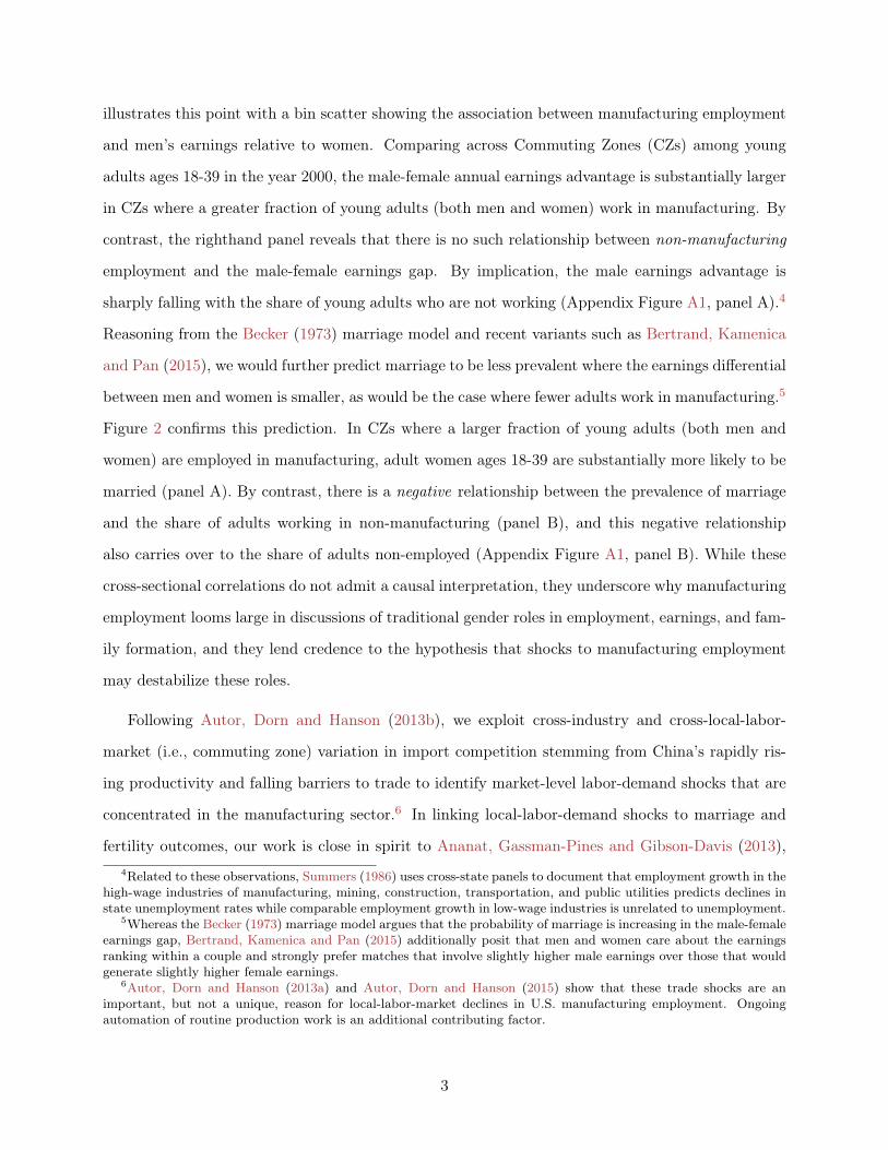
illustrates this point with a bin scatter showing the association between manufacturing employment

and men’s earnings relative to women. Comparing across Commuting Zones (CZs) among young

adults ages 18-39 in the year 2000, the male-female annual earnings advantage is substantially larger

in CZs where a greater fraction of young adults (both men and women) work in manufacturing. By

contrast, the righthand panel reveals that there is no such relationship between non-manufacturing

employment and the male-female earnings gap. By implication, the male earnings advantage is

sharply falling with the share of young adults who are not working (Appendix Figure A1, panel A).4

Reasoning from the Becker (1973) marriage model and recent variants such as Bertrand, Kamenica

and Pan (2015), we would further predict marriage to be less prevalent where the earnings differential

between men and women is smaller, as would be the case where fewer adults work in manufacturing.5

Figure 2 confirms this prediction. In CZs where a larger fraction of young adults (both men and

women) are employed in manufacturing, adult women ages 18-39 are substantially more likely to be

married (panel A). By contrast, there is a negative relationship between the prevalence of marriage

and the share of adults working in non-manufacturing (panel B), and this negative relationship

also carries over to the share of adults non-employed (Appendix Figure A1, panel B). While these

cross-sectional correlations do not admit a causal interpretation, they underscore why manufacturing

employment looms large in discussions of traditional gender roles in employment, earnings, and fam-

ily formation, and they lend credence to the hypothesis that shocks to manufacturing employment

may destabilize these roles.

Following Autor, Dorn and Hanson (2013b), we exploit cross-industry and cross-local-labor-

market (i.e., commuting zone) variation in import competition stemming from China’s rapidly ris-

ing productivity and falling barriers to trade to identify market-level labor-demand shocks that are

concentrated in the manufacturing sector.6 In linking local-labor-demand shocks to marriage and

fertility outcomes, our work is close in spirit to Ananat, Gassman-Pines and Gibson-Davis (2013),4Related to these observations, Summers (1986) uses cross-state panels to document that employment growth in the

high-wage industries of manufacturing, mining, construction, transportation, and public utilities predicts declines instate unemployment rates while comparable employment growth in low-wage industries is unrelated to unemployment.

5Whereas the Becker (1973) marriage model argues that the probability of marriage is increasing in the male-femaleearnings gap, Bertrand, Kamenica and Pan (2015) additionally posit that men and women care about the earningsranking within a couple and strongly prefer matches that involve slightly higher male earnings over those that wouldgenerate slightly higher female earnings.

6Autor, Dorn and Hanson (2013a) and Autor, Dorn and Hanson (2015) show that these trade shocks are animportant, but not a unique, reason for local-labor-market declines in U.S. manufacturing employment. Ongoingautomation of routine production work is an additional contributing factor.

3

Figure 2: Bin-Scatter of the Commuting Zone Level Relationship Between the Manufacturing Em-ployment Share (panel A), the Non-Manufacturing Employment Share (panel b) and the Share ofWomen that Are Currently Married: Adults Age 18-39 in 2000

.4.4

5.5

.55

.6Sh

are

of W

omen

Age

18-

39 C

urre

ntly

Mar

ried

0 .1 .2 .3Share of Population Age 18-39 Employed in Manufacturing

.4.4

5.5

.55

.6Sh

are

of W

omen

Age

18-

39 C

urre

ntly

Mar

ried

.4 .5 .6 .7 .8Share of Population Age 18-39 Employed in Non-Manufacturing

Notes: See Figure 1.

Kearney and Wilson (2016), Schaller (forthcoming 2016), and Shenhav (2016).7 We exploit gender

dissimilarities in industry specialization to identify demand shocks that distinctly affect men’s and

women’s employment and earnings. Our use of trade shocks as a source of variation further allows us

to assess whether two decades of contracting U.S. manufacturing employment in labor-intensive sec-

tors, stemming in substantial part from rising international competition from China, has contributed

to the rapid, simultaneous decline of traditional household structures.

We offer a simple conceptual model of marital decision-making under uncertainty based on Kane

and Staiger (1996) that guides the interpretation of the analysis. Less-skilled unmarried women

have a preference for becoming married mothers but face uncertainty about the quality of their

male partners, which is not fully revealed until after conception of a child. Women who strongly

prefer marriage to single-parenthood (to whom we will refer as having traditional preferences) will

curtail both fertility and marriage when high-quality men become scarce rather than risk becoming

pregnant by and then marrying a low-quality man. Women who are willing to exercise the option7Ananat, Gassman-Pines and Gibson-Davis (2013) find that adverse shocks reduce birthrates and sexual activity

among teens—particularly black teens—while increasing the use of contraception and the incidence of abortion.Relatedly, Shenhav (2016) uses gender-specific Bartik shocks and gender differences in occupational choice to predictchanges in relative gender earnings in U.S. states, drawing its empirical strategy in part on an earlier version ofthis paper (Autor et al., 2014a). Shenav’s complementary focus is on the economic independence of women ratherthan the declining marriage-market value of men. Using a strategy similar to Shenhav (2016), Schaller (forthcoming2016) finds that improvements in men’s labor market conditions predict increases in fertility while improvements inwomen’s labor market conditions have the opposite effect. Kearney and Wilson (2016) find that positive shocks tomale earnings do not increase marriage, but do raise fertility and reduce the non-marital birth share.

4

of single-motherhood in the event of a bad draw of a male partner (those with non-traditional

preferences) will curtail marriage but not (necessarily) fertility when high-quality males become

scarce. Because of the asymmetric fertility responses of women who do and do not value the option

of single-motherhood, this framework predicts that marriage is more elastic than fertility to the

supply of high-quality males. A fall in the supply of high-quality males reduces fertility while raising

the fraction of children born out-of-wedlock and living with unmarried mothers.

We apply a large body of harmonized data sources to quantify the link between differential

shocks to male and female labor-market opportunities and marriage and fertility outcomes. We

first show that shocks to manufacturing labor demand, measured at the commuting-zone level, exert

large impacts on men’s relative annual wage-and-salary earnings. Although earnings losses are visible

throughout the earnings distribution, the relative declines in male earnings are largest at the bottom

of the distribution. We estimate that a trade shock that increases CZ-level import penetration by

one percentage point (a ‘unit’ shock)—roughly equal to the decadal average trade shock over the

1990s and 2000s—reduces the male-female annual earnings advantage by 2.2 percent at the median

and by nearly 17 percent at the 25th percentile. It also increases the share of young men in a local

labor market who earn less than women of the same age, race and education.8

Trade shocks reduce the availability and desirability of potentially marriageable young men

along multiple dimensions. The most immediate effect is in populations shifts: a unit rise in Chinese

import penetration reduces the ratio of male to female young adults in a CZ by 1.7 percentage points.

Where are these men going? Following Case and Deaton (2015) and Pierce and Schott (2016b), we

show that trade shocks lead to a differential rise in mortality from drug and alcohol poisoning, liver

disease, diabetes, and lung cancer among young men relative to young women. The proportional rise

in mortality from these causes is substantial: a one-unit shock more than doubles the relative male

death rate from drug and alcohol poisoning. But this effect is not nearly large enough to explain

the differential decline in the young male population, suggesting that other channels are operative,

including migration, homelessness and incarceration. Regarding criminal activity, Deiana (2015),

Feler and Senses (2015), and Pierce and Schott (2016b) find significant increases in property- and

violent-crime and arrests in trade-exposed CZs during the 1990s and 2000s, which plausibly lead8Autor, Dorn and Hanson (2013a) find that trade shocks reduce CZ-level mean earnings and Chetverikov, Larsen

and Palmer (2016) demonstrate that these shocks raise CZ-level earnings inequality, though though they do not studyimpacts on the gender earnings gap.

5

to larger incarceration rates especially for men. The observed rise in the incidence of drug-related

deaths and crime in trade-exposed locations suggests that trade shocks contribute to a variety of

behaviors that diminish the marriage-market value of males that remain in these locations, including

non-lethal substance abuse or illegal activities that do not lead to incarceration.9

We next assess marriage-market consequences. Consistent with earlier work (Blau, Kahn and

Waldfogel, 2000; Elwood and Jencks, 2004), we find that adverse labor-market shocks reduce the

fraction of young women who are currently married, with especially large effects on the youngest

adult women, ages 18-25. More subtly, we find asymmetric marriage-market impacts that depend

upon the source of the shock: adverse shocks to labor demand in male-intensive industries reduce

the prevalence of marriage among young women, whereas analogous shocks to female labor demand

significantly raise the prevalence of marriage. These asymmetric responses are predicted by our con-

ceptual model: negative shocks concentrated on males reduce their marriage-market value, thereby

discouraging both fertility and marriage; negative shocks concentrated on women raise women’s

disutility of single-motherhood, discouraging fertility but encouraging marriage.

Building on these results, we explore outcomes for fertility. Consistent with the general fact

that fertility is pro-cyclical, we document that a one-unit import shock lowers births per thousand

women of ages 20-39 by 3.3 (a 4% decline). But this decline is not uniform across demographic

groups. Fertility among teens and unmarried women falls by proportionately less than fertility

among older and married women, so that the share of births to unmarried and—more sizably—teen

mothers rises. Recent literature hypothesizes that the high U.S. teen birth rate is in substantial part

due to the dearth of economic opportunity facing young non-college women (Kearney and Levine,

2012). Consistent with this hypothesis, we find that adverse shocks to female labor demand increase

the fertility rate among teens, although the fraction of teen and unmarried births declines by as

much as adverse shocks to male labor demand increase these shares. This asymmetry is consistent

with our simple option-value model of fertility: holding women’s economic opportunities constant, a

decline in male earnings spurs some women to curtail both motherhood and marriage while spurring

others to exercise the option of single-headedness (curtailing marriage but not fertility), thus raising

teen and out-of-wedlock birth shares; conversely, holding men’s economic opportunities constant,

a decline in female earnings raises the relative attractiveness of male partners, which encourages9Our perspective is akin to Charles and Luoh (2010) and Caucutt, Guner and Rauh (2016), who interpret the rise

in male incarceration as an adverse shock to the supply of marriageable men.

6

fertility and marriage while single motherhood becomes a less attractive option.

Finally, we examine how these changes in children’s birth circumstances flow into downstream

parental arrangements and child poverty. A one-unit trade shock raises the fraction of children of

ages 0-17 living in poverty by 2.2 percentage points (a 12% increase), reduces the fraction living

in married households by 0.4 percentage points, and spurs a concomitant rise in the share living

in single- and grandparent-headed households. The asymmetric effect of male and female labor

demand shocks seen for marriage and fertility carries over to household structures. Holding female

economic opportunities constant, shocks to male earnings raise the fraction of children living in

single-headed households, suggesting that woman are curtailing marriage by more than childbearing

(i.e., exercising the option of single parenthood). When female earnings fall, however, the share of

children in single-parent households declines steeply. These shifts in household structure contribute

to differential impacts of gender-specific labor demand shocks on child poverty. Adverse shocks to

male and female earnings both increase the poverty rate. However, the direct effect of reduced

male earnings gets exacerbated as it causes a greater concentration of children in single-parent

homes which have an elevated poverty risk; conversely, the direct of effect of lower female earnings

is mitigated by the decline in single motherhood. Whereas male labor-demand shocks raise the

fraction of children living in poverty, female labor-demand shock have no effect.

Our work contributes to two branches of literature. A first explores how marriage and divorce

rates respond to shifts in labor demand or to changes in welfare benefits (Blau, Kahn and Wald-

fogel, 2000; Elwood and Jencks, 2004).10 A second, following Wilson and Neckerman (1986) and

Wilson (1987), asks whether a shrinking the pool of marriageable low-education men has eroded

the incentive for men to maintain committed relationships, curtailed women’s gains from marriage,

and strengthened men’s bargaining position vis-a-vis casual sex, out-of-wedlock childbirth, and non-

custodial parenting (Angrist, 2002; Charles and Luoh, 2010; Edin and Kefalas, 2011; Edin and

Nelson, 2013; LeBlanc, 2003; Lundberg, Pollak and Stearns, 2015). Despite a substantial body of

evidence, it remains a conceptual and empirical challenge to distinguish cause from effect in the

relationship between household structure and labor-market opportunity.11 Current literature does10The literature tends to find that better male labor-market opportunities increase marriage rates, whereas better

female labor-market opportunities decrease marriage rates. The evidence for a discouragement effect of welfare policieson marriage rates is less certain. Changes in welfare policies are however an unlikely explanation for recent declinesin U.S. marriage rates given that the U.S. welfare system has become less generous over the past two decades.

11Bailey and DiPrete (2016) and Greenwood, Guner and Vandenbroucke (forthcoming) review the changing role ofU.S. women in the household and the labor market, with the former focusing on educational gender norms and skills

7

not offer tightly identified results delineating whether reductions in the supply of ‘marriageable’ men

are in any meaningful sense responsible for the dramatic changes in marriage and out-of-wedlock

fertility observed in the U.S. population. We provide such evidence to the debate.

2 Conceptual Underpinnings

We consider a setting where unmarried women have a preference to become married mothers but face

uncertainty about the availability of high-quality men who may serve as marital partners.12 A sub-

stantial literature documents that the marriage decision tends to follow the fertility decision: upon

becoming pregnant, a woman may choose to marry the child’s father but absent pregnancy would

not elect marriage.13 We impose this setting on decision-making by assuming that women choose

to remain childless, to have a child and marry, or to become a single mother. Removing the option

of marriage without children narrows the generality of the model but is not restrictive empirically

since nearly 90% of women ages 18-39 are either mothers, or unmarried without children.14

Suppose that at the time of considering motherhood, women are uncertain whether the potential

father is a high-quality parent, as father quality is not revealed until after pregnancy has occurred.

Women who choose pregnancy face two options at the time that partner quality is revealed: those

who find that their partners are high-quality will elect marriage; those who find that their partners

are low-quality will choose either to marry their low-quality partners or to raise their children out-of-

wedlock, whichever has greater utility. In this setting, an inward shift in the supply of high-quality

men unambiguously reduces marriage and fertility. Simultaneously, this supply shift may increase

the fraction of births that are out of wedlock and hence the share of children raised in single-headed

households. The intuition, formalized below, is as follows: for women who are committed to raising

development and the latter focusing on technological progress as drivers of these changes. Neither considers the roleof the supply of high-quality males in determining women’s fertility and marriage decisions.

12Our conceptual framework is adapted from Kane and Staiger (1996), who analyze the interaction between abortionrestrictions, fertility, and out-of-wedlock births. In related work, Akerlof et al. (1996) consider how women’s forward-looking decisions about sexual intercourse and marital pre-commitment are shaped by their outside options, whichmay include abortion, in the event of pregnancy. We abstract from the option of abortion in the model and in oursubsequent empirical analysis (it is not observed in our data).

13Edin and Tach (2012) calculate that among women currently over the age of 24 in 2006 through 2008, 53% weremothers by the age of 24, and 65% of those mothers were unmarried at the time of their first birth. Seventy-sixpercent of first births in 2007 were to mothers under the age of 30, and 46% were to women under the age of 25(Martin et al., 2010, Table 3).

14The share of women age 18-39 who are married but have no children declined from 12.5% to 10.2% from 1990to 2007 in Census/ACS data. This demographic status is less prevalent than any other combination of marital andmotherhood status—married with children (decline from 40.6% to 31.9%), unmarried and childless (increase from34.3% to 42.9%), and unmarried with children (increase from 12.7% to 15.0%).

8

children in wedlock—that is, who have high disutility of non-marital childrearing whom we refer

to as having traditional preferences—a decline in the availability of high-quality males deters both

pregnancy and marriage. For women who have a comparatively low psychic cost of non-marital

childrearing (non-traditional preferences), a shrinking pool of high-quality men deters fertility by

less than it deters marriage, shifting the composition of fertility towards non-marital births.

Formally, let potential male partners be either high or low-quality, where quality denotes ability

to provide economic and emotional inputs for parenting that are valued by the mother. At a given

point in time t, a fraction P

ij

of the potential partners for a woman i in commuting zone j are

high-quality while 1 � P

ij

are of low-quality. The expectation of Pij

is common knowledge, but a

woman cannot verify the quality of an individual male partner until she conceives a child with that

partner. We normalize the utility of not having a child at zero and the utility of having a child with

a high-quality father at one, and we assume that women maximize expected utility. The utility for

woman i of marrying a low-quality father is �M

i

, while her utility of raising a child out of wedlock

is �S

i

, with M

i

, S

i

> 0 for all i. The variables P

ij

,M

i

and S

i

can all very according to a women i’s

individual tastes or demographic characteristics.

Labor-market conditions in commuting zone j will affect women’s choices by changing the fraction

P

ij

of men that are perceived to be attractive partners. A negative shock to labor demand for males

reduces the proportion of high-quality male partners P

ij

in the local labor market, while a negative

shock to female labor demand increases P

ij

, as a set of males with a given income level looks more

attractive to women whose own earnings are low. The general premise that higher relative earnings

of males make them more attractive partners is consistent with a long literature going back to

Becker (1973). The more specific and simplifying assumption that male quality depends (in part)

on male relative earnings relates to recent work by Bertrand, Kamenica and Pan (2015) who argue

that potential partners have a strong preference for matches in which the man’s earnings exceed the

woman’s, eschewing matches that combine a higher-earning women with a lower-earning male. In

this setting, a woman will choose to conceive a child if

P

ij

1� P

ij

> min [Mi

, S

i

] ,

that is, if the odds that her partner is revealed to be high-quality after conception are sufficiently

high to overcome the risk that she will have to marry a low-quality father (if Mi

S

i

) or become a

9

single mother (if Mi

> S

i

) .

Figure (3) illustrates the operation of this simple model. The y�axis of the figure corresponds to

P

ij

, the probability that a male partner will be revealed to be of high quality following conception.

The x�axis corresponds to the disutility of single-motherhood, Si

. For concreteness, we depict the

preferences of women who have a given level of disutility M

i

of marrying a low-quality father.

Figure 3: Women’s Choices Over Pregnancy, Marriage and Single-Motherhood as a Function ofExpected Male Quality (P

ij

) and Disutility of Single Motherhood (Si

) for a Given Level of Disutilityof Marrying a Low-Quality Male (M

i

)

0

1

0 2

Pro

ba

bili

ty t

ha

t P

art

ne

r is

a H

igh

Qu

alit

y F

ath

er,

P

Womenwith non-traditionalpreferencesaredeterredfromchildbearingbylow!"# inthisregion

Disutility of Single Motherhood, $"

min $"1 + $"

, ,"1 +,"

,"1 + ,"

,"

Region1

Non-Mothers:ExpectedCostsofPregnancyExceed

ExpectedBenefits

Pr /ℎ123 = 0Pr ,677183 = 0Pr $19:28,;<ℎ87 = 0

Region2

MotherswithTraditionalPreferences:DisutilityofSingleMotherhood ExceedsDisutilityofMarriagetoLowQMale

Pr /ℎ123 = 1Pr ,677183 = 1Pr $19:28,;<ℎ87 = 0

Region3

MotherswithNon-TraditionalPreferences:DisutilityofMarriagetoLowQMale

ExceedsDisutilityofSingleMotherhood

Pr /ℎ123 = 1Pr ,677183 = !"#Pr $19:28,;<ℎ87 = 1 −!"#

Womenwith traditionalpreferencesaredeterredfromchildbearingbylow!"# inthisregion

Region 1 in the figure depicts the area in which P

ij

< min⇣

Si1�Si

,

Mi1�Mi

⌘. In this region, women

will choose against motherhood because the probability that a father proves to be high-quality are

too small to overcome the downside risk of either marrying a low-quality father (�M

i

) or raising

a child as a single mother (�S

i

).15 Region 2 captures women for whom the disutility of single-

motherhood exceeds the disutility of marrying a low-quality father (�S

i

< �M

i

) and for whom

15Note that the condition for fertility, Pij

1�Pij> min (Si,Mi), can be rewritten as Pij > min

⇣Si

1�Si, Mi1�Mi

⌘.

10

the benefits of pregnancy exceed the downside risk. Women with these traditional preferences will

choose motherhood and will marry the child’s father whether or not he is ultimately revealed to be

of high or low quality. Region 3 depicts the set of women for whom single-motherhood is preferable

to marrying a low-quality father (�M

i

< �S

i

) and for whom the benefits of pregnancy exceed the

downside risk of raising a child out of wedlock. Women with these non-traditional preferences will

choose motherhood but will marry the child’s father only if he is revealed to be high-quality.

Consider the effects on fertility and marriage of a shock in commuting zone j that worsens the

labor-market opportunities for males, thus reducing the local supply of high-quality fathers (a drop

in P

ij

). Among women with traditional preferences (right half of the figure), outcomes are unchanged

with the decline in P

ij

for those women who remain in either Region 1 or Region 2. For some women,

however, Pij

falls below M

i

/ (1�M

i

) and pushes them from Region 2 into Region 1, where they

abstain from both motherhood and marriage. Thus, for women with traditional preferences, the

probability of motherhood and marriage falls in lockstep.

Women with non-traditional preferences (left half of the figure) face a more complex choice set

since single-motherhood provides option value should the father of the child prove to be low-quality.

A first group is already initially in Region 1 and continues to forgo motherhood and marriage as

the quality of potential spouses deteriorates. A second group moves from Region 3 to Region 1

as P

ij

falls below S

i

/ (1� S

i

), and thus abstains from both fertility and marriage. Finally, a third

group of women with non-traditional preferences remains in Region 3 as P

ij

continues to be larger

than S

i

/ (1� S

i

). These women will not adjust fertility, but as they prefer single-motherhood to

marrying a low-quality father, their marriage rate declines as the supply of high-quality males falls.

In combination, the adjustments among women with traditional and non-traditional preferences

sum to an unambiguously negative impact of a deterioration in male partner quality on both fertility

(by shifting women from Regions 2 and 3 to Region 1) and marriage (by shifting women into Region

1 and reducing marriage rates within Region 3). Under mild additional assumptions, marriage rates

will fall more than fertility, thus increasing the fraction of out-of-wedlock births. Intuitively, the

shift of women into Region 1 has modest implications for the rate of single motherhood among the

remaining mothers, as it reduces both the number of traditional mothers who are always married

and the number of marginal non-traditional mothers who are mostly single. The main impact of the

economic shock on single motherhood thus operates via the declining likelihood of marriage among

11

mothers with non-traditional preferences (those who remain in Region 3).16

Consider next the comparative statics for a shock in commuting zone j that reduces labor-market

opportunities for women, raises the relative earnings of males, and thus increases the likelihood that

males will be perceived as being of high quality (an increase in P

ij

). The shift of women from Region

1 to Regions 2 and 3 increases both fertility and the number of marriages. In addition, women in

Region 3 become more likely to choose marriage over single motherhood, and contrary to the impact

of a shock to male labor demand, the share of out-of-wedlock births is thus likely to decline. Thus,

opposite to the case of adverse shocks to relative male earnings, adverse shocks to relative female

earnings are likely to increase transitions into marriage by more than transitions into motherhood.

Despite its simplicity, this framework encapsulates a broadly applicable insight: women must

make forward-looking, irreversible fertility decisions in a setting where the consequences of preg-

nancy—father quality in particular—are uncertain until at least the time that the child is conceived.

Facing the possibility of obtaining a low-quality partner, women’s outside options play a critical

role in determining their willingness to risk childbearing. This simple framework offers a number of

predictions that we subsequently test and confirm:

1. Adverse shocks to male earnings capacity: (a) reduce overall fertility and the prevalence of mar-

riage, and (b) reduce marriages by more than births (because some women with non-traditional

preferences chose to become single mothers rather than marrying low-quality males), thereby

increasing the share of children born out-of-wedlock and raised in single-headed households;

2. Adverse shocks to women’s earnings capacity: (a) increase overall fertility and marriage rates,

and (b) increase marriages more than births, thus decreasing the share of children born out-16More formally, denote by m the probability that a women has traditional preferences, by b the fraction of tradi-

tional women that choose motherhood both before or after a given shock �Pij < 0, and by � the fraction of traditionalwomen that would become mothers only absent the shock, while a and ↵ correspondingly denote the fractions of non-traditional women who would choose motherhood regardless of the shock, or only absent the shock. Finally, p and ⇡ arethe average pre-shock marriage rates for the two groups of non-traditional women who become mothers either regard-less of the shock or only absent the shock. The shock �Pij < 0 increases the share of out-of-wedlock births if it causes agreater relative decline in married mothers than in single mothers, (�m� � (1�m)↵) / (m(b+ �) + (1�m)(a+ ↵)) <(�a(1� ⇡)� a�Pij) (a(1� p) + ↵(1� ⇡)). A sufficient but not necessary condition for this inequality to hold is(1 +m (b/a� 1)) / (1 +m (�/↵� 1)) (1� p) / (1� ⇡), which implies that the combined effect of women movingfrom Regions 2 and 3 to Region 1 in Figure (3) will weakly increase the rate of out-of-wedlock birth among theremaining mothers. Since the probability of single motherhood is smaller for inframarginal than for marginal non-traditional women, (1� p) / (1� ⇡) < 1, this condition requires that the relative shift of traditional women intonon-motherhood is larger than the corresponding shift for non-traditional mothers, �/b > ↵/a. If this condition isnot fulfilled, then the decline in fertility induced by the shock will depress the share of single mothers, but this effectstill trades off against the rise in single motherhood due to the reduced marriage rate within Region 3, thus allowingthe share of single motherhood to rise in the aggregate.

12

of-wedlock and raised in single-headed households.

This model, of course, ignores many salient considerations for fertility and marriage, including

the option for women to seek abortions, and the reality that adults marry for reasons other than

childrearing. Nevertheless, it captures a subtle mechanism by which shocks to male and female

earnings produce distinct effects on fertility, marriage, and the prevalence of single-motherhood.

3 Data and Measurement

3.1 Local labor markets

We approximate local labor markets using the construct of Commuting Zones (CZs) developed

by Tolbert and Sizer (1996). Our analysis includes the 722 CZs that cover the entire mainland

United States (both metropolitan and rural areas). Commuting zones are particularly suitable for

our analysis of local labor markets because they cover both urban and rural areas, and are based

primarily on economic geography rather than incidental factors such as minimum population.17

3.2 Exposure to international trade

Following Autor, Dorn and Hanson (2013b), we examine changes in exposure to international trade

for U.S. CZs associated with the growth in U.S. imports from China. The focus on China is a natural

one: rising trade with China is responsible for nearly all of the expansion in U.S. imports from low-

income countries since the early 1990s. China’s export surge is a consequence of its transition to a

market-oriented economy, which has involved rural-to-urban migration of over 250 million workers

(Li, Li, Wu and Xiong, 2012), Chinese industries gaining access to long banned foreign technologies,

capital goods, and intermediate inputs (Hsieh and Klenow, 2009), and multinational enterprises

being permitted to operate in the country (Naughton, 2007).18 Compounding the effects of internal

reforms on China’s trade is the country’s accession to the World Trade Organization in 2001, which

gives it most-favored nation status among the 157 WTO members (Pierce and Schott, 2016a).17Parts of our analysis draw on Public Use Microdata from Ruggles, Sobek, Fitch, Goeken, Hall, King and Ron-

nander (2004) that indicates an individual’s place of residence at the level of Public Use Micro Areas (PUMAs). Weallocate PUMAs to CZs using the probabilistic algorithm developed in Dorn (2009) and Autor and Dorn (2013).

18While China overwhelmingly dominates low-income country exports to the U.S., trade with middle-income nations,such as Mexico, may also matter for U.S. labor-market outcomes. Hakobyan and McLaren (2016) find that NAFTAreduced wage growth for blue-collar workers in exposed industries and locations.

13

In the empirical analysis, we follow the specification of local trade exposure derived by Autor,

Dorn, Hanson and Song (2014b) and Acemoglu, Autor, Dorn, Hanson and Price (2016). Our measure

of the local-labor-market shock is the average change in Chinese import penetration in a CZ’s

industries, weighted by each industry’s share in initial CZ employment:

�IP

cu

i⌧

=X

j

L

ijt

L

it

�IP

cu

j⌧

. (1)

In this expression, �IP

cu

j⌧

= �M

cu

j⌧

/(Yj0 +M

j0 �X

j0) is the growth of Chinese import penetration

in the U.S. for industry j over period ⌧ , which in our data include the time intervals 1990 to 2000

and 2000 to 2007. Following Acemoglu, Autor, Dorn, Hanson and Price (2016), it is computed as the

growth in U.S. imports from China, �M

cu

j⌧

, divided by initial absorption (U.S. industry shipments

plus net imports, Yj0 +M

j0 � X

j0) in the base year 1991, near the start of China’s export boom.

The fraction L

ijt

/Lit

is the share of industry j in CZ i ’s total employment, as measured in County

Business Patterns data at the start of each period.

In (1), the difference in �IP

cu

it

across commuting zones stems from variation in local industry

employment structure at the start of period t, which arises from differential concentration of employ-

ment in manufacturing versus non-manufacturing activities and specialization in import-intensive

industries within local manufacturing. Importantly, differences in manufacturing employment shares

are not the primary source of variation. In a bivariate regression, the start-of-period manufacturing

employment share explains less than 40 percent of the variation in �IP

cu

it

. In all specifications,

we control for the start-of-period manufacturing share within CZs so as to focus on variation in

exposure to trade stemming from differences in industry mix within local manufacturing.

The measure �IP

cu

i⌧

captures overall trade exposure experienced by CZs but does not distinguish

between employment shocks that differentially affect male and female workers. To add this dimension

of variation to �IP

cu

i⌧

, we modify (1) to account for the fact that manufacturing industries differ

in their male and female employment intensity; hence, trade shocks of a given magnitude will

differentially affect male or female employment depending on the set of industries that are exposed.

We incorporate this variation by multiplying the CZ-by-industry employment measure in (1) by the

initial period female or male share of employment in each industry by CZ (fijt

and 1 � f

ijt

), thus

apportioning the total CZ-level measure into two additive subcomponents, �IP

m,cu

i⌧

and �IP

f,cu

i⌧

:

14

�IP

m,cu

i⌧

=X

j

(1� f

ijt

)Lijt

L

it

�IP

cu

j⌧

and �IP

f,cu

i⌧

=X

j

f

ijt

L

ijt

L

it

�IP

cu

j⌧

, (2)

Concretely, consider the hypothetical example of a CZ that houses two import-competing manufac-

turing industries, leather goods and rubber products, both of which employ the same number of

workers and are exposed to industry-specific import shocks equal to 1 percent of initial domestic

absorption (thus, �IP

cu

i⌧

= 1.0 for this CZ). Imagine that 55 percent of leather goods workers in

the CZ are women while 75 percent of rubber products workers in the CZ are men. Equation (2)

would apportion these industry by commuting zone trade shocks to males and females according

to their local industry employment shares such that �IP

m,cu

i⌧

= 0.45 ⇥ 1.0 + 0.75 ⇥ 1.0 = 0.6 and

�IPW

f

uit

= 0.55 ⇥ 1.0 + 0.25 ⇥ 1.0 = 0.4. In this example, we would assign a larger fraction of a

CZ’s trade shock to males than to females because males constitute a larger fraction of employment

in the CZ’s trade-exposed industries. Although the example is hypothetical, the numbers are quite

close to the data, as shown in Appendix Table A1. For the period of 1990 - 2000, our data indicate

a mean rise of Chinese import penetration of 0.94 percentage points, 60 percent of which accrued

to male employment and 40 percent to female employment. In the subsequent 2000 - 2007 period,

when Chinese import penetration accelerated sharply, import penetration rose by an additional 1.33

percent, with 65 percent of this rise accruing to male employment.

To identify the supply-driven component of Chinese imports, we instrument for growth in Chinese

imports to the U.S. using the contemporaneous composition and growth of Chinese imports in eight

other developed countries.19 Specifically, we instrument the measured import-exposure variable

�IP

cu

it

with a non-U.S. exposure variable �IP

co

it

that is constructed using data on industry-level

growth of Chinese exports to other high-income markets:

�IP

co

it

=X

j

L

ijt�10

L

uit�10�IP

co

j⌧

. (3)

This expression for non-U.S. exposure to Chinese imports differs from the expression in equation

(1) in two respects. In place of computing industry-level import penetration with U.S. imports by

industry (�M

cu

j⌧

), it uses realized imports from China by other high-income markets (�M

co

j⌧

), and it

replaces all other variables with lagged values to mitigate any simultaneity bias.20 As documented by19The eight other high-income countries are those that have comparable trade data covering the full sample period:

Australia, Denmark, Finland, Germany, Japan, New Zealand, Spain, and Switzerland.20The start-of-period employment shares Lijt/Lit and the gender shares fijt are replaced by their 10 year lags,

while initial absorption in the expression for industry-level import penetration is replaced by its 3 year lag.

15

Autor, Dorn and Hanson (2016), all eight comparison countries used for the instrumental variables

analysis witnessed import growth from China in at least 343 of the 397 total set of manufacturing

industries. Moreover, cross-country, cross-industry patterns of imports are strongly correlated with

the U.S., with correlation coefficients ranging from 0.55 (Switzerland) to 0.96 (Australia). That

China made comparable gains in penetration by detailed sector across numerous countries in the

same time interval suggests that China’s falling prices, rising quality, and diminishing trade and

tariff costs in these surging sectors are a root cause of its manufacturing export growth.21

The exclusion restriction underlying our instrumentation strategy requires that the common

component of import growth in the U.S. and in other high income countries derives from factors

specific to China, associated with its rapidly evolving productivity and trade costs. Any correlation

in product demand shocks across high income countries would represent a threat to our strategy,

possibly contaminating both our OLS and IV estimates.22 To check robustness against correlated

demand shocks, Autor, Dorn and Hanson (2013a) develop an alternative estimation strategy based

on the gravity model of trade. They regress China exports relative to U.S. exports to a common

destination market on fixed effects for each importing country and for each industry. The time

difference in residuals from this regression captures the percentage growth in imports from China

due to changes in China’s productivity and foreign trade costs vis-a-vis the U.S. By using China-

U.S. relative exports, the gravity approach differences out import demand in the purchasing country,

helping to isolate supply and trade-cost driven changes in China’s exports. These gravity-based

estimation results are quite similar to the IV approach that we employ in this paper.23

Data on international trade are from the UN Comtrade Database, which gives bilateral imports

for six-digit HS products.24 To concord these data to four-digit SIC industries, we apply the cross-

walk in Pierce and Schott (2012), which assigns ten-digit HS products to four-digit SIC industries21A potential concern about our analysis is that we largely ignore U.S. exports to China, focusing instead on trade

flows in the opposite direction. This is for the simple reason that our instrument, by construction, has less predictivepower for U.S. exports to China. Nevertheless, to the extent that our instrument is valid, our estimates will correctlyidentify the direct and indirect effects of increased import competition from China. We note that imports from Chinaare much larger—approximately five times as large—as manufacturing exports from the U.S. to China. To a firstapproximation, China’s economic growth during the 1990s and 2000s generated a substantial shock to the supply ofU.S. imports but only a modest change in the demand for U.S. exports.

22Note that positive correlation in product demand shocks across high-income economies would make the impactof trade exposure on labor-market outcomes appear smaller than it truly is since these shocks would generate risingimports and rising domestic production simultaneously.

23See Autor, Dorn and Hanson (2013a) and Autor, Dorn, Hanson and Song (2014b) for further discussion of possiblethreats to identification using our instrumentation approach, and see Bloom, Draca and Van Reenen (2015) and Pierceand Schott (2016a) for alternative instrumentation strategies for the change in industry import penetration.

24See http://comtrade.un.org/db/default.aspx.

16

(at which level each HS product maps into a single SIC industry), and aggregate up to the level of

six-digit HS products and four-digit SIC industries (at which level some HS products map into mul-

tiple SIC entries). To perform this aggregation, we use data on U.S. import values at the ten-digit

HS level, averaged over 1995 to 2005. All dollar amounts are inflated to dollar values in 2007 using

the PCE deflator. Data on CZ employment by industry from the County Business Patterns for 1990

and 2000 is used to compute employment shares by 4-digit SIC industries in (1) and (3).25

4 The Supply of Marriageable Males

We begin by assessing whether trade shocks curtail the supply of marriageable males under age 40,

as measured by their employment and absolute and relative earnings, physical availability in trade-

impacted labor markets, and participation in risky and damaging behaviors. Across all margins,

we find unambiguous evidence that adverse labor-market shocks stemming from trade exposure,

whether measured in aggregate or disaggregated by gender, curtail the supply of young men who

would likely be judged as good marital prospects.

4.1 Employment effects

The trade shocks that form the basis for our identification strategy are concentrated in manufactur-

ing. We thus set the stage by characterizing the role that manufacturing plays in the employment

of young adults. In 1990, 17.4 percent of men and 8.7 percent of women ages 18-39 worked in

manufacturing. Focusing only on those currently employed, these shares were 21.8 percent and 12.9

percent respectively—that is, more than one in five young male workers and more than one in eight

young female workers. These shares fell substantially in the ensuing two decades. By 2007, only

10.9 percent of men and 4.6 percent of women ages 18-39 worked in manufacturing (14.1 and 6.8

percent among those currently employed), corresponding to a fall of more than 35 percent among

young men and more than 45 percent among young women.26

Although declining manufacturing employment was largely offset by gains in non-manufacturing

employment—in net, employment-to-population fell by 2.0 percentage points among men and by25Because Census industry categories are somewhat coarser than the SIC codes available in the Country Business

Patterns data from which we calculate CZ-by-industry employment, we assign to each SIC industry in a CZ the gendershare of the Census industry in the CZ encompassing it when calculating gender-specific employment shocks.

26These calculations are based on our main Census of populations samples discussed further below.

17

roughly zero among women—the sectoral shift away from manufacturing may nonetheless be conse-

quential for marriage and fertility outcomes if manufacturing jobs provide superior hourly earnings

or annual hours than non-manufacturing jobs. Descriptive regressions reported in Appendix Table

A2 strongly suggest that this is the case. Controlling for an extensive set of covariates, including

detailed indicators for age, education, race, nativity, and a complete set of CZ main effects, we

estimate that annual earnings of men and women age 18-39 working in manufacturing are approxi-

mately 20 log points higher than annual earnings of demographically comparable adults working in

non-manufacturing in the year 2000. Approximately 60 percent of this annual earnings differential

is attributable to higher annual hours among manufacturing workers, with the remaining 40 percent

attributable to higher hourly earnings.27 Although these cross-sectional comparisons may overesti-

mate the causal effect of manufacturing employment on annual earnings despite detailed controls

for observable worker characteristics, they are in line with an established literature that documents

large industry wage premia in manufacturing (Krueger and Summers, 1988). The wage premia for

male and female workers are similar in percentage terms, but larger for males in absolute value due

to the overall higher wage level for males. The sectoral shift out of manufacturing may thus have

eroded earnings especially for males, not only because men make up a disproportionate share of the

sector’s workforce, but also because the average male manufacturing job has a larger dollar wage

premium than the average female manufacturing job.

We assess the causal effect of trade shocks on employment by fitting models of the form

�Y

sit

= ↵

t

+ �1�IP

cu

it

+X0it

�2 + e

sit

, (4)

where �Y

sit

is the decadal change in the manufacturing employment share of the young adult

population ages 18 - 39 in commuting zone i among gender group s (males, females, or both)

during time interval t, calculated using Census IPUMS samples for 1990 and 2000 (Ruggles, Sobek,

Fitch, Goeken, Hall, King and Ronnander, 2004), and pooled American Community Survey samples

for 2006 through 2008. Our focus is on employment of young adults because this population is

disproportionately engaged in marriage and child-rearing.28 We estimate (4) separately for the 1990s27In untabulated results, we find that among men age 18-39 employed in manufacturing in 2000, 35% were in the

top quartile of unconditional male annual wage and salary earnings in their commuting zone, another 33% were inthe second quartile, and 32% were in the bottom two quartiles. The distribution of earnings in manufacturing wassimilarly skewed towards upper quartiles for women.

28Our sample is further restricted to individuals who are not residents of institutionalized group quarters such asprisons, and who are thus potential participants in the local labor and marriage markets.

18

and 2000s, and subsequently stack the ten-year equivalent first differences for 1990 to 2000 and 2000

to 2007, while including time dummies for each decade (in ↵

t

). The explanatory variable of interest

in this estimate is the change in CZ-level import exposure �IP

cu

it

, which in most specifications is

instrumented by �IP

co

it

as described above. When we turn to gender-specific estimates, we replace

�IP

cu

it

with �IP

m,cu

it

and �IP

f,cu

it

, and use the corresponding gender-specific instruments. The

control vector X0it

contains a set of start-of-period CZ-level covariates detailed below.

Table 1: OLS and 2SLS Estimates of the Relationship between Import Penetration and CZ-LevelManufacturing Employment, 1990-2007. Dependent Var: 100 x Change in Share of Population Age18-39 Employed in Manufacturing (in % pts)

OLS OLS OLS 2SLS 2SLS1990-’00 2000-’07 1990-’07 1990-’00 2000-’07

(1) (2) (3) (4) (5)

-0.65 * -1.85 ** -1.44 ** -2.14 ** -2.54 **

(0.27) (0.14) (0.17) (0.43) (0.18)

2SLS First Stage Estimate n/a n/a n/a 0.73 ** 0.86 **

(0.06) (0.06)

R2 0.33 0.62

(6) (7) (8) (9) (10)

-2.44 ** -2.64 ** -2.33 ** -2.32 ** -2.52 **

(0.20) (0.35) (0.34) (0.36) (0.40)

Manufacturing Emp Share-1 Yes Yes Yes YesCensus Division Dummies Yes Yes YesOccupational Composition-1 Yes YesPopulation Composition-1 Yes

2SLS First Stage Estimate 0.82 ** 0.60 ** 0.62 ** 0.60 ** 0.59 **

(0.05) (0.05) (0.05) (0.05) (0.06)

R2 0.55 0.60 0.61 0.63 0.63Notes: N=722 in columns 1-2 and 4-5, N=1444 (722 commuting zones x 2 time periods) in columns 3 and 6-10. All stacked first differences regressions in column 3 and 6-10 include a dummy for the 2000-2007 period. Occupational composition controls in columns 9-10 comprise the start-of-period indices of employment in routine occupations and of employment in offshorable occupations as defined in Autor and Dorn (2013). Population controls in column 10 comprise the start-of-period shares of commuting zone population that are Hispanic, black, Asian, other race, foreign born, and college educated, as well as the fraction of women who are employed. Robust standard errors in parentheses are clustered on state. Models are weighted by start of period commuting zone share of national population. ~ p ≤ 0.10, * p ≤ 0.05, ** p ≤ 0.01.

Δ Chinese Import Penetration

2SLS: 1990-’07

Δ Chinese Import Penetration

The first panel of Table 1 presents initial results. As a point of comparison, the first two columns

19

report OLS estimates of (4) and contain no covariates aside from a constant. Consistent with Autor,

Dorn and Hanson (2013a), we find a negative association between rising Chinese import penetration

and declining U.S. manufacturing employment in exposed CZs. The highly significant coefficients

of �0.65 and �1.85 in columns 1 and 2 indicate that each percentage point rise in import exposure

faced by a CZ is associated with a fall of approximately 0.7 points in the share of non-elderly adults

employed in manufacturing during the 1990s, and a corresponding fall of 1.9 points for the 2000s.

Column 3 stacks these two first differences, yielding an OLS point estimate of �1.44.

Because observed variation in Chinese import penetration includes both China-based supply

shocks—which will tend to reduce competing domestic employment—and domestic demand shocks

for specific goods—which will tend to increase both imports and U.S. manufacturing employment

simultaneously—we would expect OLS estimates of the relationship between import penetration

and domestic employment to be biased towards zero, that is, understating the causal effect of an

exogenous increase in import supply on U.S. manufacturing. Columns 4 and 5 of Table 4, which

employ our instrumental variables strategy, confirm this expectation. We find that each percentage-

point rise in import penetration causes a decline in U.S. manufacturing employment per working-age

population of �2.1 points in the 1990s and �2.5 points in the 2000s. These coefficients are precisely

estimated, as are the first-stage coefficients reported at the bottom of each column. The second set

of five columns in Table 1 refine our approach and test robustness. Column 6 performs a stacked

first-difference estimate, yielding a point estimate of �2.44. Columns 7 through 10 cumulatively

add a rich vector of controls (Xit

in equation 4) to account for factors that might independently

affect manufacturing employment: the lagged share of CZ employment in manufacturing, absorbing

any general shock to manufacturing that leads to a proportional contraction of the sector (column

7); Census division dummies, allowing for regional employment trends (column 8); occupational

composition controls, accounting for employment in occupations susceptible to automation and

offshoring (column 9); and measures of CZ demographics, including race, education, and the fraction

of working-age adult women who are employed, which may affect labor supply to manufacturing

(column 10).29 These controls, which we include in all subsequent regressions, have negligible effects29Occupational controls in column 9 include, first, the fraction of employment in routine task-intensive occupations,

which numerous papers find is a strong predictor of machine-displacement of labor in codifiable clerical, administrativesupport, production and operative tasks (Autor and Dorn, 2013; Goos, Manning and Salomons, 2014; Michaels, Natrajand Van Reenen, 2014), and second, the mean index of ‘offshorability’ for occupations in a CZ, where occupationsare coded as offshorable if they do not require either direct interpersonal interaction with customers or proximity toa specific work location. Population controls in column 10 comprise the start-of-period shares of CZ population that

20

on the magnitude and the precision of the impact estimate. We estimate in the final column that a

one percentage point rise in import penetration in a CZ causes a �2.52 percentage point change in

CZ manufacturing employment as a share of adult population.30

How large are these effects? One benchmark is to scale the impact estimate by the interquartile

range of rising import exposure across CZs during this time period, equal to 0.74 percentage points

per decade (Appendix Table A1). Multiplying the IQR by the column 10 impact estimate of �2.52

implies that rising trade exposure reduced manufacturing employment by 1.9 percentage points more

per decade in CZs at the 75th percentile of exposure relative to those at the 25th percentile of exposure.

As another comparison, the mean per-decade increase in CZ exposure was 1.13 percentage points,

implying that the mean CZ lost 3.35 additional percentage points of manufacturing employment per

decade relative to a CZ with no exposure. These magnitudes are sizable: only 13.0 percent of young

adults age 18-39 were employed in manufacturing in 1990, and this fraction fell by 3.1 percent per

decade over the next seventeen years (bottom row Table 2).

The next set of results estimates the consequences of trade shocks on various employment and

non-employment outcomes by sex—manufacturing employment, non-manufacturing employment,

unemployment, and non-participation—and implements the gender-specific instrumental variables

strategy described above. For comparison, column 1 of the upper panel of Table 2 replicates the

final estimate from Table 1 that includes the full set of covariates that now constitute the base-

line specification. The next two columns estimate the impact of trade exposure on manufacturing

employment among young men and young women, separately. The point estimates of �2.60 and

�2.40 for men and women respectively indicate that the trade shocks seen in this time period had

comparable impacts on manufacturing employment rates of both sexes—though the proportional

impact for women was larger since roughly twice as large a share of young men as young women was

employed in manufacturing at the start of the period (bottom row Table 2).

The lower panel of Table 2 augments these specifications to include male- and female-specific

trade exposure measures, each instrumented by contemporaneous changes in China’s import pene-

are Hispanic, black, Asian, other race, foreign born, and college educated, as well as the fraction of women who areemployed.

30Autor, Dorn and Hanson (2013a) adjust this estimate downward by half to account for the fact that only about50 percent of the rise in U.S. exposure to Chinese imports during this period can be directly attributed to importsupply shocks via the identification strategy described above. We provide rough benchmark numbers here since ourobjective is to characterize the effect of employment shocks on marriage and household structure, and not to accountfor aggregate trends in U.S. manufacturing.

21

tration to other high income countries during. Despite the relatively high correlation between the

gender-specific shock measures (⇢ = 0.82), there is abundant statistical power for distinguishing

their independent effects on labor-market outcomes. The first set of estimates in the lower panel

indicate that a one-percentage point rise in import penetration of either male or female-dominated

industries reduces young adult manufacturing employment by approximately 2.5 percentage points,

as suggested by the by-sex estimates in the upper panel. Columns 2 and 3 demonstrate that the

employment effects of sex-specific shocks—constructed by interacting import exposure with gender

shares of CZ-by-industry employment—fall almost entirely on their corresponding genders. A one-

percentage-point import-penetration shock to male-specific industries reduces employment of young

males in manufacturing by 5.0 percentage points (t = �4.2) and has a small and statistically insignif-

icant impact on female manufacturing employment.31 Conversely, a one-percentage-point shock to

female-specific industries reduces employment of young women in manufacturing by 5.9 percentage

points (t = �5.1), while having no measurable effect on male manufacturing employment. The

fourth column in Table 2 combines these sex-specific outcomes by using as the dependent variable

the male-female difference in manufacturing employment. It shows that a one-percentage-point rise

in male-specific import penetration reduces the male-female manufacturing employment differential

by 5.1 percentage points while a corresponding shock to female-specific import penetration raises

this differential by 6.9 percentage points.32

Columns 5 through 8 provide a regression-based decomposition of how shocks to male-female

differential in manufacturing employment net out across three other domains: non-manufacturing

employment, unemployment, and non-participation, where each outcome is measured for young

adults ages 18 - 39. Due to their common scaling, the net effect of the trade shock must be zero

across these four exhaustive and mutually exclusive domains. The first row of estimates in the

lower panel reveals that fully half of the fall in male relative to female manufacturing employment

induced by the male shock (2.6 of 5.1 percentage points) accrues to a rise in male relative to female31We use the terms male-specific and female-specific shocks as a shorthand for the gender-specific trade exposure

measure as defined in(2). In reality, industries are not specific to one gender, but the sex composition of manufacturingemployment does vary substantially across industries, CZs and industry-CZ pairs.

32Note that the column 4 coefficient for the effect of the male-specific shock on the male-female difference inmanufacturing employment is equal by construction to the difference between the male-specific shock coefficients incolumns 2 and 3 for male and female manufacturing employment separately (�5.03� 0.02 = �5.05), while a parallelequality holds for the female-specific shock coefficient in column 4 (0.94 � (�5.02) = 6.86). Since the overall tradeshock in the upper panel of the table reduces manufacturing employment almost evenly among males and females,it has only a modest impact on the male-female manufacturing employment differential (�2.60 � (�2.40) = �0.19,using rounded numbers).

22

non-manufacturing employment, while another 45% (2.3 of 5.1 percentage points) accrues to a rise

in male relative to female non-participation (not in the labor force, abbreviated as NILF), with the

remaining 5% accruing to a rise in the male-female unemployment gap. Thus, each one-point trade-

induced fall in male relative to female manufacturing employment yields a half point net reduction

in male relative to female labor-force participation. The second row of estimates documents parallel

findings for female-specific trade shocks: 40% of the reduction in female relative to male employment

in manufacturing accrues to rising female relative to male employment in non-manufacturing, while

55% accrues to non-participation, with only 5% to unemployment. These results are consistent with

Autor and Dorn (2013) and Autor, Dorn, Hanson and Song (2014b), who document that adverse

shocks to manufacturing employment are only partially offset by sectoral mobility, leading to large

net reductions in employment. What these results add is a well-identified gender-specific dimension

to employment shocks, which is crucial for the analysis that follows.

Table 2: 2SLS Estimates of the Impact of Import Penetration on Employment Status by Gender,1990-2007. Dependent Var: 100 x Change in Share of Overall/Male/Female Population Age 18-39Employed in Manufacturing (in % pts); 100 x Change in Male-Female Differential in Fraction ofPopulation Age 18-39 that is Employed, Unemployed or Non-Employed (in % pts)

All Males Females Mfg Non-Mfg Unemp NILF(1) (2) (3) (4) (5) (6) (7)

-2.52 ** -2.60 ** -2.40 ** -0.19 0.41 0.04 -0.26(0.40) (0.47) (0.36) (0.29) (0.34) (0.17) (0.34)

-2.51 ** -5.03 ** 0.02 -5.05 ** 2.61 * 0.19 2.26 *(0.87) (1.20) (0.74) (0.98) (1.09) (0.44) (0.97)

-2.54 * 0.94 -5.92 ** 6.86 ** -2.77 * -0.18 -3.91 **(1.10) (1.39) (1.16) (1.37) (1.31) (0.58) (1.32)

Mean Outcome Variable -3.13 -3.86 -2.48 -1.38 -0.03 -0.06 1.46Level in 1990 12.98 17.37 8.68 8.69 3.59 1.22 -13.50

Δ Chinese Import Penetration × (Female Ind Emp Share)

Notes: N=1444 (722 CZ x 2 time periods). All regressions include the full vector of control variables from Table 1. Robust standard errors in parentheses are clustered on state. Models are weighted by start of period commuting zone share of national population. ~ p ≤ 0.10, * p ≤ 0.05, ** p ≤ 0.01. ~ p ≤ 0.10, * p ≤ 0.05, ** p ≤ 0.01.

I. Overall Trade Shock

Δ Chinese Import Penetration

B. Male-Female Differential by Employment Status

A. Share Pop Age 18-39 in Manufacturing

II. Male Industry vs Female Industry Shock

Δ Chinese Import Penetration × (Male Ind Emp Share)

23

4.2 Relative earnings

In this section, we estimate the effect of trade shocks on quantiles of the gender gap in the earnings

distribution in local labor markets. The conceptual model in Section 2 emphasizes the central role

of the gender earnings gap in determining marriage market and fertility outcomes. Shocks that

compress the gender earnings differential in a local market reduce the attractiveness of men as

potential spouses, thus reducing fertility and especially marriage rates. The trade-induced decline

in manufacturing employment may contribute to a reduction on the gender earnings gap since male

manufacturing jobs earn higher industry wage premia than female manufacturing jobs. Figure 1 in

the Introduction provides suggestive evidence for this link by documenting that lower manufacturing

employment shares in CZs are correlated with the narrower gender gap in earnings. Whereas the

prior tables document that gender-specific trade shocks to manufacturing only modestly reduce male

relative to female manufacturing employment, our next set of analyses find a larger asymmetry in

wage impacts.

For this analysis, we implement the Chetverikov, Larsen and Palmer (2016) approach for per-

forming instrumental-variable estimates of the distributional effects of group-level treatments. Let

y

it0 (u) equal the unconditional male-female annual earnings gap (in real 2007 US$) in commuting

zone i in year t0 at quantile u among CZ residents ages 25-39.33 Let �y

it

(u) equal the change in

this gap between time periods t0 and t1, corresponding to either 1990 � 2000 or 2000 � 2007. Our

estimating equation takes the form

Q�yit|↵t,�IP

cuit ,Xit,"it

(u) = ↵

t

(u) +�IP

cu

it

�1 (u) +X0it

�2 (u) + "

it

(u) , (5)

where Q�yit|,xit,"it(u) is the u

th conditional quantile of �yit given (↵t

,�IP

cu

it

,Xit

, "

it

), ↵

t

is an

intercept, �IP

cu

it

is the China-Shock measure (instrumented as above), Xit

is the vector of observable

group-level covariates used in our prior models, �1 (u) and �2 (u) are conformable coefficient vectors,

"

it

= {"it

(u) , u 2 U} is a set of unobservable group-level random scalar shifters, and U is a set of

quantile indices of interest. The object of interest for this estimation is �1 (u), equal to the causal

effect of a trade shock on the conditional quantiles of �y

j

.34

33Because unemployment and labor-force exit are important margins of response to trade shocks—as our resultsabove demonstrate—the earnings measure includes all CZ residents ages 25-39, including those with zero earnings.

34The approach developed by Chetverikov, Larsen and Palmer (2016) provides a two-step procedure for estimatingthe effects of both person-level (step 1) and group-level (step 2) covariates on the distribution of the outcome variable.In our application, the outcome of interest is the CZ-level distribution of the unconditional male-female earnings gap.

24

The first panel of Table 3 presents estimates of the effect of trade shocks on the CZ-level male-

female earnings gap for the 25th, 50th, and 75th percentiles of the distribution. Following our analysis

above, we estimate (5) in stacked first differences. Summary statistics for CZ-level wage quantiles

in the bottom rows of Table 3 reveal that, within-CZs, male earnings substantially exceed female

earnings at all three quantiles considered, with the size of the gap rising steeply with the quantile

index. In 1990, this gap was $6, 247, $12, 065, and $15, 775 at the 25th, 50th, and 75th quantiles,

respectively. The table also shows that these male-favorable gaps shrank at each quantile between

1990-2007, falling by $1, 169, $1, 119 and $1, 696 per decade at the 25th, 50th, and 75th quantiles

respectively. Given that the absolute size of the contraction was relatively uniform across quantiles,

the proportionate reduction in the male-favorable earnings gap was larger at lower quantiles. Specif-

ically, the average male-female earnings gap at the 25th percentile fell by 25% from 1990 to 2007,

versus 15% at the median and 18% at the 75th percentile.

In the first row of estimates in Table 3, we find that trade shocks differentially reduce male relative

to female earnings, and moreover, that this earnings reduction is substantially larger at low earnings

quantiles. The column 1 estimate indicates that a one-point rise in a CZ’s import penetration reduces

male relative to female earnings by a sizable $1, 325 at the 25th percentile (t = �5.9) relative to a

base of $7, 226. A trade shock of comparable size also significantly reduces male relative to female

earnings at the median and 75th percentiles, but the earnings impact is roughly only half as large

($613 and $695, respectively) and is proportionately much smaller relative to the baseline gap.

To provide a more readily interpretable scaling for these relative earnings effects, columns 4

through 6 of Table 3 express the male-female earnings differential as a percentage of start-of-period

male earnings at the indicated percentile. This scaling adjusts for the fact that male earnings exceed

those of females at all quantiles and moreover that the gap is larger at higher quantiles; fluctuations

in this scaled gap are sizable only if they are large relative to the base earnings of the higher-earning

comparison group. As shown at the bottom of the table, the male-female earnings advantage at the

25th percentile fell by 13.6 percentage points per decade relative to initial male earnings between

1990 and 2007. By comparison, the fall in the male-female differential at the median and 75th

percentiles was only about one-third as large. When we reestimate the impact of trade shocks on

male-female earnings rescaled by baseline male earnings in columns 4 through 6 of the table, we

Hence, our estimating equation does not include person-level covariates, and our estimation corresponds to step 2 ofthe Chetverikov, Larsen and Palmer (2016) procedure.

25

find that a one-unit CZ-level import shock reduces the male-female earnings differential at the 25th

percentile by 17.4 percentage points (t = �5.2). By comparison, impacts on higher quantiles, while

statistically significant, are only 10 to 15 percent as large in magnitude.

Table 3: 2SLS Estimates of the Impact of Import Penetration on Gender Differentials in AnnualEarnings, 1990-2007. Dependent Var: Change in the Male-Female Annual Earnings by Percentileof CZ Earnings Distribution (in 2007 US$ or as Percentage of Initial Male Earnings by Percentile),Population Age 18-39

P25 Median P75 P25 Median P75(1) (2) (3) (4) (5) (6)

-1,325.3 ** -612.5 ** -694.6 ** -17.40 ** -2.22 * -1.63 **

(226.2) (238.4) (234.8) (3.32) (1.04) (0.54)

-2,360.2 ** -2,860.3 ** -3,341.2 ** -26.62 ** -11.97 ** -8.61 **(668.5) (807.0) (976.1) (8.33) (3.20) (2.08)

176.0 2,648.3 * 3,144.8 * -4.03 11.91 ** 8.51 **(940.3) (1,072.0) (1,298.9) (12.85) (4.45) (2.89)

Mean Outcome Variable -1,169 -1,119 -1,696 -13.61 -4.31 -3.87Level of Male Earnings 1990 7,226 23,452 41,285Level of Female Earnings 1990 979 11,387 25,510

Δ Chinese Import Penetration

II. Male Industry vs Female Industry Shock

Δ Chinese Import Penetration × (Male Ind Emp Share)

I. Overall Trade Shock

A. Male-Female Earnings Diff ($) B. M-F Diff in % of Male Earnings

Notes: N=1444 (722 CZ x 2 time periods). The dependent variables measure the change in the differential between the 25th, 50th and 75th percentile of the male earnings distribution in a CZ and the corresponding percentile of the female earnings distribution. The earnings measure is annual wage and salary income, and earnings distributions include individuals with zero earnings. In columns 1-3, the outcome is measured in 2007 US$, while in columns 4-6, the earnings differential is expressed as a percentage of start-of-period male earnings at the indicated percentile, which in case of the P25 is winsorized at the 5th percentile of the CZ distribution. All regressions include the full set of control variables from Table 1. Regressions are weighted by start-of-period population and standard errors are clustered on state. ~ p ≤ 0.10, * p ≤ 0.05, ** p ≤ 0.01.

n/a n/a n/a

Δ Chinese Import Penetration × (Female Ind Emp Share)

One hypothesis for why trade shocks have asymmetric effects on male versus female earnings is

that manufacturing workers are disproportionately male, such that a rise in CZ import penetration

differentially exposes men to earnings losses. This explanation seems unlikely, however, since we

found above that these shocks do not cause a strong differential reduction in male relative to female

manufacturing or non-manufacturing employment (Table 2, row 1, columns 4 - 8). The lower panel

of Table 3 confirms that the underlying gender-bias of trade shocks is not the explanation. Gender-

specific trade shocks of identical magnitude have substantially different impacts on male versus

female earnings: a one-unit rise in import penetration in male-intensive manufacturing reduces male

relative to female earnings at the 25th percentile by $2,360 (t = �3.53), whereas a one-unit rise in

26

penetration in female-intensive manufacturing raises male relative to female earnings by a small and

statistically insignificant $176. At higher quantiles, however, these effects are comparable (columns

2 and 3), implying that trade shocks differentially reduce the earnings of low-earnings males relative

to low-earnings (or non-working) females. The righthand panel of the table replicates this pattern

when we scale gaps by initial male earnings: a one-unit import penetration shock to male-intensive

employment reduces the male-female 25th percentile earnings gap by one-quarter (26.6%) relative

to initial male earnings, whereas a one-unit import shock to female-intensive employment has no

effect on this gap. At higher quantiles, male- and female-specific shocks have symmetric (and much

smaller) impacts on the male-female wage gap expressed in terms of initial male earnings.

These patterns indicate that a simpler explanation for the asymmetry between the relative-

employment and relative-wage effects of trade shocks is likely to be more apt. As shown in the

the bottom row of Table 3, annual earnings at the 25th percentile of the female earnings distribu-

tion in 1990 were extremely low—reflecting the fact that many women at this quantile are either

non-participants or work a small number of hours annually, leaving little room for earnings to fall fur-

ther. Average male earnings at this quantile were by comparison seven times as large ($7, 226 versus

$979), suggesting that a substantial fraction of males at this quantile in 1990 were gainfully em-

ployed. Although trade shocks reduce male and female employment equally, displaced females must

primarily be drawn from higher quantiles of the female wage distribution (where female employment

is concentrated), whereas displaced males are likely drawn from deeper down in the male-specific

distribution. This result—that trade shocks differentially reduce the prospects of low-earnings men

relative to low-earnings women—will prove central to our subsequent analysis of how these earnings

shocks catalyze changes in marriage, fertility, and children’s living conditions.

4.3 Satisfaction of gender earnings norms

Our conceptual model predicts that a reduction in the supply of ‘high-quality’ males will reduce

marriage and fertility. One metric of partner quality, suggested by the work of Bertrand, Kamenica

and Pan (2015), is whether or not that partner satisfies the so-called gender identity norm in which

the male partner in a marriage earns more than the female partner. It is thus of interest to ask

whether import shocks reduce the fraction of young males who meet this expectation.

27

Table 4: 2SLS Estimates of the Impact of Import Penetration on Relative Wages of PotentialSpouses (Panel A) and CZ-Level Population Gender Ratio (Panel B), 1990-2007 Dependent Var:100 x Change in Probability that a Women Earns More than a Randomly Matched Potential MalePartner in the CZ (Panel A) and Male/Female Gender Ratio Among Adults Ages 18-39 (Panel B)

(1) (2) (1) (2)

0.42 * -1.65 **(0.17) (0.50)

1.93 ** -2.87 **(0.60) (0.90)

-1.78 ~ 0.13(0.96) (1.35)

Mean Outcome VariableLevel in 1990

B. ∆ 100 x CZ Male/Female Ratio, Adults Ages 18-39

27.31.7098.6

Notes: N=1444 (722 CZ x 2 time periods). Panel A: For women age 22-41, a potential marriage partner is defined as a man age 24-43 with the same CZ of residence, the same race/ethnicity (non-hispanic white, black, or hispanic), and the same education level (college or non-college). Panel B: Sample comprises all CZ residents ages 18-39 who are not in insitutionalized group quarters. All regressions include the full set of control variables from Table 1 and are weighted by start-of-period population. Standard errors are clustered on state. ~ p ≤ 0.10, * p ≤ 0.05, ** p ≤

A. ∆ Pr[Woman's Earnings > Earnings of Potential Male

Partner], Women Ages 22-43

Δ Chinese Import Penetration

Δ Chinese Import Penetration × (Male Ind Emp Share)Δ Chinese Import Penetration × (Female Ind Emp Share)

1.88

For each woman of age 22-41 in a CZ, we calculate the fraction of male potential marriage

partners whose earnings fall below hers. Using the patterns of homophily and gender age-gaps

employed by Bertrand, Kamenica and Pan (2015), we define potential marriage partners for women

of ages 22-41 as men of ages 24-43 in the same CZ of the same race/ethnicity (non-Hispanic white,

non-Hispanic black, or Hispanic) and possessing the same broad level of educational attainment

(non-college, college).35 Summary statistics reported in the bottom rows of panel A of Table 4

show that among young women in 1990, 27 percent of the men in their geographic and demographic

marriage set (CZ, age, race/ethnicity, education) earned less than they did, and this fraction rose by

approximately two percentage points over the next two decades. Regression estimates for the impact

of trade shocks on this outcome measure confirm that rising trade exposure reduces the availability

of males meeting the gender identity norm. The point estimate of 0.42 (t = 2.4) in column 1 of

Panel A implies that a one-unit import shock reduces by about half a percentage point the fraction of35This calculation does not condition on current marital status as the set of suitable marriage partners will include

many extant marriages. For the present analysis of gender earnings norms, we follow Bertrand, Kamenica and Pan(2015) in omitting individuals who are neither white, black nor Hispanic.

28

demographically suitable young men who meet the gender identity norm for their female counterparts

in the same CZ. Recalling that in aggregate, trade shocks have comparable impacts on male and

female employment, this result again underscores the asymmetric effects of trade on male versus

female earnings. When we enrich the model in column 2 to include gender-specific trade shocks, we

find that a unit shock to male-intensive manufacturing reduces male suitability by 1.9 percentage

points (t = 3.2) while a unit shock to female-intensive manufacturing raises male suitability by 1.8

percentage points (t = �1.9). Thus, both aggregate trade shocks and male-specific trade shocks

decrease the supply of males meeting the gender-identity norm, while female-specific shocks have a

partially offsetting effect.

4.4 Physical presence, mortality, and risky behaviors

In panel B of Table 4, we consider a more tangible measure of the availability of suitable marital

partners: the ratio of young men to young women among CZ residents age 18-39. Trade shocks may

affect this ratio if they induce differential migration, military enlistment, incarceration, homelessness,

or mortality by gender. The regression estimates in panel B show that trade shocks unambiguously

reduce the ratio of male to female young adult CZ residents. This ratio averaged 98.6 young men

per 100 young women in 1990, and it increased by 1.7 points per decade between 1990 and 2007.

The column 1 estimate finds that a unit import-penetration shock reduces the gender ratio by 1.7

points (t = �3.3), a unit male-specific shock reduces the gender ratio by 2.9 points (t = �3.2), and

a unit female-specific shock has no detectable effect on the gender ratio (� = 0.13, t = 0.1). The fact

that the aggregate trade shock differentially reduces the presence of young men relative to young

women again underscores that trade-induced employment losses of comparable magnitude for men

and women have distinct economic consequences for the two sexes.

What is the proximate source of the trade-induced drop in the gender ratio in trade-impacted

CZs? One potential source is military enlistment. The U.S. military is a large employer of young

adults, and less-educated young men in particular.36 We use administrative data from the Office

of Economic and Manpower Analysis at West Point (OEMA) to assess the impact of trade shocks

on applications to and enlistments in the U.S. Army. The Army is the largest branch of the U.S.

Armed Forces, accounting for 40 percent of all active duty enlisted personnel in 2010 (Office of the36In 2010, 86 percent of the 1.18 million enlisted military personnel were men (Office of the Deputy Under Secre-

tary of Defense, 2011, Table 2.02).

29

Deputy Under Secretary of Defense, 2011, Table 2.02). The OEMA data indicates applicants’ county

of residence, which we concord to commuting zones.37 Focusing on cumulative applications and

enlistments among adults ages 17-40 by sex, age, marital status and education, we show in Appendix

Table A3 that a unit shock to CZ-level import penetration spurs an additional 0.18 percentage points

of young men to apply for Army service and an additional 0.07 percentage points of young men to

enlist. These effects are concentrated among young (17-25), unmarried, and non-college males. We

also detect qualitatively similar effects among young women, but the magnitudes are one-quarter to

one-third as large: an additional 0.07 percentage points of young women apply, an additional 0.02

percentage points enlist. These estimates confirm that military enlistment contributes to the fall in

the gender ratio in trade-impacted locations. But the magnitude of this contribution comprises no

more than 10 percent of the1.65 percentage point drop in the virtual gender ratio per unit trade

shock reported in Table 4.38

A second potential cause of the falling gender ratio is differential mortality. Case and Deaton

(2015) document a sharp rise in deaths among non-elderly white non-Hispanics Americans, stemming

largely from drug and alcohol poisoning. If the mortality spike was larger among men in trade-

impacted locations, it might contribute to the effect of trade exposure on the gender ratio. We assess

this possibility using U.S. Vital Statistics mortality files containing person-level death certificates of

all U.S. residents, used under agreement with the U.S. Center for Disease Control. The dependent

variable for the mortality analysis is the male-female gap in deaths, overall and by cause, per 100K

adults ages 20-39. Our analysis here is similar to recent work by Pierce and Schott (2016b), who

establish a link between county-level trade exposure and rising mortality due to suicide, accidental

poisoning, and alcohol-related liver disease. In addition to exploiting a different source of variation

in trade exposure from Pierce and Schott (2016b), there are two differences that distinguish our

analysis: first, we analyze mortality outcomes for young adults ages 20-39, rather than studying37These confidential data were used under agreement with the U.S. Army OEMA (we do not have data for other

service branches). The regression models in Appendix Table A3 apply an identical vector of start-of-period controlvariables used in previous tables. The population dominators are drawn from the Census of Populations for the year2000 and are adjusted for the length of the outcome window (i.e., the number of adults who are ever between the ages of18-39 during the years 2000 and 2011 exceeds the number in that age range in the year 2000). We additionally controlfor cumulative applications or enlistments for the years 1998-2000 to account for pre-existing cross-CZ differences inmilitary participation.

38Applying the point estimates in Appendix Table A3 and multiplying the effect sizes by 2.5 to account for the factthat the Army accounts for only 40 percent of active duty enlisted personnel implies a reduction in the gender ratiofrom 98.6 to 98.47 (98.6 � 100 ⇥ [(98.6� 2.5⇥ 0.07) / (100� 2.5⇥ 0.02)] = 0.125), which is only about 8 percent ofthe observed 1.65 point effect.

30

mortality across all age groups; and second, we analyze CZs rather than counties as the treatment

unit for the analysis. Both choices—age groups and geographic units—are guided by our focus on

understanding the interplay between labor markets and marriage markets.39

Table 5 present results.40 The first row of estimates finds that shocks to import penetration

have an insignificant positive effect on the male-female mortality gap among young adults. The

point estimate of 4.27 in column 1 of the upper panel implies that a percentage point rise in import

penetration predicts an increase in differential annual male-female mortality of four deaths per 100K

adults. This effect is statistically insignificant (t = 1.2) and numerically small relative to the baseline

mortality rates of 213 and 79 per 100K respectively among men and women in this age bracket, as

reported in the bottom of the table. The subsequent six columns decompose this overall mortality

estimate into deaths by cause using the classification scheme developed in Case and Deaton (2015,

Figure 2). Though these six categories must sum to the column 1 total, the precision of the estimates

is much higher in finer subcategories. Column 2 shows that trade shocks significantly raise differential

male mortality from drug and alcohol poisoning (D&A). The point estimate of 3.2 is large relative

to start-of-period D&A mortality, which was equal to 6.4 among males and 1.9 among females. As

Case and Deaton (2015) document, D&A mortality rose by epidemic proportions among working-age

adults in this time period, and this is also seen in the summary statistics in the bottom of the table.

Columns 3 through 5 document corresponding trade-induced increases in differential male mortality

from liver disease (which is often alcohol-related), diabetes, and lung cancer.41 Distinct from Pierce

and Schott (2016b), we find no impact of trade shocks on suicides.

The lower panel of Table A4 re-estimates these models using gender-specific trade shocks. As

anticipated, male-specific employment shocks raise the male-female differential mortality rate while

female-specific employment shocks reduce this differential. Nevertheless, male-specific shocks gener-39As a source of county-level variation in trade exposure, Pierce and Schott (2016b) focus on the rise in Chinese

import competition induced by the U.S. Congressional vote in 2000 to provide Permanent Normal Trade Relations toChina. This is distinct from our trade exposure measure, which spans a longer time interval and exploits temporalvariation in China’s revealed comparative advantage in other high income countries as an instrument for Chineseimport penetration in the U.S. The mortality measured used in Pierce and Schott is the age-adjusted death rate bycounty, which incorporates deaths at all age levels. Results by age bracket reported in Figure 6 of Pierce and Schottdemonstrate that the county-level mortality response to trade exposure stems almost entirely from increased mortalityamong adults ages 35-59, most of whom are excluded from our analytic population of young adults.

40Our regression models include the same vector of start-of-period control variables used in previous tables, andadditionally control for the start-of-period level of the mortality outcome variable in all models to allow for serialcorrelation in CZ-level mortality rates.

41We obtain similar results when using age-adjusted mortality rates, likely because there is only a minimal mortalityage gradient among adults under age 40.

31

ally have larger effects, which explains why the pooled trade shock in the upper panel differentially

raises male deaths from D&A poisoning, liver disease, diabetes and lung cancer. Appendix Table

A4, which presents analogous estimates performed separately by sex, documents sharp male-female

differences in mortality impacts of trade shocks. Contrary to men, the only mortality margin along

which we detect a significant effect for women is suicide. In all other cases, the trade-induced rise

on the male-female mortality differential is driven almost entirely by male responses.

Table 5: 2SLS Estimates of the Impact of Import Penetration on CZ-Level Gender Differences inDeath Rates, 1990-2007. Dependent Var: Difference between Male and Female Deaths per 100kAdults Ages 20-39 by Cause of Death

(1) (2) (3) (4) (5) (6) (7)

4.27 3.16 * 0.72 * 0.62 ~ 0.40 * 0.01 0.08(3.54) (1.35) (0.32) (0.32) (0.17) (0.99) (3.08)

18.84 ~ 10.11 ** 1.68 ~ 1.38 0.30 1.12 3.13(11.28) (2.80) (0.91) (0.91) (1.00) (3.22) (9.89)

-16.79 -6.93 ~ -0.68 -0.49 0.54 -1.59 -4.34(17.46) (3.61) (1.33) (1.69) (1.53) (5.17) (17.94)

Mean Outcome Variable -21.93 5.54 -0.73 0.20 -0.25 -1.28 -25.40Male Death Rate in 1990 213.43 6.39 4.11 1.95 1.55 25.12 174.31Female Death Rate in 1990 78.89 1.92 1.91 1.44 1.00 5.57 67.05

Liver Disease Diabetes

Lung Cancer Suicide

All Other

Notes: N=1444 (722 CZ x 2 time periods). All regressions include the full set of control variables from Table 1 and the start-of-period value of the outcome variable. Regressions are weighted by start-of-period population and standard errors are clustered on state. ~ p ≤ 0.10, * p ≤ 0.05, ** p ≤ 0.01.

Male-Female Death Rate Differential

I. Overall Trade Shock

Δ Chinese Import Penetration

II. Male Industry vs Female Industry Shock

Δ Chinese Import Penetration × (Male Ind Emp Share)

Δ Chinese Import Penetration × (Female Ind Emp Share)

Total

Drug/ Alc

Poison

These estimates yield two conclusions. First, male deaths from adverse health behaviors are

differentially affected by trade shocks: male-female differential death rates from drug and alcohol

overdoses (D&A), liver damage, poor diet, and cigarette smoking rise in trade-exposed CZs. Second,

the quantitative magnitude of these effects is too small to explain the bulk of the trade-induced fall in

the male/female population ratio documented in the prior table.42 However, only a small minority of42A one-percentage-point increase in import penetration reduces male population by 4 for every 100K women.

Cumulating over 10 years, this implies about 40 missing men per 100K. Table 4 finds that a one-percentage-pointincrease in import penetration reduces the overall male population by 1.6 per 100 women (1, 600 per 100K), which is40 times as large as the mortality effect.

32

adults who engage in adverse health behaviors experience fatal consequences (such as drug overdose);

most others survive the most extreme consequences but are likely to be less attractive as marital

partners as a result. Thus, the rise in fatal overdoses in trade-exposed locations may imply a

diminution in the marriage-market value of a far larger set of males.

This leaves three other likely channels through which trade shocks reduce the ratio of young males

to young females in CZs: migration, incarceration and homelessness. Since the Census and ACS

data used in our analysis do not provide an individual-level panel, it does not allow a quantification

of the gender-specific flows of individuals between commuting zones, into or out of prison, and into

or out of the coverage of the Census data (some of the homeless population may not be covered in

the data). Using confidential data from the Social Security Administration, Autor, Dorn, Hanson

and Song (2014b) found little evidence for large migration responses to local trade shocks, but their

analysis did not investigate gender-specific mobility.43 Homelessness and imprisonment are both

plausible channels that could remove males from the pool of available spouses that is observed in

the Census data. At the end of our sample period in 2007, men accounted for an estimated 64%

of homeless adults, and for a whopping 93% of all prisoners. The second channel, incarceration, is

challenging to measure with available data, but indirect evidence suggests that it is likely to be an

important contributor.44 Deiana (2015), Feler and Senses (2015), and Pierce and Schott (2016b) all

document statistically significant increases in property-crime and violent-crime incidents and arrests

in trade-exposed CZs during the 1990s and 2000s. At the end of our sample period in 2007, 93% of

U.S. federal and state prisoners were male and 64% of these males were between the ages of 20 and

39, and younger still at the start of their sentences (West and Sabol, 2008, Table 1 and Appendix

Table 7). It is thus plausible that rising crime and arrest rates in trade-impacted local labor markets

ultimately yield higher incarceration rates and declining (local) population shares of young males.45

The third channel, homelessness, again disproportionately affects males who account for 64% of

homeless adults according to survey evidence from 2007 (U.S. Conference of Mayors, 2007, Exhibits

2.3 and 2.4). While substance abuse is responsible for the increased incidence in drug-related male

deaths that we report in Table 5, it is also also one of the most frequently reported causes for43For an analysis of labor-demand shocks on migration between versus within CZs, see Monte, Redding and Rossi-

Hansberg (2015).44Our analysis of Census and ACS data omits residents of institutional group quarters, including prisoners. The

Census enumerates inmates at the locations where they are imprisoned but not at their home residences, and conse-quently, we cannot observe population flows from trade-impacted CZs to correctional facilities.

45Combined federal and state prisoner population statistics are from Carson (2014), Tables 2 and 3.

33

homelessness.46 We interpret our results on drug and alcohol poisonings as one manifestation of a

broader set of risky behaviors and adverse outcomes. This observation again suggests that, beyond

removing potentially marriageable men from the labor market, trade shocks diminish the set of

marriageable young males among those remaining in the trade-impacted labor market.

5 The Labor Market and the Marriage Market

Though trade shocks have comparable effects on young men’s and women’s aggregate employment

rates, the constellation of evidence so far demonstrates that these shocks differentially reduce males’

marriage-market value along multiple margins: relative earnings, physical presence in trade-impacted

labor markets, and possibly participation in risky, abusive, and illegal activities. Our simple concep-

tual model above makes a number of specific predictions about how shocks to the marriage-market

value of men will affect marriage, fertility, and the composition of births and family living arrange-

ments. We test these predictions in this section, beginning with the prevalence of marriage.

5.1 The prevalence of marriage

Both theory and the qualitative evidence discussed in the Introduction suggest that a fall in the

marriage-market stature of young men relative to young women in trade-impacted locations will

reduce marriage formation and perhaps spur divorce. Conversely, a reduction in the labor-market

opportunities available to women will increase marriage. While our repeated cross-section data do

not allow us to observe flows into and out of marital statuses, we can assess the impact of trade

shocks on the contemporaneous marital status of young adults.47 Table 6 presents results.

Panel A of the table estimates a series of linear probability models that test whether trade shocks

affect the fraction of young women ages 18 through 39 who are in each of three marital states:

never married, currently married, or, alternatively, widowed, divorced or separated.48 The first row

finds that aggregate trade shocks (i.e., not distinguishing between gender components) reduce the46The U.S. Conference of Mayors (2007, Exhibit 2.2) asked city officials to select the three most common causes for

homelessness among single persons out of a list of twelve possible causes. Substance abuse (61%) was the second mostfrequent answer after after mental illness (65%), and was cited more often than direct economic causes of homelessnesssuch as lack of affordable housing (43%) or poverty (39%).

47The collection of flow data on marriages and divorces by the CDC’s National Vital Statistics System was suspendedin 1996.

48These three categories are exhaustive and mutually exclusive. If a woman is currently married, we cannotdetermine if she was previously widowed, divorced or separated.

34

prevalence of marriage: a one-unit aggregate trade shock modestly reduces the fraction of young

women who are currently married by about 0.7 percentage points on a base of 53% (column 3). As

predicted by the option-value model, shocks to male and female-intensive employment have opposite

signed effects on marital outcomes (lower panel): adverse shocks to male-intensive employment

increase the fraction of young women who were never married and reduce the fraction currently

married; adverse shocks to female-intensive employment reduce the fraction of young women who

have never married while raising the fraction who are divorced, widowed or separated.

Table 6: 2SLS Estimates of the Impact of Import Penetration on Marital Status of Young Women,1990-2007. Dependent Var: Change in Percentage of Women that Are Currently Married, Wid-owed/Divorced/Separated, or Never Married; Change in Percentage of Mothers that Are CurrentlyMarried

0.44 0.28 ~ -0.72 * 1.03 ~ 0.19 ~ -1.22 * -0.76 * -1.01(0.30) (0.15) (0.34) (0.53) (0.11) (0.50) (0.31) (0.77)

1.77 ~ -0.22 -1.55 ~ 3.90 ** -0.06 -3.84 ** -1.56 ~ -3.57 ~(0.91) (0.41) (0.88) (1.25) (0.43) (1.18) (0.81) (2.04)

-1.50 1.01 ~ 0.49 -3.12 ~ 0.55 2.57 0.39 2.70(1.35) (0.58) (1.39) (1.60) (0.59) (1.66) (1.32) (3.53)

Mean Outcome Var 8.62 -1.49 -7.14 9.00 -1.32 -7.69 -5.14 9.59Level in 1990 34.84 12.11 53.05 67.30 4.96 27.74 76.02 61.23

C. Pct of MothersCurrently Married

A. Marital Status (% pts): Women Ages 18-39

B. Marital Status (% pts): Women Age 18-25

Notes: N=1444 (722 CZ x 2 time periods). Columns 3 and 6 refer to the percentage of women in the indicated age group who report to be married but not separated. All regressions include the full set of control variables from Table 1. Regressions are weighted by start-of-period CZ population and standard errors are clusterd by state. ~ p ≤ 0.10, * p ≤ 0.05, ** p ≤ 0.01.

Age 18-25

Age 18-39

I. Overall Trade Shock

II. Male Industry vs Female Industry Shock

(1)

Δ Chinese Penetration

Δ Chinese Penetration × (Male Share)

Δ Chinese Penetration × (Female Share)

(2) (3) (4) (5) (6) (7) (8)Married

Never Married

Widowed Divorced Separated Married

Never Married

Widowed Divorced Separated

Panel B of Table 6 tightens the focus to a narrower age bracket of young women, those ages

18-25, who are more likely to be new entrants to the marriage market. As shown in the bottom

row of the table, women in this age group are only half as likely to be currently married, and twice

as likely to be never married, as are those in the broader 18-39 age bracket. Trade shocks have

larger impacts on marital status among women ages 18-25. A one-unit shock reduces the fraction of

young women currently married by 1.2 percentage points, raises the fraction never married by 1.0

percentage point, and increases the fraction who are widowed, divorced or separated already at a

35

young age by 0.2 percentage points. All point estimates are significant with p < 0.10. The lower two

rows of the panel B, which disaggregate the trade shock into gender-intensity components, reveal

even larger effects on marriage formation. A one-unit shock to male-intensive employment raises by

3.9 percentage points the fraction of young women ages 18-25 who have not entered into marriage.

Conversely, a one-unit shock to female-intensive employment reduces the fraction of never-married

young women by 3.1 percentage points.

Our conceptual model makes a further prediction regarding the interaction between labor and

marriage markets: adverse shocks to the supply of marriageable males should raise the fraction of

mothers who are unmarried while adverse shocks to women’s outside (i.e., non-marital) economic

opportunities should lower this share. Panel C confirms this prediction. Shocks to male-intensive em-

ployment significantly boost the fraction of mothers who are single, particularly among the youngest

women (ages 18-25), while shocks to female-intensive employment diminish the share of mothers who

are not married, though this latter estimate is imprecise. We again find that aggregate manufacturing

shocks—not distinguishing by gender—generate the same sign pattern as shocks to male-intensive

industries, though with smaller magnitude. Consistent with the panoply of evidence above, trade

shocks appear detrimental to the marriage-market value of men.

5.2 Fertility and birth circumstances

The U.S. birthrate has not fallen by nearly as much over the last three decades as has marriage,

meaning that a rising fraction of births occurs outside of marriage. Both the decline in marriage

rates and the rise in non-marital births have been concentrated among low-education adults, a

demographic group that has seen its wages and employment fall simultaneously, and hence a natural

hypothesis (also reflected in our conceptual model) is that declining labor-market opportunities

contribute to both falling marriage rates and rising out-of-wedlock fertility (Autor and Wasserman,

2013). Our evidence above is qualitatively consistent with the first tenet of this hypothesis: adverse

shocks to labor demand reduce marriage. We now turn to the second: fertility and non-marital births.

For this analysis, we use birth-certificate data from the U.S. Vital Statistics to study the impact

of trade-induced employment shocks overall and by gender on overall birth rates as well as births

to teens and unmarried mothers. We again use a variant of the stacked first-difference estimating

equation in (4), where here our dependent variables are decadal changes in Vital Statistics birth

36

measures for the periods 1990 - 2000 and 2000 - 2007.

The first column of Table 7 considers the impact of trade shocks on births per thousand adult

women ages 20-39.49 The estimate in the upper panel finds that a one-unit trade shock reduces

total fertility by approximately 3.3 births per thousand women, which is roughly a 4-percent decline

relative to the 1990 baseline level reported in the bottom row of the table. When we disaggregate

labor-demand shocks into gender-specific components, we detect, consistent with earlier results,

countervailing effects of male and female labor-market conditions on outcomes. A one-unit shock

concentrated on male employment is estimated to reduce births by 8.2 per thousand women (t =

�3.9) while an equivalent shock concentrated on female employment is found to raise births by 3.7

per thousand women, though this latter effect is not precisely estimated.

At the start of our sample in 1990, the U.S. teen birth rate was nearly 75 percent as high as

the corresponding adult (ages 20-39) rate, but it fell rapidly between 1990 and 2007. Based on

the column 1 estimate, one might speculate that trade shocks contributed to the decline in teen

births. The column 2 estimate, which considers births to women ages 15-19, provides only limited

support for this mechanism. A one-unit trade shock reduces teen births by 1.2 per thousand women

(t = �1.7), an effect that is only one-third as large as the corresponding impact for adult women

(and one half as large in proportional terms). The smaller proportional fall in teen relative to adult

births suggests that the share of births accruing to teens rises in trade-impacted labor markets.

The column 3 estimate confirms this implication: a one-unit shock raises the teen birth share by

0.6 percent, which is a five-percent increase relative to baseline. The share of birth to unmarried

mothers, which include many of the teen moms, also increased in response to the economic shock,

but this effect is measured with less statistical precision (column 4).50

Recent literature hypothesizes that the high rate of teen fertility in the United States relative

to other rich countries is partly attributable to the dearth of opportunities facing young non-college

women (Kearney and Levine, 2012). In line with this argument, the evidence in the lower panel of

Table 7 shows that the female-specific shock has a sizable but imprecisely estimated positive impact

on teen fertility. Since adult fertility also expands, the female shock however lowers the fraction of49The count of live births is calculated using Vital Statistics. County population denominators by age group are

drawn from Census Survey Tabulation files. All variables are aggregated to the Commuting Zone level.50In terms of how these results relate to our conceptual model, it is natural to think of teen births as occurring

out of wedlock. A fall in the marriage-market value of men would thus be expected to reduce births among teens byless than among adult women, for whom marriage rates are much higher. By this reasoning a reduction of in-wedlockbirths should primarily reduce non-teen births, consistent with our findings.

37

teen births in overall births, and produces an even greater decline in the proportion of out-of-wedlock

births. Consistent with our simple model, these consequences of the shock to female labor-market

opportunities provide a mirror image to the impacts of the male-specific shock, which reduces overall

fertility while raising the share of out-of-wedlock births.

Table 7: 2SLS Estimates of the Impact of Import Penetration on Births to Young Women, 1990-2007. Dependent Var: 100 x Change in Birth Rate, Share of Births to Teen Mothers, Share of Birthsto Unmarried Mothers (in %pts).

Teenage UnmarriedMothers Mothers

-3.30 ** -1.22 ~ 0.63 ** 0.76 ~(0.51) (0.72) (0.17) (0.40)

-8.16 ** -5.30 ** 1.92 ** 3.70 **(2.10) (1.98) (0.53) (0.95)

3.74 4.71 -1.25 ~ -3.51 *(3.00) (3.05) (0.69) (1.45)

Mean Outcome Variable 3.86 -11.08 -1.44 7.74Level in 1990 86.9 60.0 12.8 27.7

DESCRIPTIVESLevel of dep var 1990 86.87 60.03 12.77 21.98Chg of dep var 1990-2000 -1.09 -13.10 -1.04 5.51

Level of dep var 2000 86.12 47.44 11.77 27.43Chg of dep var 2000-2007 (10y equiv) 8.82 -9.06 -1.84 10.79

NOTESThe variable "no father on birth certificate" appears to be subject to a major definition change during the 1990s, and is thus not reported in the table.

DATAVital Stats 1990, 2000 and 2007.

LOG log: natality_p1.log log type: text closed on: 24 Aug 2016, 15:00:00

and 1539.log for share unmarried among mothers age 15-39

Table 7. Imports from China and Birth Outcomes, 1990-2007: 2SLS Estimates.Dep Var: 100 x Change in Birth Rate or Share of Births with Indicated Conditions (in %pts).

Share of Births to

I. Overall Trade Shock

Δ Chinese Import Penetration

II. Male Industry vs Female Industry Shock

Teens

(1) (2) (4)Age 15 - 19

AdultsAge 20-39

Births per 1,000 Women

Δ Chinese Import Penetration × (Female Ind Emp Share)

Notes: N=1444 (722 CZ x 2 time periods). Regressions weighted by start-of-period CZ population. Standard errors clusterd on state. ~ p ≤ 0.10, * p ≤ 0.05, ** p ≤ 0.01.

(3)

Δ Chinese Import Penetration × (Male Ind Emp Share)

5.3 Children’s household living circumstances

We finally trace these marriage and fertility effects downstream to their consequences for the house-

hold circumstances of children ages 0 to 17. We measure household circumstances along two dimen-

sions: household poverty status and household headship. Table 8 presents estimates for the period

1990 through 2007 using the stacked first-difference specification. The column 1 estimate suggests

a sizable impact of labor market shocks on the incidence of household poverty among U.S. children.

We find that a one-unit trade trade shock raises the fraction of children under age 18 living below

the poverty line by approximately 2.2 percentage points (t = 5.1), which is roughly a 12% increase

in the prevalence of childhood poverty relative to the base poverty rate of 18.5% of U.S. children

38

in 1990. Columns 2 through 5 show that an aggregate one-unit trade shock reduces the fraction of

children in two-parent households by 0.44 percentage points, about half of which is accounted for by

a rise in the fraction living in single-headed households, and the other half due to a rise in children

living with grandparents.

Since poverty is far more prevalent among single-headed than married households (bottom row of

Table 8), one might surmise that the substantial effect of trade shocks on the prevalence of childhood

poverty (column 1) stems primarily from the rise in single-headedness. Surprisingly, this is not the

case. When we decompose the impact of the shock on the fraction of children living in poor and

non-poor households for each of the four household types above in Appendix Table A5, we find that

most of the rise in poverty is within household type. For example, a one-unit overall trade shock

reduces the fraction of children living in non-poor two-parent households by 1.39 points but raises

the fraction living in poor two-parent households by 0.99 points, which sums to the modest decline of

children in two-parent households by 0.44 percentage points that is reported in Table 8. Similarly,

a one-unit trade shock strongly reduces the fraction of children living in non-poor single-headed

households by 0.65 points, while increasing the fraction living in poor single-headed households by

0.89 points. Thus, the trade-induced rise in childhood poverty is not primarily accounted for by

rising single-headedness but rather by pervasive income losses across all household types.

39

Table 8: 2SLS Estimates of the Impact of Import Penetration on Socio-Economic Outcomes ofChildren Age 0 - 17, 1990-2007. Dependent Var: 100 x Change Share of Age Group in IndicatedCondition (in %pts)

(1) (2) (3) (4) (5)

2.17 ** -0.44 ~ 0.22 0.24 ~ -0.01(0.42) (0.25) (0.23) (0.13) (0.13)

3.99 ** -1.00 1.98 ** -0.77 ~ -0.20(0.85) (0.62) (0.59) (0.40) (0.30)

-0.48 0.38 -2.34 * 1.70 * 0.26(1.28) (1.01) (1.06) (0.67) (0.42)

Mean Outcome Variable 0.51 -4.98 3.91 0.56 0.50Mean Level in 1990 0.17 71.43 19.59 5.43 3.55Poverty Rate (%) in 1990 n/a 8.13 45.26 23.99 34.73

Income <Grand-Parent Head,

Headed

Δ Chinese Import Penetration × (Female Ind Share)

Notes: N=1444 (722 CZ x 2 time periods). The Census records every household member's relationship to the household head, who is the person that owns or rents the household's dwelling. All regressions include the full set of control variables from Table 1. Regressions are weighted by start-of-period CZ population and standard errors are clusterd by state. ~ p ≤ 0.10, * p ≤ 0.05, ** p ≤ 0.01.

I. Overall Trade Shock

Δ Chinese Import Penetration

II. Male Industry vs Female Industry Shock

Δ Chinese Import Penetration × (Male Ind Share)

ParentPoverty Line

Any OtherPersonHeaded

SpousePresent

Parent Head,SpouseAbsent

A second pattern conveyed by the lower panel of Table 8 is that almost the entirety of the

impact of adverse economic shocks on child poverty arises from shocks to male employment; we

find no statistically or economically significant effect of female-specific labor-market shocks on the

incidence of child poverty. Appendix Table A5 helps to interpret this finding. The male-specific

shock greatly reduces the fraction of children in non-poor two-parent households (by 3.3 percentage

points) while raising the fractions of children in poor two-parent and poor single-parent homes (by

2.3 and 1.8 percentage points, respectfully). In conjunction with our earlier results on fertility, and

reasoning through the lens of our simple model, this finding suggests that adverse shocks to male

earnings disadvantage women and children along several margins: raising the fraction of children

born to teen and unmarried mothers, and expanding the share of married mothers who are married

to low-quality (i.e., low earnings) men.51 The complementary finding that adverse shocks to female

employment have no measurable impact on the prevalence of childhood poverty is also consistent

with our model and the findings above wherein the direct negative effect of lower female earnings51Recall that all else equal, the share of non-marital births falls as the fraction of high-quality men P rises.

40

on household income trades off against a favorable compositional shift as the rate of out-of-wedlock

birth falls, and children are less likely to be in single-parent homes that by far have the highest

poverty risk among all household types. Though imprecise, the estimates in Appendix Table A5

lend weight to this interpretation: adverse shocks to female earnings opportunity reduce the fraction

of children living in non-poor single-parent households by much more than the fraction living in poor

single-parent homes, suggesting that the female-specific shock increases child poverty conditional on

being in a single-parent home. However, the overall decline in the fraction of children living in single

parent homes is to a large extent balanced by an increasing fraction living in non-poor two-parent

or grandparent-headed homes, an effect that contributes to a decrease in child poverty.

As noted in the Introduction, the decline in marriage and rise in single-headedness in the U.S. is

pervasive across major race and ethnic groups, which raises the question of whether similar labor-

market and marriage-market relationships are present for all groups. Appendix Table A6 explores

this question and documents that the causal chain running from the labor market to the marriage

market to the prevalence of non-marital births, single-headedness, and childhood poverty appears

to hold consistently across all three major demographic groups in our data—white Non-Hispanics,

blacks, and Hispanics—though, given often much smaller sample sizes, precision is far lower when

the data are split into these subpopulations.

6 Economic Magnitudes: Some Simple Calculations

Our results document a causal chain running from adverse shocks to male earnings capacity to

declining marriage prevalence among young adults, a rising fraction of births accruing to teenage

and unmarried mothers, and an increasing share of children living in single-headed and impoverished

households. To assess the economic magnitudes of these effects, we consider some simple benchmarks,

focusing on six outcome variables that feature in the analysis: the prevalence of marriage among

women age 18-25 and 18-39; the share of U.S. births to unmarried mothers and to teenagers age 15-

19; and the fraction of children age 0-17 living in below-poverty households and in parent-headed,

spouse-present (i.e., married) households. Many of these outcomes changed substantially in our

analytic interval, as summarized in panel A of Table 9. The fraction of young women ages 18-25 and

18-39 currently married fell by 12 and 11 percentage points respectively, the fraction of births out-of-

41

wedlock rose by 13 percentage points, the fraction of children living in two-parent married families

dropped by 8.3 percentage points, and the share of births to teenagers fell by 2.3 percentage points

(an 18 percent drop). The fraction of children living in poor households was largely unchanged,

however, declining in the 1990s and then rising in the 2000s.

Panel B of Table 9 provides a first benchmark, quantifying the effect of the ‘China Shock’ on

marriage outcomes and children’s birth and living circumstances between 1990 and 2007. This

panel reports the estimated reduced-form impact of the ‘China Shock� on each of the six outcome

measures, scaled by the instrumented change in trade exposure between 1990-2007, as well as the

counterfactual change in each outcome variable when setting the change in China trade exposure to

to zero.52 In presenting these numbers, we stress that this paper’s intellectual target is to assess the

causal effect of secular changes in the labor-market stature of men and women on marriage, fertility,

and children’s living circumstances; we harness the China trade shock primarily for causal variation

rather than for accounting purposes. Nevertheless, its impacts are directly quantifiable from our

regression analysis, and we report them here.

The panel B estimates indicate that the China trade shock modestly but meaningfully altered

patterns of marriage, fertility, and family structure: reducing marriage prevalence among young

women by 0.75 to 1.25 percentage points; raising the share of teen and non-marital births by ap-

proximately two-thirds of a percentage point each, decreasing the fraction of children living in

married two-parent households by roughly a half percentage point, and substantially hiking—by 2.2

percentage points, a 13 percent increase—the fraction of children living in poverty. The inference

that we draw, consistent with our priors, is that rising China trade is a contributor to, but not the

primary driver of the broader demographic shifts on which we focus.52Each estimate is the product of three terms: the reduced-form coefficient for the impact of a one-unit China trade

shock on the relevant outcome, taken from earlier tables; the observed rise in aggregate China trade exposure during1990-2007, reported in Appendix Table A1; and a scaling coefficient of 0.55, corresponding to the R-squared of thefirst-stage regression of the observed China exposure measure by on the instrument (column 6 of Table 1)—that is,the portion of observed China import penetration that we can attribute to the exogenous supply-shock component.

42

Table 9: Implied Impacts of (1) the ‘China Shock� and (2) the Decline in Male-Female RelativeEarnings on the Prevalence of Marriage, the Share of Births to Teens and Unmarried Mothers, theFraction of Children Living in Poverty and in Two-Parent Households

(1) (2) (3) (4) (5) (6)

D 90-07: Actual -11.86 -11.02 -2.33 12.58 0.25 -8.251990 Level 27.74 53.05 12.77 27.71 17.99 71.43

D 90-07: Implied impact -1.26 -0.74 0.64 0.78 2.23 -0.45D 90-07: Counterfactual -10.60 -10.28 -2.97 11.80 -1.98 -7.80

D 90-07: Implied impact -3.63 -2.13 1.86 2.25 6.44 -1.30D 90-07: Counterfactual -8.22 -8.89 -4.18 10.33 -6.19 -6.96

Table 9. Implied Impacts of (1) the `China Shock´ and (2) the Decline in Male-Female Relative Earnings on the Prevalence of Marriage, the Share of Births to Teens and Unmarried Mothers, the Fraction of Children

Living in Poverty and in Two-Parent Households

% Women 18-25

Married% Births to

Teens

% Births Out of

Wedlock

% Children 0-17 in

Poor HHs

% Children 0-17 in Two-Parent HHs

This table reports levels and observed and counterfactual changes for six outcome variables analyzed in the main analysis. Panel A reports the 1990 level and the 1990-2007 change in each outcome. Panel B reports the reduced form impact of the `China Shock´ on each outcome and the counterfactual change in that outcome while setting the China shock to zero. These calculations correspond to the product of (1) the reduced form coefficient for the relevant outcome, (2) the observed China shock value reported in Appendix Table 1 and (3) a scaling coefficient of 0.55, corresponding to the R-squared of the first stage regression of the observed China exposure measure on the predicted exposure instrument (as explained in the text). Panel C reports counterfactual calculations that treat the change in the male-female P50 annual earnings gap as the hypothetical forcing variable through which the China Shock affects other outcomes. This gap, measured in real 2007 dollars, fell by $1,820 between 1990 and 2007. The estimates in Table 3 imply that the exogenous component of the China trade shock caused a decline of $631 in the male-female P50 gap. Interpreting the reduced form estimates in panel B as corresponding to the causal effect of a $631 fall in the male-female P50 gap, we can rescale the panel B impact estimates by 1,820/631=2.88 to estimate the implied effect of the overall decline in the male-female P50. This calculation is reported in panel C.

% Women 18-39

Married

A. Summary Statistics

B. Implied Impact of `China Shock´

C. Using Observed DMale-Female P50 Annual Earnings Gap as Explanatory

We next use these reduced-form causal relationships to generate a more ambitious set of impact

estimates. This further step requires us to take a stand on which intermediating variable is the

forcing channel through which trade-shocks move other demographic margins. A logical candidate

for a forcing variable is the male-female annual earnings gap, analyzed in Table 5. This metric

incorporates changes along both earnings and hours margins, and is arguably our best omnibus

measure of how trade shocks affect the relative economic stature of young men and women. We

focus on the P50 gap since it is representative. The P50 gap, measured in real 2007 dollars, fell

by $1, 820 between 1990 and 2007, a 15-percent decline on its 1990 base of $12, 065. The estimates

43

in Table 5 imply that the exogenous component of the China trade shock explains slightly more

than one-third of this decline ($631).53 If we interpret the reduced-form estimates in panel B as

measuring the causal effect of a $631 fall in the male-female P50 gap, we can rescale the panel

B impact estimates by 1,820/631 = 2.88 to infer the implied effect of the overall decline in the

male-female P50. These simple calculations, reported in panel C, imply that the drop of $1, 820 in

the male-female P50 gap between 1990 and 2007 reduced the prevalence of marriage by 2.1 to 3.6

percentage points (equal to 20 to 30 percent of the observed change, similar to the estimate obtained

by Shenhav (2016) using a distinct methodology), raised the teen and out-of-wedlock birth shares by

1.9 and 2.3 percentage points, increased the fraction of children living in poverty by an impressive

6.4 percentage points, and lowered the share of children in two-parent married households by 1.3

percentage points. These are substantial effects. But they should of course be interpreted with care.

Our calculations imply that, ceteris paribus, the falling gender wage gap should have raised the teen

birth share between 1990 and 2007. In reality, this share fell sharply in this time interval, driven in

part by the influence of social media (see Kearney and Levine, 2015). Although the evolving labor

market has altered marriage, fertility, and children’s living circumstances during this time period, it

is not the only consequential force at play.

7 Conclusions

The multiple complementary analyses in this paper provide an integrated narrative for the impact

of labor-market shocks on fertility and household structure. Adverse shocks to local employment

opportunities stemming from rising international competition from China in manufactured goods

yield a fall in both male and female employment; a reduction in men’s relative earnings, particularly

at the lower tail of the earnings distribution; an increase in the rate of male mortality from risky

and unhealthful behaviors; a reduction in the net availability of marriage-age males in affected labor

markets; a reduction in the fraction of young adults entering marriage; a fall in fertility accompanied

by a rise in the fraction of births to teen and unmarried mothers; and a sharp jump in the fraction

of children living in impoverished and, to a lesser degree, single-headed households.

Two cardinal results help to weave these many empirical strands together. A first is that trade53Specifically, a one-unit China trade shock is estimated to compress this gap by $613. The combined trade shock

for 1990-2007, adjusted by the scaling factor of 0.55 is equal to 1.03, implying a causal effect of $631.4 = $613⇥ 1.03.

44

shocks faced by the U.S. manufacturing sector—which employs a disproportionate share of male

workers—reduce the economic stature of men relative to women. Consistent with this pattern, shocks

to male-intensive manufacturing industries are particularly destabilizing to marriage-markets. A

second broad result, predicted by our model and strongly affirmed by the data, is that gender-specific

shocks to labor-market outcomes have strikingly non-parallel impacts on marriage-market outcomes.

Male-specific shocks reduce overall fertility, but reduce it by less among teens and unmarried mothers

than among older and married mothers, thereby increasing the fraction of children born out of

wedlock and living in poverty. Conversely, female-specific shocks have more modest effects on overall

fertility but reduce the share of births to teens and unmarried mothers, thus raising in-wedlock

births and reducing the fraction of children living in single-headed households. These patterns are

consistent with our model in which a decline in the quality of male partners makes single motherhood

a more attractive option to young mothers, while a decline in female earnings potential increases

marriage rates conditional on fertility. Netting over the effects of secularly falling male earnings and

improving women’s labor-market conditions during recent decades, our model predicts a reduction

in both fertility and marriage, a rise in the fraction of children born out of wedlock, and an increase

in the prevalence of children living in single-headed and poor households. These patterns are evident

in the aggregate data and, moreover, hold as causal relationships within local labor markets when

we isolate plausibly exogenous shocks to earnings opportunities overall and by gender.

We conclude that the declining employment and earnings opportunities faced by young (i.e., un-

der 40) U.S. males are a plausible contributor to the changing structure of marriage and childbirth

in the United States. Although our analysis does not imply that surging import competition from

China over the last two decades has been the sole or primary driver of these trends, it highlights

that broader declines in the labor market for U.S. males have likely made a substantial contribu-

tion—assuming of course that these declines exert qualitatively similar causal effects on marriages,

births and household structures as do trade shocks concentrated on manufacturing employment.

45

References

Acemoglu, Daron, David Autor, David Dorn, Gordon H. Hanson, and Brendan Price,“Import Competition and the Great US Employment Sag of the 2000s,” Journal of Labor Eco-nomics, 2016, 34 (S1), S141–S198.

Akerlof, George A., Janet L. Yellen, and Michael L. Katz, “An Analysis of Out-of-WedlockChildbearing in the United States,” Quarterly Journal of Economics, 1996, 111 (2), 277–317.

Ananat, Elizabeth O., Anna Gassman-Pines, and Christina Gibson-Davis, “Community-wide Job Loss and Teenage Fertility: Evidence from North Carolina,” Demography, 2013, 50 (6),2151–71.

Angrist, Joshua D., “How Do Sex Ratios Affect Marriage and Labor Markets? Evidence fromAmerica’s Second Generation,” Quarterly Journal of Economics, 2002, 117 (3), 997–1038.

Autor, David and Melanie Wasserman, “Wayward Sons: The Emerging Gender Gap in Edu-cation and Labor Markets,” 2013, Third Way.

Autor, David H. and David Dorn, “The Growth of Low Skill Service Jobs and the Polarizationof the U.S. Labor Market,” American Economic Review, 2013, 103 (5), 1553–1597.

, , and Gordon H. Hanson, “The China Syndrome : Local Labor Market Effects of ImportCompetition in the United States,” American Economic Review, 2013, 103 (6), 2121–2168.

, , and , “The Geography of Trade and Technology Shocks in the United States,” AmericanEconomic Review, 2013, 103 (3), 220–225.

, , and , “The Labor Market and the Marriage Market: How Adverse Trade Shocks AffectMarriage, Fertility and Childrens Living Circumstances,” 2014, Working Paper (July).

, , and , “Untangling Trade and Technology: Evidence from Local Labor Markets,” EconomicJournal, 2015, 125 (584), 621–645.

, , and , “The China Shock: Learning from Labor Market Adjustment to Large Changes inTrade,” Annual Review of Economics, 2016, 8 (1), 205–240.

, , , and Jae Song, “Trade Adjustment: Worker-Level Evidence,” Quarterly Journal ofEconomics, 2014, 129 (4), 1799–1860.

Bailey, Martha J. and Thomas A. DiPrete, “Five Decades of Remarkable but Slowing Changein U . S . Women’ s Economic and Social Status and Political Participation,” Russell Sage Foun-dation Journal of the Social Sciences, 2016, 2 (4), 1–32.

Becker, Gary S., “A Theory of Marriage: Part I,” Journal of Political Economy, 1973, 81 (4),813–846.

Bertrand, Marriane, Emir Kamenica, and Jessica Pan, “Gender Identity and Relative Incomewithin Households,” Quarterly Journal of Economics, 2015, 130 (2), 571–614.

Blau, Francine D., Lawrence M. Kahn, and Jane Waldfogel, “Understanding YoungWomen’s Marriage Decisions: The Role of Labor and Marriage Market Conditions,” Industrialand Labor Relations Review, 2000, 53 (4), 624–647.

46

Bloom, Nicholas, Mirko Draca, and John Van Reenen, “Trade Induced Technical Change:The Impact of Chinese Imports on Innovation, Diffusion and Productivity,” Review of EconomicStudies, 2015, 83 (1), 87–117.

Carson, Ann E., “Prisoners in 2013,” U.S. Department of Justice: Bureau of Justice Statistics,2014, Bulletin NCJ 247282.

Case, Anne and Angus Deaton, “Rising Morbidity and Mortality in Midlife among White Non-Hispanic Americans in the 21st Century,” Proceedings of the National Academy of Sciences, 2015,112 (49), 15078–15083.

Caucutt, Elizabeth M., Nezih Guner, and Christopher Rauh, “Is Marriage for White Peo-ple? Incarceration and the Racial Marriage Divide,” 2016, Working Paper.

Charles, Kerwin K. and Ching-Ming Luoh, “Male Incarceration, the Marriage Market, andFemale Outcomes,” Review of Economics and Statistics, 2010, 92 (3), 614–627.

Cherlin, Andrew, “Demographic Trends in the United States: A Review of Research in the 2000s,”Journal of Marriage and the Family, 2010, 72 (3), 403–419.

Chetverikov, Denis, Bradley Larsen, and Christopher Palmer, “IV Quantile Regression forGroup-Level Treatments, With an Application to the Distributional Effects of Trade,” Economet-rica, 2016, 84 (2), 809–833.

Deiana, Claudio, “The Bitter Side of Trade Shocks: Local Labour Market Conditions and Crimein the US,” 2015, Working Paper.

Dorn, David, “Essays on Inequality, Spatial Interaction, and the Demand for Skills,” 2009, Disser-tation University of St. Gallen No. 3613.

Economist, The, “Cash Machines,” The Economist, 31 March 2011.

Edin, Kathryn and Laura Tach, “Becoming a Parent: The Social Contexts of Fertility DuringYoung Adulthood,” in “Early Adulthood in a Family Context,” Springer New York, 2012, pp. 185–207.

and Maria Kefalas, Promises I Can Keep: Why Poor Women Put Motherhood before Marriage,University of California Press, 2011.

and Timothy J. Nelson, Doing the Best I Can: Fatherhood in the Inner City, University ofCalifornia Press, 2013.

Elwood, David T. and Christopher Jencks, “The Uneven Spread of Single-parent Families:What Do We Know? Where Do We Look for Answers?,” in Kathryn Neckerman, ed., Socialinequality, New York, NY: Russell Sage Foundation, 2004, pp. 3–78.

Feler, Leo and Mine Z. Senses, “Trade Shocks and the Provision of Local Public Goods,” IZADiscussion Paper, 2015, 10231.

Goos, Maarten, Alan Manning, and Anna Salomons, “Explaining Job Polarization: Routine-Biased Technological Change and Offshoring,” American Economic Review, 2014, 104 (8), 2509–2526.

47

Greenwood, Jeremy, Nezih Guner, and Guillaume Vandenbroucke, “Family EconomicsWrit Large,” Journal of Economic Literature, forthcoming.

Hakobyan, Shushanik and John McLaren, “Looking for Local Labor Market Effects ofNAFTA,” Review of Economics and Statistics, 2016, 98 (4), 728–741.

Heuveline, Patrick, Jeffrey M. Timberlake, and Frank F. Furstenberg, “Shifting Childrea-ring to Single Mothers: Results from 17 Western Countries,” Population and Development Review,2003, 29 (1), 47–71.

Hsieh, Chang-Tai and Peter J. Klenow, “Misallocation and Manufacturing TFP in China andIndia,” Quarterly Journal of Economics, 2009, 124 (4), 1403–1448.

Jahoda, Marie, Paul F. Lazarsfeld, and Hans Zeisel, Marienthal: The Sociology of an Un-employed Community, Chicago: Aldine, Atherton, 1971.

Kane, Thomas J. and Douglas Staiger, “Teen Motherhood and Abortion Access,” QuarterlyJournal of Economics, 1996, 111 (2), 467–506.

Kearney, Melissa S. and Phillip B. Levine, “Why is the Teen Birth Rate in the United StatesSo High and Why Does It Matter?,” Journal of Economic Perspectives, 2012, 26 (2), 141–166.

Kearney, Melissa S and Phillip B Levine, “Media Influences on Teen Sexual Behavior andChildbearing: The Impact of MTV’s 16 and Pregnant,” American Economic Review, 2015, 105(12), 3597–3632.

Kearney, Melissa S. and Riley Wilson, “The Family Formation Response to a Localized Eco-nomic Shock: Evidence From The Fracking Boom,” 2016, University of Maryland Working Paper.

Krueger, Alan B. and Lawrence H. Summers, “Efficiency Wages and the Inter-Industry WageStructure,” Econometrica, 1988, 56 (2), 259–293.

LeBlanc, Adrian N., Random Family: Love, Drugs, Trouble, and Coming of Age in the Bronx,Simon and Schuster, 2003.

Li, Hongbin, Lei Li, Binzhen Wu, and Yanyan Xiong, “The End of Cheap Chinese Labor,”Journal of Economic Perspectives, 2012, 26 (4), 57–74.

Lundberg, Shelly, Robert A. Pollak, and Jenna Stearns, “Family Inequality: DivergingPatterns of Marriage, Cohabitation, and Childrearing,” Journal of Economic Perspectives, 2015,30 (2), 79–102.

Martin, Joyce A., Brady E. Hamilton, Michelle J.K. Osterman, Sally C. Curtin, andT. J. Matthews, “Births: Final Data for 2013,” National vital statistics reports : from theCenters for Disease Control and Prevention, National Center for Health Statistics, National VitalStatistics System, 2015, 64 (1), 1–65.

, , Paul D. Sutton, Stephanie J. Ventura, T.J. Mathews, Sharon Kirmeyer, andMichelle J.K. Osterman, “National Vital Statistics Reports Births : Final Data for 2007,”National Vital Statistics Reports, 2010, 54 (24).

Michaels, Guy, Ashwini Natraj, and John Van Reenen, “Has ICT polarized skill demand?Evidence from eleven countries over 25 years,” Review of Economics and Statistics, 2014, 96 (1),60–77.

48

Monte, Ferdinando, Stephen J. Redding, and Esteban Rossi-Hansberg, “Commuting,Migration and Local Employment Elasticities,” 2015, NBER Working Paper No. 21706.

Moynihan, Daniel P., “The Negro family: The Case for National Action,” 1965, Office of PolicyPlanning and Research, U.S. Department of Labor.

Murray, Charles, Coming Apart: The State of White America, 1960-2010, New York: CrownForum, 2012.

Naughton, Barry, The Chinese Economy: Transitions and Growth, Cambridge, MA: MIT Press,2007.

of Defense Office of the Deputy Under Secretary of Defense, U.S. Department, “2010Demographics Report,” 2011.

of Mayors, U.S. Conference, A Status Report on Hunger and Homelessness in America’s Cities:A 23-City Survey 2007.

Pierce, Justin R. and Peter K. Schott, “The Surprisingly Swift Decline of US ManufacturingEmployment,” American Economic Review, 2016, 106 (7), 1632–1662.

and , “Trade Liberalization and Mortality: Evidence from U.S. Counties,” 2016, WorkingPaper.

Putnam, Robert, Our Kids - The American Dream in Crisis, New York: Simon & Schuster, 2015.

Ruggles, Steven, Matthew Sobek, Catherine A. Fitch, Ronald Goeken, Patricia K. Hall,Miriam King, and Chad Ronnander, “Integrated Public Use Microdata Series: Version 3.0,”Technical Report, Minneapolis Population Center, Minneapolis, MN 2004.

Schaller, Jessamyn, “Booms, Busts, and Fertility: Testing the Becker Model Using Gender-SpecificLabor Demand,” Journal of Human Resources, forthcoming 2016.

Shenhav, Naama, “Bribed to Wed? Family Formation and Labor Market Responses to the GenderWage Gap,” 2016, Working Paper.

Summers, Lawrence H., “Why is the Unemployment Rate so Very High Near Full Employment?,”Brookings Papers on Economic Activity, 1986, 1986 (2), 339–396.

Tolbert, Charles M. and Molly Sizer, “US Commuting Zones and Labor Market Areas: A 1990Update,” U.S. Department of Agriculture, 1996, Economic Research Service Staff Paper.

Vance, J.D., Hillbilly Elegy: A Memoir of a Family and Culture in Crisis, Harper, 2016.

West, Heather C. and Willaim J. Sabol, “Prisoners in 2007,” Bureau of Justice StatisticsBulletin, 2008, pp. 1–26.

Wilson, William J., The Truly Disadvantaged: The Inner City, the Underclass, and Public Policy,Chicago: Univ of Chicago Press, 1987.

Wilson, William J, When Work Disappears: The World of the New Urban Poor, Alfred A. Knopf,1996.

49

Wilson, William J. and Kathryn Neckerman, “Poverty and Family Structure: The WideningGap between Evidence and Public Policy Issues,” in Sheldon Danziger and Daniel Weinberg, eds.,Fighting Poverty: What Works and What Doesn’t, Cambridge, MA: Harvard University Press,1986.

50

Appendix Figures and Tables

Figure A1: Bin-Scatter of the Commuting Zone Level Relationship in the Year 2000 Between theShare of Adults Age 18-39 who are Not Currently Employed and the Male-Female Mean AnnualEarnings Gap (panel A) and the Share of Women Age 18-39 that Are Currently Married (panel b)

6000

8000

1000

012

000

1400

016

000

1800

0M

ale-

Fem

ale

Annu

al E

arni

ngs

Gap

.2 .3 .4 .5Share of Population Age 18-39 Not Employed

.4.4

5.5

.55

.6Sh

are

of W

omen

Age

18-

39 C

urre

ntly

Mar

ried

.15 .25 .35 .45Share of Population Age 18-39 Non-Employed

51

Table A1: Mean and Percentiles of Decadal Growth in Import Penetration, Overall and Sex-SpecificMeasures

1990-2007 1990-2000 2000-2007(1) (2) (3)

Mean 1.13 0.94 1.33(0.75) (0.61) (0.83)

P25 0.68 0.54 0.83P50 0.95 0.88 1.14P75 1.43 1.22 1.59

P75-P25 0.74 0.68 0.76

Mean 0.71 0.56 0.86(0.47) (0.33) (0.53)

P25 0.43 0.35 0.54P50 0.60 0.53 0.77P75 0.90 0.73 1.09

P75-P25 0.47 0.38 0.56

Mean 0.42 0.39 0.46(0.32) (0.31) (0.33)

P25 0.25 0.21 0.27P50 0.37 0.34 0.39P75 0.52 0.48 0.54

P75-P25 0.27 0.27 0.28Notes: N=1444 (722 commuting zones x 2 time periods) in column 1, N=722 in columns 2 and 3. Observations are weighted by start of period commuting zone share of national population.

I. Overall Shock

II. Male Industry Shock

III. Female Industry Shock

52

Table A2: Regression Adjusted Differences in Earnings and Hours between Manufacturing and Non-Manufacturing Workers. Dependent Variables: Level and Log of Annual Wage and Salary Income,Log Annual Work Hours and Log Earnings per Hour for Workers Age 18-39 in the 2000 Census

(1) (2) (3) (4) (1) (2) (3) (4)

1334 ** 1890 ** 1879 ** 2153 ** 0.18 ** 0.19 ** 0.19 ** 0.20 **

(291) (277) (265) (268) (0.02) (0.02) (0.01) (0.01)

508 1464 ** 1483 1764 ** 0.13 ** 0.20 ** 0.20 0.21 **

(319) (273) (268) (280) (0.02) (0.02) (0.02) (0.02)

0.13 ** 0.13 ** 0.13 ** 0.12 ** 0.05 ** 0.06 ** 0.06 ** 0.08 **

(0.01) (0.01) (0.01) (0.01) (0.01) (0.01) (0.01) (0.01)

0.12 ** 0.14 ** 0.14 0.13 ** 0.02 0.06 ** 0.06 0.07 **

(0.02) (0.02) (0.02) (0.01) (0.01) (0.01) (0.01) (0.01)

Age x Gender yes yes yes yes yes yes yes yesEducation x Gender yes yes yes yes yes yesRace/Nativity x Gender yes yes yes yesCZone Fixed Effects yes yesNotes: N=243,071 (130,181 male and 112,890 female workers). The analysis is based on the 5% IPUMS sample of the 2000 Census, and includes all individuals age 18-39 who report a positive wage and salary income and who are not classified as self-employed, unpaid family members, or residents of institutional group quarters. The fraction of workers employed in the manufacturing sector is 15.2% for males and 11.2% for females. Annual hours are the product of weeks worked and usual works hours per week. Top-coded incomes are replaced by the average income for top-coded observations within a state. The full control vector in column 4 includes a gender dummy interacted with 22 indicators for age in years, 9 indicators for eduction levels, 3 indicators for race and ethnicity, and an indicator for foreign-born individuals. It also includes 721 indicators for Commuting Zones (CZs). Regressions are weighted by the product of the Census person weight and the weighting factor that attributes individuals from Census PUMAs to CZs. Standard errors are clusterd by state. ~ p ≤ 0.10, * p ≤ 0.05, ** p ≤ 0.01.

I. Annual Wage and Salary Income (US$)

20,781 (23,171)15,518 (19,795)

IV. Log Hourly Wage

2.34 (0.76)2.19 (0.77)

III. Log Annual Work Hours

Male x Employed in Manufacturing

Female x Employed in Manufacturing

Mean (S.D.) Outcome Var Males / Females

6.79 (0.99)6.60 (1.03)

II. Log Annual Wage and Salary Income

Male x Employed in Manufacturing

Female x Employed in Manufacturing

Mean (S.D.) Outcome Var Males / Females

9.12 (1.28)8.79 (1.29)

53

Table A3: 2SLS Estimates of the Impact of Import Penetration on Cumulative Applications and En-listments in the U.S. Army, 2001 - 2011. Dependent Variable: Number of Applicants or Enlistments2001-2011 by CZ Denominated by Relevant Population Group

Age Age Age Non- Some17-40 17-25 26-40 Married College College

0.179 * 0.266 * 0.042 ~ 0.312 * 0.045 ~ 0.304 * 0.033(0.076) (0.114) (0.022) (0.149) (0.026) (0.145) (0.020)

Mean of Outcome 3.25 5.15 0.62 5.87 0.75 6.08 0.49

0.069 ** 0.094 * 0.019 ** 0.096 ~ 0.022 * 0.108 ~ 0.007(0.027) (0.043) (0.007) (0.053) (0.010) (0.057) (0.007)

Mean of Outcome 1.28 2.05 0.23 2.33 0.29 2.41 0.18

0.068 * 0.099 * 0.011 ~ 0.114 ~ 0.027 ** 0.111 ~ 0.014 ~

(0.030) (0.048) (0.007) (0.059) (0.008) (0.067) (0.007)

Mean of Outcome 0.96 1.60 0.15 1.71 0.23 2.06 0.14

0.022 * 0.033 * 0.006 * 0.035 * 0.010 * 0.047 * 0.003(0.010) (0.016) (0.003) (0.017) (0.004) (0.023) (0.003)

Mean of Outcome 0.30 0.51 0.05 0.54 0.08 0.66 0.05

I. Men: Cumulative Applications per Population, 2001-2011

Δ Chinese Penetration

Notes: n=722 CZs in each cell. Source Army application and enlistment records aggregated to the CZ by year level, used under agreement with the U.S. Army Office of Economic and Manpower Analysis. All models control for: eight Census region trends; start-of-period shares of commuting zone population that are Hispanic, black, Asian, other race, foreign born, and college educated; and the fraction of adults that are employed in manufacturing, the fraction of women who are employed, and the start-of-period indices of employment in routine occupations and of employment in offshorable occupations as defined in Autor and Dorn (2013). Population denonimators by CZ for application and enlistment counts are calculated using the Census 2000 IPUMS. Robust standard errors in parentheses are clustered on state. Models are weighted by start of period commuting zone share of national population. ~ p ≤ 0.10, * p ≤ 0.05, ** p ≤ 0.01.

IV. Women: Cumulative Enlistments per Population, 2001-2011

Δ Chinese Penetration

Δ Chinese Penetration

II.Men: Cumulative Enlistments per Population, 2001-2011

Δ Chinese Penetration

III. Women: Cumulative Applications per Population, 2001-2011

Un-Married

54

Table A4: 2SLS Estimates of the Impact of Import Penetration on CZ-Level Death Rates by Sex,1990-2007. Dependent Var: Male and Female Deaths per 100k Adults Ages 20-39 by Cause of Death

(1) (2) (3) (4) (5) (6) (7)

3.67 4.28 * 0.64 * 0.31 0.33 ** 0.72 -0.24(3.47) (1.87) (0.32) (0.27) (0.12) (0.87) (2.45)

16.61 11.33 ** 1.12 1.83 ** 0.28 -0.73 1.98(12.85) (3.97) (0.70) (0.65) (0.47) (2.33) (11.53)

-15.06 -5.96 -0.05 -1.88 ~ 0.41 2.81 -3.44(15.28) (4.99) (1.04) (1.11) (0.69) (3.74) (16.55)

Mean of Outcome -25.71 10.27 0.19 -1.26 -0.53 -1.42 -32.95Level in 1990 213.43 6.39 4.11 1.95 1.55 25.12 174.31

2.26 1.05 -0.12 -0.30 -0.07 0.81 * 1.69(2.51) (0.78) (0.20) (0.22) (0.15) (0.37) (2.05)

-3.97 0.46 -0.55 0.49 -0.05 -2.04 -1.86(7.72) (2.23) (0.64) (0.63) (0.69) (1.43) (6.23)

11.31 1.89 0.51 -1.43 -0.11 4.94 * 6.85(11.12) (3.55) (1.12) (1.01) (1.12) (2.09) (9.32)

Mean of Outcome -3.79 4.73 -0.01 -0.53 -0.28 -0.14 -7.55Level in 1990 78.89 1.92 1.91 1.44 1.00 5.57 67.05

Δ Chinese Penetration × (Female Emp Share)

Total

Drug/ Alc

PoisonLiver

Disease DiabetesLung

Cancer SuicideAll

Other

I. Male Death Rates

Overall Trade Shock

Δ Chinese Penetration

Male Industry vs Female Industry Shock

Δ Chinese Penetration × (Male Ind Share)

Notes: N=1444 (722 CZ x 2 time periods). All regressions include the full set of control variables from Table 1 and the start-of-period value of the outcome variable. Regressions are weighted by start-of-period population and standard errors are clustered on state. ~ p ≤ 0.10, * p ≤ 0.05, ** p ≤ 0.01.

II. Female Death Rates

Overall Trade Shock

Δ Chinese Penetration

Male Industry vs Female Industry Shock

Δ Chinese Penetration × (Male Ind Share)

Δ Chinese Penetration × (Female Emp Share)

55

Table A5: Decomposition of the Impact of Import Penetration on the Prevalence of ChildhoodPoverty, Overall and by Household Structure, 1990-2007 (2SLS Estimates). Dependent Var: 100 xChange Share of Children Living in Each Household Type and Poverty Status

2.17 ** 0.99 ** 0.89 ** 0.19 ** 0.10 ~

(0.42) (0.23) (0.22) (0.06) (0.05)

3.99 ** 2.33 ** 1.76 ** -0.07 -0.03(0.85) (0.52) (0.50) (0.19) (0.16)

-0.48 -0.97 -0.36 0.56 0.30(1.28) (0.81) (0.75) (0.35) (0.26)

-2.17 ** -1.39 ** -0.65 ** 0.06 -0.19 *

(0.42) (0.33) (0.19) (0.11) (0.09)

-3.99 ** -3.25 ** 0.28 -0.70 * -0.32(0.85) (0.54) (0.58) (0.33) (0.20)

0.48 1.32 -2.00 * 1.15 * -0.01(1.28) (1.09) (0.87) (0.50) (0.22)

Δ Chinese Penetration

Present Absent Headed

Any OtherPersonHeaded

A. Percent in Household Type w/ Income < Poverty Line

Parent Head, Parent Head, Grand-Spouse Spouse Parent

Δ Chinese Penetration × (Female Ind Share)

All HH's

Notes: N=1444 (722 CZ x 2 time periods). The Census records every household member's relationship to the household head, who is the person that owns or rents the household's dwelling. All regressions include the full set of control variables from Table 1. Regressions are weighted by start-of-period CZ population and standard errors are clusterd by state. ~ p ≤ 0.10, * p ≤ 0.05, ** p ≤ 0.01.

(1) (3) (4) (5)

A1. Overall Trade Shock

A2. Male Industry vs Female Industry Shock

(2)

B1. Overall Trade Shock

Δ Chinese Penetration

B2. Male Industry vs Female Industry Shock

Δ Chinese Penetration × (Male Ind Share)

B. Percent in Household Type w/ Income >= Poverty Line

Δ Chinese Penetration × (Female Ind Share)

Δ Chinese Penetration × (Male Ind Share)

56

Tabl

eA

6:2S

LSE

stim

ates

ofth

eIm

pact

ofIm

port

Pene

trat

ion

onE

mpl

oym

ent

Stat

usby

Rac

ean

dSe

x,19

90-2

007.

Dep

ende

ntV

ar:

100

xC

hang

ein

Mal

e-Fe

mal

eD

iffer

enti

alin

Frac

tion

ofPo

pula

tion

Age

18-3

9th

atis

Em

ploy

ed,U

nem

ploy

edor

Non

-Em

ploy

ed(i

n%

pts)

.

-0.3

0-1

,100

-1.4

4*

1.18

**-1

.09

0.54

~1.

76**

0.35

(0.3

2)(6

88)

(0.6

0)(0

.44)

(1.1

7)(0

.29)

(0.3

2)(0

.22)

-5.6

1**

-4,1

38**

-2.3

8~

2.87

*-6

.33

*3.

23**

3.12

**0.

93*

(0.8

2)(1

,284

)(1

.24)

(1.2

2)(2

.58)

(0.8

6)(0

.65)

(0.4

3)

7.87

**3,

726

**0.

00-1

.41

6.97

-3.5

9**

-0.3

3-0

.55

(1.1

9)(1

,189

)(1

.54)

(1.8

3)(5

.24)

(1.3

4)(1

.01)

(0.6

7)

0.30

304

-2.5

91.

45-1

.57

-0.1

04.

14**

0.93

(0.5

9)(7

69)

(1.6

3)(0

.89)

(1.0

8)(0

.72)

(1.4

3)(0

.94)

-4.7

62,

528

-0.0

3-0

.19

-6.2

4-4

.18

6.50

7.73

~(3

.10)

(2,1

54)

(6.0

2)(4

.35)

(6.2

6)(3

.40)

(4.7

7)(4

.36)

6.92

~-2

,774

-5.9

33.

584.

545.

251.

05-7

.95

(4.0

6)(3

,204

)(8

.59)

(5.2

4)(8

.69)

(5.6

4)(5

.40)

(5.4

0)

-0.2

9-8

98-4

.99

*1.

83-4

.92

0.64

2.64

**-0

.22

(0.7

4)(8

48)

(2.4

6)(1

.20)

(3.9

4)(1

.37)

(0.8

3)(1

.16)

-4.3

4-6

852.

381.

13-1

1.57

4.53

-4.4

4-0

.23

(3.9

4)(1

,516

)(1

1.22

)(3

.99)

(9.2

8)(3

.60)

(4.3

0)(0

.30)

4.53

-1,2

51-1

3.78

2.66

3.00

-3.9

911

.08

~-0

.01

(4.6

6)(3

,686

)(1

1.43

)(5

.43)

(13.

85)

(4.7

4)(6

.00)

(0.0

2)N

otes

: N=

1444

(722

CZ

x 2

tim

e pe

riods

). Pa

nel I

ana

lyze

s ou

tcom

es w

ithin

the

non-

His

pani

c w

hite

pop

ulat

ion,

pan

el I

I w

ithin

the

non-

His

pani

c bl

ack

popu

latio

n an

d pa

nel I

II

with

in th

e H

ispa

nic

popu

latio

n. G

ende

r-sp

ecifi

c im

port

sho

cks

are

cons

truc

ted

usin

g th

e ge

nder

com

posi

tion

in th

e in

dica

ted

race

/eth

nici

ty g

roup

with

in e

ach

indu

stry

-CZ

cel

l. T

he

outc

omes

are

com

pute

d fo

r adu

lts a

ge 1

8-39

(col

umns

1-3

), ag

e 18

-25

(col

umn

4) a

nd a

ge 2

0-39

(col

umns

5-6

), as

wel

l as

for c

hild

ren

age

0-17

(col

umns

7-8

). A

ll re

gres

sion

s in

clud

e th

e fu

ll se

t of

cont

rol v

aria

bles

from

Tab

le 1

. Reg

ress

ions

are

wei

ghte

d by

a C

Z's

shar

e in

nat

iona

l sta

rt-o

f-pe

riod

popu

latio

n of

18-

39 y

ear o

lds

with

in th

e re

spec

tive

race

and

et

hnic

ity g

roup

(non

-His

pani

c w

hite

s in

pan

el I

, non

-His

pani

c bl

acks

in p

anel

II,

His

pani

cs in

pan

el I

II).

Stan

dard

err

ors

are

clus

tere

d on

sta

te. ~

p ≤

0.1

0, *

p ≤

0.0

5, *

* p ≤

0.0

1.

Δ C

hine

se P

enet

ratio

n (F

emal

e In

d E

mp,

Bla

cks)

IIIa

. His

pani

cs: O

vera

ll Tr

ade

Shoc

kΔ

Chi

nese

Pen

etra

tion

IIIb

: His

pani

cs: M

ale

Indu

stry

vs

Fem

ale

Indu

stry

Sho

ck

Δ C

hine

se P

enet

ratio

n (F

emal

e In

d E

mp,

Δ C

hine

se P

enet

ratio

n

IIb.

Bla

cks:

Mal

e In

dust

ry v

s Fe

mal

e In

dust

ry S

hock

Δ C

hine

se P

enet

ratio

n (M

ale

Ind

Em

p, B

lack

s)

Δ C

hine

se P

enet

ratio

n (M

ale

Ind

Em

p, H

ispa

nics

)

Ib. N

on-H

ispa

nic

Whi

tes:

Mal

e In

dust

ry v

s Fe

mal

e In

dust

ry S

hock

Δ C

hine

se P

enet

ratio

n (M

ale

Ind

Em

p, W

hite

s)

Δ C

hine

se P

enet

ratio

n (F

emal

e In

d E

mp,

Whi

tes)

IIa.

Bla

cks:

Ove

rall

Trad

e Sh

ock

Ia. N

on-H

ispa

nic

Whi

tes:

Ove

rall

Trad

e Sh

ock

Δ C

hine

se P

enet

ratio

n

% C

hild

Po

vert

y%

Chi

ld w

/ Si

ngle

Par

ent

M-F

Gap

E

mp

Mfg

M-F

Gap

M

edia

n E

arn

M/F

Gen

der

Rat

io%

Fem

ale

Nev

er M

arr

Birt

hs/1

000

Wom

en

% B

irths

to

Unm

arrie

d W

omen

(7)

(8)

(1)

(2)

(3)

(4)

(5)

(6)

A. L

abor

Mar

ket

B. M

arria

ge M

arke

tC

. Fer

tility

D. C

hild

ren'

s E

nviro

nmen

t

57