Distributions

1. What are distributions?

When we look at a random variable, such as Y, one of the first things we want to know, is “what is it’s distribution”?

In other words, if we have a large number of Y’s, what kind of shape does the “frequency histogram” have?

We talked about some of these shapes already (shapes of distributions, etc.)

The basic idea (simplified):

We take a sample and measure some “random variable” (e.g. blood oxygen levels of bats).

We look to see how this random variable is distributed.

Based on this “distribution”, we then make estimates and/or perform tests that might reveal interesting information about the population.

But how we proceed is based on how the random variable is distributed.

Not only that, but many of our analyses and tests rely on particular kinds of distributions.

Why is this so important? Because the probabilities of getting a particular result are different based on the outcome.

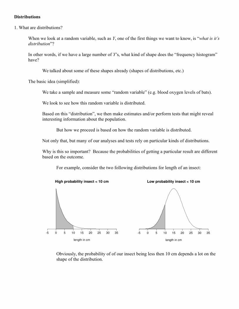
For example, consider the two following distributions for length of an insect:

Obviously, the probability of of our insect being less then 10 cm depends a lot on the shape of the distribution.

So here are some examples of examples of distributions:

If we toss a coin 25 times, and if Y = number of heads, then Y will have a binomial distribution

We write Y ~ Binomial.

The “~” symbol means “distributed as”

Often we put the parameters (more on this soon) of our distribution in parenthesis after the type of distribution, for example:

Y ~ Binom(25, 0.5)

Notice we abbreviated the distribution (we usually do).

What are 25 and 0.5? They are parameters (n = 25, and p = 0.5), but we'll save upthe details for another page or two.

If we measure heights of a sample of men on campus (Y = heights of men on campus), we can bepretty sure that Y will have a normal distribution.

We write Y ~ N

(The normal distribution is almost always abbreviated “N”).

2. The binomial distribution

We already used this distribution when we did probability.

Here it is again:

ny p y

1− pn− y

From now on we will definitely be using y in stead of j.

So what makes this a distribution?

Because we can use this to calculate all possible outcomes and then see what the distribution of Y looks like.

Here's an example using our coin. We toss it 10 times and note that n = 10, p = 0.5 (these are theparameters of our distribution, but more soon).

We get:

Heads Tails Probability

10 0 0.000989 1 0.009778 2 0.04395 (You should recognize7 3 0.11719 some of these numbers)6 4 0.205085 5 0.246094 6 0.205083 7 0.117192 8 0.043951 9 0.009770 10 0.00098Sum: 1.00000

A summary like this can be very useful. For example, we can now easily calculate the probability that Y = 0, 1 or 2 (where Y = number of heads):

Pr{0 ≤ Y ≤ 2} = 0.00098 + 0.00977 + 0.04395 = 0.05470

Also notice that if we add up all the possible outcomes we get 1.0:

Pr{0 ≤ Y ≤ 10} = 1.0

This is important but ought to be obvious: if we toss a coin, something has to happen, andthe above list is every single possibility!

If we want to see what the distribution of Y looks like we can plot it:

So what (finally), are parameters?

Parameters determine what our distribution looks like.

For a random variable, Y, we need to know two things to figure out what the distribution of Y looks like:

1) What kind of distribution Y has.

2) What the parameters of this distributions are.

Since we're looking at the binomial distribution, let's change the parameters and see what happens to Y:

Instead of n = 10 and p = 0.5, let's use n = 3 and p = 0.2.

Notice that now Y can go from 0 to 3.

So let's again calculate all the probabilities for Y:

Y Probability

0 0.512 1 0.384 2 0.096 3 0.008 Sum 1.000

And if we plot Y, this time our distribution looks rather different:

Again, to emphasize this: the parameters determine what our particular distribution looks like!

3. About distributions in general:

We've learned several things about distributions:

1) The shape of a distribution can vary based on the parameters.

2) All possible outcomes must add up to one.

a) If Y is discrete, this is easy. For example, with the binomial what we are saying is:

∑y=0

n

(ny ) py (1− p)n− y = 1

In other words, take take all possible values of y, put them into the binomial distribution formula, and add these up and you'll get 1.00.

b) If Y is continuous, then the area under the curve formed by our distributionwill add up to one.

How do we add up “all possible outcomes” if our distribution is continuous?

We need calculus.

Don't worry, you're not responsible for anything involving calculus.

But what we're saying is:

∫−∞

+∞

(continuous distribution of y) dy = 1

Historical note: the ∫ symbol is short for “sum” (same word in Latin). In calculus we can add up a sequence of infinitely small things, which, in this case must add up to one.

Let's use the normal distribution as an example.

4. The normal distribution

The importance of the normal distribution to statistics can not be overemphasized. The Germans even put this on the old 10DM bill!

Sometimes also known as the Gaussian distribution.

So what is it?

f ( y) =1

σ√2πe

−12

( y−μσ )

2

Good! Now you know everything, right? Seriously, here are a couple of examples:

We're looking at the height for adult men in the U.S. Somehow we know that:

μ = 69.5 inches, and σ = 2.9 inches

This gives us the following picture (note the scale on the x-axis):

Let's try plotting the number of eggs produced by the American Toad (Bufo americanus). Again, somehow we know that (numbers are very approximate this time):

μ = 10,000 eggs, and σ = 2,000 eggs

This time we get the following picture:

Which looks a lot like the last plot (are they actually the same?). Let's make some comments on the normal distribution. The curve peaks at the mean (μ). The inflection (direction of the curve) changes at ± σ.

In other words, the parameters for the normal distribution are μ and σ. If I know what these are, I know what my normal distribution looks like. Notice also that the normal distribution actually goes from - ∞ to + ∞.

Finally, we should mention that the area under the curve will add up to 1, or using calculus we can say (since this is calculus you are not responsible for this equation).:

∫−∞

+∞1

σ√2πe

−12

( y−μσ )

2

dy = 1

So now we know the normal distribution is and what it looks like. Why is it so important? For several reasons, but the two most important for us are the following:

1) Many things in biology, have a normal, or approximately normal distribution. For example, heights, weights, IQ, many blood hormone levels, etc.

2) Because of something called the Central Limit Theorem. Well get back to this, but for the moment you should realize that it implies that even if Y is not normally distributed, we can often still use a normal distribution in statistics to calculate probabilities. It is literally one of the most important theorems/results in statistics.

5. The normal distribution and probability:

Since many things in biology (and elsewhere) have a normal distribution, we need to learn how to answer probability questions using the normal distribution. For example, suppose Y = height of male basketball players, and we want to know:

Pr{Y < 6 } (Incidentally, notice that: Pr{Y < 6 } = Pr{Y ≤ 6 }. Why?)

What we're asking is, what's the probability a male basketball player is less than 6 feet tall? If you knowcalculus, then you might think we could do:

∫−∞

61

σ√2πe−

12

( y−μσ )

2

dy

Unfortunately we can't do the integration except for a few special values of y (notice also that we need toknow μ and σ). Instead, we wind up using normal distribution tables that list probabilities by approximating the above very precisely. In other words, if we want to figure out the probability that a male basketball player is less than 6 feet tall, we find a table with the appropriate values of μ and σ, and then find Pr{Y < 6 }.

The obvious problem is that we would need an infinite number of normal tables, one for every possible combination of μ and σ. This is obviously impossible, so we need to do something else.

What we do instead is use one normal distribution and then convert all our probability questions to use this distribution. The distribution that we will use is called the standard normal distribution. This distribution has μ = 0, and σ = 1 (= σ2). Here's a picture:

So how do we use this distribution? We need to convert the variable we're interested in (e.g.., basketballplayer height) into variable that has μ = 0 and σ = 1. To do this, we do the following:

1) Subtract the mean from the distribution we're looking at. This will obviously give you μ = 0.

2) Divide by the standard deviation of the distribution we're looking at. This will give you σ = 1.

We call this new number Z, for z-score, and we say Z ~ N(0,1)

Here’s the formula:

Z =Y−

So if we use Z instead of our original Y, we only need to list our areas in one table and then use the standard normal (or sometimes “z”) curve. Although we'll learn how to do this by hand, usually we let a computer (or fancy calculator) spit out the answer for us.

Let's do some examples to calculate some probabilities using the standard normal (or z) curve/tables:

Pr{Z > 1.78}: Let's look at what we want first (it's always a good idea to sketch/draw pictures ofwhat you want).

Our normal distribution table will give you the area less than a particular value of Z. So go into the table and find 1.73:

Read 1.5 off the column on the left side going down.

Read the “.03” off the top row going across.

Now read across and down until these two values (1.7 and .03 in our example) intersect, and write down that number.

This is the area of the normal curve that is below 1.73.

You should see 0.9582

So we can write Pr{Z < 1.73} = 0.9582

But we want the area above 1.73:

We remember that the total area under the curve = 1.0, so we can do:

1 - 0.9582 = 0.0418

And finally we can say:

Pr{Y > 1.73} = 0.0418

Comment: since the standard normal distribution is symmetrical around 0, you could alsodo the following:

Change the sign of the value we're interested in:

instead of 1.73, use -1.73.

Now we can just look up Pr{Y < -1.73} and we get 0.0418

This is a little bit of a shortcut - if it's confusing, don't worry about it and stick to previous method until you get comfortable with this.

Let's try Pr{-1.35 < Z < 0.62}:

Again, let's look at our area first:

Let's look up the values in the z-table for for 0.62 and -1.35:

Pr{Z < -1.35} = 0.0885

Pr{Z < 0.62} = 0.7324

And since we want the area between these two z-values, we can subtract one from the other:

Pr{-1.35 < Z < 0.62} = Pr{Z < 0.62} - Pr{Z < -1.35} = 0.6439

But of course, we usually deal with Y, not Z. So let's do a practical example. We'll figure out some probabilities for male African elephants (Loxodonta africana). Somehow we know the following:

μ = 7,400 kg and σ = 500 kg (the average is approximately correct, the standarddeviation is a guess)

a) Find the probability that a (random) elephant is 6,500 kg or less:

Pr{Y < 6,500}:

Convert to Z:

Z =6,500 − 7,400

500=−1.8

Note that Pr{Y < 6,400} ≡ Pr{Z < -1.8}

(The symbol “≡” means “exactly equivalent to”)

Before we go on, let's look at some pictures:

Notice that the areas are identical. Let's look up -1.8 in our table to get 0.0359

So Pr{Y < 6,400} = Pr{Z < -1.8} = 0.0359

b) Find the probability that an elephant is 8,000 kg or more:

Pr{Y > 8,000}:

Z =8,000 − 7,400

500= 1.2

Again, remember that Pr{Y > 8,000 = Pr{Z > 1.2}

Just one picture this time:

As usual, we want the area in gray. so we look up 1.2 in our table to get 0.8849. This time we need to subtract this result from 1:

Pr{Y > 8,000} = Pr{Z > 1.2} = 1 - 0.8849 = 0.1151

c) (Last one) find probability that an elephant is between 8,000 and 8,500 kg:

Pr{8,000 < Y < 8,500}:

This time we need two values of Z:

Z 1 =8,000 − 7,400

500= 1.2

Z2 =8,500 − 7,400

500= 2.2

We look up Z1 to get 0.8849

We look up Z2 to get 0.9861

So we have:

Pr{8,000 < Y < 8,500} = Pr{1.2 < Z < 2.2} = .9861 - .8849 = .1012

We're not done with distributions yet. We need to learn about what is called reverse lookup (howto use probabilities to look up Y values), and we also want to learn a bit about other distributions.