when is discretion superior to timeless perspective policymaking?

ARTICLE IN PRESS

Contents lists available at ScienceDirect

Journal of Monetary Economics

Journal of Monetary Economics 57 (2010) 266–277

0304-39

doi:10.1

$ I w

on Opti

Francisc

E-m1 Re

reached

optimal

journal homepage: www.elsevier.com/locate/jme

When is discretion superior to timeless perspective policymaking?$

Richard Dennis

Economic Research, Mail Stop 1130, Federal Reserve Bank of San Francisco, 101 Market St, CA 94105, USA

a r t i c l e i n f o

Article history:

Received 15 December 2008

Received in revised form

17 February 2010

Accepted 19 February 2010Available online 4 March 2010

JEL classification:

C61

E52

E58

Keywords:

Discretion

Timeless perspective

Policy evaluation

32/$ - see front matter & 2010 Elsevier B.V. A

016/j.jmoneco.2010.02.006

ould like to thank the editor, an anonymous r

mal Monetary Policy, 2008, for comments. Th

o or the Federal Reserve System.

ail address: [email protected]

lated to the timeless perspective, King and W

its stationary distribution under the optimal

commitment policy when analyzing transiti

a b s t r a c t

The monetary policy literature assumes increasingly that policy is formulated according

to the timeless perspective (Woodford, 1999a). However, by treating appropriately the

auxiliary state variables that characterize the timeless perspective equilibrium when

evaluating policy performance, this paper shows that discretionary policymaking can be

superior to timeless perspective policymaking and identifies model features that make

this outcome more likely. Using standard New Keynesian DSGE models, discretion is

found to dominate timeless perspective policymaking when the price/wage Phillips

curves are relatively flat, due, perhaps, to firm-specific capital (or labor) and/or Kimball

(1995) aggregation in combination with nominal rigidities. These results suggest that

studies applying the timeless perspective might also usefully compare its performance

to discretion, paying careful attention to how policy performance is evaluated.

& 2010 Elsevier B.V. All rights reserved.

1. Introduction

Much work in recent decades has been devoted to understanding how central banks should conduct monetary policy.It is now generally accepted that private sector expectations can be an important channel through which monetary policyoperates and that the time-consistency issues raised by Kydland and Prescott (1977) are a legitimate and materialpolicy concern. These concerns feature prominently in the monetary policy design literature, which emphasizes thedistinction between commitment and discretion and are taken seriously by central banks, many of whom have adoptedinflation targeting policy regimes. Although optimal commitment policies (Kydland and Prescott, 1980) have the obviousattraction of being optimal, they are unattractive in so much as their performance is attributable to a central bank thatexploits private-sector expectations in some arbitrary initial period while promising never to do so again. Becausediscretionary policies are known to be suboptimal and optimal commitment policies are not time-consistent and dependon arbitrary initial conditions, Woodford and coauthors have argued that monetary policy might better be conductedaccording to a ‘‘timeless perspective’’.

The timeless perspective approach to policy design was first outlined in Woodford (1999a), advanced as a solution tothe ‘‘initial period’’ problem that characterizes optimal commitment policies.1 At that time, Woodford (1999a) argued that

ll rights reserved.

eferee, Jinill Kim, Stephen Sauer, Andrea Tambalotti and participants at the Norges Bank Workshop

e views expressed in this paper do not necessarily reflect those of the Federal Reserve Bank of San

olman (1999) and Khan et al. (2003) analyze responses to exogenous shocks once the economy has

commitment policy. Unlike the timeless perspective, however, they do not propose to overwrite the

onal dynamics.

www.elsevier.com/locate/jme

dx.doi.org/10.1016/j.jmoneco.2010.02.006

mailto:[email protected]

ARTICLE IN PRESS

R. Dennis / Journal of Monetary Economics 57 (2010) 266–277 267

the initial period problem could be overcome if the central bank were to ‘‘adopt, not the pattern of behavior from now onthat would be optimal to choose, taking expectations as given, but rather the pattern of behavior to which it would have

wished to commit itself to at a date far in the past, contingent upon the random events that have occurred in the meantime.’’Simply put, the initial period problem ceases to be a problem once the initial period has long since passed. In subsequentwork, the concepts of timeless perspective policy making and timeless perspective equilibria have been refined and mademore formal.2 Because the timeless perspective overcomes the initial period problem, the literature on monetary policyhas embraced it, to the point where such policies increasingly form the backbone of policy analysis and one centralbank—Norges Bank—has employed the timeless perspective to construct its public interest rate forecasts.

Timeless perspective policies are closely related to optimal commitment policies. In particular, both policies involveauxiliary state variables that track the value of commitments over time. One implication of these auxiliary state variables isthat timeless perspective policies involve commitments and are not time-consistent in the sense of Kydland and Prescott(1977). At the same time, timeless perspective policies are not optimal in the sense of Kydland and Prescott (1980),opening the door to the possibility that they may be inferior to other suboptimal policies, such as discretion.

In this paper I ask whether discretionary monetary policy can dominate policy designed according to the timelessperspective and answer in the affirmative. The paper then examines the factors that govern this result, employing amicrofounded dynamic stochastic general equilibrium (DSGE) model to ascertain the role that nominal and real rigiditiesplay in determining whether discretion is superior. Indeed, it is shown that discretion is more likely to dominate timelessperspective policy making in models where nominal and real rigidities are important. Two additional contributions of thepaper are that it develops a measure of policy performance suitable for consistently evaluating timeless perspective anddiscretionary policies and that it shows how timeless perspective equilibria can be obtained from the solution to anunmodified formulation of the optimal commitment problem (cf. Woodford, 2003). It is important to compare theperformance of timeless perspective policies to discretion because such a comparison helps to identify and understandsituations where timeless perspective policy making may be inferior to discretion. More generally, such a comparisonallows us to better understand when discretionary policies perform well and when timeless perspective policies performless well.

Previous studies comparing discretion to timeless perspective policy making have tended to focus on unconditional losswhen evaluating policy performance3 (McCallum and Nelson, 2004; Sauer, 2007). However, there are several good reasonsnot to use unconditional loss for this purpose. One reason is that the loss function common to both the timeless perspectiveand discretionary optimization problems is (invariably) conditional. Another reason is that using unconditional loss toevaluate performance amounts to comparing discretion to the optimal commitment policy because the timelessperspective policy and the optimal commitment policy share the same asymptotic equilibrium. A third reason is that, byignoring transition dynamics, the use of unconditional loss can generate spurious performance reversals (Kim et al., 2008).Rather than use unconditional loss to compare the two policy strategies, in this paper a measure of conditional loss isdeveloped that is suitable for the task. Specifically, the paper shows how the auxiliary state variables that enter thetimeless perspective equilibrium can be ‘‘integrated out’’ to produce a measure of conditional loss that is invariant to themultiplicity that is known to characterize timeless perspective policy making (Woodford, 2003, Chapter 7), that remainsconditional on the natural state variables common to both decision problems and that does not ignore transition dynamics.For linear-quadratic models, this integration lowers the performance of the timeless perspective policy relative to theoptimal commitment policy by terms that quantify the conditional mean and the conditional volatility of the auxiliarystates.

Of course, it is far from automatic that the resulting measure of policy performance will permit a timeless perspective tobe dominated by discretion. However, using standard New Keynesian DSGE models, it is shown that factors that flatten theNew Keynesian Phillips curve, such as nominal price rigidity, firm-specific labor/capital and Kimball (1995) aggregation,can raise the conditional volatility (in particular) of the auxiliary state variables to the point where discretion becomes thesuperior policy. Indeed, the intuition for this result is reasonably clear. As the Phillips curve becomes increasingly flat, thecentral bank must generate greater volatility in real marginal costs in order to stabilize inflation. To the extent that realmarginal costs are correlated with the central bank’s other policy objectives, this volatility in real marginal costs raises thevolatility of the commitments that characterize the timeless perspective policy, penalizing its performance.

The remainder of this paper is organized as follows. Section 2 introduces the timeless perspective approach to policydesign and applies it to a simple New Keynesian model. Section 2 also shows why the treatment of the auxiliary states inthe loss function matters importantly for performance comparisons. Section 3 illustrates how standard control methods forrational expectations models can be used to construct and analyze the equilibrium of a timeless perspective policy.In addition, Section 3 shows how the auxiliary state variables can be conditionally integrated out to construct a measure ofpolicy performance that is easy to compute and that is suitable for comparing the performance of discretion and timelessperspective policies. Applying this measure of policy performance to the simple New Keynesian model introduced inSection 2 and Section 4 demonstrates that discretion can, indeed, be superior to timeless perspective policymaking.

2 See Woodford (2003), Giannoni and Woodford (2002a,b) and Benigno and Woodford (2003, 2006).3 Indeed, some have interpreted the term ‘‘timeless perspective’’ to mean that timeless perspective policies should be derived as the solution to an

unconditional optimization problem (Blake, 2001; Jensen and McCallum, 2002; Damjanovic et al., 2008). Since Woodford’s approach to timeless

perspective policy design does not do this, these studies have found that timeless perspective policies are not optimal from the timeless perspective.

ARTICLE IN PRESS

R. Dennis / Journal of Monetary Economics 57 (2010) 266–277268

Extending the analysis to a medium-scale DSGE model, Section 4 also shows that factors that flatten the slopes of the wageand price Phillips curves increase the likelihood that discretion will be superior to timeless perspective policymaking.Section 5 concludes.

2. Timeless perspective policymaking: design and performance

In this section a simple New Keynesian model is used to derive the optimal commitment policy as well as targetingrules for policy under the timeless perspective and discretion, respectively. With these policies in hand, the sectionconsiders two standard methods for assessing policy performance and shows that neither performance measure is entirelysatisfactory.

2.1. A simple example

Consider the following decision problem. The central bank seeks to choose the sequence of nominal interest rates fitg10

to minimize the loss function

L0 ¼ E0

X1t ¼ 0

btðp2

t þmy2t þni2t Þ; ð1Þ

where pt represents inflation, yt represents the output gap, b 2 ð0,1Þ denotes the subjective discount factor, m 2 ½0,1Þ andn 2 ½0,1Þ denote the weights on output and interest rate stabilization relative to inflation stabilization, respectively and E0

is the mathematical expectations operator conditional on period 0 information. Under certain circumstances, Eq. (1) can beviewed as a second-order accurate approximation to household welfare (Benigno and Woodford, 2006). For the purposes ofthis section, however, Eq. (1) is taken to be primal.

Constraining the central bank’s decision problem is the system

pt ¼ bEtptþ1þkytþut ; ð2Þ

yt ¼ Etytþ1�sðit�Etptþ1Þþrnt ; ð3Þ

utþ1 ¼ ruutþeutþ1; ð4Þ

rntþ1 ¼ rrrn

t þertþ1; ð5Þ

where ut represents a markup shock, rtn represents a neutral-rate shock and the initial conditions u0 and r0

n are known. Theinnovations eut and ert are assumed to be i.i.d. with zero mean and finite variance. Eq. (2) is the New Keynesian Phillipscurve obtained from a Calvo (1983)-pricing model. Eq. (3) is the standard consumption-Euler equation that, because themodel abstracts from government spending, investment and trade, is written in terms of the output gap. Eqs. (4) and (5)describe the laws of motion for the markup shock and the neutral-rate shock. The parameters fk,sg 2 ð0,1Þ denote theprice rigidity and the elasticity of intertemporal substitution, respectively, while fru,rrg 2 ð�1,1Þ summarize thepersistence properties of the two shocks.

2.2. Optimal commitment policy

The optimal commitment policy can be found by choosing fpt ,yt ,itg10 to minimize Eq. (1) subject to Eqs. (2)–(5). In

addition to (2)–(5), the first-order conditions for this decision problem are

bptþlptþ1 ¼ 0; t¼ 0; ð6Þ

mbyt�klptþ1þblytþ1 ¼ 0; t¼ 0; ð7Þ

bptþlptþ1�lpt�slyt ¼ 0; t40; ð8Þ

mbyt�klptþ1þblytþ1�lyt ¼ 0; t40; ð9Þ

nitþslytþ1 ¼ 0; tZ0; ð10Þ

where lptþ1 and lytþ1 are the Lagrange multipliers associated with Eqs. (2) and (3), respectively.The time inconsistency of the optimal commitment policy is reflected in the difference’s between Eqs. (6)–(7) and

(8)–(9), which imply a different policy when t¼ 0 than when t40. Notice, however, that these differences disappear whenlp0 ¼ ly0 ¼ 0. As a consequence, the optimal commitment policy can be obtained by applying standard saddle-pointsolution methods to Eqs. (2)–(5) and (8)–(10), with the initial conditions lp0 ¼ ly0 ¼ 0 and u0, r0

n, known.

ARTICLE IN PRESS


2.3. Timeless perspective policy

To obtain a Woodford (1999a) timeless perspective policy for this model we employ Eqs. (6)–(10) as follows. First, tointroduce the timeless perspective, assume that Eqs. (8) and (9) also apply when t=0, effectively discarding Eqs. (6) and (7).Then, to obtain a policy that is implementable, use Eq. (10) to solve for lytþ1 and Eq. (9) to solve for lptþ1 and substitutethese expressions into Eq. (8) to eliminate the two Lagrange multipliers. With these substitutions, the resulting timelessperspective policy is

ptþmk ðyt�yt�1Þ�

nskb ½ðbþskÞðit�it�1Þ�ðit�1�it�2Þ�þ

nb

it ¼ 0; tZ0: ð11Þ

Provided n40, Eq. (11) can be solved for it, giving rise to what is known as an explicit targeting rule. The timelessperspective equilibrium is now obtained by solving for the rational expectations equilibrium of Eqs. (2)–(5) and (11), withu0, i�1 and i�2 known. Notice that in this model the timeless perspective policy depends on the change in the output gap, apoint emphasized by Walsh (2003) in his discussion of ‘‘speed limit’’ policies and on lags of the interest rate, a pointWoodford (1999b) highlights in his analysis of optimal interest rate inertia. Further, reflecting the general property stressedby Giannoni and Woodford (2002b), because the shocks are not directly present, timeless perspective targeting rules, suchas Eq. (11), are robust to misspecification of the shock processes.

2.4. Discretion policy

The targeting rule characterizing discretion can be obtained in straightforward fashion using a variation on the methodintroduced by Cohen and Michel (1988). Because the only state variables in the model are the shocks, ut and rt

n, it must bethe case that Etptþ1 ¼ ypuruutþyprrrr

nt and Etytþ1 ¼ yyuruutþyyrrrr

nt , in any (Markov) time-consistent equilibrium, where

the coefficients ypu, ypr , yyu and yyr have yet to be determined. The discretionary control problem is then to choosefpt ,yt ,itg

10 to minimize the Lagrangean

L0 ¼ E0

X1t ¼ 0

bt½ðp2

t þmy2t þni2t Þþ2lptþ1ðpt�bðypuruutþyprrrr

nt Þ�kyt�utÞþ2lytðyt�ðyyuruutþyyrrrr

nt Þ

þsðit�ypuruutþyprrrrnt Þ�rn

t Þ�: ð12Þ

Differentiating Eq. (12) with respect to pt , yt and it produces the first-order conditions

ptþlptþ1 ¼ 0; tZ0; ð13Þ

myt�klptþ1þlytþ1 ¼ 0; tZ0; ð14Þ

nitþslytþ1 ¼ 0; tZ0; ð15Þ

which lead directly to the targeting rule

ptþmk yt�

nsk it ¼ 0; tZ0: ð16Þ

The (Markov) time-consistent equilibrium is then found by solving the rational expectations system described by Eqs.(2)–(5) and (16), yielding values for ypu, ypr , yyu and yyr .4

2.5. Policy performance

To compare the performance of the timeless perspective policy to those of the optimal commitment policy and thediscretion policy we need a method for evaluating the performance of the timeless perspective policy, an exercise that iscomplicated by the presence of the auxiliary state variables, yt�1, it�1 and it�2 in the timeless perspective targeting rule.Here, two standard methods for evaluating policy performance are considered.5 The first method is to evaluate lossconditional on the entire initial state vector, including the auxiliary states. The second method is to evaluate performanceusing unconditional loss. With the simple New Keynesian model serving to illustrate, it is shown that neither of thesemethods is entirely satisfactory.

Simplifying, in the special case that n¼ 0, Eqs. (11) and (16) collapse to

ptþmk ðyt�yt�1Þ ¼ 0; tZ0; ð17Þ

ptþmk

yt ¼ 0; tZ0; ð18Þ

4 Because this model does not contain any endogenous state variables, there is no need to iterate over ypu , ypr , yyu and yyr to obtain a fix-point.5 Sauer (2007) provides a related discussion.

ARTICLE IN PRESS

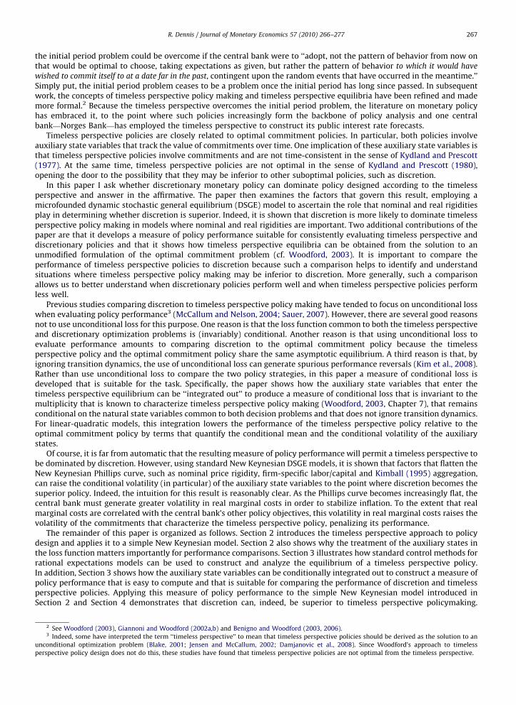
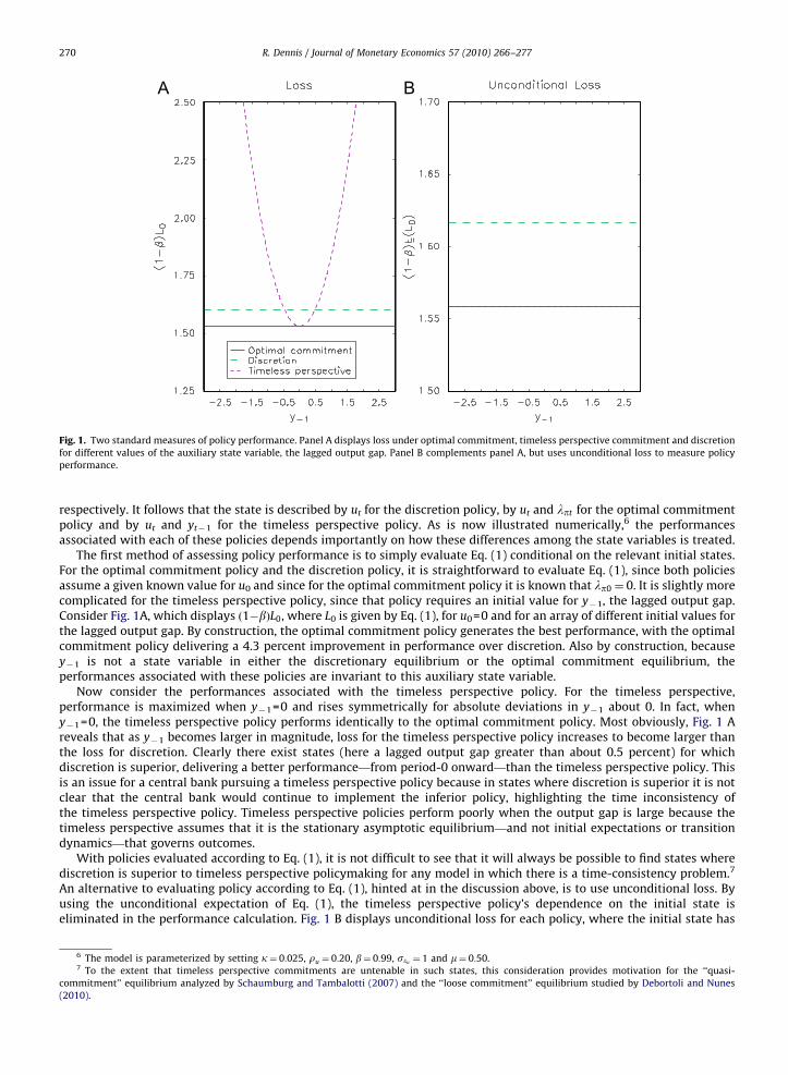
Fig. 1. Two standard measures of policy performance. Panel A displays loss under optimal commitment, timeless perspective commitment and discretion

for different values of the auxiliary state variable, the lagged output gap. Panel B complements panel A, but uses unconditional loss to measure policy

performance.


respectively. It follows that the state is described by ut for the discretion policy, by ut and lpt for the optimal commitmentpolicy and by ut and yt�1 for the timeless perspective policy. As is now illustrated numerically,6 the performancesassociated with each of these policies depends importantly on how these differences among the state variables is treated.

The first method of assessing policy performance is to simply evaluate Eq. (1) conditional on the relevant initial states.For the optimal commitment policy and the discretion policy, it is straightforward to evaluate Eq. (1), since both policiesassume a given known value for u0 and since for the optimal commitment policy it is known that lp0 ¼ 0. It is slightly morecomplicated for the timeless perspective policy, since that policy requires an initial value for y�1, the lagged output gap.Consider Fig. 1A, which displays ð1�bÞL0, where L0 is given by Eq. (1), for u0=0 and for an array of different initial values forthe lagged output gap. By construction, the optimal commitment policy generates the best performance, with the optimalcommitment policy delivering a 4.3 percent improvement in performance over discretion. Also by construction, becausey�1 is not a state variable in either the discretionary equilibrium or the optimal commitment equilibrium, theperformances associated with these policies are invariant to this auxiliary state variable.

Now consider the performances associated with the timeless perspective policy. For the timeless perspective,performance is maximized when y�1=0 and rises symmetrically for absolute deviations in y�1 about 0. In fact, wheny�1=0, the timeless perspective policy performs identically to the optimal commitment policy. Most obviously, Fig. 1 Areveals that as y�1 becomes larger in magnitude, loss for the timeless perspective policy increases to become larger thanthe loss for discretion. Clearly there exist states (here a lagged output gap greater than about 0.5 percent) for whichdiscretion is superior, delivering a better performance—from period-0 onward—than the timeless perspective policy. Thisis an issue for a central bank pursuing a timeless perspective policy because in states where discretion is superior it is notclear that the central bank would continue to implement the inferior policy, highlighting the time inconsistency ofthe timeless perspective policy. Timeless perspective policies perform poorly when the output gap is large because thetimeless perspective assumes that it is the stationary asymptotic equilibrium—and not initial expectations or transitiondynamics—that governs outcomes.

With policies evaluated according to Eq. (1), it is not difficult to see that it will always be possible to find states wherediscretion is superior to timeless perspective policymaking for any model in which there is a time-consistency problem.7

An alternative to evaluating policy according to Eq. (1), hinted at in the discussion above, is to use unconditional loss. Byusing the unconditional expectation of Eq. (1), the timeless perspective policy’s dependence on the initial state iseliminated in the performance calculation. Fig. 1 B displays unconditional loss for each policy, where the initial state has

6 The model is parameterized by setting k¼ 0:025, ru ¼ 0:20, b¼ 0:99, seu ¼ 1 and m¼ 0:50.7 To the extent that timeless perspective commitments are untenable in such states, this consideration provides motivation for the ‘‘quasi-

commitment’’ equilibrium analyzed by Schaumburg and Tambalotti (2007) and the ‘‘loose commitment’’ equilibrium studied by Debortoli and Nunes

(2010).

ARTICLE IN PRESS


been integrated out using the (unconditional) probability density implied by the model.8 Because policies are now beingevaluated according to the characteristics of their asymptotic equilibrium and the optimal commitment policy and thetimeless perspective policy share the same asymptotic equilibrium, these policies deliver the same unconditional loss.Clearly, if unconditional loss is used to measure performance, then discretion is the inferior policy.

However, although it is common to use unconditional loss when assessing timeless perspective policy performance,there are good reasons for not doing so. Aside from the most obvious point, which is that the discretionary problem, theoptimal commitment problem and the timeless perspective problem are all explicitly conditioned on an observed knowninitial state, it is well known that ignoring transition dynamics and evaluating policies according to their asymptoticbehavior can lead to spurious welfare reversals (Kim et al., 2008).

Fig. 1 A shows that discretion can be superior to timeless perspective policymaking, however neither Eq. (1) nor itsunconditional expectation are entirely satisfactory for quantifying timeless perspective policy performance: the formerdepends on auxiliary state variables, here y�1, while the latter ignores initial conditions and transition dynamics. Thefollowing section analyzes timeless perspective policymaking in the general linear-quadratic framework and develops ameasure of policy performance that is better suited to evaluating timeless perspective policies and to comparing theirperformance to discretion.

3. The general LQ framework

This section analyzes policy design in the general LQ framework and makes two main contributions. First, it presents asimple method for obtaining a timeless perspective equilibrium. Importantly, the solution method advanced belowrequires neither modifying the policy objective function nor introducing initial-period optimization constraints(cf. Giannoni and Woodford, 2002a, 2009, Woodford, 2003, Chapter 7; Benigno and Woodford, 2006). Instead, thesolution method engineers a timeless perspective equilibrium from the solution to the optimal commitment problem. Inaddition, the multiplicity known to characterize timeless perspective policymaking (Woodford, 1999a, 2003, Chapter 7) isdiscussed and illustrated.

Second, the section develops a metric to evaluate policy performance that is invariant to this multiplicity and that canbe applied consistently to timeless perspective policies and discretionary policies. To obtain this performance metric, theapproach is to integrate the conditional loss function with respect to the auxiliary state variables that are introduced bythe timeless perspective policy commitment. The result is a measure of policy performance that is invariant to themultiplicity that characterizes timeless perspective policymaking, that remains conditional on the natural state variablescommon to both discretion and the timeless perspective and that does not ignore transition dynamics.

3.1. The commitment solution

Let the economic environment be one in which an n�1 vector of endogenous variables, zt, consisting of n1

predetermined variables, xt and n2 (n2=n�n1) nonpredetermined variables, yt, evolves over time according to

xtþ1 ¼AxxxtþAxyytþBxuutþetþ1; ð19Þ

Etytþ1 ¼ AyxxtþAyyytþByuut ; ð20Þ

where ut is a p�1 vector of policy control variables, et � i:i:d:½0,R� is an s�1 ðsrn1Þ vector of white-noise innovations andEt is the private sector’s mathematical expectations operator conditional upon period t information. The matrices Axx, Axy,Ayx, Ayy, Bxu and Byu contain the structural parameters that govern preferences and technology and are conformable withxt, yt and ut as necessary. The matrix Ayy is assumed to have full rank.

Subject to Eqs. (19) and (20) and x0 known, the control problem is for the policymaker to choose the sequence of controlvariables futg

10 to minimize

E0

X1t ¼ 0

btðz0tWztþ2z0tUutþu0tRutÞ; ð21Þ

where zt � ½x0t y0t�0. Methods to solve this optimal commitment problem are by now well known (Oudiz and Sachs, 1985;

Backus and Driffill, 1986; Currie and Levine, 1993; Soderlind, 1999). For the purposes of this section, however, what isimportant is that the commitment equilibrium has the form

xtþ1 ¼MxxxtþMxpptþetþ1; ð22Þ

ptþ1 ¼MpxxtþMpppt ; ð23Þ

dt ¼ GdxxtþGdppt ; ð24Þ

8 Importantly, to the extent that observed data are not well explained by the model, very different results might be obtained if the integration used

the observed frequency distribution for the state variables rather than the model-implied density function.

ARTICLE IN PRESS


where dt �ytut

h iand pt is the n2�1 vector of shadow prices associated with the nonpredetermined variables and the system

is initialized with x0 known and p0=0. These shadow prices are the direct analog to the Lagrange multipliers employedearlier and they serve as state variables, keeping track of the current value of commitments, in the equilibrium (Kydlandand Prescott, 1980).

3.2. A timeless perspective solution

With the solution to the optimal commitment problem in hand, the next step is to use these equilibrium relationshipsto derive an expression for the shadow prices. Importantly, since dt contains all of the nonpredetermined variables and Ayy

has full rank, Gdp is an (n2+p)�n2 matrix with rank(Gdp)=n2. Rewriting Eq. (24) to make pt the subject leads to

pt ¼G�1dp ðdt�GdxxtÞ; ð25Þ

where Gdp�1 represents the generalized (left) inverse of Gdp. The last step is to substitute Eq. (25) into Eq. (22) and into the

lag of Eq. (23), thereby dispensing with the initial condition p0=0. After some reorganization, the timeless perspectiveequilibrium can be written as

xtþ1

xt

dt

264

375¼

Mxx MxpðMpx�MppG�1dp GdxÞ MxpMppG�1

dp

I 0 0

Gdx GdpðMpx�MppG�1dp GdxÞ GdpMppG�1

dp

2664

3775

xt

xt�1

dt�1

264

375þ

I

0

0

264

375½etþ1�: ð26Þ

To understand why this procedure recovers correctly a timeless perspective equilibrium, consider the relationshipbetween the optimal commitment problem and the timeless perspective problem. In both problems the policymaker hasaccess to a mechanism that allows it to commit to its policy. The value of the central bank’s policy commitments isencapsulated in shadow prices. Critically, aside from the initial period, the timeless perspective does not change either theconstraints or the objectives in the optimization problem. As a consequence, the timeless perspective does not change thesystem’s stability properties, nor does it change the system’s eigenvalues or whether the shadow prices are predetermined,which is why the optimal commitment policy and the timeless perspective policy share the same asymptotic equilibrium.What the timeless perspective does change, however, is the system’s initial conditions, which is why the optimalcommitment policy and the timeless perspective policy have different period-0 transition dynamics and, with discounting,yield different losses.

But, although saddle-point solution methods require the partitioning between stable and unstable eigenvalues toconform to the partitioning between predetermined and nonpredetermined variables (both unaffected by the timelessperspective), they do not require an explicit declaration of the initial conditions. As a consequence, the timeless perspectiveequilibrium can be found by first applying standard rational expectations control methods. Once the equilibrium has beenobtained for arbitrary initial conditions, the timeless perspective can be introduced by using the equilibrium relationshipsto solve for and subsequently eliminate the shadow prices.

3.2.1. Multiple representations of the timeless perspective solution

It is well-known that timeless perspective policies are not unique. To see the multiplicity, note the role of the rankcondition on Gdp. This rank condition ensures that the shadow prices obtained from Eq. (25) fully satisfy the model’sequilibrium relationships. It follows that a valid solution for pt can be obtained from any subset of the variables in yt and ut

provided that the resulting Gdp matrix has rank(Gdp)=n2. Although the particular state variables that enter the timelessperspective equilibrium will depend on which equilibrium relationships are used when solving for pt, by construction, theyall imply the same welfare and equilibrium behavior. The fact that timeless perspective equilibria have multiplerepresentations is also reflected in the fact that although the procedure described above yields an equilibrium in which ut

is a function of xt, xt�1, yt�1 and ut�1, the approach described in Section 2 would yield an equilibrium in which ut is afunction of xt, yt�1, ut�1 and ut�2.9

3.3. Evaluating policy performance

For the general linear-quadratic control problem described by Eqs. (19)–(21), the three policy approaches examinedabove have equilibria that can all be written in the form

stþ1 ¼MssstþNetþ1; ð27Þ

yt ¼Hysst ; ð28Þ

ut ¼ Fusst ; ð29Þ

9 Importantly, this well-known multiplicity of representations makes no material difference for the analysis or conclusions that follow, since it is

assumed—for consistency—that the conditioning variables satisfy the timeless perspective equilibrium relationships.

ARTICLE IN PRESS


where st � ½x0t q0t�0. For the discretionary policy qt is the null vector, for the optimal commitment policy qt=pt and for the

timeless perspective policy qt ¼ ½x0t�1 d0t�1�

0. Now, as Currie and Levine (1993) show in the continuous-time context, forarbitrary period t, Eqs. (27)–(29) allow the loss function, conditional on st, to be expressed as

Lt ¼ s0tPstþb

1�btrðN0PNRÞ; ð30Þ

where

P¼cWþbM0ssPMss; ð31Þ

cW �H0ysWHysþH0ysUFusþF0usU0HysþF0usRFus: ð32Þ

In light of Eq. (30), unconditional loss is given by

L ¼

Zs

s0tPstþb

1�btrðN0PNRÞ

� �pðstÞdst ¼ trðPXÞþ

b1�b

trðN0PNRÞ; ð33Þ

where p(st) denotes the density function for st and X represents the unconditional variance of st.The performances shown in Fig. 1 A were calculated using ð1�bÞLt , while those in Fig. 1 B were calculated using ð1�bÞL.

However, recognizing the deficiencies of these two performance measures, rather than assert initial values for the auxiliarystates, as Eq. (30) does and rather than integrate with respect to the entire state, st, as Eq. (33) does, I propose to integratewith respect to qt conditional on xt and to evaluate the performance of timeless perspective policies according to

bLt ¼

Zq

s0tPstþb

1�btrðN0PNRÞ

� �pðqtjxtÞ dqt ; ð34Þ

where pðqt jxtÞ denotes the density function for qt conditional on xt. To evaluate this integral, partition X (and subsequentlyMss and P) conformably with xt and qt, then the mean and variance of qt conditional on xt, are given by

qt ¼XqxX�1xx xt ; ð35Þ

Xqt jxt ¼Xqq�XqxX�1xx Xxq; ð36Þ

and Eq. (34) is equivalent to

bLt ¼ x0tðPxxþPxqXqxX�1xx þX�10

xx X0qxPqxÞxtþtrðPqqXqt jxt Þþb

1�btrðN0PNRÞ: ð37Þ

Eq. (37) contains three terms. The first and third terms represent the penalties attributable to the known initial stateand to the stochastic shocks, respectively. The second term represents the penalty associated with the conditional varianceof the auxiliary states that are introduced by timeless perspective policymaking. By integrating out the auxiliary statevariables, Eq. (37) measures average loss for a given state, xt. In the absence of any auxiliary states, Eq. (37) is equivalent toEq. (30). Further, in the limit as bm1, Eqs. (37) and (33), each scaled by ð1�bÞ, converge.

Before leaving this section, it is worth noting that policy performance, as assessed by Eq. (37), is invariant to how thetimeless perspective equilibrium is represented, unaffected by the particular choice of dt or by the fact that Gdp

�1 may not beunique. To understand why, note that the substantive difference between the optimal commitment equilibrium and thetimeless perspective equilibrium is that the shadow prices, pt, are not initialized to 0, but rather behave in the initial periodas they do in all subsequent periods. It follows that there is actually no need to eliminate the shadow prices from thesystem (the step that leads to multiple representations) when evaluating Eq. (37). Instead, one can simply integrate withrespect to the shadow prices conditional on xt. Because the optimal commitment policy has a unique representation interms of xt and pt (under standard and quite general conditions), so too does the timeless perspective equilibrium and thisunique representation yields unique values for the mean and variance of pt conditional on xt.

10

4. Two examples

In this section two New Keynesian models, each reflective of those employed in the monetary policy literature, areanalyzed to assess whether and when discretionary policy is superior to timeless perspective policy. For this exercise,policy performance is measured by Eq. (37). The first model is the simple New Keynesian model introduced for expositorypurposes in Section 2.1. The second model is a medium-scale DSGE model in the style of Christiano et al. (2005), Smets andWouters (2003) and Levin et al. (2006). The results from this second model are particularly interesting because it is highlyrepresentative of the workhorse models routinely used for monetary and much business cycle, analysis. In each model,policy performance is evaluated under discretion and the timeless perspective and, for a wide range of parameter values,the results indicate that discretion can be superior to the timeless perspective.

10 Without wishing to labor the point, this invariance property is also a feature of unconditional loss and for the same reason. Unconditional loss is

invariant to the multiplicity of representations because it integrates out the entire state vector, which includes the auxiliary states.

ARTICLE IN PRESS

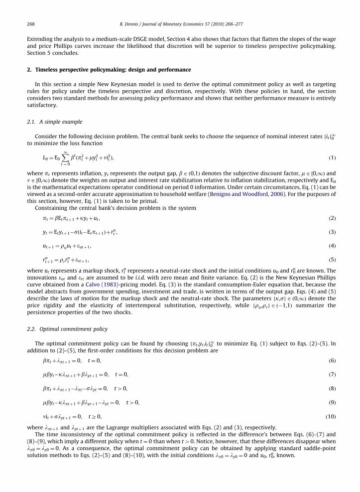
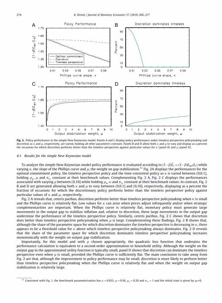
Fig. 2. Policy performance in the simple New Keynesian model. Panels A and C display policy performance under timeless perspective policymaking and

discretion as k and m, respectively, are varied, holding all other parameters constant. Panels B and D allow both k and m to vary and display as a percent

the occasions for which discretion performs better than the timeless perspective against particular values for k (panel B) and m (panel D).


4.1. Results for the simple New Keynesian model

To analyze the simple New Keynesian model policy performance is evaluated according to ð1�bÞbLt ¼ ð1�bÞEqjxðLtÞwhilevarying k, the slope of the Phillips curve and m, the weight on gap stabilization.11 Fig. 2A displays the performances for theoptimal commitment policy, the timeless perspective policy and the time-consistent policy as k is varied between (0,0.1],holding ru, m and seu constant at their benchmark values. Complementing Fig. 2 A, Fig. 2 C displays the performancesassociated with varying m between (0,10] while holding ru, k and seu constant at their benchmark values. In contrast, Fig. 2B and D are generated allowing both k and m to vary between (0,0.1] and (0,10], respectively, displaying as a percent thefraction of occasions for which the discretionary policy performs better than the timeless perspective policy againstparticular values of k and m, respectively.

Fig. 2 A reveals that, ceteris paribus, discretion performs better than timeless perspective policymaking when k is smalland the Phillips curve is relatively flat. Low values for k can arise when prices adjust infrequently and/or when strategiccomplementarities are important. When the Phillips curve is relatively flat, monetary policy must generate largemovements in the output gap to stabilize inflation and, relative to discretion, these large movements in the output gapundermine the performance of the timeless perspective policy. Similarly, ceteris paribus, Fig. 2 C shows that discretiondoes better than timeless perspective policymaking when m is large. Complementing these findings, Fig. 2 B shows that,although the share of the parameter space for which discretion dominates the timeless perspective is decreasing in k, thereappears to be a threshold value for k above which timeless perspective policymaking always dominates. Fig. 2 D revealsthat the share of the parameter space for which discretion dominates timeless perspective policymaking increasesmonotonically with the weight on output gap stabilization.

Importantly, for this model and with m chosen appropriately, the quadratic loss function that underpins theperformance calculation is equivalent to a second-order approximation to household utility. Although the weight on theoutput gap in the approximated utility function is typically small, panel D shows that discretion can dominate the timelessperspective even when m is small, provided the Phillips curve is sufficiently flat. The main conclusion to take away fromFig. 2 are that, although the improvement in policy performance may be small, discretion is more likely to perform betterthan timeless perspective policymaking when the Phillips curve is relatively flat and when the weight on output gapstabilization is relatively large.

11 Consistent with Fig. 1, the benchmark parameterization has k¼ 0:025, m¼ 0:50, ru ¼ 0:20 and seu ¼ 1 and the initial state is given by u0=0.

ARTICLE IN PRESS


4.2. Results for a medium-scale DSGE model

Having shown that discretion can be superior to the timeless perspective in the simple New Keynesian model, I nowundertake a broader analysis using a more sophisticated business cycle model that contains a wider array of shocks,rigidities and propagation mechanisms. Importantly, as with the simple model, the results indicate that discretion can besuperior to timeless perspective policymaking.

In this model, a unit-continuum of monopolistically competitive firms use capital and labor to produce according to aconstant-returns Cobb–Douglas production function. These firms set prices to maximize the expected discounted value ofthe firm, subject to a Calvo (1983) price rigidity and, following Smets and Wouters (2003), firms that cannot change theirprice in a given period are assumed to index their price to lagged aggregate inflation. The goods produced by these firmsare then aggregated according to a Kimball (1995) technology to produce an aggregate final good that is sold in a perfectlycompetitive market to households for consumption purposes and to firms for investment purposes. Investment goodspurchased by firms are combined with existing capital to produce new capital, as per Woodford (2005).

Households are monopolistic suppliers of their labor. They choose their consumption, nominal wage and holdings ofone-period nominal bonds to maximize their expected discounted lifetime utility. Following Erceg et al. (2000), householdsset their wage subject to a Calvo-style wage rigidity, with those households unable to change their wage assumed to indextheir wage to lagged aggregate inflation (Rabanal and Rubio-Ramırez, 2005). With respect to monetary policy, I assume, forsimplicity, that the central bank’s decision problem is to choose the interest rate on a one-period nominal bond to optimizethe expected discounted value of a quadratic loss function defined over inflation and the output gap, where the expectationis conditional on period-t information. A supplementary appendix that accompanies this paper provides the completelog-linear specification of the model.

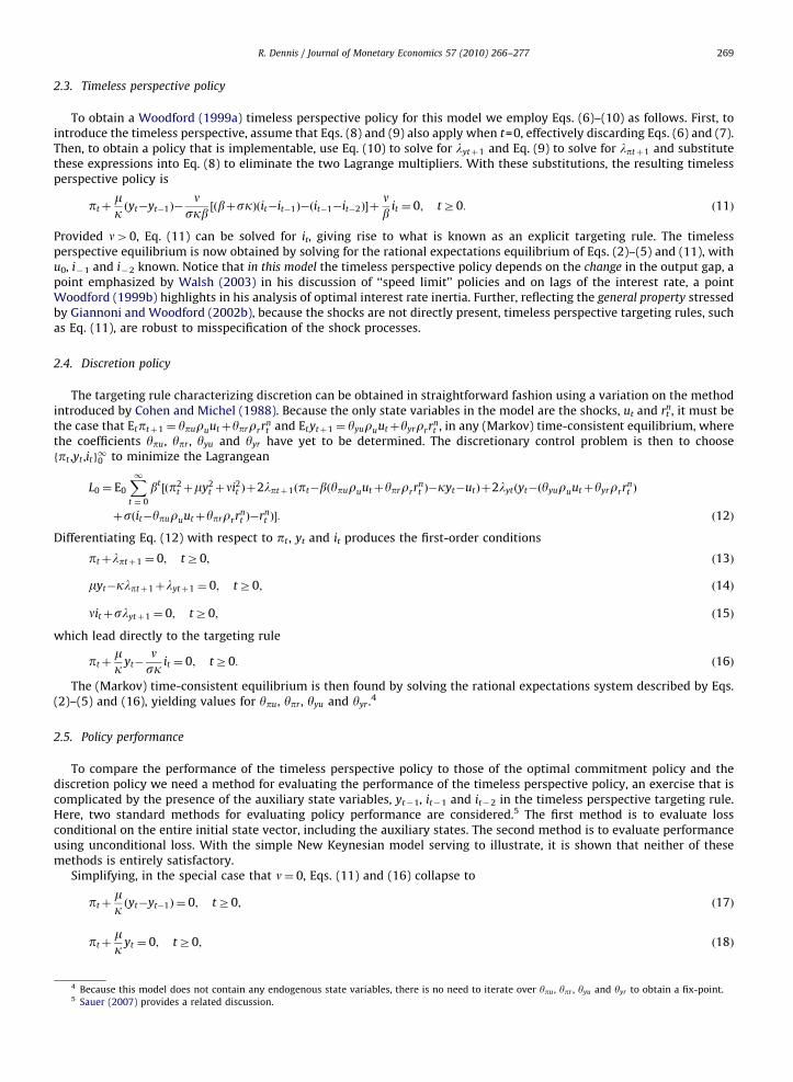
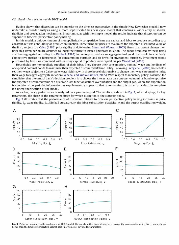
As earlier, policy performance is analyzed on a parameter grid. The results are shown in Fig. 3, which displays, for keyparameters, the share of the parameter space for which discretion is the superior policy.

Fig. 3 illustrates that the performance of discretion relative to timeless perspective policymaking increases as pricerigidity, xp, wage rigidity, xw, Kimball curvature, o, the labor substitution elasticity, f and the output stabilization weight,

Fig. 3. Policy performance in the medium-scale DSGE model. The panels in this figure display as a percent the occasions for which discretion performs

better than the timeless perspective against particular values of key model parameters.

ARTICLE IN PRESS


m, increase and declines as price indexation, ip, wage indexation, iw and the goods substitution elasticity, e, increase.12

Since higher values of xp imply a flatter price Phillips curve and higher values of xw imply a flatter wage Phillips curve, theresults in Fig. 3 A and C are consistent with those in Fig. 2 A. Similarly, higher values of o also serve to flatten the pricePhillips curve and higher values of f serve to flatten the wage Phillips curve, explaining why the relative performance ofdiscretion improves as these parameter increase (Fig. 3 E and G, respectively). With respect to m, the result in Fig. 3 H is alsoconsistent with the simple New Keynesian model. With respect to ip, iw and e, whether increases in these parameters helpor hinder discretion turns primarily on how they alter the trade-off the central bank faces between stabilizing inflation andstabilizing the output gap. With respect to e, higher values can help discretion because they lower the steady-stateconsumption share of output, weakening the policy channel operating on real marginal costs through consumption andwages. However, with the Kimball (1995) aggregator, higher values of e also steepen the slope of the price Phillips curve,which hinders discretion. In this model, on balance, the latter effect dominates. Higher values of ip and iw worsen therelative performance of discretion because these indexation parameters raise the importance of being able to manageprice-sector expectations in order to prevent adverse shocks from having enduring effects on price and wage inflation.

5. Conclusion

This paper has shown that discretion can be superior to timeless perspective policymaking and has identified factorsthat contribute to this outcome occurring. Broadly speaking, discretion is more likely to be superior to timeless perspectivepolicymaking when the Phillips curve is relatively flat, i.e., in models where nominal price rigidity is important and/orwhere factors such as Kimball aggregation or firm-specific labor/capital are present. These findings are important becausethese very factors are becoming widely employed in the New Keynesian DSGE models used to analyze monetary policy.Although a timeless perspective approach to policymaking has its attractions, one cannot simply assume that timelessperspective policymaking is superior to discretion.

One difficulty with comparing discretion to timeless perspective policymaking has been finding a suitable metric forassessing performance. This difficulty arises because the timeless perspective introduces auxiliary state variables that areabsent from the discretionary equilibrium. Rather than simply assigning initial values to these auxiliary state variables orusing unconditional loss to evaluate policies, this paper proposes to evaluate policies using a measure of conditional lossthat integrates out the auxiliary state variables conditional upon the known predetermined state variables. The resultingmeasure of policy performance is easy to compute, provides a consistent treatment of the initial conditions in thediscretion and the timeless perspective equilibria and is consistent with the conditioning assumptions that describe theassociated optimization problems.

The goal of this paper has not been to criticize the timeless perspective as an approach to policy design. Rather, becausetimeless perspective policies are suboptimal, the goal has been to highlight that timeless perspective policies are notnecessarily superior to other suboptimal policies, of which discretion is a leading example. Afterall, it is unclear why acentral bank should commit to implementing a timeless perspective policy when that policy is inferior to a time consistentalternative. The results in this paper suggest that studies analyzing timeless perspective policies might usefully considertheir performance alongside that of discretion, evaluating the policies using the measure of policy performance developedin this paper.

Appendix. Supplementary data

Supplementary data associated with this article can be found in the online version at doi:10.1016/j.jmoneco.2010.02.006.

References

Backus, D., Driffill, J., 1986. The consistency of optimal policy in stochastic rational expectations models. Centre for Economic Policy Research DiscussionPaper #124.

Benigno, P., Woodford, M., 2003. Optimal monetary and fiscal policy: a linear quadratic approach. In: Gertler, M., Rogoff, K. (Eds.), NBER MacroeconomicsAnnual 2003. MIT Press, Cambridge.

Benigno, P., Woodford, M., 2006. Linear-quadratic approximation of optimal policy problems. NBER Working Paper #12672 (version dated August 4,2008).

Blake, A., 2001. A timeless perspective’ on optimality in forward-looking rational expectations models. National Institute of Economic and Social ResearchWorking Paper #188 (version dated October 11, 2001).

12 In addition to these parameter, the model contains parameters for the depreciation rate on capital, d, the production coefficient on capital, a, the

Frisch labor supply elasticity, w, the elasticity of intertemporal substitution, s�1 and the capital adjustment cost, Z. However, to keep the exercise

manageable, d, a, w, Z and s and the parameters in the shock processes were held constant since preliminary investigations indicated these parameters

were largely unimportant for the results. Based on the estimates in Levin et al. (2006) and Smets and Wouters (2007), the model is parameterized by

setting b¼ 0:99, d¼ 0:025, a¼ 0:36, s¼ 2:19, w¼ 1:49 and Z¼ 5:74. In addition, the shock processes are parameterized according to rg ¼ rv ¼ 0:3 and

ru ¼ 0:95. Lastly, the initial state is parameterized on the assumption that the economy initially resides at its nonstochastic steady state.

10.1016/j.jmoneco.2010.02.006

10.1016/j.jmoneco.2010.02.006

ARTICLE IN PRESS


Calvo, G., 1983. Staggered contracts in a utility-maximising framework. Journal of Monetary Economics 12, 383–398.Christiano, L., Eichenbaum, M., Evans, C., 2005. Nominal rigidities and the dynamic effects of a shock to monetary policy. Journal of Political Economy 113,

1–45.Cohen, D., Michel, P., 1988. How should control theory be used to calculate a time-consistent government policy? Review of Economic Studies 55,

263–274Currie, D., Levine, P., 1993. Rules, Reputation and Macroeconomic Policy Coordination. Cambridge University Press, Cambridge.Damjanovic, T., Damjanovic, V., Nolan, C., 2008. Unconditionally optimal monetary policy. Journal of Monetary Economics 55, 491–500.Debortoli, D., Nunes, R., 2010. Fiscal policy under loose commitment. Journal of Economic Theory, in press.Erceg, C., Henderson, D., Levin, A., 2000. Optimal monetary policy with staggered wage and price contracts. Journal of Monetary Economics 46, 281–313.Giannoni, M., Woodford, M., 2002a. Optimal interest-rate rules: I. General theory. NBER Working Paper #9419 (version dated December 16, 2002).Giannoni, M., Woodford, M., 2002b. Optimal interest-rate rules: II. Applications. NBER Working Paper #9420 (version dated December 16, 2002).Giannoni, M., Woodford, M., 2009. Optimal target criteria for stabilization policy. Manuscript (version dated October 2, 2009).Jensen, C., McCallum, B., 2002. The non-optimality of proposed monetary policy rules under timeless perspective commitment. Economics Letters 77,

163–168.Khan, A., King, R., Wolman, A., 2003. Optimal monetary policy. Review of Economic Studies 70, 825–860.King, R., Wolman, A., 1999. What should the monetary authority do when prices are sticky? In: Taylor, J. (Ed.), Monetary Policy Rules. University of

Chicago Press, Chicago, pp. 349–396.Kim, J., Kim, S., Schaumburg, E., Sims, C., 2008. Calculating and using second order accurate solutions of discrete time dynamic equilibrium models.

Journal of Economic Dynamics and Control 32, 3397–3414.Kimball, M., 1995. The quantitative analytics of the basic neomonetarist model. Journal of Money, Credit and Banking 27, 1241–1277.Kydland, F., Prescott, E., 1977. Rules rather than discretion: the inconsistency of optimal plans. Journal of Political Economy 87, 473–492.Kydland, F., Prescott, E., 1980. Dynamic optimal taxation, rational expectations and optimal control. Journal of Economic Dynamics and Control 2, 79–91.Levin, A., Onatski, A., Williams, J., Williams, N., 2006. Monetary policy under uncertainty in micro-founded macroeconometric models. In: Gertler, M.,

Rogoff, K. (Eds.), NBER Macroeconomics Annual 2005. MIT Press, Cambridge, MA, pp. 229–287.McCallum, B., Nelson, E., 2004. Timeless perspective vs. discretionary monetary policy in forward-looking models. Federal Reserve Bank of St. Louis

Economic Review March/April, 43–56.Oudiz, G., Sachs, J., 1985. International policy coordination in dynamic macroeconomic models. In: Buiter, W., Marston, R. (Eds.), International Economic

Policy Coordination. Cambridge University Press, Cambridge, pp. 275–319.Rabanal, P., Rubio-Ramırez, J., 2005. Comparing New Keynesian models of the business cycle: a Bayesian approach. Journal of Monetary Economics 52,

1151–1166.Sauer, S., 2007. Discretion rather than rules? When is discretionary policy-making better than the timeless perspective? European Central Bank Working

Paper #717 (version dated January 23, 2007).Schaumburg, E., Tambalotti, A., 2007. An investigation of the gains from commitment in monetary policy. Journal of Monetary Economics 54, 302–324.Smets, F., Wouters, R., 2003. An estimated dynamic stochastic general equilibrium model of the euro area. Journal of the European Economic Association

1, 1123–1175.Smets, F., Wouters, R., 2007. Shocks and frictions in US business cycles: a Bayesian DSGE approach. American Economic Review 97, 586–606.Soderlind, P., 1999. Solution and estimation of RE macromodels with optimal policy. European Economic Review 43, 813–823.Walsh, C., 2003. Speed limit policies: the output gap and optimal monetary policies. American Economic Review 93, 265–278.Woodford, M., 1999a. Commentary: How should monetary policy be conducted in an Era of price stability? Federal Reserve Bank of Kansas City, New

Challenges for Monetary Policy, Kansas City.Woodford, M., 1999b. Optimal monetary policy inertia. The Manchester School Supplement 67 (supplement), 1–35.Woodford, M., 2003. Interest and Prices: Foundations of a Theory of Monetary Policy. Princeton University Press, Princeton, NJ.Woodford, M., 2005. Inflation and output dynamics with firm-specific investment. International Journal of Central Banking 1, 1–46.

when is discretion superior to timeless perspective policymaking?

Documents