what's right with macroeconomics? - free
TRANSCRIPT
What’s Right with Macroeconomics?
M3014 - SOLOW TEXT.indd i 21/11/2012 13:03
What’s Right with
Macroeconomics?
Edited by
Robert M. Solow
Institute Professor Emeritus, Massachusetts Institute of
Technology, USA, Co-founder and Chairman, Cournot
Foundation, Paris, France
Jean-Philippe Touff ut
Director, Cournot Centre, Paris, France
THE COURNOT CENTRE SERIES
Edward ElgarCheltenham, UK • Northampton, MA, USA
M3014 - SOLOW TEXT.indd iii 21/11/2012 13:03

© The Cournot Centre 2012
All rights reserved. No part of this publication may be reproduced, storedin a retrieval system or transmitted in any form or by any means, electronic, mechanical or photocopying, recording, or otherwise without the prior permission of the publisher.
Published byEdward Elgar Publishing LimitedThe Lypiatts15 Lansdown RoadCheltenhamGlos GL50 2JAUK
Edward Elgar Publishing, Inc.William Pratt House9 Dewey CourtNorthamptonMassachusetts 01060USA
A catalogue record for this bookis available from the British Library
Library of Congress Control Number: 2012941927
ISBN 978 1 78100 739 6 (cased)ISBN 978 1 78100 744 0 (paperback)
Typeset by Servis Filmsetting Ltd, Stockport, CheshirePrinted and bound by MPG Books Group, UK
M3014 - SOLOW TEXT.indd iv 21/11/2012 13:03
v
Contents
List of figures and tables vi
List of contributors viii
Preface xi
Acknowledgements xii
About the series: Professor Robert M. Solow xiii
Introduction: passing the smell test 1
Robert M. Solow and Jean- Philippe Touffut
1. The fireman and the architect 8
Xavier Timbeau
2. Model comparison and robustness: a proposal for policy
analysis after the financial crisis 33
Volker Wieland
3. The ‘hoc’ of international macroeconomics after the crisis 68
Giancarlo Corsetti
4. Try again, macroeconomists 90
Jean- Bernard Chatelain
5. Economic policies with endogenous innovation and Keynesian
demand management 110
Giovanni Dosi, Giorgio Fagiolo, Mauro Napoletano and Andrea
Roventini
6. Booms and busts: New Keynesian and behavioural
explanations 149
Paul De Grauwe
7. The economics of the laboratory mouse: where do we go from
here? 181
Xavier Ragot
8. Round table discussion: where is macro going? 195
Wendy Carlin, Robert J. Gordon and Robert M. Solow
Index 231
M3014 - SOLOW TEXT.indd v 21/11/2012 13:03

viii
Contributors
Wendy Carlin is Professor of Economics at University College London,
a Research Fellow of the Centre for Economic Policy Research (CEPR)
and a Fellow of the European Economics Association. She is a member of
the Expert Advisory Panel of the UK’s Office for Budget Responsibility
(OBR) and co- managing editor of Economics of Transition. Her research
focuses on macroeconomics, institutions and economic performance, and
the economics of transition.
Jean- Bernard Chatelain is Professor of Economics at the Sorbonne
Economic Centre (Université Paris 1 Pantheon Sorbonne) and Co-
director of the CNRS European Research Group on Money, Banking and
Finance. His research interests include growth, investment, banking and
finance, applied econometrics and statistical methodology.
Giancarlo Corsetti is Professor of Macroeconomics at Cambridge
University (previously at the European University Institute [EUI],
Rome, Bologna and Yale University). He is a consultant for the
European Central Bank, programme director at the Centre for Economic
Policy Research (CEPR), member of the European Economic Advisory
Group at the CESifo (Munich Society for the Promotion of Economic
Research) at the University of Munich, and co- editor of the Journal of
International Economics. His main fields of interest are international
economics, open- economy macroeconomics and the economics of cur-
rency areas.
Giovanni Dosi is Professor of Economics and Director of the Institute
of Economics at the Sant’Anna School of Advanced Studies in Pisa.
His major research areas include economics of innovation and tech-
nological change, industrial organization and industrial dynamics,
theory of the firm and corporate governance, economic growth and
development.
Giorgio Fagiolo is Associate Professor of Economics at the Sant’Anna
School of Advanced Studies, Pisa, and holds a tenured position at
the Institute of Economics and the Laboratory of Economics and
Management. His research interests include agent- based computational
M3014 - SOLOW TEXT.indd viii 21/11/2012 13:03
Contributors ix
economics, complex networks, evolutionary games, industrial dynamics,
and economic methodology.
Robert J. Gordon is Stanley G. Harris Professor in the Social Sciences at
Northwestern University, a Research Associate of the National Bureau
of Economic Research (NBER), a Research Fellow of the Centre for
Economic Policy Research (CEPR) and of the OFCE (French Economic
Observatory, Sciences Po) in Paris. His research interests span macroeco-
nomic studies of inflation, unemployment, and both short- run and long-
run productivity growth as well as microeconomic work on price index
bias and the value of new products.
Paul De Grauwe is Professor of European Political Economy at the
London School of Economics. He is director of the Money, Macro and
International Finance Research Network of the CESifo (Munich Society
for the Promotion of Economic Research) at the University of Munich,
and a research fellow at the Centre for European Policy Studies in
Brussels. He was a member of the Belgian parliament from 1991 to 2003.
His research interests are international monetary relations, monetary inte-
gration, theory and empirical analysis of foreign- exchange markets, and
open- economy macroeconomics.
Mauro Napoletano is Senior Economist at the OFCE (French Economic
Observatory, Sciences Po) in Paris and Sophia- Antipolis, France. He
is an affiliated research fellow of the Laboratory of Economics and
Management (LEM) in Pisa and of the SKEMA Business School in
Sophia Antipolis. His research interests include the study of economic
models with heterogeneous agents in macroeconomics, the empirical
analysis of economic time series, and industrial dynamics.
Xavier Ragot is a Researcher at the CNRS (the French National Center
for Scientific Research) and an Associate Professor at the Paris School of
Economics. He was senior economist at the Bank of France from 2008
to 2011. He also served as chief economist of the French Agency for
Industrial Innovation. His main field of interest is monetary economics
and fiscal policy. His research focuses on liquidity issues, using the tools of
incomplete market theory and the computation of equilibria.
Andrea Roventini is Assistant Professor of Economics at the University
of Verona, Italy. He is an affiliated research fellow of the Laboratory
of Economics and Management (LEM) at the Sant’ Anna School of
Advanced Studies in Pisa, Italy, and of the OFCE (French Economic
Observatory, Sciences Po) in Paris and Sophia- Antipolis. His major
research areas include agent- based computational economics, business
M3014 - SOLOW TEXT.indd ix 21/11/2012 13:03

x What’s right with macroeconomics?
cycles, applied macroeconometrics, and the statistical properties of micro-
economic and macroeconomic dynamics.
Robert M. Solow is Institute Professor Emeritus of Economics at the
Massachusetts Institute of Technology. He received the Bank of Sweden
Prize in Economic Sciences in Memory of Alfred Nobel in 1987 for
his contributions to economic growth theory. He is Robert K. Merton
Scholar at the Russell Sage Foundation, where he is a member of the advi-
sory committee for the Foundation’s project on the incidence and quality
of low- wage employment in Europe and the USA. Co- founder of the
Cournot Centre, he is also co- founder of the Cournot Foundation.
Xavier Timbeau is Director of the Forecast and Analysis Department
of the OFCE (French Economic Observatory, Sciences Po). He teaches
macroeconomics and environmental economics at Supélec and Sciences
Po, Paris. His main research interests include unemployment and infla-
tion estimations, the economic outlook for the eurozone, the real- estate
market, as well as public accounts and intangible assets.
Jean- Philippe Touffut is Co- founder and Director of the Cournot Centre.
His research interests include probabilistic epistemology and the explora-
tion of evolutionary games from neurological and economic perspectives.
Volker Wieland is Professor of Monetary Theory and Policy in the House
of Finance at Goethe University of Frankfurt and a Founding Professor
of the Institute for Monetary and Financial Stability. He is also a research
fellow of the Center for Economic Policy Research in London, a member
of the CEPR’s Euro Area Business Cycle Dating Committee, advisory
editor of the Journal of Economic Dynamics and Control and programme
director for Central Banking and Monetary Economics at the Center for
Financial Studies in Frankfurt.
M3014 - SOLOW TEXT.indd x 21/11/2012 13:03
1
Introduction: passing the smell test
Robert M. Solow and Jean- Philippe Touffut
What is the relevance of macroeconomics today? The crisis that has been
raging since 2007 has spread to economic theories, and it might seem that
it is no longer possible to do macroeconomics as before. But what version
of macroeconomics was at fault here? Macroeconomic questions have
not really changed: they examine growth and fluctuations of the broad
national aggregates (national income, employment, inflation, investment,
consumer spending or international trade). How are these fundamental
aggregates determined, and how differently should we think about them?
The economic world is too complex to be thought about ‘raw’, so the use
of a model to answer these questions helps make deductions and justify
conclusions. It is easier, then, to perceive what beliefs they have been based
on, and to challenge them. Economic concepts are not built to be put on a
computer and run.1 It is thus all the more important to point out fragility
or recklessness wherever it appears. If intuition does not suffice to reject
the hypothesis and reasoning, then experimentation must confirm our
instincts: does it pass the smell test?
Economists do not directly perceive the concreteness of their w orld, but
engage in diverse manoeuvres that seek to prepare that world for investi-
gation. Using various abstractions and omissions, they build models to
describe simple imaginary stage sets. Models are constructed rather than
discovered; they are socially built because scientific work is an intrinsically
social activity. If economic models of human interactions are socially con-
structed by economists, the social world is not constructed by the model-
ling practices of economists. It is from this standpoint that the authors of
this volume offer to take stock of their discipline, with all its variety, from
ancient to modern macro, or vice versa.
Since the late 1970s, a majority of macroeconomists have focused
on developing what they call the ‘modern macroeconomics of business
cycle fluctuations’. Until the world entered a crisis initiated by subprime
mortgage defaults, excessive leveraging followed by deleveraging, output
and employment meltdowns and destruction of perceived wealth, there
was a common belief that macroeconomic truth had been discovered. A
M3014 - SOLOW TEXT.indd 1 21/11/2012 13:03

2 What’s right with macroeconomics?
consensus had emerged about models that combined new- classical market
clearing with the New- Keynesian contribution of sticky prices and other
frictions. Along the way, contributions to this current had concluded that
the great moderation of macroeconomic volatility in the 1984–2007 period
was a positive side effect of their analysis. Neither the proponents of
‘modern macro’ nor the adherents of Keynesian ideas anticipated the crisis
in advance (although there were exceptions, and mostly on the Keynesian
side).
This book is consequently neither a programme of intellectual conserva-
tism nor a nostalgic manifesto. Its discussion of the past, current or future
state of macroeconomics is not a matter of being for or against a model.
It does not argue that sounder economic reasoning will imply abandon-
ing the use of formal mathematical analysis. Models provide a formal
summary of how one experiences the economy: there is a set of variables,
and the logical relationships between them represent economic processes.
They make it easier to see how strong the assumptions must be for an
argument to be valid, and how different conclusions depend on slight
deviations in specific assumptions. How well they do that depends on how
closely the assumptions resemble the world we live in. Economics is not
the physics of society, and policy advisers cannot apply economics the way
engineers use physical models.2 History has shown that economic analysis
should result in a collection of models contingent on circumstances, and
not in a single, monolithic model for all seasons.
Our focus here is the relevance of contemporary macroeconomic
ideas, which implies going back to the hypotheses and the causalities that
founded the discipline. Fundamental macro still appeals to economists in
its early versions. If you wake any economist in the middle of the night,
our bet is that he or she would automatically think according to early
macro, whether you choose to call it ‘1978- era macro’ as Robert Gordon,3
‘primeval macro’ as Paul Krugman,4 or ‘eclectic Keynesianism’ as Robert
Solow. Old- fashioned macro remains a useful tool for carrying out practi-
cal policy analysis. At times like the present, when the (world) economy is
clearly suffering from almost universal shortage of demand, policy analy-
sis has little need of ‘micro- founded’ intertemporal maximization. The
quasi- static goods–bonds–money model respects the essential added- up
constraints and represents the motives and behaviour of individuals in a
sensible way, without containing any superfluous moving parts.5
Old- fashioned macro can even help us think about the relationships
between markets and how the whole system fits together, not only produc-
ing two goods, but multiple goods where some pairs of goods might be
substitutes or complements. Three decades of rational expectations, equi-
librium business cycles, the new economy, or rescue plans have nonetheless
M3014 - SOLOW TEXT.indd 2 21/11/2012 13:03
Introduction: passing the smell test 3
shown that debates about the actual state of affairs are always informed,
sometimes implicitly, by old- fashioned macro. Although the traditional
framework has remained the basis for most discussion, it has increasingly
been pushed out of universities and research centres. As expressed in jour-
nals, conferences and speeches, ‘modern macro’ has become dominant.
Throughout the book, the contributors recurrently wonder in what
ways this modern version belongs in ‘macro’. Focus on individual prefer-
ences and production functions misses the essence of macro fluctuations,
the coordination failures and the macro externalities that convert interac-
tions among individual choices into constraints that prevent workers from
optimizing working hours and firms from optimizing utilization, produc-
tion and sales. By definition, modern macroeconomic models exclude
involuntary unemployment (except through wage rigidities) and possess
perfect capital markets; they fail to reproduce the observed dynamics of
the economy with reasonable parameters. They had nothing useful to
say about anti- recession policy, because they had built into implausible
assumptions the impossibility of a crisis. They concluded that there was
nothing for macroeconomic policy to do.
On the policy front, the precision of the model created the illusion that a
minor adjustment in the standard policy framework could prevent future
crises. With the economy attached to a highly leveraged, weakly regulated
financial system, such reasoning and consequential inaction have proved
unfounded. And the approach was no less false in earlier recessions that
followed different patterns. If many economists have been led astray by
reliance on certain categories of formal models, the consequences of such
oversights have not only been methodological, but have challenged the
legitimacy of the profession. This book wants to help expand the conver-
sation on realism in macroeconomics. The contributors do not want the
same answer for everything; they are looking for as many answers as there
are questions.
In Chapter 1, Xavier Timbeau describes the contemporary challenge
of economics by putting into perspective the criticisms of modern macro-
economics. Why do so many publications have so little to say about the
crisis? Is this a failure of modern economic research in general, or specifi-
cally that of the dominant theory? The crisis has represented a profound
violation of its world view, and has challenged many of its axioms. How
can one determine a permanent income in such an event? How can one
imagine companies going through the crisis independently of their balance
sheet structure? How can one believe that people have reliable knowledge
about the future when governments are embarking on massive stimulus
packages? It becomes impossible to defend unrealistic axioms in the face
of such overwhelming questions. The crisis has shown that uncertainty
M3014 - SOLOW TEXT.indd 3 21/11/2012 13:03

4 What’s right with macroeconomics?
is radical, and the heterogeneity of agents is central to human activity.
These two elements interact, and one cannot analyse the economy without
taking into consideration the nature of expectations. The crisis invites
us to re- evaluate experimentation: it does not involve choosing the most
realistic model out of a set of models, knowing that even the most realistic
one is not credible.
A systematic comparative approach to macroeconomic modelling is
proposed by Volker Wieland in Chapter 2, with the objective of identify-
ing policy recommendations that are robust to uncertainty. By examin-
ing multiple structural macroeconomic models, he evaluates their likely
impact if applied. Wieland suggests organizing a level playing field on
which models can compete and empirical benchmarks – which the models
must satisfy to stay in the race – can be determined. The breadth of the
models covered makes it possible to compare vintage and more recent
Keynesian- style models for a given country or cross- country comparison
between the United States, the euro area and some small open economies.
Whatever the case, the assessment concerns standard New- Keynesian
dynamic stochastic general equilibrium (DSGE) models and DSGE
models that also include some financial or informational frictions. In the
latter case, the agents are so clever that they even know the model in which
they are being studied. The result is that the models’ forecasts perform
differently from one period to another. In recession times, no single model
dominates the others. By construction, models are in fact incapable of
forecasting crises. This was not only true for the 2008–09 period, but also
for the four preceding ones. Even a thorough construction of the financial
sector, with the inclusion of learning and beliefs, can only make a crisis
conceivable, and possibly understandable.
From the perspective of an international economist, in Chapter 3,
Giancarlo Corsetti carries out an admittedly biased review of emerging
issues in macroeconomics. This involves judging the vitality of different
macroeconomic currents based on questions that the crisis is forcing us to
address. How are shocks transmitted? What is the role of financial chan-
nels in magnifying shocks or in translating financial disturbances into
real ones? What is the extent of misallocation at the source? Corsetti con-
centrates on the opposition between liquidity runs versus policy/market
distortions. Both must be overcome theoretically as much as politically: it
is a question of guarantees versus market discipline, implying the removal
or correction of policy. A highly stylized model discusses over- borrowing
and exchange rate misalignments as general features of economies in
which financial markets are incomplete. How can one build the frame-
work in which the international dimensions of the crisis, ranging from
global imbalances, to fiscal crisis and cross- border contagion, have so far
M3014 - SOLOW TEXT.indd 4 21/11/2012 13:03
Introduction: passing the smell test 5
typically been analysed as independent phenomena rather than as parts of
the same process?
In Chapter 4, Jean- Bernard Chatelain lays out the historical condi-
tions of how models are adopted and re- evaluated. Research results shape
people’s beliefs, and policy advice based on economic theories shapes
economic policies. These in turn shape the economy. People’s beliefs and
economic facts are connected through mechanisms of self- fulfilment and
self- defeat. In ‘modern macro’, models give a complete description of a
hypothetical world, and its actors are assumed to understand the world
in the same way it is represented in the model. When the complete eco-
nomic systems happen to resemble experience, they are so pared down
that everything about them is either known, or can be made up. Although
fundamental to contemporary macroeconomics, questions such as (a) the
impact of banking leverage, (b) interbank liquidity, (c) large shocks, (d)
fire sales and (e) systemic crisis have consequently remained dangerously
unaddressed. If weakly regulated financial sectors can be integrated into
the models and the efficient capital market hypothesis can be rejected,
then economists must investigate beyond macroeconomic policies. They
will have to examine the interplay between innovative macroeconomic
strategies and feasible banking and financial regulatory policy at the micro
level, as well as political economy issues.
If the crisis has set a major challenge for alternative theories, those which
link micro- behaviour with aggregate dynamics have a major advantage. In
Chapter 5, Giovanni Dosi and his colleagues develop an evolutionary
model, which goes back to basic Keynesian issues. The model first exam-
ines the processes by which technological change affects macro variables,
such as unemployment, output fluctuations and average growth rates.
The model then deals with the way endogenous, firm- specific changes in
the supply side of the economy interact with demand conditions. Finally,
the chapter explores the possible existence of long- term effects of demand
variations. Is long- term growth only driven by changes in technology, or
does aggregate demand affect future dynamics? Are there multiple growth
paths whose selection depends on demand and institutional conditions?
In Chapter 6, Paul De Grauwe tackles the subject of strong growth
followed by sharp declines. His model, written in the behavioural vein, is
compared to a DSGE model where agents experience no cognitive limita-
tions. De Grauwe’s hypothesis forces agents to use simple rules to forecast
output and inflation, and rationality is introduced by assuming a learning
mechanism that allows for the selection of those rules. What information
is available to the agents? When and how do they correct their beliefs?
Are their expectations the same during periods of growth and periods of
crises? In the DSGE model, large booms and busts can only be explained
M3014 - SOLOW TEXT.indd 5 21/11/2012 13:03
6 What’s right with macroeconomics?
by large exogenous shocks. Price and wage rigidities then lead to wavelike
movements of output and inflation. Thus, booms and busts are explained
exogenously. Although it does not introduce financial markets and the
banking sector, the behavioural model provides an endogenous explana-
tion of business cycle movements. The inflation targeting regime turns out
to be of great importance for stabilizing the economy in both models. In
the behavioural model, this follows from the fact that credible inflation
targeting also helps to reduce correlations in beliefs and the ensuing self-
fulfilling waves of optimism and pessimism. Its conclusion is meaningful:
strict inflation targeting cannot be an optimal policy.
Among the numerous rival research programmes, what were the crite-
ria, and which programmes were adopted? In Chapter 7, Xavier Ragot
provides an original perspective by placing himself in the position of the
laboratory mouse, whose trajectory itself is the subject of observation.
Within this framework, he endeavours to formalize Keynesian intui-
tions. The benchmarks of economic research have themselves been under
debate: should they be able to reproduce past historical data, make better
predictions than the others, or make fewer mistakes, and over what time
horizon? A considerable simplification in the modelling strategy has
clearly been decisive. In the dominant current, it has reduced macroeco-
nomics to microeconomics, with one sole agent and one good. Ragot eval-
uates how the questions of information and frictions on the markets have
challenged or reinforced the programme. New questions, however, are still
being posed inside the community of economists. Like lab mice, research-
ers look for the cheese without knowing which labyrinth they were put in,
and they may find themselves at a loss if the cheese is suddenly moved. The
effervescence in the work produced by economists has not been on a par
with the issues at stake. A new research programme and perhaps a new
paradigm are needed, Ragot believes, and the cheese may have to wait a
long time if the mice are in the wrong maze.
In the round table discussion that concludes this volume (Chapter 8),
Wendy Carlin recalls the experience of the euro. The eurozone’s first
decade was celebrated as a success, before it was swiftly followed by a
major crisis. Beneath the surface of the successful achievement of inflation
close to target and a modest output gap for the eurozone as a whole, the
diverse performance of its members reflected the failure of countries to
implement stabilization policy at the national level in response to country-
specific shocks. The macroeconomic apparatus at stake in Europe was not
simply a powerful modelling tool, and its methods and recommendations
may not have been at the service of building and improving the policy
regime. It has rather dictated or defined those things. Fundamentally,
good models of the leverage cycle need to be built to incorporate distribu-
M3014 - SOLOW TEXT.indd 6 21/11/2012 13:03
Introduction: passing the smell test 7
tional effects. If a process is underway of moving to a new macroeconomic
paradigm and policy regime, in what ways will it contain the seeds of the
next crisis?
Robert J. Gordon takes an American perspective to clarify the co-
existence of the Great Depression, the Japanese lost decade(s) and the
Great Moderation followed by the Great American Slump. From the
structure of shocks and propagation mechanisms, what can be learned
from history about shocks? What are the propagation mechanisms that
are essential to explaining this history? To answer these questions, Gordon
points out, just as the other contributors to this book, that economists
must not be too parsimonious: their ‘models must be as simple as possible,
but not more so’.6
NOTES
1. Lucas, R. (1988), ‘On the mechanics of economic development’, Journal of Monetary
Economics, 22(1), July, 3–42.
2. Among the pioneers who developed mathematical modelling for the social sphere,
Augustin Cournot (1801–77) affirmed the mathematization of social phenomena as an
essential principle. He made clear, however, that economics could not be constructed as
an axiomatically based hard science, and that the scientific approach for understanding
how society functions should not lead, in and of itself, to policy recommendations.
3. Gordon, R.J. (2009), Is Modern Macro or 1978- era Macro more Relevant to Understanding
the Crisis?, Contribution to the International Colloquium on the History of Economic
Thought, Sao Paulo, Brazil, 3 August.
4. Krugman, P. (2012), ‘There is something about macro’, MIT course, available at: http://
web.mit.edu/krugman/www/islm.html.
5. Krugman, P. (2012), ‘The macro wars are not over’, The New York Times, 23 March.
6. Quote from Albert Einstein by Robert Solow during the round table.
M3014 - SOLOW TEXT.indd 7 21/11/2012 13:03

8
1. The fireman and the architect
Xavier Timbeau1
INTRODUCTION
The disaster film The Towering Inferno (1974) is set in a newly constructed
tower. The architect, played by Paul Newman, has devised a sophisticated
security system that makes this tower perfectly safe, despite its great height
and elegant design. Through greed, however, the building contractors
and the architect’s associates have not followed the requirements and
recommendations of the architect. Since the technical specifications have
not been respected, the tower is going to become a death trap. Boldness
becomes arrogance, and the folly of man leads to a tragic fate. When the
fire breaks out, the first reaction is to blame the security system for being
defective. The design of the tower is so remarkable, however, that a fire is
quite simply impossible, and the monitoring system is really only there to
reassure the sceptics. A second character then comes on the scene. This is
the fire chief, played by Steve McQueen. For him, no design is infallible,
however advanced it may be. Each fire is unique, and must be fought, at
the risk of his life, in this case because 150 people are trapped at the top of
the tower and need to be saved.
We can use this story as a metaphor for the crisis we are currently in.
The architects designed a new world, which they believed to be infallible.
All previous achievements paled into insignificance beside the audacity
of this architecture. But then, either because certain people, motivated by
their own self- interest and cupidity, perverted the initial plan to such an
extent that they turned it into a death trap, or because it is naive to believe
that any design can be infallible, the defects, as always, came out in the
end: the catastrophe occurred. And then the fire fighters were called out to
try to remedy the situation, or at least to limit the damage.
Since it started in August 2007, the economic crisis has wrought havoc
in our world. The repercussions are still being felt. And for those endeav-
ouring to think about and understand how economies work, it represents
an inescapable challenge. It is not possible to carry on doing macroeco-
nomics as before. Like the Great Depression of the 1930s, the ‘Great
M3014 - SOLOW TEXT.indd 8 21/11/2012 13:03
The fireman and the architect 9
Recession’, as it is now called, has sent shock waves through the hushed
circles of economists.
That is all the more so, since, just before the crisis, contemporary mac-
roeconomics had reached a new consensus. A new synthesis, between
the New Classicists and the New Keynesians, had produced a dominant
corpus, driving alternative approaches into the shadows. This new synthe-
sis enjoyed numerous successes, mainly after the collapse of the post- war
Keynesian approach (the trente glorieuses in France) and the demise of
the Bretton Woods system in 1971. The stagflation of the end of the 1970s
completed the failure of Keynesian stimulus and the Phillips curve and
cast doubts on the effectiveness of the welfare state. This provided a great
opportunity for the classical counter- attack, set in motion long before
by economists such as Milton Friedman. The success of the fight against
inflation, followed by a golden period of triumphant globalization when
strong, stable growth coexisted with low inflation, confirmed the new-
found domination of the classicists.
The recent period has seen a reconciliation between the New Classicists
and the supporters of a less irenic view of the market. This has allowed
macroeconomics to make a leap forward, through a new synthesis, com-
parable to the one formed during the 1950s, of which Paul Samuelson was
one of the initiators. George Akerlof (2007) has proposed a summary of
this new synthesis based on five fundamental laws – five neutralities that
shape macroeconomists’ vision of the world.
But according to Akerlof, this synthesis is not satisfactory: the five fun-
damental laws of macroeconomics may structure the intellectual field, but
they divert attention from the important questions. The crisis adds malaise
to this doubt. One could accuse modern macroeconomics of failing to
provide either the theoretical or the measuring instruments capable of
predicting the crisis. But this criterion à la Friedman is not pertinent. One
cannot reject a theory for failing to predict something that is impossible
to predict. On the other hand, modern macroeconomics also fails to help
us understand the crisis. Can this new synthesis be amended, or must we,
with Akerlof, argue for new theoretical foundations?
THE ARCHITECTS AND THE BEATING HEART OF MODERN MACROECONOMICS
At the beginning of 2007, Akerlof delivered the presidential address at
the 108th meeting of the American Economic Association. The paper on
which his speech was based, ‘The missing motivation in macroeconom-
ics’ (2007), drew partly on previous works written with Rachel Kanton.
M3014 - SOLOW TEXT.indd 9 21/11/2012 13:03

10 What’s right with macroeconomics?
Akerlof’s paper was ambitious, arguing that current macroeconomics is at
a dead end and setting out a brand new programme of research. Akerlof
calls for the introduction of sociology and institutions into economics; he
suggests that the fundamental hypotheses of economic behaviour (ration-
ality) should be dismissed in favour of a behaviouralist approach, and he
challenges – which is of particular interest to us here – the main ‘results’ of
modern macroeconomics. Thus, according to Akerlof, five propositions
(or results) constitute the beating heart of modern macroeconomics, built
on and in contradiction to the Keynesian legacy – in other words, the mac-
roeconomics born out of the ruins of the Great Depression. Borrowing
from the tradition of physics, these results are defined as neutralities,
with the status of fundamental laws (of realistic axioms) just like the
conservation of matter.
Akerlof and the ‘Missing Motivation’
The five neutralities listed by Akerlof are the following.
1. The independence of current income and current consumption (the
life- cycle permanent income hypothesis). This result follows from the
intertemporal choice of representative individuals with no financing
constraints. So long as they are identified as temporary components,
shocks to their current income will not cause any change in their level
of consumption. Consumption is determined by intertemporal opti-
mization, and there is no reason why it should be related to current
income.
2. The Modigliani–Miller theorem (1958), or the irrelevance of current
profits to investment spending. For the producer, this is the equiva-
lent of the permanent income theory for the consumer. Investment
choices, under a set of strict hypotheses, only depend on fundamental
parameters, that is to say the marginal profitability of the investment
in question. The structure of the balance sheet, the size of the firm,
current demand and the average productivity of capital have no influ-
ence on the behaviour of the firm.
3. Ricardian equivalence or the neutrality of public debt. Developed by
Robert Barro in a famous article (Barro, 1974), Ricardian neutrality
affirms, under a series of hypotheses, that the budget deficit is no more
than an accounting trick, which has no real or nominal influence on
the macroeconomic equilibrium. Economic agents, or rather, the rep-
resentative agent, see today’s public debt as tomorrow’s taxes. Private
saving then compensates for public dissaving, and the only thing that
matters is the national savings rate, the sum of public and private
M3014 - SOLOW TEXT.indd 10 21/11/2012 13:03
The fireman and the architect 11
saving. This result is founded on one noteworthy hypothesis, namely
dynastic or intergenerational utility (when making current choices,
people take into account the future utility of their descendants).
4. Natural rate theory. According to this result, there is no trade- off in
the long run2 between inflation and unemployment; consequently,
inflation is not a real phenomenon and only depends, ultimately,
on expected future inflation. Unemployment only has an impact on
real wages, and this is the mechanism (more or less fast) whereby the
economy returns to equilibrium, where equilibrium is defined by the
natural rate of unemployment, or in less ‘naturalistic’3 approaches, by
equilibrium unemployment.
5. Market efficiency, especially in capital markets. The latter are efficient
because there is no information in the prices allowing to predict future
returns any better than they have already been predicted. The hypoth-
esis here is that all possible trade- offs have already been exploited.
Fama (1970) is a central reference for this result. Robert Lucas and
Thomas Sargent (1978) proposed a macroeconomic version of it.
Since none of the agents can know the future better than the others
do, there is no possibility of any macroeconomic ‘trade- off’, and in
particular no possibility of short- term economic management. This
theory, also known as the Rational Expectations hypothesis, entails
that economic fluctuations are optimal reactions to irreducible, exog-
enous shocks. At best, using business cycle policy as a response to
such shocks is ineffective (if the economic agents are not surprised by
the policy), and at worst it exacerbates the volatility of the economy.
Akerlof’s synthesis provides us with a matrix that we can apply to
the different works and currents of research in modern, ‘mainstream’4
macroeconomics. Of course, there are other paradigms of macroeconom-
ics, drawing on institutionalism, behaviourism, evolutionism and many
other heterodoxies. But one must recognize the hegemony of mainstream
macroeconomics in the realms of education, academia, international
institutions, national administrations and the places of economic decision
making. One of the strengths of the dominant macroeconomic approach
is that these five neutralities are references around which a large number
of research works orbit. They constitute basic knowledge, a common lan-
guage, taught in all the textbooks and known to all (macro) economists;
they are part of their toolbox for analysing the world. Mainstream macro-
economics is not limited to the positive affirmation of these five neutrali-
ties. On the contrary, searching for validity conditions or demonstrating
violations of those neutralities based on sound frameworks has proven to
be extremely fruitful in developing macroeconomics in terms of theory,
M3014 - SOLOW TEXT.indd 11 21/11/2012 13:03

12 What’s right with macroeconomics?
application and teaching. These five neutralities are rarely upheld as
absolute, insurmountable truths. There are no schools as such that define
themselves by their defence of one or more of these neutralities. As the
yardstick of any macroeconomic proposition (Does it respect the neutrali-
ties? If not, for what [good] reason?), they form the basis of a synthesis
between the New Classicists and the New Keynesians, through the sharing
of a methodology and an epistemological requirement that we might cari-
cature by the expression ‘the search for the microeconomic foundations of
macroeconomics’. Axel Leijonhufvud (2009) gives a savoury description
of this ‘brackish’ compromise between what Robert E. Hall called fresh-
water and saltwater economists.
Olivier Blanchard, in an article that was remarkable for its unfortunate
collision with the Great Recession (Blanchard, 2009), announced that
‘the state of macro is good’, since the previously conflicting branches of
the Keynesian reform and the neoclassical counter- reform now share a
common base that enriches both of them and remedies their main defects:
dominant empiricism versus axiomatic rigour; unworkable abstraction
versus pragmatism and realism.
In his critique of macroeconomics, Akerlof argues that the five neutrali-
ties are misleading illusions. He calls for a rethinking of the foundations of
macroeconomics, based on a radically different postulate about the behav-
iour of individuals. Instead of a rationality based on the ‘maximization of
a function subject to the relevant constraints’, he proposes to start with
a concept of social norms. Before returning to this proposition, we must
examine the state of modern macroeconomics in more detail.
What Method for Economics?
The macroeconomic methodology revealed in the five neutralities deserves
closer attention. Modern macroeconomics is characterized by a search
for the microeconomic foundations of macroeconomics, and it follows a
very specific path. This search for microeconomic foundations follows a
hypothetico- deductive approach, more closely related to mathematics than
to the experimental or observational sciences. It involves starting with an
axiomatic system and deducing conclusions from it, by means of models.
Lucas (1988) gives a very simple illustration of this. From a given definition
of rationality (maximizing a function on the strength of the information
available), accepting a certain simplification of the problem (few markets,
few or only one agent) and paying particular attention to intertemporal
choices (which, according to Krugman, 2000, was the most important
‘advance’ in macroeconomics during the decades following the 1970s), one
builds a metaphor of reality that sheds light on the way the world functions.
M3014 - SOLOW TEXT.indd 12 21/11/2012 13:03
The fireman and the architect 13
The five neutralities are constructed from ingredients of this kind. This
common base allows them to strengthen and complete each other. These
ingredients are: a representative agent with an infinite life span, who
prefers the present to the future (or, to put it another way, who prefers
the welfare of his generation to that of following generations), whose
rationality is expressed in the maximization of a particular function –
namely utility – in a well- defined universe where information is perfect and
uncertainty is reduced to low levels. These hypotheses are not intended to
be realistic. They are meant to be relaxed, discussed and amended. Their
interest lies in the fact that it is (relatively) easy to deduce the neutralities
from them as results.
In this economic approach using abstract models (‘toy models’), empiri-
cal validation cannot be performed following a well- defined formal
procedure (à la Popper5), not only because the subject (the world, the
economy) is not closed and cannot therefore (for practical and ethical
reasons, according to Lucas) be subjected to experimentation, but also
because the model and the conclusions of the reflection cannot produce
predictions that can subsequently be confirmed or refuted. A more flexible
approach is needed based on stylized facts (prices are sticky in the short
run, the inflation–unemployment curve is unstable, prices on the capital
markets do not contain any information that makes it possible to outper-
form the market) that the model must at least partly reproduce. The use of
sophisticated econometric procedures sometimes conceals the fact that the
question of the empirical validation of the initial intuition is incidental or,
even worse, so over- determined that it has no real object. Larry Summers
(1991) describes fairly conclusively how reality (in the sense of facts,
whether measurable or not) rarely encumbers research in macroeconomics
and is hardly ever a reason to abandon or modify a theory.
The building of complex applied models, of which the dynamic sto-
chastic general equilibrium (DSGE) models (descended from the real
business cycle, or RBC, models) have become the prototypes, follows this
macroeconomic methodology. They illustrate the (mathematical) sophis-
tication of macroeconomic reflection, conveying at least the complexity
of the problem. They also illustrate the dramatic simplification that must
be carried out to produce a macroeconomic model, sometimes at the
price of having to make assumptions that are so strong as to be absurd,
at least from an ‘applied’ point of view. For example, the hypothesis of
the representative agent, the reductiveness of which was criticized master-
fully by Alan Kirman (1992), is almost obligatory. When it is relaxed, it
is often only very minimally, without actually answering the profound
criticisms of this hypothesis: no motives for exchange, no asymmetry of
information, no strategic behaviour, no use of institutions as instruments
M3014 - SOLOW TEXT.indd 13 21/11/2012 13:03

14 What’s right with macroeconomics?
of interpersonal coordination, a view of welfare questions simplified to
the point of uselessness, to name but a few. Consequently, introducing
a smidgeon of heterogeneity into DSGE models in the form of liquidity-
constrained households does nothing to approach the complexity of the
problem and is in fact no more than an amendment to the (extreme)
hypothesis of absolute rationality and perfect information imposed on the
usual sole representative agent.
Nevertheless, the empirical validation of these terribly imperfect models
provides a perfect illustration of the empirical methodology of macroeco-
nomics. The constraint imposed on the macroeconomic model is that it
must be founded both on deep parameters, which are supposed to answer
the Lucas critique (because they are not affected by measures of economic
policy), and at the same time on elements of ad hoc calibration. By repro-
ducing a number of stylized facts (the covariance between consumption
and GDP, the ratio of variances between investment and GDP), or by
identifying the deep parameters on historical data (like the parameters of
preference for the present or for leisure, with a consumption Euler equa-
tion), the model acquires the status of an applied model. It must be under-
stood, however, as the modellers acknowledge and as Summers (1991)
explained, that all the stylized facts – judged to be sufficient for empirical
validation – form a tiny group compared with all the possibilities that the
constrained but prolific imagination of the macroeconomist can produce.
The empirical stage is not, therefore, a stage of validation through which
one might be led to reject a model as being insufficient, but a minor step
of choosing the most realistic out of a set of models, although even the
most realistic model is not really realistic. Robert Solow (2010) has judged
the standard result of DSGE methodology quite harshly: ‘Does this really
make sense? I do not think that the currently popular DSGE models pass
the smell test’ (p. 2).
Having said that, imposing a positivist criterion of validation on the
macroeconomic approach, and thereby limiting oneself to refutable state-
ments, would be misguided. Donald McCloskey (1983) showed not only
that this is impossible, but also that it is not the methodology actually
followed by scientists in general and economists in particular. He affirms,
moreover, that this is not necessary, and that to increase knowledge, to
be ‘an engine for the discovery of concrete truth’, in Alfred Marshall’s
words, the economist must produce a rational discourse, endeavouring
by means of arguments and diverse and useful methods to convince his
peers of the correctness of his view of things. Alternatively, according to
Lars Syll (2010), one must proceed by abduction, associating probable and
plausible causes with established consequences. In this sense, the DSGE
models could be convincing, and they are not a misinterpretation of the
M3014 - SOLOW TEXT.indd 14 21/11/2012 13:03
The fireman and the architect 15
elements accessible for economists to work with. In any event, if they are
plausible, they can satisfy this less strict requirement of having the capac-
ity to convince. Then the important question is whether they are plausible.
Finally, we must not underestimate the influence that the neutralities
can have. They are obtained in a world that has been simplified to the
extreme and idealized. The concept of rationality is debatable, but it is
explicit. The preference function is very general and can accommodate
a fairly wide range of representations. The concept of the representative
individual is particularly restrictive and reduces the analysis to a sort
of ‘Robinsonade’, but this does allow for the question of intertemporal
choice to be addressed. By idealizing reality, the economic reasoning of
the new macroeconomics diminishes its capacity to explain that reality. On
the other hand, it acquires normative force. The five neutralities described
above thus take on something of the appearance of commandments. If
markets are perfect (in other words, if market imperfections are reduced
to the minimum), then they will ensure the optimum outcome. If they are
not perfect, then the equilibrium reached will not be the best possible one.
If the economic agents were sufficiently attentive to their descendants and
acted without regret, then they would be indifferent to the public debt.
This classic statement of Ricardian equivalence can be turned around
to make a life principle: ‘Love your children in such a way that the debt
you leave them is not a burden’ (Timbeau, 2011). Here, the power of
persuasion called for by McCloskey becomes a moral force.
The Successes of Modern Macroeconomics
One of the strengths of the core of mainstream macroeconomics is that it
has achieved undeniable, concrete successes. Apart from dismantling the
Keynesian legacy, which was one of the driving forces behind this project
– if not the objective (at least for some economists, led by Friedman) –
three important movements of modern society can be associated with the
developments of mainstream macroeconomics. Whether these movements
were triggered and/or justified by the reflections and contributions of a
few economists or whether these intellectual ‘discoveries’ were simply the
abstract expression of trends that were happening anyway is a moot point.
Since Keynes, economists have unquestionably played an important role
in the choices of society and in the conduct of public affairs. It is not
unreasonable to imagine that they have exerted some influence here.
These three major movements are the fight against inflation, globaliza-
tion (and the deregulation it entails) and the definition of structural public
policies, intended to promote the strongest possible growth (in the private
sector). All three movements have involved radical institutional changes,
M3014 - SOLOW TEXT.indd 15 21/11/2012 13:03

16 What’s right with macroeconomics?
from the widespread introduction of independent central banks to the free
circulation of capital (following the demise of the Bretton Woods system,
which it may even have helped to bring about), from the deregulation of
labour, goods or capital markets to the financialization of economies (in
the sense that household savings, including retirement savings, are almost
entirely intermediated by financial institutions).
The success of these three major movements can be summed up by the
Great Moderation (after the title of a speech given by Ben Bernanke in
2004). The radical changes that took place in developed countries, the
intense fight against inflation initiated by Paul Volcker at the head of
the Federal Reserve at the end of the 1970s, financial and labour market
deregulation, the ubiquitous and widely respected injunction to reduce the
size of the public sector, led to a period that appeared blessed. The Great
Moderation was a period of high world growth and low inflation, first in
the developed countries and then in the developing countries, character-
ized by a much lower variability of economic activity and inflation than
in previous periods (Blanchard and Simon, 2001). Strong growth in the
emerging countries, especially China, led to a reduction in global inequali-
ties (Milanovic, 2006), although inequalities within countries increased
considerably, particularly in the developed countries.
These economic successes have two links to the new classical macroeco-
nomics. Of course, societies evolve in a complex way, and it is sometimes
futile to look for the motives or causes. We should not overestimate the
strength of ideas, and the power that a theory may exert over society is
far from certain. Nevertheless, the new macroeconomics has marked the
post- Bretton Woods era first by changing attitudes and practices towards
inflation. At the end of the 1960s, Edmund Phelps and Milton Friedman
announced the death of the Phillips curve, stressing the importance of
expectations. At the end of the 1970s, the implementation of anti- inflation
policies, banking on a temporary impact on unemployment and economic
activity, was crowned with success. Coordination with fiscal policy was
essential (the expansionary fiscal policy of the Reagan years responding
to the Fed’s tight monetary policy), thus departing from the purity of the
concept of natural unemployment, or at any rate displaying some doubt
about the capacity of an economy to return rapidly to the natural rate.
But this success established the credentials of the theorists and brought
about the domination of mainstream macroeconomists in central banks
that continues to this day.
The second great success of the new classical macroeconomics has been
its influence over the major economic institutions. The macroeconomic
theorists recommended that central banks should be independent; this
recommendation has been widely followed, to say the least. The increased
M3014 - SOLOW TEXT.indd 16 21/11/2012 13:03
The fireman and the architect 17
flexibility of labour markets, and secondarily that of the markets for goods
and services, was largely promoted by different international organiza-
tions and assumed an important place among the political preoccupations
of the developed countries. Admittedly, governments watered down the
extreme recommendations of certain economists by introducing ‘flexicu-
rity’ rather than absolute flexibility of the labour market, but here again,
the macroeconomic debate had a perceptible influence on society’s choices
by suggesting that the benefit to be gained from greater competition
largely outweighed the costs imposed on part of the population.
In the same spirit, financial deregulation found strong theoretical jus-
tifications in the field of economics. Nevertheless, these visible successes
must not be allowed to overshadow two facts. First, the recipes are old,
and if macroeconomics appears to have renewed the arguments, methods,
tools or concepts, it is striking to note that their application in the form of
policies or institutional design bears a strong resemblance to the classical
view of society. One may agree with Blanchard that a new synthesis has
taken place, but when it comes to making recommendations, the discourse
becomes extremely simplified. Second, these recommendations have also
experienced failure on a large scale. From Latin America to the transi-
tion of the former Soviet bloc, modern macroeconomics has been less
triumphant.
Transcending the Pure Orthodoxy: the Strength of the New Synthesis
Faced not only with real successes – although perhaps too hastily
attributed – but also with major failures, the strength of the mainstream
has been its ability to transcend itself. The new synthesis between the New
Classicists and the New Keynesians allows for the production of some-
thing other than the old recipes, because it has made it possible to incor-
porate into the dominant model variations that are significant enough to
change the nature of the message.
These variations that the new synthesis has made possible are numer-
ous, and drawing up a global list is a difficult and arbitrary exercise. But
we can describe some of the more noteworthy avenues.
1. The microeconomic foundations of price and wage rigidity. These
elements form an important link between Keynesian short term and
classical long term. Such foundations make it possible to bring into
the temple of macroeconomics lines of reasoning deemed to be ad hoc
or based solely on observation (prices are rigid, as one can observe).
But it also makes it possible to change economists’ attitude towards
rigidities. When they are simply observed, one can always suggest
M3014 - SOLOW TEXT.indd 17 21/11/2012 13:03
18 What’s right with macroeconomics?
they be reduced. And this was indeed a standard argument drawn
from the old synthesis (à la Samuelson): admittedly, prices are sticky,
which gives the economy Keynesian properties (that is, positive mul-
tipliers), but if they were not (or less) sticky, then the economy would
return to equilibrium more quickly, and we would all be better off as
a result. By laying the foundations for price rigidity, one is describing
a more complex world in which the concept of optimum is less naive
and frictions are caused by decentralized behaviour. One example
of such foundations is the job search model of Peter Diamond, Dale
Mortensen and Christopher Pissarides (Diamond, 1982).
2. Information asymmetries and costs. By importing into macroeconom-
ics situations addressed in microeconomics or industrial economics,
the aim is to arrive at paradoxical conclusions compared with the
general equilibrium model under perfect information and with com-
plete markets. The main idea is that the asymmetry of information or
the acquisition of information leads to a much richer discussion about
the nature of rationality. Instead of reducing rational behaviour to the
constrained maximization of a function under the assumption that all
the arguments of the function are known, the idea is to keep a simple
(or simplistic) view of rationality (constrained maximization of a func-
tion) and to investigate the conditions and the means by which one
knows (or does not know) the different information necessary to the
optimization programme. The idea is not new, but some authors have
explored it in greater depth. The works of Joseph Stiglitz and Bruce
Greenwald (2003) or Roman Frydman and Michael Goldberg (2007)
are examples of successful attempts to incorporate these questions
into recent macroeconomic issues.
3. Externalities. The question of externalities is not new in econom-
ics, and it is inextricably linked to the works of Arthur Pigou and
Alfred Marshall. The challenge is to incorporate into macroeconomic
modelling the consequences of the coordination failure induced by
externalities. Externalities should no longer be considered as a market
imperfection, moving us away from the ideal world of the efficient
market, but as the main ingredient of a globalized and crowded world.
THE CRISIS: WHY MODERN MACROECONOMICS HAS NOTHING TO SAY
The era of the Great Moderation was not free of crises. Robert Boyer
(2008) and Paul Krugman (2009a) recall the sequence of crises from
Mexico to the Asian crisis of 2008, or the Argentinean crisis of 2002. For
M3014 - SOLOW TEXT.indd 18 21/11/2012 13:03
The fireman and the architect 19
a long time, Charles Kindleberger (1996) has also been drawing atten-
tion to the recurrence of financial crises and their impact on economies.
And it is probable, according to Hyman Minsky’s intuition (1986), that
an apparent stability in the developed countries – in other words those
countries at the heart of financial activity – led economists to imagine that
the system was invincible. By pushing it ever further, we sowed the seeds
of the crisis.
Minsky’s intuition was perceptive. There had been early warning signs
of the crisis, from the stock market crash of 1987 to the bursting of the
Internet bubble. Success in overcoming each of these incidents fuelled
an illusory sense of confidence. The triumph of the new macroeconom-
ics was just one more symptom of this self- deception. Those incidents
should have sufficed to call into question the world view brought to us by
economic theory. But we need to take this argument further. Calling for a
new economic paradigm cannot be justified solely by the fact that we are
dissatisfied with the current one. After all, dissatisfaction is simply the
corollary of the work that remains to be done and the fact that the world
is complex. It does not entail that the foundations of this macroeconom-
ics are shaky and inevitably lead one to make mistakes about the state
of the world, the policies that should be applied or the institutions that
should be set up. Many economists have expressed their dissatisfaction
with the state of macroeconomics. In a long article in The New York
Times Magazine, Krugman (2009b) condemns modern macroeconom-
ics, lost in research dead ends and incapable of answering the questions
of our time. James K. Galbraith (2009) makes Krugman’s critique his
own, but takes it further: there were elements present in the heterodoxy
that indicated the possibility of a crisis. There were arguments that had
been rejected solely on the grounds that they were not ‘methodologi-
cally’ correct, in other words, they did not follow the canons of the new
synthesis.
This is not a failure of modern economic research in general, but spe-
cifically the failure of the new synthesis. The university system ensured
the hegemony of this synthesis through the combined effects of selection
and publications. Other authors, from Joseph Stiglitz (2009) to Axel
Leijonhufvud (2009), along with Daron Acemoglu (2009) and Charles
Wyplosz (2009), have expressed their dissatisfaction, both in relation to
the public putting economists on trial and the inability of macroeconomics
to deal with the crisis.
At this stage, although the feeling of dissatisfaction predominates, few
paths have been charted for the foundation of a macroeconomic approach
capable of addressing the crisis. What is needed to understand the insta-
bilities of capitalism? Do we need a new framework, a paradigm shift?
M3014 - SOLOW TEXT.indd 19 21/11/2012 13:03
20 What’s right with macroeconomics?
Can we find the necessary ingredients and research paths in the present
synthesis (for example, by including the financial sector in theoretical and
applied models, as is often suggested)?
The problems are considerable, presenting us with a daunting task.
Let us start by recalling some ‘stylized’ facts about the state of the world
economy in crisis and some diagrams that explain them.
Some Facts: Growth and Wealth
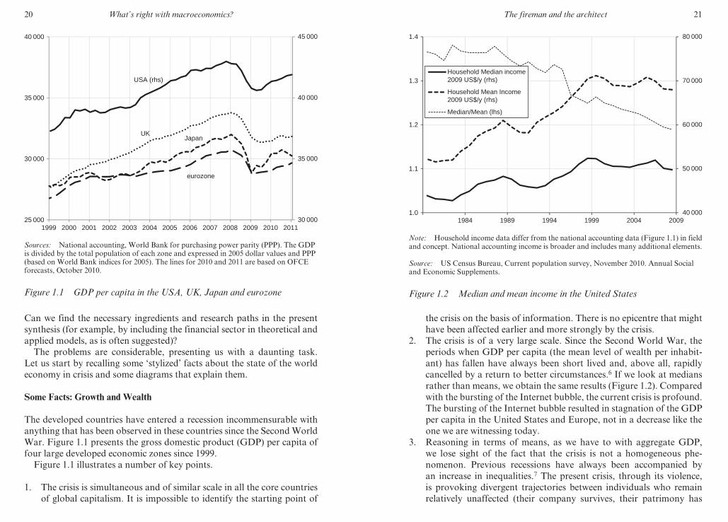
The developed countries have entered a recession incommensurable with
anything that has been observed in these countries since the Second World
War. Figure 1.1 presents the gross domestic product (GDP) per capita of
four large developed economic zones since 1999.
Figure 1.1 illustrates a number of key points.
1. The crisis is simultaneous and of similar scale in all the core countries
of global capitalism. It is impossible to identify the starting point of
30 000
35 000
40 000
45 000
25 000
30 000
35 000
40 000
USA (rhs)
UK
eurozone
Japan
1999 2000 2001 2002 2003 2004 2005 2006 2007 2008 2009 2010 2011
Sources: National accounting, World Bank for purchasing power parity (PPP). The GDP
is divided by the total population of each zone and expressed in 2005 dollar values and PPP
(based on World Bank indices for 2005). The lines for 2010 and 2011 are based on OFCE
forecasts, October 2010.
Figure 1.1 GDP per capita in the USA, UK, Japan and eurozone
M3014 - SOLOW TEXT.indd 20 21/11/2012 13:03
The fireman and the architect 21
the crisis on the basis of information. There is no epicentre that might
have been affected earlier and more strongly by the crisis.
2. The crisis is of a very large scale. Since the Second World War, the
periods when GDP per capita (the mean level of wealth per inhabit-
ant) has fallen have always been short lived and, above all, rapidly
cancelled by a return to better circumstances.6 If we look at medians
rather than means, we obtain the same results (Figure 1.2). Compared
with the bursting of the Internet bubble, the current crisis is profound.
The bursting of the Internet bubble resulted in stagnation of the GDP
per capita in the United States and Europe, not in a decrease like the
one we are witnessing today.
3. Reasoning in terms of means, as we have to with aggregate GDP,
we lose sight of the fact that the crisis is not a homogeneous phe-
nomenon. Previous recessions have always been accompanied by
an increase in inequalities.7 The present crisis, through its violence,
is provoking divergent trajectories between individuals who remain
relatively unaffected (their company survives, their patrimony has
1.0
1.1
1.2
1.3
1.4
40 000
50 000
60 000
70 000
80 000
200920041999199419891984
Household Median income2009 US$/y (rhs)
Household Mean Income2009 US$/y (rhs)
Median/Mean (lhs)
Note: Household income data differ from the national accounting data (Figure 1.1) in field
and concept. National accounting income is broader and includes many additional elements.
Source: US Census Bureau, Current population survey, November 2010. Annual Social
and Economic Supplements.
Figure 1.2 Median and mean income in the United States
M3014 - SOLOW TEXT.indd 21 21/11/2012 13:03

22 What’s right with macroeconomics?
not depreciated, their job is safe) and others who are caught up in
spirals that amplify the initial shock (loss of job, sale of real estate or
financial capital at the most unfavourable moment, and so on). Table
1.1 presents the variations in unemployment, an indicator that reveals
some of the heterogeneity.
Figure 1.3 shows an aspect of the crisis that is complementary to the one
we have observed for flows – the impact on stocks. The concept used here
is US household wealth. Because of the way the accounts of US wealth
are calculated, this concept has the advantage of summarizing the loss of
wealth incurred by economic agents. The calculation involves consolidat-
ing the variations in assets and liabilities in the accounts of US households.
Ultimately, along with government and foreign investors, households are
the owners of variations in assets in the US economy.
Figure 1.3 gives us an idea of the magnitude of the impact that the crisis
has had on wealth. Adding together financial and real estate wealth net
of debt, we can see that the crisis has caused US households to lose the
equivalent of 150 per cent of their income. This order of magnitude is
similar to the loss of wealth that occurred when the Internet bubble burst,
but it is also similar to the gain in financial wealth caused by the forma-
tion of that bubble or to the gain in wealth produced during the period
before the crisis8 (nevertheless, the post-2007 crisis appears to be more
serious, and the next one may well be worse). In the space of just a few
years, the average US household saw their wealth magically increase by
the equivalent of one and a half year’s income. This allowed them, for
example, to stop saving for their retirement, since the returns on capital
already saved were sufficient to maintain their standard of living. When
Table 1.1 Unemployment and economic activity in the crisis of 2008
Variation between
2010q2 and 2008q1
FRA GER ITA JPN USA UK SPA
GDP/habitant
(in %)
−3.5 −2.3 −7.1 −4.5 −3.2 −5.8 −6.0
GDP (in %) −2.2 −2.7 −5.6 −4.3 −1.1 −4.5 −4.6
Unemployment 12.1 −0.6
(11.3)*
12.2 11.4 14.9 12.6 110.8
Note: *Unemployment figure including, for Germany, partial unemployment.
Source: National statistics institutes (INSEE of France, Dstatis of Germany, Istat of
Italy, and so on); calculations by the author.
M3014 - SOLOW TEXT.indd 22 21/11/2012 13:03
The fireman and the architect 23
the capital suddenly depreciated, on the other hand, they suffered a similar
loss, leaving many households in a troublesome situation.
It is impossible to establish a detailed diagnosis of the impact of the infla-
tion of wealth on the different fractiles of wealth or income. Nevertheless,
and especially for the crisis of 2008, the fact that both real estate and finan-
cial wealth are affected suggests that the impact is not concentrated on the
wealthiest. The financialization of modern developed economies has resulted
in practically every household owning some form of wealth. Thus, home
ownership rates are high, particularly when one only considers adult popu-
lations engaged in active and family life. It is facilitated by broad access to
credit. Second, pension savings systems have become important in the devel-
oped countries, accumulating assets of the order of 100 per cent in the United
States or the United Kingdom, to name but two. In this respect, France is
very atypical, with very weak development of pension funds, which protected
it from the sharp depreciation of assets experienced during the crisis.
Radical Uncertainty, Positive Feedback Loops, Instability
These elements illustrate the tremendous tension generated by the use of
financial markets. On one side, households make savings equal to several
0%
100%
200%
300%
400%
500%
600%
700%
1952 1957 1962 1967 1972 1977 1982 1987 1992 1997 2002 2007
Net housing wealth
Other physical assets
As a % share of household income (FoF 3/2011)
Net financial wealth
Source: Flow of Funds, Federal reserve statistical release, March 2011; calculations by the
author.
Figure 1.3 US household wealth
M3014 - SOLOW TEXT.indd 23 21/11/2012 13:03
24 What’s right with macroeconomics?
times their annual income,9 and these savings are entrusted to the finan-
cial system. On the other side, the financial system, from the banks to the
pension funds by way of every imaginable type of intermediary, uses these
savings to generate a return by lending them to those who need credit.
These are households, governments, local authorities and private enter-
prise. In any event, the aim is to match the need for secure, long- term,
liquid saving with the need for risky, short- term, illiquid credit. It is also
important to ensure the liquidity of the whole system. This transforma-
tion of the risk is quite easy when it involves meeting the financing needs
of a developed state. In that case, the need for credit is expressed over the
long term with a high level of security against default. It is therefore easy
to match this credit need with a need for saving that has similar character-
istics. Ensuring liquidity is also easy, as long as a secondary market exists
for trading in the public debt bonds, which is the case for large states or
for bonds issued in euros.
The difficulty of the operation is comparable when it comes to financing
the credit needs of households. These mainly concern the purchase of real
estate and therefore have similar characteristics to household saving: fairly
high security and long- term horizons.10
The transformation of risk is intrinsically more delicate for the private
sector, however. The attention that has been focused on sub- prime lending
as the factor that triggered the Great Recession sometimes overshadows
the consequences of a sudden, sharp fall in productive assets. And yet
the transformation of long- term, risk- averse savings into the financing of
risky activity is problematic. If the markets are efficient, then the volatil-
ity in the value of productive assets comes from the fact that the activities
involved are risky, but the absence of bias in the aggregate value of pro-
ductive assets allows one to reduce the risk to zero by using the law of large
numbers. This is what the capital asset pricing model (CAPM) and the
Black–Scholes formula do: diversifying to create a risk- free asset, however
abstract. But this is where the illusion comes into play, since there is no
guarantee that there is not a general bias in the value of assets. In fact,
the data have indicated the exact opposite since the end of the 1990s. The
value of the assets owned by US households is known to the nearest 150
per cent of income!
Faced with such aggregate uncertainty, which is persistent enough over
time to allow the formation of bubbles, no financial instrument can satisfy
the need for transformation. The financial system or the households are
then exposed to the failure of valuation, to that discounted value of future
returns that the financial markets cannot predict.
The financialization of economies has consisted in the transfer of more
and more operations of transformation of savings from isolated, special-
M3014 - SOLOW TEXT.indd 24 21/11/2012 13:03
The fireman and the architect 25
ized institutions towards a general model of market finance. So it was
that housing finance moved from a closed circuit (households borrowing
from the housing savings of households, collected by paragovernmental
institutions) towards an open circuit (the securitization of mortgages), and
intermediation by banks was pushed out by direct or structured circuits
(such as private equity). At the same time, contributory pension schemes
were ‘complemented’ by funded pension plans. In fact, this involved
substitution rather than topping- up.
In this trend, ever greater masses of capital are moving about, heighten-
ing the general risk and becoming ever more dependent on an accurate
valuation of the productive assets. At the same time, investors have been
becoming more diversified. Instead of experienced investors financing
risky productive activities with a high level of direct involvement, a whole
category of investors has emerged whose sole concern is not to have any
concerns, prepared to turn a blind eye to the management of their pension
savings so long as they are promised a modest but secure return.
National compromises may impose a ratchet effect on this system. By
promoting funded pension plans (which appeared, during a felicitous
period, to give particularly good returns), and thereby avoiding the poten-
tial difficulties of trying to balance their contributory pension schemes,
governments guaranteed the promise made to savers. That promise was
that their savings would be worth something in a few decades and that in
the meantime, they would give real positive returns. To achieve that, it is
not enough for capital markets to produce fair value; they must produce
constant growth in value. And for that reason, governments prefer the
formation of bubbles to any other solution.
This is quite a terrible trap. In the name of market efficiency, on the
grounds that the returns obtained were better than those of contribu-
tory systems, the developed world has nurtured a financial sector that is
incapable of keeping its promises, quite simply because those promises
have no meaning. When disaster strikes, the only solution is to keep the
house of cards standing as long as possible, whatever the cost. The bubble
suits everyone; uncertainty hides the fact that the promises are untenable;
the positive feedback loops interact and generate instability on a macr-
oeconomic scale. When, in addition, learned economists lend their moral
and intellectual support to the edifice, one would have to be crazy to refuse
this dream.
Debt Deflation: ‘Fisher’s Nightmare’
The entry into recession manifests itself in a fall in economic activity and
in the value of assets and a rise in unemployment. Unsurprisingly, this
M3014 - SOLOW TEXT.indd 25 21/11/2012 13:03

26 What’s right with macroeconomics?
causes a slowdown in inflation. Unfortunately, the rise in oil and food
prices has masked this evolution in the price indices.11 The underlying
indices, presented in Figure 1.4, are unequivocal.
In all the economic zones considered here, the entry into recession has
been accompanied by a reduction in underlying inflation of about half
of 1 per cent per year. At that rate, the United States and the eurozone
would enter deflation in 2012 while Japan would sink once again. The
fact that deflation can appear despite the expansionist monetary policy
being pursued (low interest rates and ‘unconventional’ policies) suggests
that the system is caught in a liquidity trap, where this expansionist mon-
etary policy is no longer effective. In the 1930s, it was called ‘pushing on
a string’. Krugman (1998) gives a more modern definition of the liquidity
trap: it is a situation where the real short- term interest rate necessary to
stimulate the economy would have to be negative. And yet expectations of
inflation (or rather, of deflation) make it impossible to expect a negative
real rate. The only solution is to increase expectations of inflation. In a
situation of creeping deflation, this is indeed very much like pushing on a
string.
–2
–1
0
1
2
3
Japan
USA
eurozone
199919981997 2000 2001 2002 2003 2004 2005 2006 2007 2008 2009 2010
Source: Nation al statistical institutes (INSEE of France, Dstatis of Germany, Istat of
Italy, and so on). Quarterly price indices excluding volatile products (energy and food) in
annual growth rhythm.
Figure 1.4 Underlying inflation for the large developed countries
M3014 - SOLOW TEXT.indd 26 21/11/2012 13:03
The fireman and the architect 27
Entering deflation would have disastrous consequences. This is the
process of debt deflation described by Irving Fisher (1933). One notable
difference from the 1930s is the level of financial debts that agents have
accumulated. Figure 1.5 shows the components of US debt as a percentage
of GDP. The figures for the other developed economic zones are similar.
For debts at fixed nominal rates of interest, deflation produces an
increase in the real rate. For debts at variable rates, it has no impact. It is
hard to know the exact proportions of fixed- and variable- rate debts, but
we do know that a large quantity (almost all) are practically fixed rate.
The rise in the cost of debts will force agents to massively reduce their
debts. This process will exacerbate the recession and fuel deflation. When
the rhythm of deflation falls below - 2 per cent per year, real rates are at
a minimum of 2 per cent. With each step deeper into deflation, real rates
increase.
The process of deflation can accelerate if defaults occur rather than
agents being prompted to pay back their debts as fast as possible. In a
highly financialized system, the expectation of default can lead to an
immediate hike in risk premiums, thereby producing the default. In this
case, expectations are self- fulfilling and the economic system becomes
0
50
100
150
200
250
300
350
400
Households
Non-financial business
Government (federal+local)
Financial sector
Rest of the world
1952 1957 1962 1967 1972 1977 1982 1987 1992 1997 2002 2007
Source: Flow of Funds, Federal reserve statistical release, September 2010, calculations
by the author.
Figure 1.5 Components of US debt as a percentage of GDP
M3014 - SOLOW TEXT.indd 27 21/11/2012 13:03

28 What’s right with macroeconomics?
more unstable. The Greek crisis provides a good illustration of these
instabilities.
Fisher considered debt deflation to be the driving force behind the
Great Depression. The state of the developed world’s debts in deflation is
‘Fisher’s nightmare’.
CONCLUSION: A PARADIGM SHIFT?
The crisis represents a profound violation of the world view structured
by the five neutralities. How can one determine a permanent income
in such an event? How can one imagine that companies go through the
crisis independently of their balance sheet structure? How can one believe
in Ricardian equivalence when governments are embarking on massive
stimulus packages? How can one uphold the existence of ‘natural’ or equi-
librium unemployment, supposed to be an attractor of economic dynam-
ics when unemployment is persistently above 10 per cent in the developed
countries? And how can one maintain the hypothesis of market efficiency
when the hegemony of markets over the organization of the globalized
economy has led to unprecedented disaster?
It becomes impossible to defend these neutralities in the face of such
overwhelming facts. The crisis has shown us two things: uncertainty is
radical and the heterogeneity of agents plays a central role. These two ele-
ments interact, and one cannot analyse the economy without taking into
consideration the nature of expectations.
It is not that economic agents are irrational, it is the definition of ration-
ality habitually used in modern macroeconomics that completely miscon-
strues the universe in which we live and move. If there was no uncertainty
about the future, we could all form the same expectation, corresponding a
priori to the aggregate result a posteriori. Because the future is irreducible
and no market can diminish that uncertainty, expectations are heterogene-
ous and imperfect. This heterogeneity comes on top of that of the agents
and of the information they possess or are capable of acquiring.
In a universe of uncertainty and heterogeneity, institutions play a role in
reducing uncertainty; they are islands of stability. They provide a form of
coordination between isolated and lost economic agents. Institutions are
a means to reacting to new or uncontrollable situations. They are a means
of reducing the radical uncertainty that we face. They are also endogenous
to the economic process, conceived and accepted with a precise objective,
as a solution to a problem.
Modern macroeconomics appears to disregard all that, often on the
grounds of one sole argument: moral hazard. If architects relied on the
M3014 - SOLOW TEXT.indd 28 21/11/2012 13:03
The fireman and the architect 29
presence of fire fighters, then they might well design towers that are less
safe. When individuals are certain that someone will intervene to save
them in the event of disaster, they no longer run the risk of being punished
for their mistakes and they behave recklessly and irresponsibly. Ensuring
that everyone is responsible for their actions is commendable, but there
exists a level of disaster where that consideration becomes secondary. That
is all the more so since it is perfectly possible to punish those responsible
after the firemen have done their work (although this is easier said than
done, as we have seen in the crisis).
Neither methodological individualism nor the concept of rationality
should be abandoned. On the other hand, as Akerlof insists, it is urgent
that rationality be defined in a way that is both convincing and enlighten-
ing about how economies function, instead of continuing to entertain a
misleading conception.
It would be presumptuous to call for a paradigm shift. And yet current
lines of research in macroeconomics, as represented by the new synthesis,
are deeply challenged by the natural experiment of the crisis. While await-
ing a better explanation of how economies work, we can only express our
dissatisfaction.
NOTES
1. I would like to thank the organizers of the conference held by the Cournot Centre on
2–3 December 2010, especially Therrese Goodlett and Lucia Scharpf, Robert Solow
and Jean- Philippe Touffut, and the other participants, in particular Robert Boyer,
Jean- Bernard Chatelain, Giovanni Dosi, Bernard Gazier, Robert Gordon and Xavier
Ragot. Their remarks were invaluable to me in writing this text. Thanks also to friends
Philippe Daulouède, Guillaume Daudin and Joël Maurice for re- reading the text,
whose remaining shortcomings are entirely mine.
2. Here, the term ‘long run’ is deliberately vague. It means that inevitably, after a certain
time, unemployment will have no influence on inflation. The trade- off between infla-
tion and unemployment is therefore an illusion, or the result of temporary frictions or
imperfections. In a reasonable world, that will not last very long, and the long run may
be no more than a few months.
3. It is difficult to see unemployment as a product of nature. Unemployment presupposes
a non- autarkic, wage- earning society. The qualification ‘natural’ unemployment is
therefore questionable. Beyond the semantic detail, it is interesting to note that it was
through natural unemployment and the concept of equilibrium unemployment that
‘structural’ reasoning was developed, bringing into play institutions such as unemploy-
ment insurance, employee bargaining power and the market power of employers or
employees. This idea appeared to be very useful, since the cyclical (macroeconomic) and
the structural only meet orthogonally, without having an effect on each other.
4. ‘Mainstream’ should be understood as descriptive and non- normative. The mainstream
approach is rich and varied, founded on a common base (of which the five neutrali-
ties constitute a matrix) from which it has developed along many different paths, with
methodological additions that are sometimes far removed from the core.
5. In other words, making propositions (predicates) that can be refuted and then
M3014 - SOLOW TEXT.indd 29 21/11/2012 13:03

30 What’s right with macroeconomics?
conducting reproducible, controlled experiments to test those predicates. As long as
no experiment refutes the proposition, it is considered acceptable (that is to say, true in
the naive sense of the word). Macroeconomics is characterized by statements that are
generally not refutable.
6. This point is not visible in Figure 1.1. Long- run analyses show that the post- war period
was one of strong and stable growth, compared, for example, with the nineteenth
century or, obviously, the first half of the twentieth century.
7. One can even suppose that these inequalities are random and in no way related to
a form of efficiency (in the sense of John Rawls, 1971) that might give them some
legitimacy.
8. In changes in wealth, one can distinguish between those resulting from savings flows
(net of the consumption of fixed capital) and those resulting from price variations.
Unsurprisingly, a huge proportion of the recent evolution of wealth is due to price
changes.
9. To ensure a relatively constant standard of living, it is necessary to save approxi-
mately 7 times one’s annual income (based on 40 years’ working, 20 years’ retire-
ment, 2 per cent of real return, retirement income equal to 80 per cent of net income,
from savings or social security contributions). On average, in the United States, real
estate wealth is equivalent to 2 to 3 times annual end- of- career income, and financial
wealth around 1 to 2 times annual income. The remainder is made up by contributory
pension schemes.
10. Sub- prime lending is a striking exception to this general rule. Aside from sub- prime
lending, and as long as we restrict ourselves to stable populations with well identified
incomes, without counting on capital gains to ensure the solvency of the whole system,
mortgage lending is a risk- free activity, subject to hazards that are well measured and
well controlled.
11. It could be argued that the rise in oil and food prices is the symptom of a situation
of scarcity and is in itself a factor of inflation. In that case, it would be better to look
at the complete indices. Price rises due to scarcity do not necessarily turn into infla-
tion, however, and may simply cause a change (albeit substantial) in relative prices.
The underlying indices filter out these components. If these indices rise, they are the
symptom of a general rise in prices, in a spiral of prices, costs and wages. The scarcity
of certain products may be the triggering factor. It has been shown that the underlying
indices are better predictors of trends over a few quarters than price indices. This tends
to confirm that scarcity is not a sufficient condition for inflation.
REFERENCES
Acemoglu, Daron (2009), ‘The crisis of 2008: structural lessons for and from economics’, CEPR Policy Insight, 28, available at: http://www.cepr.org/pubs/policyinsights/PolicyInsight28.pdf, accessed 24 August 2011.
Akerlof, George (2007), ‘The missing motivation in macroeconomics’, American Economic Review, 97(1), 5–36.
Barro, Robert (1974), ‘Are government bonds net wealth?’, The Journal of Political Economy, 82(6), 1095–117.
Bernanke, Ben S. (2004), ‘The great moderation’, remarks by Governor Ben S. Bernanke at the meetings of the Eastern Economic Association, Washington, DC, 20 February, available at: http://www.federalreserve.gov/boarddocs/speeches/2004/20040220/default.htm, accessed 24 August 2011.
Blanchard, Olivier (2009), ‘The state of macro’, Annual Review of Economics, 1(1), January, 209–28.
M3014 - SOLOW TEXT.indd 30 21/11/2012 13:03
The fireman and the architect 31
Blanchard, Olivier and John Simon (2001), ‘The long and large decline in US output volatility’, Brookings Papers on Economic Activity, 32(1), 135–74, avail-able at: http://www.brookings.edu/~/media/Files/Programs/ES/BPEA/2001_1_bpea_papers/2001a_bpea_blanchard.pdf, accessed 24 August 2011.
Boyer, Robert (2008), ‘History repeating for economists: an anticipated finan-cial crisis’, Cournot Centre Prisme Series, no. 13, available at: http://www.centre- cournot.org/index.php/2008/11/26/history- repeating- for- economists- an- anticipated- financial- crisis, accessed 24 August 2011.
Diamond, Peter (1982), ‘Demand management in search equilibrium’, Journal of Political Economy, 90, 881–94.
Fama, Eugene F. (1970), ‘Efficient capital markets: a review of theory and empiri-cal work’, Journal of Finance, 25(2), July, 383–417.
Fisher, Irving (1933), ‘The debt- deflation theory of great depressions’, Econometrica: Journal of the Econometric Society, 1(4), 337–57.
Frydman, Roman and Michael D. Goldberg (2007), Imperfect Knowledge Economics, Princeton, NJ: Princeton University Press.
Galbraith, James K. (2009), ‘Who are these economists, anyway?’, Thought and Action, Fall, pp. 85–97.
Kindleberger, Charles (1996), Manias, Panics, and Crashes: A History of Financial Crises, 3rd edn, 1st edn published in 1978, New York: Basic Books.
Kirman, Alan P. (1992), ‘Whom or what does the representative individual rep-resent?’, Journal of Economic Perspectives, 6(2), Spring, 117–36, available at: http://www.jstor.org/stable/2138411, accessed 16 June 2011.
Krugman, Paul (1998), ‘It’s baaack: Japan’s slump and the return of the liquidity trap’, Brookings Papers on Economic Activity, 1998(2), 137–205.
Krugman, Paul (2000), ‘How complicated does the model have to be?’, Oxford Review of Economic Policy, 16(4), December, 33–42.
Krugman, Paul (2009a), The Return of Depression Economics, New York: W.W. Norton.
Krugman, Paul (2009b), ‘How did economists get it so wrong?’, New York Times Magazine, available at: http://www.nytimes.com/2009/09/06/magazine/06Economic- t.html, accessed 24 August 2011.
Leijonhufvud, Axel (2009), ‘Macroeconomics and the crisis: a personal appraisal’, CEPR Policy Insight, 41, available at: http://www.cepr.org/pubs/policyinsights/PolicyInsight41.pdf, accessed 24 August 2011.
Lucas, Robert E. (1988), ‘What economists do’, Journal of Applied Economics, Universidad del CEMA, 0, pp. 1–4, May.
Lucas, Robert and Thomas Sargent (1978), ‘After Keynesian macroeconom-ics’, in Federal Reserve Bank of Boston, After the Phillips Curve: Persistence of High Inflation and High Unemployment, proceedings of conference held in June 1978, The Federal Reserve Bank of Boston Conference Series, no. 19, pp. 49–72.
McCloskey, Donald N. (1983), ‘The rhetoric of economics’, Journal of Economic Literature, 21(2), 481–517.
Milanovic, Branko (2006), ‘Global income inequality’, World Economics, 7(1), 131–57, available at: http://www.nupi.no/layout/set/print/content/download/3901/57934/version/5/file/GlobalIncomeInequality.pdf, accessed 21 June 2011.
Minsky, Hyman P. (1986), Stabilizing an Unstable Economy, New Haven, CT, and London: Yale University Press.
Modigliani, Franco and Merton Miller (1958), ‘The cost of capital, corporation
M3014 - SOLOW TEXT.indd 31 21/11/2012 13:03
32 What’s right with macroeconomics?
finance and the theory of investment’, American Economic Review, 48(3), 261–97.
Rawls, John (1971), Theory of Justice, Cambridge, MA: Belknap Press of Harvard University Press.
Solow, Robert (2010), ‘Building a science of economics for the real world’, pre-pared statement for the US House Committee on Science and Technology Subcommittee on Investigations and Oversight, 20 July.
Stiglitz, Joseph E. (2009), ‘The current economic crisis and lessons for economic theory’, Eastern Economic Journal, 35(3), 281–96.
Stiglitz, Joseph E. and Bruce Greenwald (2003), Toward a New Paradigm in Monetary Economics, Cambridge, UK: Cambridge University Press.
Summers, Lawrence H. (1991), ‘The scientific illusion in empirical macroeconom-ics’, Scandinavian Journal of Economics, 93(2), 129–48, available at: http://www.jstor.org/stable/3440321, accessed 21 June 2011.
Syll, Lars P. (2010), ‘What is (wrong with) economic theory’, Real World Economics Review, no. 54, August, pp. 23–57.
Timbeau, Xavier (2011), ‘Solidarité intergénérationnelle et dette publique’, Revue de l’OFCE, 116(1), 191–212.
Wyplosz, Charles (2009), ‘Macroeconomics after the crisis. Dealing with the Tobin Curse’, Walter Adolf Jöhr Lecture 2009, Contributions to Economics, no. 10, June, Institute of Economics, University of St Gallen.
M3014 - SOLOW TEXT.indd 32 21/11/2012 13:03
33
2. Model comparison and robustness: a proposal for policy analysis after the financial crisis1
Volker Wieland
INTRODUCTION
In the aftermath of the financial crisis, the state of macroeconomic model-
ling and the use of macroeconomic models in policy analysis have come
under heavy criticism. Media and other commentators have criticized
macroeconomists for failing to predict the Great Recession of 2008–09,
or at least for failing to provide adequate warning of the risk of such
a recession. Practitioners have attributed this failure to academic and
central bank researchers’ love of a particular modelling paradigm. They
blame so- called dynamic stochastic general equilibrium (DSGE) models
for misdirecting the attention of policy makers. Indeed, even some well-
known academics- cum- bloggers have published scathing commentaries
on the current state of macroeconomic modelling. On 3 March 2009,
Willem Buiter wrote on the Financial Times blog,2 ‘the typical graduate
macroeconomics and monetary economics training received at Anglo-
American universities during the past 30 years or so, may have set back
by decades serious investigations of aggregate economic behaviour and
economic policy- relevant understanding’. This view was echoed by Nobel
Laureate Paul Krugman on 11 June 2009 in the weekly Economist, ‘Most
work in macroeconomics in the past 30 years has been useless at best and
harmful at worst’.
Against this background, this chapter aims to develop a more con-
structive proposal for how to use macroeconomic modelling – whether
state- of- the- art or 1970s vintage – in practical policy design. It is written
in the vein of the 1992 call for a pluralistic and rigorous economics by
leading economists. The undersigned – among them Nobel Laureates
Paul Samuelson and Franco Modigliani – were concerned with ‘the threat
to economic science posed by intellectual monopoly’ and pleaded for ‘a
new spirit of pluralism in economics, involving critical conversation and
M3014 - SOLOW TEXT.indd 33 21/11/2012 13:03

34 What’s right with macroeconomics?
tolerant communication between different approaches.’3 It is in that spirit
that I propose a systematic comparative approach to macroeconomic
modelling with the objective of identifying policy recommendations that
are robust to model uncertainty.4 This approach is open to a wide variety
of modelling paradigms.
Scientific rigour demands a level playing field on which models can
compete. Rather than using rhetoric to dismiss competing approaches,
emphasis should be placed on empirical benchmarks that need to
be satisfied by the models in order to stay in the race. For example,
macroeconomic models used for monetary policy could be required to
be estimated to fit the empirical dynamics of key time series, such as
output, inflation and nominal interest rates. Models should be able to
provide answers to policy makers’ typical questions, such as what is the
effect of an unanticipated increase (or decrease) in the central bank’s
operating target for the money market rate, or of an unanticipated
temporary increase (or decrease) in government spending or transfers?
Another common concern is the degree of output, inflation and interest
rate volatility and persistence predicted by the models under different
policy rules. New modelling approaches may offer more sophisticated
explanations of the sources of the Great Recession of 2008–09 and carry
the promise of improved forecasting performance. This promise should
be put to a test rather than presumed. Estimated models could be com-
pared along their relative real- time forecasting performance, in particu-
lar during periods of great change, such as recessions and recoveries. An
example of such a model competition is given by Volker Wieland and
Maik Wolters (2010).
Macroeconomic data, however, are unlikely to provide sufficient testing
grounds for selecting a single, preferred model for policy purposes. Instead,
policy recommendations should be made robust to model uncertainty. In
particular, the robustness of policy prescriptions can be improved by
introducing them in multiple, competing models and comparing perform-
ance across models according to established target criteria. Policy makers
continue to require models and are aware of the need for robustness. In
November 2010, the European Central Bank President expressed these
needs very clearly:
We need macroeconomic and financial models to discipline and structure our judgemental analysis. How should such models evolve? The key lesson I would draw from our experience is the danger of relying on a single tool, methodol-ogy or paradigm. Policymakers need to have input from various theoretical perspectives and from a range of empirical approaches. Open debate and a diversity of views must be cultivated – admittedly not always an easy task in an institution such as a central bank. We do not need to throw out our DSGE
M3014 - SOLOW TEXT.indd 34 21/11/2012 13:03
Model comparison and robustness 35
and asset- pricing models: rather we need to develop complementary tools to improve the robustness of our overall framework.5
Macroeconomic model comparison projects have already helped
produce some very influential insights for practical policy making. For
example, John B. Taylor (1993a) credits the comparison project organized
by the Brookings Institution and summarized in Ralph Bryant et al. (1993)
as the crucial testing ground for what later became known as the Taylor
rule for monetary policy. More recently, the International Monetary
Fund (IMF) organized a large- scale model comparison exercise in order
to evaluate the likely consequences of temporary fiscal stimulus measures
(see Coenen et al., 2012). Such model comparisons have been, neverthe-
less, infrequent and costly, because they require the input of many teams
of researchers and multiple meetings to obtain a limited set of comparative
findings.
To remedy this situation, Volker Wieland et al. (2009) have imple-
mented a new approach to model comparison that enables individual
researchers to conduct such comparisons easily, frequently, at low cost
and on a large scale. This methodology comes with a model archive that
includes many well- known empirically estimated models of business- cycle
dynamics. These models can be used to evaluate the performance of mac-
roeconomic stabilization policies. A computational platform that allows
straightforward comparisons of models’ implications using MATLAB
and DYNARE6 software is available online to download.7 Researchers
can easily include new models in the database and compare the effects of
novel extensions to established benchmarks.
Our proposal is to use this comparative approach systematically in
order to organize a pluralistic, yet rigorous and productive communica-
tion between competing modelling paradigms in macroeconomics. So
far, the model database contains small- , medium- and large- scale macro-
economic models of different vintages and methodological traditions.
The first release of November 2010 covers 38 models, including many
state- of- the- art New-Keynesian DSGE models, but also earlier vintage
New- Keynesian models with rational expectations and nominal rigidities,
as well as some models that offer a more traditional Keynesian- style per-
spective on macroeconomic fluctuations with largely backward- looking
dynamics. The model database and the computational platform for model
comparison provide a level playing field that is open to new entrants.
Going forward, we propose to cover as many competing modelling para-
digms as possible, so as to compare models’ empirical implications in a
systematic fashion, and to search for policy prescriptions that are robust
along relevant dimensions of model uncertainty.
M3014 - SOLOW TEXT.indd 35 21/11/2012 13:03

36 What’s right with macroeconomics?
The next section briefly describes the comparison methodology and
gives an overview of the models available in the database. It also outlines a
list of competing modelling paradigms that promise improvements in our
understanding of macroeconomic dynamics. In future work, they should
be compared to those approaches that have received the most attention
in recent years. The third section gives an example of a demanding test of
comparative model performance, namely the real- time forecasting evalu-
ation of a range of models relative to those of experts in the last five US
recessions, conducted by Wieland and Wolters (2010). The next section
reviews findings from recent comparative studies regarding the impact of
fiscal stimulus packages and reports estimates of the impact of govern-
ment transfers in selected models. The final section concludes.
MODEL COMPARISON
The six older comparison projects reported in Bryant et al. (1988), Bryant
et al. (1989), Klein (1991), Bryant et al. (1993), Taylor (1999), Hughes-
Hallett and Wallis (2004), as well as the recent IMF exercise by Coenen
et al. (2012) have all involved multiple teams of researchers, each team
working only with one or a small subset of available models. The approach
by Wieland et al. (2009), on the other hand, is meant to provide users easy
access to the complete set of models considered in a comparison exercise.
Furthermore, users should find it fairly straightforward to integrate their
own models. To this end, Wieland et al. (2009) present a formal exposition
of their comparative methodology. Taylor and Wieland (2012) use the
model database to compare three well- known models of the US economy
and analyse the robustness of simple monetary policy rules.
A general class of non- linear dynamic stochastic macroeconomic models
is augmented with a space of common comparable variables, parameters
and shocks. Augmenting models in this manner is a necessary precondition
for a systematic comparison of particular model characteristics. Given a
space of common variables and parameters, one can define common
policy rules as model input and produce comparable objects as model
output. These objects are also defined in terms of common variables,
parameters and shocks. Examples for such objects are impulse response
functions, autocorrelation functions and unconditional distributions of
key macroeconomic aggregates.
The space of common variables, parameters and policy rules comprises
only a subset of each model’s variables, parameters and equations. Most
model- specific equations remain unchanged. Only the model- specific
policy rules are replaced with common policy rules that express policy
M3014 - SOLOW TEXT.indd 36 21/11/2012 13:03
Model comparison and robustness 37
variables as functions of common variables and parameters. Nevertheless,
a new set of definitional equations needs to be added to each model. These
definitional equations define the common variables in terms of model-
specific variables. Once each model is augmented with the appropriate
definitional equations and the common policy rules, it is ready for com-
parative exercises. For a formal exposition of the procedure for integrat-
ing new models, see Wieland et al. (2009). Several examples are carried out
step- by- step in that paper. A detailed documentation of the augmented
model files is also provided.
A Model Database
In the following, I give a brief overview of the model archive that is
available with the comparison software. This database includes many
well- known, empirically- estimated macroeconomic models that may be
used for quantitative analysis of monetary and fiscal stabilization poli-
cies. It contains estimated and calibrated models of the US economy and
the euro area. There are also a number of small open- economy models
of countries such as Canada, Chile and Brazil. Finally, it also includes
several multi- country models that cover industrialized economies. The
models, made available in the first release as of November 2010, are listed
in Table 2.1.
Most models could be classified as New Keynesian, because they incor-
porate rational expectations, imperfect competition and wage or price
rigidities. A subset of the models could be characterized as monetary
business cycle models where all behavioural equations are derived in a
completely consistent manner from the optimization problems of rep-
resentative households and firms. Many authors use the term ‘dynamic
stochastic general equilibrium’ (DSGE) model to refer to this particular
class of model. Thus, the database offers interesting opportunities for
comparing policy implications of this class of model to a broader set of
empirically estimated, dynamic, stochastic, economy- wide macro models.
While most of the models assume that market participants form
rational, forward- looking expectations, we have also included some
models that assume little or no forward- looking behaviour.8 Comparative
analysis of these classes of models will be useful to evaluate recently voiced
criticisms that the newer models have been rendered invalid by the global
financial crisis.
The models are grouped into five categories in Table 2.1. The first
category includes small, calibrated versions of the basic New- Keynesian
DSGE model. These models concentrate on explaining output, inflation
and interest- rate dynamics. Some of them are calibrated to US data. The
M3014 - SOLOW TEXT.indd 37 21/11/2012 13:03

38 What’s right with macroeconomics?
model taken from Clarida et al. (2002) is a two- country version of this type
of model.
The second category covers estimated models of the US economy. It
includes small models of output, inflation and interest- rate dynamics, such
as Fuhrer and Moore (1995) and Rudebusch and Svensson (1999). Other
models are of medium scale, such as Orphanides and Wieland (1998) or
the well- known models of Christiano, Eichenbaum and Evans (2005) and
Smets and Wouters (2007), which fully incorporate recent advances in
terms of microeconomic foundations. The database includes the version
of the Christiano–Eichenbaum–Evans model estimated by Altig et al.
(2005), because this version contains other economic shocks in addition
to the monetary policy shock studied by Christiano et al. (2005).9 We
have also included an additional version of the Altig et al. (2005) model
used in Taylor and Wieland (2012) that omits the cost channel of mon-
etary policy.10 The largest model of the US economy in the database is
the Federal Reserve’s FRB–US model of Reifschneider et al. (1999). We
have included a linearized version of this model with rational expectations
that was previously used in Levin et al. (2003), as well as two more recent
versions from 2008, one with rational expectations and one with adap-
tive expectations based on a reduced form vector- autoregression (VAR).
Federal Reserve economists Rochelle Edge, Michael Kiley and Jean-
Philippe Laforte (2010) have developed a new two- sector DSGE model
of the US economy that is also included in the database; a version of this
model is estimated in Wieland and Wolters (2010).
In addition, there are a number of smaller estimated models of the US
economy that offer new insights into the role of financial frictions in eco-
nomic fluctuations. Ioan Carabenciov et al. (2008), for example, augment
a simple backward- looking model with a measure of financial linkages
and frictions. Ferre De Graeve (2008) and Ian Christensen and Ali Dib
(2008) introduce constraints on firms’ financing following Ben Bernanke
et al. (1999) in a fully- fledged estimated DSGE model of the US economy.
These models provide an endogenous account of firms’ external finance
premium over the business cycle. Matteo Iacoviello (2005) includes the
housing sector in a DSGE model. The model of N. Gregory Mankiw and
Ricardo Reis (2007) deviates from the assumption of rational expectations
and allows for rational inattention. This mechanism introduces a role
for outdated expectations (or informational frictions) in business- cycle
dynamics. All these extensions of the standard DSGE framework were
accomplished before the financial crisis and could potentially be helpful in
rendering DSGE models more useful in explaining developments during
the crisis.
The third category in Table 2.1 covers estimated models of the euro- area
M3014 - SOLOW TEXT.indd 38 21/11/2012 13:03
Model comparison and robustness 39
Table 2.1 Models currently available in the database (November 2010)
1. SMALL CALIBRATED MODELS
1.1 NK RW97 Rotemberg and Woodford (1997)
1.2 NK LWW03 Levin et al. (2003)
1.3 NK CGG99 Clarida et al. (1999)
1.4 NK CGG02 Clarida et al. (2002)
1.5 NK MCN99cr McCallum and Nelson (1999), (Calvo–Rotemberg model)
1.6 NK IR04 Ireland (2004)
1.7 NK BGG99 Bernanke et al. (1999)
1.8 NK GM05 Gali and Monacelli (2005)
2. ESTIMATED US MODELS
2.1 US FM95 Fuhrer and Moore (1995)
2.2 US OW98 Orphanides and Wieland (1998) equivalent to MSR model
in Levin et al. (2003)
2.3 US FRB03 Federal Reserve Board model linearized as in Levin et al.
(2003)
2.4 US FRB08 2008 linearized version of Federal Reserve Board model
2.5 US FRB08mx 2008 linearized version of FRB model (mixed
expectations)
2.6 US SW07 Smets and Wouters (2007)
2.7 US ACELm Altig et al. (2005) (monetary policy shock)
US ACELt Altig et al. (2005) (technology shocks)
US ACELswm No cost channel as in Taylor and Wieland (2012) (mon.
pol. shock)
US ACELswt No cost channel as in Taylor and Wieland (2012) (tech.
shocks)
2.8 US NFED08 Based on Edge et al. (2007), version used for estimation in
Wieland and Wolters (2010)
2.9 US RS99 Rudebusch and Svensson (1999)
2.10 US OR03 Orphanides (2003)
2.11 US PM08 IMF projection model US, Carabenciov et al. (2008)
2.12 US PM08fl IMF projection model US (financial linkages),
Carabenciov et al. (2008)
2.13 US DG08 DeGraeve (2008)
2.14 US CD08 Christensen and Dib (2008)
2.15 US IAC05 Iacoviello (2005)
2.16 US MR07 Mankiw and Reis (2007)
3. ESTIMATED EURO AREA MODELS
3.1 EA CW05ta Coenen and Wieland (2005) (Taylor- staggered contracts)
3.2 EA CW05fm Coenen and Wieland (2005) (Fuhrer–Moore staggered
contracts)
3.3 EA AWM05 ECB’s area- wide model linearized as in Dieppe et al. (2005)
3.4 EA SW03 Smets and Wouters (2003)
3.5 EA SR07 Sveriges Riksbank euro area model of Adolfson et al.
(2007)
M3014 - SOLOW TEXT.indd 39 21/11/2012 13:03

40 What’s right with macroeconomics?
economy. Four of those models have been used in a recent study of robust
monetary policy design for the euro area by Keith Kuester and Volker
Wieland (2010): the medium- scale model of Smets and Wouters (2003),
two small models by Coenen and Wieland (2005) that differ by the type of
staggered contracts that induce inflation rigidity, and a linearized version
of the Area- Wide Model that was used at the European Central Bank
(ECB) for forecasting purposes. The latter was recently replaced by a new
DSGE model. In addition, we have included an estimated DSGE model
of the euro area recently developed at the Sveriges Riksbank (Adolfson et
al., 2007), and at the European Commission (Ratto et al., 2009). The latter
model was developed with a particular focus on the analysis of euro- area
fiscal policy.
The fourth category includes estimated and calibrated models of two
or more economies. Currently, the largest model in the database is the
estimated model of the G7 economies of Taylor (1993b). The estimated
model of Coenen and Wieland (2002) with rational expectations and price
rigidities aims to explain inflation, output and interest- rate dynamics and
spillover effects between the United States, the euro area and Japan. The
model of Laxton and Pesenti (2003) is a two- country model with extensive
microeconomic foundations calibrated to the economies of the euro area
and the Czech Republic. The Federal Reserve’s SIGMA model is similarly
rich in microeconomic foundations. The parameters in the two- country
Table 2.1 (continued)
3.6 EA QUEST3 QUEST III, model by DG- ECFIN EC, Ratto et al.
(2009)
4. ESTIMATED/CALIBRATED MULTI- COUNTRY MODELS
4.1 G7 TAY93 Taylor (1993b) model of G7 economies
4.2 G3 CW03 Coenen and Wieland (2002) model of USA, Euro area
and Japan
4.3 EACZ GEM03 Laxton and Pesenti (2003) model calibrated to Euro area
and Czech Republic
4.4 G2 SIGMA08 Federal Reserve’s SIGMA model from Erceg et al. (2008)
calibrated to the US economy and a symmetric twin
4.5 EAUS NAWM08 Coenen et al. (2008), New Area Wide model of Euro area
and USA
5. ESTIMATED MODELS OF SMALL OPEN ECONOMIES
5.1 CL MS07 Medina and Soto (2007), model of the Chilean economy
5.2 CA ToTEM10 ToTEM model of Canada, based on Murchison and
Rennison (2006), 2010 vintage
5.3 BRA SAMBA08 Gouvea et al. (2008), model of the Brazilian economy
M3014 - SOLOW TEXT.indd 40 21/11/2012 13:03
Model comparison and robustness 41
version of this model from Erceg et al. (2008) are calibrated to the US
economy and a symmetric twin. Finally, there is a two- country calibrated
version of the ECB’s new area- wide DSGE model as presented by Coenen
et al. (2008). This model also covers the US economy.
The fifth category of models covers small open- economy DSGE models
of Canada, Chile and Brazil. In addition to openness to trade and capital
flows, these models also consider particular economic features of the
respective countries, such as the important role that a natural resources
sector might play in the economy.
In sum, the current breadth of model coverage allows for a variety of
interesting comparison exercises, for example, between earlier vintage and
more recent Keynesian- style models of business-cycle dynamics for a given
country; cross- country comparisons between the United States, the euro
area and some small open economies; or comparisons between standard
New- Keynesian DSGE models and DSGE models that also include some
financial or informational frictions.
A Proposal for Extending the Coverage of Competing Modelling
Paradigms
In the aftermath of the financial crisis, the DSGE modelling approach has
come under heavy criticism. Many critics have argued that models of this
type that were in use prior to the crisis did not incorporate realistic treat-
ments of banking, and therefore failed to account for the macroeconomic
risks resulting from a fragile financial sector. Other critics have suggested
that the crucial flaw of the DSGE approach is of a more fundamental
nature. Many of them question the central assumption of homogeneous,
rational expectations. They point out that in practice, economic agents
are imperfectly informed, they are engaged in a learning process, and they
often disagree about likely future developments. Others go further, calling
into question the basic microeconomic assumption of rational optimizing
behaviour by households and firms.
Policy makers are keen to have modelling frameworks at their disposal
that address these criticisms. Their interest in the matter is well exemplified
by the ECB President (November 2003–11), who requested the following
steps:
we need to better integrate the crucial role played by the financial system into our macroeconomic models, . . . we may need to consider a richer characterisation of expectation formation, . . . . We need to deal better with heterogeneity across agents and the interaction among those heterogene-ous agents, [and] we need to entertain alternative motivations for economic choices.11
M3014 - SOLOW TEXT.indd 41 21/11/2012 13:03
42 What’s right with macroeconomics?
The following paragraphs highlight some recent studies that explore these
different directions.
Financial sector risks
Proponents of the DSGE approach have been hard at work to provide
more explicit modelling of financial intermediation and risks by extend-
ing the standard DSGE framework. As a minimum, such models should
include a financial sector where banks are exposed to risk and where the
functioning of the banking sector affects the real economy. Recent con-
tributions along these lines include Goodfriend and McCallum (2007),
Gertler et al. (2007), De Fiore et al. (2009), DeWalque et al. (2010),
Christiano et al. (2010), Gerali et al. (2010), Angeloni and Faia (2010),
Meh and Moran (2010), Nolan and Thoenissen (2009), Dib (2010), Gertler
and Karadi (2009) and Gertler and Kiyotaki (2010).
All these contributions examine the interaction of financial risk, busi-
ness cycle dynamics and monetary policy. They differ in how banking and
financial intermediation are modelled, and in the focus of the particular
policy application. Some of them investigate the implications of banking
and financial intermediation on business cycle fluctuations in a fully-
fledged DSGE model. From the perspective of the modellers, an impor-
tant question to be investigated in the future is whether such extensions
offer a satisfactory explanation of the financial crisis. One would hope
that such an explanation would reveal not only the sources that caused the
crisis in the form of particular economic shocks, but also the propagation
mechanisms that would help modellers to predict the development of such
a crisis in the future.
Learning and diverse beliefs
Households and firms in complex, modern DSGE models are assumed to
have access to forecasts that are equivalent to the expectation calculated
under complete knowledge about the structural features of the model
economy. Households and firms are typically assumed to share homoge-
neous expectations regarding future developments of key macroeconomic
variables. Expectations play a crucial role in determining the dynamics
of these models and the policy recommendations derived from them.
Expectations, of course, also appear to play a very important role in actual
real- world markets and economies. Thus, the debate among modellers
should not be about the importance of expectations in macroeconomics,
but rather about the sensitivity of the business cycle and policy implica-
tions derived under the homogeneous rational expectations assumption to
alternative specifications of market participants’ beliefs.
A number of different approaches to modelling less- than- fully- rational
M3014 - SOLOW TEXT.indd 42 21/11/2012 13:03
Model comparison and robustness 43
expectations and belief diversity have been proposed in the economic
literature. A first step away from rational expectation is adaptive learn-
ing. It implies that market participants re- estimate simple reduced- form
models of the variables to be forecasted and update the parameter esti-
mates of these forecasting models once they obtain new data. An example
of such a learning process is recursive least squares. Adaptive learning
has been discussed in macroeconomics for more than two decades.12 The
expectations obtained from adaptive learning, however, are typically
homogeneous across market participants in these models. Some examples
of recent investigations of the implications of adaptive learning for macro-
economic dynamics as well as monetary and fiscal policy are Orphanides
and Williams (2006), Slobodyan and Wouters (2008) and Wieland (2009).
Nevertheless, medium- to large- scale DSGE models used at central
banks and other policy institutions are typically simulated under rational
expectations.
It would be of interest to conduct a systematic comparison of DSGE
models with rational expectations versus DSGE models with adaptive
learning in order to evaluate whether adaptive learning plays an impor-
tant role in interpreting the period leading up to the global financial crisis
or the reaction of market participants during the crisis. Furthermore, if
adaptive learning better characterizes real- world market participants’
process of expectations formation, models with adaptive learning might
also perform better in forecasting exercises.
Expectation heterogeneity, however, has so far been largely ignored in
structural macroeconomic models used for policy analysis. While empiri-
cal studies have documented a substantial degree of heterogeneity of
professional forecasts,13 theoretical research has emphasized that expec-
tational heterogeneity itself can be an important propagation mechanism
for economic fluctuations and a driving force for asset price dynamics.
Theories of heterogeneous expectations and endogenous fluctuations have
been advanced, for example, by Kurz (1994a, 1994b, 1996, 1997a,1997b,
2009), Brock and Hommes (1998), Kurz et al. (2005), Chiarella et al.
(2007), Branch and McGough (2011), Branch and Evans (2011), and De
Grauwe (2011).
Since belief diversity can cause economic volatility, macroeconomic
policy analysis cannot ignore the diversity of expectations among house-
holds, firms and policy makers themselves. While in homogeneous models
such volatility would be attributed to other shock processes, models with
heterogeneous expectations offer a possibility to disentangle which frac-
tion of economic volatility can be attributed to heterogeneous expecta-
tions and which fraction is explained by other economic shocks. Some of
the above- mentioned studies explore the impact of diverse beliefs in small
M3014 - SOLOW TEXT.indd 43 21/11/2012 13:03

44 What’s right with macroeconomics?
New-Keynesian models. It would be of great interest to introduce such
models into the macroeconomic model database and to conduct a system-
atic comparison of models with homogeneous and heterogeneous beliefs.
Possibly, variations in the diversity of beliefs – the degree of optimism and
pessimism among market participants – may have played an important
role in the asset price boom before the crisis, and its subsequent collapse.
If these variations in diversity act as a propagation mechanism and were
themselves to some extent predictable, then models with diverse beliefs
might stand a chance to deliver a better forecasting performance before
such recessions than standard DSGE models.
Deviations from strictly optimizing behaviour
In the last two decades, several significant strands of literature have devel-
oped that investigate fundamental deviations from strictly optimizing
behaviour by economic agents and consider alternative motivations for
economic choices and decisions. Behavioural economics brings lessons
from psychology to bear on the analysis of economic decision making.
Contributions to this strand of the literature have argued that empiri-
cal failures of the classical paradigm of fully rational behaviour may be
resolved by introducing particular psychological motivations for economic
behaviour (see Diamond and Vartiainen, 2007; Akerlof and Shiller, 2010).
With regard to policy analysis with structural macroeconomic models,
an important question is which behavioural macroeconomic models are
best suited to be considered as competitors of standard DSGE models, or
of the new DSGE models with detailed banking sector and financial fric-
tions. Sometimes behavioural approaches are mentioned in support for
more traditional Keynesian- style models with backward- looking dynam-
ics. The richness of the behavioural economics approach would suggest,
however, that a new line of structural macroeconomic models should
emerge from this literature.
Another large body of literature is known under the term ‘agent- based
modelling’ and crosses the borders between engineering, physics and eco-
nomics.14 Agent- based modelling is the computational study of economic
processes modelled as dynamic systems of interacting agents. Here, ‘agent’
refers broadly to a bundle of data and behavioural methods representing
an entity that constitutes part of a computationally constructed world.
Instead of the fully optimizing rational decision makers in standard DSGE
models, these agents can range from active data- gathering decision makers
with sophisticated learning capabilities to passive world features with no
cognitive function. Researchers have built computational ‘laboratories’
with thousands or even millions of such agents. These laboratories have
been used to investigate whether agent- based modelling can replicate
M3014 - SOLOW TEXT.indd 44 21/11/2012 13:03
Model comparison and robustness 45
some empirical regularities in financial, goods and labour markets, as well
as other areas of economics. Another aim is to test certain government
regulations and policies in terms of the simulation outcomes they would
generate in such models. A recent contribution that describes a model of
the euro area economy is Deissenberg et al. (2008). With regard to policy
analysis with structural macroeconomic models, an important question
is how agent- based models can be used to deliver answers to the type of
questions policy makers typically ask of DSGE models. For example,
what are the models’ predictions for growth and inflation over the coming
year? What would be the effect of an increase in the central bank’s interest
rate or of an unexpected increase in fiscal transfers, such as a tax rebate? A
comparison of agent- based and DSGE models with regard to such ques-
tions would be tremendously useful for practical macroeconomic policy
analysis.
A RECENT MODEL COMPARISON: FORECASTING US RECESSIONS
In general, macroeconomic models used for policy analysis in a particular
economy ought to be empirically estimated or calibrated to fit macroeco-
nomic time series of that economy. A more demanding test, however,
would be to evaluate the real- time forecasting performance of such models.
Recently, Wieland and Wolters (2010) conducted such a forecasting exer-
cise with six different models of the US economy. They investigated the
accuracy and heterogeneity of output growth and inflation forecasts
during the current and the four preceding NBER15- dated US recessions.
Model forecasts were compared to professional forecasts from the Federal
Reserve’s Greenbook and the Survey of Professional Forecasters (SPF).16
Importantly, the model parameters and model forecasts were derived
from historical data vintages so as to ensure comparability to historical
forecasts by professionals. The comparison was conducted for successive
quarter- by- quarter forecasts up to four quarters into the future. Arguably,
the periods around recessions and recoveries posed the greatest challenge
for economic forecasters.
Wieland and Wolters (2010) (‘WW’ hereafter) considered six macro-
economic models: three small- scale New-Keynesian models that differ in
terms of structural assumptions, a non- structural Bayesian value at risk
(VAR) model, and two medium- scale New-Keynesian DSGE models of
the type currently used by leading central banks. Two of the small- scale
models were variants of the New- Keynesian models 1.1 and 1.2 in Table
2.1, estimated with US data. They were estimated by Marco Del Negro
M3014 - SOLOW TEXT.indd 45 21/11/2012 13:03
46 What’s right with macroeconomics?
and Frank Schorfheide (2004) and Wieland and Wolters (2010), respec-
tively, and are denoted by the acronyms NK- DS and NK- WW. The third
small- scale model was a variant of model 2.1 in Table 2.1, developed by
Fuhrer (1997). It is denoted by NK- Fu while the VAR model is referred
to as BVAR- WW. The three small- scale, New-Keynesian models and the
Bayesian VAR were estimated to fit three macroeconomic time series: real
gross domestic product (GDP) growth, inflation measured by the GDP
deflator, and the federal funds rate.
The first medium- scale model is the well- known DSGE model estimated
by Frank Smets and Rafael Wouters (2007) (model 2.6 in Table 2.1),
which itself is a version of the DSGE model developed in Christiano et al.
(2005). It is referred to as the CEE- SW model in the forecasting exercise.
It is estimated with seven variables, including consumption, investment,
wages and hours worked. The largest model in the forecasting exercise is
a version of the Federal Reserve’s new DSGE model estimated by Edge
et al. (2007) (model 2.8 in Table 2.1). It is denoted by FRB- EDO in the
forecast evaluation. This model accounts for the breakdown in durables
versus non- durables and services consumption, residential versus business
investment, and the related deflators. It is estimated on 11 macroeconomic
data series.
Forecasting the 2008–09 Recession: Models Versus Experts
To render model- based forecasts comparable to historical SPF and
Greenbook forecasts, Wieland and Wolters (WW) have put them on a
similar footing in terms of the data vintage used for parameter estima-
tion and initial conditions. Thus, WW have created a large, real- time
data set that contains all the historical quarterly vintages of the 11 time
series used in the largest model. For every quarter, they re- estimate all
the model parameters on the basis of the data vintage that was available
at that exact point in time. Using this parameterization, they compute
an estimate of the current state of the economy – the so- called nowcast
– and forecast for one to four quarters into the future. Then, they assess
the forecasting precision relative to the revised data that became avail-
able during the subsequent quarters for the dates to which the forecasts
apply.
The model- based forecasts only use quarterly data vintages, where
the most recent data entries concern the quarter preceding the quarter in
which the forecast was made. In practice, however, there are many data
series that are available on a monthly, weekly or daily frequency that
can be used to improve current- quarter estimates of GDP. Examples are
industrial production, sales, unemployment, money, opinion surveys,
M3014 - SOLOW TEXT.indd 46 21/11/2012 13:03
Model comparison and robustness 47
interest rates and other financial prices. These data can be used to
improve nowcasts; the Federal Reserve staff and many professional
forecasters make use of them. Methods for using higher frequency data
systematically in combination with quarterly structural macroeconomic
models in conjunctural analysis are available (see Giannone et al., 2009).
To illustrate the impact of the timeliness of the nowcast on model- based
forecasts, WW compare model forecasts initiated with both types of
nowcasts.
The four panels in Figure 2.1 replicate the individual model forecasts
from WW for the 2008–09 recession that are initialized with the mean
SPF nowcast. Each panel displays model forecasts relative to the mean
SPF forecast (dash- dotted line) and the actual data (solid line) that have
become available so far. In addition, I have included a measure of the
central tendency of SPF forecasts for comparative purposes. It is indi-
cated by the dashed lines labelled ‘SPFlow’ and ‘SPFhigh’. This measure
of the central tendency is computed in the same manner as the Federal
Reserve computes central tendencies of Federal Open Market Committee
(FOMC) forecasts, that is by omitting the three greatest outliers on the
high and the low side. The top left panel shows forecasts made in the third
quarter of 2008. The top right panel then reports forecasts from the fourth
quarter of 2008, and the two lower panels from the first two quarters of
2009.
As shown in the top left panel, professional forecasters, on average,
failed to foresee the downturn as late as in the third quarter of 2008. The
central tendency of professional forecasts, however, anticipated somewhat
less growth than the model forecasts. The mean SPF forecast indicates
a slowdown in the fourth quarter followed by a return to higher growth
in the first quarter of 2009. The model- based forecasts based on the data
vintage of the third quarter of 2008 do not perform any better.
Following the Lehman debacle, professional forecasters drastically
revised their assessments of the current situation downwards, and con-
tinued to do so in the first quarter of 2009. Interestingly, from 2009:Q1
onwards, the model- based forecasts perform well in predicting the recov-
ery of the US economy. From that point onwards, several of the models
deliver predictions that are very similar to the mean SPF forecast,
and match up with the subsequent data releases surprisingly well. The
2009:Q1 forecasts for the second and third quarter of 2009 – implied by
the CEE- SW and NK- WW models – already look fairly accurate relative
to the subsequent data releases. The central tendency of SPF forecasts
indicates a somewhat more pessimistic outlook regarding the speed of
recovery than the models. The above- mentioned two models, however,
came closer to the actual data for the following quarters.
M3014 - SOLOW TEXT.indd 47 21/11/2012 13:03

48
–8–6–4–2024620
08Q
3
–8–6–4–20246
2008
2009
2010
2008
Q4
–8–6–4–2024620
09Q
1
–8–6–4–20246
2008
2009
2010
2008
2009
2010
2008
2009
2010
data
CE
E-S
WN
K-D
SN
K-W
WN
K-F
uB
VA
R-W
WS
PF
SP
Flow
SP
Fhig
h
2009
Q2
No
te:
Th
e m
ean
SP
F n
ow
cast
fo
rms
the
sta
rtin
g p
oin
t fo
r m
od
el- b
ase
d f
ore
cast
s re
ga
rdin
g f
utu
re q
ua
rter
s.
Fig
ure
2.1
R
eal
ou
tpu
t g
row
th f
ore
cast
s d
uri
ng
th
e 2
00
7–
09
rec
essi
on
M3014 - SOLOW TEXT.indd 48 21/11/2012 13:03
Model comparison and robustness 49
The Relative Accuracy of Model- based and Expert Forecasts
For the purpose of a systematic evaluation of forecast accuracy, WW
compute the root mean squared errors (RMSE) of the nowcast and
forecasts from one to four quarters ahead for each model during the five
recessions. The typical recession sample covers the period from four quar-
ters prior to the trough, determined by the NBER Business Cycle Dating
Committee, to four quarters after the trough.17 The Greenbook nowcast
is used as the initial condition for the model- based forecasts, except in
the latest recession where the mean SPF nowcast is applied. Models are
re- estimated every quarter, and forecasts are computed for horizons of
one- to- four quarters into the future. Table 2.2 reports the associated root
mean squared errors of output growth and inflation forecasts for the dif-
ferent recession episodes from WW. It compares the accuracy of the indi-
vidual model forecasts to the mean model forecast (the average of the six
models), the mean SPF forecast and the Greenbook forecast.
Model forecasts perform differently. There is no single model that
dominates the others in all recessions. The CEE- SW model performs best
in the 1980–81 recession. It even beats the Greenbook forecast in this
recession, though the Greenbook forecast is unusually far off the mark
in this period compared to later ones. The NK- DS and CEE- SW models
perform best among the model forecasts in the 1981–82 recession, while
the Greenbook forecast performs best overall in this case. In the 1990–92
period, the FRB- EDO model and the Bayesian VAR deliver the best pre-
dictions among the models. For the short horizon, the mean SPF forecast
is best, but the Greenbook dominates the other forecasts over three to
four quarters. In the period around the 2001 recession, the NK- Fu model
and the CEE- SW model dominate the others over a horizon of three to
four quarters. In the 2008–09 period, so far, the NK- DS and NK- WW
models appear to perform best among the models. Of course, as shown in
Figure 2.1, it is only during the recovery phase that the models appear to
have some predictive power. WW, however, obtain very similar findings
for the four preceding recessions.
Interestingly, the mean model forecast outperforms the Greenbook
forecast in the 1980 and 2001 recessions. The mean model forecast also
compares well with the mean SPF forecast in the 1981–82 and 2001 reces-
sions. The Greenbook forecasts still perform best in the 1981–82 and
1990–91 recessions, while the mean SPF forecast appears to be the most
accurate in the ongoing recession, for which no Greenbook data and
forecasts are publicly available.
The forecast comparison gives no cause for much shoulder- slapping
among modellers or professional forecasters. Both tend to miss the
M3014 - SOLOW TEXT.indd 49 21/11/2012 13:03

50 What’s right with macroeconomics?
onset of recessions. This is not only true for the 2008–09 recession, but
also for the four preceding ones. Thus, there is no reason for expert
forecasters, who tend to rely more often on traditional Keynesian- style
models with backward- looking dynamics, to point fingers at DSGE
modellers for supposedly having too much influence on central banks.
Experts and models exhibit some predictive power during the recovery
phase. They predict a return to mean, and the speed of return predicted
Table 2.2 RMSEs of output growth forecasts initialized with expert
nowcasts
Sample/
Horizon
NK-
DS
NK-
WW
CEE-
SW
FRB-
EDO
NK-
Fu
BVAR-
WW
Mean GB SPF
1980:1–1981:3
0 5.05 5.05 5.05 5.05 5.05 5.05 5.05 5.05 –
1 8.14 8.13 6.33 6.06 7.18 6.69 5.83 6.65 –
2 6.34 6.36 4.80 5.60 6.48 6.48 4.83 5.54 –
3 5.50 5.74 5.20 5.37 6.49 7.74 5.20 6.11 –
4 5.56 5.75 4.23 4.24 4.12 5.50 4.05 5.32 –
1981:4–1983:4
0 2.42 2.42 2.42 2.42 2.42 2.42 2.42 2.42 2.14
1 4.28 4.50 3.74 3.27 3.80 3.23 3.54 3.58 3.88
2 3.99 4.05 4.22 4.09 3.98 4.09 3.86 3.93 4.11
3 4.14 4.23 4.05 4.52 4.64 4.87 4.25 3.91 4.41
4 4.08 4.11 4.07 4.67 4.73 4.89 4.28 3.84 4.02
1990:1–1992:1
0 1.27 1.27 1.27 1.27 1.27 1.27 1.27 1.27 1.12
1 2.64 2.87 3.22 1.70 3.11 2.00 2.47 2.09 1.45
2 2.95 3.04 3.80 1.92 3.68 2.28 2.82 2.34 2.06
3 3.08 3.13 3.78 2.42 3.67 2.55 2.94 2.31 2.54
4 2.71 2.76 3.65 2.16 3.48 2.29 2.69 2.18 2.37
2000:4–2002:4
0 2.28 2.28 2.28 2.28 2.28 2.28 2.28 2.28 2.22
1 2.17 2.15 2.31 2.84 2.06 2.48 2.23 2.20 2.30
2 2.09 2.10 2.11 2.61 2.35 1.98 2.11 2.34 2.21
3 2.74 2.72 2.68 2.98 2.51 2.66 2.65 2.76 2.65
4 2.25 2.26 2.08 2.40 2.24 2.30 2.19 2.18 2.13
2007:4–2009:3
0 1.94 1.94 1.94 – 1.94 1.94 1.94 – 1.94
1 3.74 3.90 4.24 – 4.54 4.85 4.21 – 3.30
2 4.52 4.62 4.94 – 5.48 5.10 4.89 – 4.11
3 5.05 5.11 5.39 – 5.83 5.27 5.32 – 4.80
4 5.50 5.52 5.86 – 6.07 5.57 5.70 – 5.39
M3014 - SOLOW TEXT.indd 50 21/11/2012 13:03
Model comparison and robustness 51
seems to be reasonably accurate once the recovery has actually started.
Some encouragement for modelling efforts, however, can be drawn
from the finding that mean model forecasts perform well at horizons
of three to four quarters and sometimes dominate Greenbook or mean
SPF forecasts.
Given these findings, it does not seem to be appropriate to utterly
dismiss state- of- the- art New-Keynesian DSGE models in favour of those
Keynesian- style models that only use theory from more than 30 years
ago, as suggested by the Buiter and Krugman commentaries cited in the
introduction of the chapter. Nevertheless, it appears urgent to investigate
whether any of the innovations discussed above – such as more thorough
modelling of the financial sector, the inclusion of learning and diverse
beliefs, or behavioural and agent- based modelling – can deliver on the
promise of improved forecasting power.
INVESTIGATING POLICY ROBUSTNESS
Model competitions in terms of empirical fit or predictive power will
certainly help narrow down the field of models relevant for policy analysis.
The preceding forecasting exercise suggests, however, that such competi-
tions are not likely to deliver a unique preferred model for policy pur-
poses. As recognized by policy makers such as the former ECB President,
multiple models need to be used as tools for making policy recommenda-
tions robust to model uncertainty. There exist recent examples. Several
model comparison studies have been conducted to investigate the likely
consequences of temporary fiscal stimulus.
Importantly, in January 2009, Christina Romer, then Chair of the US
President’s Council of Economic Advisers, and Jared Bernstein, former
Chief Economist of the Office of the Vice- President, used macroeconomic
models in a report on the likely impact of a large- scale stimulus package
proposed by the Obama Administration. Soon after, the US Congress
approved 787 billion US dollars in additional spending, transfers and
tax reductions with the 2009 American Recovery and Reinvestment Act
(ARRA). The ARRA extended over five years, with much of the addi-
tional spending occurring in the first two years. Many other economies
around the world also announced fiscal stimulus measures. In Europe,
the EU initiated the European Economic Recovery Plan (EERP), while
national governments announced their own fiscal stimuli. Among them,
the German government launched two Konjunkturpakete in a row. The
European stimulus packages were to be concentrated on 2009 and 2010
only.
M3014 - SOLOW TEXT.indd 51 21/11/2012 13:03

52 What’s right with macroeconomics?
Recent Comparative Evaluations of Fiscal Stimulus
The literature on fiscal stimulus has expanded very quickly. Here, I only
focus on a few contributions that used multiple structural macroeco-
nomic models to evaluate the likely impact of such measures, with an eye
towards robustness to model uncertainty. Romer and Bernstein (2009),
for example, provide numerical estimates of the impact of an increase in
government spending and government transfers, respectively, on GDP
and employment by averaging over models of the Federal Reserve and
private- sector business consultancies. They estimate that an increase in
government purchases of 1 per cent of GDP would induce an increase
in real GDP of 1.6 per cent.18 Thus, one or more of the models they use
exhibit a textbook Keynesian multiplier effect.
The textbook multiplier follows from the national accounts’ spend-
ing identity when combined with the Keynesian consumption function.
An increase in government spending boosts aggregate spending, and
thereby aggregate output and after- tax household income. Consumption
is assumed to increase with current after- tax income. Consequently, a
debt- financed increase in government spending boosts total spending (and
therefore total GDP) more than one for one. Details of the individual
model simulations behind this average effect have not been made available
for the Romer–Bernstein study; however, the authors clarify that interest
rates were assumed to remain constant for five years in the model simula-
tions. On that basis, they project that a package similar in magnitude to
the eventual ARRA legislation would boost US GDP by 3.6 per cent.
Shortly after the ARRA had passed the House and Senate, John F.
Cogan et al. (2009) (later published as Cogan et al., 2010) evaluated its likely
impact on US GDP using empirically estimated New-Keynesian models,
such as the models of Taylor (1993b) and Smets and Wouters (2007), that
is model 4.1 G7- TAY93 and 2.6 US- SW07 in Table 2.1. In these models,
government purchases multipliers are typically smaller than one. They
exhibit significant crowding- out of private consumption and private
investment following an increase in government purchases. Consumption
declines because forward- looking households expect increased govern-
ment debt to be paid off at a later stage with higher taxes. This negative
wealth effect induces additional saving and reduced consumption earlier
on. Private investment declines because increased government debt puts
upward pressure on interest rates. The expectation of higher interest rates
and lower wealth in the future, in turn reduces private investment already
in the near term. As a consequence, estimates of the GDP effects of ARRA
legislation obtained with the model of Smets and Wouters (2007) are only
one- sixth as large as those of Romer and Bernstein (2009).
M3014 - SOLOW TEXT.indd 52 21/11/2012 13:03
Model comparison and robustness 53
While the original Smets–Wouters model only contains forward- looking
‘permanent- income’ consumers, Cogan et al. (2010) also estimated a
variant of this model that includes households whose consumption
is determined by their current after- tax income, as prescribed by the
Keynesian consumption function. The empirically estimated share of these
‘rule- of- thumb’ households is 26.5 per cent. At this scale, the presence of
rule- of- thumb consumers only has a small impact on the multiplier of the
ARRA government purchases. It remains well below one in this model.
In addition, Cogan et al. (2010) investigate the interaction of monetary
and fiscal policy when monetary policy is constrained at the zero- interest-
rate floor. If the central bank’s desired policy rate is negative – and thus
below the actual rate of zero – it will not respond to an increase in GDP by
raising the policy rate as in normal times. Consequently, the crowding- out
effect of an increase in government purchases would be lessened. Cogan et
al. (2010) consider simulations with one and two years of constant interest
rates, as well as simulations where the time spent at the zero lower bound
is endogenous and projected from the trough of the recession in the first
quarter of 2009 onwards. Though the GDP impact of ARRA purchases
increases, it remains far below the Romer–Bernstein estimate of 3.6 per
cent by the end of 2010.
The euro area stimulus measures were summarized and evaluated in
Cwik and Wieland (2011)19 using five different structural models of the
euro area economy based on Fagan et al. (2005), Smets and Wouters
(2003), Ratto et al. (2009), Laxton and Pesenti (2003) and Taylor (1993b),
respectively, models 3.3 EA- AWM05, 3.4 EA- SW03, 3.6 EA- QUEST3,
4.3 EACZ- GEM03 and 4.1 G7 TAY93 from Table 2.1. The ECB’s Area-
Wide model described in Fagan et al. (2005) largely ignores forward-
looking motives for private decision- making and provides a traditional
Keynesian perspective. The other four models are of the New-Keynesian
variety with forward- looking households and firms. Smets and Wouters’
(2003) model is a euro area version of the medium- sized DSGE model of
Christiano et al. (2005). The EA- QUEST3 model is an estimated DSGE
model developed for fiscal policy analysis at the European Commission by
Ratto et al. (2009). This model also accounts for rule- of- thumb consum-
ers. Their share is estimated at 35 per cent, not too far from the estimate
obtained with US data by Cogan et al. (2010). The EACZ- GEM03 model
is a calibrated, two- country DSGE model of the euro area and Czech
Republic developed by IMF researchers. Together with Taylor’s multi-
country model, it can account for the possible diversion of fiscal stimulus
towards import demand.
Cwik and Wieland (2011) confirm the differential assessment of tradi-
tional Keynesian and New-Keynesian models concerning the size of the
M3014 - SOLOW TEXT.indd 53 21/11/2012 13:03

54 What’s right with macroeconomics?
government purchases multiplier emphasized by Cogan et al. (2010) rela-
tive to Romer and Bernstein (2009). In their baseline scenario, the New-
Keynesian models of the euro area provide no support for a traditional
Keynesian multiplier effect of government purchases. Crowding- out of
consumption, investment and net exports dominates. The ECB’s area-
wide model, however, supports a strong impact of government spend-
ing on GDP that is substantially greater than one for one. The boom is
nevertheless followed by a bust. Thus, the cumulative effect of government
on private spending eventually also turns negative in that model. More
importantly, models with backward- looking dynamics may not be as well
suited for the analysis of major policy measures as the New-Keynesian
models that account for the interaction of policy announcements and
private- sector expectations.
Overall, the euro area stimulus package was much smaller in magni-
tude than the US package, and more concentrated on 2009 and 2010.
The findings in Cwik and Wieland (2011) suggest that such a shorter and
sharper increase in government spending induces less crowding- out than
the ARRA package, which includes significant additional spending from
2011 onwards. Cwik and Wieland (2011) also discuss some factors that
may have played a role in the recession of 2008–09: namely implemen-
tation lags, the zero- interest- rate floor and the share of rule- of- thumb
consumers. Time lags arise because of the steps needed to move from a
timely announcement to the actual implementation of government spend-
ing plans. Such implementation lags lead to more crowding-out and may
even cause an initial contraction. If interest rates are anticipated to remain
constant due to zero- bound effects for two years, that represents the
complete period of fiscal stimulus. Cwik and Wieland document a small
crowding- in effect in some of the DSGE models. For the multiplier to be
greater than one, however, it is important that the two- year constant rate
window is already anticipated as of the first quarter of 2009.
A number of studies have used other structural macroeconomic models
to assess the impact of different fiscal policy tools. Typically they focus
on a single model. An interesting extension of the EU- Quest model by
Werner Roeger and Jan in’t Veld (2009) includes a third type of household
that is credit constrained. Their benchmark calibration apparently has 40
per cent liquidity- constrained households and another 20 per cent credit-
constrained households, which would be too high relative to the survey
evidence available regarding the share of such households during the
financial crisis. The IMF’s new preferred model for fiscal policy analysis
– the so- called GIMF model – has been used by Charles Freedman et al.
(2010) to analyse the consequences of different fiscal measures. An inno-
vative element of this model is that it features overlapping generations of
M3014 - SOLOW TEXT.indd 54 21/11/2012 13:03
Model comparison and robustness 55
households with finite horizons. As shown by Taylor (2010b), the effects
of longer- lasting or permanent fiscal stimuli in the GIMF are very close
to the effects reported by Cogan et al. (2010) for New-Keynesian DSGE
models. A short- term government spending shock in GIMF has a mul-
tiplier of unity under normal circumstances. Unfortunately, the GIMF
model is calibrated and not estimated with state- of- the- art methods to
fit US or euro- area data. It would be very useful to see how it fares in
estimation relative to the estimated models I have used.
Recently, a very commendable model comparison study was carried
out by 17 researchers from the IMF, the Organisation for Economic
Co- operation and Development (OECD), the ECB, the Federal Reserve
and the European Commission in Coenen et al. (2012). It covers seven
structural models used at policy institutions, including GIMF, the modi-
fied version of EU- Quest with additional constrained households, the
Fed’s SIGMA and FRB- US models, the OECD Fiscal Model, the Bank
of Canada- GEM model and the ECB’s New Area- Wide Model. For com-
parative purposes, they also consider the Smets–Wouters model and the
version with rule- of- thumb consumer estimated by Cogan et al. (2010)
(CCTW). They simulate the near- permanent fiscal expansion as well as the
ARRA spending plan investigated by CCTW. In both cases, the outcomes
under the CCTW model fall well inside the range of outcomes obtained
with the other seven policy models. Thus, they corroborate the robust-
ness of the evaluation of the likely impact of ARRA spending by CCTW.
Coenen et al. emphasize, however, that a counterfactual one- off increase
in spending restricted to two years of anticipated, constant interest rates
would have delivered greater stimulative effects, also in the CCTW model.
Such a shorter stimulus is closer to the euro area stimulus evaluated by
Cwik and Wieland (2011). Coenen et al. (2012) neglect, however, the pos-
sibility of implementation lags investigated by Cwik and Wieland (2011).
Furthermore, several of their models assume shares of 40 to 50 per cent of
rule- of- thumb households, which are much higher than the 26.5 per cent
share estimated by CCTW. I will address the question of whether such
a higher share is more likely or not in the recent recession a little farther
down.
Further comparison of the findings in CCTW and Cwik and Wieland
with those by Coenen et al. (2012) would be very useful. Unfortunately,
however, Coenen et al. (2012) use a traditional model comparison
approach whereby separate teams of researchers conduct a specific set
of experiments, each team in their own model, and report outcomes. It
would be very useful if the policy institutions represented by these research
teams would choose to create a platform for model comparison as in
Wieland et al. (2009), or add their models to this new model database.
M3014 - SOLOW TEXT.indd 55 21/11/2012 13:03

56 What’s right with macroeconomics?
Such a platform would also render their model simulations directly replic-
able and transparent to researchers outside those teams and institutions.
Replicability is a basic scientific standard that ensures that correct com-
parisons can be made and policy recommendations properly scrutinized.
Software for replicating the Coenen et al. (2012) model simulations has
been made available on the American Economic Journal: Macroeconomics
website. Unfortunately, it is based on TROLL, a software tool that is not
easily available for individual researchers outside central banks.
Government Purchases Versus Government Transfers
The preceding review of the literature focused primarily on the likely size
of the government purchases multiplier. Recently, however, doubts have
surfaced as to whether the 2009 ARRA legislation in the United States did
achieve the announced increase in government consumption and infra-
structure investment – that is, the announced multiplicand. Using new
data from the Bureau of Economic Analysis (BEA) and considering devel-
opments at the federal, state and local levels, Cogan and Taylor (2010)
find that the government purchases multiplicand through the second
quarter of 2010 is only 2 per cent of the total spending announced by the
ARRA. This increase in purchases occurred mainly at the federal level,
while state and local governments used the substantial grants they received
under the ARRA to reduce borrowing and increase transfer payments
rather than purchases.
The Cogan and Taylor (2010) finding seems to explain why the contri-
bution of government spending to GDP growth in the national accounts
has remained rather flat. As shown in the left panel of Figure 2.2, non-
defence spending (dashed line) varied little over the recession and recovery
from 2008 to 2010. There is no strong upward spike in its contribution
to GDP growth visible in 2009 or 2010. Interestingly, the contribution
of government spending to GDP growth in the euro area also remained
fairly flat throughout the recession and recovery as is apparent from the
right panel of Figure 2.2 (dashed line). It seems difficult to make a case
for a crucial role of government spending in stimulating growth based
on the inspection of this graph. It would be very useful if the European
Commission and national euro area governments would similarly publish
information on the actual spending pattern in relation to the announced
measures. This information is crucial for making appropriate ex- post
evaluations of their effectiveness.
In light of these findings, assessments of the impact of the government
stimulus packages in 2009 in the USA and euro area should perhaps focus
more on the likely effect of government transfers on GDP growth. Romer
M3014 - SOLOW TEXT.indd 56 21/11/2012 13:03
57
US
gov
ernm
ent s
pend
ing
vs. G
DP
Eur
o ar
ea g
over
nmen
t spe
ndin
g vs
. GD
P
–10–8–6–4–20246
2007q12007q22007q32007q42008q12008q22008q32008q42009q12009q22009q32009q42010q12010q22010q32010q42011q12011q2
–12.
00
–10.
00
–8.0
0
–6.0
0
–4.0
0
–2.0
0
0.00
2.00
4.00
6.00
2007q12007q22007q32007q42008q12008q22008q32008q42009q12009q22009q32009q42010q12010q22010q32010q42011q12011q2
GD
PG
GD
PD
GN
DG
No
tes:
G
DP
: G
DP
gro
wth
; N
DG
: n
on
- def
ence
sp
end
ing
co
ntr
ibu
tio
n t
o G
DP
gro
wth
; D
G:
def
ence
sp
end
ing
co
ntr
ibu
tio
n;
G:
go
ver
nm
ent
spen
din
g c
on
trib
uti
on
to
gro
wth
.
So
urc
es:
BE
A (
US
Bu
rea
u o
f E
con
om
ic A
na
lysi
s) a
nd
EC
B (
Eu
rop
ean
Cen
tra
l B
an
k).
Fig
ure
2.2
G
ove
rnm
ent
spen
din
g c
on
trib
uti
on
s to
GD
P g
row
th:
20
07
–1
0
M3014 - SOLOW TEXT.indd 57 21/11/2012 13:03

58 What’s right with macroeconomics?
and Bernstein (2009) estimated, based on their models, that additional
permanent government transfers and tax cuts planned by the US admin-
istration would increase GDP by 2010 by one for one.20 Given, of course,
that the overall amount of the ARRA was limited, the announced changes
in transfers and taxes were primarily temporary in nature. The effect of
such temporary measures depends crucially on the importance of different
motives for consumer behaviour. Traditional Keynesian- style models may
predict a positive impact of temporary transfers on GDP, because con-
sumption is modelled as a function of current after- tax income. Forward-
looking, permanent- income consumers would instead see through the
temporary increase and expect little or no boost to permanent income,
because future tax increases may be needed to pay off the government
debt incurred. Thus, their consumption would not change at all. For this
reason, the DSGE models of Smets and Wouters (2003 and 2007), as well
as the new DSGE model of Fed researchers Edge et al. (2010), predict that
a temporary increase in government transfers, tax cuts or tax rebates have
no effect on GDP.
As discussed earlier, some of the empirically- estimated New-Keynesian
DSGE models allow for the presence of rule- of- thumb consumers. In
Cogan et al. (2010), the estimated share is 26.5 per cent, similar to other
estimates available in the literature. In order to illustrate the impact of
government transfers and tax cuts, I simulated an increase in government
transfers in that model of 1 per cent of GDP for the duration of one year
(solid black line in Figure 2.3). Figure 2.3 also shows that GDP (dotted
line) then increases by about 30 basis points for a year in the CCTW
model. In this simulation, interest rates are set according to Taylor’s rule.
I have also considered interest- rate accommodation for one or two years
due to zero bound effects. The resulting increase in the GDP effect of
transfers is rather small, however.
For comparison, I also include a simulation of the same temporary
increase in government transfers in the calibrated two- country version of
the ECB’s New- Area- Wide model taken from Coenen et al. (2008). An
estimated, single- economy, euro- area version of this model has recently
replaced the AWM model in ECB policy analysis. This estimated model is
also used in the Coenen et al. (2012) study. In the calibrated two- country
model, the share of rule- of- thumb agents is set at 25 per cent. Transfers,
however, are assumed to be unevenly distributed, in per- capita terms, over
the two types of households. The rule- of- thumb households are favoured
at a ratio of 3 to 1. As indicated by the dashed line in Figure 2.3, the impact
on GDP of a 1 per cent increase in transfers is similar, though slightly
smaller, than the estimate obtained with the model of Cogan et al. (2010).
In sum, this exercise suggests that the effects of the temporary increase
M3014 - SOLOW TEXT.indd 58 21/11/2012 13:03
Model comparison and robustness 59
in government transfers and tax cuts implied by the ARRA may be sig-
nificantly smaller than expected by Romer and Bernstein. The two models
I have considered suggest an effect between zero and 30 basis points on
GDP per 1 per cent of GDP increase in transfers. A possible concern is
that the share of rule- of- thumb households increased during the course of
the financial crisis. The argument goes as follows. A standard justification
for hard- wiring rule- of- thumb households in macro models is to capture
borrowing constraints. Households that desire to borrow but are credit
constrained would increase consumption along with increases in current
disposable income. The number of such households might then have
increased during the financial crisis, because banks were more reluctant
to extend credit. Alternatively, it is also possible that the share of consum-
ers who wanted to borrow declined during the recession. In particular,
households that expect a lasting reduction in life- time income, because of
less promising job opportunities, asset losses, sustained unemployment,
or higher taxes, may decide to save more. In this manner, some of those
households that were borrowing- constrained before may now want to
save rather than spend any additional income they might receive from the
government.
The tax rebate offered by the Bush administration in spring 2008 and
similar tax rebates or credits by the Obama administration offered in the
–0.2
0
0.2
0.4
0.6
0.8
1
1.2
2008q4 2009q2 2009q4 2010q2 2010q4 2011q2 2011q4 2012q2 2012q4
GDP impact in SW-CCTW modelGDP impact in NAWM modelTransfers
Notes: SW- CCTW: DSGE model with rule- of- thumb households estimated in Cogan et
al. (2010) with US data; NAWM: calibrated two- country version of ECB’s New- Area- Wide
model taken from Coenen et al. (2008); transfers: temporary increase of transfers in the US
economy.
Figure 2.3 The GDP impact of a temporary increase in government
transfers of 1 per cent of GDP
M3014 - SOLOW TEXT.indd 59 21/11/2012 13:03
60 What’s right with macroeconomics?
context of the ARRA in spring 2009 were the focus of a recent survey by
Claudia Sahm et al. (2010) that may shed some light on the direction of
this effect. They write that 25 per cent of households reported that the
one- time economic stimulus payment in 2008 led them mostly to increase
their spending. In 2009, 13 per cent of households reported that they had
mostly spent the extra pay from the lower withholding. This finding,
taken together with the above model- based analysis, may help to explain
the behaviour of aggregate consumption and income. As pointed out by
Taylor (2009 and 2010a), the rebate payments are directly apparent as
upward spikes in aggregate disposable income in May and June 2008 and
2009, while aggregate consumption growth in those periods is relatively
smooth and flat.
CONCLUSION
In this chapter, I have presented a proposal for a comparative approach to
macroeconomic policy analysis that is open to competing modelling para-
digms. I have reviewed recent work on building a macroeconomic model
archive and platform that make it much easier to conduct extensive model
comparisons. In addition, I have pointed towards a range of competing
modelling approaches that should be the focus of a systematic model com-
parison exercise in the future.
To illustrate the use of empirical benchmarks in a model competition, I
have reviewed findings from a recent model comparison by Wieland and
Wolters (2010) in terms of forecasting performance during US recessions
and recoveries. This comparison has indicated that models and experts
tend to miss the onset of recessions. Both models and experts have some
forecasting power during recoveries. Interestingly, several of the state- of-
the- art models performed better than many experts over a horizon of three
to four quarters. Thus, there is no reason for forecasting professionals
using time series methods or traditional Keynesian- style models to dismiss
modern DSGE models.
Model comparison can be a very valuable tool for increasing the robust-
ness of policy recommendations. To illustrate what is meant by policy
robustness, I have reviewed recent findings regarding the effectiveness of
temporary fiscal stimulus measures from a range of models and studies. I
found that a range of model comparisons suggests a significantly smaller
impact of the government spending planned under the American Recovery
and Reinvestment of 2009 as initially projected by Administration econo-
mists in Romer and Bernstein (2009). From these findings I conclude that
arguments in favour of fiscal stimulus that are based on the supposed mul-
M3014 - SOLOW TEXT.indd 60 21/11/2012 13:03
Model comparison and robustness 61
tiplicative effect of government purchases should be viewed with substan-
tial scepticism. Furthermore, given the uncertainty about the appropriate
macroeconomic model of the economy, policy analysis needs to take into
account a range of models, including New- Keynesian DSGE models
rather than relying only on more traditional Keynesian- style models as in
Romer and Bernstein (2009).
NOTES
1. I acknowledge funding support from European Community grant MONFISPOL under
grant agreement SSH- CT- 2009- 225149. Excellent research assistance was provided by
Elena Afanasyeva, Matthias Burgert and Sebastian Schmidt. Helpful comments by
Robert Boyer and the participants of the Cournot Centre’s conference, ‘What’s Right
with Macroeconomics?’, held 2–3 December 2010 in Paris, were greatly appreciated.
The usual disclaimer applies.
2. ‘The unfortunate uselessness of most “state of the art” academic monetary economics’:
http://blogs.ft.com/maverecon/2009/03/the- unfortunate- uselessness- of- most- state- of-
the- art- academic- monetary- economics/#axzz1SqddzN1g.
3. See the advertisement section of the American Economic Review – AEA Papers and
Proceedings, May 1992.
4. See Taylor and Wieland (2012) and Wieland et al. (2009) for an implementation of this
model comparison approach.
5. See Jean- Claude Trichet, ‘Reflections on the nature of monetary policy non- standard
measures and finance theory’, speech given at the ECB Central Banking Conference in
Frankfurt on 18 November 2010.
6. See Juillard (1996).
7. See http://www.macromodelbase.com.
8. For example, the models of Rudebusch and Svensson (1999) and Orphanides (2003) are
essentially structural VAR models with some restrictions on the coefficients. The ECB’s
Area- Wide Model is a medium- sized structural model with a relatively limited role for
forward- looking behaviour compared to the other structural rational expectations
models in the database.
9. Because of complications in programming the informational timing assumptions
regarding expectations in this model in DYNARE, two versions are included: one for
simulating the consequences of a monetary policy shock, and the other for simulating
the consequences of the other economic shocks in the model.
10. This version was created in Taylor and Wieland (2012) to evaluate the effect of this
assumption in comparing the Altig et al. (2005) model with the model of Smets and
Wouters (2007), which features no such cost channel.
11. See Jean- Claude Trichet, ‘Reflections on the nature of monetary policy non- standard
measures and finance theory’, speech given at the ECB Central Banking Conference in
Frankfurt on 18 November 2010.
12. A well- known textbook that provides a comprehensive framework for adaptive learn-
ing is Evans and Honjapohja (2001).
13. See Kurz et al. (2003); Kurz et al. (2005); Giordani and Söderlind (2003); Capistran and
Timmermann (2009); and Wieland and Wolters (2010).
14. For a recent survey of agent- based models in economics, see Tesfatsion and Judd
(2006).
15. National Bureau of Economic Research.
16. The SPF is conducted quarterly and contains responses from 30 to 50 professional fore-
casters. It was initiated in 1968 by the American Statistical Association and the NBER
M3014 - SOLOW TEXT.indd 61 21/11/2012 13:03

62 What’s right with macroeconomics?
and has been administered by the Federal Reserve Board of Philadelphia since 1990.
The Greenbook is not a survey. It contains a single forecast produced by the staff of the
Board of Governors of the Federal Reserve System in Washington DC, which becomes
publicly available within a five- year lag.
17. Exceptions are the 1980 and 2008–09 recessions. In the first case, they start only two
quarters prior to the trough because of data availability. In the second case, the trough
is not yet determined. They start in 2007Q4 (peak) and end in 2009Q3.
18. See Romer and Bernstein (2009), Appendix 1, p. 12. This paper was written during the
transition period in early January 2009 before Romer was sworn in as Chair of the
Council of Economic Advisers.
19. See also the earlier working paper version, Cwik and Wieland (2009).
20. See Appendix 1 of Romer and Bernstein (2009): multipliers for different types of
spending.
REFERENCES
Adolfson, M., S. Lasen, J. Lind and M. Villani (2007), ‘Bayesian estimation of an open economy DSGE model with incomplete pass- through’, Journal of International Economics, 72, 481–511.
Akerlof, G. and R.J. Shiller (eds) (2010), Animal Spirits: How Human Psychology Drives the Economy, and Why it Matters for Global Capitalism, Princeton, NJ: Princeton University Press.
Altig, D.E., L.J. Christiano, M. Eichenbaum and J. Lind (2005), ‘Firm- specific capital, nominal rigidities and the business cycle’, CEPR Discussion Papers 4858.
Angeloni, I. and E. Faia (2010), ‘Capital regulation and monetary policy with fragile banks’, manuscript, University of Frankfurt.
Bernanke, B., M. Gertler and S. Gilchrist (1999), ‘The financial accelerator in a quantitative business cycle framework’, in J.B. Taylor and M. Woodford (eds), Handbook of Macroeconomics Volume 1C, Amsterdam: Elsevier Science, North- Holland.
Branch, W.A. and G.W. Evans (2011), ‘Monetary policy with heterogeneous expectations’, Economic Theory, 47(2–3), 365–93.
Branch, W.A. and B. McGough (2011), ‘Business cycle amplification with hetero-geneous expectations’, Economic Theory, 47(2–3), 395–421.
Brock, W. and C. Hommes (1998), ‘Heterogeneous beliefs and routes to chaos in a simple asset pricing model’, Journal of Economic Dynamics and Control, 22, 1235–74.
Bryant, R., P. Hooper and C. Mann (eds) (1993), Evaluating Policy Regimes: New Research in Empirical Macroeconomics, Washington, DC: The Brookings Institution.
Bryant, R., D. Currie, J. Frenkel, P. Masson and R. Portes (eds) (1989), Macroeconomic Policies in an Interdependent World, Washington, DC: The Brookings Institution.
Bryant, R., D.W. Henderson, G. Holtham, P. Hooper and S.A. Symansky (eds) (1988), Empirical Macroeconomics for Interdependent Economies, Washington, DC: The Brookings Institution.
Capistran, C. and A. Timmermann (2009), ‘Disagreement and biases in inflation expectations’, Journal of Money, Credit and Banking, 41, 365–96.
Carabenciov, I., I. Ermolaev, C. Freedman, M. Juillard, O. Kamenik,
M3014 - SOLOW TEXT.indd 62 21/11/2012 13:03
Model comparison and robustness 63
D. Korshunov and D. Laxton (2008), ‘A small quarterly projection model of the US economy’, IMF Working Paper 08/278.
Chiarella, C., R. Dieci and X- Z. He (2007), ‘Heterogeneous expectations and speculative behaviour in a dynamic multi- asset framework’, Journal of Economic Behavior and Organization, 62, 408–27.
Christensen, I. and A. Dib (2008), ‘The financial accelerator in an estimated New Keynesian model’, Review of Economic Dynamics, 11, 155–78.
Christiano, L., M. Eichenbaum and C.L. Evans (2005), ‘Nominal rigidities and the dynamic effects of a shock to monetary policy’, Journal of Political Economy, 113(1), 1–45.
Christiano, L., R. Motto and M. Rostagno (2010), ‘Financial factors in economic fluctuations’, ECB Working Paper 1192.
Clarida, R., J. Gal and M. Gertler (1999), ‘The science of monetary policy: a New Keynesian perspective’, Journal of Economic Literature, 37(4), 1661–707.
Clarida, R., J. Gal and M. Gertler (2002), ‘A simple framework for international monetary policy analysis’, Journal of Monetary Economics, 49, 879–904.
Coenen, G. and V. Wieland (2002), ‘Inflation dynamics and international linkages: a model of the United States, the euro area and Japan’, ECB Working Paper Series 181.
Coenen, G. and V. Wieland (2005), ‘A small estimated euro area model with rational expectations and nominal rigidities’, European Economic Review, 49, 1081–104.
Coenen, G., P. McAdam and R. Straub (2008), ‘Tax reform and labour- market performance in the euro area: a simulation- based analysis using the new area- wide model’, Journal of Economic Dynamics & Control, 32(8), 2543–83.
Coenen, G., C.J. Erceg, C. Freedman, D. Furceri, M. Kumhof, R. Lalonde, D. Laxton, J. Lind, A. Mourougane, D. Muir, S. Mursula, C. de Resende, J. Roberts, W. Roeger, S. Snudden, M. Trabandt and J. in’t Veld (2012), ‘Effects of fiscal stimulus in structural models’, American Economic Journal: Macroeconomics, 4(1), 22–68.
Cogan, J.F. and J.B. Taylor (2010), ‘What the government purchases multiplier actually multiplied in the 2009 stimulus package’, NBER Working Paper 16505.
Cogan, J.F., T. Cwik, J.B. Taylor and V. Wieland (2009), ‘New Keynesian versus old Keynesian government spending multipliers’, NBER Working Paper Series 14782.
Cogan, J.F., T. Cwik, J.B. Taylor and V. Wieland (2010), ‘New Keynesian versus old Keynesian government spending multipliers’, Journal of Economic Dynamics and Control, 34, 281–95.
Cwik, T. and V. Wieland (2009), ‘Keynesian government spending multipliers and spillovers in the euro area’, CEPR Discussion Paper 7389.
Cwik, T. and V. Wieland (2011), ‘Keynesian government spending multipliers and spillovers in the euro area’, Economic Policy, 26, 493–549.
De Fiore, F., P. Teles and O. Tristani (2009), ‘Monetary policy and the financing of firms’, ECB Working Paper 1123.
De Graeve, F. (2008), ‘The external finance premium and the macroeconomy: US post- WWII evidence’, Journal of Economic Dynamics and Control, 32, 3415–440.
De Grauwe, P. (2011), ‘Animal spirits and monetary policy’, Economic Theory, 47(2–3), 423–57.
Deissenberg, C., H. Dawid and S. van der Hoog (2008), ‘Eurace: a massively
M3014 - SOLOW TEXT.indd 63 21/11/2012 13:03

64 What’s right with macroeconomics?
parallel agent- based model of the European economy’, Applied Mathematics and Computation, 204, 541–52.
Del Negro, M. and F. Schorfheide (2004), ‘Priors from general equilibrium models for VARs’, International Economic Review, 45(2), 643–73.
DeWalque, G., O. Pierrard and A. Rouabah (2010), ‘Financial (in)stability, supervision and liquidity injections: a dynamic general equilibrium approach’, Economic Journal, Royal Economic Society, 120(549), 1234–61.
Diamond, P. and H. Vartiainen (eds) (2007), Behavioral Economics and its Applications, Princeton, NJ: Princeton University Press.
Dib, A. (2010), ‘Banks, credit market frictions, and business cycles’, Bank of Canada, Working Paper 2010- 24, available at: http://www.banquedu-canada.ca/2010/10/publication/recherches/document- travail- 2010- 24/ (accessed September 2011).
Dieppe, A., K. Kuester and P. McAdam (2005), ‘Optimal monetary policy rules for the euro area: an analysis using the area wide model’, Journal of Common Market Studies, 43(3), 507–37.
Edge, R.M., M.T. Kiley and J- P. Laforte (2007), ‘Documentation of the research and statistics division’s estimated DSGE model of the US economy: 2006 version’, Finance and Economics Discussion Series 07- 53, Board of Governors of the Federal Reserve System.
Edge, R.M., M.T. Kiley and J- P. Laforte (2010), ‘A comparison of forecast per-formance between Federal Reserve staff forecasts, simple reduced form models, and a DSGE model’, Journal of Applied Econometrics, 25(4), 720–54.
Erceg, C.J., L. Guerrieri and C. Gust (2008), ‘Trade adjustment and the composi-tion of trade’, Journal of Economic Dynamics & Control, 32, 2622–50.
Evans, G. and S. Honjapohja (2001), Learning and Expectations in Macroeconomics, Princeton, NJ: Princeton University Press.
Fagan, G., J. Henry and R. Mestre (2005), ‘An area- wide model for the euro area’, Economic Modelling, 22, 39–59.
Freedman, C., M. Kumhof, D. Laxton, D. Muir and S. Mursula (2010), ‘Global effects of fiscal stimulus during the crisis’, Journal of Monetary Economics, 57, 506–26.
Fuhrer, J.C. (1997), ‘Inflation/output variance trade- offs and optimal monetary policy’, Journal of Money, Credit and Banking, 29(2), 214–34.
Fuhrer, J.C. and G. Moore (1995), ‘Inflation persistence’, The Quarterly Journal of Economics, 110(1), 127–59.
Gali, J. and T. Monacelli (2005), ‘Optimal monetary and fiscal policy in a currency union’, NBER Working Paper 11815, National Bureau of Economic Research.
Gerali, A., S. Neri, L. Sessa and F. Signoretti (2010), ‘Credit and banking in a DSGE model of the euro area’, Journal of Money, Credit and Banking, 42(6), supplement.
Gertler, M. and P. Karadi (2009), ‘A model of unconventional monetary policy’, mimeo.
Gertler, M. and N. Kiyotaki (2010), ‘Financial intermediation and credit policy in business cycle analysis’, in B.M. Friedman and M. Woodford (eds), Handbook of Monetary Economics, Vol. 3, Elsevier, pp. 547–99.
Gertler, M., S. Gilchrist and F. Natalucci (2007), ‘External constraints on mone-tary policy and the financial accelerator’, Journal of Money, Credit and Banking, 39(2–3), 295–330.
Giannone, D., F. Monti and L. Reichlin (2009), ‘Incorporating conjunctural
M3014 - SOLOW TEXT.indd 64 21/11/2012 13:03
Model comparison and robustness 65
analysis in structural models’, in V. Wieland (ed.), The Science and Practice of Monetary Policy Today, Berlin: Springer Science, pp. 41–57.
Giordani, P. and P. Söderlind (2003), ‘Inflation forecast uncertainty’, European Economic Review, 47, 1037–59.
Goodfriend, M. and B.T. McCallum (2007), ‘Banking and interest rates in monetary policy analysis: a quantitative exploration’, Journal of Monetary Economics, 54(5), 1480–507.
Gouvea, S., A. Minella, R. Santos and N. Souza- Sobrinho (2008), ‘Samba: sto-chastic analytical model with a Bayesian approach’, manuscript.
Hughes- Hallett, A. and K.F. Wallis (eds) (2004), ‘EMU macroeconomic model comparison exercise for the Euroconference 7–8 June 2002’, Economic Modelling, 21(5).
Iacoviello, M. (2005), ‘House prices, borrowing constraints, and monetary policy in the business cycle’, The American Economic Review, 95(3), 739–64.
Ireland, P. (2004), ‘Technology shocks in the New Keynesian model’, The Review of Economics and Statistics, 86(4), 923–36.
Juillard, M. (1996), ‘Dynare: a program for the resolution and simulation of dynamic models with forward variables through the use of a relaxation algo-rithm’, CEPREMAP Working Paper 9602.
Klein, L. (ed.) (1991), Comparative Performance of US Econometric Models, Oxford: Oxford University Press.
Krugman, Paul (2009), ‘Paul Krugman’s London lectures. Dismal science. The Nobel laureate speaks on the crisis in the economy and in economics’, The Economist, 11 June.
Kuester, K. and V. Wieland (2010), ‘Insurance policies for monetary policy in the euro area’, Journal of the European Economic Association, 8, 872–912.
Kurz, M. (1994a), ‘On rational belief equilibria’, Economic Theory, 4, 859–76.Kurz, M. (1994b), ‘On the structure and diversity of rational beliefs’, Economic
Theory, 4, 877–900.Kurz, M. (1996), ‘Rational beliefs and endogenous uncertainty: an introduction’,
Economic Theory, 8, 383–97.Kurz, M. (1997a), ‘Endogenous economic fluctuations and rational beliefs: a
general perspective’, in M. Kurz (ed.), Endogenous Economic Fluctuations: Studies in the Theory of Rational Beliefs, Springer Series in Economic Theory (6), Berlin, Heidelberg and New York: Springer Verlag.
Kurz, M. (ed.) (1997b), Endogenous Economic Fluctuations: Studies in the Theory of Rational Beliefs, Springer Series in Economic Theory (6), Berlin, Heidelberg and New York: Springer Verlag.
Kurz, M. (2009), ‘Rational diverse beliefs and market volatility’, in T. Hens and K. Schenk- Hoppe (eds), Handbook of Financial Markets: Dynamics and Evolution, Amsterdam: North Holland.
Kurz, M., H. Jin and M. Motolese (2003), Knowledge, Information and Expectations in Modern Macroeconomics: Essays in Honor of Edmund S. Phelps, Chapter 10: ‘Endogenous fluctuations and the role of monetary policy’, Princeton, NJ: Princeton University Press, pp. 188–227.
Kurz, M., H. Jin and M. Motolese (2005), ‘The role of expectations in economic fluctuations and the efficacy of monetary policy’, Journal of Economic Dynamics & Control, 29, 2017–65.
Laxton, D. and P. Pesenti (2003), ‘Monetary rule for small, open, emerging economies’, Journal of Monetary Economics, 50, 1109–46.
M3014 - SOLOW TEXT.indd 65 21/11/2012 13:03

66 What’s right with macroeconomics?
Levin, A., V. Wieland and J.C. Williams (2003), ‘The performance of forecast- based monetary policy rules under model uncertainty’, The American Economic Review, 93(3), 622–45.
Mankiw, N.G. and R. Reis (2007), ‘Sticky information in general equilibrium’, Journal of the European Economic Association, 5(2–3), 603–13.
McCallum, B. and E. Nelson (1999), ‘Performance of operational policy rules in an estimated semi- classical structural model’, in J.B. Taylor (ed.), Monetary Policy Rules, Chicago, IL: University of Chicago Press.
Medina, J.P. and C. Soto (2007), ‘The Chilean business cycles through the lens of a stochastic general equilibrium model’, Central Bank of Chile Working Paper 457.
Meh, C.A. and K. Moran (2010), ‘The role of bank capital in the propagation of shocks’, Journal of Economic Dynamics and Control, 34(3), 555–76.
Murchison, S. and A. Rennison (2006), ‘ToTEM: The Bank of Canada’s new quarterly projection model’, Bank of Canada Technical Report 97.
Nolan, C. and C. Thoenissen (2009), ‘Financial shocks and the US business cycle’, Journal of Monetary Economics, 56, 596–604.
Orphanides, A. (2003), ‘The quest for prosperity without inflation’, Journal of Monetary Economics, 50, 633–63.
Orphanides, A. and V. Wieland (1998), ‘Price stability and monetary policy effectiveness when nominal interest rates are bounded at zero’, Finance and Economics Discussion Series 98–35, Board of Governors of the Federal Reserve System.
Orphanides, A. and J.C. Williams (2006), ‘Monetary policy under imperfect knowledge’, Journal of the European Economic Association, 4, 366–75.
Ratto, M., W. Roeger and J. in ’t Veld (2009), ‘QUEST III: An estimated open- economy DSGE model of the euro area with fiscal and monetary policy’, Economic Modelling, 26(1), 222–33.
Reifschneider, D., R. Tetlow and J.C. Williams (1999), ‘Aggregate disturbances, monetary policy and the macroeconomy: the FRB/US perspective’, Federal Reserve Bulletin, 85(1), 1–19.
Roeger, W. and J. in ’t Veld (2009), ‘Fiscal policy with credit constrained house-holds’, Economic Papers 357, Brussels: European Commission.
Romer, C. and J. Bernstein (2009), ‘The job impact of the American Recovery and Reinvestment Plan’, unpublished paper, 8 January.
Rotemberg, J.J. and M. Woodford (1997), ‘An optimization- based econometric framework for the evaluation of monetary policy’, NBER Macroeconomics Annual, 12, 297–346.
Rudebusch, G.D. and L.E.O. Svensson (1999), ‘Policy rules for inflation target-ing’, in J.B. Taylor (ed.), Monetary Policy Rules, Chicago, IL: University of Chicago Press.
Sahm, C., M. Shapiro and J. Slemrod (2010), ‘Check in the mail or more in the paycheck: does the effectiveness of fiscal stimulus depend on how it is deliv-ered?’, NBER Working Paper 16246.
Slobodyan, S. and R. Wouters (2008), ‘Estimating a medium- scale DSGE model with expectations based on small forecasting models’, mimeo.
Smets, F. and R. Wouters (2003), ‘An estimated dynamic stochastic general equi-librium model of the euro area’, Journal of the European Economic Association, 1(5), 1123–75
Smets, F. and R. Wouters (2007), ‘Shocks and frictions in US business
M3014 - SOLOW TEXT.indd 66 21/11/2012 13:03
Model comparison and robustness 67
cycles: a Bayesian DSGE approach’, The American Economic Review, 97(3), 586–606.
Taylor, J.B. (1993a), ‘Discretion versus policy rules in practice’, Carnegie- Rochester Conference Series on Public Policy, 39, 195–214.
Taylor, J.B. (1993b), Macroeconomic Policy in a World Economy, New York: W.W. Norton.
Taylor, J.B. (1999), Monetary Policy Rules, Chicago, IL: University of Chicago Press.
Taylor, J.B. (2009), ‘The lack of an empirical rationale for a revival of discretion-ary fiscal policy’, American Economic Review, Papers and Proceedings, 99(2), 550–55.
Taylor, J.B. (2010a), ‘Getting back on track: policy lessons from the financial crisis’, Federal Reserve Bank of St Louis Review, 92, 165–76.
Taylor, J.B. (2010b), ‘Comment on “global effects of fiscal stimulus during the crisis”’, Journal of Monetary Economics, 57, 527–30.
Taylor, J.B. and V. Wieland (2012), ‘Surprising comparative properties of mon-etary models: results from a new data base’, The Review of Economics and Statistics, 94(3), 800–816.
Tesfatsion, L. and K.L. Judd (eds) (2006), Handbook of Computational Economics, Volume 2: Agent- Based Computational Economics, Amsterdam: North Holland.
Wieland, V. (2009), ‘Learning, endogenous indexation and disinflation in the New- Keynesian model’, in C. Walsh and K. Schmidt- Hebbel (eds), Monetary Policy under Uncertainty and Learning, Santiago: Central Bank of Chile.
Wieland, V. and M. Wolters (2010), ‘The diversity of forecasts from macro-economic models of the US economy’, Economic Theory, 47, 247–92.
Wieland, V., T. Cwik, G.J. Müller, S. Schmidt and M. Wolters (2009), ‘A new comparative approach to macroeconomic modelling and policy analysis’, manuscript, Center for Financial Studies, Frankfurt.
M3014 - SOLOW TEXT.indd 67 21/11/2012 13:03

68
3. The ‘hoc’ of international macroeconomics after the crisis1
Giancarlo Corsetti
INTRODUCTION
Robert Solow once said that we economists should be concerned not
about our models being ‘ad hoc’, but about the ‘hoc’ our models are ‘ad’.
By no means should this observation be interpreted as an expression of
sympathy for conceptual and analytical short- cuts to difficult theoreti-
cal problems, obviously misrepresenting the view of a Nobel laureate in
economics. Rather, it is an incisive, healthy reminder that, despite our
efforts to develop models with good theoretical foundations, the end
product will always include some elements or areas that simply mirror
our ignorance. By focusing on the appropriate ‘hoc’, however, theory
and models may help us to approximate the root of the problem at hand
– from a policy perspective, the root of the market failures that may
motivate government interventions and define the relevant trade- offs for
policy design.
There are of course times in which some ‘hoc’ forcefully makes its
way into our discipline – the global crisis and recession that began in
the summer of 2007 being a case in point. In many respects, ‘this time
is not different’. Indeed, Carmen Reinhart and Kenneth Rogoff (2009)
forcefully emphasize that contractionary crises associated with financial
turmoil tend to follow similar patterns, whether they occur nationally or
regionally. Yet, the impact that the global crisis will have on the economic
profession is profound relative to previous crisis episodes, if anything as
regards the definition of the stylized facts driving mainstream macroeco-
nomic research. After 2008, the possibility of financial turmoil cum deep
macroeconomic downturns no longer defines the emerging- market status
of an economy – there is no ‘South American theory’ of the business cycle
distinct from a North American one. The recent crisis has shattered our
confidence in models of business cycles primarily shaped by the post-
World-War-Two experience in industrial countries.
The goal of this chapter is to carry out a selective and admittedly biased
M3014 - SOLOW TEXT.indd 68 21/11/2012 13:03
The ‘hoc’ of international macroeconomics after the crisis 69
review of emerging issues in the macroeconomics of the crisis from the
vantage point of an international economist. The first part briefly dis-
cusses a few promising areas of theoretical and policy research, which
recent events have put under the spotlight. These include: the transmission
of shocks, intrinsically associated with a considerable rise in economic
uncertainty, leading to a widespread precautionary contraction of invest-
ment and consumption plans; the role of financial channels in magnify-
ing seemingly small real shocks, or in translating financial disturbances
into real ones with far- reaching consequences for the level of economic
activity; and the extent of misallocation at the root, which has emerged
as a consequence of the crisis. Not surprisingly, the debate around these
issues has yet again been shaped by the unresolved tension among compet-
ing views on financial instability and crises (liquidity runs versus policy/
market distortions), naturally associated with opposing policy prescrip-
tions (guarantees versus market discipline, implying the removal/correc-
tion of policy/market failures). The same tension can arguably explain
the slow pace at which analysts have been converging on a strategy to
encompass financial distortions in general equilibrium models designed
for policy analysis.
By means of a highly stylized model, the second part of the chapter dis-
cusses over- borrowing and (exchange rate) misalignments as general fea-
tures of economies in which financial markets are incomplete. The analysis
is in part motivated by the fact that recent developments in monetary
theory have focused on these two implications of financial imperfections
as key building blocks for welfare- based policy assessment in a global
economy (see Corsetti et al., 2010a). More generally, however, it reflects
the aspiration to identify a common framework in order to comprehend
the different international dimensions of the crisis, ranging from global
imbalances (see, for example, Caballero, 2010, and Obstfeld and Rogoff,
2010, among others), to fiscal crisis and cross- border contagion (see,
for example, Bolton and Jeanne, 2011), which have so far typically been
analysed as independent phenomena rather than as pieces of the same
macroeconomic process.
The chapter is organized as follows. The second section identifies three
questions for policy and macro modelling emphasized by the crisis. The
third section discusses the fundamental issues in modelling financial
frictions in policy models and draws on recent literature to develop an
example that sheds light on the simple theoretical foundations of over-
borrowing and (international) price misalignment. The final section
concludes, spelling out implications for developing policy models.
M3014 - SOLOW TEXT.indd 69 21/11/2012 13:03

70 What’s right with macroeconomics?
IS MACRO MODELLING OF THE FINANCIAL TRANSMISSION MECHANISM STUCK AT A CROSSROADS?
Several crisis- related issues are likely to influence macroeconomic and
policy research for some time to come.2 To set the stage of the analysis, I
will start with a discussion of some of the questions that have been force-
fully raised by events since August 2007.
Three Questions
The first issue concerns the macro consequences of sharp fluctuations in
uncertainty. According to most analyses, the exacerbation of the crisis in the
autumn of 2008 was driven by a sudden peak in the perceived uncertainty
about macroeconomic and financial developments, as well as current and
future policy actions. The extent and depth of the financial crisis, which
had been brewing since the virtual disappearance of the inter- bank markets
in August 2007, became clear during the summer of 2008. At the time,
economic news was not the only thing shattering any remaining hope that
world growth would remain strong, driven by developments outside the US.
Most importantly, it became obvious that the conventional policy model
adopted until that point, based on liquidity provision to the financial system
and occasional, limited bailouts of financial institutions, was not working
well and was arguably counterproductive, as it postponed adjustment and
let the root problems grow bigger. For some time, policy makers appeared
unable to define a new policy framework. The ‘uncertainty shock’ in the
autumn of 2008 was as much rooted in policy- generated distress, as it was in
economic and financial hardship (on uncertainty shocks, see Bloom, 2009).
In the space of a month or two, absent the definition of a clear policy
strategy to fight the crisis crescendo, private investment demand (both
in infrastructure and inventories) dried up, mirrored by manufacturing
production and world trade. Faced with increasing uncertainty, firms
adopted strongly precautionary strategies: they cancelled existing orders
and projects, took steps to reduce their wage bill, perhaps reducing hours
at first, then laying off workers. The contraction of employment eventu-
ally fed a contraction in consumption demand. As households and firms
drastically revised their assessment of the likelihood of the unthinkable
– such as checking deposits becoming risky assets! – they embraced
extremely conservative saving and financial strategies. World portfolios
were strongly rebalanced in favour of assets issued by the few sovereign
states with large enough fiscal shoulder relative to their financial sector,
and a currency with a wide circulation.
M3014 - SOLOW TEXT.indd 70 21/11/2012 13:03
The ‘hoc’ of international macroeconomics after the crisis 71
The second issue refers to the modalities by which the transmission of
financial shocks can greatly magnify arguably contained adverse develop-
ments in the credit markets, turning them, first, into a state of persistent
global illiquidity, and, eventually, into generalized solvency problems of
financial institutions at global levels. As is well understood, at the core
of the endogenous amplification mechanism underlying the crisis was the
large- scale process of securitization leading to the diffusion of assets with
opaque features among highly leveraged financial intermediaries. With the
dispersion of these assets across borders, many financial institutions gave
the impression that sector- specific and country- specific risk was actually
well diversified. The foundation of this view of course rested on ignor-
ing the possibility that the resulting opaqueness of the portfolios held by
financial intermediaries could eventually undermine mutual trust among
financial market participants, turning sector- and country- specific risk
into global risk.
Relative to previous episodes of sharp market adjustments (such as
at the end of the ‘dot.com’ euphoria), a large amount of ‘toxic assets’
(for reasons that economics and economic historians will fully clarify at
some point) remained on the balance sheets of highly leveraged financial
institutions throughout the crisis. After the start of the crisis, these insti-
tutions actively engaged in buying opaque assets back from their clients,
perhaps motivated by concerns about the ‘house reputation’, after years
of marketing a wide range of these new financial products with a AAA
security status. Diversification of opaque assets across financial institu-
tions was key in generating the endogenous liquidity crisis at the systemic
level. Once this materialized, it set in motion widespread deleveraging with
self- reinforcing negative feedback effects on banks’ balance sheets via the
impact of asset sales on asset prices (see Greenlaw et al., 2008, among
others).
The third and last issue concerns the extent of the misallocation of
resources both as a cause and as a consequence of the crisis. Before the
eruption of the crisis, relative prices across sectors and countries were
arguably providing signals that were inconsistent with an efficient market
allocation. The most visible examples include the sustained housing
price dynamics leading to construction booms and vast accumulation of
risky debt in a number of countries, as well as the large global external
imbalances across regions of the world.
The effects of shocks that raise the level of uncertainty, the financial
channels that amplify the transmission of shocks, and the nature and mag-
nitude of misallocation make up essential chapters in the research agenda
of macroeconomists. A few contributions already mark the potentially
important progress being made in such areas: on uncertainty shocks, see
M3014 - SOLOW TEXT.indd 71 21/11/2012 13:03

72 What’s right with macroeconomics?
for example, Gruss and Mertens (2010) and Fernández- Villaverde et al.
(2011), among others. All these efforts, nonetheless, face a common chal-
lenge, consisting in defining what can explain the apparent and protracted
underestimation of systemic risk by market participants before the crisis.
The evidence is obviously consistent with the prediction of models of
animal spirits, or non- rational market dynamics (see, for example, Shiller,
2008). Yet it is hard to ignore the role of policy in the financial turmoil.
Macro and micro policy strategies contributed to the accumulation of
imbalances both in the years before the eruption of the crisis and in the
months between August 2007 and September 2008, when liquidity policies
relied on a vastly overestimated capacity of markets to metabolize the so-
called toxic assets by themselves.
Competing Views of Financial Crises
At a deeper level, our understanding of crises is made difficult by an
unresolved tension among competing views of the origins of market
instability – a tension which is apparent in the vast literature on currency
and/or banking crises. According to one view, crises stem from the bank/
liquidity run: in the basic model, the maturity mismatch between assets
and liabilities in the balance sheets of financial intermediaries (due to the
costs of early liquidation of long- term assets) gives rise to the possibility
of multiple equilibria, making the economy vulnerable to sudden shifts in
market coordination from one equilibrium to another. According to the
opposite view, crises stem from market distortions that evolve into the
mispricing of risk, over- borrowing and/or generic financial imbalances.
As empirical studies that attempt to discriminate between coordination-
driven and fundamental crises are plagued by observational equivalence,
the two opposing views are constantly developing in relation to each other.
Policy prescriptions of course define the main confrontation arena.
The liquidity view emphasizes the need for instruments to rule out bad
equilibria, that is, instruments that provide insurance to individuals and
institutions against bad (endogenous) states of the economy. In contrast,
the fundamental view emphasizes the adverse consequences of public
guarantees/insurance on prices, which translate into misallocation and
excessive risk- taking.
As recently argued by Martin Eichenbaum (2010), the unresolved
tension between these two views may provide an explanation for the slow
pace at which financial instability has been systematically incorporated
into standard general equilibrium models. This is a key observation.
Consider the development of dynamic stochastic general equilibrium
(DSGE) models. The goal of this literature is to quantify the trade- offs
M3014 - SOLOW TEXT.indd 72 21/11/2012 13:03
The ‘hoc’ of international macroeconomics after the crisis 73
that are potentially relevant for policy assessment. The DSGE macro
research programme has indeed coordinated efforts around a system-
atic exploration of the relevance of fundamental distortions in different
markets. Admittedly, before the crisis most of the effort went into under-
standing distortions in the goods and factor (labour) markets. Today, the
pressure is on retooling the models that focus on credit markets (see, for
example, the discussion in Woodford, 2010, or the syllabus of courses
such as the one on ‘Incorporating financial factors within macroeconomic
modelling and policy analysis’, taught by Mark Gertler3). But such a task
cannot be only cosmetic – ‘my model has banks in it, what about yours?’
Before and after the crisis, the key question is to identify and model
relevant distortions and market failures. Before the crisis, however, the
unresolved tension among competing theoretical frameworks of crises has
made people wary about choosing one modelling direction (liquidity runs)
over the other (policy and market distortions).
How should macroeconomics proceed? Currently, it seems as if the
profession is keen to follow the well- known advice of the evergreen Yogi
Berra:4 ‘when you come to a fork in the road, take it’. The literature on
the financial transmission channel has indeed boomed, taking conflict-
ing directions. With the goal of understanding boom and bust cycles
characterized by overborrowing and price misalignment, most general
equilibrium models now encompass either credit- constrained agents, coor-
dination failures, or both.5 Let me reconsider briefly the former strand of
the literature, if anything by virtue of the large number of contributions
modelling credit constraints that have appeared during these crisis years.
In relation to the task of modelling crises with large macroeconomic
effects, a specific advantage of models in which financial imperfections
take the form of credit constraints is their ability to account for the
amplification of fundamental shocks via ‘pecuniary externalities’. In
equilibrium, the constraint on firms’ finance is a function of the value of
the collateral they can post against loans, thus of asset prices. By altering
the value of the collateral, asset price fluctuations directly translate into
fluctuations in the economic activity. At a macro level, in turn, there is a
key feedback effect from economic activity to asset prices: to the extent
that a lower level of activity reduces asset prices, the economy’s response
to exogenous cyclical shocks may generate rich endogenous dynamics.6
In reading this literature, it is useful to keep in mind that the presence
of credit constraints means that firms’ investment and activity are sub-
optimally low. In other words, per se, these models are not obviously
geared to explaining economic pathologies such as over- borrowing and
excessive risk- taking.
While many authors adopt this approach to shed light on financial
M3014 - SOLOW TEXT.indd 73 21/11/2012 13:03

74 What’s right with macroeconomics?
amplification effects during economic downturns, or the macroeconomic
consequences of financial shocks, paradoxically, other authors articulate
the view that, in the presence of credit constraints, bubbles and asset mis-
pricing may actually have beneficial consequences for the economy. To
the extent that inflated asset prices relax firms’ credit constraints, a bubble
brings investment closer to the (unconstrained) optimum level (see for
example, Martin and Ventura, 2011). While analytically sharp, of course,
this view is hard to square with common sense: according to main street,
asset bubbles are a market pathology generating massive misallocation,
not a distortion that is instrumental in bringing the economy closer to its
frictionless first- best allocation (in line with the logic of the second best).
A similarly benign view of bubbles underlies analyses of global imbal-
ances, whereas large current account deficits of the United States reflect
asymmetries in the development of financial markets across regions of the
world. In some of these models, the US current account imbalance is an
implication of excess demand for (safe) financial assets. Under some cir-
cumstances, bubbles may raise the supply of these assets, with beneficial
effects at the global level (see, for example, Caballero et al., 2008).
These considerations are by no means meant to feed scepticism on the
promises of a research agenda that stresses credit constraints. On the
contrary, this type of financial friction is bound to be a key ingredient for
developing models where financial imperfections cause economic misallo-
cation and instability. Suitable models, however, will need to be explicit on
which types of misallocation/distortion are most relevant beyond the pres-
ence of credit constraints. An example is provided by heterogeneous sector
and/or agent models, where due to the interaction of financial distortions
with macro dynamics, in equilibrium, financial resources are channelled
towards inefficient use (see for example, Aoki et al., 2009a, 2009b). Within
these frameworks, bubbles and mispricing can amplify this mechanism,
misdirecting the allocation of resources, and potentially create instability.
Even independent of credit constraints, much can be learnt from
exploring the behaviour of economies where financial markets are not
perfect. As a general property of economies in which financial markets are
incomplete, limited risk- sharing means that the wealth effects of shocks
may translate into large mispricing and global demand imbalances across
individuals, regions and countries, which in turn may raise issues about
the conduct of stabilization policy. In joint work with Luca Dedola and
Sylvain Leduc (Corsetti et al., 2008), for instance, we reconsidered stand-
ard welfare- based models of flexible inflation targeting, precisely making
the point that if markets are not complete, the policy loss function derived
from first principles includes among its objective more than the output
gap and inflation. Namely, it also includes a term in price misalignment,
M3014 - SOLOW TEXT.indd 74 21/11/2012 13:03
The ‘hoc’ of international macroeconomics after the crisis 75
whatever its origin, and a term in demand imbalances, driven by inefficient
divergences in wealth in response to cyclical disturbances.
FINANCIAL FRICTIONS, OVER- BORROWING AND ASSET PRICE (EXCHANGE RATE) MISALIGNMENT
This section characterizes misalignment and over- borrowing/over- lending
in response to fundamental shocks as a general feature inherent to incom-
plete market economies. Drawing on joint work with Dedola and Leduc
on the international business cycle and optimal policy design in an open
economy (Corsetti et al., 2008; 2010a, 2010b), this chapter builds on a styl-
ized example of a two- country model economy, intentionally abstracting
from financial intermediation, credit constraints, bubbles and the like. The
reason is not, of course, to deny the need for better models of the financial
sector, but to underscore that market distortions with financial imperfec-
tions are pervasive even in the absence of frictions related to illiquidity
and/or bubbles.
The main focus is on the economics of sustained booms in demand as
a consequence of signals about future economic developments. In the
model, a country can be hit by an idiosyncratic ‘news shock’, in the form
of informative signals about the future profitability of domestic firms. For
instance, new information may make agents believe that the firms operat-
ing in one country will become more profitable at some point in the future
because of the ongoing adoption of innovative technologies. To expose
my argument in the simplest possible way, however, the discussion below
will be carried out by abstracting from the production process altogether.
The core of the analysis consists in tracing the effect of ‘news shocks’
depending on the structure of financial markets. In one specification of
the model, residents in both countries are assumed to hold well- diversified
portfolios of equities, providing perfect insurance against production risk.
In a second specification, agents can only trade one non- contingent bond
among each other – that is, they can only borrow from each other at the
market interest rate, so that risk- sharing is not perfect. Using a standard
model, the value added of this chapter consists in spelling out key compara-
tive properties of the transmission of fundamental shocks with perfect and
imperfect risk- sharing, which are usually overlooked in standard analyses.
The Model Set- up
A short description of the model is as follows. The world consists of two
economies, ‘Home’ and ‘Foreign’, denoted H and F, respectively, each
M3014 - SOLOW TEXT.indd 75 21/11/2012 13:03
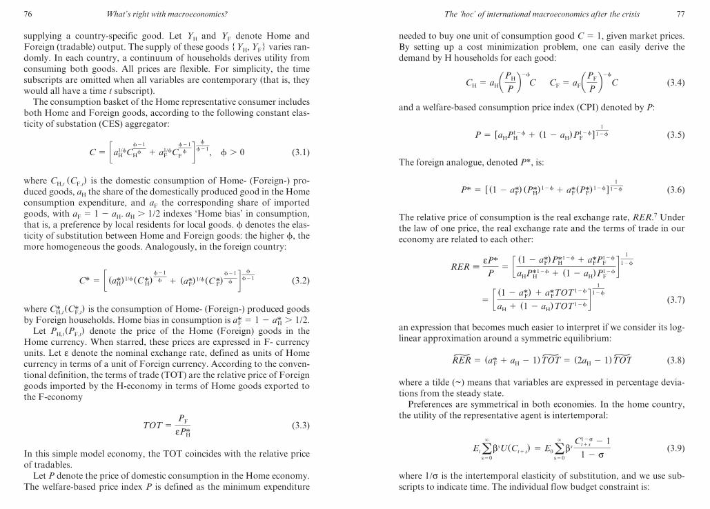
76 What’s right with macroeconomics?
supplying a country- specific good. Let YH and YF denote Home and
Foreign (tradable) output. The supply of these goods {YH, YF} varies ran-
domly. In each country, a continuum of households derives utility from
consuming both goods. All prices are flexible. For simplicity, the time
subscripts are omitted when all variables are contemporary (that is, they
would all have a time t subscript).
The consumption basket of the Home representative consumer includes
both Home and Foreign goods, according to the following constant elas-
ticity of substation (CES) aggregator:
C 5 ca1/�H C
�21
�H 1 a1/�
F C�21
�F d �
�21, � . 0 (3.1)
where CH,t (CF,t
) is the domestic consumption of Home- (Foreign-) pro-
duced goods, aH the share of the domestically produced good in the Home
consumption expenditure, and aF the corresponding share of imported
goods, with aF 5 1 2 aH. aH . 1/2 indexes ‘Home bias’ in consumption,
that is, a preference by local residents for local goods. � denotes the elas-
ticity of substitution between Home and Foreign goods: the higher �, the
more homogeneous the goods. Analogously, in the foreign country:
C* 5 c (a*H)1/� (C*H)�21
� 1 (a*F)1/� (C*F)�21
� d �
�2 1 (3.2)
where C*H,t(C*F,t
) is the consumption of Home- (Foreign- ) produced goods
by Foreign households. Home bias in consumption is a*F 5 1 2 a*H . 1/2.
Let PH,t(PF,t
) denote the price of the Home (Foreign) goods in the
Home currency. When starred, these prices are expressed in F- currency
units. Let e denote the nominal exchange rate, defined as units of Home
currency in terms of a unit of Foreign currency. According to the conven-
tional definition, the terms of trade (TOT) are the relative price of Foreign
goods imported by the H- economy in terms of Home goods exported to
the F- economy
TOT 5PF
eP*H (3.3)
In this simple model economy, the TOT coincides with the relative price
of tradables.
Let P denote the price of domestic consumption in the Home economy.
The welfare- based price index P is defined as the minimum expenditure
M3014 - SOLOW TEXT.indd 76 21/11/2012 13:03
The ‘hoc’ of international macroeconomics after the crisis 77
needed to buy one unit of consumption good C 5 1, given market prices.
By setting up a cost minimization problem, one can easily derive the
demand by H households for each good:
CH 5 aHaPH
Pb2�
C CF 5 aFaPF
Pb2�
C (3.4)
and a welfare- based consumption price index (CPI) denoted by P:
P 5 [aHP12�H 1 (1 2 aH
)P12�F
]1
12� (3.5)
The foreign analogue, denoted P*, is:
P* 5 [ (1 2 a*F) (P*H)12� 1 a*F (P*F)12� ]1
12� (3.6)
The relative price of consumption is the real exchange rate, RER.7 Under
the law of one price, the real exchange rate and the terms of trade in our
economy are related to each other:
RER ;eP*P
5 c (1 2 a*F)P*H12� 1 a*FP12�F
aHP*12�H 1 (1 2 aH
)P12�F
d 1
12�
5 c (1 2 a*F) 1 a*FTOT 12�
aH 1 (1 2 aH)TOT 12�
d 1
12�
(3.7)
an expression that becomes much easier to interpret if we consider its log-
linear approximation around a symmetric equilibrium:
RER|
5 (a*F 1 aH 2 1)TOT|
5 (2aH 2 1)TOT|
(3.8)
where a tilde (~) means that variables are expressed in percentage devia-
tions from the steady state.
Preferences are symmetrical in both economies. In the home country,
the utility of the representative agent is intertemporal:
Eta`
s50
bsU(Ct1s) 5 E0a
`
s50
bsC12s
t1s 2 1
1 2 s (3.9)
where 1/s is the intertemporal elasticity of substitution, and we use sub-
scripts to indicate time. The individual flow budget constraint is:
~ ~ ~
M3014 - SOLOW TEXT.indd 77 21/11/2012 13:03

78 What’s right with macroeconomics?
BH,t11 1 3qH,t(st11
)BH,t11(st11
)dst11 # (1 1 it)BH,t 1 BH,t 1 PH,tYH,t
2 PH,tCH,t 2 PF,tCF,t
where BH,t is the holdings of state- contingent claims priced at qH,t,
paying off one unit of domestic currency in the realized state of the
world as of t, st, and it is the yield on a domestic nominal bond BH,t paid
at the beginning of period t in domestic currency but known at time
t 2 1.
At the aggregate level, the resource constraint is:
YH 5 CH 1 C*H Y*F 5 CF 1 C*F (3.10)
Holding the law of one price, total demand for good H and F can be
written as:
YH 5 aPH,t
Pt
b2�
(aHCt 1 a*HRER�t C*t ) (3.11)
Y*F 5 aPF,t
Pt
b2�
(aFCt 1 RER�t a*FC*t)
Having defined the structure of the model, I can now delve into an
analysis of allocations differing by the structure of the asset market.
Specifically, I will contrast economies with complete markets with econo-
mies only trading a non- contingent bond across borders.
Roots and Consequences of Inefficient (Over) Borrowing and Lending
The market allocation in the case of complete financial markets identifies
the appropriate welfare benchmark against which to define inefficient,
excessive borrowing and lending. In a one- good world, if a complete set
of Arrow–Debreu securities are traded across border (so that households
can invest in as many assets as there are states of the world), marginal
utility growth is equalized across countries in any contingency. Given that
consumption baskets are not realistically identical and that PPP does not
hold, one needs to account for differences in the price of consumption.
By building on this basic theoretical result, David Backus and Gregor
Smith (1993) combine the Euler equations for the Arrow–Debreu Home
and Foreign securities to show that with perfect risk- sharing the ratio of
Home- to- Foreign marginal utility of consumption is tightly linked to the
real exchange rate, namely,
M3014 - SOLOW TEXT.indd 78 21/11/2012 13:03
The ‘hoc’ of international macroeconomics after the crisis 79
RER 5U*CUC
5 a C
C*bs
(3.12)
Taking a log- linear approximation of this expression, again in the
neighbourhood of a symmetric equilibrium with a*F 5 aH, we obtain the
following key condition, characterizing perfect risk- sharing:
s(C| fb 2 C*| fb) 5 RER
| fb (3.13)
where the superscript fb indicates that, in our simple model, prices and
quantities in such allocation are ‘first- best’.
Given the above condition (note that I have included no preference
shocks in the analysis),8 perfect risk- sharing implies that relative consump-
tion and the real exchange rate be perfectly correlated. This is contrary to
some popular but incorrect views, stating that perfect insurance should
produce perfect correlation of consumption across individuals/countries.
As apparent from the model, perfect correlation of consumption only
obtains under the extreme, counterfactual assumption of purchasing
power parity – whereas with identical consumption baskets (aH 5 a*F) , the
real exchange rate is identically equal to 1, and thus invariant to shocks.
In general, with the relative price of consumption changing in response to
shocks, perfect risk- sharing implies that demand should be relatively high
where the price of consumption is relatively low (Gravelle and Rees, 1992)
– that is, in the country whose currency is relatively weak in real terms.
So, suppose that international financial markets are developed enough
to ensure that agents can efficiently share production risk across borders
– for example, suppose all households invest in a well- diversified port-
folio of Home and Foreign equities.9 What happens when, in reaction to a
‘news shock’, agents anticipate higher output in the Home country in the
future? To answer that question, let us inspect the equilibrium relations
between consumption and output on the one hand, and the terms of trade
and output on the other, that can be derived in an economy with perfect
risk- sharing. These are:
(C|fb 2 C*| fb) 5
2aH 2 1
[1 2 (2aH 2 1)2 ]�s 1 (2aH 2 1)2(Y|
Hfb 2 Y
|Ffb) (3.14)
TOT| fb 5
s[1 2 (2aH 2 1)2 ]�s 1 (2aH 2 1)2
(Y|
Hfb 2 Y
|Ffb) (3.15)
Observe first that the coefficients on the right- hand side of both
equations are positive. With perfect risk- sharing, Home consumption
~~
~
~
M3014 - SOLOW TEXT.indd 79 21/11/2012 13:03

80 What’s right with macroeconomics?
necessarily rises relative to Foreign consumption, and the Home terms of
trade necessarily deteriorate in response to an increase in Home relative to
Foreign output.
Most crucially, however, observe also that all the variables in the above
expressions are contemporaneous. This is a key property of the complete
market allocation in the above model: current relative consumption and
current relative prices (both the terms of trade and the real exchange rates)
do not depend at all on expectations of future output. In response to ‘news
shocks’, there is no change in these variables. The reason is straightfor-
ward. Namely, if global portfolios are well diversified, the anticipation
of future high profits in a region raises wealth everywhere in the world
economy. In relative terms, there would be no demand imbalance. Minus
supply reactions in the short run (the ‘news’ is about future, not current
output), there is no need for a change in the terms of trade and the real
exchange rate. The only variable that must react to the news is the inter-
est rate, rt, as the Euler equations in the asset markets imply that the
current price of default- free bonds adjusts in anticipation of higher future
consumption:
1
1 1 rt
5 bEt cUC(Ct11
)
UC(Ct
)d (3.16)
Intuitively, in equilibrium, the real rate must rebalance world demand
towards future periods when production is expected to be more abundant
– that is, the intertemporal price of consumption must change to lead
households to postpone (optimally) their spending plan.
Now, let us contrast the market equilibrium with the perfect markets
just analysed, with the equilibrium in economies where portfolios are not
well diversified and markets are incomplete. To make the main point of
the analysis as clear as possible, assume that preferences are logarithmic,
and the pure rate of time preference is zero (that is, s 5 b 5 1). Moreover,
agents can trade internationally a non- contingent bond only – that is, they
can borrow and lend cross border, but cannot write insurance contracts
(see also Corsetti et al., 2008). Furthermore, for notational simplicity,
time is collapsed into two periods, the ‘present’ and the ‘future’, dubbed
the short- run (SR) and the long- run (LR). Under these assumptions and
notational convention, it can be shown that both relative consumption
and the terms of trade move with both current and anticipated future
output as follows:
(C|SR 2 C
|*SR) 5 (2aH 2 1) c (Y
|SRH 2 Y
|LRH
) 2 (Y|SR
F 2 Y|LR
F)
1 2 4aH(1 2 aH
) (1 2 �)
~~ ~ ~ ~
~
M3014 - SOLOW TEXT.indd 80 21/11/2012 13:03
The ‘hoc’ of international macroeconomics after the crisis 81
1 a1 12aH
(� 2 1)
2aH 2 1b Y
|LRH 2 Y
|LRF
1 2 2aH(1 2 �)
d TOT
| SR 5(Y|SR
H 2 Y|LR
H) 2 (Y
|SRF 2 Y
|LRF
)
1 2 4aH(1 2 aH
) (1 2 �)1
Y|LR
H 2 Y|LR
F
1 2 2aH(1 2 �)
(3.17)
Current variables now respond to both current and future anticipated
movements in relative output. With news shocks only, Y|SR
H 5 Y|SR
F 5 0, the
above expressions become:
(C|SR 2 C
|*SE) 5 c [2aH 2 1]
[1 2 2aH(1 2 �) ]
a1 12aH
(� 2 1)
2aH 2 1b
22aH 2 1
[1 2 4aH(1 2 aH
) (1 2 �) ]d (Y|LR
H 2 Y|LR
F)
TOT|
5 c 1
1 2 2aH(1 2 �)
21
1 2 4aH(1 2 aH
) (1 2 �)d (Y|LR
H 2 Y|LR
F)
(3.18)
Only in a special case, when the trade elasticity happens to be one
(� 5 1), do the coefficients in front of relative output become zero in both
expressions (3.18).10 As is well known (see Cole and Obstfeld, 1991), under
this restriction on the parameters’ values, the allocation with and without
financial markets coincide by virtue of the automatic insurance provided
by terms of trade movements.11 In general, however, and different from
the case of complete markets above, news shocks will have contemporane-
ous effects on the market allocation and induce exchange rate volatility.
When markets are incomplete, news shocks stretch, so to speak, the
dual role of the exchange rate as equilibrium price in the goods and the
assets market. The exchange rate jumps upon the arrival of information
about future output and moves so as to clear the goods market in response
to an increase in domestic demand. Indeed, with home bias (aH . 1/2),
both a high trade elasticity (� sufficiently above 1) or a low trade elasticity
(� sufficiently below 1) imply that the coefficient in front of future (Home
to Foreign) relative output is positive in the relative- consumption expres-
sion (3.18), while negative in the terms of trade expression. This means
that Home consumption expands, and the Home terms of trade (and real
exchange rate) strengthen, in response to anticipations of a larger Home
output in the future. Observe that in a low elasticity environment, the two
coefficients relating relative output to relative consumption and the terms
of trade can become quite large. For any given news shock, there will be
~ ~
~
~ ~
~~~~ ~
~ ~
~
~
~ ~
~~
M3014 - SOLOW TEXT.indd 81 21/11/2012 13:03

82 What’s right with macroeconomics?
much larger effects on relative demand, a larger current account, and a
larger real appreciation, relative to economies characterized by a high
trade elasticity.
The transmission mechanism just described is a textbook example of
optimal consumption smoothing. Anticipations of output gains in the
Home country necessarily translate into an asymmetric wealth shock in
favour of Home residents. Since they have access to the international
bonds market, Home agents are able to raise their current consumption by
borrowing abroad, generating an external trade deficit. To the extent that
the composition of national demand is biased towards domestic goods
(which is indeed the case, especially in relatively large economies such
as the US), higher demand results in higher prices, that is, real currency
appreciation in the short run.
The equilibrium just described is also familiar from the vantage point of
conventional models in the Mundell–Fleming tradition (see, for example,
Marston, 1985). In this framework, real appreciation in response to (exog-
enous) demand movements is typically seen as a channel through which
the domestic economy is naturally ‘stabilized’. If domestic demand rises in
anticipation of future income, the real appreciation is expected to counter-
act domestic ‘over- heating’ by ‘crowding-out net exports’.12
Relative to these conventional considerations, nonetheless, the simple
algebra above makes it clear that appreciation and external deficits are
in fact highly inefficient. In a well- functioning market economy in which
agents hold well- diversified portfolios, the country expected to produce
more output (that is, with more productive firms) would not become a
net importer to sustain a consumption demand boom. Over time, when
output increases, if anything it will experience falling, rather than rising,
product prices.
In more general model specifications with capital accumulation, of
course, a trade deficit may emerge also in efficient economies in response
to expectations of future gains in productivity (this would be so, for
instance, in the presence of a sufficiently tight ‘time- to- build’ techno-
logical constraint on capital accumulation). But trade deficits in this case
would be driven by the expansion of investment into efficient capital, not
by inefficient movements in cross- country consumption. In other words,
what is at stake is not the desirability of trade deficits/surpluses per se,
but excessive borrowing and lending as an undesirable consequence of
economic distortions.
It may be worth stressing, for instance, that intertemporal trade in a
distorted economy provides no safeguard/insurance against the possibil-
ity that the anticipations of future output gains produced by the news
shock turn out to be wrong ex post (that is, that the higher output does
M3014 - SOLOW TEXT.indd 82 21/11/2012 13:03
The ‘hoc’ of international macroeconomics after the crisis 83
not materialize in the future). Let us focus again on our model economy
without capital. With international borrowing and lending through trade
in bonds, wrong expectations today create the premise for costly adjust-
ment in the future – the Home country ends up with the cost of servicing
additional foreign debt without the benefit of a higher output. In contrast,
with efficient portfolio diversification ensuring perfect risk- sharing, news
shocks produce no change in relative consumption in the short run, no
external deficit, hence no need for costly adjustment in the future.13 Also
in this dimension, the main message is that the financial distortions of
intertemporal trade may exacerbate inefficiencies.
In general, the full extent of the distortions can be assessed by solving
for the constrained Pareto- efficient allocation in an economy with incom-
plete markets.14 The solution will generally prescribe agents to react much
less to anticipations of future output gains relative to the market alloca-
tion. Namely, the social planner will mandate agents to react only to the
changes in output (now and expected in the future), which are efficient
from a global perspective – not to output movements that depart from the
first- best allocation (see Corsetti et al., 2010b).
RETHINKING POLICY MODELS
The model discussed in the previous section is admittedly too simple to get
into the nuances of policy design. Yet the analysis conveys a key message
underlying much of the recent work on stabilization policy, carried out in
the framework of large macro models. The model economy characterized
above, in particular, illustrates the core theoretical foundations of cross-
border imbalances and misalignment in the context of micro- founded
models for policy assessment, as discussed in detail in the joint work by
Corsetti, Dedola and Leduc (2010a, 2010b) describing optimal monetary
policy in an open economy. In addition to the output gap as defined in
standard (new- Keynesian) monetary theory, a model of global stabiliza-
tion naturally includes gaps in international relative prices, and a gap in
international demand.
Relative price gaps identify a theory- based measure of misalignment,
encompassing the real exchange rate (the relative price of consumption),
the terms of trade (the relative price of imports in terms of exports), as
well as differences in prices of similar products across borders (that is,
failure of the law of one price). By way of example, the terms of trade
gap are defined as the log- difference between the values of the terms of
trade in the distorted market allocation and in the efficient (first- best)
allocation:
M3014 - SOLOW TEXT.indd 83 21/11/2012 13:03

84 What’s right with macroeconomics?
TOTgap 5 logTOT
TOTfb (3.19)
It is worth stressing that inefficiencies in international relative prices
reflect more than nominal rigidities. As the stylized economy in the previ-
ous section clarifies, for flexible prices as well, the terms of trade (and the
real exchange rate) are generally inefficient if markets are not perfect.
Note that the relevant misalignment captured by the relative price gap
does not necessarily coincide with deviations from the ‘equilibrium real
exchange rate’ typically studied by international organizations in rela-
tion to long- term objectives of ‘external and internal balances’. Rather,
the price gap is defined conceptually and analytically like the output gap,
over short as well as long horizons. Like the output gap, it is difficult to
estimate in practice.
By the same token, the relative demand gap provides a theory- based
measure of cross- border imbalances:
Dgap 5 log cRERUC
U*Cd 5 log cRERa C
C*b2 s d (3.20)
The so- defined gap is equal to zero when risk- sharing is perfect. A
non- zero value instead points to situations in which, at the current real
exchange rate, consumption in one country is inefficiently high relative to
consumption in the rest of the world, which evolves into inefficient current
account deficits and capital inflows, as well as into general misallocation
of production at domestic and international levels.
These gaps are relevant to policy making, in the same way that output
gaps and inflation are. The welfare- based objective function for the analy-
sis of optimal policy can (and should) in fact be written as a function of
all these gaps. In addition to the adverse consequences of nominal price
frictions, it is natural for policy makers to confront the consequences
of financial frictions (incomplete markets), causing over- borrowing,
inefficient movements in international relative prices, as well as sub-
optimal employment and consumption levels, relative to the efficient
allocation benchmark. Given the set of the available policy instruments,
stabilization policy needs to be optimized over the trade- offs among the
competing objectives, meaning, closing all the welfare- relevant gaps.
Some striking results concern monetary policy. Corsetti et al. (2010a,
2010b) show that in more general versions of the incomplete market
economy above (accounting for an elastic labour supply, production and
sticky prices), there are reasonable parameter configurations for which
monetary policy is particularly effective in preventing both mispric-
M3014 - SOLOW TEXT.indd 84 21/11/2012 13:03
The ‘hoc’ of international macroeconomics after the crisis 85
ing (inefficient appreciation) and over- borrowing (global imbalances in
demand). Specifically, under international policy coordination, monetary
authorities optimally ‘lean against the wind’ of appreciation and external
imbalances, improving the world allocation at small costs in terms of
short- run domestic inflation: price stability remains the overriding objec-
tive in the medium run. Importantly, the optimal conduct of monetary
policy does not imply unreasonable variations in interest rates. Indeed,
in their calculations, the variance of the interest rate is quite contained,
relative to a suboptimal regime of inflation targeting that ignores these
important dimensions of the optimal monetary policy.
The degree to which monetary policy is effective as a stabilization tool
varies across economies with different structures. Under some parameter-
izations of the model, monetary instruments are optimally geared mostly
towards closing output gaps and keeping prices stable – the traditional,
inward- looking objectives. But even so, there are other tools available to
policy makers to address potential concerns. When monetary policy is
ineffective, or to the extent that its use is deemed inappropriate relative
to the task of correcting excessive borrowing and misalignments, alterna-
tive instruments may and should be considered, ranging from fiscal policy
(raising issues in fiscal and monetary interactions), to regulation and
supervision of financial markets.
The recent evolution in the literature on open economies provides a
clear example of the ongoing shift in theory and policy analysis, catalysed
by the global crisis. Before the crisis, most of the discussion was framed in
models predicting a high degree of equilibrium risk- sharing, thus centring
the analysis almost exclusively on the distortions due to nominal rigidities
(see, for example, the discussion in Corsetti, 2008). Also in this context,
misalignments in international pricing and consumption demand are pos-
sible, but these exist only as a by- product of sticky prices – for instance,
with complete markets, the demand gap (3.20) is always identically equal
to zero. Once nominal distortions are redressed, the economy operates
near first- best. Indeed, in this context, it is easy to produce examples of the
‘divine coincidence’ discussed by Olivier Blanchard and Jordi Galí (2010),
whereas one instrument is enough to close all the relevant gaps in the
economy. Heterogeneity across borders appears to raise no specific policy
issues – see, for example, the conclusions from the collection of essays in
Jordi Galí and Mark Gertler (2009) on the ‘International dimensions of
monetary policy’. The new contributions in international economics are
clearly moving away from this premise.
More contributions need to be written in this area of economics. By
way of example, the analysis above assumes that asset prices – namely, the
exchange rate – react to fundamentals only. Indeed, in the model, the real
M3014 - SOLOW TEXT.indd 85 21/11/2012 13:03

86 What’s right with macroeconomics?
exchange rate moves only in reaction to new information about current
and future fundamentals – it acts as a ‘shock absorber’. Yet, its adjustment
is inefficient because of the distortions plaguing the market economy. An
important new avenue of research could provide workable frameworks
where asset prices are driven by bubbles, identifying plausible conditions
for these to arise, and especially clarifying the scope for addressing them
via alternative policy strategies.
While the economic example used in this text draws on international
economics, my own field of specialization, it should be clear that similar
analytical schemes could be developed to understand income and produc-
tion dynamics, accounting for sectoral or regional differences, or hetero-
geneity in wealth and/or participation in financial markets across agents
within the same national economy, sharing the same currency. Also in
these contexts, inefficient markets would, in general, be associated with
demand imbalances (excessive borrowing) among heterogeneous agents
and misalignments in relative prices – although exchange rate movements,
in their unique function of clearing both the goods and the asset markets,
would obviously be out of the picture.
NOTES
1. I thank Charles Gottlieb and Saverio Simonelli for comments.
2. On account of the crisis, there is a long list of excellent contributions. The chapter relies
mostly on my own experience (working in the European Economic Advisory Group at
CESifo, 2009), as well as on the contributions of Markus Brunnermeier (2009), Gary
Gorton (2009), and John Taylor (2009), among others.
3. See http://www.nyu.edu/econ/user/gertlerm/gertlerboereadinglist.pdf.
4. Lawrence Peter ‘Yogi’ Berra (born 12 May, 1925) is not only widely regarded as one
of the greatest catchers in baseball history: his legendary quotations provide an endless
source of wit and wisdom in graduate schools in economics and other disciplines in the
USA.
5. A very incomplete list includes Bianchi and Mendoza (2010), Brunnermeier and
Sannikov (2011), Curdia and Woodford (2010), Geanakoplos (2010b) and Lorenzoni
(2009), among many others.
6. In addition to the list above, see also Bianchi (2011), Christiano et al. (2009),
Geanakoplos (2010a), Gertler and Kiyotaki (2010).
7. Note that if the law of one price holds in the goods markets, once converted into a
common currency, the price of each good will be identical everywhere in the world
economy: PH 5 eP*H, PF 5 eP*F. Then, if the Home and Foreign consumption baskets
were identical, namely, if there was no Home bias in the world economy, aH 5 1 2 a*F,
the price of consumption would also be equalized across countries and purchasing
power parity (PPP) would hold: P 5 eP*. In what follows, home bias will be assumed
throughout the analysis.
8. With taste shocks, the strict link between the relative marginal utilities and the relative
price of consumption in (3.12), implied by perfect risk- sharing, would not necessarily
translate into a strict link between quantities and prices (as in (3.13)).
9. When production/output uncertainty is the most important source of risk (that is,
M3014 - SOLOW TEXT.indd 86 21/11/2012 13:03
The ‘hoc’ of international macroeconomics after the crisis 87
shocks to tastes are absent or small enough), it can be shown that the perfect risk-
sharing condition above would hold approximately, even if there were not as many
financial markets as states of the world. Agents in each country could nevertheless
invest in a well diversified portfolio of domestic and foreign stocks, so as to share
income generated by firms everywhere in the world. In other words, perfect diversifica-
tion of equity would be enough to guarantee full insurance against production risk.
10. See Corsetti et al. (2010a) for a discussion of more general conditions in the log-
linearized version of the model.
11. With unit elasticity, any increase in Home output is matched by a proportional fall
in the international price of domestic goods, raising the purchasing power of foreign
residents in line with that of domestic residents. Relative (Home to Foreign) incomes
remain in fixed ratio.
12. But this reasoning downplays the first- order implications of the boost in Home private
wealth and demand from favourable movements of the terms of trade in the short run –
in our example, it is inherently connected to the ability of agents to borrow from abroad
against future income. Indeed, the structure of traditional models fails to account for
the fact that real appreciation also has a positive feedback effect on the asymmetric
wealth effects from shocks, feeding external imbalances.
13. Of course, with capital accumulation, time- to- build or adjustment cost in investment
may mean that investment reacts immediately to the news shock. This may also create
costly adjustment over time if the anticipation of higher future productivity turns out
to be wrong.
14. Specifically, this is the solution to the problem of the social planner, maximizing a
weighted sum of the expected utilities of the Home and Foreign residents, subject to
the same informational and institutional constraints faced by agents in the incomplete
market economy.
REFERENCES
Aoki, K., G. Benigno and N. Kiyotaki (2009a), ‘Adjusting to capital account lib-eralization’, mimeo, Princeton University.
Aoki, K., G. Benigno and N. Kiyotaki (2009b), ‘Capital flows and asset prices’, mimeo, Princeton University.
Backus, D.K. and G.W. Smith (1993), ‘Consumption and real exchange rates in dynamic economies with non- traded goods’, Journal of International Economics, 35, 297–316.
Bianchi, J. (2011), ‘Overborrowing and systemic externalities in the business cycle’, American Economic Review, 101(7), 3400–426.
Bianchi, J. and E. Mendoza (2010), ‘Overborrowing, financial crises and macro- prudential policy’, NBER Working Paper 16091.
Blanchard, O. and J. Galí (2010), ‘Labor market frictions and monetary policy: a new Keynesian model with unemployment’, American Economic Journal: Macroeconomics, 2(2), 1–30.
Bloom, N. (2009), ‘The impact of uncertainty shocks’, Econometrica, 77(3), 623–85.Bolton, P. and O. Jeanne (2011), ‘Sovereign default risk and bank fragility in
financially integrated economies’, NBER Working Paper 1689.Brunnermeier, M. (2009), ‘Deciphering the liquidity and credit crunch 2007–08’,
Journal of Economic Perspectives, 23(1), 77–100.Brunnermeier, M. and Y. Sannikov (2011), ‘A macroeconomic model with a finan-
cial sector’, mimeo, Princeton University.
M3014 - SOLOW TEXT.indd 87 21/11/2012 13:03

88 What’s right with macroeconomics?
Caballero, R. (2010), ‘A caricature (model) of the world economy’, paper prepared for the Ninth Macroeconomic Policy Research Workshop, ‘Understanding financial frictions’, Magyar Nemzeti Bank, Budapest.
Caballero, R., E. Farhi and P.O. Gourinchas (2008), ‘Financial crash, commodity prices, and global imbalances’, Brookings Papers on Economic Activity, Fall, pp. 1–55.
Christiano, L., R. Motto and M. Rostagno (2009), ‘Financial factors in economic fluctuations’, mimeo, Northwestern University.
Cole, H.L. and M. Obstfeld (1991), ‘Commodity trade and international risk sharing: how much do financial markets matter?’, Journal of Monetary Economics, 28, 3–24.
Corsetti, G. (2008), ‘New open economy macroeconomics’, in Steven N. Durlauf and Lawrence E. Blume (eds), The New Palgrave Dictionary of Economics, 2nd edn, Basingstoke: Palgrave Macmillan.
Corsetti, G., L. Dedola and S. Leduc (2008), ‘International risk sharing and the transmission of productivity shocks’, Review of Economic Studies, 75, 443–73.
Corsetti, G., L. Dedola and S. Leduc (2010a), ‘Optimal monetary policy in open economies’, in B.M. Friedman and M. Woodford (eds), Handbook of Monetary Economics, vol. 3, Amsterdam: Elsevier, pp. 861–933.
Corsetti, G., L. Dedola and S. Leduc (2010b), ‘Demand imbalances, exchange rates misalignment and monetary policy’, mimeo, Cambridge University.
Curdia, V. and M. Woodford (2010), ‘Credit spreads and monetary policy’, Journal of Money Credit and Banking, 42(S1), 3–35.
Eichenbaum, M. (2010), ‘Shortcomings in macro modeling strategies: what have we learned from the crisis?’, paper presented at the Sixth ECB Central Banking Conference, ‘Approaches to monetary policy revisited – lessons from the crisis’, Frankfurt- am- Main, 18–19 November.
European Economic Advisory Group at CESifo (2009), ‘Report on the European economy’, Munich: CESifo.
Fernández- Villaverde, J., P. Guerrón- Quintana, J. Rubio- Ramírez and M. Uribe (2011), ‘Risk matters: the real effects of volatility shocks’, American Economic Review, 101(6), 2530–61.
Galí, J. and M. Gertler (eds) (2009), International Dimension of Monetary Policy, London: The University of Chicago Press.
Geanakoplos, J. (2010a), ‘Solving the present crisis and managing the leverage cycle’, Federal Reserve Bank of New York Economic Policy Review, August, pp. 101–31.
Geanakoplos, J. (2010b), ‘The leverage cycle’, in D. Acemoglu, K. Rogoff and M. Woodford (eds), NBER Macroeconomics Annual 2009, vol. 24, Chicago: University of Chicago Press, pp. 1–65.
Gertler, M. and N. Kiyotaki (2010), ‘Financial intermediation and credit policy in business cycle analysis’, in B.M. Friedman and M. Woodford (eds), Handbook of Monetary Economics, vol. 3, Amsterdam: Elsevier, pp. 547–99.
Gorton, G. (2009), ‘The panic of 2007’, in Maintaining Stability in a Changing Financial System, Proceedings of the 2008 Jackson Hole Conference, Federal Reserve Bank of Kansas City.
Gravelle, H. and R. Rees (1992), Microeconomics, London: Longman.Greenlaw, D., J. Hatzius, A. Kashyap and H.S. Shin (2008), ‘Leveraged losses:
lessons from the mortgage market meltdown’, US Monetary Policy Forum Report no. 2.
M3014 - SOLOW TEXT.indd 88 21/11/2012 13:03
The ‘hoc’ of international macroeconomics after the crisis 89
Gruss, B. and K. Mertens (2010), ‘Regime switching interest rates and fluctuations in emerging markets’, mimeo, Cornell University.
Lorenzoni, G. (2009), ‘A theory of demand shocks’, American Economic Review, 99(5), 2050–84.
Marston, R. (1985), ‘Stabilization policies in open economies’, in R.W. Jones and P.B. Kenen (eds), Handbook of International Economics, Amsterdam: North Holland, pp. 859–916.
Martin, A. and J. Ventura (2011), ‘Theoretical notes on bubbles and the current crisis’, IMF Economic Review, 59, 6–40.
Obstfeld, M. and K. Rogoff (2010), ‘Global imbalances and the financial crisis: products of common causes’, CEPR Discussion Paper 7606.
Reinhart, C. and K. Rogoff (2009), This Time is Different: Eight Centuries of Financial Folly, Princeton, NJ: Princeton University Press.
Shiller, R.J. (2008), The Subprime Solution: How Today’s Global Financial Crisis Happened, and What to Do About it, Princeton, NJ: Princeton University Press.
Taylor, J. (2009), Getting Off Track: How Government Actions and Interventions Caused, Prolonged, and Worsened the Financial Crisis, Stanford, CA: Hoover Institution Press.
Woodford, M. (2010), ‘Financial intermediation and macroeconomic analysis’, Journal of Economic Perspectives, 24(4), 21–44.
M3014 - SOLOW TEXT.indd 89 21/11/2012 13:03

90
4. Try again, macroeconomists
Jean- Bernard Chatelain
INTRODUCTION
The world financial and economic crisis that broke out in the summer of
2007 has sparked ground- breaking thinking in the field of macroeconom-
ics and finance. The purpose of this chapter is to assess where most macro-
economists are in relation to those ideas.
I will begin with a description of the conditions that led to a great
reversal of weakly regulated international finance to strongly regulated
international finance for the period 1945–73. These days the bargain-
ing power of international banking is too strong to observe the same
kind of trend. Weakly regulated international capital markets are likely
to persist in the next decades. There is thus a high probability that
the financial crisis will lead to very costly world recessions in terms of
welfare. For that reason, macroeconomic theory must deal with weakly
regulated international capital markets, which lead to a systematically
erroneous valuation of assets (the efficient market hypothesis is not
valid).
The second section deals with the best theoretical models that were
available before the crisis began in 2007 for dealing with imperfect capital
markets: the ‘financial accelerator’ dynamic stochastic general equilib-
rium (DSGE) models (Kiyotaki and Moore, 1997; Bernanke et al., 1999;
Bernanke and Gertler, 2000, 2001; Iacoviello, 2005). These models consid-
ered bankruptcy costs and credit rationing for non- financial firms and, for
some of them, banking firms. They assumed that debt was backed by the
future valuation of collateral. They maintained the assumption, however,
that the expected valuation of collateral was made according to its fun-
damental value. In other words, they assumed imperfect capital markets
along with the efficient financial market hypothesis. I will list seven
inconsistencies of these models with respect to their ability to describe the
economic crisis.
The third section emphasizes that five key assumptions must be changed
in order to change mainstream macroeconomics: (1) the absence of a
M3014 - SOLOW TEXT.indd 90 21/11/2012 13:03
Try again, macroeconomists 91
confidence crisis or liquidity crisis with systemic bankruptcy risk; (2) the
efficient financial market hypothesis where the price of an asset is always
equal to its fundamental value; (3) the no- Ponzi Game condition, such
that the growth rate of public and private debt must always be below a
real interest rate; (4) the linearization around the equilibrium of the unique
stable path leading to a unique long- term equilibrium, reducing the study
of macroeconomic dynamics to qualitatively similar responses of mac-
roeconomic variables to shocks; (5) the unconstrained Euler equation
for households, where the growth rate of consumption depends only on
the real interest rate and on the preference for smoothing consumption
over time. These assumptions are compatible with the structural research
programme that takes into account the Lucas critique (1976). I will then
briefly sketch that the ongoing macroeconomics research may come close
to our goal, but haltingly.
IT CAN HAPPEN AGAIN TOMORROW
A Great Reversal in the Regulation of International Finance?
What is expected to change in the real economy in the two decades follow-
ing the crisis? Let us consider two possibilities with the following stylized
facts describing two regulation regimes.
1. Weakly regulated international finance (regime A): international
banking capital flows and offshore finance lead to widespread
opacity.
● A1. International banks that trade international assets have
balance sheets that are highly uncertain (on their solvency).
They may use offshore financing to hide profits (tax evasion)
and losses (soft budget constraint).
● A2. The share of assets, whose valuation is highly uncertain and
never close to the fundamental value, is large.
● A3. Incentives are there for banks to take huge risks due to
the bail- out by the government of banks that are too intercon-
nected. Banks therefore remain highly leveraged in a weakly
regulated financial system.
● A1, A2 and A3 lead to a larger probability of an expectation-
driven, loss- of- confidence systemic crisis, in particular among
banks, which are more aware of the risk of other banks than
depositors. This could be expected to occur, say, once every
three normal business cycles of eight years.
M3014 - SOLOW TEXT.indd 91 21/11/2012 13:03

92 What’s right with macroeconomics?
● Universal banks doing retail banking and market finance opera-
tions are likely to increase the risk of the transmission of bubbles
on asset prices to the real economy through credit. Capital gains
and losses on the equity market would be linked to simultane-
ous increases or (respectively) decreases in retail credit.
● In this context, government- owned banks able to do interna-
tional finance are likely to speculate in the same way as pri-
vately owned banks, because it has become too easy to make
profits and losses in the same manner as their privately owned
competitors.
The benefit of this regime is a potentially better allocation of capital
at the international level, along with the drawback of a higher
probability of systemic risk at the world level.
2. Strongly regulated international finance (regime B) is an alternative
regime. It implies the control of the international capital flows of
large international banks, and the control of the amount of credit by
large retail banks in order to limit bubbles at the national level, when
this amount of credit is ‘too high’ or ‘too low’ for small and medium-
sized firms or households (strong macro- prudential policy). This
means that the government is highly involved in the decisions on the
allocation of capital.
The drawback of the strong regulation regime B may be a mis-
allocation of capital at the international level; its advantage is a lower
probability of systemic risk at the world level.
The shift from regime A to regime B is a ‘great reversal’ as
described by Raghuram Rajan and Luigi Zingales (2003), similar to
the one that followed the Bretton Woods United Nations Monetary
and Financial Conference from 1945–73, with respect to the period
1870–1940.
The Weak Bargaining Power of International Banking in 1945
Let us consider an incomplete list of the conditions under which regime B
occurred after 1945, leading to a great reversal:
● immediate post- war economy with a strong government stake in the
allocation of capital;
● future reconstruction plans with a strong government stake in the
allocation of capital (Marshall Plan Aid), along with competition
with the Soviet Union’s economic system;
● capitalism in search of employment stability for wage earners, with
a weaker influence of the owners of capital;
M3014 - SOLOW TEXT.indd 92 21/11/2012 13:03
Try again, macroeconomists 93
● international banking in shambles in several countries due to war
and destruction;
● weak political pressure to ensure stability of exchange rates.
The Bretton Woods context occurred simultaneously with other factors
that supported a great reversal in the relative bargaining power of
international banking and finance:
● international capital flows decreased and were under the control of
the government;
● international trade decreased widely;
● government stakes in the banking sector in the allocation of capital
remained large in a number of countries (France, Japan, Germany);
● large stakes of the private banking sector were confined to national
retail banking, while facing: effective direct credit control in France
up to 1983, competition of nationalized financial institutions for
deposits (Japanese post office), and regulatory walls against cross-
state banking in the USA and against universal banking (merging
retail banking with market- finance activities banking), with the
Glass–Steagall Act enacted in 1933 (a law that established the
Federal Deposit Insurance Corporation in the United States and
introduced banking reforms).
The Bretton Woods agreements led to a large decrease in the world
occurrence of financial crises for the period 1945–73, as recorded by
Carmen Reinhart and Kenneth Rogoff (2009). This is a key explanation of
the low frequency of world financial crises over the last 100 years. Hence,
any computation of the probability of the occurrence of a world finan-
cial crisis has to deal with the relative bargaining power of international
finance with respect to governments and wage earners, in particular in its
ability to limit the control of international capital flows and maintain a
large degree of opacity on those international capital flows.
The Strong Bargaining Power of International Banking in 2010
In 2010, the pre- conditions of the Bretton Woods era, which were already
limiting the bargaining power of international banking, were obviously
not met. The current economic and geopolitical framework is completely
different from the immediate post- World-War-Two context of Bretton
Woods in 1945. Unless, perhaps, several very large countries of the G7
default on their sovereign debt, which would leave the door open to unin-
tended consequences, the balance of power between international finance,
M3014 - SOLOW TEXT.indd 93 21/11/2012 13:03
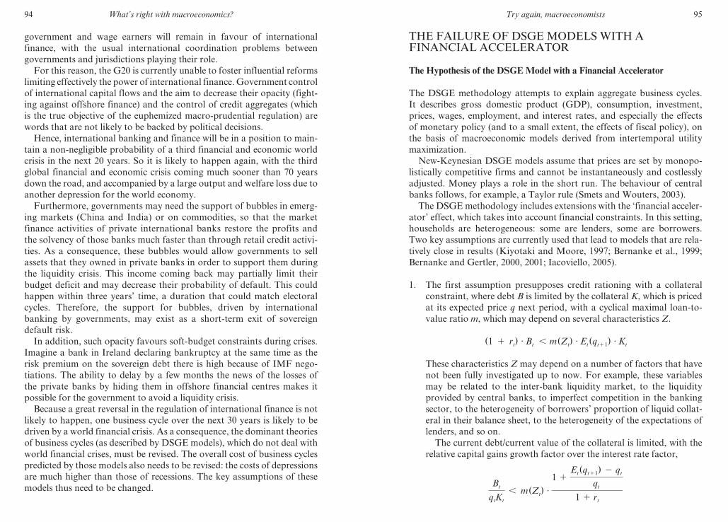
94 What’s right with macroeconomics?
government and wage earners will remain in favour of international
finance, with the usual international coordination problems between
governments and jurisdictions playing their role.
For this reason, the G20 is currently unable to foster influential reforms
limiting effectively the power of international finance. Government control
of international capital flows and the aim to decrease their opacity (fight-
ing against offshore finance) and the control of credit aggregates (which
is the true objective of the euphemized macro- prudential regulation) are
words that are not likely to be backed by political decisions.
Hence, international banking and finance will be in a position to main-
tain a non- negligible probability of a third financial and economic world
crisis in the next 20 years. So it is likely to happen again, with the third
global financial and economic crisis coming much sooner than 70 years
down the road, and accompanied by a large output and welfare loss due to
another depression for the world economy.
Furthermore, governments may need the support of bubbles in emerg-
ing markets (China and India) or on commodities, so that the market
finance activities of private international banks restore the profits and
the solvency of those banks much faster than through retail credit activi-
ties. As a consequence, these bubbles would allow governments to sell
assets that they owned in private banks in order to support them during
the liquidity crisis. This income coming back may partially limit their
budget deficit and may decrease their probability of default. This could
happen within three years’ time, a duration that could match electoral
cycles. Therefore, the support for bubbles, driven by international
banking by governments, may exist as a short- term exit of sovereign
default risk.
In addition, such opacity favours soft- budget constraints during crises.
Imagine a bank in Ireland declaring bankruptcy at the same time as the
risk premium on the sovereign debt there is high because of IMF nego-
tiations. The ability to delay by a few months the news of the losses of
the private banks by hiding them in offshore financial centres makes it
possible for the government to avoid a liquidity crisis.
Because a great reversal in the regulation of international finance is not
likely to happen, one business cycle over the next 30 years is likely to be
driven by a world financial crisis. As a consequence, the dominant theories
of business cycles (as described by DSGE models), which do not deal with
world financial crises, must be revised. The overall cost of business cycles
predicted by those models also needs to be revised: the costs of depressions
are much higher than those of recessions. The key assumptions of these
models thus need to be changed.
M3014 - SOLOW TEXT.indd 94 21/11/2012 13:03
Try again, macroeconomists 95
THE FAILURE OF DSGE MODELS WITH A FINANCIAL ACCELERATOR
The Hypothesis of the DSGE Model with a Financial Accelerator
The DSGE methodology attempts to explain aggregate business cycles.
It describes gross domestic product (GDP), consumption, investment,
prices, wages, employment, and interest rates, and especially the effects
of monetary policy (and to a small extent, the effects of fiscal policy), on
the basis of macroeconomic models derived from intertemporal utility
maximization.
New-Keynesian DSGE models assume that prices are set by monopo-
listically competitive firms and cannot be instantaneously and costlessly
adjusted. Money plays a role in the short run. The behaviour of central
banks follows, for example, a Taylor rule (Smets and Wouters, 2003).
The DSGE methodology includes extensions with the ‘financial acceler-
ator’ effect, which takes into account financial constraints. In this setting,
households are heterogeneous: some are lenders, some are borrowers.
Two key assumptions are currently used that lead to models that are rela-
tively close in results (Kiyotaki and Moore, 1997; Bernanke et al., 1999;
Bernanke and Gertler, 2000, 2001; Iacoviello, 2005).
1. The first assumption presupposes credit rationing with a collateral
constraint, where debt B is limited by the collateral K, which is priced
at its expected price q next period, with a cyclical maximal loan- to-
value ratio m, which may depend on several characteristics Z.
(1 1 rt) # Bt , m(Zt
) # Et(qt11
) # Kt
These characteristics Z may depend on a number of factors that have
not been fully investigated up to now. For example, these variables
may be related to the inter- bank liquidity market, to the liquidity
provided by central banks, to imperfect competition in the banking
sector, to the heterogeneity of borrowers’ proportion of liquid collat-
eral in their balance sheet, to the heterogeneity of the expectations of
lenders, and so on.
The current debt/current value of the collateral is limited, with the
relative capital gains growth factor over the interest rate factor,
Bt
qtKt
, m(Zt) #
1 1Et
(qt11) 2 qt
qt
1 1 rt
M3014 - SOLOW TEXT.indd 95 21/11/2012 13:03
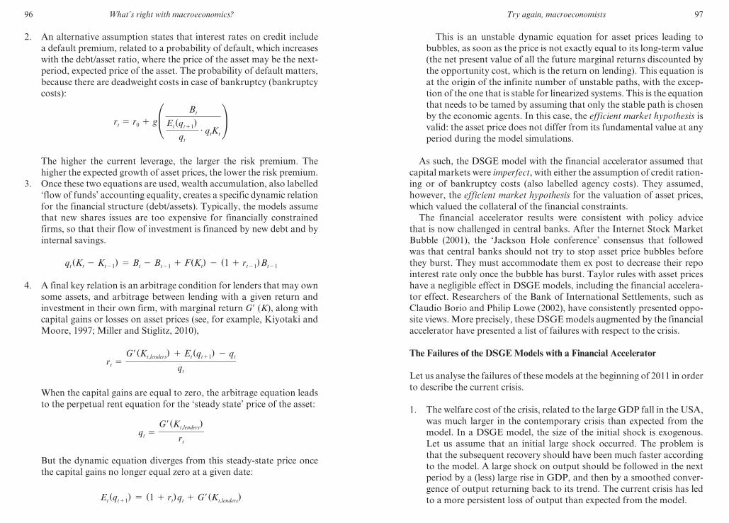
96 What’s right with macroeconomics?
2. An alternative assumption states that interest rates on credit include
a default premium, related to a probability of default, which increases
with the debt/asset ratio, where the price of the asset may be the next-
period, expected price of the asset. The probability of default matters,
because there are deadweight costs in case of bankruptcy (bankruptcy
costs):
rt 5 r0 1 g° Bt
Et(qt11
)
qt
# qtKt
¢ The higher the current leverage, the larger the risk premium. The
higher the expected growth of asset prices, the lower the risk premium.
3. Once these two equations are used, wealth accumulation, also labelled
‘flow of funds’ accounting equality, creates a specific dynamic relation
for the financial structure (debt/assets). Typically, the models assume
that new shares issues are too expensive for financially constrained
firms, so that their flow of investment is financed by new debt and by
internal savings.
qt(Kt 2 Kt21
) 5 Bt 2 Bt21 1 F(Kt) 2 (1 1 rt21
)Bt21
4. A final key relation is an arbitrage condition for lenders that may own
some assets, and arbitrage between lending with a given return and
investment in their own firm, with marginal return G9 (K), along with
capital gains or losses on asset prices (see, for example, Kiyotaki and
Moore, 1997; Miller and Stiglitz, 2010),
rt 5G r (Kt,lenders
) 1 Et(qt11
) 2 qt
qt
When the capital gains are equal to zero, the arbitrage equation leads
to the perpetual rent equation for the ‘steady state’ price of the asset:
qt 5G r (Kt,lenders
)
rt
But the dynamic equation diverges from this steady- state price once
the capital gains no longer equal zero at a given date:
Et(qt11
) 5 (1 1 rt)qt 1 G r (Kt,lenders
)
M3014 - SOLOW TEXT.indd 96 21/11/2012 13:03
Try again, macroeconomists 97
This is an unstable dynamic equation for asset prices leading to
bubbles, as soon as the price is not exactly equal to its long- term value
(the net present value of all the future marginal returns discounted by
the opportunity cost, which is the return on lending). This equation is
at the origin of the infinite number of unstable paths, with the excep-
tion of the one that is stable for linearized systems. This is the equation
that needs to be tamed by assuming that only the stable path is chosen
by the economic agents. In this case, the efficient market hypothesis is
valid: the asset price does not differ from its fundamental value at any
period during the model simulations.
As such, the DSGE model with the financial accelerator assumed that
capital markets were imperfect, with either the assumption of credit ration-
ing or of bankruptcy costs (also labelled agency costs). They assumed,
however, the efficient market hypothesis for the valuation of asset prices,
which valued the collateral of the financial constraints.
The financial accelerator results were consistent with policy advice
that is now challenged in central banks. After the Internet Stock Market
Bubble (2001), the ‘Jackson Hole conference’ consensus that followed
was that central banks should not try to stop asset price bubbles before
they burst. They must accommodate them ex post to decrease their repo
interest rate only once the bubble has burst. Taylor rules with asset prices
have a negligible effect in DSGE models, including the financial accelera-
tor effect. Researchers of the Bank of International Settlements, such as
Claudio Borio and Philip Lowe (2002), have consistently presented oppo-
site views. More precisely, these DSGE models augmented by the financial
accelerator have presented a list of failures with respect to the crisis.
The Failures of the DSGE Models with a Financial Accelerator
Let us analyse the failures of these models at the beginning of 2011 in order
to describe the current crisis.
1. The welfare cost of the crisis, related to the large GDP fall in the USA,
was much larger in the contemporary crisis than expected from the
model. In a DSGE model, the size of the initial shock is exogenous.
Let us assume that an initial large shock occurred. The problem is
that the subsequent recovery should have been much faster according
to the model. A large shock on output should be followed in the next
period by a (less) large rise in GDP, and then by a smoothed conver-
gence of output returning back to its trend. The current crisis has led
to a more persistent loss of output than expected from the model.
M3014 - SOLOW TEXT.indd 97 21/11/2012 13:03
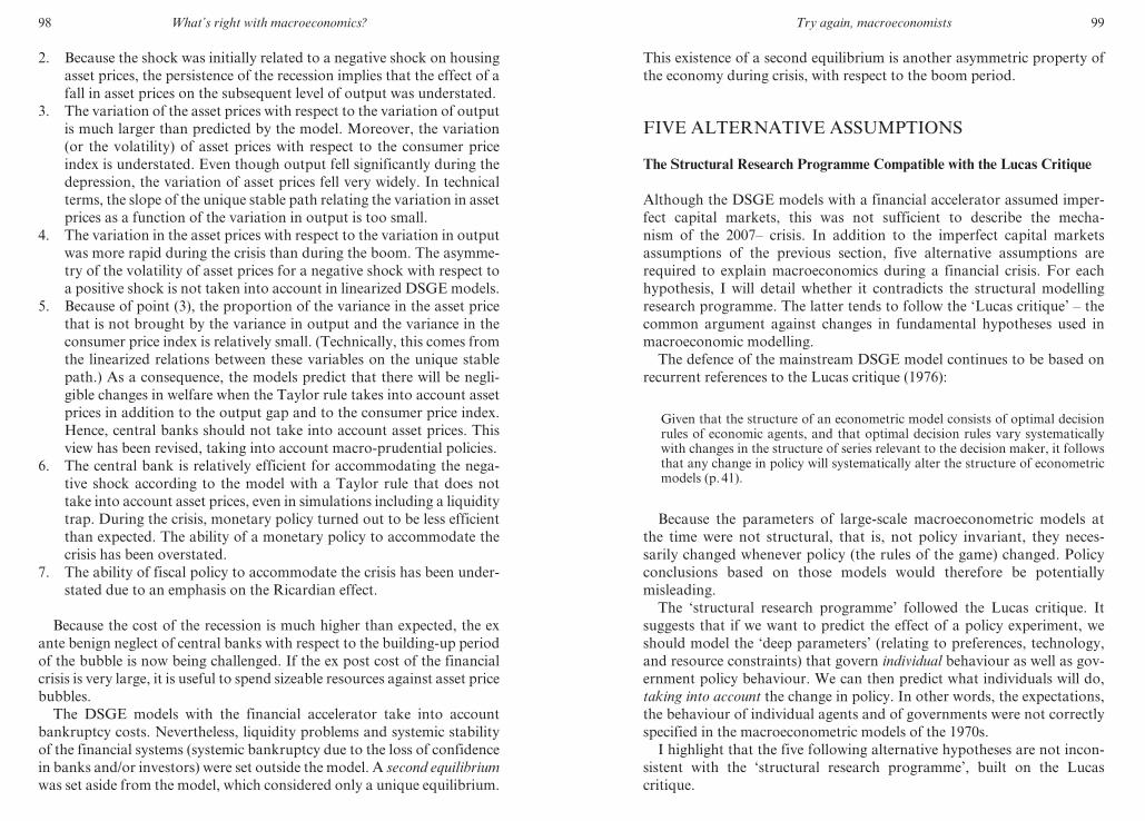
98 What’s right with macroeconomics?
2. Because the shock was initially related to a negative shock on housing
asset prices, the persistence of the recession implies that the effect of a
fall in asset prices on the subsequent level of output was understated.
3. The variation of the asset prices with respect to the variation of output
is much larger than predicted by the model. Moreover, the variation
(or the volatility) of asset prices with respect to the consumer price
index is understated. Even though output fell significantly during the
depression, the variation of asset prices fell very widely. In technical
terms, the slope of the unique stable path relating the variation in asset
prices as a function of the variation in output is too small.
4. The variation in the asset prices with respect to the variation in output
was more rapid during the crisis than during the boom. The asymme-
try of the volatility of asset prices for a negative shock with respect to
a positive shock is not taken into account in linearized DSGE models.
5. Because of point (3), the proportion of the variance in the asset price
that is not brought by the variance in output and the variance in the
consumer price index is relatively small. (Technically, this comes from
the linearized relations between these variables on the unique stable
path.) As a consequence, the models predict that there will be negli-
gible changes in welfare when the Taylor rule takes into account asset
prices in addition to the output gap and to the consumer price index.
Hence, central banks should not take into account asset prices. This
view has been revised, taking into account macro- prudential policies.
6. The central bank is relatively efficient for accommodating the nega-
tive shock according to the model with a Taylor rule that does not
take into account asset prices, even in simulations including a liquidity
trap. During the crisis, monetary policy turned out to be less efficient
than expected. The ability of a monetary policy to accommodate the
crisis has been overstated.
7. The ability of fiscal policy to accommodate the crisis has been under-
stated due to an emphasis on the Ricardian effect.
Because the cost of the recession is much higher than expected, the ex
ante benign neglect of central banks with respect to the building- up period
of the bubble is now being challenged. If the ex post cost of the financial
crisis is very large, it is useful to spend sizeable resources against asset price
bubbles.
The DSGE models with the financial accelerator take into account
bankruptcy costs. Nevertheless, liquidity problems and systemic stability
of the financial systems (systemic bankruptcy due to the loss of confidence
in banks and/or investors) were set outside the model. A second equilibrium
was set aside from the model, which considered only a unique equilibrium.
M3014 - SOLOW TEXT.indd 98 21/11/2012 13:03
Try again, macroeconomists 99
This existence of a second equilibrium is another asymmetric property of
the economy during crisis, with respect to the boom period.
FIVE ALTERNATIVE ASSUMPTIONS
The Structural Research Programme Compatible with the Lucas Critique
Although the DSGE models with a financial accelerator assumed imper-
fect capital markets, this was not sufficient to describe the mecha-
nism of the 2007– crisis. In addition to the imperfect capital markets
assumptions of the previous section, five alternative assumptions are
required to explain macroeconomics during a financial crisis. For each
hypothesis, I will detail whether it contradicts the structural modelling
research programme. The latter tends to follow the ‘Lucas critique’ – the
common argument against changes in fundamental hypotheses used in
macroeconomic modelling.
The defence of the mainstream DSGE model continues to be based on
recurrent references to the Lucas critique (1976):
Given that the structure of an econometric model consists of optimal decision rules of economic agents, and that optimal decision rules vary systematically with changes in the structure of series relevant to the decision maker, it follows that any change in policy will systematically alter the structure of econometric models (p. 41).
Because the parameters of large- scale macroeconometric models at
the time were not structural, that is, not policy invariant, they neces-
sarily changed whenever policy (the rules of the game) changed. Policy
conclusions based on those models would therefore be potentially
misleading.
The ‘structural research programme’ followed the Lucas critique. It
suggests that if we want to predict the effect of a policy experiment, we
should model the ‘deep parameters’ (relating to preferences, technology,
and resource constraints) that govern individual behaviour as well as gov-
ernment policy behaviour. We can then predict what individuals will do,
taking into account the change in policy. In other words, the expectations,
the behaviour of individual agents and of governments were not correctly
specified in the macroeconometric models of the 1970s.
I highlight that the five following alternative hypotheses are not incon-
sistent with the ‘structural research programme’, built on the Lucas
critique.
M3014 - SOLOW TEXT.indd 99 21/11/2012 13:03

100 What’s right with macroeconomics?
Hypothesis 1: A Second Equilibrium with Systemic Bankruptcy is Possible
First, the financial accelerator is a partial summarization of Irving Fisher’s
ideas. Ben Bernanke is one of the most eminent scholars on the subject,
given his long interest in the crisis of the 1930s and his revival of Fisher’s
debt deflation ideas during the last 30 years. Bernanke and Mark Gertler
(2000), however, proposed this misleading statement of a posteriori man-
agement of asset price bubbles by central banks, without ex ante control
of asset price bubbles:
We explore the implications of asset price volatility for the management of monetary policy. We show that it is desirable for central banks to focus on underlying inflationary pressures. Asset prices become relevant only to the extent they may signal potential inflationary or deflationary forces. Rules that directly target asset prices appear to have undesirable side effects. We base our conclusions on (i) simulation of different policy rules in a small scale macro model and (ii) a comparative analysis of recent US and Japanese monetary policy (p. 2).
A central claim for this error is that it came from a common misun-
derstanding of Fisher’s (1933) ideas as being only related to a financial
accelerator that amplifies technological and productivity shocks leading
to over- investment, such as the new car industry in the 1920s, the Internet
industry in the 1990s, and so on. For Gottfried Haberler (1937 [1946]) it
is clear that:
over- investment rather than over- indebtedness is the primary cause of the breakdown . . . We may thus conclude that the ‘debt- factor’ plays an independ-ent role as intensifier of the depression, but can hardly be regarded as an inde-pendent cause of the breakdown. (Chapter 4, pp. 115–16)
Fisher (1933), however, also makes the frequent comparison to the
‘capsizing’ of a ship:
To take another simile, such a disaster is somewhat like the ‘capsizing’ of a ship which, under ordinary conditions, is always near stable equilibrium but which, after being tipped beyond a certain angle, has no longer this tendency to return to equilibrium, but, instead, a tendency to depart from it. (p. 339)
Small waves make the ship oscillate around Fisher’s first equilibrium,
inside a ‘stability corridor’. By analogy, this describes regular economic
cycles, not large crises. Large waves, on the other hand, make the ship
pass below a threshold angle and capsize (a second equilibrium). This is a
low- level equilibrium related to ‘economic instability’. Hence, Fisher’s is
M3014 - SOLOW TEXT.indd 100 21/11/2012 13:03
Try again, macroeconomists 101
not only a story of amplified oscillation around a single equilibrium (in a
corridor of stability), it is also a story of bifurcation toward a second bad
equilibrium (‘instability’) – an autarky with an overall risk of macroeco-
nomic bankruptcy, a breakdown of the financial system and low produc-
tion levels. This equilibrium may also be related to low- equilibrium bank
runs as dealt with by Douglas Diamond and Philip Dybvig (1983) in the
field of the microeconomics of banking. The economy may only be able
to pass the downward threshold (the threshold angle for the boat) leading
to the second bad equilibrium due to the over- lending amplification of
over- investment. Otherwise, over- investment theories alone may lead only
to minor shocks, and the economy remains in the stability corridor. Since
without the financial accelerator the shift to the low equilibrium (‘instabil-
ity’) is unlikely to occur, over- lending is then a cause of the breakdown.
Let us look at a graphical, dynamic model representing a possible rela-
tionship between asset prices at the current date q(t) and asset prices at
the next date q(t11). Starting from the equilibrium E1, if a small negative
shock on the asset price q(t) occurs, such that q(t) is equal to B, then the
economy will exhibit small fluctuations around the stable equilibrium E1.
These fluctuations occur in a corridor of stability.
If, however, a large negative shock occurs, such that the asset price q(t)
is below the value of a second unstable equilibrium E2, then the asset price
dynamics follow a different decreasing and diverging path towards a third
equilibrium that is also stable, where the asset price is equal to zero.
Until recently, modern mainstream macroeconomics dealing with the
financial accelerator very rarely considered this second equilibrium.
Hyman Minsky’s (1982) question, ‘Can it happen again?’, referring to
the 1929 crisis, was answered as ‘Never’. This argument was based on
an under- valuation of the probability of a world financial crisis: the prob-
ability was assumed to be close to zero. It was also based on an under-
valuation of the ex post cost of a world financial crisis. For example, the
evaluation of the costs of a financial crisis in developed countries such as
Sweden in the 1990s were two to five times less than the costs incurred by
emerging economies such as Argentina. This was also backed by Lucas’s
(1987) small valuation of business cycles’ loss of welfare for a representa-
tive agent with a constant intertemporal elasticity of substitution. In 2010,
central bankers changed their views and considered the possibility of
macro- prudential regulation policies.
The problem highlighted is not that bankruptcy costs were missing
in the financial accelerator. What is missing is systemic bankruptcy
due to expectations of a high probability of default caused by a lack of
confidence.
The Lucas critique does not assume that there are never multiple
M3014 - SOLOW TEXT.indd 101 21/11/2012 13:03
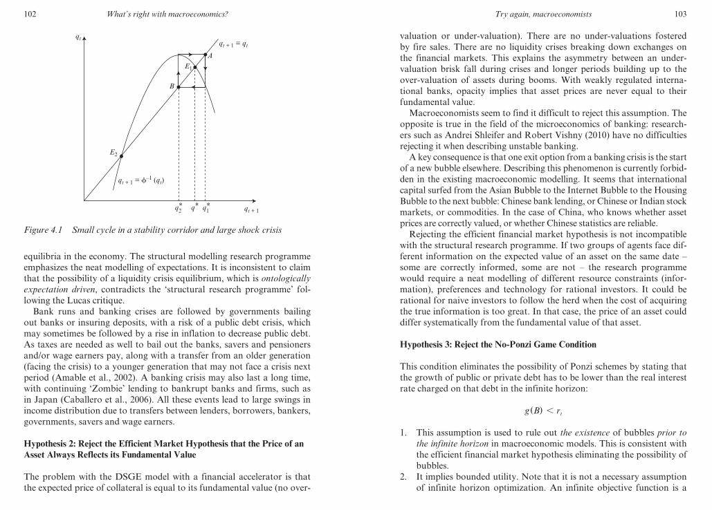
102 What’s right with macroeconomics?
equilibria in the economy. The structural modelling research programme
emphasizes the neat modelling of expectations. It is inconsistent to claim
that the possibility of a liquidity crisis equilibrium, which is ontologically
expectation driven, contradicts the ‘structural research programme’ fol-
lowing the Lucas critique.
Bank runs and banking crises are followed by governments bailing
out banks or insuring deposits, with a risk of a public debt crisis, which
may sometimes be followed by a rise in inflation to decrease public debt.
As taxes are needed as well to bail out the banks, savers and pensioners
and/or wage earners pay, along with a transfer from an older generation
(facing the crisis) to a younger generation that may not face a crisis next
period (Amable et al., 2002). A banking crisis may also last a long time,
with continuing ‘Zombie’ lending to bankrupt banks and firms, such as
in Japan (Caballero et al., 2006). All these events lead to large swings in
income distribution due to transfers between lenders, borrowers, bankers,
governments, savers and wage earners.
Hypothesis 2: Reject the Efficient Market Hypothesis that the Price of an
Asset Always Reflects its Fundamental Value
The problem with the DSGE model with a financial accelerator is that
the expected price of collateral is equal to its fundamental value (no over-
qt + 1 = �–1 (qt)
qt + 1 = qt
qt + 1
qt
q1*q2
* q*
E2
E1
B
A
Figure 4.1 Small cycle in a stability corridor and large shock crisis
M3014 - SOLOW TEXT.indd 102 21/11/2012 13:03
Try again, macroeconomists 103
valuation or under- valuation). There are no under- valuations fostered
by fire sales. There are no liquidity crises breaking down exchanges on
the financial markets. This explains the asymmetry between an under-
valuation brisk fall during crises and longer periods building up to the
over- valuation of assets during booms. With weakly regulated interna-
tional banks, opacity implies that asset prices are never equal to their
fundamental value.
Macroeconomists seem to find it difficult to reject this assumption. The
opposite is true in the field of the microeconomics of banking: research-
ers such as Andrei Shleifer and Robert Vishny (2010) have no difficulties
rejecting it when describing unstable banking.
A key consequence is that one exit option from a banking crisis is the start
of a new bubble elsewhere. Describing this phenomenon is currently forbid-
den in the existing macroeconomic modelling. It seems that international
capital surfed from the Asian Bubble to the Internet Bubble to the Housing
Bubble to the next bubble: Chinese bank lending, or Chinese or Indian stock
markets, or commodities. In the case of China, who knows whether asset
prices are correctly valued, or whether Chinese statistics are reliable.
Rejecting the efficient financial market hypothesis is not incompatible
with the structural research programme. If two groups of agents face dif-
ferent information on the expected value of an asset on the same date –
some are correctly informed, some are not – the research programme
would require a neat modelling of different resource constraints (infor-
mation), preferences and technology for rational investors. It could be
rational for naive investors to follow the herd when the cost of acquiring
the true information is too great. In that case, the price of an asset could
differ systematically from the fundamental value of that asset.
Hypothesis 3: Reject the No- Ponzi Game Condition
This condition eliminates the possibility of Ponzi schemes by stating that
the growth of public or private debt has to be lower than the real interest
rate charged on that debt in the infinite horizon:
g(B) , rt
1. This assumption is used to rule out the existence of bubbles prior to
the infinite horizon in macroeconomic models. This is consistent with
the efficient financial market hypothesis eliminating the possibility of
bubbles.
2. It implies bounded utility. Note that it is not a necessary assumption
of infinite horizon optimization. An infinite objective function is a
M3014 - SOLOW TEXT.indd 103 21/11/2012 13:03

104 What’s right with macroeconomics?
possible solution, as in the Ramsey model (1928). If one maximizes
discounted utility over time, why should one refuse infinite utility?
3. It is a key assumption to obtain Ricardian equivalence (for example,
the inefficiency of budgetary policy financed by debt and followed by
taxes later on) (Barro, 1974). The assumption is related to an infinite
horizon government solvency. This may be different from short- run
solvency, however. Imagine that we apply a similar reasoning to that
in the financial accelerator: public debt is solvent based on expected
taxes net of public expenditures:
(1 1 rt) # Bt , tt11
# Yt(1 1 gt11
(Y)) 2 Gt(1 1 gt11
(Y))
If the expected growth of output is large and if the interest rate on
public bonds is low, this solvency constraint is likely to be respected.
This is what bond holders may think about in the short run. They
would like taxes to increase and public expenditures to fall, but would
enjoy more output growth, which increases the tax base.
Imagine that that is the case for all future periods. Then, for all
dates, the public debt is ‘short- term’ solvent. Imagine that at the same
time, the growth rate of output is equal to the growth rate of public
debt, but is larger than the real interest rate on public debt. Then, the
‘infinite horizon’ (no- Ponzi game) solvency constraint is not fulfilled,
whereas the short- run solvency constraint is always fulfilled. In this
case, the infinite horizon solvency constraint is meaningless. Utility
is unbounded. In this context, one does not know whether Ricardian
equivalence holds or not.
4. In the endogenous growth literature, balanced growth implies that
debt grows at the same rate as output. This equation is inconsistent
with growth miracles lasting more than 20 years, where the growth of
output consistently exceeds the real rate of interest for several decades
(Japan 1960–90; China 1990–2010) (Amable et al., 2010):
g(B) 5 g(Y) , rt
If the non- efficient financial market hypothesis is consistent with
the research programme following the Lucas critique, then one could
reject the no- Ponzi game condition.
Hypothesis 4: Reject the Unique Stable Path Dynamics
Intertemporal optimization with a discount rate leads nearly always
to saddle- path dynamics, with only one path having a stable lower
M3014 - SOLOW TEXT.indd 104 21/11/2012 13:03
Try again, macroeconomists 105
dimension. All the others are unstable. A rational expectation hypothesis
rules out all unstable paths by assumption. It is an additional assumption
with respect to the Lucas critique. A consequence is that, for the same
optimizing model, the volatility of asset prices on this path is much lower
than that on the others.
The linearization around the equilibrium of the unique stable path
leading to a unique long- term equilibrium reduces the study of macroeco-
nomic dynamics to dampened responses of macroeconomic variables to
small shocks.
The first point: rejecting the unique equilibrium goes along with
accepting the ‘expectation- driven’ liquidity crisis alternative equilibrium.
Multiple equilibria driven by expectations are consistent with the research
programme.
The second point: the unique stable path goes along with the no- Ponzi
game condition, which rules out that the economy follows temporary
bubble paths for asset prices prior to the infinite horizon. That means
that all agents know when an asset price is on a bubble path, and that
they decide ex ante never to be on the unstable path. Nevertheless, let us
imagine the scheme proposed, for example, by Shleifer and Vishny (2010)
on rational unstable banking. A number of naive investors do not know
that the asset is not correctly priced. Knowledgeable investors (banks)
expect that a boom with over- priced assets will be followed by a crisis with
under- priced assets. In that context, it is easy to compute the conditions
for more informed rational banks to speculate.
Linearization considers only small shocks, which do not correspond
to recessions. It leads to a repetitive representation of macroeconomic
dynamics as dampened responses to small shocks. Along with the multi-
ple equilibria hypothesis, large shocks are likely to shift the regime of the
economy, and the dynamics will differ dramatically.
Hypothesis 5: Reject the Unconstrained Consumption- smoothing Euler
Equation
The unconstrained Euler equation for households, where the growth of
consumption is determined only as an increasing function of the rate of
interest on savings, decreases with the aversion to consumption volatility:
g(C) 5rt 2 r
s
This equation is rarely challenged in macroeconomic textbooks, yet
1. it does not match the data (Caroll, 1997);
M3014 - SOLOW TEXT.indd 105 21/11/2012 13:03
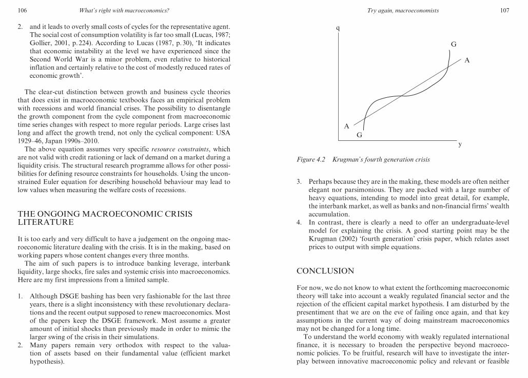
106 What’s right with macroeconomics?
2. and it leads to overly small costs of cycles for the representative agent.
The social cost of consumption volatility is far too small (Lucas, 1987;
Gollier, 2001, p. 224). According to Lucas (1987, p. 30), ‘It indicates
that economic instability at the level we have experienced since the
Second World War is a minor problem, even relative to historical
inflation and certainly relative to the cost of modestly reduced rates of
economic growth’.
The clear- cut distinction between growth and business cycle theories
that does exist in macroeconomic textbooks faces an empirical problem
with recessions and world financial crises. The possibility to disentangle
the growth component from the cycle component from macroeconomic
time series changes with respect to more regular periods. Large crises last
long and affect the growth trend, not only the cyclical component: USA
1929–46, Japan 1990s–2010.
The above equation assumes very specific resource constraints, which
are not valid with credit rationing or lack of demand on a market during a
liquidity crisis. The structural research programme allows for other possi-
bilities for defining resource constraints for households. Using the uncon-
strained Euler equation for describing household behaviour may lead to
low values when measuring the welfare costs of recessions.
THE ONGOING MACROECONOMIC CRISIS LITERATURE
It is too early and very difficult to have a judgement on the ongoing mac-
roeconomic literature dealing with the crisis. It is in the making, based on
working papers whose content changes every three months.
The aim of such papers is to introduce banking leverage, interbank
liquidity, large shocks, fire sales and systemic crisis into macroeconomics.
Here are my first impressions from a limited sample.
1. Although DSGE bashing has been very fashionable for the last three
years, there is a slight inconsistency with these revolutionary declara-
tions and the recent output supposed to renew macroeconomics. Most
of the papers keep the DSGE framework. Most assume a greater
amount of initial shocks than previously made in order to mimic the
larger swing of the crisis in their simulations.
2. Many papers remain very orthodox with respect to the valua-
tion of assets based on their fundamental value (efficient market
hypothesis).
M3014 - SOLOW TEXT.indd 106 21/11/2012 13:03
Try again, macroeconomists 107
3. Perhaps because they are in the making, these models are often neither
elegant nor parsimonious. They are packed with a large number of
heavy equations, intending to model into great detail, for example,
the interbank market, as well as banks and non- financial firms’ wealth
accumulation.
4. In contrast, there is clearly a need to offer an undergraduate- level
model for explaining the crisis. A good starting point may be the
Krugman (2002) ‘fourth generation’ crisis paper, which relates asset
prices to output with simple equations.
CONCLUSION
For now, we do not know to what extent the forthcoming macroeconomic
theory will take into account a weakly regulated financial sector and the
rejection of the efficient capital market hypothesis. I am disturbed by the
presentiment that we are on the eve of failing once again, and that key
assumptions in the current way of doing mainstream macroeconomics
may not be changed for a long time.
To understand the world economy with weakly regulated international
finance, it is necessary to broaden the perspective beyond macroeco-
nomic policies. To be fruitful, research will have to investigate the inter-
play between innovative macroeconomic policy and relevant or feasible
AG
G
A
y
q
Figure 4.2 Krugman’s fourth generation crisis
M3014 - SOLOW TEXT.indd 107 21/11/2012 13:03

108 What’s right with macroeconomics?
banking and financial regulatory policy at the micro level, as well as politi-
cal economy issues.
REFERENCES
Amable, B., J- B. Chatelain and O. De Bandt (2002), ‘Optimal capacity in the banking sector and economic growth’, Journal of Banking and Finance, 26(2–3), 491–517.
Amable, B., J- B. Chatelain and K. Ralf (2010), ‘Patents as collateral’, Journal of Economic Dynamics and Control, 34(6), 1092–104.
Barro, R.J. (1974), ‘Are government bonds net wealth?’, The Journal of Political Economy, 82(6), 1095–117.
Bernanke, B. and M. Gertler (2000), ‘Monetary policy and asset price volatility’, NBER Working Paper 7559.
Bernanke, B. and M. Gertler (2001), ‘Should central banks respond to movements in asset prices?’, American Economic Review, 91(2), 253–57.
Bernanke, B., M. Gertler and S. Gilchrist (1999), ‘The financial accelerator in a quantitative business cycle framework’, Handbook of Macroeconomics, Amsterdam: Elsevier, pp. 1341–93.
Borio, C.E.V. and P.W. Lowe (2002), ‘Asset prices, financial and monetary stabil-ity: exploring the nexus’, BIS Working Paper 114.
Caballero, R.J., T. Hoshi and A.K. Kashyap (2006), ‘Zombie lending and depressed restructuring in Japan’, NBER Working Paper 12129.
Caroll, C.D. (1997), ‘Death to the log- linearized consumption Euler equation! (and very poor health to the second- order approximation)’, NBER Working Paper 6298.
Diamond, D.W. and P.H. Dybvig (1983), ‘Bank runs, deposit insurance and liquidity’, The Journal of Political Economy, 91(3), 401–19.
Fisher, I. (1933), ‘The debt- deflation theory of great depressions’, Econometrica, 1(4), 337–57.
Gollier, C. (2001), The Economics of Risk and Time, Cambridge, MA: MIT Press.Haberler, G. (1937 [1946]), Prosperity and Depression: A Theoretical Analysis of
Cyclical Movements, 3rd edn, New York: United Nations, Lake Success.Iacoviello, M. (2005), ‘House prices, borrowing constraints, and monetary policy
in the business cycle’, American Economic Review, 95(3), 739–64.Kiyotaki, N. and J.H. Moore (1997), ‘Credit cycles’, Journal of Political Economy,
105(2), 211–48.Krugman, P. (2002), ‘Crisis: the next generation?’, in Economic Policy in the
International Economy: Essays in Honor of Assaf Razin, Cambridge: Cambridge University Press, pp. 15–32.
Lucas, R.E. (1976), ‘Econometric policy evaluation: a critique’, Carnegie- Rochester Conference Series on Public Policy, 1, 19–46.
Lucas, R.E. (1987), Models of Business Cycles, Oxford: Basil Blackwell.Miller, M. and J. Stiglitz (2010), ‘Leverage and asset bubbles: averting
Armageddon with chapter 11’, Economic Journal, 120(544), 500–518.Minsky, H.P. (1982), Can ‘it’ Happen Again?: Essays on Instability and Finance,
Armonk, NY: M.E. Sharpe.Rajan, R.G. and L. Zingales (2003), ‘The great reversals: the politics of financial
M3014 - SOLOW TEXT.indd 108 21/11/2012 13:03
Try again, macroeconomists 109
development in the twentieth century’, Journal of Financial Economics, 69(1), 5–50.
Ramsey, F.P. (1928), ‘A mathematical theory of saving’, Economic Journal, 38(152), 543–59.
Reinhart, C.M. and K. Rogoff (2009), This Time is Different, Eight Centuries of Financial Folly, Princeton, NJ: Princeton University Press.
Shleifer, A. and R. Vishny (2010), ‘Unstable banking’, Journal of Financial Economics, 97(3), 306–18.
Smets, F. and R. Wouters (2003), ‘An estimated dynamic stochastic general equi-librium model for the euro area’, Journal of the European Economic Association, 1(5), 1123–75.
M3014 - SOLOW TEXT.indd 109 21/11/2012 13:03

110
5. Economic policies with endogenous innovation and Keynesian demand management1
Giovanni Dosi, Giorgio Fagiolo,
Mauro Napoletano and Andrea Roventini
INTRODUCTION
The global crisis has strikingly brought to the fore the importance of
banking and financial markets for the dynamics of real economies. It has
also revealed itself to be a ‘natural experiment’ for economic analysis,
exposing the inadequacy of the predominant theoretical frameworks. The
basic assumptions of mainstream models2 – such as rational expectations,
optimizing, representative agents, and so on – are to a large extent respon-
sible for the failure to forecast the crisis. They also seem to be unable to
propose a remedy for putting economies back on a steady growth path
(Colander et al., 2008; Kirman, 2010). In fact, the crisis sets a tall chal-
lenge for alternative, evolutionary theories, linking micro behaviour and
aggregate dynamics.
In this chapter, we develop an evolutionary, agent- based model to try
to fill the theoretical vacuum present nowadays in macroeconomics. The
model addresses three major, interrelated, questions. First, it explores the
processes by which technological change affects macro variables, such as
unemployment, output fluctuations and average growth rates. In addition
to this ‘Schumpeterian’ question, we also ask how such endogenous, firm-
specific changes in the supply side of the economy interact with demand
conditions. This is a basic ‘Keynesian’ issue. Finally, we explore the pos-
sible existence of long- term effects of demand variations. Is long- term
growth only driven by changes in technology, or does aggregate demand
affect future dynamics? Are there multiple growth paths whose selection
depends on demand and institutional conditions?
To do so, we refine and expand the model in Dosi et al. (2010),3 which
we use also as a sort of ‘policy laboratory’ where both business cycle and
growth effects of different public policies can be evaluated under diverse
M3014 - SOLOW TEXT.indd 110 21/11/2012 13:03
Economic policies with endogenous innovation 111
institutional scenarios. In this respect, the model makes it possible to
experiment with an ensemble of policies related to the supply side of the
economy (for example, technology), as well as to the macro- management
demand side (for example, fiscal and monetary policies).
From a historical perspective, a separation has emerged in macro-
economics: growth theories have tried to explain the trends present in
macro time series, whereas business cycle models have accounted for the
observed fluctuations around the trend. The IS–LM interpretation of
John Maynard Keynes (Hicks, 1937) and growth models rooted in the
seminal work of Robert Solow (1956) are prominent examples of such a
division of labour.
In the business cycle theoretical camp, different theories have been
competing over time. On the one hand, ‘New Classical’ and ‘Real Business
Cycle (RBC) theories’ have considered irrelevant any ‘Keynesian’ feature
of the economy. On the other hand, New Keynesians have stressed the
importance of aggregate demand shocks in economic fluctuations, often
relying on nominal and real rigidities as well as on informational and
behavioural frictions (see Blanchard, 2009, for an insightful overview),
with just a small subset of them considering such ‘imperfections’ as struc-
tural, long- term characteristics of the economy (see, for example, Akerlof
and Yellen, 1985; Greenwald and Stiglitz, 1993a, 1993b; Akerlof, 2002,
2007).
More recently, the New Neoclassical Synthesis between real busi-
ness cycle and a major breed of New Keynesian models – rooted in the
dynamic stochastic general equilibrium (DSGE) models (see Woodford,
2003; Galí and Gertler, 2007) – has added modest quantities of Keynesian
elements to an otherwise supply- side model of economic fluctuations.
The backbone of DSGE models is indeed a RBC model augmented with
sticky prices, imperfect competition, monetary- policy (Taylor- like) rules,
and any other possible types of imperfections.4 DSGE models, however,
are not suited to deal with long- run growth issues since their RBC core
prevents them from exploring any Schumpeterian source of endogenous
innovation.
On the opposite side, endogenous growth models (see Romer, 1990;
Aghion and Howitt, 1992; Dinopoulos and Segerstrom, 1999) have a
Schumpeterian core, which makes innovation and the ensuing dynamics
in technology endogenous. There is no room, however, for demand- driven
fluctuations in this set of models, even if some of them (for example,
Aghion and Howitt, 1998; Aghion et al., 2010; Aghion and Marinescu,
2007; Aghion et al., 2008) allow for equilibrium fluctuations wherein
Keynesian features do not have any role.
This issue is also present in evolutionary models (Nelson and Winter,
M3014 - SOLOW TEXT.indd 111 21/11/2012 13:03

112 What’s right with macroeconomics?
1982). They are driven indeed by a Schumpeterian engine with endog-
enous innovations, but they do not take sufficiently into account any
demand- related forces affecting macroeconomic activity.5
Our model has evolutionary roots. It explicitly accounts for an endog-
enous technological search, heterogeneous ‘boundedly rational’ agents
and competitive dynamics entailing some form of market selection across
firms, and through that, across technologies – all fundamental building
blocks of evolutionary interpretations of economic dynamics (following
the seminal Nelson and Winter, 1982). Unlike most ‘first generation’
evolutionary models, however, it abandons any assumption of market
clearing on the labour or the product markets. In line with some New
Keynesian insights (see, for example Stiglitz, 1994), it tries to study the
feedbacks between the factors affecting aggregate demand and those
influencing technological change. This allows us to develop a unified
framework where one can jointly study long- term dynamics and business
cycles.
The model belongs to the growing literature on agent- based compu-
tational economics (ACE) (see Tesfatsion and Judd, 2006; LeBaron and
Tesfatsion, 2008), and it thus allows for many heterogeneous agents who
interact without any ex ante commitment to the reciprocal consistency
of their actions (for example, market clearing).6 The model thus satisfies
Robert Solow’s call for micro heterogeneity (Solow, 2008).
Furthermore, the model, in line with most agent- based models (ABMs),
is based on a ‘realistic’ representation of what agents do, how they adjust,
and so on. In that, it provides an explicit microfoundation of macro
dynamics. At the same time, we try to describe micro behaviours as closely
as possible to the available micro- empirical evidence. This is in line with
George Akerlof’s plea for ‘behavioural microeconomics’ (Akerlof, 2002).
In this way, we reduce our degrees of freedom in modelling agents’ behav-
iour. Moreover, we test the capability of the model to jointly account
for a large set of stylized facts related to ‘micro/meso’ aggregates (for
example, firm size and growth- rate distributions, productivity dispersions,
firm investment patterns) together with macro- statistical properties (for
example, persistent output growth, output volatility, unemployment rates,
and so on).
The model portrays an artificial economy composed of capital- and
consumption- good firms, workers, a bank, and the public sector. Capital-
goods firms perform research and development (R&D) and produce
heterogeneous machine tools. Consumption- goods firms invest in new
machines and produce a homogeneous consumption good. Firms finance
their production and investment choices employing internal funds as
well as credit provided by the banking sector. Finally, the public sector
M3014 - SOLOW TEXT.indd 112 21/11/2012 13:03
Economic policies with endogenous innovation 113
levies taxes on firms’ profits and workers’ wages and pays unemployment
benefits.
As every ABM, the properties of the model must be analysed via
extensive computer simulations. To overcome the usual problems,
shared by many ABMs, related to parameterization sensitivity,7 we
look for policy results that: (i) are robust to reasonable changes in the
parameters of the model; (ii) stem from model set- ups and parameter-
izations wherein the output of the model is empirically validated (that
is, the statistical properties of simulated microeconomic and macroeco-
nomic data are similar to those observed in reality). We think that this
is a positive feature of our study, because very often in the literature,
no empirical validation constraints are imposed on policy experiment
results (Fukac and Pagan, 2006; Canova, 2008; Fagiolo and Roventini,
2012). Moving to the normative side, different ‘control’ parameters and
institutional, market, or industry set- ups can mimic different public pol-
icies, whose impact is then quantitatively assessed by employing ensuing
aggregates, such as average output growth, output volatility, average
unemployment, and so on.
Extensive empirical validation exercises show that the model is able to
deliver self- sustaining patterns of growth characterized by the presence of
endogenous business cycles. Moreover, the model is also able to replicate
the most important stylized facts concerning macroeconomic dynamics
(for example, cross- correlations, relative volatilities), as well as micro-
economic dynamics (such as firm size distributions, firm productivity
dynamics, firm investment patterns).
Our policy- simulation exercises show a strong complementarity between
Schumpeterian technology policies and Keynesian fiscal policies. Both
types of policies are needed to put the economy onto a long- run steady
growth path. Schumpeterian policies foster economic growth, but they are
not able alone to sustain long- run high economic growth patterns char-
acterized by mild business cycle fluctuations and low unemployment. If
Keynesian policies are present, Schumpeterian policies also affect the per-
formance of the economy in the short run, contributing to the reduction
in output volatility and unemployment. Moreover, Keynesian policies
are the best instrument for tackling short- run problems, having a strong
impact on output volatility and unemployment. We show that monetary
policy can have strong effects on growth as well. In particular, high inter-
est rates not only exacerbate volatility and unemployment rates, but also
are capable of worsening the long- run growth prospects of the economy.
Our results also point to a strong interplay between monetary policy and
the income distribution characteristics of the economy. More specifically,
on the one hand, income distributions that are more favourable to wages
M3014 - SOLOW TEXT.indd 113 21/11/2012 13:03

114 What’s right with macroeconomics?
stabilize aggregate consumption demand and lower both volatility and
unemployment. On the other hand, lower profit rates magnify the effects
of changes in interest rates by increasing the dependence of firms on
external financing from the bank.
The chapter is organized as follows. We first describe the model. Next,
we perform empirical validation checks and present results of policy
exercises. The final section concludes and discusses future extensions.
THE MODEL
The economy is composed of a machine- producing sector made of F1
firms (denoted by the subscript i), a consumption- goods sector made of F2
firms (denoted by the subscript j), L s consumers/workers, a bank, and a
public sector. Capital- goods firms invest in R&D and produce heterogene-
ous machines. Consumption- goods firms combine machine tools bought
from capital- goods firms and labour in order to produce a final product
for consumers. The bank provides credit to firms using firms’ savings.
Credit is allotted to firms on a pecking- order basis according to their net
worth. Moreover, the supply and the dynamics of debt of the firms in the
economy can be influenced by various policy instruments (capital require-
ments, mandatory reserves, interest rates). Finally, the public sector levies
taxes on firms’ profits and pays unemployment benefits.
The Timeline of Events
In any given time period (t), the following microeconomic decisions take
place in sequential order.
1. Policy variables (for example, the central bank interest rate, the
reserve requirement, the tax rate, unemployment benefits, and so on)
are fixed.
2. Total credit provided by the bank to each firm is determined.
3. Machine- tool firms perform R&D to try to discover new products and
more efficient production techniques and to imitate the technology
and the products of their competitors. Capital- goods firms advertise
their machines with consumption- goods firms.
4. Consumption- goods firms buy the machines ordered in the previous
period and decide how much to produce and invest. If internal funds
are not enough, firms borrow from the bank. If investment is posi-
tive, consumption- goods firms choose their supplier and send in their
orders.
M3014 - SOLOW TEXT.indd 114 21/11/2012 13:03
Economic policies with endogenous innovation 115
5. In both industries, firms hire workers according to their production
plans and start producing.
6. An imperfectly competitive consumption- goods market opens.
The market shares of firms evolve according to their price com-
petitiveness.
7. Firms in both sectors compute their profits. If profits are positive,
firms pay back their loans to the bank and deposit their savings.
8. Entry and exit take place. In both sectors, firms with near zero market
shares and negative net worth are eschewed from their industry and
replaced by new firms.
9. Machines ordered at the beginning of the period are delivered and
become part of the capital stock at time t 1 1.
At the end of each time step, aggregate variables (for example, gross
domestic product [GDP], investment, employment) are computed,
summing up the corresponding microeconomic variables.
The Capital- goods Industry
The technology of a capital- goods firm is (Ati ,B
ti) , where the former coeffi-
cient stands for the labour productivity of the machine tool manufactured
by i for the consumption- goods industry (a rough measure of producer
quality), while the latter coefficient is the labour productivity of the pro-
duction technique employed by firm i itself. The positive integer t denotes
the current technology vintage. Given the monetary wage w, the unit cost
of production of a capital- goods firm is:
ci(t) 5
w(t)
Bti
(5.1)
With a fixed mark- up (m1 . 0) pricing rule,8 prices (pi) are defined as:
pi(t) 5 (1 1 m1
)ci(t) (5.2)
The unit labour cost of production in the consumption- goods sector
associated with each machine of vintage t, produced by firm i is:
c(Ati , t) 5
w(t)
Ati
Firms in the capital- goods industry ‘adaptively’ strive to increase their
market share and profits to try to improve their technology via innovation
M3014 - SOLOW TEXT.indd 115 21/11/2012 13:03
116 What’s right with macroeconomics?
and imitation. Both are costly processes. Firms invest in R&D a fraction
of their past sales (Si) :
RDi(t) 5 vSi
(t 2 1) (5.3)
with 0 , v , 1. R&D expenditures are used to hire researchers, who are
paid the market wage w(t) .9 Firms split their R&D efforts between inno-
vation (IN) and imitation (IM) according to the parameter x [ [0,1]:10
INi(t) 5 xRDi
(t)
IMi(t) 5 (1 2 x)RDi
(t)
We model innovation as a two- step process. The first step determines
whether or not a firm obtains an access to innovation – irrespective of
whether it is ultimately a success or a failure – through a draw from a
Bernoulli distribution, whose parameter qini
(t) is given by:
qini
(t) 5 1 2 e2z1INi(t) (5.4)
with 0 , z1 # 1. Note that according to (5.4), there are some scale- related
returns to R&D investment: access to innovative discoveries is more likely
if a firm puts more resources into R&D. If a firm innovates, it may draw a
new machine embodying technology (Aini , Bin
i) according to:
Aini
(t) 5 Ai(t) (1 1 xA
i(t))
Bini
(t) 5 Bi(t) (1 1 xB
i(t))
where xAi and xB
i are two independent draws from a Beta (a1, b1) distribu-
tion over the support [x1, x1] with x1 belonging to the interval [21, 0] and
x1 to [0, 1]. Note that the notional possibilities of technological advance
– that is, technological opportunities – are captured by the support of the
Beta distribution and by its shape. So, for example, with low opportuni-
ties, the largest probability density falls over ‘failed’ innovations – that is,
potential capital goods that are ‘worse’ in terms of costs and performance
than those already produced by the searching firm. Conversely, under a
condition of rich opportunities, innovations that dominate incumbent
technologies will be drawn with high probability. As we shall show below,
a crucial role of ‘Schumpeterian’ technology policies is precisely that of
influencing opportunities and micro capabilities.
Like the innovation search, imitation follows a two- step procedure.
M3014 - SOLOW TEXT.indd 116 21/11/2012 13:03
Economic policies with endogenous innovation 117
The possibilities of accessing imitation come from sampling a Bernoulli
(qimi
(t)) :
qimi
(t) 5 1 2 e2z2IMi(t) (5.5)
with 0 , z2 # 1. Firms accessing the second stage are able to copy the
technology of one of their competitors (Aimi , Bim
i) . We assume that firms
are more likely to imitate competitors with similar technologies, and we
use Euclidean metrics to compute the technological distance between
every pair of firms to weigh imitation probabilities.
All firms that draw a potential innovation or imitation have to
put it on production or keep producing the incumbent generation of
machines. Comparing the different technologies competing for adop-
tion, firms choose to manufacture the machine characterized by the best
trade- off between price and efficiency. More specifically, knowing that
consumption- goods firms invest following a payback period routine (see
below), capital- goods firms select the machine to produce according to the
following rule:
min [phi(t) 1 bch (Ah
i , t) ], h 5 t, in, im (5.6)
where b is a positive payback period parameter (see equation (5.10)
below). Once the type of machine is chosen, we capture the imperfect
information pervading the market, assuming that each firm sends a
‘brochure’ with the price and the productivity of its offered machines
to both its historical (HCi) clients and to a random sample of poten-
tial new customers (NCi) , whose size is proportional to HCi (that is,
NCi(t) 5 gHCi
(t) , with 0 , g , 1).
The Consumption- goods Industry
Consumption- goods firms produce homogeneous goods using capital
(that is, their stock of machines) and labour under constant returns to
scale. Firms plan their production (Qj) according to adaptive demand
expectations (Dej) :
Dej(t) 5 f(Dj
(t 2 1), Dj(t 2 2), . . ., Dj
(t 2 h)) (5.7)
where Dj(t 2 1) is the demand actually faced by firm j at time t 2 1 (h
positive integer).11 The desired level of production (Qdj) depends on the
expected demand as well as on the desired inventories (Ndj) and the actual
stock of inventories Nj:
M3014 - SOLOW TEXT.indd 117 21/11/2012 13:03

118 What’s right with macroeconomics?
Qdj(t) 5 De
j(t) 1 Nd
j(t) 2 Nj
(t 2 1) (5.8)
with Ndj(t) 5 iDe
j(t) , i [ [0, 1]. The output of consumption- goods firms
is constrained by their capital stock (Kj) . If the desired capital stock (Kd
j)
– computed as a function of the desired level of production – is higher
than the current capital stock, firms invest (EIdj) in order to expand their
production capacity:12
EIdj(t) 5 Kd
j(t) 2 Kj
(t) (5.9)
The capital stock of each firm is obviously composed of heterogeneous
vintages of machines with different productivity. We define Xj(t) as the
set of all vintages of machine tools belonging to firm j at time t. Firms
scrap machines following a payback period routine. Through that, techni-
cal change and equipment prices influence the replacement decisions of
consumption- goods firms.13 More specifically, firm j replaces machine
Ati [ Xj
(t) according to its technology obsolescence as well as the price of
new machines:
RSj(t) 5 eAt
i [ Xj(t) :
p*(t)
c(Ai,t, t) 2 c*(t)# b f (5.10)
where p* and c* are the price and unit cost of production for the new
machines. Firms compute their replacement investment by summing up
the number of old machine tools that satisfy equation (5.10).14
Consumption- goods firms choose their capital- goods supplier by com-
paring the price and productivity of the currently manufactured machine
tools that they know of. As mentioned above (in ‘The Capital- goods
Industry’), the capital- goods market is systematically characterized by
imperfect information. This implies that consumption- goods firms compare
‘brochures’ that describe the characteristics of machines only from a subset
of equipment suppliers. Firms then choose the machines with the lowest
price and unit cost of production (that is, pi(t)1bc(At
i , t)) and send their
orders to the corresponding machine manufacturer. Machine production is
a time- consuming process: capital- goods firms deliver the ordered machine
tools at the end of the period.15 Gross investment of each firm (Ij) is the sum
of expansion and replacement investment. By pooling the investment of all
consumption- goods firms, one gets aggregate investment (I).
Consumption- goods firms have to finance their investments as well as
their production, as they advance worker wages. In line with a growing
number of theoretical and empirical papers (see, for example, Stiglitz and
Weiss, 1992; Greenwald and Stiglitz, 1993a; Hubbard, 1998), we assume
M3014 - SOLOW TEXT.indd 118 21/11/2012 13:03
Economic policies with endogenous innovation 119
imperfect capital markets. This implies that the financial structure of
firms matters (external funds are more expensive than internal ones), and
firms may be credit rationed. More specifically, consumption- goods firms
finance production using their stock of liquid assets (NWj) . If liquid assets
do not fully cover production costs, firms borrow the remaining part from
a bank, paying an interest rate rL. The maximum amount of credit lent by
the bank to firm j(TCj) is a positive function of the firm’s stock of liquid
assets, as well as its size proxied by its past sales (see ‘The Banking Sector’
below). Only firms that are not production rationed can try to fulfil their
investment plans by employing their residual stock of liquid assets first,
and then their residual borrowing capacity.16
Given their current stock of machines, consumption- goods firms
compute average productivity (pj) and unit cost of production (cj
) . Prices
are set by applying a variable mark- up (mj) on unit costs of production:
pj(t) 5 (1 1 mj
(t))cj(t) (5.11)
Mark- up variations are regulated by the evolution of firms’ market shares
( fj
) :17
mj(t) 5 mj
(t 2 1) a1 1 vfj
(t 2 1) 2 fj(t 2 2)
fj(t 2 2)
bwith 0 # v # 1.
The consumption- goods market is also characterized by imperfect infor-
mation.18 This implies that consumers do not instantaneously switch to
products made by more competitive firms. Prices, however, are clearly one
of the key determinants of firms’ competitiveness (Ej) . The other component
is the level of unfulfilled demand (lj) inherited from the previous period:
Ej(t) 5 2 w1pj
(t) 2 w2lj(t) (5.12)
where w1,2 are positive parameters.19 Weighting the competitiveness of
each consumption- goods firm by its past market share ( fj) , one can
compute the average competitiveness of the consumption- goods sector:
E(t) 5 aF2
j51
Ej(t) fj
(t 2 1)
Such variables also represent a moving selection criterion driving, other
things being equal, expansions, contractions and extinctions within the
population of firms. We parsimoniously model this market set- up, letting
M3014 - SOLOW TEXT.indd 119 21/11/2012 13:03

120 What’s right with macroeconomics?
firms’ market shares evolve according to a ‘quasi’ replicator dynamic (for
antecedents in the evolutionary camp, see Silverberg et al., 1988; Metcalfe,
1994a):
fj(t) 5 fj
(t 2 1) a1 1 cEj
(t) 2 E(t)
E(t)b (5.13)
with c . 0.20
The profits (Pj) of each consumption- goods firm read:
Pj(t) 5 Sj
(t) 2 cj(t)Qj
(t) 2 rLDebj(t) 1 rDNWj
(t 2 1)
where Sj(t) 5 pj
(t)Dj(t) and Debj
(t) denote the stock of debt. The invest-
ment choices of each firm and its profits determine the evolution of its
stock of liquid assets (NWj) :
NWj(t) 5 NWj
(t 2 1) 1 Pj(t) 2 cIj
(t)
where cIj is the amount of internal funds employed by firm j to finance
investment.
The Banking Sector
In the banking sector, there is only one commercial bank (or n commercial
banks that are equal) that gathers deposits and provides credit to firms. In
what follows, we first describe how total credit is determined by the bank,
and how credit is allocated to each firm. We then move on to describe the
organization of the credit flow in the economy and the balance sheet of
the bank. Finally, we describe how profits and net worth of the bank are
determined.
The maximum credit available in the economy is set by the credit multi-
plier. More precisely, in each period, the bank reinvests in credit the funds
obtained through deposits from firms. This amount of credit returns to the
bank in the form of deposits. The bank then subtracts from this amount
the mandatory reserve and lends the remainder, which returns again in the
form of deposits, and so on. If we let aR be the mandatory reserve coeffi-
cient, then total deposits obtained from the above procedure, Dep(t 2 1),
are determined as:
Dep(t 2 1) 5aN1
i51NWi
(t 2 1) 1 aN2
j51NWj
(t 2 1)
aR
, 0 # aR # 1
(5.14)
M3014 - SOLOW TEXT.indd 120 21/11/2012 13:03
Economic policies with endogenous innovation 121
where gN1
i51NWi
(t 2 1) and gN2
j51NWj
(t 2 1) are the total net worth of
upstream and downstream firms at time t 2 1.
From the above equation, it follows that total credit available in the
economy at time t, MTC(t) is:
MTC(t) 5 (1 2 aR)Dep(t 2 1) (5.15)
Total credit is allocated to each firm in the consumption- goods sector
on a pecking- order basis, according to the ratio between stock of liquid
assets and sales, NWj (t)
Sj(t) . More precisely, the bank first ranks firms on the
basis of their stock of liquid assets- to- sales ratio; then it starts to satisfy
the demand of the first firm in the rank, then the second one, and so on. If
the total credit available is insufficient to fulfil the demand of all the firms
in the pecking order list, the firms that are credit rationed go bankrupt. On
the other hand, the total demand for credit can also be lower than the total
supply of credit. In this case, all demands of firms in the pecking order are
fulfilled, and no firm goes bankrupt. It follows that in any period the stock
of loans of the bank satisfies the following constraint:
aN2
j51Debj
(t) 5 Loan(t) # TC(t) (5.16)
The profits of the bank are equal to interest rate receipts from redeem-
able loans and from interest on reserves held at the central bank minus
interest paid on deposits. Furthermore, the bank fixes its deposit and loan
rates by applying respectively a mark- down and a mark- up on the central
bank rate r. For simplicity, we assume that bank reserves, Cash(t) , are
remunerated at the same rate as deposits:
rD 5 (1 2 yD)r, 0 # yD # 1 (5.17)
rL 5 (1 1 yL)r, 0 # yL # 1 (5.18)
From the above hypotheses it follows that the expression for the bank’s
profits, pb (t) is:
pb (t) 5 rLLoan(t) 2 rDDep(t) 1 rDCash(t 2 1) (5.19)
To complete the description of the banking sector, we need to determine
the bank’s net worth at the end of the period, NWb (t) . The net worth of
the bank is equal to the stock of liquid assets of the bank minus the stock
of bad debt accumulated up to time t, that is, BD(t) . Liquid assets are
M3014 - SOLOW TEXT.indd 121 21/11/2012 13:03

122 What’s right with macroeconomics?
given by the stock of cash accumulated up to time t, plus the profits of the
period. Accordingly, the expression for the net worth of the bank reads as:
NWb (t) 5 Cash(t) 1 pb (t) 2 BD(t) 5 NWb (t 2 1) 1 DCash(t)
1 pb (t) 2 BD(t) (5.20)
The bank goes bankrupt if its net worth becomes negative. Note that
this allows us to appreciate the difference between liquidity and solvency
risks, which has been a hot topic during the crisis. Similar to what hap-
pened in the post-2007 financial turmoil, we assume that the insolvency of
the bank is solved by allowing the public sector to buy the bank’s bad debt.
Schumpeterian Exit and Entry Dynamics
At the end of each period, a firm exits for two reasons: (i) competition,
that is, the firm has a (quasi) zero market share; or (ii) bankruptcy, that
is, the firm’s net worth becomes negative and the bank is not willing to
provide additional credit. If a firm fails, the bank’s stock of bad debt is
increased accordingly.
We keep the number of firms fixed, hence any dead firm is replaced
by a new one. Furthermore, in line with the empirical literature on firm
entry (Caves, 1998; Bartelsman et al., 2005), we assume that entrants
are on average smaller than incumbents, with the stock of capital of new
consumption- goods firms and the stock of liquid assets of entrants in
both sectors being a fraction of the average of that of the incumbents.21
Concerning the technology of entrants, new consumption- goods firms
select amongst the newest vintages of machines, according to the ‘bro-
chure mechanism’ described above. The process- and product- related
knowledge of new capital- goods firms is drawn from a Beta distribution,
whose shape and support is shifted and ‘twisted’ according to whether
entrants enjoy an advantage or a disadvantage vis- à- vis incumbents.22 In
fact, the distribution of opportunities for entrants versus incumbents is a
crucial characteristic of different sectoral technological regimes and plays
a role somewhat akin to the distance from the technological frontier of
entrants discussed in Aghion and Howitt (2007).
The Labour Market
The labour market is certainly not Walrasian: real wages do not clear
the market, and involuntary unemployment as well as labour rationing
are the rules rather than the exceptions. The aggregate labour demand
M3014 - SOLOW TEXT.indd 122 21/11/2012 13:03
Economic policies with endogenous innovation 123
(L D) is computed by summing up the labour demand of capital- and
consumption- goods firms. The aggregate supply (L S) is exogenous and
inelastic. Hence, aggregate employment (L) is the minimum between L D
and L S.
The wage rate is a function of institutional and market factors, with
both indexation mechanisms on consumption prices and average produc-
tivity, on the one hand, and adjustments to unemployment rates, on the
other:
Dw(t)
w(t 2 1)5 ga Dcpi(t)
cpi(t 2 1),
DAB(t)
AB(t 2 1),
DU(t)
U(t 2 1)b (5.21)
where cpi is the consumer price index, AB the average labour productivity,
and U the unemployment rate.23
Consumption, Taxes and Public Expenditures
An otherwise black- boxed public sector levies taxes on firm profits
and worker wages or on profits only and pays to unemployed
workers a subsidy (wu) , which is a fraction of the current market wage
(that is, wu (t) 5 fw(t) , with f [ (0,1)). In fact, taxes and subsidies are
the fiscal levers that contribute to the aggregate demand management
regimes.
Aggregate consumption (C) depends on the income of both employed
and unemployed workers as well as on past savings:
C(t) 5 c [w(t)L D(t) 1 wu (L
S 2 L D(t)) 1 rD
(1 2 c)C(t 2 1) ] (5.22)
where 0 , c # 1 is the marginal propensity to consume (in the present
set- up c 5 1). The model satisfies the standard national account identities:
the sum of the value added of capital- and consumption- goods firms (Y)
equals their aggregate production, since in our simplified economy, there
are no intermediate goods; that in turn coincides with the sum of aggregate
consumption, investment and change in inventories (DN) :
aF1
i51
Qi(t) 1 a
F2
j51
Qj(t) 5 Y(t) ; C(t) 1 I(t) 1 DN(t)
The dynamics generated at the micro level by decisions of a multiplicity
of heterogeneous, adaptive agents and by their interaction mechanisms is
the explicit microfoundation of the dynamics for all aggregate variables of
interest (for example, output, investment, employment, and so on).
M3014 - SOLOW TEXT.indd 123 21/11/2012 13:03

124 What’s right with macroeconomics?
EMPIRICAL VALIDATION
The foregoing model does not allow for analytical, closed- form solu-
tions. This general ABM distinctive feature stems from the non- linearities
present in agent decision rules and their interaction patterns. It also forces
us to run computer simulations to analyse the properties of the stochastic
processes governing the co- evolution of micro and macro variables.24 In
what follows, we therefore perform extensive Monte Carlo analyses to
wash away cross- simulation variability. Consequently, all results below
refer to averages taken from over a hundred Monte Carlo replications.25
Let us start from a sort of ‘benchmark’ set- up for which the model is
empirically validated, meaning it is studied in its ability to replicate a wide
spectrum of microeconomic and macroeconomic stylized facts. Initial con-
ditions and parameters of the benchmark set- up are presented in Table 5.1.
As already mentioned, the model embodies both a Schumpeterian engine
and a Keynesian one. The former belongs to the generation of innovations
created by an ensemble of equipment producers that expensively search
for and endogenously differentiate between the technology they are able to
master. The Keynesian engine has two parts: a direct one – through fiscal
policies – and an indirect one – via investment decisions and workers’ con-
sumption. Hence, the benchmark model appropriately embodies all such
Schumpeterian and Keynesian features.
Next, we tune, so to speak, ‘up’ and ‘down’ the key policy variables
(for example, tax rates, unemployment benefits, interest rates), and we
experiment with different conditions affecting the access to and exploita-
tion of new technological opportunities (for example, the patent regime,
anti- trust policies) or the distribution of income between profits and wages
(mark- up rates of firms).
Let us first explore the ability of the model to reproduce the major styl-
ized facts regarding both the properties of macroeconomic aggregates and
the underlying distribution of micro characteristics (for more on both in
the direct antecedents to this model, see Dosi et al., 2006, 2008).
Growth and Fluctuations
The model is able to robustly generate endogenous, self- sustained growth
patterns characterized by the presence of persistent fluctuations (see
Figure 5.1). At business cycle frequencies, the bandpass- filtered output
(Bpf), investment and consumption series (Bpf: see, for example, Baxter
and King, 1999) display the familiar ‘roller- coaster’ dynamics (see Figure
5.2) observed in real data (see, for example, Stock and Watson, 1999;
Napoletano et al., 2006). Moreover, in tune with the empirical evidence,
M3014 - SOLOW TEXT.indd 124 21/11/2012 13:03
Economic policies with endogenous innovation 125
both consumption and investment appear to be procyclical variables, with
the latter series being also more volatile than GDP.
The insights coming from visual inspection of time series data are
confirmed by more quantitative analyses. Table 5.2 reports descriptive
statistics on output, consumption and investment time series. As the table
clearly shows, output, consumption and investment display strictly posi-
tive average growth rates26 and, according to the Dickey–Fuller tests, they
seem to exhibit a unit root. After detrending the series with a bandpass
filter, we compute standard deviations and cross- correlations between
Table 5.1 Benchmark parameters
Description Symbol Value
Number of firms in capital- goods industry F1 50
Number of firms in consumption- goods industry F2 200
R&D investment propensity n 0.04
R&D allocation to innovative search x 0.50
Firm search capabilities parameters z 0.30
Beta distribution parameters (innovation process) (a1, b1) (3, 3)
Beta distribution support (innovation process) [x1, x1] [20.15, 0.15]
New- customer sample parameter g 0.50
Capital- goods firm mark- up rule m1 0.10
Desired inventories i 0.10
Payback period b 3
‘Physical’ scrapping age h 20
Mark- up coefficient n 0.01
Competitiveness weights w1, 2 1
Replicator dynamics coefficient c 1
Uniform distribution supports (consumption- goods
entrant capital)
[�1, �2] [0.10,0.90]
Uniform distribution supports (entrant stock of
liquid assets)
[�3, �4] [0.10,0.90]
Beta distribution parameters (capital- goods
entrants technology)
(a1, b2) (2, 4)
Wage setting DAB weight y1 1
Wage setting Dcpi weight y2 0
Wage setting DU weight y3 0
Tax rate tr 0.10
Unemployment subsidy rate f 0.40
Maximum debt/sales ratio L 2
Interest rate r 0.025
Bank mark- up coefficient yL 0.50
Bank mark- down coefficient yD 1
M3014 - SOLOW TEXT.indd 125 21/11/2012 13:03

126 What’s right with macroeconomics?
00
5
10
15
20
25
50 100 150 200 250Time
GDPInv.Cons.
Logs
300 350 400 450
Figure 5.1 Level of output, investment and consumption (logs)
0–1
–0.8
–0.6
–0.4
–0.2
0
0.2
0.4
0.6
0.8
1.0
50 100 150 200 250 300 350 400 450Time
GDPInv.Cons.
Figure 5.2 Bandpass- filtered output, investment and consumption
M3014 - SOLOW TEXT.indd 126 21/11/2012 13:03
Economic policies with endogenous innovation 127
output and the other series (see respectively Tables 5.2 and 5.3). In line
with the empirical literature on business cycles (see, for example, Stock
and Watson, 1999), in our model, investment is also more volatile than
output, whereas consumption is less so; consumption, investment, change
in inventories, and employment are procyclical; unemployment is coun-
tercyclical. Consumption and net investment are also coincident variables
matching yet another empirical regularity in business cycles. Changes in
inventories are instead slightly lagging.27
Furthermore, the model is also able to match the business- cycle proper-
ties concerning productivity, labour market, and price variables (see Table
5.3). Indeed, productivity is procyclical; prices are countercyclical and
leading; inflation is procyclical and lagging; mark- ups are strongly coun-
tercyclical (for the empirics and discussion, see Stock and Watson, 1999;
Rotemberg and Woodford, 1999).
The model is also in line with the major business cycle stylized facts con-
cerning credit (see Table 5.3). Indeed, firms’ total debt displays a strong
procyclical character. In addition, its fluctuations are contemporaneous
to output movements. The cross- correlations in Table 5.3 also shed light
on the characteristics of the credit dynamics underneath business cycles in
the model, which has strong ‘Minskian’ features (see Minsky, 1986). First,
bank deposits are countercyclical and lag GDP. Moreover, bankruptcy
rates are procyclical and lag GDP dynamics very closely. This behaviour
is mapping the evolution of firms’ financial health over the cycle. At the
onset of an expansionary phase, firms’ profits and cash flows improve.
This pushes higher production and investment expenditures, therefore
Table 5.2 Output, investment and consumption statistics
Output Consumption Investment
Avg. growth rate 0.0254
(0.0002)
0.0252
(0.0002)
0.0275
(0.0004)
Dickey–Fuller test (logs) 6.7714
(0.0684)
9.4807
(0.0957)
0.2106
(0.0633)
Dickey–Fuller test (Bpf) −6.2564*
(0.0409)
−5.8910*
(0.0447)
−6.8640*
(0.0905)
Std. Dev. (Bpf) 0.0809
(0.0007)
0.0679
(0.0005)
0.4685
(0.0266)
Rel. Std. Dev. (output) 1 0.8389 5.7880
Notes:
Bpf: bandpass- filtered (6,32,12) series.
Monte- Carlo simulation standard errors in parentheses.
(*): Significant at 5%.
M3014 - SOLOW TEXT.indd 127 21/11/2012 13:03

128
Ta
ble
5.3
C
orr
ela
tio
n s
tru
ctu
re
Ser
ies
Ou
tpu
t
(Bp
f)
(Bp
f)t-
4t-
3t-
2t-
1t
t11
t12
t13
t14
Ou
tpu
t−
0.1
022
(0.0
090)
0.1
769
(0.0
080)
0.5
478
(0.0
048)
0.8
704
(0.0
014)
1 (0)
0.8
704
(0.0
014)
0.5
478
(0.0
048)
0.1
769
(0.0
080)
−0.1
022
(0.0
090)
Co
nsu
mp
tio
n−
0.1
206
(0.0
123)
0.0
980
(0.0
129)
0.4
256
(0.0
106)
0.7
563
(0.0
062)
0.9
527
(0.0
017)
0.9
248
(0.0
018)
0.6
848
(0.0
038)
0.3
394
(0.0
058)
0.0
250
(0.0
072)
Inves
tmen
t−
0.2
638
(0.0
102)
−0.3
123
(0.0
137)
−0.2
646
(0.0
182)
−0.0
864
(0.0
210)
0.1
844
(0.0
206)
0.4
473
(0.0
175)
0.5
950
(0.0
139)
0.5
757
(0.0
123)
0.4
206
(0.0
129)
Net
In
ves
tmen
t−
0.0
838
(0.0
122)
0.0
392
(0.0
167)
0.2
195
(0.0
216)
0.4
010
(0.0
235)
0.5
114
(0.0
211)
0.5
037
(0.0
153)
0.3
850
(0.0
103)
0.2
105
(0.0
112)
0.0
494
(0.0
138)
Ch
. in
in
ves
tmen
t0.0
072
(0.0
081)
0.1
184
(0.0
070)
0.2
349
(0.0
060)
0.2
948
(0.0
072)
0.2
573
(0.0
090)
0.1
331
(0.0
098)
−0.0
199
(0.0
097)
−0.1
319
(0.0
085)
−0.1
640
(0.0
067)
Em
plo
ym
ent
−0.3
240
(0.0
087)
−0.1
901
(0.0
123)
0.0
796
(0.0
151)
0.4
083
(0.0
160)
0.6
692
(0.0
149)
0.7
559
(0.0
120)
0.6
451
(0.0
084)
0.4
067
(0.0
069)
0.1
555
(0.0
082)
Un
emp
l. r
ate
0.3
357
(0.0
083)
0.2
084
(0.0
118)
−0.0
596
(0.0
147)
−0.3
923
(0.0
158)
−0.6
607
(0.0
148)
−0.7
550
(0.0
120)
−0.6
489
(0.0
084)
−0.4
112
(0.0
070)
−0.1
583
(0.0
082)
M3014 - SOLOW TEXT.indd 128 21/11/2012 13:03
129
Pro
du
ctiv
ity
0.1
180
(0.0
097)
0.3
084
(0.0
088)
0.5
316
(0.0
092)
0.7
108
(0.0
093)
0.7
672
(0.0
076)
0.6
656
(0.0
067)
0.4
378
(0.0
097)
0.1
664
(0.0
126)
−0.0
609
(0.0
128)
Pri
ce0.2
558
(0.0
167)
0.3
181
(0.0
218)
0.2
702
(0.0
235)
0.0
916
(0.0
216)
−0.1
645
(0.0
198)
−0.3
950
(0.0
212)
−0.5
067
(0.0
225)
−0.4
688
(0.0
210)
−0.3
249
(0.0
176)
Infl
ati
on
−0.1
070
(0.0
151)
0.0
841
(0.0
135)
0.3
110
(0.0
175)
0.4
456
(0.0
226)
0.4
021
(0.0
228)
0.1
966
(0.0
188)
−0.0
628
(0.0
154)
−0.2
478
(0.0
146)
−0.2
900
(0.0
131)
Mark
- up
0.2
183
(0.0
118)
0.1
599
(0.0
088)
0.0
411
(0.0
128)
−0.0
988
(0.0
184)
−0.2
040
(0.0
213)
−0.2
361
(0.0
206)
−0.1
968
(0.0
174)
−0.1
226
(0.0
135)
−0.0
580
(0.0
107)
To
tal
deb
t0.1
225
(0.0
249)
0.2
460
(0.0
229)
0.3
793
(0.0
211)
0.4
848
(0.0
216)
0.5
250
(0.0
238)
0.4
824
(0.0
253)
0.3
691
(0.0
243)
0.2
203
(0.0
212)
0.0
763
0.0
173
Ban
k d
epo
sits
−0.0
907
(0.0
215)
−0.2
375
(0.0
171)
−0.3
659
(0.0
127)
−0.4
322
(0.0
118)
−0.4
154
(0.0
144)
−0.3
264
(0.0
168)
−0.2
001
(0.0
171)
−0.0
760
(0.0
157)
0.0
196
0.0
138
Ban
kru
ptc
y r
ate
0.1
077
(0.0
082)
0.2
667
(0.0
120)
0.3
827
(0.0
159)
0.4
104
(0.0
178)
0.3
424
(0.0
170)
0.2
132
(0.0
144)
0.0
776
(0.0
127)
−0.0
202
(0.0
128)
−0.0
667
(0.0
132)
No
tes:
Bp
f: b
an
dp
ass
- fil
tere
d (
6,3
2,1
2)
seri
es.
Mo
nte
- Ca
rlo
sim
ula
tio
n s
tan
da
rd e
rro
rs i
n p
are
nth
eses
.
M3014 - SOLOW TEXT.indd 129 21/11/2012 13:03

130 What’s right with macroeconomics?
inducing a rise in firms’ debt. In turn, the rise in the cost of debt gradually
erodes firms’ cash flows and savings, therefore leading to higher bank-
ruptcy ratios and setting the premises for the incoming recession phase.
Distributions of Microeconomic Characteristics
Together with the ability of the model to account for a rich ensemble of
macro phenomena, how does it fare in replicating cross- sectional evi-
dence on firms’ dynamics? Let us consider the regularities concerning
firm- size and growth- rate distributions, firm- productivity dynamics, firm-
investment and firm- bankruptcy patterns generated by the model.
Figures 5.3 and 5.4 show the rank- size plot of the pooled firm size in the
capital- goods and consumption- goods sectors. As the plots indicate quite
starkly, firm size distributions are right- skewed in both cases, and thus
in tune with empirical evidence (Dosi, 2007). In addition, this qualitative
evidence is reinforced by the analysis of firms’ growth rates (not shown),
which display fat tails in both sectors.
40
1
2
3
4
5
6
7
8
6 8 10 12 14log (Size)
Empirical
LogNormal
16 18 20 22 24
log
(Ran
k)
Figure 5.3 Pooled (year- standardized) capital- goods firms’ sales
distributions: log rank vs. log size plots
M3014 - SOLOW TEXT.indd 130 21/11/2012 13:03
Economic policies with endogenous innovation 131
Turning to firm productivity and investment, again in line with the
empirical evidence (see the surveys in Bartelsman and Doms, 2000; Dosi,
2007), firms differ strikingly in terms of labour productivity in both sectors
(see the standard deviations in labour productivity across firms plotted in
Figure 5.5). Furthermore, the model is able to generate, as an emergent
property, investment lumpiness (Doms and Dunne, 1998; Caballero,
1999). Indeed, in each time step, consumption- goods firms with very low
investment levels coexist with firms experiencing investment spikes (see
Figure 5.6, in relation to Gourio and Kashyap, 2007).
Finally, we have analysed firm bankruptcy patterns. The recent evidence
on this issue (see, for example, Fujiwara, 2004; Di Guilmi et al., 2004) has
pointed out that the distribution of bankruptcy rates is highly skewed to
the right and fat tailed, also displaying power- law- like behaviour. This
implies that business cycles are typically characterized by episodes of
large bankruptcy avalanches. As the plots in Figure 5.7 clearly show, this
empirical evidence is well replicated by our model.
0
1
2
3
4
5
6
7
8
9
10
12 14log (Size)
Empirical
LogNormal
16 18 20 22 24
log
(Ran
k)
Figure 5.4 Pooled (year- standardized) consumption- goods firms’ sales
distributions: log rank vs. log size plots
M3014 - SOLOW TEXT.indd 131 21/11/2012 13:03
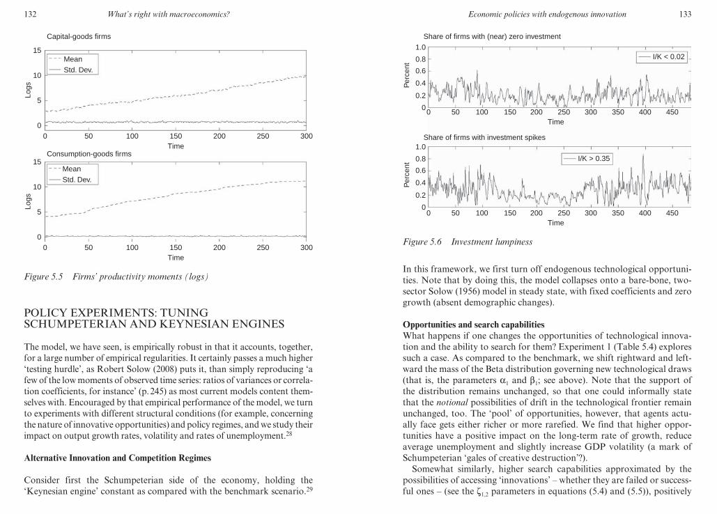
132 What’s right with macroeconomics?
POLICY EXPERIMENTS: TUNING SCHUMPETERIAN AND KEYNESIAN ENGINES
The model, we have seen, is empirically robust in that it accounts, together,
for a large number of empirical regularities. It certainly passes a much higher
‘testing hurdle’, as Robert Solow (2008) puts it, than simply reproducing ‘a
few of the low moments of observed time series: ratios of variances or correla-
tion coefficients, for instance’ (p. 245) as most current models content them-
selves with. Encouraged by that empirical performance of the model, we turn
to experiments with different structural conditions (for example, concerning
the nature of innovative opportunities) and policy regimes, and we study their
impact on output growth rates, volatility and rates of unemployment.28
Alternative Innovation and Competition Regimes
Consider first the Schumpeterian side of the economy, holding the
‘Keynesian engine’ constant as compared with the benchmark scenario.29
0
5
10
15
0 50Time
MeanStd. Dev.
100 150 200 250 300
Logs
0
5
10
15
0 50Time
MeanStd. Dev.
100 150 200 250 300
Logs
Capital-goods firms
Consumption-goods firms
Figure 5.5 Firms’ productivity moments (logs)
M3014 - SOLOW TEXT.indd 132 21/11/2012 13:03
Economic policies with endogenous innovation 133
In this framework, we first turn off endogenous technological opportuni-
ties. Note that by doing this, the model collapses onto a bare- bone, two-
sector Solow (1956) model in steady state, with fixed coefficients and zero
growth (absent demographic changes).
Opportunities and search capabilities
What happens if one changes the opportunities of technological innova-
tion and the ability to search for them? Experiment 1 (Table 5.4) explores
such a case. As compared to the benchmark, we shift rightward and left-
ward the mass of the Beta distribution governing new technological draws
(that is, the parameters a1 and b1; see above). Note that the support of
the distribution remains unchanged, so that one could informally state
that the notional possibilities of drift in the technological frontier remain
unchanged, too. The ‘pool’ of opportunities, however, that agents actu-
ally face gets either richer or more rarefied. We find that higher oppor-
tunities have a positive impact on the long- term rate of growth, reduce
average unemployment and slightly increase GDP volatility (a mark of
Schumpeterian ‘gales of creative destruction’?).
Somewhat similarly, higher search capabilities approximated by the
possibilities of accessing ‘innovations’ – whether they are failed or success-
ful ones – (see the z1,2 parameters in equations (5.4) and (5.5)), positively
00.2
0.40.60.81.0
0 50Time
I/K < 0.02
100 150 200 250 300 350 450400
Perc
ent
Share of firms with (near) zero investment
00.2
0.40.60.81.0
0 50Time
I/K > 0.35
100 150 200 250 300 350 450400
Perc
ent
Share of firms with investment spikes
Figure 5.6 Investment lumpiness
M3014 - SOLOW TEXT.indd 133 21/11/2012 13:03

134 What’s right with macroeconomics?
influence the rates of growth and lower unemployment. Together, busi-
ness cycle fluctuations are dampened possibly because a population of
‘more competent’ firms entails lower degrees of technological asymmetries
across them, and, indeed, also lower degrees of ‘creative destruction’. See
experiment 2, Table 5.4.
Note that such a role of innovative opportunities and search capabilities
is in principle equivalent to the one played by the more aggregate notions
of ‘human capital’ (Nelson and Phelps, 1966; Benhabib and Spiegel, 1994)
and ‘appropriate institutions’ (Acemoglu et al., 2006).30
Appropriability conditions
In many current models with a (neo) Schumpeterian engine, appropri-
ability conditions play a key role via their assumptions on the forward-
looking rationality of the agent(s) investing in an uncertain innovative
search: the degrees of monopoly appropriation of the economic benefits of
a successful search parameterize the equilibrium relation between invest-
ment in R&D and rates of innovation. In this model, we took a much
100
10–1
10–2
Pr (
X �
x)
10–3
10–4
10–5
10–1 100x
EmpPower Law Fit
Figure 5.7 Empirical distribution of consumption- goods firms’ bankruptcy
rate together with power- law fit
M3014 - SOLOW TEXT.indd 134 21/11/2012 13:03
135
Ta
ble
5.4
S
chu
mp
eter
ian
reg
ime
tech
no
log
ica
l a
nd
in
du
stri
al
po
licy
ex
per
imen
ts
Ex
per
imen
tD
escr
ipti
on
Av
g.
GD
P
Gro
wth
Ra
te
GD
P S
td.
Dev
. (B
pf)
Av
g.
Un
emp
loy
men
t
0b
ench
ma
rk s
cen
ari
o0
.02
54
(0.0
00
2)
0.0
80
9
(0.0
00
7)
0.1
07
2
(0.0
05
0)
1.1
low
tec
hn
olo
gic
al
op
po
rtu
nit
ies
0.0
19
5
(0.0
00
1)
0.0
79
4
(0.0
00
8)
0.1
35
7
(0.0
05
0)
1.2
hig
h t
ech
no
log
ica
l o
pp
ort
un
itie
s 0
.03
15
(0.0
00
2)
0.0
82
8
(0.0
00
7)
0.1
02
5
(0.0
05
1)
2.1
low
sea
rch
ca
pa
bil
itie
s0
.02
31
(0.0
00
2)
0.0
82
5
(0.0
00
8)
0.1
17
6
(0.0
05
9)
2.2
hig
h s
earc
h c
ap
ab
ilit
ies
0.0
26
8
(0.0
00
2)
0.0
77
5
(0.0
00
8)
0.1
03
1
(0
.00
48
)
3.1
pa
ten
t (l
eng
th o
nly
) 0
.02
42
(0.0
00
2)
0.0
76
1
(0.0
00
8)
0.1
13
2
(0.0
06
0)
3.2
pa
ten
t (b
rea
dth
, to
o)
0.0
16
3
(0.0
00
1)
0.0
63
1
(0.0
00
7)
0.1
32
9
(0.0
06
7)
4.1
low
en
tra
nt
exp
ecte
d p
rod
uct
ivit
y
0.0
18
3
(0.0
00
3)
0.0
79
8
(0.0
01
2)
0.1
40
2
(0.0
08
4)
4.2
hig
her
en
tra
nt
exp
ecte
d p
rod
uct
ivit
y
0.0
37
6
(0.0
00
2)
0.0
69
7
(0.0
00
6)
0.0
85
3
(0.0
04
7)
5.1
wea
k a
nti
tru
st
0.0
26
5
(0.0
00
2)
0.0
69
8
(0.0
00
6)
0.1
03
6
(0.0
04
3)
5.2
stro
ng
an
titr
ust
0
.02
73
(0.0
00
1)
0.0
50
8
(0.0
00
5)
0.0
83
7
(0.0
03
6)
6S
chu
mp
eter
- on
ly,
no
fis
cal
po
licy
0
.01
10
(0.0
01
8)
1.5
51
1
(0.0
42
7)
0.7
85
5
(0.0
27
4)
No
te:
Bp
f: b
an
dp
ass
- filt
ered
(6
,32
,12
) se
ries
. M
on
te- C
arl
o s
imu
lati
on
s st
an
da
rd e
rro
rs i
n p
are
nth
eses
.
M3014 - SOLOW TEXT.indd 135 21/11/2012 13:03

136 What’s right with macroeconomics?
more behavioural route and assumed a fixed propensity to invest in R&D.
Granted that, how do changes in appropriability conditions affect aggre-
gate dynamics?
We try to answer this question by mimicking the effect of a patent
system. Under a ‘length only’ patent scenario, the innovative technol-
ogy cannot be imitated for a given number of periods determined by the
patent length (see experiment 3.1, Table 5.4). Such patenting possibility
is detrimental to long- run growth and also augments the average rate of
unemployment. The negative aggregate impact of the patent system is
reinforced if each firm cannot innovate in some neighbourhood of the
other firms’ technologies – that is, in the presence of a patent breadth: see
experiment 3.2, Table 5.4.31
Entry and competition policies
Important dimensions of distinct Schumpeterian regimes of innovation
concern, first, the advantages/disadvantages that entrants face vis- à- vis
incumbents and, second, the market conditions placing economic rewards
and punishments on heterogeneous competitors.
The first theme cuts across the evolutionary and neo- Schumpeterian
literature and is sometimes dramatized as a ‘Schumpeterian Mark I’
versus a ‘Schumpeterian Mark II’ scenario, meaning systematic innova-
tive advantages for entrepreneurial entrants versus cumulative advantages
of incumbents (see Malerba and Orsenigo, 1995; Dosi et al., 1995). In our
model, technological entry barriers (or advantages) are captured by the
probability distribution over the ‘technological draws’ of entrants. Again,
we hold constant the support over which the economy (that is, every firm
therein) may draw innovative advances, conditional on the technology at
any time t. In this case, we do it for the sake of consistency: results apply
even more so if different regimes are also allowed to entail different prob-
ability supports. Let us first tune the Beta distribution parameters a2 and
b2 (see section on ‘Schumpeterian exit and entry dynamics’). Our results
are broadly in line with the evidence discussed in Aghion and Howitt
(2007): other things being equal, the easiness of entry and the competence
of entrants bear a positive impact on long- term growth, mitigate business
cycle fluctuations and reduce average unemployment. See experiments
4.1 and 4.2, Table 5.4. The ceteris paribus condition is equally important,
however: the same aggregate growth patterns can be proved to be equally
guaranteed by the competent, cumulative learning of incumbents (see
above the exercises on search capabilities).
What about competitive conditions? We introduce antitrust policies
by forbidding capital goods firms to exceed a given market share (75 per
cent in experiment 5.1 and 50 per cent in experiment 5.2, Table 5.4): the
M3014 - SOLOW TEXT.indd 136 21/11/2012 13:03
Economic policies with endogenous innovation 137
outcome is a lower unemployment rate, smaller business cycle fluctuations
and also higher GDP growth (on this point, see also Fogel et al., 2008).
Note that such a property has little to do with any static ‘welfare gains’ –
which our model does not explicitly contemplate – but it relates rather to
the multiplicity of producers, and thus of innovative search avenues, that
antitrust policies safeguard.32
Fiscal and Monetary Policies
We now focus on the effects of Keynesian policies. More precisely, fol-
lowing Dosi et al. (2010), we check whether the ‘Schumpeterian’ dynamics
embedded in the model is enough to generate sustained and steady growth,
or whether instead this can be reached only if Keynesian aggregate
demand policies are also well in place. Table 5.5 and Figure 5.8 present the
results of the experiments.
First, simulation results show that Keynesian policies have a strong
triggering effect on long- run average growth rates. If both the tax rate
and unemployment subsidy are set to zero, the economy is trapped in
an (almost) zero growth pattern characterized by extreme fluctuations
and persistently high unemployment. Tuning up fiscal policies releases
the economy from the ‘bad’ trajectory and puts it on the ‘good’ (high
growth) one, which our benchmark scenario also happens to belong to
(see Table 5.5 and Figure 5.8). If we further increase both the tax rate
Table 5.5 Keynesian regime fiscal policy experiments
Tax Rate Unemployment
Subsidy (in % of wages)
Avg. GDP
Growth Rate
GDP Std.
Dev. (Bpf)
Avg.
Unemployment
0 0 0.0035 1.5865 0.8868
(0.0012) (0.0319) (0.0201)
0.05 0.20 0.0254 0.1539 0.1952
(0.0002) (0.0025) (0.0086)
0.10 0.40 0.0252 0.0809 0.1072
(0.0002) (0.0007) (0.0050)
0.15 0.60 0.0251 0.0630 0.0846
(0.0002) (0.0005) (0.0034)
0.20 0.80 0.0254 0.0584 0.0602
(0.0002) (0.0006) (0.0027)
0.25 1 0.0252 0.0564 0.0551
(0.0002) (0.0005) (0.0023)
Note: Bpf: bandpass- filtered (6,32,12) series. Monte- Carlo simulations standard errors in
parentheses.
M3014 - SOLOW TEXT.indd 137 21/11/2012 13:03
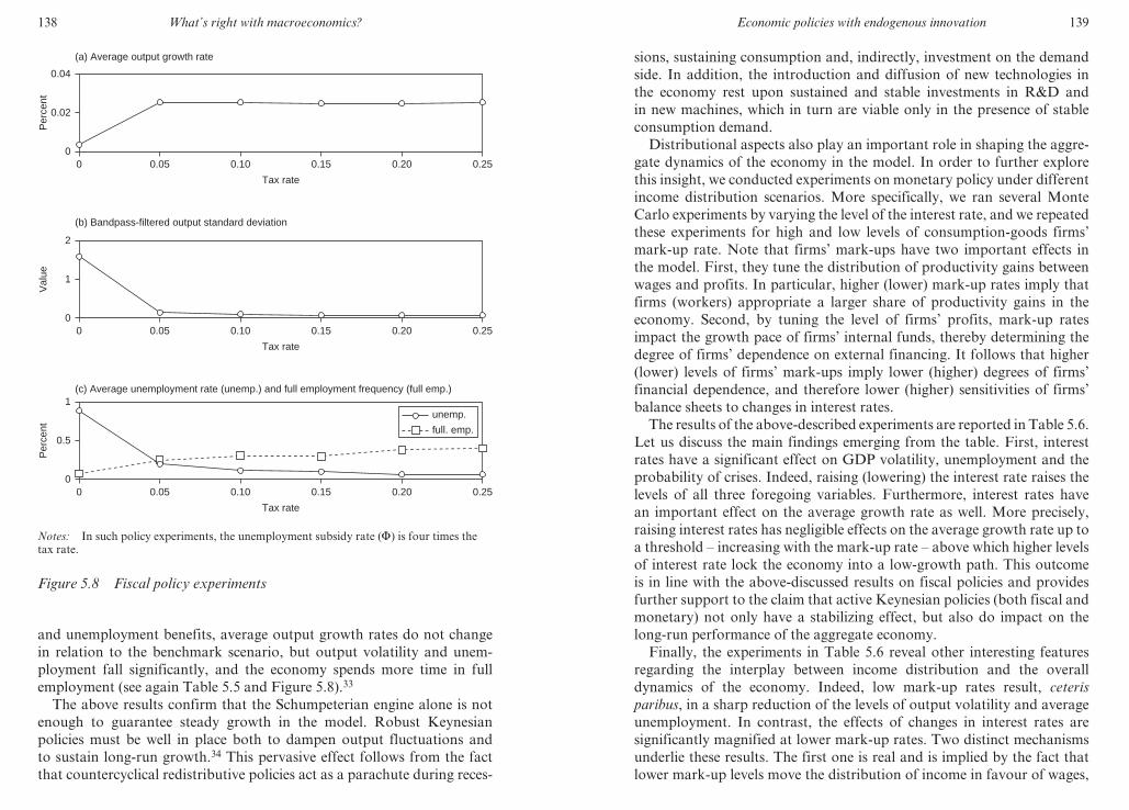
138 What’s right with macroeconomics?
and unemployment benefits, average output growth rates do not change
in relation to the benchmark scenario, but output volatility and unem-
ployment fall significantly, and the economy spends more time in full
employment (see again Table 5.5 and Figure 5.8).33
The above results confirm that the Schumpeterian engine alone is not
enough to guarantee steady growth in the model. Robust Keynesian
policies must be well in place both to dampen output fluctuations and
to sustain long- run growth.34 This pervasive effect follows from the fact
that countercyclical redistributive policies act as a parachute during reces-
00
0.02
0.04
0.05 0.10 0.15 0.20 0.25
Per
cent
Tax rate
(a) Average output growth rate
00
1
2
0.05 0.10 0.15 0.20 0.25
Val
ue
Tax rate
(b) Bandpass-filtered output standard deviation
00
0.5
1
0.05 0.10 0.15 0.20 0.25
Per
cent
Tax rate
unemp.full. emp.
(c) Average unemployment rate (unemp.) and full employment frequency (full emp.)
Notes: In such policy experiments, the unemployment subsidy rate (F) is four times the
tax rate.
Figure 5.8 Fiscal policy experiments
M3014 - SOLOW TEXT.indd 138 21/11/2012 13:03
Economic policies with endogenous innovation 139
sions, sustaining consumption and, indirectly, investment on the demand
side. In addition, the introduction and diffusion of new technologies in
the economy rest upon sustained and stable investments in R&D and
in new machines, which in turn are viable only in the presence of stable
consumption demand.
Distributional aspects also play an important role in shaping the aggre-
gate dynamics of the economy in the model. In order to further explore
this insight, we conducted experiments on monetary policy under different
income distribution scenarios. More specifically, we ran several Monte
Carlo experiments by varying the level of the interest rate, and we repeated
these experiments for high and low levels of consumption- goods firms’
mark- up rate. Note that firms’ mark- ups have two important effects in
the model. First, they tune the distribution of productivity gains between
wages and profits. In particular, higher (lower) mark- up rates imply that
firms (workers) appropriate a larger share of productivity gains in the
economy. Second, by tuning the level of firms’ profits, mark- up rates
impact the growth pace of firms’ internal funds, thereby determining the
degree of firms’ dependence on external financing. It follows that higher
(lower) levels of firms’ mark- ups imply lower (higher) degrees of firms’
financial dependence, and therefore lower (higher) sensitivities of firms’
balance sheets to changes in interest rates.
The results of the above- described experiments are reported in Table 5.6.
Let us discuss the main findings emerging from the table. First, interest
rates have a significant effect on GDP volatility, unemployment and the
probability of crises. Indeed, raising (lowering) the interest rate raises the
levels of all three foregoing variables. Furthermore, interest rates have
an important effect on the average growth rate as well. More precisely,
raising interest rates has negligible effects on the average growth rate up to
a threshold – increasing with the mark- up rate – above which higher levels
of interest rate lock the economy into a low- growth path. This outcome
is in line with the above- discussed results on fiscal policies and provides
further support to the claim that active Keynesian policies (both fiscal and
monetary) not only have a stabilizing effect, but also do impact on the
long- run performance of the aggregate economy.
Finally, the experiments in Table 5.6 reveal other interesting features
regarding the interplay between income distribution and the overall
dynamics of the economy. Indeed, low mark- up rates result, ceteris
paribus, in a sharp reduction of the levels of output volatility and average
unemployment. In contrast, the effects of changes in interest rates are
significantly magnified at lower mark- up rates. Two distinct mechanisms
underlie these results. The first one is real and is implied by the fact that
lower mark- up levels move the distribution of income in favour of wages,
M3014 - SOLOW TEXT.indd 139 21/11/2012 13:03

140 What’s right with macroeconomics?
thus stabilizing consumption dynamics (redistributive effect). The second
mechanism is financial and displays its effect via the higher financial
dependence of firms implied by low mark- up levels (financial dependence
effect, see above). These results also militate in favour of the conjecture
(see Kaldor, 1955, and more recently Fitoussi and Saraceno, 2010) that
more equal economies are also those characterized by milder fluctuations
and by a lower occurrence of crises. Finally, they hint at the fact that
monetary policies are much more effective in regimes characterized by low
income inequality.
CONCLUDING REMARKS
In this chapter, we have studied the properties of an agent- based model
that bridges Schumpeterian theories of technology- driven economic
growth with Keynesian theories of demand generation.
The model is characterized by the presence of both a real and a banking
sector. On the real side, the model entails the explicit account of search
and investment decisions by populations of firms that are heterogene-
ous in the technologies they master and, possibly, in their decision rules.
Aggregate macro properties emerge from the thread of interactions among
Table 5.6 Effects of interest rate for different mark- up rates
Description Avg. GDP
Growth
GDP Std.
Dev. (bpf)
Avg.
Unempl.
Prob. of large neg.
growth (< −3%)
High Mark- Up
r=0.00001 0.0277 0.0749 0.0382 0.1618
r=0.05 0.0277 0.0739 0.0435 0.1488
r=0.1 0.0277 0.0760 0.0538 0.1431
r=0.15 0.0288 0.0777 0.0488 0.2102
r=0.2 0.0291 0.0898 0.0604 0.2799
r=0.35 0.0250 0.2056 0.1333 0.3699
r=0.4 0.0144 0.3633 0.3549 0.3878
Low Mark- Up
r=0.00001 0.0274 0.0541 0.0191 0.1012
r=0.05 0.0281 0.0469 0.0145 0.0908
r=0.1 0.0290 0.0505 0.0180 0.1329
r=0.15 0.0298 0.0623 0.0217 0.2439
r=0.2 0.0288 0.1460 0.0586 0.3885
r=0.35 0.0099 0.4164 0.4546 0.4482
r=0.4 0.0010 0.4268 0.6346 0.4711
M3014 - SOLOW TEXT.indd 140 21/11/2012 13:03
Economic policies with endogenous innovation 141
economic agents, without any ex ante consistency requirements amongst
their expectations and actions. In that sense, the model may be considered
as an exercise in general disequilibrium analysis. Firms in the model endog-
enously generate new technologies – embodied in new types of ‘machines’
– via expensive and mistake- ridden search processes. Inventions then
diffuse via the adoption decisions of machine users. Hence, agents gener-
ate both micro- technological shocks and micro- demand shocks, which
together propagate through the economy. The linchpin between these two
engines is represented by the credit provided by the banking sector. The
bank employs firms’ savings to finance firms’ production and investment
activities according to a credit multiplier rule.
A central question that we address in this chapter is whether the
‘Schumpeterian engine’ by itself is able to maintain the economy on a
steady growth path characterized by full employment. We find that this is
not the case: the endogenous innovation engine is able to do that only in
the presence of a ‘Keynesian’ demand- generating engine, captured in the
model by fiscal and monetary policies.
Our results cast serious doubts on the traditional dichotomy between
variables affecting long- run growth (typically, technology- related changes)
and variables impacting short- run business fluctuations (traditional
demand- related variables). First, we find that technological innovations
appear to exert their effects at all frequencies. Second, Keynesian demand-
management policies not only contribute to reducing output volatility
and unemployment rates, but, for a large set of parameterizations, they
also affect long- run growth rates in so far as they contribute to ‘releasing’
the economy from the stagnant growth trajectory, which is indeed one of
the possible emergent meta- stable states. Finally, our results indicate that
bank credit and monetary policies can heavily affect business cycle dynam-
ics by amplifying micro- level shocks. In this respect, our results point to
the diverse effects of monetary policy in the presence of different income
distributions between profits and wages.
In the future, we plan to further exploit the flexibility and modularity
of our agent- based model to study new policy experiments under different
institutional set- ups. In particular, given the post- 2007 worldwide crisis,
an obvious direction of development is to make an in- depth study of
credit and financial markets. More specifically, we will employ the model
to assess (i) how financial crises emerge; (ii) which policies (for example,
monetary versus fiscal policies) are more suitable for coping with financial
shocks; (iii) how the regulatory framework of the banking and the finan-
cial sectors (for example, Basel- like capital requirements) can prevent
the formation of financial crises; and (iv) how the market structure of
the banking sector (for example, regional versus big national banks) can
M3014 - SOLOW TEXT.indd 141 21/11/2012 13:03

142 What’s right with macroeconomics?
amplify or dampen the effects of financial shocks. To explore the last
point, we will introduce heterogeneous banks into the model, taking into
account the emerging credit network structure between them and between
banks and firms.
NOTES
1. Thanks to Willi Semmler, Robert Solow and Tania Treibich. Thanks also to the par-
ticipants of the conference, ‘What’s right with macroeconomics?’, organized by the
Cournot Centre. All usual disclaimers apply.
2. For DSGE models, see Woodford (2003) and Galí and Gertler (2007).
3. See also Dosi et al. (2006) and Dosi et al. (2008).
4. As Blanchard (2009, p. 26) puts it, ‘To caricature only slightly: a macroeconomic article
today follows strict, haiku- like, rules: it starts from a general equilibrium structure, in
which individuals maximize the expected present value of utility, firms maximize their
value, and markets clear. Then, it introduces a twist, be it an imperfection or the closing
of a particular set of markets, and works out the general equilibrium implications. It
then performs a numerical simulation, based on calibration, showing that the model
performs well. It ends with a welfare assessment.’
5. See, however, Dosi et al. (1994) for an exception. See also Dawid (2006) for an exhaus-
tive survey of agent- based models of innovation and technical change.
6. For agent- based models with both Keynesian and Schumpeterian features, see
Verspagen (2002), Ciarli et al. (2008), Saviotti and Pyka (2008), and the discussion
in Silverberg and Verspagen (2005). See also the EURACE large- scale ABM that is
aimed at capturing the main characteristics of the European economy and addressing
European- policy analyses (Dawid et al., 2008).
7. See Fagiolo et al. (2007) for a discussion and the special issue on ‘Agent- based models
for economic policy design’, Journal of Economic Behavior and Organization, 2008,
67(2), edited by Herbert Dawid and Giorgio Fagiolo. More on that in the following
section.
8. Survey data evidence summarized in Fabiani et al. (2006) show that European firms
mostly set prices according to mark- up rules.
9. In the following, we assume all capital- producing firms to be identical in their R&D
propensity. This is not too far from reality: R&D intensities are largely sector specific
and associated with the sector- wide nature of innovative opportunities and modes of
innovative search (see Pavitt, 1984; Dosi, 1988; and Klevorick et al., 1995).
10. Firms on the technological frontier, lacking anyone to imitate, obviously invest their
entire R&D budget in the search for innovations.
11. For maximum simplicity, here we use the rule Dje(t) 5 Dj(t − 1). In Dosi et al. (2006),
we check the robustness of the simulation results employing more sophisticated
expectation- formation rules. We found that increasing the computational capabilities
of firms does not significantly change either the average growth rates or the stability of
the economy. These properties still hold in the model presented here.
12. We assume that in any given period, firms’ capital growth rates cannot exceed a fixed
maximum threshold consistent with the maximum capital growth rates found in the
empirical literature on firms’ investment patterns (see, for example, Doms and Dunne,
1998).
13. This is in line with a large body of empirical analyses (see, for example, Feldstein and
Foot, 1971; Eisner, 1972; Goolsbee, 1998) showing that replacement investment is typi-
cally not proportional to the capital stock.
14. Moreover, they also scrap the machines older than h periods (with h being a positive
integer).
M3014 - SOLOW TEXT.indd 142 21/11/2012 13:03
Economic policies with endogenous innovation 143
15. Among the empirical literature investigating the presence of gestation- lag effects in
firms’ investment expenditures, see, for example, Del Boca et al. (2008).
16. If investment plans cannot be fully realized, firms give priority to capital stock expan-
sion, as compared to the substitution of old machines.
17. This is close to the spirit of ‘customer market’ models originated by the seminal work of
Edmund Phelps and Sidney Winter (1970). See also Klemperer (1995) for a survey, and
the exploration of some important macro implications by Bruce Greenwald and Joseph
Stiglitz (2003).
18. Antecedents in the same spirit are Phelps and Winter, 1970; Klemperer, 1987; Farrel
and Shapiro, 1988; see also the empirical literature on consumers’ imperfect price
knowledge surveyed in Rotemberg, 2008.
19. Recall that consumption- goods firms fix production according to their demand expec-
tations, which may differ from actual demand. If the firm produces too much, the
inventories pile up, whereas if its production is lower than demand plus inventories, its
competitiveness is reduced accordingly.
20. Strictly speaking, a canonic replicator dynamic evolves on the unit simplex with all enti-
ties having positive shares. Equation (5.13) allows shares to become virtually negative.
In that case, the firm is pronounced dead, and market shares are re- calculated accord-
ingly. This is what we mean by a ‘quasi- replicator’ dynamic. Note that an advantage of
such a formulation is that it determines simultaneously changes in market shares and
extinction events.
21. The stock of capital of a new consumption- goods firm is obtained by multiplying the
average stock of capital of the incumbents by a random draw from a Uniform distribu-
tion with support [�1, �2], 0 , �1, , �2 # 1. In the same manner, the stock of liquid
assets of an entrant is computed by multiplying the average stock of liquid assets of the
incumbents of the sector by a random variable distributed according to a Uniform with
support [�3, �4], 0 , �3, , �4 # 1.
22. More precisely, the technology of capital- goods firms is obtained by applying a coef-
ficient extracted from a Beta (a2, b2) distribution to the endogenously evolving tech-
nology frontier (Amax(t) , Bmax(t) ) , where Amax(t) and Bmax(t) are the best technology
available to incumbents.
23. For simplicity, we assume in the following that Dw (t)
w (t 2 1) 5 DAB (t)
AB (t 2 1). Simulation results
are robust to wage dynamics involving adjustment to inflation and unemployment. For
more detailed modelling of the labour market in an evolutionary/ACE framework, see,
for example, Tesfatsion (2000) and Fagiolo et al. (2004).
24. Some methodological issues concerning the exploration of the properties of evolution-
ary/ACE models are discussed in, for example, Lane (1993); Pyka and Fagiolo (2007);
Fagiolo et al. (2007); Fagiolo and Roventini (2012).
25. Preliminary exercises confirm that, for the majority of statistics under study, Monte
Carlo distributions are sufficiently symmetric and unimodal to justify the use of across-
run averages as meaningful synthetic indicators.
26. The average growth rate of variable X (for example, GDP) is simply defined as:
GRX 5logX (T) 2 logX (0)
T 1 1,
where T 5 600 is the econometric sample size. This value for T is a conservative choice,
as the first iterative moments of growth statistics converge to a stable behaviour well
before such a time horizon. This means that the model reaches a relatively (meta) stable
behaviour soon after simulations start. Our experiment shows that choosing larger
values for T does not alter the main economic implications resulting from the simula-
tion of the model.
27. In addition, aggregate growth rates of output display fat- tailed distributions (not
shown) that are well in tune with the empirical evidence (see Castaldi and Dosi, 2008;
Fagiolo et al., 2008). Informally, that means that both in our model and in reality,
M3014 - SOLOW TEXT.indd 143 21/11/2012 13:03

144 What’s right with macroeconomics?
relatively big ‘spurs of growth’ and recessions occur much more frequently than might
be predicted on the grounds of normally distributed shocks (see also the discussion on
firm growth patterns below).
28. Interestingly, many statistical regularities concerning the structure of the economy (for
example, size distributions, fatness of firms’ growth rates, and so on) appear to hold
across an ample parameter range, under positive technological progress, even when
policies undergo the changes we study in the following section.
29. The full list of parameters under different policy scenarios is available from the authors
on request.
30. In fact, given the increasing availability of micro data, one can start thinking of disag-
gregated empirical proxies for our variables. The issue is well beyond the scope of this
chapter, however.
31. On purpose, we did not introduce any feedback between changes in IPR regimes and
propensities to search.
32. The thrust of our results on policies affecting entry, competition, and variety preserva-
tion are indeed broadly in tune with the advocacy for ‘evolutionary technology policies’
in Metcalfe (1994b), while it runs against the so- called ‘Schumpeterian hypothesis’,
according to which degrees of industrial concentration should be conducive to higher
rates of innovation.
33. On the long- run, growth- enhancing effects of countercyclical macroeconomic policies,
see the empirical evidence provided by Aghion and Marinescu (2007).
34. We also ran Monte Carlo experiments to check the robustness of Keynesian proper-
ties of the system to alternative institutional regimes governing the labour market
captured by the parameters affecting the wage rate (see equation (5.21)). In particular,
we allow wages to move as a (negative) function of the unemployment rate. Under
these ‘classical’ circumstances, wages may fall during recessions, inducing price cuts,
which in turn may increase output, supposedly weakening the case for Keynesian
fiscal policies. These experiments suggest, however, that the dynamics of the systems
are largely independent of how wages are determined. For more on that, see Dosi et
al. (2010).
REFERENCES
Acemoglu, D., P. Aghion and F. Zilibotti (2006), ‘Distance to frontier, selection, and economic growth’, Journal of the European Economic Association, 4, 37–74.
Aghion, P. and P. Howitt (1992), ‘A model of growth through creative destruction’, Econometrica, 60, 323–51.
Aghion, P. and P. Howitt (1998), Endogenous Growth, Cambridge: MIT Press.Aghion, P. and P. Howitt (2007), ‘Appropriate growth policy: a unifying frame-
work’, Journal of the European Economic Association, 4, 269–314.Aghion, P. and I. Marinescu (2007), ‘Cyclical budgetary policy and economic
growth: what do we learn from OECD panel data?’, in NBER Macroeconomics Annual, 22, 251–78.
Aghion, P., G. Angeletos, A. Banerjee and K. Manova (2010), ‘Volatility and growth: credit constraints and the composition of investment’, Journal of Monetary Economics, 57, 246–65.
Aghion, P., P. Askenazy, N. Berman, G. Cette and L. Eymard (2008), ‘Credit con-straints and the cyclicality of R&D investment: evidence from France’, Working Paper 2008- 26, Paris School of Economics.
Akerlof, G.A. (2002), ‘Behavioral macroeconomics and macroeconomic behavior’, American Economic Review, 92, 411–33.
M3014 - SOLOW TEXT.indd 144 21/11/2012 13:03
Economic policies with endogenous innovation 145
Akerlof, G.A. (2007), ‘The missing motivation in macroeconomics’, American Economic Review, 97, 5–36.
Akerlof, G.A. and J.L. Yellen (1985), ‘A near- rational model of the business cycles, with wage and price inertia’, Quarterly Journal of Economics, 100, 823–38.
Bartelsman, E. and M. Doms (2000), ‘Understanding productivity: lessons from longitudinal micro- data’, Journal of Economic Literature, 38, 569–94.
Bartelsman, E., S. Scarpetta and F. Schivardi (2005), ‘Comparative analysis of firm demographics and survival: evidence from micro- level sources in OECD countries’, Industrial and Corporate Change, 14, 365–91.
Baxter, M. and R. King (1999), ‘Measuring business cycles: approximate band- pass filter for economic time series’, The Review of Economics and Statistics, 81, 575–93.
Benhabib, J. and M. Spiegel (1994), ‘The role of human capital in economic development: evidence from aggregate cross- country data’, Journal of Monetary Economics, 34, 143–73.
Blanchard, O. (2009), ‘The state of macro’, Annual Review of Economics, 1, 209–28.Caballero, R.J. (1999), ‘Aggregate investment’, in J. Taylor and M. Woodford
(eds), Handbook of Macroeconomics, Amsterdam: Elsevier Science.Canova, F. (2008), ‘How much structure in empirical models?’, in T. Mills and
K. Patterson (eds), Palgrave Handbook of Econometrics Volume 2: Applied Econometrics, Basingstoke, UK and New York: Palgrave Macmillan.
Castaldi, C. and G. Dosi (2008), ‘The patterns of output growth of firms and countries: scale invariances and scale specificities’, Empirical Economics, 37(3), 475–95.
Caves, R. (1998), ‘Industrial organization and new findings on the turnover and mobility of firms’, Journal of Economic Literature, 36, 1947–82.
Ciarli, T., A. Lorentz, M. Savona and M. Valente (2008), ‘Structural change of production and consumption: a micro to macro approach to economic growth and income distribution’, LEM Papers Series 2008/08, Laboratory of Economics and Management (LEM), Sant’Anna School of Advanced Studies, Pisa, Italy.
Colander, D., P. Howitt, A.P. Kirman, A. Leijonhufvud and P. Mehrling (2008), ‘Beyond DSGE models: toward an empirically based macroeconomics’, American Economic Review, 98, 236–40.
Dawid, H. (2006), ‘Agent- based models of innovation and technological change’, in L. Tesfatsion and K. Judd (eds), Handbook of Computational Economics vol. II, Amsterdam: North- Holland.
Dawid, H., S. Gemkow, P. Harting, K. Kabus, M. Neugart and K. Wersching (2008), ‘Skills, innovation, and growth: an agent- based policy analysis’, Journal of Economics and Statistics, 228, 251–75.
Del Boca, A., M. Galeotti, C.P. Himmelberg and P. Rota (2008), ‘Investment and time to plan and build: a comparison of structures vs. equipment in a panel of Italian firms’, Journal of the European Economic Association, 6, 864–89.
Di Guilmi, C., M. Gallegati and P. Ormerod (2004), ‘Scaling invariant distribu-tions of firms’ exit in OECD countries’, Physica A: Statistical Mechanics and its Applications, 334, 267–73.
Dinopoulos, E. and P. Segerstrom (1999), ‘A Schumpeterian model of protection and relative wages’, American Economic Review, 89, 450–72.
Doms, M. and T. Dunne (1998), ‘Capital adjustment patterns in manufacturing plants’, Review of Economic Dynamics, 1, 409–29.
M3014 - SOLOW TEXT.indd 145 21/11/2012 13:03

146 What’s right with macroeconomics?
Dosi, G. (1998), ‘Sources procedures and microeconomic effects of innovation’, Journal of Economic Literature, 26, 126–71.
Dosi, G. (2007), ‘Statistical regularities in the evolution of industries. A guide through some evidence and challenges for the theory’, in F. Malerba and S. Brusoni (eds), Perspectives on Innovation, Cambridge, MA: Cambridge University Press.
Dosi, G., G. Fagiolo and A. Roventini (2006), ‘An evolutionary model of endog-enous business cycles’, Computational Economics, 27, 3–34.
Dosi, G., G. Fagiolo and A. Roventini (2008), ‘The microfoundations of business cycles: an evolutionary, multi- agent model’, Journal of Evolutionary Economics, 18, 413–32.
Dosi, G., G. Fagiolo and A. Roventini (2010), ‘Schumpeter meeting Keynes: a policy- friendly model of endogenous growth and business cycles’, Journal of Economic Dynamics and Control, 34, 1748–67.
Dosi, G., S. Fabiani, R. Aversi and M. Meacci (1994), ‘The dynamics of inter-national differentiation: a multi- country evolutionary model’, Industrial and Corporate Change, 3, 225–42.
Dosi, G., O. Marsili, L. Orsenigo and R. Salvatore (1995), ‘Learning, market selection and the evolution of industrial structures’, Small Business Economics, 7, 411–36.
Eisner, R. (1972), ‘Components of capital expenditures: replacement and mod-ernization versus expansion’, The Review of Economics and Statistics, 54, 297–305.
Fabiani, S., M. Druant, I. Hernando, C. Kwapil, B. Landau, C. Loupias, F. Martins, T. Mathä, R. Sabbatini, H. Stahl and A. Stokman (2006), ‘What firms’ surveys tell us about price- setting behavior in the euro area’, International Journal of Central Banking, 2, 3–47.
Fagiolo, G. and A. Roventini (2012), ‘On the scientific status of economic policy: a tale of alternative paradigms’, Knowledge Engineering Review, 27, 163–85.
Fagiolo, G., G. Dosi and R. Gabriele (2004), ‘Matching, bargaining, and wage setting in an evolutionary model of labor market and output dynamics’, Advances in Complex Systems, 14, 237–73.
Fagiolo, G., A. Moneta and P. Windrum (2007), ‘A critical guide to empirical validation of agent- based models in economics: methodologies, procedures, and open problems’, Computational Economics, 30, 195–226.
Fagiolo, G., M. Napoletano and A. Roventini (2008), ‘Are output growth- rate dis-tributions fat- tailed? Some evidence from OECD countries’, Journal of Applied Econometrics, 23, 639–69.
Farrel, J. and C. Shapiro (1988), ‘Dynamic competition with switching costs’, RAND Journal of Economics, 19, 123–37.
Feldstein, M. and D. Foot (1971), ‘The other half of gross investment: replacement and modernization expenditures’, The Review of Economics and Statistics, 53, 49–58.
Fitoussi, J. and F. Saraceno (2010), ‘Inequality and macroeconomic performance’, OFCE Working Paper.
Fogel, K., R. Morck and B. Yeung (2008), ‘Big business stability and economic growth: is what’s good for General Motors good for America?’, Journal of Financial Economics, 89(1), 83–108.
Fujiwara, Y. (2004), ‘Zipf law in firms bankruptcy’, Physica A: Statistical and Theoretical Physics, 337(1–2), 219–30.
M3014 - SOLOW TEXT.indd 146 21/11/2012 13:03
Economic policies with endogenous innovation 147
Fukac, M. and A. Pagan (2006), ‘Issues in adopting DSGE models for use in the policy process’, Working Paper 10/2006, CAMA.
Galí, J. and M. Gertler (2007), ‘Macroeconomic modelling for monetary policy evaluation’, Journal of Economic Perspectives, 21, 25–46.
Goolsbee, A. (1998), ‘The business cycle, financial performance, and the retire-ment of capital goods’, NBER Working Paper 6392, Cambridge, MA: NBER.
Gourio, F. and A.K. Kashyap (2007), ‘Investment spikes: new facts and a general equilibrium exploration’, Journal of Monetary Economics, 54, 1–22.
Greenwald, B. and J. Stiglitz (1993a), ‘Financial market imperfections and busi-ness cycles’, Quarterly Journal of Economics, 108, 77–114.
Greenwald, B. and J. Stiglitz (1993b), ‘New and old Keynesians’, Journal of Economic Perspectives, 7, 23–44.
Greenwald, B. and J. Stiglitz (2003), ‘Macroeconomic fluctuations in an economy of Phelps–Winter markets’, in P. Aghion, R. Frydman, J. Stiglitz and M. Woodford (eds), Knowledge, Information, and Expectations in Modern Macroeconomics: In Honor of Edmund S. Phelps, Princeton, NJ: Princeton University Press.
Hicks, J.R. (1937), ‘Mr. Keynes and the “classics”: a suggested interpretation’, Econometrica, 5, 147–59.
Hubbard, G.R. (1998), ‘Capital- market imperfections and investment’, Journal of Economic Literature, 36, 193–225.
Kaldor, N. (1955), ‘Alternative theories of distribution’, The Review of Economic Studies, 23, 83–100.
Kirman, A.P. (2010), ‘The economic crisis is a crisis for economic theory’, CESifo Economic Studies, 56, 498–535.
Klemperer, P.D. (1987), ‘Markets with customer switching costs’, Quarterly Journal of Economics, 102, 375–94.
Klemperer, P.D. (1995), ‘Competition when consumers have switching costs: an overview with applications to industrial organization, macroeconomics and international trade’, Review of Economic Studies, 62, 515–39.
Klevorick, A.K., R. Levin, R.R. Nelson and S.G. Winter (1995), ‘On the sources and significance of interindustry differences in technological opportunities’, Research Policy, 24, 185–205.
Lane, D.A. (1993), ‘Artificial worlds and economics, part I and II’, Journal of Evolutionary Economics, 3, 89–107, 177–97.
LeBaron, B. and L. Tesfatsion (2008), ‘Modeling macroeconomies as open- ended dynamic systems of interacting agents’, American Economic Review, 98, 246–50.
Malerba, F. and L. Orsenigo (1995), ‘Schumpeterian patterns of innovation’, Cambridge Journal of Economics, 19, 47–65.
Metcalfe, J.S. (1994a), ‘Competition, Fisher’s principle and increasing returns to selection’, Journal of Evolutionary Economics, 4, 327–46.
Metcalfe, J.S. (1994b), ‘Evolutionary economics and technology policy’, The Economic Journal, 104, 932–44.
Minsky, H. (1986), Stabilizing an Unstable Economy, New Haven, CT: Yale University Press.
Napoletano, M., A. Roventini and S. Sapio (2006), ‘Are business cycles all alike? A bandpass filter analysis of the Italian and US cycles’, Rivista Italiana degli Economisti, 1, 87–118.
Nelson, R.R. and E.S. Phelps (1966), ‘Investment in humans, technological diffusion, and economic growth’, American Economic Review, 61, 69–75.
M3014 - SOLOW TEXT.indd 147 21/11/2012 13:03

148 What’s right with macroeconomics?
Nelson, R.R. and S.G. Winter (1982), An Evolutionary Theory of Economic Change, Cambridge: The Belknap Press of Harvard University Press.
Pavitt, K. (1984), ‘Sectoral patterns of technical change: towards a taxonomy and a theory’, Research Policy, 13, 343–73.
Phelps, E.S. and S.G. Winter (1970), ‘Optimal price policy under atomistic com-petition’, in E.S. Phelps (ed.), Microeconomic Foundations of Employment and Inflation Theory, New York: W.W. Norton.
Pyka, A. and G. Fagiolo (2007), ‘Agent- based modelling: a methodology for neo- Schumpeterian economics’, in H. Hanusch and A. Pyka (eds), The Elgar Companion to Neo- Schumpeterian Economics, Cheltenham, UK and Northampton, MA, USA: Edward Elgar Publishing.
Romer, P. (1990), ‘Endogenous technical change’, Journal of Political Economy, 98, 71–102.
Rotemberg, J. (2008), ‘Behavioral aspects of price setting, and their policy implica-tions’, NBER Working Paper 13754, Cambridge, MA: NBER.
Rotemberg, J. and M. Woodford (1999), ‘The cyclical behavior of prices and costs’, in J. Taylor and M. Woodford (eds), Handbook of Macroeconomics, Amsterdam: Elsevier Science.
Saviotti, P. and A. Pyka (2008), ‘Product variety, competition and economic growth’, Journal of Evolutionary Economics, 18, 323–47.
Silverberg, G. and B. Verspagen (2005), ‘Evolutionary theorizing on economic growth’, in K. Dopfer (ed.), Evolutionary Principles of Economics, Cambridge: Cambridge University Press.
Silverberg, G., G. Dosi and L. Orsenigo (1988), ‘Innovation, diversity and diffu-sion: a self- organization model’, The Economic Journal, 98, 1032–54.
Solow, R.M. (1956), ‘A contribution to the theory of economic growth’, Quarterly Journal of Economics, 70, 65–94.
Solow, R.M. (2008), ‘The state of macroeconomics’, Journal of Economic Perspectives, 22, 243–46.
Stiglitz, J. (1994), ‘Endogenous growth and cycles’, in Y. Shionoya and M. Perlman (eds), Innovation in Technology, Industries, and Institutions. Studies in Schumpeterian Perspectives, Ann Arbor, MI: The University of Michigan Press.
Stiglitz, J. and A. Weiss (1992), ‘Credit rationing in markets with imperfect infor-mation’, American Economic Review, 71, 393–410.
Stock, J. and M. Watson (1999), ‘Business cycle fluctuations in US macroeconomic time series’, in J. Taylor and M. Woodford (eds), Handbook of Macroeconomics, Amsterdam: Elsevier Science.
Tesfatsion, L. (2000), ‘Structure, behavior, and market power in an evolutionary labor market with adaptive search’, Journal of Economic Dynamics & Control, 25, 419–57.
Tesfatsion, L. and K. Judd (eds) (2006), Handbook of Computational Economics II: Agent- Based Computational Economics, Amsterdam: North Holland.
Verspagen, B. (2002), ‘Evolutionary macroeconomics: a synthesis between neo- Schumpeterian and Post- Keynesian lines of thought’, The Electronic Journal of Evolutionary Modeling and Economic Dynamics, 1007, available at: www.e- jemed.org/1007/index.php (accessed 20 June 2011).
Woodford, M. (2003), Interest and Prices: Foundations of a Theory of Monetary Policy, Princeton, NJ: Princeton University Press.
M3014 - SOLOW TEXT.indd 148 21/11/2012 13:03
149
6. Booms and busts: New Keynesian and behavioural explanations
Paul De Grauwe
INTRODUCTION
Capitalism is characterized by booms and busts, by periods of strong
growth in output followed by periods of declines in economic growth.
Every macroeconomic theory should attempt to explain these endemic
business cycle movements. How does the New Keynesian (dynamic sto-
chastic general equilibrium – DSGE) model explain booms and busts
in economic activity? And how does an alternative, behavioural model
explain these features? These are the questions analysed in this chapter.
In order to answer such questions, it is useful to present some stylized
facts about the cyclical movements of output. Figure 6.1 shows the move-
ments of the output gap in the USA since 1960. We observe strong cyclical
movements. They imply that there is strong autocorrelation in the output
–0.1
–0.05
0
0.05
0.1
1960
Q1
1962
Q3
1965
Q1
1967
Q3
1970
Q1
1972
Q3
1975
Q1
1977
Q3
1980
Q1
1982
Q3
1985
Q1
1987
Q3
1990
Q1
1992
Q3
1995
Q1
1997
Q3
2000
Q1
2002
Q3
2005
Q1
2007
Q3
Source: US Department of Commerce and Congressional Budget Office.
Figure 6.1 Output gap for the USA, 1960–2008
M3014 - SOLOW TEXT.indd 149 21/11/2012 13:03

150 What’s right with macroeconomics?
gap numbers, that is, the output gap in period t is strongly correlated with
the output gap in period t−1. The intuition is that if there are cyclical
movements, we will observe clustering of good and bad times. A posi-
tive (negative) output gap is likely to be followed by a positive (negative)
output gap in the next period. That is what we find for the US output gap
over the period 1960–2009: the autocorrelation coefficient is 0.94. Similar
autocorrelation coefficients are found in other countries.
A second stylized fact about the movements in the output gap is that
these are not normally distributed. The evidence for the USA is presented
in Figure 6.2. We find, first, that there is excess kurtosis (kurtosis 5 3.61),
which means that there is too much concentration of observations around
the mean to be consistent with a normal distribution. Second, we find that
there are fat tails, that is, there are more large movements in the output
gap than is compatible with the normal distribution. That also means
that if we were basing our forecasts on the normal distribution, we would
underestimate the probability that in any one period a large increase or
decrease in the output gap can occur. Finally, the Jarque–Bera test leads
to a formal rejection of normality of the movements in the US output gap
series.
0
2
4
6
8
10
12
14
16
18
20
–0.08 –0.06 –0.04 –0.02 0 0.02 0.04 0.06
Notes: Kurtosis: 3.61; Jarque–Bera: 7.17 with p- value = 0.027.
Source: US Department of Commerce and Congressional Budget Office.
Figure 6.2 Frequency distribution of US output gap (1960–2009)
M3014 - SOLOW TEXT.indd 150 21/11/2012 13:03
Booms and busts: New Keynesian and behavioural explanations 151
In this chapter I will contrast the rational expectations (DSGE) model
with a behavioural macroeconomic model, that is, a model in which agents
have cognitive limitations and do not understand the whole picture (the
underlying model). I will ask the question of how these two models explain
these empirical regularities.
The rational expectations model will be the New Keynesian model. Its
characteristic features are price and wage inertia. It is sufficiently well
known as not to require much explanation. The behavioural model is less
well known, and I will spend more time developing it. Its basic assumption
is that agents have cognitive limitations; in other words, they only under-
stand small bits and pieces of the whole model and use simple rules to
guide their behaviour. I will introduce rationality in the model through a
selection mechanism in which agents evaluate the performance of the rule
they are following and decide to switch or to stick to the rule depending on
how well the rule performs relative to other rules.
The modelling approach presented in this chapter is not the only pos-
sible one for modelling agents’ behaviour under imperfect information. In
fact, a large body of literature has emerged attempting to introduce imper-
fect information into macroeconomic models. These attempts have been
based mainly on the statistical learning approach pioneered by Thomas
Sargent (1993) and George Evans and Seppo Honkapohja (2001). This
literature leads to important new insights (see, for example, Gaspar et al.,
2006; Orphanides and Williams, 2004; Milani, 2007; Branch and Evans,
2009). Nevertheless, I feel that this approach still loads individual agents
with too many cognitive skills, which they probably do not possess in the
real world.1
The purpose of this chapter is to contrast the dynamics of the DSGE
model with the behavioural model, and to draw some policy conclusions.
It is very much inspired by the new literature on ‘agent- based macroeco-
nomic models’ (see Howitt, 2008; Tesfatsion, 2006, among others). The
next section presents the behavioural model. The sections that follow it
discuss the different implications that the behavioural model has when
contrasted with the rational expectations model. The last section presents
some empirical evidence, followed by the conclusion with a discussion of
some methodological issues.
A BEHAVIOURAL MACROECONOMIC MODEL
In this section, the modelling strategy is described by presenting a
standard aggregate- demand–aggregate- supply model augmented with a
Taylor rule. The novel feature of the model is that agents use simple
M3014 - SOLOW TEXT.indd 151 21/11/2012 13:03

152 What’s right with macroeconomics?
rules – heuristics – to forecast the future. These rules are subjected to an
adaptive learning mechanism, that is, agents endogenously select the fore-
casting rules that have delivered the highest performance (‘fitness’) in the
past. This selection mechanism acts as a disciplining device on the kind of
rules that are acceptable. Since agents use different heuristics, we obtain
heterogeneity. This, as will be shown, creates endogenous business cycles.
This behavioural model is contrasted with a similar model that incor-
porates rational expectations, and that is interpreted as a stylized version
of DSGE models. This comparison will make it possible to focus on
some crucial differences in the transmission of shocks, in particular, of
monetary policy shocks.
The Model
The model consists of an aggregate demand equation, an aggregate supply
equation and a Taylor rule.
The aggregate demand equation is specified in the standard way, that is:
yt 5 a1E|
tyt11 1 (1 2 a1)yt21 1 a2
(rt 2 E|
tpt11) 1 et (6.1)
where yt is the output gap in period t, rt the nominal interest rate, pt the
rate of inflation, and et a white noise disturbance term. E|
t is the expecta-
tions operator where the tilde above E refers to expectations that are not
formed rationally. This process will be specified subsequently. I follow the
procedure introduced in DSGE models of adding a lagged output to the
demand equation. This is usually justified by invoking habit formation.
I keep this assumption here as I want to compare the behavioural model
with the DSGE rational expectations model. I will show later, however,
that I do not really need this inertia- building device to generate inertia in
the endogenous variables.
The aggregate supply equation can be derived from profit maximization
of individual producers. As in DSGE models, a Calvo pricing rule and
some indexation rule used in adjusting prices are assumed. This leads to
a lagged inflation variable in the equation.2 The supply curve can also be
interpreted as a New Keynesian Philips curve:
pt 5 b1E|
tpt11 1 (1 2 b1)pt21 1 b2yt 1 ht (6.2)
Finally, the Taylor rule describes the behaviour of the central bank:
rt 5 c1(pt 2 p*) 1 c2yt 1 c3rt21 1 ut (6.3)
M3014 - SOLOW TEXT.indd 152 21/11/2012 13:03
Booms and busts: New Keynesian and behavioural explanations 153
where p* is the inflation target, which for the sake of convenience will be
set equal to 0. Note that, as is commonly done, the central bank is assumed
to smooth the interest rate. This smoothing behaviour is represented by
the lagged interest rate in equation (6.3). Ideally, the Taylor rule should
be formulated using a forward- looking inflation variable, that is, central
banks set the interest rate on the basis of their forecasts about the rate of
inflation. This was not done here in order to maintain simplicity in the
model.
Introducing heuristics in the forecasting output
Agents are assumed to use simple rules (heuristics) to forecast the future
output and inflation. I proceed as follows. I start with a very simple fore-
casting heuristics and apply it to the forecasting rules of future output. I
assume two types of forecasting rules. The first rule can be called ‘funda-
mentalist’. Agents estimate the steady- state value of the output gap (which
is normalized at 0) and use this to forecast the future output gap. (In a
later extension, it will be assumed that agents do not know the steady-
state output gap with certainty and only have biased estimates of it.) The
second forecasting rule is an ‘extrapolative’ one. It does not presuppose
that agents know the steady- state output gap; they are agnostic about it.
Instead, agents extrapolate the previously observed output gap into the
future.
The two rules are specified as follows: the fundamentalist rule is defined
by:
E| f
tyt11 5 0 (6.4)
The extrapolative rule is defined by:
E|e
tyt11 5 yt21 (6.5)
This kind of simple heuristic has often been used in the behavioural
finance literature where agents are assumed to use fundamentalist and
chartist rules (see Brock and Hommes, 1997; Branch and Evans, 2006; De
Grauwe and Grimaldi, 2006). It is probably the simplest possible assump-
tion one can make about how agents, who experience cognitive limita-
tions, use rules that embody limited knowledge to guide their behaviour.
In this sense, they are bottom- up rules. They only require agents to use
information they understand, and do not require them to understand the
whole picture.
Thus, the specification of the heuristics in (6.4) and (6.5) should not be
interpreted as a realistic representation of how agents forecast. Rather, it
M3014 - SOLOW TEXT.indd 153 21/11/2012 13:03

154 What’s right with macroeconomics?
is a parsimonious representation of a world where agents do not know the
‘Truth’ (that is, the underlying model). The use of simple rules does not
mean that the agents are dumb and that they do not want to learn from
their errors. I will specify a learning mechanism later in this section in
which these agents continuously try to correct for their errors by switching
from one rule to the other.
The market forecast is obtained as a weighted average of these two
forecasts, that is:
E|
tyt11 5 af,t E|f
tyt11 1 ac,t E|e
tyt11 (6.6)
E|
tyt11 5 af,t0 1 ac,tyt21 (6.7)
and
af,t 1 ae,t 5 1 (6.8)
where af,t and ae,t are the probabilities that agents use a fundamentalist or
an extrapolative rule, respectively.
A methodological issue arises here. The forecasting rules (heuristics)
introduced are not derived at the micro level and then aggregated. Instead,
they are imposed ex post on the demand and supply equations. This has
also been the approach in the learning literature pioneered by Evans and
Honkapohja (2001). One could argue, therefore, that my modelling tech-
nique is still not fully bottom- up. Ideally one would like to derive the heu-
ristics from the micro level in an environment in which agents experience
cognitive problems. Our knowledge about how to model this behaviour at
the micro level and how to aggregate it is too sketchy, however, so I have
not tried to do so.3 Clearly, this is an area that will have to be researched
in the future.
As indicated earlier, agents are rational in the sense that they continu-
ously evaluate their forecasting performance. I apply notions of discrete
choice theory (see Anderson et al., 1992; and Brock and Hommes, 1997)
in specifying the procedure agents follow in this evaluation process.
Discrete choice theory analyses how agents decide between differ-
ent alternatives. The theory takes the view that agents are boundedly
rational, that is, utility has a deterministic component and a random
component. Agents compute the forecast performance of the different
heuristics as follows:
Uf, t 5 2 a`
k50
wk[yt2k21 2 E
|f,t2k22 yt2k21
]2 (6.9)
M3014 - SOLOW TEXT.indd 154 21/11/2012 13:03
Booms and busts: New Keynesian and behavioural explanations 155
Ue,t 5 2 a`
k50
wk[yt2k21 2 E
|e, t2k22 yt2k21
]2 (6.10)
where Uf,t and Ue,t are the forecast performances (utilities) of the funda-
mentalists and extrapolators, respectively. These are defined as the mean
squared forecasting errors (MSFEs) of the optimistic and pessimistic fore-
casting rules; wk are geometrically declining weights.
Applying discrete choice theory, the probability that an agent will use
the fundamentalist forecasting rule is given by the expression (Anderson et
al., 1992; Brock and Hommes, 1997):
af,t 5exp(gUf,t
)
exp(gUf,t) 1 exp(gUe,t
) (6.11)
Similarly the probability that an agent will use the extrapolative fore-
casting rule is given by:
ae,t 5exp(gUe,t
)
exp(gUf,t) 1 exp(gUe,t
)5 1 2 af,t (6.12)
Equation (6.11) says that as the past forecasting performance of the
fundamentalists improves relative to that of the extrapolators, agents are
more likely to select the fundamentalist rule about the output gap for their
future forecasts. As a result, the probability that agents will use the funda-
mentalist rule increases. Equation (6.12) has a similar interpretation. The
parameter g measures the ‘intensity of choice’. It parametrizes the extent
to which the deterministic component of utility determines actual choice.
When g 5 0, utility is purely stochastic. In that case, agents decide to be
fundamentalist or extrapolator by tossing a coin, and the probability to be
fundamentalist (or extrapolator) is exactly 0.5. When g 5 ∞, utility is fully
deterministic and the probability of using a fundamentalist rule is either 1
or 0. The parameter g can also be interpreted as expressing a willingness
to learn from past performance. When g 5 0, this willingness is zero; it
increases with the size of g.
Note that this selection mechanism is the disciplining device introduced
in this model on the kind of rules of behaviour that are acceptable. Only
those rules that pass the fitness test remain in place. The others are weeded
out. In contrast with the disciplining device implicit in rational expecta-
tions models, implying that agents have superior cognitive capacities, we
do not have to make such an assumption here.
It should also be stressed that although individuals use simple rules in
forecasting the future, this does not mean that they fail to learn. In fact,
M3014 - SOLOW TEXT.indd 155 21/11/2012 13:03

156 What’s right with macroeconomics?
the fitness criterion used should be interpreted as a learning mechanism
based on ‘trial and error’. When observing that the rule they use performs
less well than the alternative rule, agents are willing to switch to the better
performing rule. Put differently, agents avoid making systematic mistakes
by constantly being willing to learn from past mistakes and to change their
behaviour. This also ensures that the market forecasts are unbiased.
The mechanism driving the selection of the rules introduces a self-
organizing dynamic into the model. This dynamic goes beyond the capac-
ity of understanding of any one individual in the model. In this sense it
is a bottom- up system. It contrasts with the mainstream macroeconomic
models in which it is assumed that some or all agents can take a bird’s
eye view and understand the whole picture. These agents not only under-
stand the whole picture, but also use this whole picture to decide on their
optimal behaviour. Thus, there is a one- to- one correspondence between
the total information embedded in the world and the individuals’ brains.
Introducing heuristics in forecasting inflation
Agents also have to forecast inflation. A similar simple heuristics is used
as in the case of output gap forecasting, with one rule that could be called
a fundamentalist rule and the other an extrapolative rule (see Brazier et
al., 2006, for a similar set- up). The fundamentalist rule is based on the
announced inflation target, that is, agents using this rule have confidence
in its credibility and use it to forecast inflation. The extrapolative rule is
used by agents who do not trust the announced inflation target. Instead
they extrapolate inflation from the past into the future.
The fundamentalist rule will be called an ‘inflation targeting’ rule. It
consists in using the central bank’s inflation target to forecast future infla-
tion, such that:
E|tar
t 5 p* (6.13)
where the inflation target p* is normalized to be equal to 0.
The ‘extrapolators’ are defined by:
E|ext
t pt11 5 pt21 (6.14)
The market forecast is a weighted average of these two forecasts, such
that:
E|
tpt11 5 btar,t E|tar
t pt11 1 bext,tE|ext
t pt11 (6.15)
or
M3014 - SOLOW TEXT.indd 156 21/11/2012 13:03
Booms and busts: New Keynesian and behavioural explanations 157
E|
tpt11 5 btar,tp* 1 bext,tpt21 (6.16)
and
btar,t 1 bext,t 5 1 (6.17)
The same selection mechanism is used as in the case of output forecasting
to determine the probabilities of agents who trust the inflation target and
those who do not and revert to extrapolation of past inflation, such that:
btar,t 5exp(gUtar,t
)
exp(gUtar,t) 1 exp(gUext,t
) (6.18)
bext,t 5exp(gUext,t
)
exp(gUtar,t) 1 exp(gUext,t
) (6.19)
where Utar,t and Uext,t are the weighted averages of past squared forecast
errors of using targeter and extrapolator rules, respectively. These are
defined in the same way as in (6.9) and (6.10).
This inflation forecasting heuristics can be interpreted as a procedure
of agents to find out how credible the central bank’s inflation targeting is.
If this is very credible, using the announced inflation target will produce
good forecasts, and as a result, the probability that agents will rely on the
inflation target will be high. If, on the other hand, the inflation target does
not produce good forecasts (compared to a simple extrapolation rule), the
probability that agents will use it will be small.
The solution of the model is found by first substituting (6.3) into (6.1)
and rewriting in matrix notation. This yields:
c 1 2 b2
2a2c1 1 2 a2c2
d cpt
yt
d 5 c b1 0
2a2 a1
d cE|tpt11
E|
tyt11
d 1 c1 2 b1 0
0 1 2 a1
d cpt21
yt21
d 1 c 0
a2c3
d rt21 1 c ht
a2ut1 et
dor
A Zt 5 B E|tZt11 1 C Zt21 1 b rt21 1 vt (6.20)
M3014 - SOLOW TEXT.indd 157 21/11/2012 13:03

158 What’s right with macroeconomics?
where bold characters refer to matrices and vectors. The solution for Zt is
given by
Zt 5 A21 [B E|tZt11 1 C Zt21 1 b rt21 1 vt ] (6.21)
The solution exists if the matrix A is non- singular, that is, if (1 2 a2c2)
a2b2c1 ≠ 0. The system (6.21) describes the solution for yt and pt given the
forecasts of yt and pt. The latter have been specified in equations (6.4)
to (6.12) and can be substituted into (6.21). Finally, the solution for rt is
found by substituting yt and pt obtained from (6.21) into (6.3).
My research strategy consists in comparing the dynamics of this behav-
ioural model with the same structural model (aggregate demand equation
(6.1), aggregate supply equation (6.2) and Taylor rule equation (6.3))
under rational expectations, which I interpret as a stylized DSGE- model.
The model consisting of equations (6.1) to (6.3) can be written in matrix
notation as follows:
£ 1 2 b2 0
0 1 2 a2
2c1 2 c2 1
§ £pt
yt
rt
§ 5 £ b1 0 0
2a2 a1 0
0 0 0
§ £Etpt11
Etyt11
Etrt11
§
1 £ 1 2 b1 0 0
0 1 2 a1 0
0 0 a3
§ £pt21
yt21
rt21
§ 1 £ht
et
ut
§ WZt 5 FEtZt11 1 LZt21 1 vt (6.22)
Zt 5 W21 [FEtZt11 1 LZt21 1 vt ] (6.23)
This model can be solved under rational expectations using the Binder–
Pesaran (1996) procedure.
Calibrating the Model
I proceed by calibrating the model. In the Appendix, the parameters used
in the calibration exercise are presented. The model was calibrated in such
a way that the time units can be considered to be months. A sensitivity
analysis of the main results to changes in some of the parameters of the
model will be presented. The three shocks (demand, supply and interest
rate) are independent and identically distributed (i.i.d.) with standard
deviations of 0.5 per cent.
M3014 - SOLOW TEXT.indd 158 21/11/2012 13:03
Booms and busts: New Keynesian and behavioural explanations 159
ANIMAL SPIRITS, LEARNING AND FORGETFULNESS
In this section simulations of the behavioural model in the time domain
are presented and interpreted. The upper panel of Figure 6.3 shows the
time pattern of the output gap produced by the behavioural model. A
strong cyclical movement in the output gap can be observed. The lower
panel of Figure 6.3 shows a variable called ‘animal spirits’.4 It represents
the evolution of the fractions of the agents who extrapolate a positive
output gap. Thus when the curve reaches 11, all agents are extrapolating a
positive output gap; when the curve reaches 0, no agents are extrapolating
a positive output gap. In fact, in that case they all extrapolate a negative
Output
Leve
l
4
3
2
1
0
–1
–2
–3
–41000 1050 1100 1150
Time1200 1250 1300
Animal spirits
Leve
l
00.10.20.30.40.50.60.70.80.91.0
1000 1050 1100 1150Time
1200 1250 1300
Figure 6.3 Output gap in behavioural model
M3014 - SOLOW TEXT.indd 159 21/11/2012 13:03

160 What’s right with macroeconomics?
output gap. The curve thus shows the degree of optimism and pessimism
of agents who make forecasts of the output gap.
Combining the information of the two panels in Figure 6.3, it can be
seen that the model generates endogenous waves of optimism and pessi-
mism. During some periods optimists (that is, agents who extrapolate pos-
itive output gaps) dominate, and this translates into above- average output
growth. These optimistic periods are followed by pessimistic ones when
pessimists (that is, agents who extrapolate negative output gaps) domi-
nate, and the growth rate of output is below average. These waves of opti-
mism and pessimism are essentially unpredictable. Other realizations of
the shocks produce different cycles with the same general characteristics.
These endogenously generated cycles in output are made possible by
a self- fulfilling mechanism that can be described as follows. A series of
random shocks creates the possibility that one of the two forecasting
rules – say the extrapolating one – delivers a higher pay- off, that is, a
lower mean squared forecast error (MSFE). This attracts agents that were
using the fundamentalist rule. If the successful extrapolation happens to
be a positive extrapolation, more agents will start extrapolating the posi-
tive output gap. The ‘contagion effect’ leads to an increasing use of the
optimistic extrapolation of the output gap, which in turn stimulates aggre-
gate demand. Optimism is therefore self- fulfilling. A boom is created. At
some point, negative stochastic shocks and/or the reaction of the central
bank through the Taylor rule make a dent in the MSFE of the optimistic
forecasts. Fundamentalist forecasts may become attractive again, but it
is equally possible that pessimistic extrapolation becomes attractive and
therefore fashionable again. The economy turns around.
These waves of optimism and pessimism can be understood to be
searching (learning) mechanisms of agents who do not fully understand
the underlying model but are continuously searching for the truth. An
essential characteristic of this searching mechanism is that it leads to
systematic correlation in beliefs (for example, optimistic extrapolations
or pessimistic extrapolations). This systematic correlation is at the core
of the booms and busts created in the model. Note, however, that when
computed over a significantly long period of time, the average error in the
forecasting goes to zero. In this sense, the forecast bias tends to disappear
asymptotically.
The results concerning the time path of inflation are shown in Figure 6.4.
The lower panel of Figure 6.4 shows the fraction of agents using the
extrapolator heuristics, that is, the agents who do not trust the inflation
target of the central bank. One can identify two regimes. There is a regime
in which the fraction of extrapolators fluctuates around 50 per cent, which
also implies that the fraction of forecasters using the inflation target as
M3014 - SOLOW TEXT.indd 160 21/11/2012 13:03
Booms and busts: New Keynesian and behavioural explanations 161
their guide (the ‘inflation targeters’) is around 50 per cent. This is sufficient
to maintain the rate of inflation within a narrow band of approximately 1
or −1 per cent around the central bank’s inflation target. There is a second
regime, though that occurs when the extrapolators are dominant. During
this regime, the rate of inflation fluctuates significantly more. Thus, the
inflation targeting of the central bank is fragile. It can be undermined
when forecasters decide that relying on past inflation movements produces
better forecasting performances than relying on the central bank’s infla-
tion target. This can occur unpredictably as a result of stochastic shocks
in supply and/or demand. I will return to the question of how the central
bank can reduce this loss of credibility.
The simulations reported in the previous section assumed a given set
Inflation
Leve
l
4
3
2
1
0
–1
–2
–3
–41000 1050 1100 1150
Time1200 1250 1300
Fraction extrapolators
Leve
l
0.1
0.2
0.3
0.4
0.5
0.6
0.7
0.8
0.9
1.0
1000 1050 1100 1150Time
1200 1250 1300
Figure 6.4 Inflation in behavioural model
M3014 - SOLOW TEXT.indd 161 21/11/2012 13:03

162 What’s right with macroeconomics?
of numerical values of the parameters of the model. It was found that for
this set of parameter values, animal spirits (measured by the movements
in the fraction of optimistic extrapolators) emerge and affect the fluctua-
tions of the output gap. The correlation coefficient between the fraction
of optimists and the output gap in the simulation reported in Figure 6.3
is 0.86. One would like to know how this correlation evolves when one
changes the parameter values of the model. I concentrate on two param-
eter values here: the intensity of choice parameter, g, and the memory
agents have when calculating the performance of their forecasting. The
latter is represented by the parameter wk in equations (6.9) and (6.10), and
is a series of declining weights attached to past forecasting errors. I define
wk 5 (1 2 r)rk (and 0 # r # 1). The parameter r can then be interpreted
as a measure of the memory of agents. When r 5 0, there is no memory,
meaning only last period’s performance matters in evaluating a forecast-
ing rule; when r 5 1, there is infinite memory, meaning all past errors,
however far in the past, obtain the same weight.
The results of the sensitivity analysis are shown in Figure 6.5. The left-
hand panel shows the correlation between the output gap and the fraction
of optimistic extrapolators (animal spirits) for increasing values of the
intensity of choice parameter, g. It can be seen that when g is zero (that
is, when the switching mechanism is purely stochastic), this correlation is
zero. The interpretation is that in an environment in which agents decide
purely randomly – in other words, they do not react to the performance
of their forecasting rule – there are no systematic waves of optimism and
0.1
0.2
0.3
0.4
0.5
Memory
Correlation between outputand animal spirits
0.6
0.7
0.8
0.9
1.00
0.1
0.2
0.3
0.4
0.5
0.6
0.7
0.8
0.9
1.00.
2
0.4
0.6
0.8
1.0
Intensity of choice
Cor
rela
tion
outp
ut-s
pirit
sCorrelation between output
and animal spirits
1.2
1.4
1.6
1.8
2.00
0.1
0.2
0.3
0.4
0.5
0.6
0.7
0.8
0.9
1.0
Figure 6.5 Correlations between output gap and fraction of optimists
M3014 - SOLOW TEXT.indd 162 21/11/2012 13:03
Booms and busts: New Keynesian and behavioural explanations 163
pessimism (animal spirits) that can influence the business cycle. When
g increases, the correlation increases sharply. Thus, in an environment
in which agents learn from their mistakes, animal spirits arise. One thus
needs a minimum level of rationality (in the sense of a willingness to learn)
for animal spirits to emerge and to influence the business cycle. Figure 6.3
shows that this is achieved with relatively low levels of g.
The right- hand panel shows the correlation between the output gap and
the fraction of optimists for increasing values of the memory parameter r.
It can be seen that when r 5 1 the correlation is zero. This is the case where
agents attach the same weight to all past observations, however far in the
past they occurred. Put differently, when agents have infinite memory,
they forget nothing. In that case animal spirits do not occur. Thus one
needs some forgetfulness (which is a cognitive limitation) to produce
animal spirits. Note that the degree of forgetfulness does not have to be
large. For values of r below 0.98, the correlations between output and
animal spirits are quite high.
Having presented the main features of the behavioural model, I will
now proceed to show how this model leads to a view of macroeconomic
dynamics that contrasts greatly with the one obtained from the rational-
expectations DSGE models. I will concentrate on two areas. The first
one has to do with the business cycle theories implicit in the behavioural
and the rational expectations models. The second one focuses on the
implications for monetary policies.
TWO DIFFERENT BUSINESS CYCLE THEORIES
Are the behavioural and the New Keynesian models capable of mimicking
these empirical regularities? Let us first focus on the behavioural model
presented in the previous section. Figure 6.3 presented a typical simulation
of the output gap obtained in that model. The autocorrelation coefficient
of the output gap obtained in Figure 6.3 is 0.95, which is very close to 0.94,
that is, the autocorrelation of the output gap in the USA during 1960–
2009 (see the introduction). In addition, my behavioural macroeconomic
model produces movements of output that are very different from the
normal distribution. I show this by presenting the histogram of the output
gaps obtained from Figure 6.3. The result is presented in Figure 6.6. The
frequency distribution of the output gap deviates significantly from a
normal distribution. There is excess kurtosis (kurtosis 5 4.4), meaning
there is too much concentration of observations around the mean for the
distribution to be normal. In addition, there are fat tails. This means that
there are too many observations that are extremely small or extremely
M3014 - SOLOW TEXT.indd 163 21/11/2012 13:03

164 What’s right with macroeconomics?
large to be compatible with a normal distribution. I also applied a more
formal test of normality, the Jarque–Bera test, which rejected normal-
ity. Note that the non- normality of the distribution of the output gap is
produced endogenously by the model, as I feed the model with normally
distributed shocks.
This result is not without implications. It implies that when we use the
assumption of normality in macroeconomic models, we underestimate the
probability of large changes. In this particular case, assuming normal dis-
tributions tends to underestimate the probability that intense recessions or
booms will occur. The same is true in finance models that assume normal-
ity. These models greatly underestimate the probability of extremely large
asset price changes. In other words, they underestimate the probability
of large bubbles and crashes. To use the metaphor introduced by Nassim
Taleb, there are many more Black Swans than theoretical models based on
the normality assumption.
It is fine to observe this phenomenon. It is even better to have an expla-
nation for it. My model provides such an explanation. It is based on the
particular dynamics of ‘animal spirits’, illustrated in Figure 6.7, which
shows the frequency distribution of the animal spirits index (defined
0
20
40
60
80
100
120
140
160
180
–8 –6 –4 –2 0 2 4 6 8
Histogram output gap
Notes: Kurtosis = 4.4, Jarque–Bera = 178.4 (p- value = 0.001).
Figure 6.6 Frequency distribution of simulated output gap
M3014 - SOLOW TEXT.indd 164 21/11/2012 13:03
Booms and busts: New Keynesian and behavioural explanations 165
earlier). This index is associated with the frequency distribution of the
output gap obtained in Figure 6.6. From Figure 6.7, we observe that there
is a concentration of the animal spirits at the extreme values of 0 and 1 and
also in the middle of the distribution (but more spread out). This feature
provides the key explanation of the non- normality of the movements of
the output gap.
When the animal spirits index clusters in the middle of the distribution,
we have tranquil periods. There is no particular optimism or pessimism,
and agents use a fundamentalist rule to forecast the output gap. At
irregular intervals, however, the economy is gripped by either a wave of
optimism or of pessimism. The nature of these waves is that beliefs get cor-
related. Optimism breeds optimism; pessimism breeds pessimism. This can
lead to situations where everybody has become either optimistic or pes-
simistic. These periods are characterized by extreme positive or negative
movements in the output gap (booms and busts).
From the previous discussion, it follows that my behavioural macroeco-
nomic model has a strong prediction about how the movements of the
output gap are distributed. These movements should be non- normal. This
is also what one observes in reality.
How well does the New Keynesian (DSGE) model perform in mim-
icking the empirical regularities about the business cycle? I simulated
0
50
100
150
200
250
300
350
400
450
0 0.2 0.4 0.6 0.8 1
Histogram animal spirits
Figure 6.7 Frequency distribution of simulated animal spirits
M3014 - SOLOW TEXT.indd 165 21/11/2012 13:03

166 What’s right with macroeconomics?
the Rational Expectations version of equations (6.1) to (6.3) (the New
Keynesian model) using the same calibration. I show the movements of
the simulated output gap in Figure 6.8. The upper panel shows the output
gap in the time domain and the lower panel in the frequency domain. The
autocorrelation in the output gap is 0.77, which is significantly lower than
in the observed data (for the USA, I found 0.94). In addition, these output
gap movements are normally distributed (see lower panel). We cannot
reject that the distribution is normal.
The next step in making this model more empirically relevant consists
in adding autocorrelation in the error terms. This is now the standard
procedure in DSGE models (see Smets and Wouters, 2003). I have done
the same with my version of the New Keynesian model and assumed that
the autocorrelation of the error terms in equations (6.1) to (6.3) is equal
to 0.9. The result of this assumption is shown in the simulations of the
output gap in Figure 6.9. We now obtain movements of the output gap
that resemble real- life movements. The autocorrelation of the output gap
is now 0.98, which is very close to the observed number of 0.94 in the
post- war US output gap. We still cannot reject normality though (see the
Jarque–Bera test). This is a problem that DSGE models have not been
able to solve.
Thus, in order to mimic business cycle movements, the New Keynesian
(DSGE) model builders have had recourse to introducing autocorrelation
in the error terms (the shocks that hit the economy). This trick has allowed
DSGE models to closely fit observed data (see Smets and Wouters, 2003).
This success has been limited to the first and second moments of the move-
ments of output, but not to the highest moments (kurtosis, fat tails). The
latter failure has the implication that in order to explain a large move-
ment in output (for example, a deep recession, or a strong boom), DSGE
models have to rely on large unpredictable shocks.
There are two problems with this theory of the business cycle implicit in
the DSGE models. First, business cycles are not the result of endogenous
dynamics. They occur as a result of exogenous shocks and slow transmis-
sion of those shocks. Put differently, the DSGE models picture a world
populated by rational agents who are fully informed. In such a world,
there would never be business cycles. The latter arise because of exogenous
disturbances and of constraints on agents’ ability to react instantane-
ously to these shocks. A given shock will thus produce ripple effects in the
economy, that is, cyclical movements.
The second problem is methodological. When the New Keynesian
model is tested empirically, the researcher finds that a lot of the output
dynamics are not predicted by the model. These unexplained dynamics are
then found in the error term. Everything is fine up to this point. The next
M3014 - SOLOW TEXT.indd 166 21/11/2012 13:03
Booms and busts: New Keynesian and behavioural explanations 167
Output
Leve
l
0.04
0.06
0.08
0.02
0
–0.02
–0.04
–0.06
–0.081000 1050 1100 1150
Time1200 1250 1300
0
20
40
60
80
100
120
–0.1 –0.05 0 0.05 0.1
Histogram output gap
Note: Kurtosis: 2.9; Jarque–Bera: 1.03 with p- value = 0.5.
Figure 6.8 Simulated output gap in extended New Keynesian model
M3014 - SOLOW TEXT.indd 167 21/11/2012 13:03
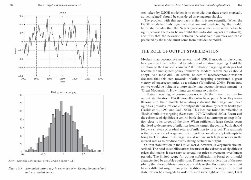
168 What’s right with macroeconomics?
0
20
40
60
80
100
140
120
–0.1 –0.5 0 0.5 1
Histogram output gap
OutputLe
vel
0.4
0.6
0.2
0
–0.2
–0.4
–0.6
–0.81000 1050 1100 1150
Time1200 1250 1300
Note: Kurtosis: 3.16; Jarque–Bera: 3.2 with p- value = 0.17.
Figure 6.9 Simulated output gap in extended New Keynesian model and
autocorrelated errors
M3014 - SOLOW TEXT.indd 168 21/11/2012 13:03
Booms and busts: New Keynesian and behavioural explanations 169
step taken by DSGE modellers is to conclude that these errors (typically
autocorrelated) should be considered as exogenous shocks.
The problem with this approach is that it is not scientific. When the
DSGE modeller finds dynamics that are not predicted by the model,
he or she decides that the New Keynesian model must nevertheless be
right (because there can be no doubt that individual agents are rational),
and thus that the deviation between the observed dynamics and those
predicted by the model must come from outside the model.
THE ROLE OF OUTPUT STABILIZATION
Modern macroeconomics in general, and DSGE models in particular,
have provided the intellectual foundation of inflation targeting. Until the
eruption of the financial crisis in 2007, inflation targeting strategies had
become the undisputed policy framework modern central banks should
adopt. And most did. The official holders of macroeconomic wisdom
declared that this step towards inflation targeting constituted a great
victory of macroeconomics as a science (Woodford, 2009). From now
on, we would be living in a more stable macroeconomic environment – a
‘Great Moderation’. How things can change so quickly.
Inflation targeting, of course, does not imply that there is no role for
output stabilization. DSGE modellers who have put a New Keynesian
flavour into their models have always stressed that wage and price
rigidities provide a rationale for output stabilization by central banks (see
Clarida et al., 1999; and Galí, 2008). This idea has found its reflection in
‘flexible’ inflation targeting (Svensson, 1997; Woodford, 2003). Because of
the existence of rigidities, a central bank should not attempt to keep infla-
tion close to its target all the time. When sufficiently large shocks occur
that lead to departures of inflation from its target, the central bank should
follow a strategy of gradual return of inflation to its target. The rationale
is that in a world of wage and price rigidities, overly abrupt attempts to
bring back inflation to its target would require such high increases in the
interest rate as to produce overly strong declines in output.
Output stabilization in the DSGE world, however, is very much circum-
scribed. The need to stabilize arises because of the existence of rigidities in
prices that makes it necessary to spread out price movements over longer
periods. The limited scope for output stabilization is based on a model
characterized by a stable equilibrium. There is no consideration of the pos-
sibility that the equilibrium may be unstable or that fluctuations in output
have a different origin than price rigidities. Should the scope for output
stabilization be enlarged? In order to shed some light on this issue, I will
M3014 - SOLOW TEXT.indd 169 21/11/2012 13:03

170 What’s right with macroeconomics?
now derive the trade- off between output and inflation variability in the
context of the behavioural model, and formulate some policy conclusions.
The trade- offs are constructed as follows. The model was simulated
10 000 times, and the average output and inflation variabilities were com-
puted for different values of the Taylor rule parameters. Figure 6.10 shows
how output variability (Panel a) and inflation variability (Panel b) change
as the output coefficient (c2) in the Taylor rule increases from 0 to 1. Each
line represents the outcome for different values of the inflation coefficient
(c1) in the Taylor rule.
Panel a, showing the evolution of output variability exhibits the
expected result: as the output coefficient (c2) increases (inflation target-
ing becomes less strict), output variability tends to decrease. One would
now expect that this decline in output variability resulting from more
active stabilization comes at the cost of more inflation variability. This,
however, is not found in Panel b. We observe that the relationship is
non- linear. As the output coefficient is increased from zero, inflation vari-
ability first declines. Only when the output coefficient increases beyond
a certain value (in a range from 0.6–0.8) does inflation variability start
to increase. Thus, the central bank can reduce both output and infla-
tion variability when it moves away from strict inflation targeting (c2 5
0) and engages in some output stabilization without overdoing it. Too
much output stabilization reverses the relationship and increases inflation
variability.
Figure 6.10 makes it possible to construct the trade- offs between output
and inflation variability. These are shown in Figure 6.11 for different
values of the inflation parameter c1. Take the trade- off AB. This is the one
obtained for c1 5 1. Start from point A on the trade- off. In point A, the
output parameter is c2 5 0 (strict inflation targeting). As output stabiliza-
tion increases, it first moves downwards. Thus, increased output stabili-
zation by the central bank reduces output and inflation variability. The
relation is non- linear, however. At some point, with an overly high output
stabilization parameter, the trade- off curve starts to increase, becoming
a ‘normal’ trade- off: a lower output variability is obtained at the cost of
increased inflation variability.
How can we interpret these results? Let us start from the case of strict
inflation targeting, that is, the authorities set c2 5 0. There is no attempt
at stabilizing output at all. The ensuing output variability intensifies the
waves of optimism and pessimism (animal spirits), which in turn feed back
into output volatility. These large waves lead to higher inflation variabil-
ity. Thus, some output stabilization is good; it reduces both output and
inflation variability by preventing overly large swings in animal spirits.
With no output stabilization at all (c2 5 0), the forces of animal spirits are
M3014 - SOLOW TEXT.indd 170 21/11/2012 13:03
Booms and busts: New Keynesian and behavioural explanations 171
Standard deviation output
Std
out
put
0
0.005
0.01
0.015
0.02
0.025
0.03
0 0.5 1 1.5Taylor output parameter
c1 = 1.0c1 = 1.5c1 = 2.0c1 = 2.5c1 = 3.0c1 = 4.0c1 = 4.5
2 2.5 3
Standard deviation inflation
Std
p
0.005
0.01
0.015
0.02
0.025
0 0.5 1 1.5Taylor output parameter
c1 = 1.0c1 = 1.5c1 = 2.0c1 = 2.5c1 = 3.0c1 = 3.5c1 = 4.0
2 2.5 3
Panel a
Panel b
Figure 6.10 Output and inflation variability
M3014 - SOLOW TEXT.indd 171 21/11/2012 13:03

172 What’s right with macroeconomics?
so high that the high output variability also increases inflation volatility
through the effect of the output gap on inflation (supply equation). Too
much output stabilization, however, reduces the stabilization bonus pro-
vided by a credible inflation target. When the central bank attaches too
much importance to output stabilization, it creates more scope for better
forecasting performance of the inflation extrapolators, leading to more
inflation variability.
Figure 6.11 also tells us something important about inflation targeting.
We note that increasing the inflation parameter in the Taylor rule (c1) has
the effect of shifting the trade- offs downwards, in other words, the central
bank can improve the trade- offs by reacting more strongly to changes in
inflation.5 The central bank achieves this improvement in the trade- off
because by reacting more intensely to changes in inflation, it reduces the
probability that inflation extrapolators will tend to dominate the market.
As a result, it reduces the probability that inflation targeting will lose cred-
ibility. Such a loss of credibility destabilizes both inflation and output.
Thus, maintaining credibility of inflation targeting is an important source
of macroeconomic stability in my behavioural model.
Tradeoff output–inflationS
td in
flatio
n
0.005
0.01
0.015
0.02
0.025
0 0.005 0.01 0.015std output
c1 = 1c1 = 1.5c1 = 2c1 = 2.5c1 = 3c1 = 3.5c1 = 4
0.02 0.025 0.03 0.035 0.04
A
B
Figure 6.11 Trade- offs in the behavioural model
M3014 - SOLOW TEXT.indd 172 21/11/2012 13:03
Booms and busts: New Keynesian and behavioural explanations 173
FISCAL POLICY MULTIPLIERS: HOW MUCH DO WE KNOW?
Since the eruption of the financial crisis in 2007–08, governments of major
countries have applied massive policies of fiscal stimulus. This has led to
a heated debate about the size of the fiscal policy multipliers. This debate
has revealed (once more) how divergent economists’ views are about the
size of these multipliers (see Wieland, Chapter 2 in this volume). The esti-
mates of the short- term multipliers vary from 0 to numbers far exceeding
1. There has been a lot of soul- searching about the reasons for these widely
divergent estimates.
An important source of these differences is to be found in the use of dif-
ferent models that embody different priors. For example, in mainstream
macroeconomic models that incorporate agents with rational expectations
(both New Classical and the New Keynesian), fiscal policy multipliers are
likely to be very small, as these models typically have Ricardian equiva-
lence embedded in them. That means that agents who anticipate future
tax increases following a fiscal stimulus (budget deficit) will start saving
more (consuming less) so that one dollar of government spending is offset
by one dollar of less private spending. In these models, the fiscal policy
multiplier is close to zero. In Keynesian models, there is scope for a net
stimulatory effect of fiscal policies. Thus, the different estimates of fiscal
policy multipliers are not ‘neutral estimates’, but reflect theoretical priors
and beliefs that have been put in these models in the construction stage.
My behavioural model makes it possible to shed some additional light
on the uncertainty surrounding the effects of fiscal policies. I will do this
by studying how a positive shock in aggregate demand produced by a
fiscal expansion affects output. I will not give an exhaustive analysis of
fiscal policies. The model does not give sufficient detail of government
spending and taxation to be able to do that. I will model a fiscal policy
shock just as a shock in the demand equation. The model then allows me
to establish the nature of uncertainty surrounding such a shock, even in an
extremely simple model.
I assume the fiscal policy expansion to occur under two different mon-
etary policy regimes. In the first regime, I assume that the central bank
uses the standard Taylor rule as specified in equation (6.3). Thus, under
this regime, the fiscal policy expansion will automatically lead the central
bank to raise the interest rate. This follows from the fact that the demand
stimulus produces an increase in output and inflation to which the central
bank reacts by raising the interest rate.
In the second regime, I assume that the central bank does not react to
the stimulus- induced expansion of output and inflation by raising the
M3014 - SOLOW TEXT.indd 173 21/11/2012 13:03

174 What’s right with macroeconomics?
interest rate. I do this, not because it is realistic, but rather to estimate the
pure Keynesian multiplier effect of a fiscal stimulus. The Keynesian multi-
plier is usually estimated under the assumption of a constant interest rate
so that crowding-out does not occur.
The results of this fiscal policy stimulus under the two monetary policy
regimes are presented in Figure 6.12. The upper two panels show the
impulse responses under the two monetary policy regimes. The instan-
Constant interest rateFiscal policy output multiplier (constant r)
Leve
l
–0.4
–0.2
0
0.2
0.4
0.6
0.8
1.0
100 110 120 130Time
140 150
Variable interest rateMean impulse response output
–0.4
–0.2
0
0.2
0.4
0.6
0.8
1.0
100 110 120 130Time
140 150
Histogram short-term output response
020406080
100120140160180200
0 0.2 0.4 0.6 0.8 1 1.2 1.4
Histogram short-term output response
0
20
40
60
80
100
120
140
160
0 0.2 0.4 0.6 0.8 1 1.2
Mean impulse response interest rate
Leve
l
–1–0.8–0.6–0.4–0.2
00.20.40.60.8
1
100 110 120 130Time
140 150
Impulse response interest rate afterfiscal policy shock
–0.4
–0.2
0
0.2
0.4
0.6
0.8
1.0
1.2
100 110 120 130Time
140 150
Figure 6.12 Constant interest rate vs. variable interest rate
M3014 - SOLOW TEXT.indd 174 21/11/2012 13:03
Booms and busts: New Keynesian and behavioural explanations 175
taneous effects of the fiscal stimulus are the same under the two regimes.
Under the variable interest rate regime, however, the positive effects of
the fiscal stimulus decline faster and undershoot in the negative region
more than under the constant interest regime. This is not surprising, as
under the variable interest rate regime we see that the interest rate is raised
substantially (see bottom panel), leading to a quick crowding-out.
A second important difference concerns the degree of uncertainty about
the size of the output effects of a fiscal stimulus. As the upper panels show,
the divergence in the impulse responses is larger in the constant interest
rate regime than in the variable interest rate regime. This is also illustrated
in the second panels. These show the frequency distribution of the short-
term output responses under the two regimes. We observe a wider spread
of these short- term output responses under the fixed interest rate regime.
The reason is to be found in the fact that animal spirits behave differently
under the two monetary regimes. The interest rate response under the vari-
able interest rate regime tends to reduce the impact of animal spirits on the
transmission mechanism, thereby reducing the volatility in this transmis-
sion. Put differently, when, as a result of the fiscal expansion, the central
bank raises the interest rate, it lowers the expansionary effect of this
expansion, making it less likely that positive animal spirits will enhance
the fiscal policy stimulus.
These results make clear that there is likely to be a great amount of
uncertainty about the size of the output effects of fiscal policies. This
uncertainty is even more pronounced in the Keynesian scenario of a con-
stant interest rate. This is also the scenario usually associated with the
occurrence of a liquidity trap (a horizontal LM- curve). This is the assump-
tion that tends to make fiscal policies most effective. In my model, it is also
the assumption that makes the uncertainty about the size of these effects
all the greater.
These differences are also made clear from a comparison of the long-
term fiscal policy multipliers obtained from the same simulations as in
Figure 6.12. The fiscal policy shock underlying the previous simulations is
a one- period increase in demand (by one standard deviation). (The closest
example of such a shock is the ‘Cash for Clunkers’ car- buying stimulus
programmes introduced in many European countries and in the USA in
2009.) This temporary increase then produces the impulse responses as
given in Figure 6.12. In order to obtain the long- term multipliers, I add
up all the output increases (and declines) following this temporary fiscal
policy shock. These long- term fiscal policy multipliers are presented in
Figure 6.13 under the two monetary policy regimes.
Two results stand out. First, as expected, the long- term fiscal policy
multipliers are higher under the constant interest rate rule than under
M3014 - SOLOW TEXT.indd 175 21/11/2012 13:03

176 What’s right with macroeconomics?
the variable interest rate rule. Second, the uncertainty surrounding these
long- term multipliers is considerable. And this uncertainty is the most pro-
nounced under the constant interest rate rule. It should be stressed again
that the nature of the uncertainty here is not the uncertainty surrounding
the parameters of the model. I assume exactly the same parameters in all
these simulations. Put differently, it is not the uncertainty produced by the
use of different models with different prior beliefs about the effectiveness
of fiscal policies that yields uncertainty. The uncertainty is due to differ-
ences in initial conditions (market sentiments). These differences in market
sentiments have a pronounced effect on how the same fiscal policy shock
is transmitted in the economy.
CONCLUSION
Capitalism is characterized by booms and busts; in other words, economic
activity is often subjected to strong growth followed by sharp declines. As
a result, the frequency distribution of the output gap (and output growth)
is non- normal, exhibiting excess kurtosis and fat tails. The latter means
that if we are basing our forecasts on the normal distribution, we will tend
to underestimate the probability that in any one period a large increase or
decrease in the output gap can occur.
In this chapter, I used two alternative models to explain this empirical
regularity. One model is the DSGE model, which assumes rational expec-
tations. The other is a behavioural model. The latter is a model in which
agents experience cognitive limitations. These limitations force agents to
Histogram long-term output multipliers
Variable interest rate
0
50
100
150
200
250
–8 –6 –4 –2 0 2 4 6
Constant interest rate
Histogram long-term output multipliers
0
50
100
150
200
250
–10 –5 0 5 10 15
Figure 6.13 Long- term fiscal policy multipliers: frequency distribution
M3014 - SOLOW TEXT.indd 176 21/11/2012 13:03
Booms and busts: New Keynesian and behavioural explanations 177
use simple rules to forecast output and inflation. Rationality is introduced
into this model by assuming a learning mechanism that allows for the
selection of those rules that are more profitable than others.
In the DSGE model, large booms and busts can only be explained by
large exogenous shocks. Price and wage rigidities then lead to wavelike
movements of output and inflation. Thus, booms and busts are explained
exogenously. The fat tails observed in the frequency distribution of the
output gap arise because there are large shocks hitting the economy.
My behavioural model provides a very different explanation. The
behavioural model creates correlations in beliefs, which in turn gener-
ate waves of optimism and pessimism. Such waves produce endogenous
cycles, which are akin to the Keynesian animal spirits. Occasionally this
correlation of beliefs leads to extreme optimism (explaining booms) fol-
lowed by extreme pessimism (explaining busts). The behavioural model
thus provides for an endogenous explanation of business cycle movements.
In both models, the inflation targeting regime turns out to be of great
importance for stabilizing the economy. In the behavioural model, this
follows from the fact that credible inflation targeting also helps to reduce
correlations in beliefs and the ensuing self- fulfilling waves of optimism
and pessimism. Nevertheless, and this is where the behavioural model
departs from the rational expectations model, strict inflation targeting is
not an optimal policy. Some output stabilization (given a credible infla-
tion target) also helps to reduce the correlation of biased beliefs, thereby
reducing the scope for waves of optimism and pessimism to emerge and to
destabilize output and inflation.
The behavioural model proposed in this chapter can be criticized for
being ‘ad hoc’. There is no doubt that the model has ad hoc features, that
is, assumptions that cannot be grounded on some deeper principle, and
therefore have to be taken for granted. In defence of this ‘ad hocness’,
the following should be stressed. Once we leave the comfortable world of
agents who experience no limits to their cognitive abilities, ad hoc assump-
tions are inevitable. This is due to the fact that we do not fully compre-
hend the way individuals with cognitive limitations process information.
In contrast, there is no secret in how the superbly informed individuals in
the rational expectations world process information. They understand the
model, and therefore there is only one way to write down how they form
their expectations. This feature may give the model builder intellectual sat-
isfaction, but it is unclear whether such a model is useful in understanding
a world in which agents’ cognitive capacities are severely restricted.
An important shortcoming of the behavioural model presented in this
chapter is that it does not introduce financial markets and the banking
sector. Financial markets have been shown to be gripped by movements of
M3014 - SOLOW TEXT.indd 177 21/11/2012 13:03
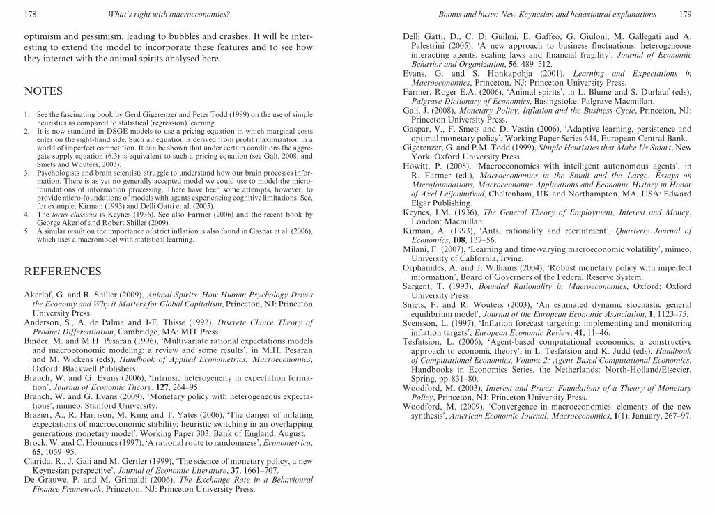
178 What’s right with macroeconomics?
optimism and pessimism, leading to bubbles and crashes. It will be inter-
esting to extend the model to incorporate these features and to see how
they interact with the animal spirits analysed here.
NOTES
1. See the fascinating book by Gerd Gigerenzer and Peter Todd (1999) on the use of simple
heuristics as compared to statistical (regression) learning.
2. It is now standard in DSGE models to use a pricing equation in which marginal costs
enter on the right- hand side. Such an equation is derived from profit maximization in a
world of imperfect competition. It can be shown that under certain conditions the aggre-
gate supply equation (6.3) is equivalent to such a pricing equation (see Galí, 2008; and
Smets and Wouters, 2003).
3. Psychologists and brain scientists struggle to understand how our brain processes infor-
mation. There is as yet no generally accepted model we could use to model the micro-
foundations of information processing. There have been some attempts, however, to
provide micro- foundations of models with agents experiencing cognitive limitations. See,
for example, Kirman (1993) and Delli Gatti et al. (2005).
4. The locus classicus is Keynes (1936). See also Farmer (2006) and the recent book by
George Akerlof and Robert Shiller (2009).
5. A similar result on the importance of strict inflation is also found in Gaspar et al. (2006),
which uses a macromodel with statistical learning.
REFERENCES
Akerlof, G. and R. Shiller (2009), Animal Spirits. How Human Psychology Drives the Economy and Why it Matters for Global Capitalism, Princeton, NJ: Princeton University Press.
Anderson, S., A. de Palma and J- F. Thisse (1992), Discrete Choice Theory of Product Differentiation, Cambridge, MA: MIT Press.
Binder, M. and M.H. Pesaran (1996), ‘Multivariate rational expectations models and macroeconomic modeling: a review and some results’, in M.H. Pesaran and M. Wickens (eds), Handbook of Applied Econometrics: Macroeconomics, Oxford: Blackwell Publishers.
Branch, W. and G. Evans (2006), ‘Intrinsic heterogeneity in expectation forma-tion’, Journal of Economic Theory, 127, 264–95.
Branch, W. and G. Evans (2009), ‘Monetary policy with heterogeneous expecta-tions’, mimeo, Stanford University.
Brazier, A., R. Harrison, M. King and T. Yates (2006), ‘The danger of inflating expectations of macroeconomic stability: heuristic switching in an overlapping generations monetary model’, Working Paper 303, Bank of England, August.
Brock, W. and C. Hommes (1997), ‘A rational route to randomness’, Econometrica, 65, 1059–95.
Clarida, R., J. Gali and M. Gertler (1999), ‘The science of monetary policy, a new Keynesian perspective’, Journal of Economic Literature, 37, 1661–707.
De Grauwe, P. and M. Grimaldi (2006), The Exchange Rate in a Behavioural Finance Framework, Princeton, NJ: Princeton University Press.
M3014 - SOLOW TEXT.indd 178 21/11/2012 13:03
Booms and busts: New Keynesian and behavioural explanations 179
Delli Gatti, D., C. Di Guilmi, E. Gaffeo, G. Giuloni, M. Gallegati and A. Palestrini (2005), ‘A new approach to business fluctuations: heterogeneous interacting agents, scaling laws and financial fragility’, Journal of Economic Behavior and Organization, 56, 489–512.
Evans, G. and S. Honkapohja (2001), Learning and Expectations in Macroeconomics, Princeton, NJ: Princeton University Press.
Farmer, Roger E.A. (2006), ‘Animal spirits’, in L. Blume and S. Durlauf (eds), Palgrave Dictionary of Economics, Basingstoke: Palgrave Macmillan.
Galí, J. (2008), Monetary Policy, Inflation and the Business Cycle, Princeton, NJ: Princeton University Press.
Gaspar, V., F. Smets and D. Vestin (2006), ‘Adaptive learning, persistence and optimal monetary policy’, Working Paper Series 644, European Central Bank.
Gigerenzer, G. and P.M. Todd (1999), Simple Heuristics that Make Us Smart, New York: Oxford University Press.
Howitt, P. (2008), ‘Macroeconomics with intelligent autonomous agents’, in R. Farmer (ed.), Macroeconomics in the Small and the Large: Essays on Microfoundations, Macroeconomic Applications and Economic History in Honor of Axel Leijonhufvud, Cheltenham, UK and Northampton, MA, USA: Edward Elgar Publishing.
Keynes, J.M. (1936), The General Theory of Employment, Interest and Money, London: Macmillan.
Kirman, A. (1993), ‘Ants, rationality and recruitment’, Quarterly Journal of Economics, 108, 137–56.
Milani, F. (2007), ‘Learning and time- varying macroeconomic volatility’, mimeo, University of California, Irvine.
Orphanides, A. and J. Williams (2004), ‘Robust monetary policy with imperfect information’, Board of Governors of the Federal Reserve System.
Sargent, T. (1993), Bounded Rationality in Macroeconomics, Oxford: Oxford University Press.
Smets, F. and R. Wouters (2003), ‘An estimated dynamic stochastic general equilibrium model’, Journal of the European Economic Association, 1, 1123–75.
Svensson, L. (1997), ‘Inflation forecast targeting: implementing and monitoring inflation targets’, European Economic Review, 41, 11–46.
Tesfatsion, L. (2006), ‘Agent- based computational economics: a constructive approach to economic theory’, in L. Tesfatsion and K. Judd (eds), Handbook of Computational Economics, Volume 2: Agent- Based Computational Economics, Handbooks in Economics Series, the Netherlands: North- Holland/Elsevier, Spring, pp. 831–80.
Woodford, M. (2003), Interest and Prices: Foundations of a Theory of Monetary Policy, Princeton, NJ: Princeton University Press.
Woodford, M. (2009), ‘Convergence in macroeconomics: elements of the new synthesis’, American Economic Journal: Macroeconomics, 1(1), January, 267–97.
M3014 - SOLOW TEXT.indd 179 21/11/2012 13:03

180 What’s right with macroeconomics?
APPENDIX: PARAMETER VALUES OF THE CALIBRATED MODEL
Heuristic Model
pstar 5 0; % central bank’s inflation target
a1 5 0.5; % coefficient of expected output in output equation
a2 5 −0.2; % a is interest elasticity of output demand
b1 5 0.5; % b1 is coefficient of expected inflation in inflation
equation
b2 5 0.05; % b2 is coefficient of output in inflation equation
c1 5 1.5; % c1 is coefficient of inflation in Taylor equation
c2 5 0.5; % c2 is coefficient of output in Taylor equation
c3 5 0.5; % interest smoothing parameter in Taylor equation
b 5 1; % fixed divergence in beliefs
d 5 2; % variable component in divergence of beliefs
gamma 5 1; % intensity of choice parameter
sigma1 5 0.5; % standard deviation shocks for output
sigma2 5 0.5; % standard deviation shocks for inflation
sigma3 5 0.5; % standard deviation shocks for Taylor equation
rho 5 0.5; % rho measures the speed of declining weights in mean
squares errors (memory parameter)
Rational Model
pstar 5 0; % central bank’s inflation target
a1 5 0.5; % coefficient of expected output in output equation
a2 5 −0.2; % a is interest elasticity of output demand
b1 5 0.5; % b1 is coefficient of expected inflation in inflation
equation
b2 5 0.05; % b2 is coefficient of output in inflation equation
c1 5 1.5; % c1 is coefficient of inflation in Taylor equation
c2 5 0.5; % c2 is coefficient of output in Taylor equation
c3 5 0.5; % interest smoothing parameter in Taylor equation
sigma1 5 0.5; % standard deviation shocks for output
sigma2 5 0.5; % standard deviation shocks for inflation
sigma3 5 0.5; % standard deviation shocks for Taylor equation
M3014 - SOLOW TEXT.indd 180 21/11/2012 13:03
181
7. The economics of the laboratory mouse: where do we go from here?
Xavier Ragot
Very few economists foresaw the economic and financial crisis that broke
out in 2007 and which has turned into the deepest world recession since
1929. Even worse, the field of economics may have prevented observers
from perceiving the first movements – the steady accumulation of eco-
nomic and financial fragility – of this extremely grave turbulence. It is
thus time to reassess the usefulness of current economic theory, but how
far should we go? How should a researcher in economics approach the
subject if he has come to perceive his work as being much like that of a
laboratory mouse? How can he advance his discipline, and therefore the
understanding of economics? And once the experimenters outside the cage
have placed the cheese, in which direction should he then search? What
needs to be changed in the research process of the discipline of economics?
The purpose of this chapter is primarily to identify what exactly needs to
be reconsidered in economics. The task consists in addressing the problem
for numerous rival research programmes: the exploration of the role of
rationality, financial imperfections and their nature, the importance of
comparison to the data, and so on. Beyond this diversity, we must seek
the principles of common methods to define the mainstream in econom-
ics. The question we then face is this: can the reform of economic thought
be achieved through modifying the dominant approach, or do we have to
search much farther afield?
Where will the new light come from to illuminate those obscure mech-
anisms that have brought economies to the brink of ruin? If we knew the
answer to that question, research would no longer be research, and we
would have already understood the crisis. So we have little alternative but
to compare the different research programmes, in other words, to observe
the mice and choose the best adapted. This, however, is still far from pro-
viding a solution to the problem, as we shall see. The selection criteria of
research programmes are themselves under debate: should they be able to
reproduce past historical data, make better predictions than the others, or
make fewer mistakes? And over what time horizon?
M3014 - SOLOW TEXT.indd 181 21/11/2012 13:03

182 What’s right with macroeconomics?
The first part of this chapter seeks to define the dominant current,
the mainstream. I define the mainstream, in brief, as the hypotheses of
equilibrium and absence of arbitrage opportunities, since recent works
show that the concept of rationality is becoming too narrow even for the
mainstream. Equilibrium does not necessarily mean stability. On the con-
trary, the multiplicity of equilibria is considered a sign of instability. On
the basis of this definition, one can attempt to identify recent works that
lie outside the mainstream. The second part of the chapter presents the
author’s research programme as an example of the endeavour to evolve
economic thought.
A REPRESENTATION OF THE DYNAMICS OF ECONOMIC RESEARCH PROGRAMMES: THE STANDARD PARADIGM
It is important to distinguish between the standard paradigm and the
world view of the profession. The latter attached central importance to
certain results – such as stability or efficiency. This was to the detriment of
other works showing the instability or inefficiency of market economies,
which were treated as theoretical curiosities. I start with a description of
the world view held by the majority of economists, before defining the
mainstream. I will then give some examples of very different research pro-
grammes that can be placed in the mainstream.
In early 2007, the most widely held economic view, as expressed in
journals, conferences and speeches, could be summed up as follows. The
market economy is stable and remarkably resistant to macroeconomic
shocks. The more developed the mechanisms of the market are, the
more resistant the economy is to shocks. In particular, the development
of capital markets has made it possible to divide up risk between dif-
ferent securities, so that each agent only bears a small share of the risk,
making the economy more stable. In more practical terms, the massive
securitization of US mortgages allowed banks to sell credit claims that
were evaluated by the discipline of the market. One of the vehicles of this
securitization was the infamous subprimes, the details of which I will not
go into here. More market means more stability. Moreover, allocation by
the market is generally efficient. Neo- Keynesian and neoclassical econo-
mists disagreed about the inefficiencies of economies: should the central
bank intervene to stabilize economies? Should fiscal policy be proactive?
Sometimes they should, sometimes not. The problem then lies in the quali-
fication of ‘sometimes’. Two different currents clearly emerged, associated
with identifiable policy options, but the models used in each case were very
M3014 - SOLOW TEXT.indd 182 21/11/2012 13:03
The economics of the laboratory mouse 183
similar and the methods were the same: the dynamic stochastic general
equilibrium model (DSGE).
Dynamic Stochastic General Equilibrium Models: a Genealogy
The DSGE models are largely inherited from the rational expectations
revolution of the early 1980s. The names associated with this change
of paradigm include Robert Lucas (1988), Thomas Sargent (Lucas and
Sargent, 1978), Finn Kydland and Edward Prescott (1977). This research
programme was based on a radical and forthright position. Starting with
the hypotheses that the economy functions perfectly and that the market
economy is efficient, what can one explain about economic fluctuations?
This approach was named real business cycle theory (RBC). It had spec-
tacular success as it greatly simplified the modelling strategy. With the
hypotheses of efficiency, the dynamics of the economy can be represented
by the choices of a representative agent who maximizes his or her utility;
he/she is capable of using all the resources of the economy but limited by
technological constraints. This research programme only gradually estab-
lished itself in economics, since many theorists found this view of the world
too simplistic, because it ignored the central question of aggregation. It
reduced macroeconomics to microeconomics, with one sole agent and one
good. The success of the RBC programme can be explained retrospectively
by the new relationship between theory and data. The economists working
on this research programme rigorously derived the implications for all the
economic variables of the models in order to test them econometrically.
Inside the RBC research agenda, a general movement has taken place in
the macroeconomic profession to confront the model rigorously with the
data using sophisticated econometric methods.
If nothing else, this shift of focus towards the data has shown the extent
to which the basic RBC model has been a spectacular scientific failure. The
basic model did not explain fluctuations in employment and asset prices
or the dynamics of inflation. In fact, it is difficult to give an example of
what the model explains in the data. All the anomalies were considered
as enigmas, stimulating research programmes that sought to improve the
match with the data by introducing additional frictions. Technological
frictions, strange preferences and diverse externalities were all introduced
into the model, but without ever really questioning the idea of a repre-
sentative agent and of econometric comparison with the data using the
appropriate filter.
One friction that enjoyed particular success was sticky prices. The
original RBC models (Cooley and Hansen, 1989) addressed the monetary
question on the basis of monetarist hypotheses. These models again met
M3014 - SOLOW TEXT.indd 183 21/11/2012 13:03

184 What’s right with macroeconomics?
with failure, leading to the introduction of monopolistic competition and
sticky nominal prices. This monetary dimension was all the more signifi-
cant since central banks had become important, if not the leading players
in macroeconomic stabilization. Developing theories likely to help central
banks in choosing their monetary policy became a very active field of
research.
The introduction of nominal rigidities into DSGE models was accom-
panied by another communication success – the rewording of the theoreti-
cal tool as a New Keynesian model: a representative agent allocates the
economy’s resources between consumption and saving on the one hand,
and work and leisure on the other, in the face of price rigidities. The term
‘Keynesian’ is always open to debate when applied to these models. The
basic New Keynesian models exclude involuntary unemployment and
possess perfect capital markets – two hypotheses that could hardly be
qualified as Keynesian. Can such models reproduce the observed dynam-
ics of the economy with reasonable parameters? The answer is far from
certain. A large number of additional hypotheses are introduced – what
are called ‘bells and whistles’ – to test these models, and the results are
sometimes good, sometimes very bad, especially in the financial part.
These models cannot explain the evolution of asset prices and exclude, by
hypothesis, any financial disequilibrium.
In 2007, the New Keynesian model had become the main tool of central
banks, international economic organizations, and even public administra-
tions. The approach to data, with devices such as Bayesian estimation, is
very sophisticated, which makes this tool very technical, although in itself
that is no guarantee of suitability. Nevertheless, this tool has become an
important part of the standard paradigm, used as an interface between
theoretical macroeconomics and empirical validation.
Faced with the ballooning number of additional hypotheses needed
to account for the data, economists have sought to define a central
method to impose some degree of intellectual discipline on the exercise.
Lucas highlighted two constraints: equilibrium and rationality. In DSGE
models, economies are always in equilibrium and agents always behave
rationally.
These DSGE models are now being condemned, but without really
being replaced by any new tools. The ‘initial’ New Keynesian models
adopted the hypothesis of perfect capital markets – a hypothesis at the
least exaggerated. The financial crisis did not call into question the models
themselves, but only this particular hypothesis about the functioning of
capital markets. Today, numerous works in central bank student research
programmes aim to ‘incorporate financial frictions into the DSGE model’.
Models of financial imperfection built in the 1990s, which had met with
M3014 - SOLOW TEXT.indd 184 21/11/2012 13:03
The economics of the laboratory mouse 185
some academic success within the standard paradigm while remain-
ing somewhat marginal, are now being used. The models of Nobuhiro
Kiyotaki and John H. Moore (1997), of Bengt Holmstrom and Jean Tirole
(1998), and others are now introduced into DGSE models. The hypotheses
of equilibrium and rationality are maintained, and financial frictions are
added in to match the model to the data.
This endeavour to improve DSGE models is the most active research
programme in macroeconomics, perhaps because of the importance of
central banks in the promotion of economic research. It is always difficult
to predict the success of this research programme or the nature of its possi-
ble successors. One a priori criticism that does appear legitimate, however,
is that this programme restricts itself to incremental modifications of exist-
ing models, and does not, therefore, allow for radical innovations, such
as the changing of models or more fundamental hypotheses. Very differ-
ent research programmes have developed within the standard paradigm,
gradually moving away from the hard core of hypotheses described above.
Each of these programmes existed before the crisis, which has altered their
scientific orientation and their relative importance within the academic
world.
Trade and Labour Market Frictions
The most important model, in terms of academic recognition, is prob-
ably that developed in the works of Peter Diamond (1982a, 1982b), Dale
Mortensen (Mortensen and Pissarides, 1994) and Christopher Pissarides
(2000). One of the origins of this model is the desire to understand market
exchange in more realistic representations of the market, notably with
decentralized transactions. At the heart of these models lies the assump-
tion that exchanges are bilateral operations conducted by agents who
meet at random on the market. The prices are fixed by the agents, once
they have met. For example, they may negotiate the price as a function of
their bargaining power. This model has been applied to markets for goods
and services and capital markets, but it is above all through its application
to the labour market that it has become an essential tool. It is fair to say
that it has even become the central model in that field, largely because it
can take into account involuntary (frictional) unemployment, which does
not exist in the so- called New Keynesian model. Criticisms have emerged
that call into question some of the standard hypotheses of this literature
(Shimer, 2005; Hall, 2005), but it appears that the central role of this
model in labour economics has not been affected by the crisis. It has grad-
ually been incorporated into macroeconomics (Merz, 1995; Andolfatto,
1996; Trigari, 2009), resulting in very complex models. Other attempts to
M3014 - SOLOW TEXT.indd 185 21/11/2012 13:03

186 What’s right with macroeconomics?
introduce involuntary unemployment into macroeconomics are currently
being developed.
Information
A set of very dynamic works are presently exploring the economic infor-
mation that agents use in making their choices. In their simple version,
rational expectations constitute a very strong hypothesis about the
information available to agents. Everyone has the same information and
uses that information optimally. At least four currents of research have
called this hypothesis into question. The first stems from the hypothesis
of information asymmetry, associated with the names of George Akerlof
(2007) and Joseph Stiglitz (2009), among others. These authors show that
if economic agents do not possess the same information, and in particu-
lar if one agent has more information than another, then the market is
prone to failure and government intervention can improve the function-
ing of the economy. The macroeconomic importance of information
asymmetries is difficult to assess. It appears to have had considerable
influence on the understanding of one market in particular: the credit
market. To simplify, the borrower generally has more information about
the quality of his or her projects than the lender does. He/she can use that
information asymmetry to negotiate a contract to his/her advantage, for
example to obtain financing for poor- quality projects that are purely for
his/her personal satisfaction. The lender, aware of this risk, will limit the
volume of credit. Consequently, credit rationing is a structural element
in the functioning of the credit market, justifying systematic public aid
for small businesses, for instance. But it is difficult to reconcile this view
of the credit market with the financial crisis, associated with an excess
of credit.
A second current of research on information does not address the
asymmetry of information between agents but the dispersion of infor-
mation across a large number of agents. Agents possess private informa-
tion and observe public information, which depends on the actions of
others – as in the case of share prices, for example. Each agent therefore
tries to figure out what the other agents expect, which in turn depends
on what the other agents think that each agent expects, and so on.
These ‘higher order expectations’ go back to John Maynard Keynes
and the beauty contest of chapter 12 of his work, General Theory of
Employment, Interest and Money, (1936 [1964]). These works have
assumed special theoretical importance with Stephen Morris and Hyun
Song Shin (Allen et al., 2006), and have been applied to the study of
economic fluctuations.
M3014 - SOLOW TEXT.indd 186 21/11/2012 13:03
The economics of the laboratory mouse 187
A third line of research concerns the cost of gathering and process-
ing information. If acquiring information is costly, agents may make a
rational choice not to acquire it, and therefore to accept a form of ‘rational
inattention’ (Sims, 2005).
A fourth approach to information focuses on the learning process.
Economic agents do not know the correct model of the economy (but the
economist who built the model does), and they gradually learn about the
environment in which they interact. The formation of economic expec-
tations is then dependent on the agents’ past history, for they can be
‘ mistaken’ over a long period of time.
These representations of the acquisition of information are important,
because they lay the foundations for many other frictions. On the labour
market, one can think of the constraints on unemployment benefits.
Should they be conditional, and if so, on what information? Our under-
standing of the functioning of capital markets is also highly dependent on
the way we represent informational problems.
Informational constraints have been incorporated into macroeconomics
essentially through the introduction of credit constraints. Some research
programmes seek to show how informational constraints can have a major
influence, through different channels, but as yet this research does not
appear to have been applied quantitatively.
A Definition of the Standard Paradigm
The previous section has described the diversity of research carried out
within the standard paradigm. From the variety of these works, we can
attempt to characterize the boundaries of the standard paradigm. Two key
concepts emerge.
The first is the idea of the absence of trade- off opportunities for charac-
terizing the behaviour of agents. This hypothesis is not as strong as that of
rational expectations, which defined the standard economics of the 1980s.
The hypothesis of rational expectations posits that agents make optimal
use of the information available to them. This hypothesis is relaxed in
works on rational inattention, which show that it can be ‘rational’ not to
use all the information when gathering or processing the information is
too costly. In such works, the volume of information processed is endog-
enous, and there are no trade- off opportunities: no individual could be
substantially better off by processing a different quantity of information
(otherwise they would do so).
Today, the hypothesis of rationality has therefore been weakened: it
now consists in imposing the following discipline. If the economist builds a
theory or a model in which the agents fail to do something that it is in their
M3014 - SOLOW TEXT.indd 187 21/11/2012 13:03

188 What’s right with macroeconomics?
interest to do, then the economist must justify why they did not do it; in
other words, the economist must explain agents’ rationality. In this sense,
the choices of economic agents are micro- founded.
A second hypothesis related to the absence of trade- off opportunities is
that agents can make economic predictions: in the language of economists,
this is the hypothesis of the formation of expectations. It is also subject
to the absence of trade- off opportunities, but more importantly, forming
expectations about the future requires some kind of equilibrium of the
economy. The definition of a concept of equilibrium is therefore essential.
This concept may vary from one article to another, but it remains central.
The first constraints on equilibria are of an accounting nature, and they
are always verified in the real world. If somebody sells something, then
somebody must buy something. This kind of relation is always true. Other
hypotheses on equilibria concern the interaction between individuals and
the degree of sophistication in their choices.
To sum up, standard economics can be defined by an absence of trade-
off opportunities and a concept of equilibrium. Not all macroeconomics
meets this definition. Research in the field of behavioural economics,
known as ‘agent- based modelling’, lies outside this framework. This
includes works by Giovanni Dosi (see Chapter 5 in this volume), Paul De
Grauwe (see Chapter 6 in this volume) and Willi Semmler (Chiarella et al.,
2009). They build models based on the assumption that economic agents,
households, firms or governments follow equations of behaviour that are
fixed a priori. The agents are then left to interact, statistically, to observe
how the economy evolves. So the aim is to simulate a virtual economy
with pre- defined behaviour. The behaviours that are chosen are derived
from the observation of real behaviour. The criticism levelled at standard
economics is that agents have every interest in adapting their behaviour in
response to changes in the environment, buying or selling less, employing
more, and so on. In other words, agents do not actually behave like eco-
nomic agents. The extent to which economic agents are rational remains
a central issue in economics. The battle of methods rages: the behavioural
approach and the standard economic approach throw a different light on
every subject. This can be considered a good thing, but in terms of policy
prescriptions, these approaches lead to different conclusions and are
therefore often incompatible.
The profession of economists is largely dominated by standard econom-
ics. The current crisis has nevertheless brought the battle of methods to the
fore. The issues of the stability of market economies and the existence of
financial bubbles have led economists to reconsider the rationality of indi-
vidual behaviour. The questions are not new, and neither, unfortunately,
are the answers.
M3014 - SOLOW TEXT.indd 188 21/11/2012 13:03
The economics of the laboratory mouse 189
Never Mind the Bottle . . .
The aim of this first section has not been to discuss critically the hypoth-
eses of the different research programmes; economics has suffered enough
from methodological quarrels. So instead of discussing only the hypoth-
eses, it is more instructive to discuss the results and compare them to the
data or experimental results. As Xavier Timbeau points out (see Chapter 1
in this volume), the latter affirmation is somewhat naive, since there is no
consensus in economics about what ‘comparison to the data’ really means.
But for the researcher, this is what makes economics so fascinating.
AN EXAMPLE RESEARCH PROGRAMME: THE RISK OF UNEMPLOYMENT
This second section presents the research programme of the author as
an example of the path followed by a laboratory mouse, to return to
the imagery of the introduction. Before describing the hypotheses of the
research programme, here is the substance. The aim is to present the eco-
nomic mechanisms or causalities before moving on to describe the method.
Representation of Risks in Macroeconomics
In macroeconomics, the risks faced by agents are often represented in
a simplistic manner. Most research works assume that households can
insure themselves against all possible risks and that the insurance market
functions perfectly. This hypothesis entails that households as a whole
only react to aggregate risks, such as movements of inflation, overall
growth, and so on.
To appreciate the extremely constraining nature of this hypothesis, one
need only look at the risk of unemployment. The hypothesis of a perfect
insurance market implies that households can (and want to) buy perfect
insurance against the risk of unemployment. This means that when their
status changes from employed to unemployed, their income should stay at
the same level, because their insurance should compensate for the loss of
wages. Consequently, the agents’ consumption should not decrease when
they become unemployed. This hypothesis of perfect insurance does not
correspond, however, to observations of the labour market. Admittedly,
state insurance mechanisms (the compensation rate varies between 40
and 90 per cent depending on the country and for a fixed period) and,
sometimes, private insurance, make up for the absence of earned income
in the case of a lay- off. Nevertheless, the compensation is far from perfect,
M3014 - SOLOW TEXT.indd 189 21/11/2012 13:03

190 What’s right with macroeconomics?
and household income falls in the event of unemployment. Empirical
estimations indicate a fall in consumption when agents lose their jobs (see
Carroll, 1992, for example).
Risks like that of unemployment concern individual agents, and they
can only be partly insured against. Economists call them ‘uninsurable idio-
syncratic risks’, because of the incomplete nature of insurance markets.
In addition to unemployment, health risks are also important in some
countries. In France, for example, the public health system provides
almost perfect insurance against the more serious health risks. In the
United States, where health care must be largely paid for by the patient’s
household, the risks of poor health are very serious, and one of the leading
causes of household bankruptcy (Chatterjee et al., 2007). Economists
sometimes consider uninsurable family risks, depending on the country. In
this case, ‘risk’ could mean having an unplanned child or divorcing, which
represents a net transfer to the lawyers.
Out of these different risks, unemployment is the most important for
two reasons. First, it is the most frequent risk causing a substantial loss of
income. Second, unemployment is endogenous to economic activity and a
natural subject of attention for the public authorities: by pursuing coun-
tercyclical policies or by modifying unemployment allowances, the public
authorities can easily alter the unemployment risk.
The risk of unemployment, like all uninsurable idiosyncratic risks, gives
rise to precautionary behaviour on the part of agents. When they expect
a rise in unemployment, they tend to consume less and to postpone the
purchase of durable goods in order to set aside some savings in case of
need. This fall in consumption can have a negative impact on production
because of the fall in aggregate demand. In turn, the fall in production
causes a rise in unemployment, creating a multiplier effect on the initial
rise in unemployment. This mechanism can be qualified as Keynesian
in the broadest sense: the rise in unemployment is caused by a fall in
aggregate demand (rather than effective, in this case) and an increase in
uncertainty.
Precautionary saving is therefore a mechanism related to a financial
imperfection, namely the absence of perfect insurance. This mechanism is
missing from most macroeconomic models, which assume the hypothesis
of perfect capital markets, allowing them to consider a representative
agent. There is a stream of research, however, that focuses on the role of
self- insurance, known as the macroeconomics of incomplete markets or
the macroeconomics of heterogeneous agents (because the hypothesis of
the representative agent no longer holds in these models). A third appel-
lation is the Bewley–Hugget–Aiyagari model, after three of the main
contributors. These works stand out first by their complexity: they call
M3014 - SOLOW TEXT.indd 190 21/11/2012 13:03
The economics of the laboratory mouse 191
for intensive computing, and the methods used to solve such models,
when all the individual behaviours have to be aggregated, continue to be a
subject of debate. Another reason for the low popularity of these models
is the relative uncertainty as to their importance for macroeconomics.
Per Krusell and Anthony A. Smith (1998) have shown that in some cases,
during average fluctuations in economic activity, the role of precaution-
ary saving appears to be negligible, and the hypothesis of a representative
agent is therefore valid.
Nevertheless, precautionary saving does seem to play an important role
during deep recessions when the risk of unemployment increases percepti-
bly (Challe and Ragot, 2011). On US data, we can identify a noticeable fall
in aggregate consumption due to precautionary saving. In addition, simple
tools can be developed to study precautionary saving in macroeconomics.
If the works mentioned above focus on precautionary saving in house-
holds, recent research investigates the behaviour of companies faced with
an increase in uninsurable uncertainty (Bloom, 2009; Arellano, 2008;
Arellano et al., 2011). In such cases, the rise in uncertainty leads firms to
reduce investment and postpone recruitment, thus contributing to the rise
in unemployment. The rise in precautionary saving also appears to have
affected financial intermediaries who have maintained large amounts of
liquidity with the central bank. Precautionary saving can therefore help
to explain the fall in private- sector credit. These mechanisms probably
played an important role in the financial crisis, and more precisely in its
impact on the real economy. Quantification of this impact and precise
discussion of the crisis lie outside the scope of this chapter, however.
Precautionary Saving in Incomplete Markets and Standard Economics
So the causalities proposed to explain the mechanism of precautionary
saving are based on agents’ expectations, on their rationality (they choose to
self- insure), and on the role of the equilibrium on the goods markets. If con-
sumption falls, so must the production of consumption goods, unless stocks
are to rise. The above research programme thus comes within the domain of
standard economics, encapsulated by the absence of trade- off opportunities
and by the concept of equilibrium. The author of these lines, endeavouring
to formalize Keynesian intuitions (in collaboration with Edouard Challe,
in many cases), thus finds himself at the heart of standard economics with
mathematical formalizations that are sometimes very unwieldy.
Non- standard formalizations of precautionary savings can be made.
For example, one can introduce, arbitrarily, a savings rate that increases
with the rate of unemployment. By exploring in more detail the rela-
tion between precautionary saving and the incompleteness of insurance
M3014 - SOLOW TEXT.indd 191 21/11/2012 13:03

192 What’s right with macroeconomics?
markets, we can better explain how unemployment benefits can limit
precautionary saving, or how the level of wage inequality influences the
aggregate effect of the rise in household risk. Precise analysis of the behav-
iour of microeconomic agents (assumed to be rational) extends the range
of possible experiments. The data appear to show that agents can make
mistakes in the evaluation of their idiosyncratic risk (of becoming unem-
ployed, for example). Consequently, the introduction of deviations from
rational expectations can be used to analyse the effects of over- optimistic
and over- pessimistic expectations.
CONCLUSION
The aim of this chapter is to shift the focus of the debate from the tools
to the theories and mechanisms. What are the fundamental mechanisms
lacking from economic understanding? From the answer to this pre-
liminary question, we can derive the tools and the (inevitably simplistic)
hypotheses required. The chapter started by seeking to define standard
economics before moving on to describe the author’s research programme.
It turns out that the latter lies within the bounds of standard economics,
which is neither good nor bad; it is simply not relevant.
The profession of economists is waiting for the understanding of new
mechanisms. There has been an effervescence in the work produced by
economists since the crisis, but the novelty of the work does not appear to
be on a par with the intellectual issues currently at stake. A new research
programme, or even a new paradigm, is needed. The question of what
tools it will use and how far they will rely on mathematics and computer
simulations remains entirely open. The only yardstick for the comparison
of research programmes is the relevance of the mechanisms brought to
light and their capacity to explain the data, although there will always be
disagreements about the nature of the relevant data. This affirmation is
above all normative, before being positive. In a nutshell, epistemology is
the revenge of the living cheese on the dead mouse.
REFERENCES
Akerlof, George (2007), ‘The missing motivation in macroeconomics’, American Economic Review, 97(1), 5–36.
Allen, F., S. Morris and H.S. Shin (2006), ‘Beauty contests and iterated expecta-tions in asset markets’, Review of Financial Studies, Oxford University Press for Society for Financial Studies, 19(3), 719–52.
M3014 - SOLOW TEXT.indd 192 21/11/2012 13:03
The economics of the laboratory mouse 193
Andolfatto, D. (1996), ‘Business cycles and labor market search’, American Economic Review, 86, 112–32.
Arellano, C. (2008), ‘Default risk and income fluctuations in emerging economies’, American Economic Review, 98(3), 690–712.
Arellano, C., Y. Bai and P. Kehoe (2011), ‘Financial markets and fluctuations in uncertainty’, Federal Reserve Bank of Minneapolis Working Paper.
Bloom, N. (2009), ‘The impact of uncertainty shocks’, Econometrica, 77(May), 623–86.
Carroll, C.D. (1992), ‘The buffer- stock theory of saving: some macroeconomic evidence’, Brookings Papers on Economic Activity, 1992(2), 61–156.
Challe, E. and X. Ragot (2011), ‘Fiscal policy in a tractable liquidity- constrained economy’, Economic Journal, 121(551), 273–317.
Chatterjee, S., D. Corbae, M. Nakajima and J.- V. Ríos- Rull (2007), ‘A quantita-tive theory of unsecured consumer credit with risk of default’, Econometrica, 75(6), 1525–89.
Chiarella, C., P. Flaschel, H. Hung and W. Semmler (2009), Business Fluctuations and Long- phased Cycles in High Order Macrosystems, New York: Nova Publishers.
Cooley, T.F. and G.D. Hansen (1989), ‘The inflation tax in a real business cycle model’, American Economic Review, 79(4), 733–48.
Diamond, P. (1982a), ‘Demand management in search equilibrium’, Journal of Political Economy, 90, 881–94.
Diamond, P. (1982b), ‘Wage determination and efficiency in search equilibrium’, Review of Economic Studies, 49, 217–27.
Hall, R.E. (2005), ‘Employment fluctuations with equilibrium wage stickiness’, American Economic Review, 95(1), 50–65.
Holmstrom, B. and J. Tirole (1998), ‘Private and public supply of liquidity’, Journal of Political Economy, 106(1), 1–40.
Keynes, J.M. (1936 [1964]), General Theory of Employment, Interest and Money, Orlando, FL: First Harvest/Harcourt Inc.
Kiyotaki, N. and J. Moore (1997), ‘Credit cycles’, Journal of Political Economy, 105(2), 211–48.
Krusell, P. and A.A. Smith Jr (1998), ‘Income and wealth heterogeneity in the macroeconomy’, Journal of Political Economy, 106(5), 867–96.
Kydland, F.E. and E.C. Prescott (1977), ‘Rules rather than discretion: the incon-sistency of optimal plans’, Journal of Political Economy, 85(3), 473–91.
Lucas, R.E. (1988), ‘What economists do’, Journal of Applied Economics, May, pp. 1–4.
Lucas, R. and T. Sargent (1978), ‘After Keynesian macroeconomics’, in Federal Reserve Bank of Boston, After the Phillips Curve: Persistence of High Inflation and High Unemployment, proceedings of conference held in June 1978, The Federal Reserve Bank of Boston Conference Series, no. 19, pp. 49–72.
Merz, M. (1995), ‘Search in the labor market and the real business cycle’, Journal of Monetary Economics, 36(2), 269–300.
Mortensen, D. and C. Pissarides (1994), ‘Job creation and job destruction in the theory of unemployment’, Review of Economic Studies, 61, 397–415.
Pissarides, C. (2000), Equilibrium Unemployment Theory, 2nd edn, Cambridge, MA: The MIT Press.
Shimer, R. (2005), ‘The cyclical behavior of equilibrium unemployment and vacancies’, American Economic Review, 95(1), 25–49.
M3014 - SOLOW TEXT.indd 193 21/11/2012 13:03

194 What’s right with macroeconomics?
Sims, C. (2005), ‘Rational inattention: a research agenda’, Deutsche Bundesbank, Research Centre, Discussion Paper Series 1: Economic Studies no. 2005, 34.
Stiglitz, Joseph E. (2009), ‘The current economic crisis and lessons for economic theory’, Eastern Economic Journal, 35(3), 281–96.
Trigari, A. (2009), ‘Equilibrium unemployment, job flows, and inflation dynamics,’ Journal of Money, Credit and Banking, 41(1), 1–33.
M3014 - SOLOW TEXT.indd 194 21/11/2012 13:03
195
8. Round table discussion: where is macro going?
Wendy Carlin, Robert J. Gordon and
Robert M. Solow
Robert M. Solow (MIT) A round table about the current state or the
future of macroeconomics should not start from the opposition of good
and bad models. Even the simplest fundamentalist dynamic stochastic
general equilibrium (DSGE) models contain a certain amount of ordi-
nary common- sense economics that no one would be against in principle.
In response to criticism, the naive versions of that kind of model have
been fixed up with some financial intermediation, with sticky prices, with
what are now called ‘rule- of- thumb’ consumers. It is better not to try to
take positions for or against the whole school of modelling, which has
good things and bad things about it, but to try to be careful about what
characteristics of that modelling style one likes or doesn’t like.
What particularly sets my teeth on edge is the prominent role that gets
played by forward- looking, relatively unconstrained consumer- worker-
owners. I don’t know whether the New Keynesian Phillips curve is new,
but it’s certainly neither Keynesian nor a Phillips curve, but I guess that’s
pretty good, as far as nomenclature goes. I suspect that nearly all consum-
ers are rule- of- thumb consumers and rule- of- thumb labour suppliers, not
necessarily because they’re liquidity constrained, but for various reasons:
because they’re boundedly rational, or they don’t care, or they do what
their parents did, and so on. I thought it was interesting to see what Paul
De Grauwe [Chapter 6] can do with such a simple version of rule- of-
thumb consumers. I think the key reason why I baulk at the forward-
looking, relatively unconstrained consumer- worker- owner is because that
device imposes more intertemporal coherence on economic time series
than we have any reason to suspect economic time series to have. Even if
individual consumers obey Euler equations (although there is no empirical
evidence of anyone ever obeying a Euler equation), there is absolutely no
reason to believe that aggregate consumption would obey such an equa-
tion. So that’s my particular irritation, and remember what I said at the
M3014 - SOLOW TEXT.indd 195 21/11/2012 13:03

196 What’s right with macroeconomics?
beginning: a lot in those models is perfectly acceptable and is just ordinary
economics.
We have two contributors in the discussion: Wendy Carlin of University
College London and Bob Gordon of Northwestern University. After their
presentations, we will open up the debate.
Wendy Carlin (University College London) The subject of my presen-
tation is ‘Macroeconomic paradigms, policy regimes and the crisis: the
origins, strengths and limitations of Taylor Rule macroeconomics’. Bob
[Solow] provided a nice introduction to the themes I want to develop.
I’d like to start with the point that Bob has made about how we should
characterize the mainstream macro model and the policy regime before
the crisis, and I’ll refer to both narrow and broad versions of what I’m
going to call ‘Taylor Rule macro’. In the second part I will look at where
Taylor Rule macroeconomics came from, since it’s the focus around which
many of the contributions to this volume have centred. To do that, I want
to draw a connection between the rather rare events of global economic
crisis, macro models, or paradigms, and policy regimes. The third part
will focus specifically on the Taylor principle and stabilization so as to
highlight some good and bad things in Taylor Rule macro. I will use three
examples: the eurozone, the causes of the global crisis, and the issue of
post- crisis management. I’ll finish with a point or two about where we go
from here.
Figure 8.1 is the narrow version of mainstream macro that Bob was
referring to. It’s a very linear structure. We start with the neoclassical
growth model, and then add rational expectations and technology shocks
Neoclassical growth model
Real business cycle model
New Keynesian DSGEmodel: IS/PC/MR
+ rational expectations,technology shocks
+ money, imperfectcompetition in goodsmarket, sticky prices
Figure 8.1 Mainstream macroeconomics pre- crisis: narrow version
M3014 - SOLOW TEXT.indd 196 21/11/2012 13:03
Round table discussion 197
with a particular kind of structure, which Paul De Grauwe brought out
very clearly in his contribution [Chapter 6]. This produces the real business
cycle (RBC) model. Next, we add money, imperfect competition in goods
markets and sticky prices, and we get the canonical New Keynesian DSGE
model, with the three famous equations: the Euler equation form of the
(IS), the Phillips curve (PC) – recognizable or not, as Bob says – and the
monetary rule (MR). So that’s the narrow version.
The broad version of mainstream macro is depicted in Figure 8.2. It can
be thought of as comprising three blocks: a demand block, with liquidity-
constrained and unconstrained households and firms; a supply block with
imperfectly competitive goods and labour markets; and a policy block
with a forward- looking central bank. Once again, we’ve got the three-
equation structure: the IS, the PC and the MR. The associated macroeco-
nomic policy regime has come to be known as Taylor Rule macro because
of the central role on the policy side played by the Taylor Rule.
We can see in Figure 8.3 that narrow and broad versions of Taylor
Rule macro come from different ‘lineages’. Paul De Grauwe [Chapter 6]
develops the broad version using very different behavioural assumptions,
but with the same blocks. This is a way of thinking about a wide variety
of models in the mainstream and close to the mainstream, of the sort
that Volker Wieland [Chapter 2] has included in his large set for model
comparison. So what’s wrong with this? Obviously the big problem is that
irrespective of whether you have the broad or the narrow version, these
Liquidity-constrained &unconstrained households & firms
(IS)
Imperfectly competitive goods &labour markets (PC)
Forward-looking central bank (MR)
Taylor Rule macro IS/PC/MR
Figure 8.2 Mainstream macroeconomics pre- crisis: broad version
M3014 - SOLOW TEXT.indd 197 21/11/2012 13:03

198 What’s right with macroeconomics?
mainstream models were unable to provide a good explanation for the
crisis that we faced – never mind being able to predict it! Both versions
omitted the financial sector. So let me use that to lead into the question
of where a rules- based policy regime centred on the Taylor principle came
from.
Global crises are very rare events. After each of the two global crises of
the Great Depression and the Great Stagflation, a new macroeconomic
paradigm emerged, associated with a new policy regime and followed by
a couple of decades of satisfactory performance (see Figure 8.4). Then,
what I call ‘inattention’ developed, and another global crisis occurred. We
are familiar with that pattern in relation to the Great Depression: Keynes
developed his General Theory of Employment to account for persistent
involuntary unemployment, within which the voluntary- only unemploy-
ment equilibrium could be nested as a special case. A new macro policy
regime, both at the national and international levels, developed and the
decades of the Golden Age followed. This model and policy regime,
however, didn’t pay proper attention to what was going on below the
surface of good macro performance during the Golden Age, and it was
inattentive to supply shocks and to the role of expectations. So, once
the inflationary shocks emerged, the existing policy regime gave the
Mainstream Taylor Rule macro before the crisis
Liquidity-constrained &unconstrained households &
firms (IS)
Imperfectly competitivegoods & labour markets (PC)
Forward-looking central bank(MR)
Neoclassical growth model
Real business cycle model
New Keynesian DSGE model:IS/PC/MR
Taylor Rule macro IS/PC/MRPolicy regime:
Missing: thefinancial sector
‘Broad’‘Narrow’
Figure 8.3 Mainstream macroeconomics pre- crisis: narrow vs. broad
M3014 - SOLOW TEXT.indd 198 21/11/2012 13:03
Round table discussion 199
wrong signals, and we ended up with the next crisis, which was the Great
Stagflation of the 1970s and early 1980s.
Going through the same steps, we can see that in the aftermath of the
Great Stagflation there was a shift in thinking. A new paradigm emerged
centred on rational expectations and the Lucas critique, and out of that
came the new policy regime – Taylor Rule macro. This was followed by
good performance and the Great Moderation. Yet once again, something
was building up beneath the surface of tranquillity. We can think of it in
terms of what was happening in the financial sector and in the build- up of
imbalances of various kinds – both private- sector imbalances and imbal-
ances between countries. Then the global financial crisis came. If we put
these two cycles together, we can ask whether the improved macroeco-
nomic performance on the back of each new policy regime didn’t contain
the seeds of a new source of instability that had the potential to incubate
the next global crisis.
This brings to the fore the question of whether a process is underway of
moving to a new macroeconomic paradigm and policy regime, and if so,
whether it will contain the seeds of the next crisis. A lot of the contribu-
tions to this volume focus on macroeconomic modelling at business cycle
GreatDepression
Keynes’economics
Inattention:supply shocks& expectations
Demandmanagement
& Bretton WoodsGolden Age
REH/Lucascritique
GreatStagflation
Taylor RuleMacro
GreatModeration
Inattention:finance &
imbalances
GlobalFinancial
Crisis
Figure 8.4 From the Great Depression to the global financial crisis
M3014 - SOLOW TEXT.indd 199 21/11/2012 13:03

200 What’s right with macroeconomics?
frequency. Is there a link between a business cycle orientation, which
characterized both the Keynesian paradigm and the Taylor Rule para-
digm, and the cycle of global crisis–new paradigm–new policy regime–
satisfactory performance–next crisis?
Figure 8.5 shows a U- shaped pattern from just before the Great
Depression to just before the global financial crisis in the share of income
received by the top 1 per cent of taxpayers in the USA (Saez and Piketty,
2003). In 1928, 24 per cent of income was in the hands of 1 per cent of
taxpayers in the USA; the share fell to a trough in 1975–76, and then rose
until it was back to 24 per cent in 2007. Shifts in distribution happen at
much lower frequency than the business cycle and may be important for
understanding crises.
Figure 8.6 is taken from the work of Thomas Philippon and Ariell
Reshef (2009) and reveals another big U- shaped pattern of this kind for
the USA. The solid line captures an index of financial regulation: there
was an increase in regulation from the 1930s – the bottom of the U- shape
occurred during the Golden Age – and then financial deregulation began
from the early 1980s. The line with markers is the ratio of wages in the
financial sector to average wages in the economy. We can see that the
financial sector became very boring during the Golden Age: there was no
USA: percentage of income received by the top 1 per cent of taxpayers(including capital gains), 1913–2008
0%
5%
10%
15%
20%
25%
30%
1913
1918
1923
1928
1933
1938
1943
1948
1953
1958
1963
1968
1973
1978
1983
1988
1993
1998
2003
2008
2007: 24%1928: 24%
Source: The World Top Incomes Database available at
http://g- mond.parisschoolofeconomics.eu/topincomes/ (accessed 22 August 2011).
Figure 8.5 USA: percentage of income received by the top 1 per cent of
taxpayers
M3014 - SOLOW TEXT.indd 200 21/11/2012 13:03
Round table discussion 201
wage premium for working there. But with financial deregulation, that
premium re- emerged, and by the mid- 2000s had returned to the level of
the 1920s.
For the Golden Age and after, Figure 8.7 shows the evolution of the
share of labour in GDP (workers’ compensation corrected for changes
in self- employment) for the USA and for 15 other OECD countries.
The wage share rose through the Golden Age, peaked during the Great
Stagflation, and then declined in the run- up to the global financial crisis.
In the lower panel of Figure 8.7, the stagnant level of real wages in the
bottom part of the labour market in the USA is shown. Measured in 2009
US dollars, the minimum wage peaked in 1968. The average real wage of
production workers increased to $22 per hour in 1978 and was about the
same level in real terms in the 2000s.
Is there a connection between these low- frequency changes in distribu-
tion and the kinds of crisis that we have experienced? In the run- up to the
Great Stagflation, there was a shift in bargaining power towards workers –
this was an important component of the supply- side shocks that produced
high inflation and the sharp recessions of the early 1980s. We have seen the
reverse happening in the period since the early 1980s.
The idea that shifts in distribution could be linked to financial fragility
–3
–2.5
–2
–1.5
–1
–0.5
0
0.5
1
1
1910
1920
1930
1940
1950
1960
1970
1980
1990
2000
1.1
1.2
1.3
1.4
1.5
1.6
1.7
Relative wage in finance Financial deregulation index
Source: Philippon and Reshef (2009).
Figure 8.6 Relative wages in the financial sector and financial
deregulation, USA
M3014 - SOLOW TEXT.indd 201 21/11/2012 13:03

202 What’s right with macroeconomics?
in the run- up to the global financial crisis was discussed by Raghuram
Rajan (2010) and formalized in a recent paper by Michael Kumhof and
Romain Rancière (2010). A shift in bargaining power and in between-
group inequality is crucial to generating financial fragility in their model;
we should think about how to include this mechanism in our macroeco-
nomic framework. The shock is a shift in wage inequality, as illustrated in
the stylized facts in the earlier figures. More detailed data show that in the
USA, consumption inequality rose less than income inequality and that
debt- to- income ratios outside the top 5 per cent of households increased.
This suggests that there was a nascent weakness of aggregate demand
caused by the distributional shift, for which the solution required workers’
indebtedness to rise.
In this way, we can see a possible connection between the big shifts in
income distribution, the growth of credit and the link to financial fragility.
By connecting the wage squeeze, as I’ve called it, to financialization, credit
growth and the leverage cycle, we have an explanation for the so- called
05
10152025
1964
1960
1968
1976
1972
1980
1988
1984
1992
1996
2000
2004
1964
1960
1968
1976
1972
1980
1988
1984
1992
1996
2000
2004
USA Real average hourlycompensation, production &non-supervisory workers, 2009$
USA Real hourly minimum wage 2009$
50
55
60
65
70
75
80
Share of wages in GDP, %, USAShare of wages in GDP,OECD (15 countries excl. USA)
Sources: Data on real average compensation and real hourly minimum wages are from
Economic Policy Institute (EPI) http://www.stateofworkingamerica.org/files/files/Wages_
minwage.xlsx adjusted to 2009$ and http://www.stateofworkingamerica.org/files/files/3B_
hourly_wage_and_comp_growth.xlsx; Wage shares from Glyn (2009).
Figure 8.7 The wage squeeze in the USA and OECD, 1960–2007
M3014 - SOLOW TEXT.indd 202 21/11/2012 13:03
Round table discussion 203
‘Greenspan Put’: low interest rates were required in order to stabilize
domestic demand. This relates to Taylor’s argument that the US Board
of Governors of the Federal Reserve System (the Fed) failed to increase
interest rates in the early 2000s in line with his rule. If, however, an under-
lying weakness of aggregate demand (associated with the distributional
effects) had lowered the neutral interest rate, then the Fed may have been
justified in keeping rates low to encourage households to borrow and
spend within a Taylor- rule macro framework.
As the Taylor Rule has played a part in most of the contributions to
this volume, I will take three examples to suggest its role in macroeco-
nomic models and policy in the future. I want to talk very briefly about
the eurozone crisis. I will argue that Taylor Rule macro had something to
contribute, but was largely ignored. Ireland and Spain had negative real
interest rates for most of the eurozone’s first decade. There was no Taylor
principle equivalent in place in the member countries’ national policy
regimes to promote stabilization.
Take the example of a very simple, country- specific inflation shock
occurring in one eurozone country. Before turning to the case of a euro-
zone member, think first of all of what would happen under flexible
exchange rates: with a positive inflation shock, the central bank and the
foreign exchange market forecast the output contraction that’s required
to get back to target inflation. So the central bank raises the interest rate,
the exchange rate appreciates, a negative output gap emerges and the
economy is guided back to equilibrium with target inflation; all real varia-
bles are unchanged. This is just the optimal Taylor Rule. Now think of the
same temporary, country- specific inflation shock in a eurozone member.
Let’s assume that a fiscal policy rule was used to implement exactly the
same Taylor Rule optimal output and inflation path back to target – that
is, the eurozone inflation target – as under flexible exchange rates. Once
we’re back at equilibrium, however, the home country’s real exchange rate
has appreciated due to higher inflation along the path back to equilibrium.
Consumption and investment are unchanged, the real interest rate is back
at the eurozone real interest rate, but net exports are lower, so the fiscal
balance must have deteriorated. This very simple example shows that
fiscal imbalance in this case arises not because of any ‘profligacy’, but
due to implementing the same optimal policy rule as chosen by a flexible
exchange rate central bank. But even that version of the Taylor Rule was
not used by member countries in the eurozone.
The rule for stabilization for a member country requires something
more than just getting back to eurozone target inflation. Policy makers
have to deliver output at equilibrium, inflation at the eurozone target and
a real exchange rate consistent with primary fiscal balance. That’s a much
M3014 - SOLOW TEXT.indd 203 21/11/2012 13:03
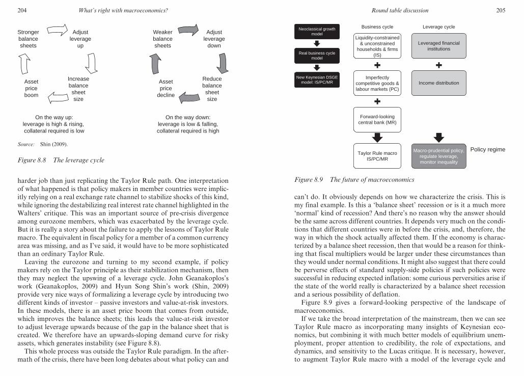
204 What’s right with macroeconomics?
harder job than just replicating the Taylor Rule path. One interpretation
of what happened is that policy makers in member countries were implic-
itly relying on a real exchange rate channel to stabilize shocks of this kind,
while ignoring the destabilizing real interest rate channel highlighted in the
Walters’ critique. This was an important source of pre- crisis divergence
among eurozone members, which was exacerbated by the leverage cycle.
But it is really a story about the failure to apply the lessons of Taylor Rule
macro. The equivalent in fiscal policy for a member of a common currency
area was missing, and as I’ve said, it would have to be more sophisticated
than an ordinary Taylor Rule.
Leaving the eurozone and turning to my second example, if policy
makers rely on the Taylor principle as their stabilization mechanism, then
they may neglect the upswing of a leverage cycle. John Geanakoplos’s
work (Geanakoplos, 2009) and Hyun Song Shin’s work (Shin, 2009)
provide very nice ways of formalizing a leverage cycle by introducing two
different kinds of investor – passive investors and value- at- risk investors.
In these models, there is an asset price boom that comes from outside,
which improves the balance sheets; this leads the value- at- risk investor
to adjust leverage upwards because of the gap in the balance sheet that is
created. We therefore have an upwards- sloping demand curve for risky
assets, which generates instability (see Figure 8.8).
This whole process was outside the Taylor Rule paradigm. In the after-
math of the crisis, there have been long debates about what policy can and
Adjustleverage
up
Increasebalancesheetsize
Assetpriceboom
Strongerbalancesheets
Adjustleverage
down
Reducebalancesheetsize
Assetprice
decline
Weakerbalancesheets
On the way up:leverage is high & rising, collateral required is low
On the way down:leverage is low & falling,collateral required is high
Source: Shin (2009).
Figure 8.8 The leverage cycle
M3014 - SOLOW TEXT.indd 204 21/11/2012 13:03
Round table discussion 205
can’t do. It obviously depends on how we characterize the crisis. This is
my final example. Is this a ‘balance sheet’ recession or is it a much more
‘normal’ kind of recession? And there’s no reason why the answer should
be the same across different countries. It depends very much on the condi-
tions that different countries were in before the crisis, and, therefore, the
way in which the shock actually affected them. If the economy is charac-
terized by a balance sheet recession, then that would be a reason for think-
ing that fiscal multipliers would be larger under these circumstances than
they would under normal conditions. It might also suggest that there could
be perverse effects of standard supply- side policies if such policies were
successful in reducing expected inflation: some curious perversities arise if
the state of the world really is characterized by a balance sheet recession
and a serious possibility of deflation.
Figure 8.9 gives a forward- looking perspective of the landscape of
macroeconomics.
If we take the broad interpretation of the mainstream, then we can see
Taylor Rule macro as incorporating many insights of Keynesian eco-
nomics, but combining it with much better models of equilibrium unem-
ployment, proper attention to credibility, the role of expectations, and
dynamics, and sensitivity to the Lucas critique. It is necessary, however,
to augment Taylor Rule macro with a model of the leverage cycle and
Neoclassical growthmodel
Real business cyclemodel
New Keynesian DSGEmodel: IS/PC/MR
Business cycle
Liquidity-constrained& unconstrained
households & firms(IS)
Imperfectlycompetitive goods &labour markets (PC)
Forward-lookingcentral bank (MR)
Taylor Rule macroIS/PC/MR
Leverage cycle
Leveraged financialinstitutions
Income distribution
Macro-prudential policy,regulate leverage,monitor inequality
Policy regime
Figure 8.9 The future of macroeconomics
M3014 - SOLOW TEXT.indd 205 21/11/2012 13:03

206 What’s right with macroeconomics?
connect this way of thinking about macro with income distribution. In
Figure 8.9, the DSGE model has shrunk a bit up into the left- hand corner.
This is not to say that this work and methodology are not extremely pow-
erful and important, but that it should be at the service of building and
improving the macroeconomic framework and policy regime. It shouldn’t
dictate or define those things; it should simply be seen as a powerful mod-
elling tool. We need to build good models of the leverage cycle, and to
incorporate distributional effects of the kinds I have suggested.
Robert J. Gordon (Northwestern University) Throughout my presenta-
tion, I will take an American perspective for two reasons: first, because
American authors have dominated the development of business cycle
theory over the last 50 years, and, second, because we all agree that the
worldwide crisis started in 2007 with the American subprime mortgage
market and the debacle of US financial markets. Exclusively, I’m going
to be talking about closed- economy, business- cycle macro, excluding
international macro and long- run growth issues.
For me, the basic unanswered questions are: why are some slumps
long and intractable while other downturns are quickly reversed? Do the
answers clarify the co- existence in our history of the Great Depression,
the Japanese Lost Decade (now becoming two decades), and the Great
Moderation followed by the Great American Slump?
I’m going to focus on what we can learn from history about shocks and
propagation mechanisms, and then move on to modern macro, which is
largely the DSGE models. I will then try to convince you that not only do
the DSGE models have the wrong set of shocks, or at least an incomplete
list of shocks, but they also miss many of the propagation mechanisms
that are essential to explaining the history with which I begin.
The emphasis on shocks is highlighted by the debate among US econo-
mists. Up until three years ago, all that anybody talked about was, ‘What
was the source of the Great Moderation? Was it diminished shocks or
better behaviour by the Fed?’ This debate was summarily ended by the
post- 2007 crisis, because ‘poof!’, the Great Moderation went away. But
the emergence of the crisis highlighted the fact that Alan Greenspan –
unlike the name that had been given to him by the famous journalist Bob
Woodward in his book on Greenspan called ‘Maestro’ (Woodward, 2000)
– far from being a maestro, was just plain lucky. He was particularly lucky
that his term ran out in January 2006 at the height of the bubble, leaving
poor hapless Ben Bernanke to come in and clean up what Greenspan had
left behind. There wasn’t any great performance by the Fed in the 20 years
before 2007. It was the same old Fed; it just benefited from 20 years of
reduced shocks. The Fed fuelled the housing bubble by deviating from
M3014 - SOLOW TEXT.indd 206 21/11/2012 13:03
Round table discussion 207
Taylor’s Rule (and I agree with John Taylor’s very insistent, repeated
claims to that effect), but also by defaulting on its own duty to regulate
financial institutions, again partly because of Greenspan’s doctrinaire
opposition to regulation.
Figure 8.10 displays the output gap for the United States since 1950.
It looks almost identical to the graph in Paul De Grauwe’s contribution
[Chapter 6]. The only difference is that in his graph, the recent output gap
only went down to about −6 per cent, and here it goes down to −8 per cent.
That’s not because of a different measurement technique; it’s because the
GDP data were revised in July 2010 to show a substantially steeper decline
in US GDP over 2008–10 than in the earlier data. This graph shows that
the economy can be both overheated and ice- cold, with all the gradations
in between. Let me point out some of the things you see here: we had an
overheated economy during the Vietnam War, which is well- known –
that’s when the great acceleration of inflation occurred – and a similarly
overheated economy in the Korean War era. The recent great crisis and
recession in the USA looks about the same in its maximum negative
output gap as in 1982. The big difference, however, is when you look at
how fast that gap was eliminated in 1983–84 as compared to 2009–10.
A traditional taxonomy of shocks distinguishes three different types:
private- sector demand shocks, government- created demand shocks, and
then the supply shocks, which have been almost entirely neglected in the
literature of the last 20 years by the so- called New Keynesian Phillips
curve. It’s helpful to divide up, initially, the private- sector demand shocks
into the four categories of expenditure on GDP, consumption, investment,
1950 1955 1960 1965 1970 1975 1980 1985 1990 1995 2000 2005 2010–10
–8
–6
–4
–2
0
2
4
6
8GDP Gap (Actual minus potential real GDP, log percentage ratio)
Figure 8.10 GDP gap
M3014 - SOLOW TEXT.indd 207 21/11/2012 13:03

208 What’s right with macroeconomics?
government spending and net exports. This first list of shocks is adequate
to understand most of the post- war period, but it is certainly not enough
to understand either 1929–33 or post- 2007. Direct shocks to consumption
are minor. Consumption behaviour is better categorized as a propaga-
tion mechanism, particularly the role of consumption in responding to
wealth bubbles or changes in real wealth, including the effect of changes
in household liabilities in the aftermath of wealth bubbles. This goes
back to Franco Modigliani’s life-cycle hypothesis, which formally intro-
duced wealth effects into Keynesian macro. The heart of instability in
the private sector is unstable investment, particularly for residential and
non- residential structures. It’s part of the Keynesian heritage, based on
the central concepts of coordination failures and long slumps following
overbuilding.
One may ask if the problem is overbuilding or over- indebtedness. The
two things go together: in a cycle of overbuilding such as in the late 1920s,
structures are financed by debt, and the economy is left with see- through
vacant office buildings and a hangover of debt. The residential construc-
tion instability was aggravated by the peculiar US financial market regu-
lations before 1980 that made residential construction a sort of residual
afterthought of financial markets. Residential construction would collapse
through quantitative rationing whenever tight money was introduced.
Government military spending created a lot of instability between 1940
and 1973, but then it became too small to matter, and even the Iraq and
Afghanistan wars have not caused enough variation in government spend-
ing share of GDP even to notice. At times net exports matter, mainly as a
propagation mechanism, particularly in 1980 to 1985, when tight money
and fiscal easing caused a dollar appreciation and a collapse in net exports.
Residential and non- residential structures are at the centre of old-
fashioned, traditional Keynesian macro. Structures are inherently subject
to overbuilding because of long gestation lags. Different people get the
uncoordinated idea that it would be great to build an office building at
the corner of Wacker and Madison in Chicago. Except four people get the
same idea, and they each manage to convince banks to finance them, when
only one building is needed. And all four eventually get built and wind up
vacant. The developers may fail, and the buildings may be sold for half
of their construction costs, and the economy is left with this hangover of
vacant buildings and over- indebtedness. This happened not just in the
1920s, but in the last few years. The Wall Street Journal reported in 2010:
‘In Las Vegas numerous multi- billion- dollar casino- hotel projects have
halted construction midway’; ‘Hotel rooms are wildly overbuilt’; and
‘There won’t be another casino property built in Las Vegas for a decade’.
There was no tall building of any kind built in Chicago or New York
M3014 - SOLOW TEXT.indd 208 21/11/2012 13:03
Round table discussion 209
during the entire decade of the 1930s, and the tallest building in Chicago
was the Board of Trade from 1930 until 1957. The tallest building in New
York was the Empire State Building from 1931 until 1973 when the World
Trade Centre was built.
Let’s move on to the second main source of shocks, government- created
demand shocks. We had volatile military spending in World War Two,
and in the Korean and Vietnam wars. This ties in with the Barro paradox,
as I call it, about estimating fiscal multipliers: we only get variation in gov-
ernment spending in wartime when we have capacity constraints, and we
don’t get much variation that we can see in periods when the economy has
a lot of excess capacity, as it does now. We should also add to the list of
sources of government- caused instability demand shocks caused by tight
money when the Fed decides to fight inflation. That also means that we
need an inflation model to explain the sources of inflation that become in
turn the motivation for tight money. The history of the Phillips curve is
well known, and I have a recent survey paper on it (Gordon, 2011). There
was the dilemma, so well described by Paul Samuelson and Robert Solow
in 1959: how come inflation started taking off in the mid- 1950s in the USA
before it appeared that full capacity had been reached? The initial Phillips
curve, as it was christened by Samuelson and Solow in the American
Economic Association (AEA) meetings in 1959, involved a negative trade-
off, and they were rightly sceptical, even then, that this would be perma-
nent or could be exploited. But the formal destruction of the permanent,
negatively- sloped Phillips curve, which was actually taken seriously –
particularly by the Democratic administration in the 1960s – was achieved
by the natural rate hypothesis of Milton Friedman (1968) and Edmund
Phelps (1968): they both argued that there may be a short- run negative
trade- off, but in the long run unemployment is independent of inflation.
Then followed the first supply shock in 1973–75. Very rapidly a theoreti-
cal framework was developed into a model that took price- inelastic com-
modity demand, namely for oil, and put it together with sticky wages and
prices in the non- oil sector. The new model produced two insights: first,
that unemployment and inflation could be either positively or negatively
correlated, and second, that policy makers can’t do anything about it.
In the language of the Taylor rule, you’ve got one instrument and two
targets, which is OK if it’s a demand shock, because the output gap and
the inflation rate tend to move in the same direction. When it’s a supply
shock, however, output and inflation tend to move in opposite directions
and the central bank is stymied; it can’t reach both goals.
Figure 8.11 is a scatter plot of 4- quarter moving average inflation rates
from 1961 to 1980, and the years are labelled. From 1961 to 1969, we have
a nicely sloped Phillips curve, and then all hell breaks loose! We had a
M3014 - SOLOW TEXT.indd 209 21/11/2012 13:03

210 What’s right with macroeconomics?
spiral from 1972 to 1975, and then a second spiral. In looking at it, you
say, ‘well, it’s not really a zero correlation; it looks like it’s a positive cor-
relation’. That is what was explained by the new supply- shock model back
in 1975.
So as I view traditional macro, it reached a complete set of explana-
tions around 1978. The Keynesian fixed- price IS–LM macro had been
joined together with the dynamic aggregate- supply/aggregate- demand
framework for inflation. The twin peaks for inflation in the 1970s (see
Figure 8.12) were linked to explicit measures of supply shocks: changes in
the relative price of food and oil and in exchange rates; major changes in
productivity trends, and the particular American nuance of the Nixon- era
price controls. These were imposed in 1971 and lifted in 1974, just when
the oil price shock was hitting hardest. The theory was validated not
just by the ‘twin peaks’ of inflation and unemployment in 1974–75 and
1979–81, but also two decades later when we had a ‘valley’, a simultaneous
drop in inflation and unemployment, in the late 1990s. A set of beneficial
shocks included the post- 1995 productivity revival, the appreciation of the
dollar, and the period of declining oil prices. Theory can explain not only
the twin peaks of inflation (dashed line) in the 1970s, but also the fact that
inflation leads unemployment in that period.
It’s not just the old- fashioned Phillips curve where the output gap or
the unemployment gap pushes inflation gradually to adjust. When you
have an oil shock, the causation is reversed and the lags are reversed. In
00 1 2 3 4 5 6 7 8 9 10
2
4
6
8
10
12In
flatio
n ra
te (P
er c
ent)
Unemployment rate (Per cent)
1969
1968 1973
1960
19651962
196319611964
19721971
1978
1979
1974
19801975
1977 1976
19671966
Figure 8.11 Inflation rate vs. the unemployment rate (%)
M3014 - SOLOW TEXT.indd 210 21/11/2012 13:03
Round table discussion 211
the late 1990s, beneficial supply shocks prevented accelerating inflation,
despite the fact that unemployment went down almost as much as it did
in the 1960s.
Now, what does this have to do with understanding the sources of busi-
ness cycles? Here’s an interesting way of showing the connection. Let’s
take a 20- quarter rolling standard deviation of output changes and infla-
tion and plot them next to each other (see Figure 8.13).
The solid line is standard deviation of changes in real GDP, and the
dashed line is the same thing for inflation. We thus notice a very strong
contribution of inflation volatility to output volatility in that mid- 1970s
to mid- 1980s period, followed by virtually no connection after that. If
that doesn’t have something to do with the Great Moderation, I would be
very surprised. Notice how in the 1950s and 1960s, there is a lot of output
volatility without much contribution from inflation volatility. That was
the period of volatile residential construction due to financial regulation
and also the big swings in military spending, which back in 1955 was
something like 10 per cent of GDP.
There is another way of looking at the role of explicit supply shock vari-
ables: taking my model of inflation, we can run a simulation of the model,
feeding back the effect of lagged, backward- looking inflation, feeding
back the effect of the actual unemployment rate, but suppressing the role
of the explicit supply shock variables (see Figure 8.14).
The simulation with the supply shock variables is the dashed line with
–2
0
2
4
6
8
10
12
1960 1965 1970 1975 1980 1985 1990 1995 2000 2005 2010
Per
cen
t
Year
Unemployment rate
Inflation rate
Figure 8.12 Unemployment and inflation rates (1960–2010)
M3014 - SOLOW TEXT.indd 211 21/11/2012 13:03

212 What’s right with macroeconomics?
0
0.5
1
1.5
2
2.5
3
3.5
4
4.5
1953 1960 1967 1974 1981 1988 1995 2002 2009Year
RGDP growth volatility
Inflation volatility
Figure 8.13 Inflation volatility and real GDP growth volatility
(1953–2009)
Per
cen
t
1964 1969 1974 1979 1984 1989 1994 1999 2004 2009Year
–2
0
2
4
6
8
10
12
Simulated inflation withsupply shocks, 1964 start
Simulated inflation withoutsupply shocks, 1964 start
Figure 8.14 Simulated inflation with and without supply shocks
(1964–2009)
M3014 - SOLOW TEXT.indd 212 21/11/2012 13:03
Round table discussion 213
the twin peaks and the valley around 1998. The solid line shows that we
get much more of a standard Phillips curve story if we take out the supply
shocks: the Vietnam excess demand pushed up inflation leading to more
excess demand in 1973, and then the big Volcker disinflation, which
boosted unemployment and brought inflation down. After that, nothing
much happened until the great post- 2007 crisis. The model’s coefficients
are not set in stone, and there are two things that appear to be chang-
ing. The effect of oil prices on overall inflation has definitely been less in
the last ten years than it was back in the 1970s, and there are some good
reasons for that; second, it looks like this model is tending to over- predict
a movement into deflationary territory in the 2009–10 recovery period. It
is not surprising that over 50 years’ time the coefficients might gradually
evolve, and I think that’s happening, but within the same framework.
How do we explain the Great Moderation? Supply shocks dominated
from 1973 to 1981; beneficial supply shocks helped explain how we got so
much prosperity in the late 1990s without inflation, and reduced demand
shocks helped further to explain the Great Moderation. The biggest
sources of reduced demand shocks were (1) the diminished share of mili-
tary spending, (2) financial deregulation that temporarily suspended the
instability of residential construction, and (3) the role of computers in
improving inventory management. Remember back in the 1982 recession,
there were enormous, whipsaw changes in inventory accumulation that
did not happen to the same extent recently.
But something’s missing. What I’ve described so far is a pretty good
story about the post- war era from 1950 to about 2007, but we don’t get
much insight about the years that follow. To achieve that, we have to bring
in the role of asset bubbles and ‘post- bubble hangovers’, which help to elu-
cidate not just the contemporary crisis, but also the Great Depression and
Japan’s malaise. The key ingredient in an asset bubble is leverage, or exces-
sive growing leverage. Wendy emphasized that with a very nice layout of
paradigms. In the 1920s, the leverage problem was centred on a 10 per cent
margin or down- payment requirement for equities in the stock market.
You could borrow the remaining 90 per cent. So, when the stock market
began to fall, there were all these frantic margin calls; people were forced
to sell their stock, because they had no more money to add more equity,
and the house of cards came tumbling down. Something similar happened
in Japan after 1989, where the bubble was in real estate, and the Ginza
area of Tokyo was worth more than the entire state of California. With the
bubble in the US after 2001, these bubbles shared in common a collapse
in asset values that in turn led to tightened credit standards, a demand for
increased collateral as the leverage ratio came back down.
Particularly important was the lack of regulated down- payment
M3014 - SOLOW TEXT.indd 213 21/11/2012 13:03

214 What’s right with macroeconomics?
requirements in the US residential housing bubble of 2001 to 2006, similar
to low margin requirements in the stock- market bubble of the late 1920s.
It explains why the stock market bubble that we had in the late 1990s,
which looks almost the same as the 1920s in a graph, did not lead to a
major recession – that is because it was not financed by leverage. We had a
50 per cent margin requirement for people who bought stocks directly, but
a vast amount of equities was being bought through mutual funds where
there was no leverage at all. People actually put up the money, through
retirement funds and otherwise, to buy stocks purely for cash. The housing
bubble was built on ever- decreasing down- payments and increasing finan-
cial sector leverage: from Alan Blinder, I learned that leverage of the major
banks and non- banks went from something like 12 to 1 to something like
33 to 1. John Geanakoplos’s name has been mentioned several times, and I
would like to endorse his recent paper (Geanakoplos, 2009) with its endog-
enous model of leverage. He begins by saying: ‘Variations in leverage
cause wild fluctuations in asset prices. This leverage cycle can be damaging
to the economy and should be regulated’. And we know that it was not.
The bubble of 1927 to 1929 evokes additional comparisons. Leverage
in corporate finance in the late 1920s had similar effects to the mortgage-
backed securities in the recent crisis: the major part (of new equity issues),
particularly from 1926 on, seems to have gone into erecting a financial
superstructure of holding companies, investment trusts, and other forms
of inter- corporate security holdings that was to come crashing down in
the 1930s. Also similar in the 1920s and in the current decade were large
profits by investment bankers and a stimulus to consumer demand, which
took the form of capital gains on equities that were largely untaxed in
the 1920s and by home mortgage credit withdrawals in the most recent
episode.
Why are there bubbles in some places and not in others? We’ve heard
a lot about Iceland and Ireland moving beyond the traditional banking
model where loans equal deposits into a new world in which loans are
much bigger than deposits, with the difference financed by bank borrow-
ing, often in foreign currencies. We also have a contrast between Canada
and the United States. There was caution and tight regulation in Canada,
with much less of a bubble and much less of a hangover than in the USA.
But I think the least known and most fascinating story is the contrast
between the state of Texas and the United States. The state of Texas has an
amazing constitution that requires minimum 20 per cent down- payments
on residential housing and prohibits cash- out equity withdrawal. I would
never even have known that, except that my home- town Chicago Tribune
wrote a story about why Texas had escaped most of the fallout of the
financial crisis. With such a stark contrast between these cases, can there
M3014 - SOLOW TEXT.indd 214 21/11/2012 13:03
Round table discussion 215
be any doubt that institutions matter? I think we don’t give enough atten-
tion to Wendy’s story about the increased demand for collateral by finan-
cial institutions. Consider a story from a friend of mine who is a mortgage
broker. A mortgage broker in the United States tries to convince people
to finance or refinance their mortgages and then goes and tries to sell this
application to a mortgage institution actually to provide the financing.
This friend says that five years ago only 5 per cent of his deals were turned
down by the lending institutions. Today, 80 per cent are turned down. If
you wonder why the US housing market has been so slow to recover, why
prices are still falling, why there are so many foreclosures, part of it is the
simple lack of availability of credit. So here is another case of rationing to
add to all the others.
Let’s move on from shocks to propagation mechanisms in traditional
macro. There was the Friedman permanent- income hypothesis: the short-
run marginal propensity to consume is lower than in the long run. The
Modigliani life- cycle theory formally introduced a role for assets as a
determinant of consumption and saving. We have Dale Jorgenson’s neo-
classical theory of investment, which built on the traditional, old- fashioned
accelerator that had no prices in it, and combined an effect of changes in
output and also the use of cost of capital in determining investment. And
behind the scenes we had James Tobin, William Baumol and Milton
Friedman working out a better, more complete version of the demand for
money. The models of Friedman and Tobin, in particular, used money
as a substitute for other assets and helped to explain why velocity was so
unstable after financial deregulation in 1980. Ironically, Friedman’s own
theory helped to undermine monetarism because of that instability of
velocity. There was mention earlier about the rejected theories of Robert
Clower, Don Patinkin, Robert Barro, Sanford Grossman, Jean- Pascal
Bénassy and Axel Leijonhufvud, which tried to develop the formal inter-
play between price stickiness and its implication that markets no longer
cleared. In the Barro–Grossman model, as in IL–SM, the price level is not
just sticky but absolutely fixed, and so any change in nominal demand
automatically translates into a change in output. In this world, any change
in output alters constraints – those faced by households trying to work the
number of hours they wish, and those faced by firms attempting but failing
to sell the profit- maximizing amount of output.
In 1956, Patinkin introduced the distinction between Marshallian
‘notional’ demand curves and constrained – what he called ‘effective’
– demand curves for labour. In Patinkin’s world, there is a downward-
sloping labour demand curve and an upward- sloping labour supply curve
that cross at the long- run equilibrium. But a short- run decline in output
shifts the vertical effective labour demand curve to the left, as if it were
M3014 - SOLOW TEXT.indd 215 21/11/2012 13:03

216 What’s right with macroeconomics?
a vertical brick wall that prevents workers from attaining the amount of
employment given by the crossing point of notional demand and supply.
That means that the marginal rate of substitution is no longer equal to
the real wage, which is no longer equal to the marginal product. The
essential truth of this paradigm was evident in almost every country in the
world in 2009 when we ask, ‘does each member of the labour force have
the free choice of working the desired number of hours at the going wage
and price?’, and ‘does each firm find it possible to sell the optimal level of
production at the current wage and price?’ Traditional macro answers ‘no’
and understands why.
Why was the Great Depression so deep and why did it last so long? It
was a post- bubble hangover aggravated by unit banking, a world without
deposit insurance and the collapse of the money supply. Unlike Milton
Friedman and Anna Schwarz, who treated it as exogenous, the money
supply was partly endogenous as a result of bank failures and the lack
of Federal Reserve action. Friedman and Schwarz failed to realize that
much of the decline in money supply was caused by output rather than
the other way around. The New Deal fiscal stimulus was too small, but
in contrast to the Obama stimulus, there was direct federal employment
of all those workers at the WPA,1 the CCC2 and the other alphabetical
agencies. Michael Darby reminded us, more than 30 years ago, that the
effect of direct federal employment was to lower the unemployment rate in
the late 1930s by a full 3.5 per cent, something the Obama stimulus came
nowhere close to doing. We all know and often hear from everybody from
Allan Meltzer to Bob Lucas to Harold Cole and Lee Ohanian that the
New Deal tried to push up wages and prices, interfering with the normal
self- correcting properties.
Traditional macro also has an answer to the second question: why
was the recovery from the 1980–82 recession – the previous most serious
recession – so fast, and why is the recovery now so slow? That’s a bit of a
no- brainer. The 1980–82 recession was caused by tight money, the Volcker
disinflation, designed to fight inflation with brutally high interest rates.
When money was eased in 1982, the economy took off like a rocket. Just
to give you an idea of what that rocket was like, the S&P 500 average of
American stock prices went up by a factor of 5 between 1982 and 1995,
and by another factor of 3 in the five years after that. Since the post- 2007
crisis was not caused by tight money, it can’t be cured by loose money.
We’ve got this post- bubble hangover with no obvious policy fixes.
Modern macro, as Wendy and Robert Boyer have shown, began with
the real business cycle model. Only supply shocks mattered; there were
no prices and no money. Oil shocks and crop failures had already been
incorporated into traditional macro, so the new and unique element in the
M3014 - SOLOW TEXT.indd 216 21/11/2012 13:03
Round table discussion 217
real business cycle models was the idea that you could have negative tech-
nology shocks, in other words, forgetfulness. It made no sense to many of
us, but the RBC model had its decade when people took it seriously. With
no demand or prices, the original RBC framework was forced to interpret
the Great Depression as a massive bout of forgetfulness. Some of the
elements of the RBC model have been merged together with the DSGE
New Keynesian theories that we’ve heard so much about in the other con-
tributions, based, as Wendy pointed out in her acronym, on IS, PC and
MR: these are a very special IS, a very special PC, and I think a relatively
uncontroversial monetary reaction function.
Let’s turn to the problems with the Euler consumption function and
the New Keynesian Phillips curve. I refer here to Olivier Blanchard’s very
interesting and partly- correct, partly- misleading paper called, ‘The state
of macro’ (2009). Aggregate demand combines a Euler first- order condi-
tion for consumers that leads to a consumption function in which only
the real interest rate and future expected consumption enter. There is no
other source of demand in the simplest DSGE model, no fixed investment,
no inventory investment, no military spending and no foreign sector.
Since the earliest DSGE models, individual papers have introduced some
of these elements, often one at a time. There was mention earlier about
rule- of- thumb consumers, which also partially breaks through the Euler
equation framework. But the basic DSGE model does not allow consump-
tion to depend on current income, and thus allows no role for non- market
clearing and constraints. Naturally, I would object to the New Keynesian
Phillips curve, including the nomenclature: it makes inflation a function of
expected future inflation instead of backward- looking expectations.
The New Keynesian Phillips Curve (NKPC) literature is split in the
additional variable introduced besides future expectations – sometimes
the output gap, sometimes the unemployment gap, and sometimes mar-
ginal cost, often proxied by changes in labour’s share. There is no role for
backward- looking inertia and, in particular, no role for supply shock vari-
ables, which I have argued here are essential to explaining the twin peaks
of inflation in the 1970s. Blanchard’s own evaluation is that the benefit of
this DSGE framework is formalism in the ability to make welfare state-
ments, and the costs are that the first two equations are patently false.
But I don’t think he quite gets the essence of why they’re patently false.
The problem with the consumption or IS equation is the lack of con-
straints, and the problem with the NKPC is the lack of supply shocks. We
know from basic specification bias that if you leave out a variable that
is possibly correlated with inflation, and you’re estimating only a term
that is supposed to be negatively correlated with inflation – namely the
unemployment gap – you’re going to end up biasing the coefficient on the
M3014 - SOLOW TEXT.indd 217 21/11/2012 13:03

218 What’s right with macroeconomics?
unemployment gap towards zero, and that’s exactly what happened. There
have been some excellent critiques of these NKPC showing that their
Phillips curves are essentially insignificant. What’s my complaint about
the shocks? Well, let’s take a brand- new paper by my colleague Larry
Christiano (Christiano et al., 2010). His paper has three shocks: a gener-
alized technology shock (shades of RBC); something called ‘investment-
specific technology shock’ – that’s like saying, ‘Oh we forgot how to make
laptops, we’ll have to go back and use mainframes again’; and the third
is a shock term in the Taylor Rule equation. People often interpret, for
example, the low interest rates of 2002 and 2003 as an aberration by the
Fed from what they should have been doing according to the Taylor Rule.
The wide variety of demand shocks that I mentioned and listed before are
missing, as are the asset market hangovers. How then can these models
help us understand all these big questions of macro?
What’s missing in the propagation mechanisms? There is an absence
of channels from financial meltdown to the real economy. There is no
channel from current income to current consumption. There are no
wealth effects on consumption, no liquidity effects of credit tightening,
no multiplier- accelerator mechanism to explain the instability of demand
for consumer durables or investment, and except in very special individual
applications, no role for either destabilizing military spending or stabiliz-
ing fiscal policy. The failure to introduce rationing and constraints right
from the beginning is a central fault, and you’ve got to wonder about these
Euler- equation consumers. It’s very clear from Christiano’s latest paper:
basically a Euler- equation consumer just hates to work! That disutility of
work makes you wonder why unemployment has got such a bad name.
It’s because these consumers would really just like to be sitting around the
house if it weren’t necessary to earn a living. Blanchard’s own characteri-
zation of ritual obedience to the rules of DSGE research is wonderfully
entertaining, and I would like to repeat some of it. Blanchard laments
the herd mentality in modern macro, in which an article today often
follows what he calls ‘strict, haiku- like rules’. According to Blanchard, the
problem with these repetitive articles in the DSGE tradition is the intro-
duction of an additional ingredient in a benchmark model already loaded
with questionable assumptions, and little or no independent validation for
the added ingredient. He longs for the lifting of the haiku- like doctrinaire
approach to macro and hopes for ‘the re- legalization of shortcuts and of
simple models’. Unfortunately, his conclusion says almost nothing about
the basic flaws: the contradiction between market clearing and price sticki-
ness and the inability of the NKPC to explain why inflation and unemploy-
ment are sometimes negatively, sometimes positively, correlated. So here
is my last line: modern macro has too much micro and too little macro.
M3014 - SOLOW TEXT.indd 218 21/11/2012 13:03
Round table discussion 219
Individual representative agents assume complete and efficient markets
and market clearing. Models ignore the basic macro interactions implied
by price stickiness, including macro externalities (of which that ‘supply
shock inflation creates recession’ is a classic example, originally suggested
by the late Arthur Okun) and coordination failures. In an economy- wide
recession, most agents are not maximizing unconditional utility func-
tions (as in DSGE models), but subject to binding income and liquidity
constraints. DSGE models do not leave room for the full set of channels
by which post- bubble hangovers reduce spending through capital losses,
overbuilding, over- indebtedness and credit constraints.
Solow I sometimes take the line that the popularity of the kind of model
that Bob Gordon was just decrying, comes from a fondness for neatness.
And a criticism that could be made of the Gordon presentation here is that
it is ‘not neat’. It is not parsimonious. To which I think the proper reply
was given by no less an economist than Albert Einstein, who said once
that every model should be as simple as possible, but not more so. And the
case that you’ve heard from Wendy as well is that it’s not possible, though
it’s all too tempting, to be a little too parsimonious when you’re talking
about economic fluctuations, macroeconomic fluctuations. I would rather
not hear comments which say, ‘Oh well, Gordon, you’ve got an answer
for everything, but what we really want is the same answer for everything’,
because I don’t think that’s a good principle here. But if that’s what
anybody wants to assert, of course, go ahead.
Gordon One thing I would like to hear from the group is that I was par-
simonious enough not to bring up inequality, which was one of Wendy’s
main themes. I would love to hear from people, especially since the
French have maintained a much more equal income distribution than the
Americans. Is that really a key part of understanding macro over the last
decade?
From the floor Do we really need to understand shocks better? Should we
not completely remove the idea of shock from the macroeconomic model
and return to an endogenous theory of business cycle? The old- fashioned
Keynesian theory was an endogenous theory of business cycle, and so
was the Minskian theory, where the economy builds up the next recession
during the expansion phase.
Gordon If there was a contest between ‘shocks’ and ‘no shocks’, a
good thing to do would be to go back to the original Samuelson
multiplier- accelerator model, which is a purely mathematical model. It’s a
M3014 - SOLOW TEXT.indd 219 21/11/2012 13:03

220 What’s right with macroeconomics?
second- order difference equation with a knife- edge property that you only
get steady cycles with one set of parameters, and without them you either
get explosion or dying out, and so it’s no longer a business cycle. John R.
Hicks wrote a book about the trade cycle (Hicks, 1950), in which he intro-
duced ceilings and floors to get around the problem of the explosive case.
We know, just trivially, that changes in military spending, along with some
of these other shocks that I’ve mentioned, were big enough to perturb
that Samuelson cycle so it could never possibly die out. So we don’t get
very far with a shockless environment. The intellectual device of a shock
is extremely important in understanding the Great Moderation. I don’t
think it’s even worth a metaphysical crisis about why we went 20 years
without any really substantial shocks. We had a big stock market bubble,
and we had a lot of dramatic things happen in the 1990s, and it worked out
pretty well, or seemed to.
Robert Boyer (CEPREMAP) [from the floor] What correlation do you
make between inequalities and financial deregulation?
Carlin If you think about the USA as the epicentre of the global finan-
cial crisis – and this also relates to what may be a point of disagreement
about what was going on in terms of Greenspan and the Taylor Rule in the
early 2000s – then the question is, ‘why was there such a low real interest
rate, not conforming with the simple Taylor Rule?’ Taylor was right, they
didn’t follow the simple Taylor Rule, but the question is, why not? And
my answer to that question is, ‘because the alternative would have been a
recession’. And since there was no inflationary problem, then the question
is, ‘why would there have been a recession?’ And the answer is, ‘because
there was inadequate demand’. And so what was the problem? Given the
build- up of the effects of the big distributional shifts, capital owners could
have invested in physical capital, which would have increased the capital
stock, increased wages, and we wouldn’t have had such a problem. They
could have increased their consumption, which no doubt they did, but
there’s some limit to that. Or they could have increased their acquisition
of financial assets, which is exactly a part of the leverage cycle. Financial
deregulation made possible a solution to the weakness of fixed invest-
ment through increased lending to households outside the top part of the
income distribution. That was the connection I was trying to make.
Jean- Louis Beffa (Cournot Centre, Banque Lazard) [from the
floor] Following Robert Gordon’s presentation, I want to stress that
many countries have accepted a wide view – which was sustained by the
OECD and many international organizations, including, of course, the
M3014 - SOLOW TEXT.indd 220 21/11/2012 13:03
Round table discussion 221
European Commission – that liberalizing the financial markets was the
way to ensure the optimum growth of countries and absolute efficiency.
They added that large- scale financial innovation was a plus to the real
economy. That is completely wrong. It has produced nothing but prob-
lems for the real economy. It is shown by the difference between conti-
nental Europe and the two countries that have become the pre- eminent
centres of speculation approved by governments. It is the influence of the
United States and the United Kingdom on the overall world attitude of
regulating the financial sector that brought on the disaster. Their view is,
‘Leave us alone; you can’t understand; let us self- regulate’. The problem
is the financial sector’s failure to self- regulate. When Germany and others
tried to regulate, the British and US governments opposed it, on grounds
of modernity. That modernity did nothing for the real economy, in my
view.
Gordon There’s an interesting link between these two comments. On
the one hand, we have increased inequality – much of it concentrated
in the financial sector, including those gigantic incomes at the top –
and on the other the widely discussed fact that in the United States the
median wage and the median household income were flat, didn’t grow
at all, during the period of 2000 to 2007. It’s also been pointed out that
despite the appearance that unemployment was relatively low, there was
a slow erosion of the labour- force participation rate. The employment-
to- population ratio was actually lower in 2007 than it was in 2001, in the
recession. A lot of people dropped out of the labour force. A startling fact
is that if today we had the same employment- to- population ratio as in the
year 2000, the United States would have 14 million more jobs, of which
9 million would be due to a lower unemployment rate, and the other 5
million would be due to the higher participation rate of 2000. That shows
how big a hole we’ve fallen into. There’s an interesting point to be made on
the financial compensation. We had this enormous share of GDP, value-
added that was contributed by the financial sector. There are two extreme
interpretations of that. One was that these financial salaries were actually
doing something real, so that the real share in GDP and value- added was
going up. The other view is that it was entirely inflation of compensation,
that they weren’t producing anything real, and that it should have all been
deflated away in the price indexes. They don’t deflate it away, and so we
have a phoney increase in productivity in the financial sector due to what
is ultimately an arbitrary decision about how to deflate.
On Jean- Louis’s comment, there’s an interesting connection with
Wendy’s idea that we have a crisis, then we have a new paradigm, then
inaction and lack of attention for 20 years. What we had in the United
M3014 - SOLOW TEXT.indd 221 21/11/2012 13:03

222 What’s right with macroeconomics?
States was a set of financial deregulations at the end of the 1970s that
eliminated arbitrary borders between savings and loan banks and com-
mercial banks, eliminated regulated interest ceilings on savings and depos-
its, and allowed people to write cheques on a broader range of deposits.
That was widely accepted as a good thing. Then, in the Wendy analogy,
we had 20 years in which nothing bad seemed to happen, and so it seemed
that maybe more financial deregulation would be a good thing. But then
we went into the abolition of the Glass–Steagall Act and the opening up
of the ‘wild west’ of finance through unregulated shadow banking. I don’t
want to retell the story of all this because we all know it, but if the regula-
tions had kept up with the deregulations and controlled rigorously not just
the shadow banks but these down- payments that you were talking about,
much of this problem would not have happened. Remember the state of
Texas, because that is a remarkable demonstration of all the things we’ve
been saying.
Solow I want to endorse a little more strongly the point that Jean- Louis
Beffa made. In all of our discussions of the financial sector and the finan-
cial crisis, we tend to ignore – I won’t say necessarily lose sight of – the
fact that God made a financial sector to improve the efficiency of the real
economy, not for the enjoyment of hedge fund managers. If you look
at the evolution not only of compensation but of the use of resources,
particularly human resources, in the financial sector, it is impossible to
believe that it contributes anything to the efficiency of the real economy.
It essentially promotes speculation and inflates compensation. Paul
Volcker made this wonderful joke that he thought the most important
financial innovation of the last 50 years was the automatic teller machine.
So I do think that we pay inadequate attention to the question as to
whether we have a financial system of even remotely near optimal size, if
we look at its effects on the real economy. There is a question on which
I would like the opinion of more expert people (Robert and Wendy): it’s
fashionable to dump on Alan Greenspan these days – and sometimes
for good reason. Greenspan, however, had a notion that was perhaps
wrong but not unintelligent, and I would like to know if anyone has any
insights into this. He thought, and said at one point, that participants
in the shadow banking explosion were not ‘babes in the woods’; they
were experts, they disposed of large sums of money, they were not fools,
and their self- interest as creditors to financial institutions should have
led them to discipline the activities of financial institutions a bit more.
That didn’t happen, and I don’t know how one could assign reasons for
this. There are various possibilities. One is that in this competition for
high compensation, nobody wants to pull the plug until the last possible
M3014 - SOLOW TEXT.indd 222 21/11/2012 13:03
Round table discussion 223
minute, and if you wait until the last possible minute, you may pull the
plug after the last possible minute. Some of it may have been that expen-
sively educated and well- compensated financial people are subject to
herd behaviour, just like anyone else. What one cannot credit is suicide,
a suicidal impulse. So something went wrong; it was not a wholly stupid
thought on Greenspan’s part.
Gordon This is the contrast between the macro and the micro. We have
all of these people maximizing what they see as their self- interest, and
according to Adam Smith, that should make everything OK. But go
back to my analogy of the four different developers who all want to build
skyscrapers on the same street corner where only one is needed. Each of
those is an independent, rational agent. It may be because of information
imperfections that somehow they get far enough along without realizing
that there are others like them . . . It’s an information failure and a coordi-
nation failure. I think the same thing is true of the financial sector. Each of
these people is in their niche, and they don’t see the system- wide dangers.
Who among us, besides Nouriel Roubini, Bob Shiller and a few savants,
really could honestly say that they were sitting there in 2004, 2005, real-
izing that the values of our homes were all about to go down, and we’d
better make careful plans for the next ten years to anticipate all this, back
at the height of the bubble?
Solow I think there is something to that, but I would put it a little dif-
ferently. There really is something to the extraordinary complexity of log-
scale financial transactions in the world of the high- speed computer. So
the demands are very great on the participant who is supposed to be dis-
ciplining the financial process. He or she has to worry not only about the
balance sheet of his or her debtors, but also the creditors to those debtors
and the creditors of the creditors and all that. It may simply be that the
complexity of the whole thing both made it impossible to discipline and
created an enormous uncertainty at the beginning of the collapse, which
tended to magnify the whole thing.
Beffa [from the floor] If you take, today, the head of Citigroup, the head
of Lehman Brothers, or the head of Bernstein . . ., are they ruined, or are
they still enormously rich? I think those people played a game, where they
knew well the risks they were taking, and they protected themselves. They
made sure to avoid any negative impact on their personal wealth in the
future. They heavily lobbied regulation agencies and governments. That is
absolutely clear. These were very intelligent people just playing the casino,
for pleasure, and protecting themselves. In a regulated world, if something
M3014 - SOLOW TEXT.indd 223 21/11/2012 13:03
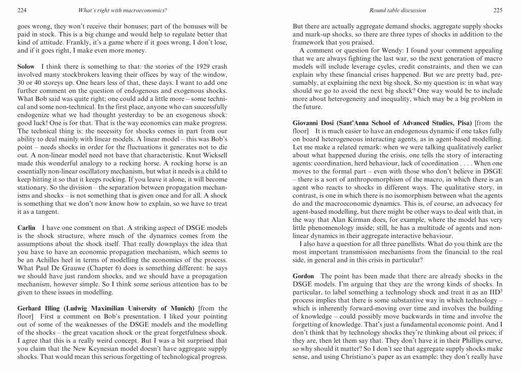
224 What’s right with macroeconomics?
goes wrong, they won’t receive their bonuses; part of the bonuses will be
paid in stock. This is a big change and would help to regulate better that
kind of attitude. Frankly, it’s a game where if it goes wrong, I don’t lose,
and if it goes right, I make even more money.
Solow I think there is something to that: the stories of the 1929 crash
involved many stockbrokers leaving their offices by way of the window,
30 or 40 storeys up. One hears less of that, these days. I want to add one
further comment on the question of endogenous and exogenous shocks.
What Bob said was quite right; one could add a little more – some techni-
cal and some non- technical. In the first place, anyone who can successfully
endogenize what we had thought yesterday to be an exogenous shock:
good luck! One is for that. That is the way economics can make progress.
The technical thing is: the necessity for shocks comes in part from our
ability to deal mainly with linear models. A linear model – this was Bob’s
point – needs shocks in order for the fluctuations it generates not to die
out. A non- linear model need not have that characteristic. Knut Wicksell
made this wonderful analogy to a rocking horse. A rocking horse is an
essentially non- linear oscillatory mechanism, but what it needs is a child to
keep hitting it so that it keeps rocking. If you leave it alone, it will become
stationary. So the division – the separation between propagation mechan-
isms and shocks – is not something that is given once and for all. A shock
is something that we don’t now know how to explain, so we have to treat
it as a tangent.
Carlin I have one comment on that. A striking aspect of DSGE models
is the shock structure, where much of the dynamics comes from the
assumptions about the shock itself. That really downplays the idea that
you have to have an economic propagation mechanism, which seems to
be an Achilles heel in terms of modelling the economics of the process.
What Paul De Grauwe (Chapter 6) does is something different: he says
we should have just random shocks, and we should have a propagation
mechanism, however simple. So I think some serious attention has to be
given to these issues in modelling.
Gerhard Illing (Ludwig Maximilian University of Munich) [from the
floor] First a comment on Bob’s presentation. I liked your pointing
out of some of the weaknesses of the DSGE models and the modelling
of the shocks – the great vacation shock or the great forgetfulness shock.
I agree that this is a really weird concept. But I was a bit surprised that
you claim that the New Keynesian model doesn’t have aggregate supply
shocks. That would mean this serious forgetting of technological progress.
M3014 - SOLOW TEXT.indd 224 21/11/2012 13:03
Round table discussion 225
But there are actually aggregate demand shocks, aggregate supply shocks
and mark- up shocks, so there are three types of shocks in addition to the
framework that you praised.
A comment or question for Wendy: I found your comment appealing
that we are always fighting the last war, so the next generation of macro
models will include leverage cycles, credit constraints, and then we can
explain why these financial crises happened. But we are pretty bad, pre-
sumably, at explaining the next big shock. So my question is: in what way
should we go to avoid the next big shock? One way would be to include
more about heterogeneity and inequality, which may be a big problem in
the future.
Giovanni Dosi (Sant’Anna School of Advanced Studies, Pisa) [from the
floor] It is much easier to have an endogenous dynamic if one takes fully
on board heterogeneous interacting agents, as in agent- based modelling.
Let me make a related remark: when we were talking qualitatively earlier
about what happened during the crisis, one tells the story of interacting
agents: coordination, herd behaviour, lack of coordination . . . . When one
moves to the formal part – even with those who don’t believe in DSGE
– there is a sort of anthropomorphism of the macro, in which there is an
agent who reacts to shocks in different ways. The qualitative story, in
contrast, is one in which there is no isomorphism between what the agents
do and the macroeconomic dynamics. This is, of course, an advocacy for
agent- based modelling, but there might be other ways to deal with that, in
the way that Alan Kirman does, for example, where the model has very
little phenomenology inside; still, he has a multitude of agents and non-
linear dynamics in their aggregate interactive behaviour.
I also have a question for all three panellists. What do you think are the
most important transmission mechanisms from the financial to the real
side, in general and in this crisis in particular?
Gordon The point has been made that there are already shocks in the
DSGE models. I’m arguing that they are the wrong kinds of shocks. In
particular, to label something a technology shock and treat it as an IID3
process implies that there is some substantive way in which technology –
which is inherently forward- moving over time and involves the building
of knowledge – could possibly move backwards in time and involve the
forgetting of knowledge. That’s just a fundamental economic point. And I
don’t think that by technology shocks they’re thinking about oil prices; if
they are, then let them say that. They don’t have it in their Phillips curve,
so why should it matter? So I don’t see that aggregate supply shocks make
sense, and using Christiano’s paper as an example: they don’t really have
M3014 - SOLOW TEXT.indd 225 21/11/2012 13:03
226 What’s right with macroeconomics?
any aggregate demand shocks except the Taylor Rule error term, and that
differs very significantly from the traditional paradigm that I offered,
where you get a shock even if the Fed is exactly carrying out the Taylor
Rule. If you have some source of inflation, you’re going to get higher
interest rates, and that’s going to potentially cause a recession, cause a
decline in aggregate demand, but it is not an error in the Taylor Rule; it
could be carrying out the Taylor Rule perfectly. And that brings us then
to this question of where are these transmission shocks from monetary
policy? And there we have traditional downward- sloping demand curves
for global goods with respect to interest rates; we have asset prices and
liabilities working through the Modigliani- type consumption function,
and then we have institutional arrangements that can lead to credit con-
straints. We’ve learned from the leverage cycle and from Wendy’s nice link
here that the collapse of an asset bubble automatically leads to increased
demand for collateral, which is partly the story of my mortgage broker
and one of the reasons why so many of his deals get turned down. So
we’ve got at least four channels there between financial markets and the
real economy.
Carlin Gerhard had a nice question on what we should be doing if we
are going to prepare ourselves for the next global crisis, and whether a
focus on heterogeneity and distribution is a core issue. One response is
rather like what Ricardo Caballero (2010) said in a recent article, where
he talked about the dangers of the pretence of knowledge in macroeco-
nomics. He argued that we should now be in broad exploratory mode
rather than in narrow fine- tuning mode. That captures what I think is
important. There has been a lot of new work on the Great Depression,
for example, and on Japan. These things are all enlightening, but do
they help us in a forward- looking way? I think we need to be working
in macroeconomics in the two following directions. One is bringing into
macroeconomics and properly taking account of the race between skills
and technology. This interaction between skills- biased technical progress
and the ability of the economy to generate human capital is very much at
the core of the inequality story, and it has macroeconomic consequences
that are not going to go away, irrespective of how we come out of this
crisis. That leads to the second point, which also touches on Giovanni’s
[Dosi] transmission mechanisms (see Chapter 5), which we’ve hardly
talked about at all, and that’s the question of really taking seriously what
it means when the dynamic of growth in the world economy shifts from
being driven by the advanced economies to being driven by China. It
relates to the recycling of surpluses – the point that came up earlier that
even though China has such an enormous investment share, it has an
M3014 - SOLOW TEXT.indd 226 21/11/2012 13:03
Round table discussion 227
even higher savings share, so that those surpluses have to be recycled. The
question of how that recycling takes place points the finger at the role of
the financial system, and whether the financial system is playing its role
in allocation or playing a role in generating another bubble. I don’t have
any special insight into what the next kind of crisis will be, of course, but
I think these are the core issues that macroeconomics has got to get to
grips with.
Gordon I’d like to talk about the next crisis. The potentially possible next
crisis is one that all of us would think of initially – the eurozone. If there
is enough contagion in the eurozone, starting in the periphery and moving
towards the centre, the problem could become too big for the body politic
in France and Germany to be willing to continue to finance. A crisis of
that kind could lead to the dissolving of the euro or some sort of perma-
nent recession or great depression in some of the countries that are most
vulnerable. In the case of the United States, I would worry most about a
long, slow erosion, closely related to Jean- Louis’s comment earlier about
the problems of his company in competing with the emerging markets and
how sophisticated they are getting in making all the stuff that used to be
the comparative advantage of the rich countries.
In my story, there are four causes of increased inequality in the United
States for the bottom 90 per cent. The four at the bottom are the decline
of the unions, the decline of minimum wage, and the globalization pair of
immigration and imports, which are very nicely characterized by Richard
Cooper in the Cournot Centre’s volume, The Shape of the Division of
Labour (2010). If you go back to Heckscher–Ohlin, you would predict that
globalization and the linking together of the Indian and Chinese labour
markets with the rich countries is going to inevitably push down the wages
of the low- skilled in the rich countries. On top of that, you’ve got these 14
million lost jobs in the United States, and everybody who is getting a job,
who was previously employed, most are taking enormous cuts in wages.
That is going to further cause measured inequality to rise, because you’re
going to have minimal, if not negative, income growth in the bottom 70,
80, 90 per cent of the income distribution. A possible outcome, which is
Ned Phelps’ current mantra, is that we can never get below 7 per cent
unemployment again; there are too many people in the workforce who
are going to lose their skills, almost like the insider/outsider story that
has been told about Europe for the last 20 years. This means a loss of
potential output and what happened in Europe starting in 1985: this long,
slow erosion meant that there was not enough capital stock, not enough
investment, to fully employ the people that used to be working at the peak.
If 14 million people aren’t working for ten years, some of the capital they
M3014 - SOLOW TEXT.indd 227 21/11/2012 13:03

228 What’s right with macroeconomics?
work with is going to depreciate, and there’s no incentive to replace it. So
you end up with lower potential output and a permanent slowdown in eco-
nomic growth. I see that kind of long, slow erosion, sort of Japanese- style
outcome, as more likely than the lightning bolt of a crisis.
NOTES
1. Works Progress Administration.
2. Civilian Conservation Corps.
3. Independent and identically distributed random variables.
REFERENCES
Blanchard, O. (2009), ‘The state of macro’, Annual Review of Economics, 1, 209–28.
Caballero, R.J. (2010), ‘Macroeconomics after the crisis: time to deal with the pretense- of- knowledge syndrome’, Journal of Economic Perspectives, 24(4), 85–102.
Christiano, L.J., M. Trabrandt and K. Walentin (2010), ‘Involuntary unemploy-ment and the business cycle’, Working Paper Series 238, Sveriges Riksbank (Central Bank of Sweden).
Cooper, R.N. (2010), ‘How integrated are Chinese and Indian labour into the world economy?’, in R.M. Solow and J- P. Touffut (eds), The Shape of the Division of Labour: Nations, Industries and Households, Cheltenham, UK and Northampton, MA, USA: Edward Elgar Publishing, pp. 101–21.
Friedman, Milton (1968), ‘The role of monetary policy’, American Economic Review, 58, 1–17.
Geanakoplos, J. (2009), ‘The leverage cycle’, NBER Macroeconomics Annual 2009, Vol. 24, Cambridge, MA: MIT Press, pp. 1–65.
Glyn, A. (2009), ‘Functional distribution and inequality’, in W. Salverda, B. Nolan and T. Smeeding (eds), The Oxford Handbook of Economic Inequality, Oxford: Oxford University Press, pp. 101–26.
Gordon, Robert J. (2011), ‘The history of the Phillips Curve: consensus and bifur-cation’, Economica, 78, January, 10–50.
Hicks, J.R. (1950), A Contribution to the Theory of the Trade Cycle, Oxford: Clarendon.
Kumhof, M. and R. Rancière, (2010), ‘Inequality, leverage and crises’, IMF Working Paper 10268.
Phelps, Edmund S. (1968), ‘Money- wage dynamics and labor- market equilibrium’, Journal of Political Economy, 76, 678–711.
Philippon, T. and A. Reshef (2009), ‘Wages and human capital in the US financial industry: 1909–2006’, NBER Working Paper 14644, January.
Rajan, R. (2010), Fault Lines, Princeton, NJ: Princeton University Press.Saez, E. and T. Piketty (2003), ‘Income inequality in the United States, 1913–
1998’, Quarterly Journal of Economics, 118(1), 1–39.
M3014 - SOLOW TEXT.indd 228 21/11/2012 13:03
Round table discussion 229
Shin, H. (2009), ‘Comment’ on Geanakoplos (2009) NBER Macroeconomics Annual 2009, 24, Cambridge, MA: MIT Press, pp. 75–84.
Woodward, Bob (2000), Maestro: Greenspan’s Fed and the American Boom, New York: Simon & Schuster.
M3014 - SOLOW TEXT.indd 229 21/11/2012 13:03