what is the probability you are a bayesian? · these two that illustrate bayesian inference using...

Journal of Statistics Education, Volume 22, Number 2 (2014)

1

What is the probability you are a Bayesian? Shaun S. Wulff Timothy J. Robinson University of Wyoming Journal of Statistics Education Volume 22, Number 2 (2014), www.amstat.org/publications/jse/v22n2/wulff.pdf Copyright © 2014 by Shaun S. Wulff and Timothy J. Robinson all rights reserved. This text may be freely shared among individuals, but it may not be republished in any medium without express written consent from the authors and advance notification of the editor. Key Words: Beta-Binomial; Conjugate prior; Prior specification; Subjective probability Abstract Bayesian methodology continues to be widely used in statistical applications. As a result, it is increasingly important to introduce students to Bayesian thinking at early stages in their mathematics and statistics education. While many students in upper level probability courses can recite the differences in the Frequentist and Bayesian inferential paradigms, these students often struggle using Bayesian methods when conducting data analysis. Specifically, students tend to struggle translating subjective belief to the specification of a prior distribution and the incorporation of uncertainty in the Bayesian inferential approach. The purpose of this paper is to present a hands-on activity involving the Beta-Binomial model to facilitate an intuitive understanding of the Bayesian approach through subjective problem formulation which lies at the heart of Bayesian statistics. 1. Introduction Carlin and Louis (2000, p. 1) state that, “The Bayesian approach to statistical design and analysis is emerging as an increasingly effective and practical alternative to the frequentist one.” Given the increasing popularity of the Bayesian approach to address statistical problems, it is important to expose students to this perspective. In particular, Stangl (1998) provides a nice discussion of some of the issues and challenges for incorporating the Bayesian paradigm into Statistics courses. It is especially important to provide students with meaningful applications and tangible experiences with Bayesian statistics to aid in the learning process. For example, Jessop (2010) presents a simple classroom activity demonstrating Bayesian inference in an introductory statistics course. Albert (2000) utilizes a sample survey project in an introductory course to introduce statistical inference from a Bayesian perspective. There are numerous references like


2

these two that illustrate Bayesian inference using the well-known Bayes’ Theorem for events (Casella and Berger 2002, p. 23). However, Bayes’ Theorem does not address the generality of the Bayesian approach that is based upon prior and posterior probability distributions which incorporate uncertainty on the parameters (Robert 2001, p. 9). Though not as common, classroom activities have been proposed to illustrate this more general Bayesian approach. Albert and Rossman (2009, Ch. 17) provide a number of problems for studying proportions using continuous probability distributions. Their examples are designed for students in an introductory statistics course who are familiar with basic probability concepts. Kern (2006) describes an entertaining application of Bayesian inference using the game Pass the Pigs® to model multinomial probabilities with the Dirichlet probability distribution. This class activity is designed for undergraduates and graduates majoring in mathematics and statistics. DiPietro (2004) uses a psychological therapy project to engage students with advanced Bayesian methodology such as posterior simulation, sensitivity analysis, and Bayes factors. This project is designed for first-year graduates in an applied Bayesian methods class that is computationally intensive. In light of the competing paradigms to statistical inference, many statisticians have been asked, “Are you a Bayesian or Frequentist?” Definitive answers to this question have led to acrimonious debates. A Frequentist is thought of as one who would address a particular statistical inference problem from a perspective which treats the observations as random (from hypothetical replications) and the parameter of interest as an unknown, fixed constant. A Bayesian would address a particular statistical inference problem by regarding the experimental outcome as fixed and treating the parameter of interest as random (reflecting uncertainty in knowledge about the parameter). In this case, the parameter has a probability distribution before the data is collected (prior distribution) and a probability distribution after the data is collected (posterior distribution). Many students in upper division undergraduate or beginning graduate courses in statistics have some familiarity with the Frequentist versus Bayesian debate, but they generally have not been trained in Bayesian statistics. Their background in statistical methodology has been almost exclusively from a Frequentist perspective. In this manuscript, we propose an assignment to engage the students in the Bayesian paradigm which leads them away from the ‘yes’ or ‘no’ dichotomy of being a Bayesian. We consider the question: What is the probability you are a Bayesian? We will henceforth denote this question as ‘Q.’ Since Q involves the concept of Bayesian statistics, it is necessary to consider what a Bayesian would do. Also, since Q is inherently subjective, it nicely facilitates the incorporation of a prior distribution. This question also recognizes that personal growth as a statistician is an ongoing process. What was posterior belief in an earlier experiment becomes prior belief in the next (Press 2003, p. 6). We pose Q to students in an upper-level statistical inference course (i.e., a mix of upper division undergraduate and first-year graduate students). Texts for such courses include Berry and Lindgren (1996), Bickel and Doksum (2001), Casella and Berger (2002), and Hogg, McKean, and Craig (2005). Students are expected to use a Bayesian approach to provide their personal answer to Q. Students are asked to provide a prior beta distribution to characterize their subjective belief about being a Bayesian. Next, each student is given a randomly selected inferential problem from a collection of problems appropriate to the particular class. For their problem, each student is expected to collect data and use that the data to conduct statistical inference utilizing either a Frequentist or Bayesian paradigm. The choice of either a Frequentist


3

or Bayesian approach for their randomly chosen problem is treated as a single observation from the Binomial (or Bernoulli) distribution with which they update their beta prior distribution on Q. The transition from prior to posterior distribution utilizes the Beta-Binomial model which is frequently the first model used in teaching Bayesian statistics. For convenience, Table 1 shows the complete assignment. Table 1. The assignment for the class exercise. Let ‘Q’ denote the following question: “What is the probability that you are a Bayesian?” You are to answer Q utilizing a Bayesian inferential approach. Please address the following in your write‐up. You have two weeks to complete this assignment.

A. Prior Specification: Let Q

denote the probability that you are a Bayesian. The first

step in conducting inference on Q is to assign a prior distribution. Assume

~ Beta ,Q a b where a and b are hyperparameters.

1. Specify a particular Beta distribution that you feel most accurately describes your affinity towards being a Bayesian. Justify why you chose this particular Beta distribution. A well explained graph could be highly beneficial. 2. Give the mean, variance, and quantiles (0.025, 0.25, 0.50, 0.75, 0.95) for your prior distribution.

B. Experiment: Conduct an experiment to estimate the true proportion ( ) of

‘successes’ for your randomly selected problem from the collection of N proportion

problems. Your experiment will consist of n independent trials where Y denotes the number of trials which results in a success.

1. Obtain a single random number from 1,..., N . Give that number to the instructor to

receive your randomly selected problem. Briefly describe the problem and any experience that you may have with your problem. 2. Carefully explain whether you used a Frequentist or Bayesian inferential approach for the problem in 1. Your discussion should involve the Bayesian characterizations (B1), (B2), (B3) or the Frequentist counterparts (F1), (F2), (F3). (These characterizations are given in Section 2.)

3. Briefly describe how you obtained the sample data for your problem. Be sure to report your sample size. What were your considerations in choosing the number of trials that you conducted? (This last question is required only for advanced classes.)


4

4. Report the number of successes, point estimate, uncertainty of your point estimate, and the 95% interval estimate for . Carefully interpret your interval estimate.

C. Posterior Distribution: For your scenario, let X take the value 1 if a Bayesian approach was used in B and 0 if a Frequentist approach was used in B. Then

~ Binomial 1,QX where there is a single experimental trial based upon X .

The posterior distribution of Q is obtained from your prior distribution in A and your

observed value of X x from B.

1. Give the posterior distribution based upon x . What is the mean, variance, and quantiles (0.025, 0.25, 0.50, 0.75, 0.975) for your posterior distribution? 2. Provide a plot of your posterior distribution for Q .

3. Describe what sort of change you observed between your prior and posterior

distributions on Q . In addition, calculate the absolute relative mean difference as

|prior mean ‐ posterior mean|/(posterior std dev). 4. Give your answer to Q. Include in your answer a description of your posterior

estimate and the posterior uncertainty of Q .

This manuscript consists of the following sections. Section 2 provides a description of student background in this upper-level course along with some of the issues we commonly encounter as students attempt to wrap their minds around the Bayesian inferential paradigm. Section 3 describes the class instruction prior to giving the assignment where we characterize the population of problems and provides specific insights into the Bayesian approach for this assignment. Sections 4, 5, and 6 provide details about the sections of the assignment including the prior distribution, the experiment, and the posterior distribution, respectively. These types of details arise in office hours and class discussions as students are working through the assignment. Guidance will be given in each of these sections for grading the assignment along with common errors. Example student scenarios will be used in each of these sections to illustrate the results of this project. Section 7 contains concluding remarks, points for class discussion, as well as feedback about the success of this assignment. 2. Background Since the intended course for this exercise is an upper-level undergraduate course in statistical inference, students are expected to have a background in probability theory and integral calculus. It is common to initiate the discussion of Bayesian statistics in the context of point estimation once Frequentist approaches (method of moments, maximum likelihood) have been discussed. Prior to going through this exercise, students have been exposed to in-class derivations of exact


5

posterior distributions for the Beta-Binomial model and the Normal-Normal model. When writing the expression ‘Distribution1-Distribution2,’ students understand that ‘Distribution1’ denotes the prior distribution while ‘Distribution2’ denotes the distribution of the population from which the data is sampled. The Beta-Binomial and Normal-Normal models are typically used in course texts (e.g., Casella and Berger 2002, pp. 324-326) to introduce the Bayesian approach since they are conjugate families in which the posterior distribution is from the same family of distributions as the prior distribution. Students have also been taught that there are three main distinctions which characterize the Bayesian approach:

(B1). The parameter of the population model is treated as a random variable. (B2). A prior distribution for the parameter is utilized. (B3). The inferential procedure is based upon the experimental outcome.

These distinctions are in opposition to the Frequentist approach in which: (F1) The parameter is treated as a fixed unknown constant; (F2) A prior distribution is not utilized; (F3) The inferential procedure is based upon a collection of outcomes which could occur in hypothetical replications of the experiment. While students can generally recite such differences between the two inferential paradigms, they often struggle making the transition to the Bayesian perspective when actually conducting statistical inference. Many of them need more than discussion points (B1), (B2), (B3) and a couple of mechanistic examples. This is the motivation behind the proposed exercise to answer Q. Experimental information is incorporated according to whether or not the student adopts a Bayesian approach [(B1), (B2), (B3)] or a Frequentist approach [(F1), (F2), (F3)] in drawing inference for their randomly selected problem. This assignment can be organized in several ways, but for the purpose of this manuscript, we present the exercise as a single homework assignment which students have two weeks to complete. Students are permitted to ask questions or seek clarifications about the assignment from the instructor. Once the assignment is completed and assessed, a class session is spent discussing results, challenges encountered, and understandings gained from the assignment. Through this exercise, students personally experience a variety of important steps in the Bayesian decision making paradigm. These experiences include: (a) translating subjective belief to the specification of a prior distribution; (b) carrying out a Bayesian analysis with their own data; and (c) incorporating uncertainty in the Bayesian inferential approach. 3. Insights into the Bayesian Approach for this Problem When the assignment in Table 1 has been handed out, students may feel overwhelmed asking, “Now what am I going to do?” It can be reassuring and instructional for the students to take class time to put the assignment in perspective and to remind them of some of the basic tenants of Bayesian inference. We first consider a population of problems P from which Q should be answered. Thus, the

answer to Q will be conditional on P. Let Q denote the proportion of problems in P in which

the student applies the Bayesian paradigm, or equivalently, the probability that the student is a Bayesian. Restrictions on P should include: 1. the student has the capability to carry out their


6

preferred paradigm for that problem and 2. the student is easily able to collect their own data for that problem. For our particular class, we further limit P to consist of a large collection of proportion problems. Not only do we do this to satisfy our two requirements above, but we also like to have students work with the Beta-Binomial model for both their experiment and for obtaining their answer to Q. This approach allows them to see the similarities and differences between the inferential approach they choose and the Bayesian approach required to answer Q. A course instructor using this assignment would not have to use the same set of proportion problems, or to even use proportion problems to formulate P. This population P may be quite large or even infinite. In order to make the assignment feasible,

we consider a set of N problems which defines a sampling frame containing a representative

collection of problems from P. For implementation of this assignment, our consists of 100N proportion problems involving binary outcomes associated with: 1. tossing objects (i.e.,

coin, checker, tack), 2. binary survey questions (i.e., credit card holder, smoker, cell phone user), and 3. binary object identifications (i.e., car color, gender, parent). Thus, each problem in has an associated storyline which varies in problem type, student familiarity with the problem, and the required sampling effort. These characteristics could affect whether a student thinks that a particular problem can best be analyzed from a Frequentist or Bayesian viewpoint. Thus, it is important to have a diverse collection of problems in in order to have variability with respect to these characteristics. For example, a student might think that for a survey type problem, such as assessing the probability a university student owns a credit card, it is better to treat the probability as random (B1). A student who must assess the probability that a local resident has children might be more inclined to incorporate prior information (B2) if they provide child care. A student who must assess the probability of heads for a coin toss might be less inclined to condition on the experimental outcome (B3) when it is easy to obtain numerous outcomes. A large collection of proportion problems can be developed using Albert and Rossman (2009), Dunn (2005), and Albert (2000). Students are reminded that the probability Q is represented as a random variable with

realizations, , which lie between 0 and 1. As such, there is uncertainty in Q . Students are also

reminded that uncertainty in the knowledge about Q is formally incorporated through a

probability density function (PDF). Before conducting an experiment, we consider the prior PDF, . The prior PDF for our

model is obtained from the Beta distribution, Beta ,Q a b (see Appendix A.2.1). This is a

convenient PDF for modeling probabilities since it has support over values from 0 to 1 and since it can have a variety of shapes according to the values of a and b (Albert and Rossman 2009, Ch. 17). The prior PDF is

11 1ba . (1)


7

Figure 1. Visual representation of sources of information about Q .

Suitable values for a and b need to be chosen to reflect one’s belief about Q . Subjective

knowledge about Q can come from many sources. Four possible sources are depicted in Figure

1 including background from past course instruction in Bayesian statistics, previous experience applying Bayesian methods, preference (popularity) for the Bayesian paradigm, and the ability or perceived ease of carrying out a Bayesian analysis. These four sources provide information about reasonable values for Q . These sources also provide uncertainty about Q since it is not known

how each one of them will impact the choice of paradigm when faced with a particular problem from the population P. As shown in Figure 1, knowledge about Q also comes from the current behavior observed in an

experiment. The experiment consists of the number of Bayesian inferential approaches (successes), X , adopted out of n inferential problems (trials). Thus, the experiment is modeled by the Binomial distribution, Binomial ,X n (see Appendix A.1.1). The knowledge from

the experiment is incorporated through the likelihood function which conveys information about likely values of Q as well as the uncertainty associated with the observed experimental result.

The likelihood function is given by

1n xxL x . (2)

While our development utilizes the Beta-Binomial model, it is important to remind students that their experiment represents only a single randomly chosen inferential problem, i.e. 1n . Plausible values for Q are reflected through both prior knowledge and the experimental result.

The information about Q from the prior PDF in (1) and the likelihood function in (2) are

combined via the posterior PDF, x . The posterior PDF is defined as (Casella and Berger

2002, p 324-325)


8

1

0

L xx

L x d

(3)

11

1 11

0

1

1

n x bx a

n x bx a d

11 1

,

n x bx a

B x a n x b

(4)

where the constant ,B x a n x b is the Beta function (see A.2.1). We also see from (4) that

the posterior PDF has the Beta distribution, Beta ,x x a b n x . Thus, the class of Beta

distributions is a conjugate family for the class of Binomial distributions since the resulting posterior distribution also has a Beta distribution with updated parameter values. For many students, the overview given above is illuminating in that they now see that the formula in (3) which they have been learning can incorporate both information and uncertainty from the prior distribution and the likelihood. At this point, students are generally able to think about the remaining challenges in the assignment. More specifically: 1. How do I specify my prior PDF? 2. How do I incorporate and interpret the uncertainty in the prior and posterior PDFs? 3. How do I describe the Bayesian or Frequentist approaches to inference when I conduct inference for the randomly chosen experiment? In order to give an idea of “typical student work” in this manuscript, we introduce three hypothetical students. These students represent three common combinations of the descriptions shown in Figure 1 based upon previous implementations of the assignment. Freddy Frequentist only has background and experience with Frequentist based statistics and has little preference for the Bayesian approach. Betty Bayesian has had positive experiences with the Bayesian approach in previous courses and with research projects which has influenced her preference for this paradigm and given her the ability to carry it out. Naive Ned has limited background and experience with both approaches and has no obvious preference for either paradigm. Thus, it is natural to expect these types of students to differ in their answers to Q. 4. Formulation of Prior Distributions Section A (questions A.1-A.2) of the assignment in Table 1 requires students to incorporate the prior information and uncertainty concerning Q utilizing the Beta PDF in (1). We have found

that it takes skill to convert a priori scientific information into a probabilistic distribution. Consequently, students are reminded in class of familiar facts concerning the Beta distribution and how to use those facts to choose their prior. Students are encouraged to explore their choice of a and b graphically by altering these values and observing how the Beta distribution changes. We have also found it beneficial to require students to give the mean, standard deviation and quantiles of their prior distribution. Taking the time to reflect on the meanings of these distributional summaries helps the student strengthen their argument for why they chose the particular values of a and b. More specifically, if Beta ,Q a b where a and b are

hyperparameters, then the mean and variance of Q are given by


9

EQ Q

ae

a b

and E 1 E

V1

Q Q

Q Qva b

, (5)

respectively (see A.2.1). Thus, a can be chosen relative to b so that the mean of the distribution reflects the prior estimate of being a Bayesian. At this point, one could also bring up the notion that the effective sample size for the Beta prior is a b (Morita et al. 2008). As such, a b could be understood to represent the number of hypothetical inferential problems out of which a of those problems are addressed via a Bayesian approach. Students can also see from (5) that when this effective sample size a b is large,

then the variability of the prior distribution is small. Rather than having students guess the values of a and b, it is possible to select these values so as to obtain mean Qe and uncertainty Qv using

211Q Q Q Q

Q

a e e e vv

, 1 QQ

ab e

e . (6)

Specification of hyperparameters can also be discussed with students for commonly used priors to provide additional insights. A vague prior distribution is dispersed over the unit interval with small a b while an informative prior distribution is concentrated with large a b . If a b , then the PDF is symmetric about 0.5. A uniform prior has 1a b and Jeffreys prior has

0.5a b (Robert 2001, pp. 129-130). Zhu and Lu (2004) consider the least influential prior with 0a b . However, this prior is improper as it does not integrate to 1. This prior can be approximated using the common trick of choosing a and b to be close to 0. Examples of the prior PDFs for our three students (i.e. Freddy Frequentist, Betty Bayesian, Naive Ned) are plotted in Figure 2 and distributional characteristics are provided in Table 2. Table 2. Summaries of the prior distributions for the three types of students including values of the hyperparameters (a, b), mean ( Qe ), standard deviation ( 0 5

Qv . ), and quantiles (q).

Name a b Qe 0 5Qv .

0 025q . 0 25q . 0 50q . 0 75q . 0 975q .

Frequentist Fred 1 9 0.10 0.091 0.003 0.032 0.074 0.143 0.336 Betty Bayesian 3 1 0.75 0.193 0.292 0.630 0.794 0.909 0.992 Naive Ned 1 1 0.50 0.289 0.025 0.250 0.500 0.750 0.975


10

Figure 2. Prior distributions for Freddy Frequentist, Betty Bayesian, and Naive Ned.

Table 2 shows that when Freddy Frequentist is presented with the population of problems P that on average he would use a Bayesian approach in 1 out of 10 of these problems and no more than 4 out of 10 of these problems (prior probability less than 0.025). In light of (5), 1/10 0.1Qe

and 0.1(0.9) /11 0.09Qv . Along with the “black” profile in Figure 2 and the first line of

Table 2, Freddy Frequentist might also provide the following explanation for his choice of prior:

“My prior is specified to demonstrate a high probability of using a Frequentist approach with a fair amount of certainty. That is, I imagine I would only use a Bayesian approach in 1 out of 10 inferential problems. Thus, I chose my prior mean for being Bayesian as 0.1 with uncertainty less than 0.1. In fact, there is greater than 50% chance that my probability of being Bayesian will be between 0.03 and 0.15.”

Once a Beta prior has been specified, values such as those in Table 2 are rather simple to obtain to answer A.2. Thus, the grading of A.2 merely involves checking if these summaries match the specified distribution. Generally, students perform well on this part. On the other hand, A.1 is one of the most challenging and important questions on the assignment. The grader must ascertain whether or not the specified Beta prior matches the one the student intended. Prior justification is critical in this assessment; just as it is in any Bayesian analysis. Thus, it is not surprising that students struggle with this question. We have found that plotting various Beta PDFs, thinking about the numerical summaries in (5), briefly exploring effective sample size, and going over some of the commonly used Beta priors helps to prepare students to adequately justify their prior distribution. 5. A Simple Experiment Section B of the assignment requires each student to conduct an experiment for their randomly selected problem so that they have data to inform their answer to Q. In this section, and for the remainder of the manuscript, we will refer to the four questions in Section B of the assignment in


11

Table 1 as B.1-B.4. Our population P consists of proportion problems. Each of these problems are modeled with the Binomial distribution where we let Y denote the number of trials out of n that results in a success and we let denote the true probability of success. Assuming independent trials, then Binomial ,Y n .

Question B.1 asks students to randomly generate a number of from 1,..., N which can be done using computer programs. For our student examples, we will assume that Freddy Frequentist draws a problem in which he must assess the probability that a common thumbtack lands point up (thumbtack experiment). Betty Bayesian draws a problem in which she must assess the probability that a local resident has children (child experiment). Naive Ned draws a problem in which he must assess the probability that a car on a major city street contains a passenger talking on a cell phone (cell phone experiment). Question B.2 asks students to explain whether or not they used a Frequentist or Bayesian inferential approach when conducting inference for their problem. Students should address points (B1), (B2), (B3) from Section 2. Formulas that students might use are provided in the Appendix for convenience for the Frequentist approach (A.1) and for the Bayesian approach (A.2). It is helpful for students to clearly address their inferential approach here as this will dictate their answers to questions B.3 and B.4. Question B.3 asks students to justify a selected value for the number of trials, n, for their randomly selected problem. Sample size selection can be tricky due to its connections with the inference procedure. For example, large sample sizes allow for normal approximations for the Frequentist approach (A.1.3) and for the Bayesian approach (A.2.3). Large sample sizes also decrease the influence of prior information (Press 2003, p. 174) (see A.2.2). While sample size calculation is not a main objective of the assignment, students find it to be a hurdle in carrying out their experiment. The most common question on the assignment is, “What sample size should I use?” For introductory classes, B.3 is not required and the instructor can specify the number of trials (such as 10, 15, or 20). However, we encourage students in advanced classes to think about sample size selection since it is fundamental to experimentation. One approach is to select a sample size so that the uncertainty is below a threshold (see A.1.2, A.2.2). Sample size can also be chosen so that normal approximations hold or to have particular weight on the prior mean (see A.1.3, A.2.2, A.2.3). Question B.4 asks students to provide a brief summary of their experimental results including the number of successes, point estimate, uncertainty, and a 95% interval estimate for . Answers to this question are provided in Table 3 for our student examples Freddy Frequentist, Betty Bayesian, and Naive Ned. Freddy used a Frequentist approach for the tack experiment and Ned used a Frequentist approach for the cell phone experiment. They calculated their estimate ˆ y n by evaluating the maximum likelihood or method of moments estimator using their

values of n and y (see A.1.2). Their measure of uncertainty corresponds to the estimated standard error (see A.1.3). They found 95% confidence intervals which would capture the true fixed value of in over 95% of the samples. Freddy obtained samples for his experiment by tossing the tack. It was easy for him to perform a large number of tosses, so he was able to use the large sample confidence interval (see A.1.4). Ned picked a moderately busy street in town and


12

systematically sampled 20 cars to determine how many drivers were talking on cell phones. Ned chose his sample size to be moderately large so that the associated uncertainty would be no larger than 0.125. Not wanting to rely on large sample assumptions, he computed a 95% confidence interval appropriate for a small number of trials (see A.1.4). Betty conducted a Bayesian approach for the child experiment. She specified a Beta prior distribution with 1.5a and 2.5b as she explains in her answer below. She randomly selected 10 houses and found that 4 residents indicated they had at least one child. She used her observed values of n and y to update the Beta prior to obtain the Beta posterior distribution as in (4). Her measure of posterior uncertainty is the posterior standard deviation (see A.2.2). She also computed a 95% credible interval using the highest posterior density (HPD) region (see A.2.4). Table 3. Answers to question B.4 for the three types of students which includes values of the

number of trials (n), number of successes (y), estimate of , uncertainty associated with the

estimate ˆu , and a 95% interval for .

Name n y ˆu 95% interval for

Frequentist Fred 50 24 0.480 0.071 0.342 0.538 Betty Bayesian 10 4 0.367 0.120 0.141 0.602 Naive Ned 20 4 0.200 0.089 0.050 0.400

For illustrative purposes, we also include answers to (B.1) (B.2), (B.3), (B.4) for Betty Bayesian.

(B.1) “My randomly selected problem is to assess the probability that a local resident has children. Thus, I plan to sample residences (by address) within a mile radius of my own. I am interested in this problem given that I enjoy babysitting to earn money.” (B.2) “I used a Bayesian approach to assess the probability that a local homeowner has children in order to incorporate my knowledge of the nearby residences. Thus, I let denote this probability which I am treating as random to recognize the uncertainty I have regarding its value (B1). I chose a conjugate beta prior distribution to incorporate my knowledge concerning . Since I babysit and I have lived in this area for awhile, I wanted to specify a moderately informative prior. Based upon my knowledge, I expect the probability to be about 0.3 with a standard deviation less than 0.2. Thus, I chose the hyperparameters a and b to achieve this expected value and standard deviation (see equation (5)). From the results of my particular experiment (B3), I observed 4 out of 10 residences which had at least one child. These results produced the posterior distribution for of Beta(5.5, 9.5) (see equation (4)). I plotted my prior and posterior PDFs (see Figure 3).” (B.3) “As mentioned in (B.2), I wanted to incorporate my prior information into this problem. I also wanted to have a small sample size since I would have to meet with people at the randomly sampled residences. Thus, it seemed to me that I could best achieve these two objectives with a sample size of 10 which places weight


13

1

3

a b

n a b

on my prior mean (see A.2.1). This sample size also maintains an

uncertainty or posterior standard deviation no larger than 0.13 (see A.2.1).” (B.4) “My figure (see Figure 3) shows the plot of my prior and posterior distributions for . The plot includes labels for my posterior estimate which corresponds to the posterior mean value 0.3 / 3 2 0.4 / 3 0.3667 (see A.2.2) so

that the posterior mean is slightly higher than the prior mean. The plot also shows the 95% HPD credible interval for which is the shortest interval containing 95% of the posterior probability. Thus, there is 95% posterior probability that is between 0.141 and 0.602. Uncertainty is assessed using the standard deviation of the posterior

distribution which has the value 0.50.3667 1 0.3667

0.12051.5 3.5 10 1

(see A.2.1). The

posterior uncertainty is less than the prior uncertainty due to observing 10 residences. The point estimate of 0.3667 seems to closely agree with my prior estimate. I could incorporate this knowledge in a future experiment using a more concentrated prior."

Figure 3. The prior and posterior distributions for Betty Bayesian in the child experiment.

Section B of the assignment contains challenging questions as students are expected to carry out an experiment and interpret the results. The grading of B.1 simply involves checking that the students have their scenario picked out and have adequately provided a brief description of it. Question B.2 may be the most difficult on the assignment. For this reason, we ask students to focus on addressing (B1), (B2), (B3) (or (F1), (F2), (F3)) in their written explanation. This guidance has improved student answers and causes them to focus on the critical distinctions between the two paradigms. The structure also helps the grader to better assess student understanding of this distinction. The assessment of question B.3 depends upon guidelines set by the instructor. This flexibility is necessary given differences between course levels. In advanced courses, we have found it helpful to utilize sample size guidelines (see A.1.2, A.1.3, A.2.2, A.2.3). The grader can then assess whether or not the students have adequately utilized those


14

guidelines. Students typically do well reporting the results from their experiment. However, some students struggle to correctly interpret their interval estimate in light of their chosen paradigm. Thus, the grader should be aware of such interpretation problems. Instructors also may wish to spend class time reviewing the interpretation of inferential results in light of the characterizations (B1), (B2), and (B3). These skills are crucial to the practicing statistician. 6. The Posterior Distribution The next portion of the assignment (part C and subsequently questions C.1-C.4) involves determining the posterior distribution of Q . The data from the experiment utilized to update the

prior on Q is based upon a single Bernoulli trial where 1n . The value from the trial is 1x

if a Bayesian approach is used to conduct inference for the randomly selected problem and 0x if a Frequentist approach is used to conduct inference for the randomly selected problem. The PDF, x , is the PDF of the Beta ,1x a x b distribution using (4). For instance, if a

Bayesian approach was utilized in the experiment, then 1x and the posterior distribution is

Beta 1,a b , and if a Frequentist approach was utilized, then 0x and the posterior

distribution is Beta , 1a b . The usual Bayes estimate is the posterior mean (see A.2.2)

1ˆ

1 1 1Q

a a b x ax

a b a b a b a b

. (7)

The posterior mean is a weighted average of the prior mean and the maximum likelihood

estimator with weight 1

a bw

a b

given to the prior mean. The uncertainty in the Bayes

estimate corresponds to the standard deviation of the posterior distribution (see A.2.2). Questions C.1, C.2, and C.3 from Table 1 involve summarizing aspects of the posterior distribution. We once again consider answers to these questions for Freddy Frequentist, Betty Bayesian, and Naive Ned. Table 4 gives summaries of the corresponding posterior distributions for C.1. Figure 4 gives the plot of the posterior distributions requested by C.2. The plots of the posterior PDFs in Figure 4 can be compared to the prior PDFs in Figure 2. Table 4. Summaries of the posterior distributions for the three types of students which includes the hyperparameters (a, b), value from the experiment (x), prior weight (w), mean

( Qe ), standard deviation ( 0 5Qv . ), and quantiles (q).

Name a b x w Qe 0 5Qv . 0 025q . 0 25q . 0 50q . 0 75q . 0 975q .

Frequentist Fred 1 9 0 0.909 0.091 0.083 0.003 0.028 0.067 0.129 0.309Betty Bayesian 3 1 1 0.800 0.800 0.163 0.398 0.707 0.841 0.931 0.994

Naive Ned 1 1 0 0.667 0.333 0.236 0.013 0.134 0.293 0.500 0.842


15

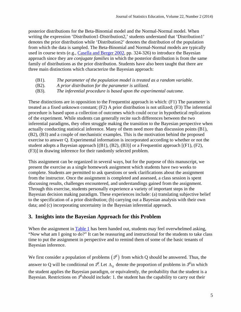
Figure 4. Posterior distributions for Freddy Frequentist, Betty Bayesian, and Naive Ned.

The spread of the distributions in Figure 4 illustrate the uncertainty contained in the posterior distribution. As each student plots their own posterior distribution, they can observe that the degree of uncertainty in the posterior can be summarized by the 95% equal tailed credible interval, 0.025 0.975,q q . For the three student examples, these credible intervals are provided in

Table 4. Highest posterior density intervals could also be calculated (see A.2.4). Question C.3 asks students to describe the change in the prior and posterior distributions using the absolute relative mean difference, given by

prior mean posterior mean

posterior std.dev.

. (8)

Equation (8) measures the change from prior mean to posterior mean relative to the posterior uncertainty. For our hypothetical students, the difference is most pronounced for Ned and least for Fred. This relative change is 11% for Freddy Frequentist, 31% for Betty Bayesian, and 71% for Naive Ned. An example of an answer to C.4 is given below from the perspective of Naive Ned.

“Based upon my vague prior with 1a and 1b , and the result of my experiment in which I used a Frequentist analysis so that 0x , my posterior distribution for the probability of being a Bayesian is Beta 1,2 . This means my posterior estimate of

this probability is 0.333 and a 95% credible interval based upon the percentiles is (0.013, 0.842). The 95% credible interval means that there is a 95% chance that my probability lays between these endpoints. Thus, there is a large amount of uncertainty in my answer to Q. However, this is not surprising given my vague prior and what I learned from conducting a single experiment. Nevertheless, the result from this experiment has refined my answer to Q given that my prior estimate was


16

larger with a value 0.500 and my 95% prior percentile interval was wider with values (0.025, 0.975) (see Table 2).”

Questions C.1, C.2, and C.3 utilize summaries based upon the posterior distribution. Question C.3 requires a summary involving both the prior and posterior distribution. Evaluation of these questions involves checking that the summaries are correct for the given posterior distributions. Students generally do well on these questions. The key part is C.4 where the student is asked to answer the ultimate question Q. A complete answer to this question involves the interpretation of the posterior distribution and how it pulls together prior information and the experimental result. This is a daunting task for the student, especially one being introduced to a Bayesian perspective. Yet, this is the purpose behind the assignment. Thus, the grader needs to assess if the student has adequately extracted the information and characterized the uncertainty from the posterior distribution to provide a practical answer to Q. An example of an adequate answer is provided above by Ned. A poor answer would be one in which summaries of the posterior distribution are merely reported without an accurate interpretation of these summaries or a description of how these summaries were obtained in light of the prior specification and the experimental result. Students are aided in this process through the individual questions in parts A, B, and C which break down their answer into smaller parts. As a result, question C.4 requires a short summary of the Bayesian approach that led to their answer to Q. 7. Conclusions The purpose of the proposed exercise is for students to gain personal experience with the Bayesian paradigm. We have found that students struggle making the transition from the mechanical presentation of Bayes Theorem to practical implementation of the Bayesian paradigm. These challenges include defining prior distributions, understanding differences between Frequentist and Bayesian approaches to statistics, the rationale behind extending Bayes theorem to incorporate uncertainty, and the commonly held view that one has to be either a Frequentist or a Bayesian. This assignment attempts to address each of these difficulties. Thus, it can be quite helpful to spend a large portion of a class period to reflect upon these challenges. As mentioned by Robert (2001, p. 106), specification of the prior distribution is the most important, and perhaps the most difficult aspect of the Bayesian analysis. Thus, it is not surprising to find that many students say that while they have information for their prior distribution, they have a hard time quantifying and characterizing that information. Plots of the student prior distributions are shown in class. Relating the uncertainty in the prior to student background, experience, preference, and simplicity as in Figure 1 aids in student understanding when it comes to prior specification. Discussions regarding informative and non-informative priors naturally come up. Students could also be asked to think of ways to specify a prior for a client. For example, it might be convenient to have the client think about the expectation, or balance point, of their prior distribution, along with their assessment of prior uncertainty. These values can then be put in equation (6) to obtain the hyperparameters. Plots of prior distributions could then be shown to the client. In addition, it may be helpful for the client to specify the mode and percentile of the prior distribution as in Branscum, Gardner, and Johnson (2005). Uncertainty concerning the hyperparameters a and b can also be accommodated using a hierarchical model (Robert 2001, p. 143) whereby prior distributions are assigned to the


17

hyperparameters. An empirical Bayes approach is another alternative where the hyperparameters are estimated by applying Frequentist methods to the marginal distribution

m x L y d (Press 2003, p. 212).

The second challenge is for students to understand differences between the Frequentist and Bayesian approaches. Thus, the class is informed of the number of students who used a Bayesian approach in their experiment which is typically less than one-third for these proportion problems. According to (A.2.2), the posterior mean is

Ea a b y n

ya b n a b n n a b

. (9)

The sample size n can be pre-selected to produce specific weights on the prior mean as a and b are known a priori. We see that for large n , relative to a and b, the weight on the sample mean is large. Equation (9) also shows that the Frequentist answer can be obtained with an improper prior with 0a b for any n while an approximate Frequentist answer is obtained when a and b are small relative to n . While these two approaches to statistical inference differ in interpretation and philosophy, they do not necessarily differ in terms of answers. Thus, it is important when expressing the differences between the Bayesian and Frequentist paradigms to focus on the Bayesian characterizations (B1), (B2), and (B3). It can also help students to hear some of the better answers to question B.2 during the class discussion. The third challenge refers to the incorporation of uncertainty in Bayes theorem. Plots can be shown of student posterior distributions and compared to the prior distributions. These probability density functions illustrate a students’ answer to Q both in terms of the mean and in terms of the uncertainty. Many students express surprise by how little their posterior distribution changes from their prior distribution. This provides a good opportunity to point out the amount of information these students have given to their prior distributions (effective sample size) relative to the single Bernoulli trial from the tack experiment. These students can also be reminded of their ongoing growth as statisticians. While it might be expected that the uncertainty in their prior distribution will decrease with added experience, background, and ability, the opposite may be true for many statisticians whose preference can vary widely between inferential problems. Students are reminded that for conjugate families, it is not too difficult to mathematically incorporate uncertainty through the posterior PDF as shown in Section 3. This is because the required integration in (3) is rather straightforward and the posterior distribution can be obtained simply by updating the hyperparameters of the prior distribution by the experimental result. In cases outside of conjugate families, it may not be so trivial to obtain the posterior PDF. In these cases, numerical techniques are needed to solve integration(s) like those in (3). These points provide a nice way to introduce students to popular computational techniques such as numerical integration, Monte Carlo methods, and Markov Chain Monte Carlo methods (Metropolis-Hastings, Gibbs Sampling) (Robert 2001, Ch. 6). These advanced computational methods are merely a tool to implement the Bayesian approach. This assignment arose out of the perceived need for students to gain practical experience using the extended form of Bayes Theorem in (3) by the instructor of this statistical inference course.


18

In this particular course, other inference topics are later discussed from the Bayesian framework including hypothesis testing, interval estimation, and prediction. Admittedly, students do not need this assignment to carry out the mathematical details required for these topics. However, students who have completed the assignment are more likely to ask about specifying the priors for these inference procedures and can more easily interpret Bayesian results. This is especially true for those students who have a low probability of being Bayesian. While these students may not have a preference for Bayesian methodology, the assignment provides them with some background, experience, and ability to carry out this approach. Thus, the students who have been trained mostly in Frequentist methodology are better prepared to comprehend and to utilize Bayesian concepts. The instructor has also noticed that it is easier for students who have completed the assignment to utilize Bayesian methods, including applications in consulting, research, and in other advanced statistical methods courses. Many students tend to see the assignment as challenging, so it is important to remind them of the practical experience they have gained from this assignment. It is also helpful to refer students back to this assignment when additional Bayesian topics are discussed later in the course.


19

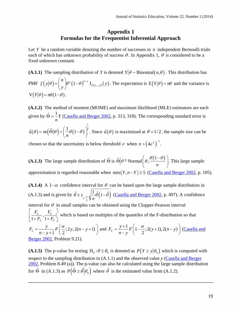
Appendix 1 Formulas for the Frequentist Inferential Approach

Let Y be a random variable denoting the number of successes in n independent Bernoulli trials each of which has unknown probability of success . In Appendix 1, is considered to be a fixed unknown constant. (A.1.1) The sampling distribution of Y is denoted Binomial ,Y n . This distribution has

PMF {0,1,..., }1n yy

n

nf y I y

y

. The expectation is E Y n and the variance is

V 1Y n .

(A.1.2) The method of moment (MOME) and maximum likelihood (MLE) estimators are each

given by 1ˆ Yn

(Casella and Berger 2002, p. 313, 318). The corresponding standard error is

u 1

21ˆse 1n

. Since u is maximized at 1/ 2 , the sample size can be

chosen so that the uncertainty is below threshold when 124n

.

(A.1.3) The large sample distribution of is 1ˆ Normal ,~

n

● . This large sample

approximation is regarded reasonable when min , 5Y n Y (Casella and Berger 2002, p. 105).

(A.1.4) A 1 confidence interval for can be based upon the large sample distribution in

(A.1.3) and is given by 1

2

1ˆ ˆ ˆ1zn

(Casella and Berger 2002, p. 497). A confidence

interval for in small samples can be obtained using the Clopper-Pearson interval

,1 1

UL

L U

FF

F F

which is based on multiples of the quantiles of the F-distribution so that

;2 , 2( 1)1 2L

yF F y n y

n y

and

11 ;2( 1), 2( )

2U

yF F y n y

n y

(Casella and

Berger 2002, Problem 9.21). (A.1.5) The p-value for testing 0 0H : is denoted as 0P Y y which is computed with

respect to the sampling distribution in (A.1.1) and the observed value y (Casella and Berger 2002, Problem 8.49 (a)). The p-value can also be calculated using the large sample distribution

for in (A.1.3) as 0ˆˆP where is the estimated value from (A.1.2).


20

Appendix 2 Formulas for the Bayesian Inferential Approach

Consider the scenario described in Appendix 1. In Appendix 2, let denote the random variable for the true probability of a success.

(A.2.1) Suppose Beta ,a b which has PDF 1 11(0,1)B , 1

baa b I where

B ,a b is the beta function given by

1 11

0B , 1

baa ba b d

a b

. The expectation

is Ea

a b

and the variance is

2V1

ab

a b a b

E 1 E

1a b

.

(A.2.2) The Bayes estimate (under squared error loss) is the expected value of the posterior distribution in (4) or E y (Casella and Berger 2002, p. 325). Using (A.2.1) and (A.2.2), the

posterior mean is Ea a b y n

ya b n a b n n a b

which is a weighted average of the

prior mean and the maximum likelihood estimate of in (A.1.3). A measure of uncertainty is taken to be the standard deviation of the posterior distribution in (3). By (A.2.1), this is u y

0.5

2 2

1sd |

1

ny a n y by

n a b n a b

. The uncertainty can be shown to be maximized at

* / 2y n b a n . The sample size can be chosen so that the uncertainty is below threshold

when 121 4n a b

.

(A.2.3) From Press (2003, p. 173), the large sample posterior distribution for a parameter is

1ˆ ˆ ˆ| Normal , J where

2

2

ˆ

ˆ lnJ L y

. For the Binomial model, is

given in (A.1.2) and ˆ

ˆ ˆ1

nJ

.

(A.2.4) A credible interval is of the form L U,C C such that L U 1P C C y . For an

equal tails credible interval, L / 2C B and U 1 / 2C B where B is the quantile of the

distribution in (4) which depends upon y, n, a, and b. For finding the highest posterior density (HPD) region, LC and UC must satisfy L UC y C y when the mode of the posterior

distribution lies in 0,1 , L 0C and U 1C B when the mode is 0 , LC B and U 1C when

the mode is 1 (Casella and Berger 2002, pp. 441-442). A credible interval can also be calculated


21

using the large sample posterior distribution in (A.2.3) which is the same as the large sample interval in (A.1.4). (A.2.5) The posterior probability for testing 0 0H : is denoted 0P y which is

computed by integrating the posterior PDF or evaluating the corresponding Beta CDF (Casella and Berger 2002, p. 379). This probability can also be evaluated using the large sample posterior distribution in (A.2.3). Acknowledgements This research was supported in part by a Basic Research Grant from the College of Arts and Sciences at the University of Wyoming in Laramie, Wyoming. The authors would like to thank the Editor, Associate Editor, and two anonymous referees for their thorough reading of the manuscript and their thoughtful comments and suggestions which have led to substantial improvements. References Albert, J. (2000), “Using a Sample Survey Project to Assess the Teaching of Statistical Inference,” Journal of Statistics Education [Online], 8(1). Available at http://www.amstat.org/publications/jse/secure/v8n1/albert.cfm Albert, J., and Rossman, A.J. (2009), Workshop Statistics: Discovery with Data, A Bayesian Approach, New York, NY: Key College Publishing. Berry, D.A., and Lindgren, B.W. (1996), Statistics: Theory and Methods (2nd ed.), Belmont, CA: Duxbury. Bickel, P.J., and Doksum, K.A. (2001), Mathematical Statistics (Vol. 1, 2nd ed.), Upper Saddle River, NJ: Prentice Hall. Branscum, A.J., Gardner, I.A., and Johnson W.O. (2005), “Estimation of Diagnostic-Test Sensitivity and Specificity through Bayesian Methodology,” Preventive Veterinary Medicine, 68, 145-163. Carlin, B.P., and Louis, T.L. (2000). Bayes and Empirical Bayes Methods for Data Analysis (2nd ed.), New York, NY: Chapman and Hall. Casella, G., and Berger, R.L. (2002), Statistical Inference (2nd ed.), Pacific Grove, CA: Duxbury. DiPietro, M. (2004), "Bayesian Randomized Response as a Class Project," American Statistician, 58(4), 303-309.


22

Dunn, P.K. (2005), “We Can Still Learn about Probability by Rolling Dice and Tossing Coins,” Teaching Statistics, 27(2), 37-41. Hogg, R.V., McKean, J.W., and Craig, A.T. (2005), Introduction to Mathematical Statistics (6th ed.), Upper Saddle River, NJ: Prentice Hall. Jessop, A. (2010), “Bayes Ice-Breaker,” Teaching Statistics, 32(1), 13-16. Kern, J.C. (2006), “Pig Data and Bayesian Inference on Multinomial Probabilities,” Journal of Statistics Education [Online],14(3). Available at http://www.amstat.org/publications/jse/v14n3 /datasets.kern.html Morita, S., Thall, P.F., and Müller, P.M. (2008), “Determining the Effective Sample Size of a Parametric Prior,” Biometrics, 64(2), 595-602. Press, S.J. (2003), Subjective and Objective Bayesian Statistics (2nd ed.), New York, NY: Wiley. Robert, C.P. (2001), The Bayesian Choice (2nd ed.), New York, NY: Springer. Stangl, D.K. (1998), “Classical and Bayesian Paradigms: Can We Teach Both?,” in Proceedings of the Fifth International Conference on Teaching Statistics, eds. L. Pereira-Mendoza, L.S. Kea, T.W. Kee, and W. Wong, vol. 1(1998), 251-258, International Statistical Institute. Zhu, M., and Lu A.Y. (2004), “The Counter-intuitive Non-informative Prior for the Bernoulli Family,” Journal of Statistics Education [Online],12(2). Available at http://www.amstat.org/publications/jse/v12n2/zhu.pdf Shaun S. Wulff Department of Statistics University of Wyoming 1000 E. University Ave. Laramie, WY 82071-3332 [email protected] Timothy J. Robinson Department of Statistics University of Wyoming 1000 E. University Ave. Laramie, WY 82071-3332 [email protected]

what is the probability you are a bayesian? · these two that illustrate bayesian inference using...

Documents