1

What is Q?

€

A = A0e−bt = A0e

−ω0t /(2Q )

Interpretation 1: Suppose A0 represents wave amplitudes, then

€

ln(A) = ln(A0) −ω0

2Q

⎡

⎣ ⎢ ⎤

⎦ ⎥t

slopeintercept

ln(A)

t

Interpretation 2: Suppose u represents displacement, then

€

u(t) = A0ei(a +ib )t = A0e

iω0teω0t /(2Q )

€

a = ω0 1−1/4Q2 (real)

€

b =ω0

2Q (imaginary)

=“modified” or “instantaneous freq”

Suppose: small attenuation, the

€

a ≈ ω ≈ ω0

€

b ≈ω

2QWe can define b = *, where * ---> 0 as Q increases (imaginary freq due to attenuation),

2

€

Q−1 = 2ω * /ω

€

* =ω

2QRelation with velocity:

€

c + ic* =ω

k+ i

ω *

k=

ω

k+ i

Q−1

2kImaginary velocity due to attenuation

€

c* =ω

2kQ−1 ⇒ Q−1 = 2

c *

cSo Q is a quantity that defines the relationship between real and imaginary frequency (or velocity) under the influence of attenuation.

Interpretation 3: Q is the number of cycles the oscillations take to decay to a certain amplitude level.

€

n = t /T = t(ω /2π )

€

then n ≈ t ω0/2π( ) → tn =n ⋅2π

ω0

€

if Q → ∞

So amplitude at time tn (after n cycles)

€

A(tn ) ≈ A0e−w0tn / 2Q = A0e

−w0n 2π /(ω0 2Q ) = A0e−nπ /Q

3

Attenuation and Physical Dispersion (continued…)

Different interpretations of Q (quality factor):(1)As a damping term Q = /(2)As a fraction between imaginary and real frequencies (or imaginary velocity to real velocity)

(3)As the number of cycles for a wave to decay to a certain amplitude. If n = Q, then

(4)Connection with t* (for body wave).

(5)Energy formula

€

Q−1 =2ω *

ω or Q -1=

2c *

c

€

A(tn ) = A0e−ω0t / 2Q = A0e

−(ω0 / 2Q )(n*2π /ω0 ) ≈ 0.04A0

€

t* =dt

Q(r)path

∫ ≈Δt i

Qii=1

N

∑ (N layers, r = location)

€

1

Q(ω)= −

ΔE

2πE (-ΔE = energy loss per cycle)

1 number that describes Q structure of several layers

Effects of Q (assume the SAME Q value)

€

(1) A(ω) = A0(ω)e−ω0t / 2Q ≈ A0(ω)e−ωx /(2Qv )

€

large distance x - - - - > more amplitude decay

large velocity v - - - -- > the less amplitude decay

large frequency ω - - - - > more amplitude decay

⎧

⎨ ⎪

⎩ ⎪

dependencies

(2) Physical dispersion: different frequency component travels at different times, hence causing broadening of phase pulse.

Lets assume a Dirac delta function: area = 1, infinite height.

€

u(x, t) = δ(t − x /c) (x = distance, c = velocity)u(x,t)

t

spectrum

€

F(ω) = u(x, t)e−iωtdt−∞

∞

∫

€

= δ(t − x /c)e−iωtdt−∞

∞

∫

€

=e−iωx / c

5

Rough sketch of the real part of spectrum

F

Key: The Fourier spectrum of a delta function contains infinite number of frequencies/velocities, not a singlet nor a constant nor zero!

Now: Lets find out what the delta function becomes IF there is attenuation (or, finite Q value).

€

J(ω) = e−ωx

2cQ

€

u(x, t) = J(ω)F(ω)e iωt

−∞

∞

∫ dω =1

2πe

−ωx

2cQe−iωx

c e iωt

−∞

∞

∫ dω

€

u(x, t) = {(x /2cQ) /[(x /2cQ)2 + (x /c − t)2]} /π

Inverse FFT to get time domain signal

Eventually

6

€

u(x, t) = {(x /2cQ) /[(x /2cQ)2 + (x /c − t)2]} /π

elastic

NoncausalAttenuationOperator

CausalAttenuationOperator

Problem: envelope of the function is nonzero before t=x/c (it is like receiving earthquake energy before the rupture, not physical!)

Observation: pulse is “spread out” which means dispersive (different frequencies arrive at different times!)

7

How to make this process causal?

One of the often-cited solutions: Azimi’s Attenuation Law:

Where does it come from?Answer: Derived under the following causality condition:

€

c(ω) = c0 1+1

πQln

ω

ω0

⎛

⎝ ⎜

⎞

⎠ ⎟

⎡

⎣ ⎢

⎤

⎦ ⎥

€

c0 = reference speed for frequency ω0

€

if ω = ω0, then c = c0 (no dispersion)

€

if Q = ∞, then c = c0 (no dispersion)

€

u(x, t) = 0 for all t < x/c(∞), where c(∞) is the

highest (infinite) frequency that arrives first.

€

if ω = ∞, then c ≈ c0 (means high freq arrives first)

Physical Models of Anelasticity

In an nutshell, Earth is composed of lots of Viscoelastic (or Standard Linear) Solids

8

m

Spring const k1

Spring const k2

€

η

Standard Linear Solid (or Viscoelastic Solid)

Specification: (1) consist of two springs and a dashpot (2) η viscosity of fluid inside dashpot

9

€

τ =1 100€

Q−1

viscous elastic

100

€

τ =1€

c(ω)

€

c(0)

€

c(∞)

Governing Equation (stress):

€

σ(t) = k1H(t) + k2e−t /τ

€

where H(t) = step (or Heavyside function)

and τ = η /k2 (relaxation time)

The response to a harmonic wave depends on the product of the angular frequency and the relaxation time.

The left-hand figure is the absorption function. The absorption is small at both very small and very large frequencies. It is the max at = 1!

10

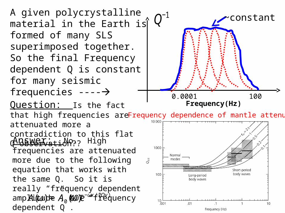
A given polycrystalline material in the Earth is formed of many SLS superimposed together. So the final Frequency dependent Q is constant for many seismic frequencies ----

100

€

Q−1

Frequency(Hz)

~constant

0.0001

Frequency dependence of mantle attenuationQuestion: Is the fact that high frequencies are attenuated more a contradiction to this flat Q observation??

Answer: No. High frequencies are attenuated more due to the following equation that works with the same Q. So it is really “frequency dependent amplitude”, NOT “frequency dependent Q”.

€

A(ω) ≈ A0(ω)e−ωx /(2Qv )

11

Eastern USA (EUS) and Basin-and-Range Attenuation

Mitchell 1995 (lower attenuation occurring at high frequencies, tells us that frequency independency is not always true

Low Q in the asthenosphere, Romanowicz, 1995

12

An example of Q extraction from differential waveforms.Two phases of interest:

sS-SsScS - ScS

Flanagan & Wiens (1990)

13

Key Realization: The two waveforms are similar in nature, mainly differing by the segment in the above source (the small depth phase segment)

€

sS(ω) ≈ S(ω)R(ω)A(ω)

€

sS(ω) = frequency spec of sS

S(ω) = frequency spec of S

R(ω) = crustal operator

A(ω) = attenuation operator of interest

Approach: Spectral division of S from SS, then divide out theCrustal operator (a function in freq that accounts for the of the additional propagation in a normal crust)

Spectral dividing S and R will leave the attenuation term A(w)

€

A(ω) = e−ωt / 2Q ⇒ log( A(ω) ) = −t

2Qω

(slope = =t/2Q, t = time diff of sS-S)